2006_marino.pdf-1dacd30a3dca10e1ed5f11778c25e905
TRANSCRIPT

Paints quantified
Image analytical studies of preparatory grounds used by Van Gogh
Beatrice Marino

The work described in this thesis was performed at AMOLF (FOM Institute of Atomic and Molecular Physics, Kruislaan 407, 1098 SJ Amsterdam, The Netherlands), and benefited greatly from the strong collaboration with the Conservation Department of the Van Gogh Museum. The research is part of the ‘De Mayerne’ programme funded by the Dutch Organization for Scientific Research (NWO) and supported by the Foundation for Fundamental Research on Matter (FOM), a subsidiary of the Dutch Organization for Scientific Research (NWO). This research is embedded in the FOM research program nr. 49 ‘Mass spectrometric imaging and structural analysis of biomacromolecules’. © Beatrice Marino ISBN-10: 90-77209-19-0 ISBN-13: 978-90-77209-19-6 Cover illustration by Beatrice Marino. The cover is a photographic mosaic made from ‘Self-portrait with felt hat’ (F296) by Vincent van Gogh (Van Gogh Museum, Vincent van Gogh Foundation, Amsterdam). The software used for creating the mosaic is AndreaMosaic by Andrea Wetzler, available at http://www.andreaplanet.com Can you find Wally in the cover?

Paints quantified
Image analytical studies of preparatory grounds used by Van Gogh
ACADEMISCH PROEFSCHRIFT
ter verkrijging van de graad van doctor aan de Universiteit van Amsterdam op gezag van de Rector Magnificus prof. mr. van der Heijden ten overstaan van een
door het college voor promoties ingestelde commissie, in het openbaar te verdedigen in de Aula der Universiteit
op woensdag 18 oktober 2006, te 12.00 uur
door
Beatrice Marino
geboren te Rome, Italië

Promotiecommissie Promotor: Prof. Dr. J.J. Boon Overige commissieleden: Prof. Dr. D. Frenkel
Prof. Dr. R.M.A. Heeren Prof. Dr. P.G. Kistemaker Prof. Dr. C.G. de Koster
Dr. J. Townsend Prof. Dr. Ir. L.J. van Vliet
Faculteit der Natuurwetenschappen, Wiskunde en Informatica

MOLART REPORTS This thesis is the twelfth in the series if MOLART reports. The MOLART reports summarise research results obtained in the course of the MOLART and De Mayerne Research Programmes supported by NWO (Dutch Organization for Scientific Research). Information about the MOLART reports can be obtained from Prof. Dr. J.J. Boon, FOM-Institute for Atomic and Molecular Physics, Kruislaan 407, 1098 SJ Amsterdam, The Netherlands. [email protected]. 1. Molecular studies of fresh and aged triterpenoid varnishes, Gisela A. van der
Doelen, 1999. ISBN 90-801704-3-7
2. A mathematical study on craquelure and other mechanical damage in
paintings, Petri de Willigen, 1999. ISBN 90-407-1946-2
3. Solvent extractable components of oil paint films, Kenneth R. Sutherland,
2001. ISBN 90-801704-4-5
4. Molecular changes in egg tempera paint dosimeters as tools to monitor the
museum environment, Oscar F. van den Brink, 2001. ISBN 90-801704-6-1
5. Discoloration in Renaissance and Baroque oil paintings, Margriet van Eikema
Hommes, 2004. Archetype Publications, London.
6. Analytical chemical studies on traditional linseed oil paints, Jorrit D.J. van
den Berg, 2002. ISBN 90-801704-7-X
7. Microspectroscopic analysis of traditional oil paint, Jaap van der Weerd, 2002.
ISBN 90-801704-8-8 8: Laser Desorption Mass Spectrometric Studies of Artists' Organic Pigments,
Nicolas Wyplosz, 2003. ISBN 90-77209-02-6

9. Molecular studies of Asphalt, Mummy and Kassel earth pigments: their characterisation, identification and effect on the drying of traditional oil paint, Georgiana M. Languri, 2004. ISBN 90-77209-07-7
10: Analysis of diterpenoid resins and polymers in paint media and varnishes;
with an attached atlas of mass spectra, Klaas Jan van den Berg (forthcoming). 11: Binding medium, pigments and metal soaps characterised and localised in
paint cross-sections, Katrien Keune, 2005. ISBN 90-77209-10-7
12: Paints quantified: image analytical studies of preparatory grounds used by
Van Gogh, Beatrice Marino, 2006. ISBN-10: 90-77209-19-0 ISBN-13: 978-90-77209-19-6
Published MOLART reports can be ordered from Archetype Publications, 6 Fitzroy Square, London W1T 5HJ, England, Tel: +44 207 380 0800 Fax: +44 207 380 0500, [email protected].

CHAPTER 1 INTRODUCTION 1 1.1 Van Gogh studies within the De Mayerne Programme 2 1.2 Commercial supports and the practice of Vincent van Gogh in the Paris period
3 1.3 Commercial preprimed supports manufacture in the 19th century 4 1.4 Case study of selected commercial ground paints in paintings by Vincent
van Gogh. Previous investigations 6 1.5 Qualitative versus quantitative analysis 9 1.6 Thesis structure 13 1.7 Acknowledgements 14 1.8 References 15 FIGURES OF CHAPTER 2 18 CHAPTER 2 IMAGING-SIMS CHARACTERIZATION OF SELECTED GROUND PAINTS IN PAINTINGS BY VAN GOGH 51 2.1 Introduction 52 2.2 Materials 53 2.2.1 Samples 53 2.2.2 Analytical techniques 53 2.3 Interpretation of SIMS data 55 2.3.1 Identification from SIMS data of paint materials 56 2.3.2 Identification by SIMS of materials in the ground paint 57 Lead white 57 Calcium carbonate and gypsum 57 Barium sulphate 58 Clay, alumina, and alum 58 Ultramarine 59 Earth pigments and carbon black 59

Magnesium-rich opaline silica (menilite) 59 2.3.3 Identification by SIMS of materials in the upper paint layer 60 Lead white 60 Zinc white 61 Prussian blue 61 Viridian 61 Cobalt blue and copper-based blue pigments 61 Vermilion 62 Earth pigments 62 2.3.4 Identification of the binding medium by SIMS 62 2.3.5 Analysis of paint texture in SIMS maps 63 2.4 Case study 64 2.4.1 Plaster figure of a female torso (F216a, mid. June 1886) 64 2.4.2 Plaster figure of a female torso (F216b, mid. June 1886) 67 2.4.3 Plaster figure of a female torso (F216d, mid. June 1886) 69 2.4.4 Plaster figure of a male torso (F216e, mid. June 1886) 71 2.4.5 Plaster figure of a kneeling musculature model (F216f, mid. June 1886)73 2.4.6 Plaster figure of a female torso (F216j, mid. June 1886) 75 2.4.7 Self-portrait with straw hat (F267, March-June 1887) 77 2.4.8 Portrait of Theo (F294, Summer 1887) 79 2.4.9 Self-portrait with felt hat (F296, Summer 1887) 81 2.4.10 Woman by a cradle, portrait of Leonie Rose Davy-Charbuy (F369, August-September 1887) 83 2.5 Technical discussion and conclusions 85 2.6 Acknowledgements 90 2.7 References 90 APPENDIX TO CHAPTER 2 93 A.2.1 Menilite, the Paris Basin, and paint manufacturing and trading 94 A.2.2 Chert and menilite 95 A.2.3 Geology of the Paris Basin 96 A.2.4 Observations on the characteristics of other materials found in paints 98 Calcium carbonate 98 Gypsum 99 Clays 99 Barite 99 A.2.5 Final comments 100 A.2.6 Acknowledgements 100 A.2.7 References 101

CHAPTER 3 QUANTITATIVE COLOUR ANALYSIS OF GROUND PAINTS IN PAINT CROSS-SECTIONS 103 3.1 Introduction 104 3.2 Materials 106 3.2.1 Samples 106 3.2.2 Acquisition of light-microscopic digital images 106 3.2.3 Data analysis 107 3.3 Method of colour comparison in digital images 107 3.3.1 Colour in digital images and histogram of an image 107 3.3.2 Measure of similarity by histogram quadratic distance 108 3.3.3 Classification by hierarchical clustering methods 109 3.4 Discussion of the case study: grounds in paintings by van Gogh 111 3.5 Conclusions 114 3.6 Acknowledgements 115 3.7 References 115 FIGURES OF CHAPTER 3 117 FIGURES OF CHAPTER 4 124 CHAPTER 4 QUANTITATIVE ANALYSIS OF COMPOSITION OF GROUND PAINTS IN PAINT CROSS-SECTIONS 141 4.1 Introduction 142 4.2 Materials 143 4.2.1 Samples and analytical techniques 143 4.2.2 Data processing 143 4.3 Methodology of comparison of the material composition 144 4.3.1 General concepts 144 4.3.1.1 Analogy between colour images and imaging mass-
spectrometric data 144 4.3.1.2 Adapting the method of colour comparison to imaging SIMS data 145 4.3.2 First step: data reduction and feature extraction 145 4.3.2.1 Importing datasets 146 4.3.2.2 Feature selection 147 4.3.2.3 Selection of regions of interest 147 4.3.2.4 Principal component analysis 148 PCA as a compression tool 148

Formulation of PCA 149 PCA as a tool for data comparison and classification 150 4.3.2.5 Reduction of number of intensity levels 150 4.3.2.6 Stacks and RGB composites of score images 151 4.3.3 Second step: histogram extraction 151 4.3.4 Third step: histogram comparison 152 4.3.5 Classification by hierarchical cluster analysis 152 4.4 Case study: grounds in paintings by van Gogh 153 4.4.1 Application to the datasets 153 4.4.2 Analysis of PCA output 154 4.4.2.1 Loadings and score images 155 4.4.2.2 RGB composites of score images 155 4.4.2.3 Choice of number of intensity levels 156 4.4.3 Correspondence between colours in RGB composites and sample
composition 156 4.4.4 Analysis of the cluster solution 157 4.4.4.1 Case of 3 colours per channel 157 4.4.4.2 Case of 9 colours per channel 158 4.4.4.3 Additional and final considerations 158 4.5 Conclusions 163 4.6 Acknowledgements 164 4.7 References 165 CHAPTER 5 QUANTITATIVE ANALYSIS OF TEXTURE OF GROUND PAINTS IN PAINT CROSS-SECTIONS 167 5.1 Introduction 168 5.2 Texture, structure, and morphology 169 5.2.1 Definitions 170 5.2.1.1 General definitions 170 5.2.1.2 Texture and structure in image analysis and computer vision 170 5.2.1.3 Definitions in sedimentary geology 171 5.2.1.4 Definitions in paint industry and art conservation 172 5.3 Materials and methods 172 5.3.1 Samples and analytical techniques 172 5.3.2 Data processing 173 5.4 Method of texture analysis 174 5.4.1 Image processing and analysis 174 5.4.2 Image preprocessing 174

5.4.2.1 Smoothing filters 175 5.4.2.2 Bilateral filtering 175 5.4.3 Mathematical morphology 177 5.4.3.1 Area opening 177 Pixel connectivity 178 Connected component labelling 179 Terminology 179 5.4.3.2 Application of area opening to grey-scale Images 180 First step: Decomposing the image in level set images 181
Second step: Connected component labelling of level set images 182 Third step, segmentation result: Combining labelled level set images into a single image 183
Fourth step: Extraction of size distribution 184 5.5 Case study: selected grounds of van Gogh 184 5.5.1 SIMS general discussion 184 5.5.2 Comparison with SEM-EDX 187 5.5.3 Discussion of the case study 188 5.5.3.1 General comments 189 5.5.3.2 Discussion of individual samples 190 F216a/1 190 F216b/1 190 F216d/1 190 F216e/1 191 F216f/2 191 F216j/1 191 F267/2 191 F294/1 192 F296/2 192 F369/1 192 5.5.3.3 Summary 193 Lead white 193 Calcium 193 Barium sulphate 193 5.6 Conclusions 195 5.7 Acknowledgements 198 5.8 References 198

CHAPTER 6 A NANOSIMS STUDY OF A PAINT CROSS-SECTION FROM A GROUND OF VAN GOGH’S PLASTER FIGURE OF A FEMALE TORSO (f216J) 203 6.1 Introduction 204 6.2 Materials 205 6.2.1 Sample 205 6.2.2 Analytical techniques 205 6.3 Results 206 6.4 Conclusions 208 6.5 Acknowledgements 209 6.6 References 209 FIGURES OF CHAPTER 5 211 FIGURES OF CHAPTER 6 229 APPENDIX A 233 APPENDIX B 237 APPENDIX C 245 SUMMARY 259 SAMENVATTING 267 SOMMARIO 275 ACKNOWLEDGEMENTS-DANKWOORD-RINGRAZIAMENTI 283


Introduction
So, so you think you can tell Heaven from Hell,
Blue skies from pain. Can you tell a green field
from a cold steel rail? A smile from a veil?
Do you think you can tell?
Pink Floyd, ‘Wish you were here’
‘...where the “means-whereby” are right for the purpose, desired ends will come.’
F.M. Alexander, ‘The universal constant in living’

INTRODUCTION
2
1.1 VAN GOGH STUDIES WITHIN THE DE MAYERNE
PROGRAMME The work presented in this thesis is part of the Van Gogh project of the De Mayerne Programme, which aims at investigating different aspects of the artist’s working method in relation to contemporary practice, by following an interdisciplinary approach [Hendriks et al. 2006]. The project included documentary source research in Paris for information relating to the manufacture and retail of artist materials in late 19th century France. With a focus on Van Gogh’s suppliers, to assist in the reconstruction of the artist’s working practice. The HART project focused on making accurate reconstructions of a selection of Van Gogh’s prepared picture supports and paints, in order to get insight into the working properties and visual consequences of using these materials [Carlyle et al. 2005]. In this thesis an in-depth imaging analytical study of grounds in a group of pictures painted on ready-primed carton supports is conducted, to investigate the differences between the paints. The study follows a new approach based on quantitative analytical techniques. The broader aim is to develop new, quantitative techniques for comparing and classifying paint sample cross-sections.

INTRODUCTION
3
1.2 COMMERCIAL SUPPORTS AND THE PRACTICE OF VINCENT VAN GOGH IN THE PARIS PERIOD
The comparison and distinction between different formulations and different production batches of artist materials (supports, grounds, and paints) is useful for conservators and art historians. For example, technical studies have demonstrated that comparative investigation of self-made or ready-made picture supports of Van Gogh can help to establish a chronology for these pictures [Hoermann Lister et al. 2001, Hendriks 2006 and 2007], or even prove authenticity [Hendriks and van Tilborgh 2001]. The characterization of artist materials is also a useful aid for the understanding of the role and the influence of these materials in the stylistic evolutionary process of an artist. In recent papers, Hendriks and Geldof [2005] and Hendriks [2006 and 2007] discuss the types of prepared supports used by Van Gogh, how the type of support influenced his painting style and technique, and how they fit in the evolution of Van Gogh as a painter through his career. The reconstruction of the oeuvre of Vincent van Gogh in the Paris period is particularly problematic for art historians. In fact, stimulated by the extremely dynamic artistic environment of Paris, Vincent experienced a period of intnse technical and artistic experimentation, producing works that varied widely in style and technique within a time span of only two years. Unfortunately, since he lived in Paris with his brother Theo (with whom he used to exchange letters in other periods that are usually a rich source of information), there are virtually no letters to inform us on his creative goals, working procedures, and materials used in this period. Given this context, other sources of information on the materials and techniques employed by the painter are particularly valuable to help resolve open questions on issues of attribution and chronology. Like other painters of his day, in Paris Van Gogh made use of commercially prepared artist materials. Ready prepared artist’s materials started to become available to painters and artists late in the 19th century. Colourmen offered a wide range of different products and materials too meet the artist’s needs, including paint tubes, pre-primed canvases and cardboards, stretchers, and even ready-stretched primed canvases [Bomford et al. 1991, Callen 2000, Carlyle 2001, Constantin 2001, Roth-Meyer 2004]. Van Gogh used off-the-shelf painting supports first in Antwerp, where he enrolled at the Academy in November 1885, and then in Paris where he stayed in 1886-1888. At the time the trade of colour merchants selling artist materials flourished in Paris and especially in the artists quarters of Montmartre, Van Gogh visited several shops,

INTRODUCTION
4
as we know from retail stamps left on the back of his Paris works [Hendriks and Geldof 2005, Hendriks 2006 and 2007]. Even if not listed as manufacturers, many of these retailers were equipped to produce paints and supports by themselves, though presumably in small supplies. He purchased commercial canvases, in different sizes, fabrics and with grounds of varying compositions, tints, and absorbing properties. Van Gogh painted mostly on canvas, but already during his first weeks in Paris he used ready-primed cardboard supports (carton in French sources). Cartons were a cheaper alternative to canvases, and suitable for learning purposes. In this period he used cartons for a series of studies of plaster cast models and for self-portraits, some of which are the subject of the investigations presented in this thesis. All of the colourmen visited by Van Gogh are known to have supplied other Impressionists and Post-impressionists painters as well. The study of his painting materials is therefore relevant also to answer questions about his contemporaries, who very probably have used some of the very same materials. 1.3 COMMERCIAL PREPRIMED SUPPORTS MANUFACTURE
IN THE 19TH CENTURY A variety of modern and historical sources provide detailed information on the function of the ground, its composition, and preparation in the 19th century [Bomford et al. 1991, Callen 2000, Carlyle 2001]. The main function of the ground, which can be applied in one or multiple layers, is to prepare the painting support – either canvas, cardboard, or paper – to receive the paint layers. The ground paint has also an aesthetical role, as its colour, texture and absorbing properties affect the final appearance of the painting. The colour of the ground was especially important for the Impressionist and post-Impressionist painters, including Vincent van Gogh, who often used the ground as part of the finished composition or exposed between paint brushstrokes to achieve pictorial effects [Hendriks and Geldof 2005]. Supports were manufactured in a large variety of standard sizes, with canvases of different fabrics in various types of weaves. The preparatory layers were made in different tints and with different surface finishes and absorbing properties, and were realized through an endless variety of different paint formulations, containing any number of a whole range of available pigments, binders, driers, stabilisers and extenders. Supports might also be custom prepared by the colourmen on request from the artist. Alternatively, the artists could buy prepared canvas by the roll,
INTRODUCTION
5
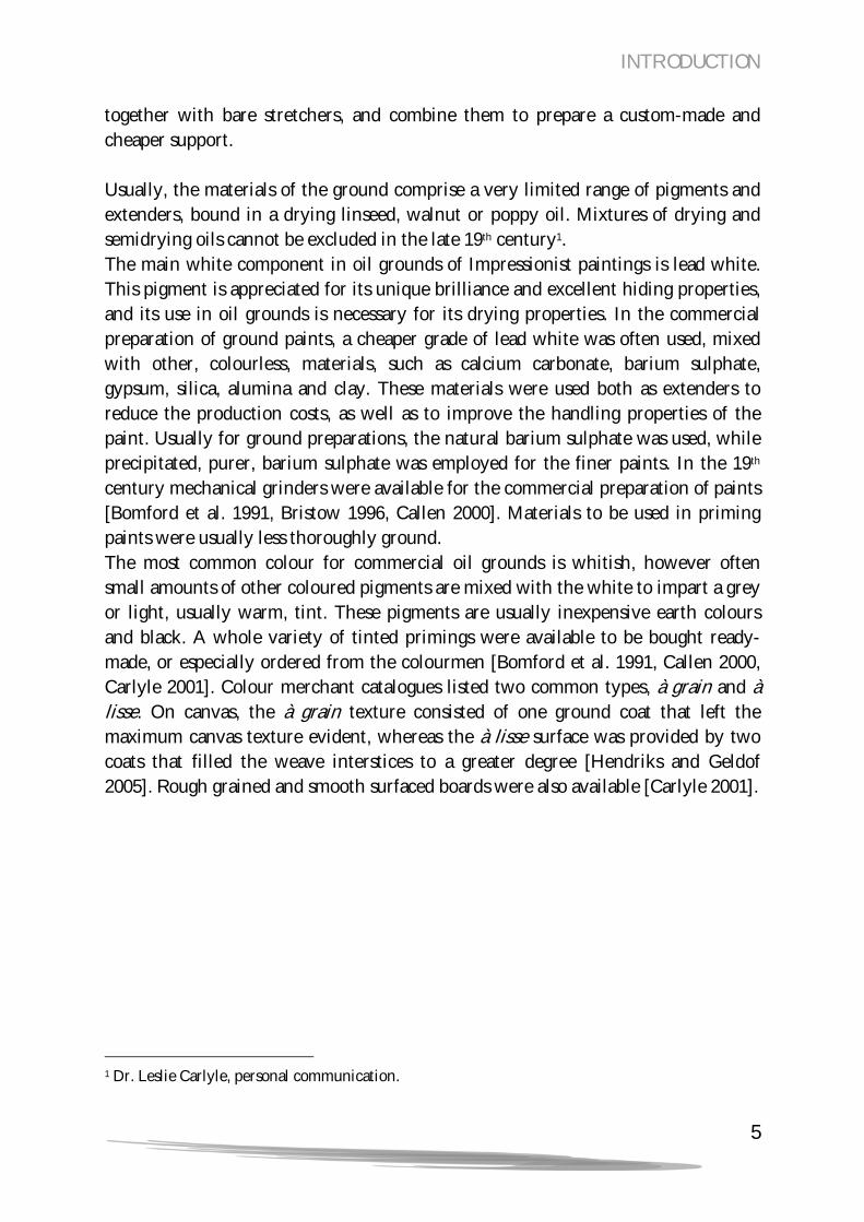
together with bare stretchers, and combine them to prepare a custom-made and cheaper support. Usually, the materials of the ground comprise a very limited range of pigments and extenders, bound in a drying linseed, walnut or poppy oil. Mixtures of drying and semidrying oils cannot be excluded in the late 19th century1. The main white component in oil grounds of Impressionist paintings is lead white. This pigment is appreciated for its unique brilliance and excellent hiding properties, and its use in oil grounds is necessary for its drying properties. In the commercial preparation of ground paints, a cheaper grade of lead white was often used, mixed with other, colourless, materials, such as calcium carbonate, barium sulphate, gypsum, silica, alumina and clay. These materials were used both as extenders to reduce the production costs, as well as to improve the handling properties of the paint. Usually for ground preparations, the natural barium sulphate was used, while precipitated, purer, barium sulphate was employed for the finer paints. In the 19th century mechanical grinders were available for the commercial preparation of paints [Bomford et al. 1991, Bristow 1996, Callen 2000]. Materials to be used in priming paints were usually less thoroughly ground. The most common colour for commercial oil grounds is whitish, however often small amounts of other coloured pigments are mixed with the white to impart a grey or light, usually warm, tint. These pigments are usually inexpensive earth colours and black. A whole variety of tinted primings were available to be bought ready-made, or especially ordered from the colourmen [Bomford et al. 1991, Callen 2000, Carlyle 2001]. Colour merchant catalogues listed two common types, à grain and à lisse. On canvas, the à grain texture consisted of one ground coat that left the maximum canvas texture evident, whereas the à lisse surface was provided by two coats that filled the weave interstices to a greater degree [Hendriks and Geldof 2005]. Rough grained and smooth surfaced boards were also available [Carlyle 2001].
1 Dr. Leslie Carlyle, personal communication.

INTRODUCTION
6
1.4 CASE STUDY OF SELECTED COMMERCIAL GROUND PAINTS IN PAINTINGS BY VINCENT VAN GOGH - PREVIOUS INVESTIGATIONS
The work described in the present thesis takes as starting point and source of information an earlier comparative study made by Hendriks and Geldof [2005], and worked out further in Hendriks [2006 and 2007], in which a detailed examination and analysis of the picture supports of 93 paintings by Van Gogh of the Antwerp and Paris period was performed. In this work the role, the evolution and the influence of the painting support in the development process of Van Gogh’s painting style and technique were addressed. In the present work, the choice is restricted to nine paintings of the Paris period that were examined earlier by Hendriks and Geldof, to investigate the grounds present on ready-primed cardboard or carton. Below we briefly summarize the approach, the method, and the results of this earlier comparative study (see also Table 1). Six of the paintings represent plaster cast model statuettes against a blue background (F216a, F216b, F216d, F216e, F216f, F216j), dated to mid. June 1886, two self-portraits (F267, F296) and one portrait of Theo van Gogh (F294), dated to 1887. These paintings were painted on ready-prepared cartons with commercial grounds. A random control sample of ground from a 1887 woman’s portrait made on canvas was included (F369)2 Illustrations of the paintings can be found in Appendix A at the end of this Thesis. The study was performed on the basis of traditional investigational criteria, obtained from visual and technical examinations made on various characteristics of the supports. These include colour and texture of the surface of the ground layer, features of the cardboard support, and build-up and composition of the ground paint. All the boards show identical features of construction, in terms of their consistent 2 mm thickness, build-up in two layers of hard-pressed and poorly refined wood pulp. The supports have four different formats. The priming layers were prepared in white (F216a, F216b), pale grey (F216d, F216e, F216f, F216j, F267, F294, F296), and whitish (F369). The grounds on carton have been worked to provide a smooth surface texture. Superficial tooling marks in the surfaces of the grounds suggested
2 The F-numbers of the paintings refer to their identifying numbers in the oeuvre catalogue of De la Faille [1970].

INTRODUCTION
7
that these were first brushed on, then smoothed by light sanding or scraping that left fine parallel scratches. The ground surface of painting F369 was not rolled on or brushed; the canvas texture plays through to a greater extent than for smooth cartons, but the application of the ground paint in two layers produces a relatively smooth surface. Stereo-microscopic examination made on the edges of the primed cardboard supports has shown that the standard sized supports were cut from larger pre-primed sheets, most likely manufactured in the Paris region where factories producing cartons were known in the period. Three supports (F267, F294, and F296) retain their original edges intact, providing physical evidence that the ground was sliced through sharply when the supports were cut to size, and overlying brush strokes run over the support edges [Hendriks and Geldof 2005]. SEM-EDX analysis was performed on samples of the preparatory ground layers. Paint cross-sections were made from samples taken from the edges of the paintings and embedded in Polypol (polyester). All samples include the ground layer; in some cases a paint layer and/or part of the support are also present. The analysis revealed two standard recipes of mixed paint used for pale grey and white types of grounds on cardboard, all applied in a single layer. The white grounds contained lead white, calcium carbonate, and traces of fine black. The pale grey grounds contained lead white, a little barium sulphate, gypsum, black and a few particles of different shades of ochre pigment. The control whitish ground on canvas has been applied in two stages and consists of a white layer on top of a beige layer. Both layers contain lead white, gypsum and barium sulphate, and ochres, the latter with less ochre present in the top white layer. Original trade stickers surviving on the back of several plaster cast model cartons inform us that they were purchased from the shop of Pignel-Dupont, established at number 17 rue Lepic, just down the street from the brother’s apartment where Vincent moved in June 1886, when the works are thought to have been painted. In the case of F216a, F216b, F216e, F216f, and F216j the stickers were transferred from the backs of the cartons to backing supports applied in 1929. No stickers were evident on the back of F216d, though these might be hidden by the marouflage backing, or have been irrevocably damaged during attempted transfer. The three tiny portraits, which do not bear labels from the shop of Pignel-Dupont, are dated to 1887 on the basis of style, as is the woman’s portrait on canvas (F369). The results of the investigation point to a distinction in a group of white grounds and a second group of grey grounds, the latter subdivided into two smaller subgroups, possibly from two different batches (see Table 1).

8
INTRODUCTION
Tabl
e 1.
Lis
t of
pai
ntin
gs u
nder
stu
dy w
ith
info
rmat
ion
on t
he p
rim
ed s
uppo
rts
on c
arto
n. P
aint
ing
F36
9 (r
ando
m c
ontr
ol s
ampl
e)
is m
ade
on c
anva
s. Th
e ab
brev
iati
ons
for
the
mat
eria
ls l
iste
d un
der
the
com
posi
tion
are
: L
W =
lea
d w
hite
, CC
= ca
lciu
m
carb
onat
e, B
= b
arit
e, G
= g
ypsu
m, C
B =
car
bon
blac
k, B
B =
bon
e bl
ack,
EP
= e
arth
pig
men
t.
Pa
intin
g F-
num
ber
Title
Co
lour
of g
roun
d pa
int s
urfa
ce
Com
posit
ion
of g
roun
d pa
int
(SEM
-ED
X, m
icro
chem
ical
anal
ysis)
Form
at a
nd si
ze
of th
e su
ppor
t H
ypot
hetic
al
clas
sific
atio
n
F2
16a
Plas
ter f
igur
e of
a fe
mal
e to
rso
Whi
te
LW, C
C 8
(46
cm x
38
cm)
1
F2
16b
Plas
ter f
igur
e of
a fe
mal
e to
rso
Whi
te
LW, C
C 8
(46
cm x
38
cm)
1
F2
16d
Plas
ter f
igur
e of
a fe
mal
e to
rso
Pal
e gr
ey
LW,
B (li
ttle)
, G
, bl
ack,
EP
(few
pa
rtic
les)
5
(35
cm x
27
cm)
2a
F2
16e
Plas
ter f
igur
e of
a m
ale
tors
o P
ale
grey
LW
, B (l
ittle
), G
, CB,
CC
5 (3
5 cm
x 2
7 cm
) 2a
F2
16f
Plas
ter f
igur
e of
a k
neel
ing
mus
cula
r mod
el
Pal
e gr
ey
LW,
B (li
ttle)
, G
, CB
, EP
(fe
w
part
icle
s)
5 (3
5 cm
x 2
7 cm
) 2a
F2
16j
Plas
ter f
igur
e of
a fe
mal
e to
rso
Pal
e gr
ey
LW,
B (li
ttle)
, G
, CB
, EP
(fe
w
part
icle
s)
5 (3
5 cm
x 2
7 cm
) 2a
F2
67
Self-
port
rait
with
stra
w h
at
Pal
e gr
ey
LW,
B (li
ttle)
, G
, CB
, EP
(fe
w
part
icle
s)
0 (1
9 cm
x 1
4 cm
) 2b
F2
94
Port
rait
of T
heo
Pal
e gr
ey
LW,
B (li
ttle)
, G
, CB
, EP
(fe
w
part
icle
s)
0 (1
9 cm
x 1
4 cm
) 2b
F2
96
Self-
port
rait
with
felt
hat
Pal
e gr
ey
LW,
B (li
ttle)
, G
, CB
, EP
(fe
w
part
icle
s)
0 (1
9 cm
x 1
4 cm
) 2b
F3
69
Wom
an b
y a
crad
le,
port
rait
of L
eoni
e Ro
se
Dav
y-Ch
arbu
y W
hitis
h W
hite
gro
und:
LW
, bla
ck p
artic
les
Beig
e gr
ound
: LW
, BB,
EP
6 (4
1 cm
x 3
3 cm
) ex
tra

INTRODUCTION
9
1.5 QUALITATIVE VERSUS QUANTITATIVE ANALYSIS Features that are traditionally used for the characterization and comparative studies of paints include colour, composition, and texture. The colour of each paint layer, including that of the ground paint, has an impact on the final appearance of a picture. In fact, the colour visible on the paint surface is the result of a series of interactions of light inside the paint layers, and is dependent on optical, compositional, structural and geometrical properties of the paint materials [Völz 2001]. The size of particles of the paint materials also influences consistency, workability and handling properties of paint [Carlyle et al. 2005, Patton 1979]. For example, differences in size distributions result in different volume degrees of pore space that can be filled by the binding medium, producing paints of different rheological properties and thus workability [Patton 1979, Stoye 2001]. Significant variations in particle size distribution and morphology can be observed even for the same material, depending on manufacturing and grinding method. Figures 1 and 2 show a few examples for lead white paints in oil in ground paint reconstructions [Carlyle et al. 2005] and in grounds in paintings by Van Gogh. Colourless extenders of certain coarseness may be added to adjust the paint consistency. This micro-structure within the paint layer, which we define as compound texture and that will be the focus of part of this Thesis, is related to the surface texture or feeling of the painted surface3. The coarseness and the surface texture of a paint layer affect the application of upper paint layers and the final visual appearance of the painting, and contribute to the creation of surface textural effects. It is evident that colour, composition, and texture are interrelated in a complex way. However, often information on these properties is used only qualitatively, for example to identify the materials in the paint by examining only a few particles in paint cross-sections. Colour and texture of the paint surface are also often characterized in descriptive terms. The traditional approach used for the analysis and comparison of paintings and artist materials, although effective in many studies, has several shortcomings. For example, it is often hard to make a valid assessment of the colour of a paint or ground paint, which may be largely masked by paint layers on top, or distorted by accumulated grime and restoration materials. The impression of the colour is subjective to viewing conditions that include light and other colours on the painting surface. In addition, the same colour can be achieved with paint formulations that differ in the type and individual colour of the materials used. For a painter the
3 The definitions of surface texture and compound texture will be given and discussed in Chapter 5. Compound texture will also be considered in descriptive terms in Chapter 2.

INTRODUCTION
10
Figure 1. BSE images of lead white ground paint reconstructions (HART project), prepared with different grinding processing methods, show large differences in particle size. The reconstructions were made with lead white, produced according to the Dutch ‘stack’ process, washed (a, b), and unwashed (c). Paints were prepared by mixing the pigment in washed linseed oil with a palette knife (a), ground fully on a
glass slab with a glass muller (b), and ground with a three-roller mill (c). Pictures by courtesy of Dr. Leslie Carlyle. colour of the ground is a decisive factor irrespective of how this colour has been achieved by the colourman preparing the preprimed canvas. For example, on the microscopic scale relatively few dark particles in a light matrix or a layer that is uniformly tinted may produce the same surface colour at the macroscopic level. Equally, comparison of ground samples may prove inconclusive, since it is uncertain whether slight variations either in colour, composition, or texture, simply reflect the inhomogeneous character of hand-mixed paints, or real differences in paint formulation. The complexity is further increased when a wide variety of possible ingredients must be taken into account. Another disadvantage of the subjective character of qualitative investigations is that often attention is paid to few specific features that are striking to the eye but that are not fully representative for the object being analysed. Also, the complexity of the character of certain features makes it difficult to formulate an appropriate and accurate description. For example, texture has a number of perceived qualities that depend on the viewing conditions, such as scale, contrast, orientation and shape of elements or objects that constitute the structure. In general, variations in object characteristics form a continuum with

INTRODUCTION
11
Figure 2. Examples of BSE images showing differences in particle size for lead white (in white) in ground paints in paintings by Vincent van Gogh. Samples: F293/8 (a, b), F216b/1 (c), F216d/1.

INTRODUCTION
12
no sharp limits that clearly define distinct classes. In addition, different characteristics, for example colour, composition, and texture are not independent but are correlated in a complex way. The difficulties increase considerably when the comparison is made between materials that exhibit strong similarities, so that a qualitative description becomes insufficient to characterize the differences. These considerations strongly indicate the need for a different analytical approach to complement the traditional qualitative characterization. Such an approach should have a quantitative character to provide full characterizations of the attributes of the objects under study. Qualitative analysis helps to identify the attributes that are potentially relevant for the specific study, to formulate hypotheses, and to design the aspects of further, quantitative investigations. Quantitative analysis provides a deeper insight on specific attributes through objective, accurate and statistically representative characterizations of the measured properties, can highlight features that were overlooked in the qualitative observations, and is able to test hypotheses. In a comparative type of study the quantitative character of the analysis provides a means of measuring the degree of difference or similarity between objects. The combined findings of qualitative and quantitative research deliver a comprehensive characterization of the subject matter. The work described in this thesis explores a new, quantitative approach in comparative studies of paint cross-section. The approach is to develop an analytical method, by choosing and combining statistical and image analytical tools, in order to obtain a description that represents efficiently the main characteristics and hence the differences between the ground paints. The specific aim is to chart differences within this group of ready-manufactured supports, prepared with standard ground recipes, in terms of differences in colour, composition, and particle size distribution of materials, and of the type of binding medium employed. A combination of light-microscopy, SIMS, SEM-EDX, and GC-MS should offer a more comprehensive and exact fingerprint of the materials present in cross-sections. The imaging data obtained by light microscopy and SIMS will be analysed and quantified using statistical multivariate and image analysis techniques.

INTRODUCTION
13
1.6 THESIS STRUCTURE In Chapter 2 we first discuss the data obtained by imaging SIMS on the paint cross-sections under study. SIMS data shows that there are clear differences in composition and compound texture between the ground paints. Characteristic elements of the ground paints are identified, and the corresponding SIMS maps discussed in this chapter will be used in Chapters 4 and 5 to make a quantitative comparison of the ground paints on the basis of composition and texture. Binding medium characterization is performed by SIMS and GC-MS. Complementary SEM-BSE and -EDX analysis is performed to answer specific compositional questions. In Chapters 3, 4, and 5 quantitative comparison of the ground paints is performed on the basis of different characteristics, measured at the microscopic level. Image processing and pattern recognition techniques are employed to enhance and extract this information from the samples. The features considered are the colour content of light microscopic images of samples (Chapter 3), the material composition of the ground paints derived from SIMS data (Chapter 4), and the texture of the paint characterized by particle size distributions in SIMS images (Chapter 5). In Chapter 3 we compare the ground paints on the basis of their colour as seen in light-microscopic images of the paint cross-sections. Colour histograms are used to represent the colour information of the ground paints. The similarity between the colours of the paints is measured by calculating a weighted distance between the histograms, and the classification is obtained with hierarchical clustering techniques. In Chapter 4 we adapt the methodology used in Chapter 3 for application to imaging SIMS data, as a means to compare composition information. Data reduction and feature extraction are essential steps to reduce data complexity and computational effort, to extract relevant discriminating features, and to improve the quality of the classification. Characteristic elements identified in Chapter 2 are hand selected, and Principal Component Analysis is used for further data reduction. The resulting imaging data sets are then processed in the same fashion as the colour images in Chapter 3. In Chapter 5 we quantify the compound texture of the main ground paint components from SIMS maps of characteristic elements identified in Chapter 2. The method presented here is based on bilateral filtering for noise suppression and

INTRODUCTION
14
mathematical morphology to identify and measure the size of particles in SIMS images. The advantage of working on SIMS images rests in the partial separation of particles into different chemical phases. This simultaneously simplifies the task of particle segmentation, and allows measuring the size distribution of particles from different materials. In Chapter 6 we explore the potential of a new generation of ion microprobes, NanoSIMS, for the analysis of paint cross-sections. The higher spatial and mass resolution, the higher secondary ion collection efficiency, and the capability of precise isotopic characterization could provide additional information not obtainable by SIMS. In particular, we give special attention to the distribution of characteristic elements, to finer structural and sub-structural details, and to isotopic ratio characterization of barite particles in the ground paint. 1.7 ACKNOWLEDGEMENTS Samples were provided by Ella Hendriks of the Van Gogh museum of Amsterdam. Initial preparation and light microscopy of paint samples was performed by Muriel Geldof at the Netherlands Institute for Cultural Heritage, in collaboration with Kees Mensch at the Shell Research and Technology Centre in Amsterdam for SEM-EDX analysis. We thank Dr. Leslie Carlyle of the Tate Gallery of London for kindly providing the images of lead white ground paint reconstructions of the HART project.

INTRODUCTION
15
1.8 REFERENCES DE LA FAILLE, J.-B., 1970 (1st ed. 1928). The works of Vincent van Gogh; his paintings and drawings, Reynal and Company, Amsterdam. BOMFORD, D., Kirby, J., Leighton, J., and Roy, A., 1991. Art in the making: Impressionism, National Gallery London Publications, Yale University Press, New Haven and London. BRISTOW, I.C., 1996. Interior house-painting colours and technology 1615-1840, Yale University Press, New Haven and London. CALLEN, A., 2000. The art of Impressionism: painting technique & the making of modernity, Yale University Press, New Haven and London. CARLYLE, L., 2001. The artist’s assistant: oil painting instruction manuals and handbooks in Britain 1800-1900 with reference to selected eighteenth century sources, Archetype Publications, London. CARLYLE, L., Witlox, M. et al., 2005. HART project report. Report of the De Mayerne Programme project: Historically Accurate Reconstructions of Oil Paint and Painting Composites. CONSTANTIN, S., 2001. The Barbizon painters: a guide to their suppliers, Studies in Conservation, 46, p. 49-67. HENDRIKS, E. 2006. Van Gogh’s working practice; a technical study, and Developing technique and style, essays in: Hendriks, E., and van Tilborgh, L., In relation to Van Gogh; a technical and art historical study of his Antwerp and Paris paintings in the Van Gogh Museum, PhD dissertation, Faculty of Humanities, University of Amsterdam (to be defended on 15th November 2006). HENDRIKS, E. 2007. Van Gogh’s working practice; a technical study, and Developing technique and style, essays in: van Tilborgh, L., and Hendriks, E., Vincent van Gogh paintings, Antwerp and Paris 1885-1888, volume 2, Van Gogh Museum, Amsterdam and Zwolle. HENDRIKS, E., Constantin, S., and Marino, B., 2006. Various approaches to Van Gogh technical studies: common grounds?, De Mayerne Highlights 2006.

INTRODUCTION
16
HENDRIKS, E., and Geldof, M., 2005. Van Gogh’s Antwerp and Paris picture supports (1885-1888) reconstructing choices, ArtMatters Netherlands Technical Studies in Art, 2, p. 39-74. HENDRIKS, E., and van Tilborgh, L., 2001. Van Gogh’s ‘Garden of the asylum’: genuine or fake?, The Burlington Magazine, p. 145-155. HOERMANN LISTER, K., Peres, C. and Fiedler, I., 2001. Tracing an interaction; supporting evidence, experimental grounds. In D. Druick and P. Kort Zegers, Van Gogh and Gauguin; The Studio of the South, The Art Institute of Chicago, p. 364-366. PATTON, T.C., 1979. Paint flow and pigment dispersion, John Wiley and Sons, New York. ROTH-MEYER, C., 2004. Les marchands de couleurs à Paris au dix-neuvième siècle, Doctoral thesis, Université Paris IV Sorbonne. VÖLZ, H.G., 2001. Industrial color testing: fundamentals and techniques, 2nd ed., Wiley-VHC.


FIGURES of CHAPTER 2
18
Figure 1. Examples of SIMS spectra in positive (a, c) and negative (b, d) ion mode of the paint cross-sections under investigation (X = poly(dimethyl siloxane), poly(ester), and phtalate contaminations; the peak at m/z 115 is produced by indium ions used to probe the sample surfaces).

FIGURES of CHAPTER 2
19
Figure 2. Example of identification by SIMS of lead white from the map of lead. Chloride is also introduced in the manufacturing process. An overlay of lead and chloride SIMS maps (a) and a line scan though the paint cross-section (b) show correlation between their intensity distributions. The arrow indicates the direction of the line scan. (Sample: F216j/1).
FIGURES of CHAPTER 2
20
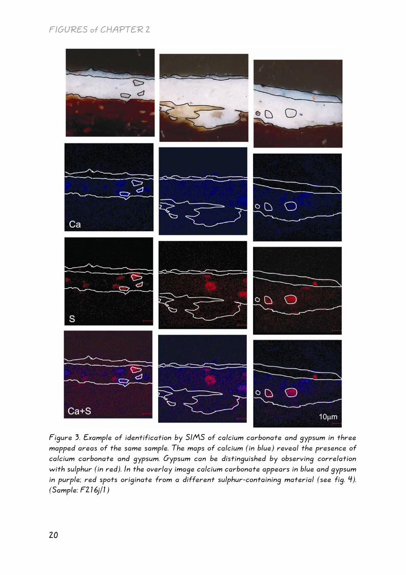
Figure 3. Example of identification by SIMS of calcium carbonate and gypsum in three mapped areas of the same sample. The maps of calcium (in blue) reveal the presence of calcium carbonate and gypsum. Gypsum can be distinguished by observing correlation with sulphur (in red). In the overlay image calcium carbonate appears in blue and gypsum in purple; red spots originate from a different sulphur-containing material (see fig. 4). (Sample: F216j/1)

FIGURES of CHAPTER 2
21
Figure 4. Example of identification by SIMS of barium sulphate from the maps of barium and sulphur. (a) Sulphur spots that in Figure 3 were not originating from gypsum may for instance be produced by barium sulphate. In the overlay image of individual maps of calcium (blue), barium (red), and sulphur (green), gypsum appears in greenish-blue and barium sulphate in yellow. (b) Traces of strontium are indicative of natural barium sulphate. The overlay image of barium (blue) and strontium (red) shows in purple co-occurrence of these two elements in the mineral particles. (Sample: F216j/1)
Figure 5. Example of appearance under SIMS of some aluminium-containing materials. Aluminium (in blue) is indicative of aluminium oxide, and, with potassium (in red), of clay and alumina (in purple in the overlay image). Aluminium oxide is used as a paint extender and a support for lakes; alumina may be present from the manufacturing process of lakes. (Sample: F216j/1)

FIGURES of CHAPTER 2
22
Figure 6 (above). Example of identification by SIMS of ultramarine. Co-occurrence of aluminium (in blue) and sodium (in red) in blue pigment particles (see light-microscopic image on right side) reveals presence of ultramarine (purple in the overlay image).
Figure 7 (left). Example of identification by SIMS of earth pigments from the map of iron. (Sample: F216j/1)
Figure 8 (below). The magnesium-rich variety of chert appears in SIMS in the maps of magnesium and silicon (a). Silicon carbide produces mass peaks that overlap with magnesium and silicon, and particles of chert can be distinguished with SEM-EDX (b).
BSE images of the same particles showing the laminated structure at the micron scale (c). (Sample: F216a/1)

FIGURES of CHAPTER 2
23
Figure 9. Example of identification by SIMS of zinc white from the map of zinc. (Sample: F216a/1)
Figure 10. Examples of identification by SIMS of some blue and green pigments in the upper blue paint layer in one of the samples under investigation. The Figure shows viridian in the chromium map (a), a blue copper-based pigment in the copper map (b), cobalt blue in the maps of cobalt and aluminium (c). (Sample: F296/2)

FIGURES of CHAPTER 2
24
Figure 11. Detail of the SIMS chromium map of Figure 10 around a viridian particle in sample F296/2 (left), compared with the BSE image of the same area (right). The chromium map clearly reflects the particle morphology that is visible in the BSE image.
Figure 12. Example of identification by SIMS of vermilion from the map of sulphur (a). Since mercury is not detected by SIMS, comparison with a light-microscopic image (b) of the mapped area is necessary. Additional evidence can be obtained by electron microscopy in a BSE image (c) where vermilion appears of light grey. (Sample: F216a/1)
Figure 13. Example of earth pigment in the upper blue paint seen by SIMS. (Sample: F216a/1)
Figure 14. Examples of SIMS distribution maps of the characteristic peaks of the binding medium palmitic fatty acid (FA C16) and stearic fatty acid (FA C18). (Sample: F216a/1)

FIGURES of CHAPTER 2
25
Figure 15. Paint cross-section F216a/1, light-microscopic images under visible (top) and UV light (bottom). The rectangular outlines in the light-microscopic images (A, B, C) indicate the areas mapped with SIMS.
Figure 16. Paint cross-section F216a/1, SIMS total ion current image and distribution maps of characteristic elements in positive mode.

FIGURES of CHAPTER 2
26
Figure 17. Paint cross-section F216a/1, SIMS distribution maps of characteristic elements in positive mode.

FIGURES of CHAPTER 2
27
Figure 18. Paint cross-section F216a/1, SIMS total ion current image and distribution maps of characteristic elements in negative mode.

FIGURES of CHAPTER 2
28
Figure 19. Paint cross-section F216b/1, light-microscopic images under visible (top) and UV light (bottom). The rectangular outlines in the light-microscopic images (A, B, C, D) indicate the areas mapped with SIMS.

FIGURES of CHAPTER 2
29
Figure 20. Paint cross-section F216b/1, SIMS total ion current image and distribution maps of characteristic elements in positive mode.

FIGURES of CHAPTER 2
30
Figure 21. Paint cross-section F216b/1, SIMS total ion current image and distribution maps of characteristic elements in negative mode.

FIGURES of CHAPTER 2
31
Figure 22. Paint cross-section F216d/1, light-microscopic images under visible (top) and UV light (bottom). The rectangular outlines in the light-microscopic images (A, B) indicate the areas mapped with SIMS.
Figure 23. Paint cross-section F216d/1, SIMS total ion current image and distribution maps of characteristic elements in positive mode.
FIGURES of CHAPTER 2
32
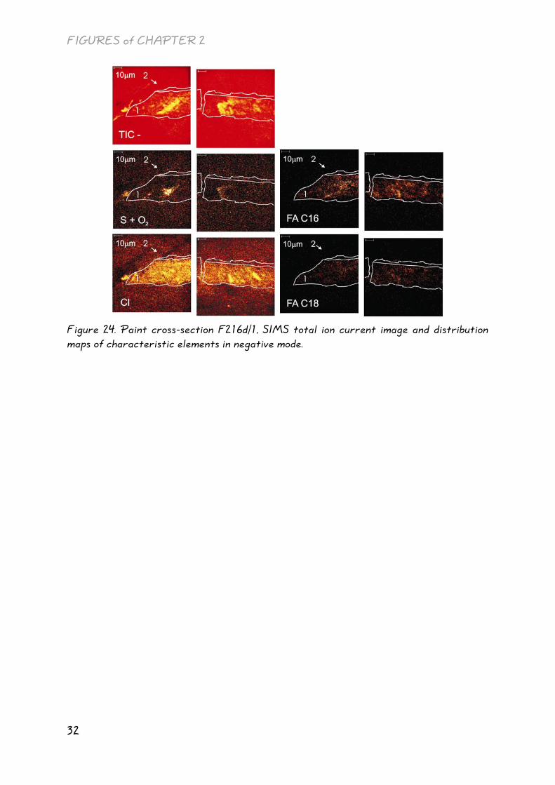
Figure 24. Paint cross-section F216d/1, SIMS total ion current image and distribution maps of characteristic elements in negative mode.

FIGURES of CHAPTER 2
33
Figure 25. Paint cross-section F216e/1, light-microscopic images under visible (top) and UV light (bottom). The rectangular outline in the light-microscopic images (A) indicates the area mapped with SIMS.
Figure 26. Paint cross-section F216e/1, SIMS total ion current image and distribution maps of characteristic elements in positive and negative mode.

FIGURES of CHAPTER 2
34
Figure 27. Paint cross-section F216f/2, light-microscopic images under visible (top) and UV light (bottom). The rectangular outlines in the light-microscopic images (A, B) indicate the areas mapped with SIMS.
Figure 28. Paint cross-section F216f/2, SIMS total ion current image and distribution maps of characteristic elements in positive mode.

FIGURES of CHAPTER 2
35
Figure 29. Paint cross-section F216f/2, SIMS total ion current image and distribution maps of characteristic elements in negative mode.

FIGURES of CHAPTER 2
36
Figure 30. Paint cross-section F216j/1, light-microscopic images under visible (top) and UV light (bottom). The rectangular outlines in the light-microscopic images (A, B, C) indicate the areas mapped with SIMS.

FIGURES of CHAPTER 2
37
Figure 31. Paint cross-section F216j/1, SIMS total ion current image and distribution maps of characteristic elements in positive mode.

FIGURES of CHAPTER 2
38
Figure 32. Paint cross-section F216j/1, SIMS distribution maps of characteristic elements in positive mode.

FIGURES of CHAPTER 2
39
Figure 33. Paint cross-section F216j/1, SIMS total ion current image and distribution maps of characteristic elements in negative mode.

FIGURES of CHAPTER 2
40
Figure 34. Paint cross-section F267/2, light-microscopic images under visible (top) and UV light (bottom). The rectangular outlines in the light-microscopic images (A, B, C) indicate the areas mapped with SIMS.

FIGURES of CHAPTER 2
41
Figure 35. Paint cross-section F267/2, SIMS total ion current image and distribution maps of characteristic elements in positive mode.

FIGURES of CHAPTER 2
42
Figure 36. Paint cross-section F267/2, SIMS distribution maps of characteristic elements in positive mode.

FIGURES of CHAPTER 2
43
Figure 37. Paint cross-section F267/2, SIMS total ion current image and distribution maps of characteristic elements in negative mode.

FIGURES of CHAPTER 2
44
Figure 38. Paint cross-section F294/1, light-microscopic images under visible (top) and UV light (bottom). The rectangular outline in the light-microscopic image (A) indicates the area mapped with SIMS.
Figure 39. Paint cross-section F294/1, SIMS total ion current image and distribution maps of characteristic elements in positive mode.
Figure 40. Paint cross-section F294/1, SIMS total ion current image and distribution maps of characteristic elements in negative mode.

FIGURES of CHAPTER 2
45
Figure 41. Paint cross-section F296/2, light-microscopic images under visible (top) and UV light (bottom). The rectangular outlines in the light-microscopic image (A, B) indicate the areas mapped with SIMS.
Figure 42. Paint cross-section F296/2, SIMS total ion current image and distribution maps of characteristic elements in positive mode.

FIGURES of CHAPTER 2
46
Figure 43. Paint cross-section F296/2, SIMS total ion current image and distribution maps of characteristic elements in negative mode.

FIGURES of CHAPTER 2
47
Figure 44. Paint cross-section F369/1, light-microscopic images under visible (top) and UV light (bottom). The rectangular outlines in the light-microscopic image (A, B, C) indicate the areas mapped with SIMS.
Figure 45. Paint cross-section F369/1, SIMS total ion current image and distribution maps of characteristic elements in positive mode.

FIGURES of CHAPTER 2
48
Figure 46. Paint cross-section F396/1, SIMS distribution maps of characteristic elements in positive mode.

FIGURES of CHAPTER 2
49
Figure 47. Paint cross-section F369/1, SIMS total ion current image and distribution maps of characteristic elements in negative mode.


Imaging-SIMS characterization of
selected ground paints in paintings by Van Gogh
‘If it looks like a duck, and quacks like a duck, we have at least to consider the possibility that we have a small aquatic bird of the family anatidae on our hands.’
Douglas Adams

CHAPTER 2
52
2.1 INTRODUCTION Secondary ion mass spectrometry (SIMS) has been used in a variety of applications in surface analysis of materials such as polymers and semiconductors [Vickerman et al. 2001]. SIMS also proved extremely useful and efficient in the examination of the layer structure of paintings in paint cross-sections [Keune et al. 2005]. Its mapping capabilities allow investigating the nature and the distribution of paint materials within individual paint layers, with a lateral resolution that is approximately 1 µm, depending on the image size. The advantage of SIMS over other imaging analytical techniques, such as SEM-EDX and imaging FTIR, is that it can analyse both the inorganic and organic components of the paint, providing information on the nature of both the pigment and the binding medium. An important benefit of static SIMS probing the upper atomic layers of the surface is that no structural damage is visible. As paint cross-sections are single exemplars and available in limited supply, the advantages mentioned above make SIMS a particularly useful technique for the study of paint cross-sections. In this Chapter we discuss the compositional information obtained by SIMS of the priming ground paints in the cross-sections of some of the paintings under investigation, introduced in Chapter 1. We give special attention to the grounds, although the analytical technique used provides us information on the upper paint layer as well. The SIMS data are compared to earlier SEM-EDX and microchemical analyses performed at the Shell Research and Technology Centre of Amsterdam (see

CHAPTER 2
53
Chapter 1), and to light-microscopic images and new high-resolution SEM-EDX and -BSE data acquired at AMOLF. The SIMS data will also be used to make a quantitative classification of the grounds on the basis of their composition (Chapter 4) and to analyse the texture1 differences in the SIMS distribution maps (Chapter 5). 2.2 MATERIALS
2.2.1 SAMPLES The samples under investigation are the ten paint cross-sections taken from paintings made on commercial grounds that have been described earlier in Chapter 1. Samples were embedded in polyester resin and polished with Micromesh paper to expose the paint at the surface and to achieve a flat surface. Additional samples were taken from three of the ground paints under investigation (F216b, F216e, F267) for GC-MS analysis of the binding medium.
2.2.2 ANALYTICAL TECHNIQUES
Light Microscopy Light microscopic images of the paint cross-sections were acquired by a Nikon DX1200 24-bit colour digital still camera (Nikon Instech Co., Ldt., Japan) mounted on a Leica DMRX microscope (Leica, Wetzlar, Germany). Images were obtained under illumination provided by a 100 W tungsten-halogen lamp in visible light, and by an Osram HBO 50W lamp and a Leica filter D (excitation 360-420 nm, emission > 460 nm) in UV light. Images under visible light were acquired in reflection mode in dark field.
SIMS The SIMS experiments were performed on a Physical Electronics (Eden Prairie, MN) TRIFT-II time-of-flight SIMS (TOF-SIMS). Before acquisition with SIMS, the paint cross-sections were carefully polished with increasing grades of Micromesh paper 1 In this Chapter texture is considered only in descriptive terms. For a discussion of the definitions of texture the reader is referred to Chapter 5.

CHAPTER 2
54
(up to 12000 grade), in order to avoid peak broadening in the mass spectra due to height differences of the sample surface, and to reduce effects of surface morphology on the ion yields. The sample surface was scanned with a 15 keV primary ion beam from an In115 liquid metal ion tip. The pulsed beam was non-bunched with a pulse width of 20 ns, a current of 600 pA and a spot size of ~120 nm. The primary ion beam was rastered over a 100 µm x 100 µm area, and the secondary ion signal was collected in an array of 256 x 256 points, each point collecting a full mass spectrum. Measurements were made both in positive and negative mode. In order to prevent charge accumulation on the insulating surface of the sample, the sample surface was charge compensated by means of an electron beam pulsed in between the primary ion beam pulses. To prevent large variations in the extraction field over the sample surface, a non-magnetic stainless-steel plate with a 1 mm-thick slit was placed on top of the sample. The paint cross-section was rinsed in hexane to reduce contaminations of poly (dimethyl siloxanes).
SEM Scanning electron microscopy studies in combination with energy-dispersive X-ray analysis (SEM-EDX) were performed on a XL30 SFEG high-vacuum electron microscope (FEI, Eindhoven, The Netherlands) with EDX system (spot analysis and elemental mapping facilities) from EDAX (Tilburg, The Netherlands). Backscattered electron images of the cross-sections were taken at 20 kV acceleration voltage at a 5 mm eucentric working distance and spot sizes of 3 and 4 that correspond to a beam diameter of 2.2 nm and 2.5 nm with current density of ~ 130 pA and 550 pA. EDX analysis was performed at a spot size setting of 4 and at an acceleration voltage of 20 kV. EDX mapping parameters were: 256 x 200 matrix, 1024 frames, 200 µs dwell time and 50 µs amplitude time. Samples were carbon-coated to improve surface conduction in a CC7650 Polaron Carbon Coater with carbon fibre (Quorum Technologies, East Sussex, UK).
Py-TMAH-GC-MS The samples were analysed by Curie point Py-TMAH-GC-MS equipped with a reagent-venting module. The sample was placed in a GC vial and 5 µl of TMAH (2.5% w/v in H2O) was added. The vial was capped and placed in the ultrasonic bath for 5 minutes until a fine suspension was formed. The paint film suspension was applied to the rotating 610 °C Curie point wire and the sample dried in vacuo. The ferromagnetic wire was inserted in a glass liner and placed in the pyrolysis unit

CHAPTER 2
55
(temperature of the base of the pyrolysis unit 240 °C). Curie point pyrolysis was performed with a FOM 5-LX pyrolysis unit. The ferromagnetic wire was inductively heated for 9 s in a 1 MHz RF field to its Curie-point temperature (610 °C). Methylated compounds were flushed into the pre-column/column set-up mounted in a Carlo-Erba gas chromatograph (series 8565 HRGC MEGA 2) coupled directly to the source of a JEOL SX 102A/102, a double sector instrument via an inhouse build interface, kept at 290 °C. Pre-column: Chrompack VF-1ms, length 3 m, id 0.32 mm, film thickness 0.10 µm. Analytical column: Chrompack VF-5 ms, length 30 m, internal diameter 0.50 µm. Helium was used as a carrier gas at a flow rate of approximately 2 ml/min. The oven temperature was programmed from an initial temperature of 10 °C (maintained for 0 min), then increased at a rate of 8 °C/min to 50 °C (maintained for 0 min), and then increased at a rate of 6 °C/min to 320 °C (maintained for 10 min). Ions were generated by a 70 eV electron impact ionisation. The mass spectrometer was scanned from m/z 40-800 with a cycle time of 1s. A JEOL MS-MP9020D data system was used for data acquisition. 2.3 INTERPRETATION OF SIMS DATA In this Section we will describe the appearance of the paint cross-sections under the light microscope, and provide an overview of the information on the material composition of the paint obtained by SIMS. Special attention is given to the ground paint, which is the main subject of the study, focusing on aspects such as the appearance under the light microscope, the material composition, and the compound texture of the paint layers. SEM-BSE images of the samples are shown in Appendix B at the end of this Thesis. SIMS data, for all samples discussed here, were obtained under conditions of a sliding scale of mass resolutions (m/∆M from 600 to 1500 over a mass range from 12 to 2000). The spectra are represented as nominal mass plots. Mass spectra were visualized at smaller mass ranges around elements or fragments of interest. Corresponding mass peaks were then carefully manually selected, also in order to minimize overlapping with organic fragments in positive spectra, and the resulting distribution maps plotted as images. Intensities are autoscaled and shown from low to high values with a colour map consisting of shades of black, red, yellow and white. Distribution maps aid in the identification of the materials present in the sample, and are most valuable when this is achieved through the comparison of multiple SIMS maps, and with a light-microscopic image of the analysed area, or with images obtained by means of other techniques.

CHAPTER 2
56
2.3.1 IDENTIFICATION FROM SIMS DATA OF PAINT MATERIALS As a reference for the discussion of SIMS data of the paint cross-section, we first present a short guide illustrating how they allow the identification of paint materials in our specific case study. Information on typical compositions of commercial 19th century ground paints taken from modern and historical sources were reviewed in Chapter 1. Results of technical investigations by SEM-EDX and microchemical analysis made on the samples under investigation in the previous work by Hendriks and Geldof [2005], also presented in the previous Chapter, were considered as a guide in the examination and interpretation of SIMS data. Two typical examples of SIMS spectra of the paint cross-sections under investigation, acquired in both positive and negative ion mode, are shown in Figure 1 (the figures of this Chapter can be found at p. 18-49). Characteristic mass peaks of these paint samples are those of sodium (m/z 22.99), magnesium (m/z 23.99), aluminium (m/z 26.98), calcium (m/z 39.96), chromium (m/z 51.94), iron (m/z 55.94), cobalt (m/z 58.93), copper (m/z 62.94), zinc (m/z 63.93), strontium (m/z 87.91), barium (m/z 137.91), and lead (m/z 207.98) in positive mode, and sulphur (m/z 31.97), chlorine (m/z 34.97), and deprotonated [M - H]- palmitic (m/z 255) and stearic acids (m/z 283) in negative mode. Figures 2 to 14 illustrate some examples of how the materials found in paints and ground paints of this particular set of samples under investigation appear under SIMS. For materials for which it is possible to detect multiple characteristic elements or fragments, an overlay image of the corresponding distribution maps is shown next to the individual images. For clarity, individual maps are reproduced in different colours (in varying intensities of red, green, or blue). In this way, the colour of each area in the overlay image is the result of additive combination of the colours corresponding to the co-occurring elements in the sample. If only a single element is present, this combination simply reduces to its corresponding colour. As a result, different colours correspond to different materials. The detection and identification of compounds is more or less easy depending on a number of factors. Materials can be identified more easily when they are present in sufficiently high concentrations or as sufficiently large particles. They can be identified through co-occurrence of multiple elements or fragments, whose elements or molecules are easily ionised, and whose characteristic mass peaks do not overlay with those of contaminants and other materials in the sample.

CHAPTER 2
57
2.3.2 IDENTIFICATION BY SIMS OF MATERIALS IN THE GROUND PAINT The materials found in the ground paints are primarily lead white, calcium carbonate, gypsum, barium sulphate, and, in smaller amounts, clay and/or other aluminium-containing materials, ultramarine, earth pigments and carbon black. A peculiar feature found in one of the ground paints is opaline silica (chert).
Lead white The main component of the ground paints, lead white (leadhydroxycarbonate, 2PbCO3·Pb(OH)2), can be identified from the map of lead. Chlorine is associated with lead as chloride, as is evident from the very high correlation between their distributions. The source of chlorine and its form in the paint is unknown. Figure 2.a depicts the distributions of lead and chloride, respectively in green and red, and their overlay; areas of co-occurrence appear in yellow. A line scan running through the cross-section of lead and chloride maps (Figure 2.b) shows the correlation between intensities along the line. Lead white, together with the associated chloride, was observed in the ground paints of all samples and, in lower amounts, in some of the upper paints when these were present.
Calcium carbonate and gypsum Calcium is found in calcium carbonate (CaCO3) and gypsum (calcium sulphate, CaSO4). One of the natural sources of calcium carbonate is chalk, which is a white, greyish white, or yellowish (iron oxide) white rock largely composed of the remains of minute marine organisms. The artificial form is whiter and more homogeneous than the natural form. Calcium carbonate as well as finely ground gypsum are commonly mixed with lead white as cheap adulterants in oil ground paint preparations. [Carlyle 2001, Gettens and Stout 1966]. The distinction between the two materials can be made evident by comparison of the indication of calcium carbonate, and its co-occurrence with calcium as an indication of gypsum. In Figure 3 the overlay image of calcium (in blue) and sulphur (in red) shows calcium carbonate particles in blue and gypsum particles in purple. Calcium carbonate is found in samples F216a/1, F216b/1, F294/1, and gypsum in samples F216f/2, F216j/1, F267/2, F369/1. There does not seem to be any calcium carbonate or gypsum in detectable amounts in sample F216e/1. It is also uncertain whether sample F216d/1 contains calcium carbonate, and whether sample F296/2 contains calcium carbonate and/or gypsum.

CHAPTER 2
58
Barium sulphate Sulphur is also found in other materials. The hot spots in the sulphur map of Figure 3 that do not correspond to gypsum find a match in the map of barium (see Figure 4.a). Detection of barium and sulphur reveal the presence of barium sulphate (BaSO4). Under the light microscope in visible light, barium sulphate in oil paint appears transparent, because of its similar refractive index. Sometimes co-occurrence of strontium with barium is observed (Figure 4.b), revealing the natural origin of the mineral. In fact, the natural source of barium sulphate, barite, which is the most common barium mineral, is generally pure BaSO4, however barium can be replaced by strontium in a continuous solid solution series from barites to celestite (SrSO4). Barites of this series with a preponderance of barium are called strontiobarites [Deer 1967]. In the process of making artificial barium sulphate a very pure product is obtained and most of the impurities are eliminated [Feller 1986]. Therefore, strontium can be used as an indicator of natural barium sulphate in paints; in addition, it is potentially an interesting feature for discriminating different sources of the natural mineral [Marino et al. 2005]. As already mentioned in Chapter 1, natural barium sulphate is preferred in the preparation of ground paints. Barium sulphate was found in the majority of samples (F216d/1, F216e/1, F216f/2, F216j/1, F267/2, F294/1, F296/2, F369/1), in most cases as the natural mineral, containing strontium in varying proportions. In one case only (F216f/2) strontium has not been detected, however we feel that, in this particular case, the barite particles are of such small size that the amount of strontium lies below the detection limits, rather than being precipitated as pure barium sulphate.
Clay, alumina, and alum Aluminium is indicative of clay, alumina, and alum. Clay, which is used as extender in paints, is kaolinite in its most common form (potassium-aluminium silicate, KAlSi3O8). Clay minerals also occur in the marls, which are very common forms of limestone in Tertiary rocks of the Paris Basin area. It should be noted that small amounts of clay, along with silica, identified in the ground layers may be part of natural ochres and marls present rather than separate additions. Figure 5 illustrates an example of SIMS maps. Minute amounts of these materials have been found in most of the analysed samples. Alumina (aluminium oxide) is used as a paint extender and is a common support for lakes [van Bommel et al. 2005, Burnstock et al. 2005, Gettens and Stout, 1966]. Residues of the alum (aluminium potassium sulphate, AlK(SO4)2·12H2O) used in the manufacturing process of lakes may also be found.

CHAPTER 2
59
However is highly unlikely that an expensive transparent lake is used in cheap commercial preparations of grounds on student boards.
Ultramarine Together with sodium, aluminium is also characteristic of ultramarine (sodium-aluminium sulphur silicate, of approximate formula (Na,Ca)8(AlSiO4)6(SO4,S,Cl)2). Detection with static SIMS of sulphur ions in ultramarine, the source of its blue colour, is difficult due to its low yield, likely further diminished by the fact that sulphur ions are trapped inside the silica crystal lattice [Plesters 1993], and because of the overlapping in the mass spectrum with the O2 peak (m/z 31.99). Ultramarine is commonly used, in minute amounts, to neutralize the light yellow tone of lead white [Carlyle 2001]. Figure 6 shows the distribution maps in one of the samples under investigation of aluminium (in blue), sodium (in red), and their overlay image (ultramarine appears in purple). Comparison with the light-microscopic image of the analysed area provides a clear indication that the particles where aluminium and sodium co-occur is indeed a blue, ultramarine particle. Detailed analysis of ultramarine with SIMS and other imaging techniques can be found in [Keune and Boon 2004].
Earth pigments and carbon black As already mentioned, grounds may be tinted in light colours or in grey. In our case study there are six paintings with a grey ground on canvas and one with a first beige ground on canvas. The literature informs us that the tint is provided by adding only minute amounts of coloured pigments such as ochres. These pigments are usually cheap materials such as earth pigments and carbon black [Callen 2000]. Earth pigments (iron oxides and hydroxides) are detected by their iron content (Figure 7). Unfortunately, carbon black cannot be detected with SIMS, because of overlapping contributions from other organic materials.
Magnesium-rich opaline silica (menilite) In one of the grounds of this study, magnesium and silicon maps point to a very peculiar feature. The elongated particle visible in Figure 8.a is a particle of chert, which is a naturally occurring form of hydrous amorphous silica, or opaline silica. The magnesium-rich, opaque, greyish-brown form of common opal is called menilite, which gained its name because it is found in Tertiary shale deposits in the

CHAPTER 2
60
Parisian quarter of Ménilmontant [Damour 1884]2. Menilite can be found in marls between the gypsum masses (Ludian) in the Paris area. Menilite can be detected by SIMS from the peaks of magnesium and silicon. However, if the sample surface has been polished with silicon carbide paper, in order to identify menilite additional evidence from SEM-EDX becomes necessary (see Figure 8.b), since silicon carbide particles under SIMS produce a silicon peak, and a carbon peak at m/z 24 that overlaps with the peak of magnesium. Figure 8.c shows detailed BSE images of the chert particle found in the ground paint of F216a/1. The characteristics of the polished surface allow a good image quality only at the micron scale, however an interesting layered structure emerges also at this scale. Dehydration under vacuum produced the separation between layers that are visible in the images. Semi-quantitative SEM-EDX analysis of the elongated particle reveals an unknown-to-standard magnesium/silicon intensity ratio of approximately 30%. A detailed discussion of menilite, its characteristics and geological occurrence, and the implications of its finding in the ground paint within the context of paint manufacturing in Paris in the 19th century, are given in the Appendix to this Chapter (p. 93-103).
2.3.3 IDENTIFICATION BY SIMS OF MATERIALS IN THE UPPER PAINT LAYER
So far we have discussed materials present in the ground paint. In the following part of this Section we will now discuss those present in the paint. Where present, the paint layer on top of the ground paint is usually blue or greenish-blue. According to the earlier SEM-EDX and microchemical analysis, most of the blue paints consist of mixtures of Prussian blue in lead white and zinc white, with the addition of minute amounts of vermilion and earth pigments. In other paints we found the green pigment viridian, cobalt blue and a blue copper-based pigment, and lakes. Minute amounts of the same aluminium-containing materials found in the ground paints were found in the upper paint layers as well.
Lead white Lead white, already discussed earlier in this Section, was found also in most of the
2 www.segnitopals.net.au/main/scientific_12.html; www.mindat.org/min-9796.html; http://en.wikipedia.org/wiki/Menilite

CHAPTER 2
61
upper paint layers (F216a/1, F216b/1, F216d/1, F216e/1, F216j/1, F294/1, F296/1, and F369/1).
Zinc white Presence of zinc white (zinc oxide, ZnO2) is revealed by the detection of zinc (Figure 9), and has been found in the upper paints of samples F216a/1, F216b/1, F216d/1, F216e/1, F216j/1. Zinc white was commonly used in tube-paint formulations as a lightening agent to adjust the colour in artists’ paints [Bomford et al. 1991].
Prussian blue Prussian blue can be identified with SIMS through the characteristic negative ion clusters of ferrocyanide [van der Berg and Heeren 1998]. Unfortunately, static SIMS analysis on these samples did not give any evidence of either ferrocyanides in negative spectra, nor of iron in positive spectra. However, Prussian blue is a pigment of very deep blue colour, and is usually ground very finely and used mixed with white pigment (e.g. lead white or zinc white). It is therefore likely that, even if Prussian blue is present, the particle size of the pigment is so small that it is well below the detection limit of the instrument.
Viridian Viridian (chromium (III) - oxide dihydrate Cr2O3·2H2O) is easily detected by chromium (see Figure 10.a). The quality of chromium maps in SIMS in terms of ion yields is such that it is possible to discern the morphology within individual particles – provided that their size is sufficiently large compared to the spatial resolution. An example can be seen in Figure 11, where a SIMS map of chromium comprising a viridian particle is compared to a BSE image of the same area. Viridian has been found in the paint of samples F267/2, F294/1, and F296/2.
Cobalt blue and copper-based blue pigments Cobalt blue is cobalt (II) oxide - aluminium oxide (CoO·Al2O3), and can therefore be identified by the presence of cobalt. Figure 10.b shows the only sample in which cobalt blue has been found (F296/2). Despite the low cobalt yield, a matching

CHAPTER 2
62
distribution of aluminium in the paint layer provides stronger evidence of the presence of this pigment. Blue particles in the light-microscopic image are identified as blue copper-based pigment from correlated spots in the map of copper (Figure 10.b).
Vermillion Vermilion (mercuric sulphide, HgS) is also not easily detectable with SIMS, because of the poor ionisation and detection of mercury with this technique. However, when hot spots in the distribution map of sulphur can be correlated to red particles in the light-microscopic image of the paint cross-section, they allow the identification of vermilion (Figures 12.a and 12.b). Additional evidence can be obtained with the scanning electron microscope: vermilion particles appear light coloured in BSE images because of the high atomic weight of mercury (Figure 12.c). Vermilion was detected in the paints of samples F216a/1, F294/1, F296/2.
Earth pigments Earth pigments have also been detected in the upper paint layers, as it is visible in the iron map of Figure 13.
2.3.4 IDENTIFICATION OF THE BINDING MEDIUM BY SIMS The oil binding medium is characterized by the peaks of deprotonated [M - H]- palmitic (C16: m/z 255) and stearic acids (C18: m/z 283) in negative mode spectra. The relative amount of palmitic over stearic fatty acid (called P/S ratio) characterizes oils used as binding medium as follows: P/S < 2 linseed oil, P/S > 2.5 walnut or poppy oil, P/S > 5 poppy oil [Keune et al. 2005, Schilling and Khaijan 1996], assuming that oil mixtures were not used. Peaks of lauric (C12: m/z 199), myristic (C14: m/z 227), and pentadecanoic acid (C15: m/z 241) are indicative of animal fats sources, possibly an addition of egg or milk derived products, which could make the ground more absorbent [Carlyle 2001]. The distributions of fatty acids (Figure 14, palmitic and stearic acids) in the paint cross-sections closely resemble the distribution of lead. It has been already observed by [Keune et al. 2005] that pseudo molecular ions from fatty acids have a relatively higher yield near the lead white particles, a fact suggesting assistance of lead in the secondary ion formation or higher relative concentration of fatty acids on the surface of lead white.

CHAPTER 2
63
2.3.5 ANALYSIS OF PAINT TEXTURE IN SIMS MAPS The property of SIMS to produce mass-spectral information with spatial resolution allows the examination of the size of particles for individual material species in the paints. Throughout this Chapter we will refer to the distribution of particle size and the spatial arrangement of particles within the paint layers as compound texture or texture. The definition of texture used here should not be confused with the general significance of the word when considering the surface of paintings, in which case it refers to the visual – and tactile – appearance of the surface of a painting in terms of its roughness. In this Chapter we will discuss the textural characteristics of paints in descriptive terms, from the examination of light-microscopic images and especially in SIMS maps, although occasionally we will refer to BSE images as well. This topic will be discussed in more detail in Chapter 5, where the analysis of texture will be performed in a quantitative fashion. The compound texture of a paint layer, or the particle size distribution of the materials constituting the paint, is the result of several factors including manufacturing and grinding methods used in their preparation. Large differences can be observed even for the same type of pigment. For example, a variety of particle sizes and morphology in lead white particles made with different manufacturing and grinding methods have been observed by Carlyle et al. [2005]. Also, paints may have been prepared more or less finely depending on their use. It was common for priming materials to be less thoroughly ground than paint materials [Callen 2000]. Differences in texture between the ground and the upper paint layer have in fact been often observed in the samples under investigation in this Thesis. Hence, texture is a characteristic feature of individual paint preparations, and it should not be overlooked when investigating differences or similarities between paints. When examining textural features, it is important to be aware of how SIMS maps reproduce them. This is true in general for any imaging technique, and particularly in this case. In SIMS secondary ion yields depend on several factors of which one is the morphology of the analysed surface. In fact SIMS probes only the first molecular layers, so irregularities and scratches on the polished surface give rise to an uneven formation of ions during analysis. For this reason the quality of the sample surface is of primary importance, and polishing of the surface is a critical step during sample preparation. For SIMS as well as for other imaging analytical techniques, accurate polishing can considerably improve the quality of the data [van Loon et al. 2005]. However, while scratches are artefacts produced during polishing, the roughness of the polished surface is greatly dependent on, and therefore representative of, paint characteristics such as size and hardness of the particles.

CHAPTER 2
64
2.4 CASE STUDY In this Section, the cross-sections of the samples are discussed individually. For each of the cross-sections, its appearance under the light microscope and SIMS data are presented. As already mentioned, imaging SIMS data offer both compositional and textural information on the paints.
2.4.1 PLASTER FIGURE OF A FEMALE TORSO (F216A, MID. JUNE 1886) Paint cross-section F216a/1
Sample description and analysis by light microscopy This sample was taken from the blue background of the painting at the bottom left corner, were paper tape has been removed (a picture of the painting is represented in Figure A.1 in Appendix A at the end of this Thesis). The surface of the ground in the area close to the sampling spot looks white and has a smooth texture. The sample includes the whole paint build-up plus fibres from the cardboard support. Figure 15 shows light-microscopic images of the cross-section under visible and UV light. The paint cross-section from F216a/1, which includes part of the cardboard support, consists of a light-blue fine grained top layer (layer 2, ~20 µm thick) with several red, yellow, darker blue and purple particles painted over a coarser grained white ground layer (layer 1, 10-30 µm thick). A large transparent elongated (about 60 µm long) particle is present in the ground layer, and a 20 µm-diameter red particle in the blue paint. Several blue-fluorescing spots appear in the light blue layer under UV light. A blue-fluorescing layer appears under UV light over some parts of the blue paint layer, possibly varnish or perhaps a glue residue from the paper tape.
Spectral SIMS information The cross-section was analysed with SIMS in three areas, which are indicated by squares in the light-microscopic images and labelled as A, B, and C. Characteristic peaks for the sample under investigation are lead, calcium, zinc, iron, aluminium, magnesium (which shows a very intense peak) in positive mode, and sulphur, chlorine, and palmitic and stearic acids in negative mode. The corresponding distribution maps, depicted in Figures 16-18, characterize the paints as follows.

CHAPTER 2
65
With the exclusion of the elongated particle, the ground layer (layer 1) consists of lead white and calcium carbonate. Their distributions clearly complement each other. The absence of correlation of sulphur with calcium excludes the presence of gypsum. The distinctive elongated and translucent particle visible in this layer in area A, which contains magnesium and silicon, is a particle of magnesium opaline silica like menilite (see also section 2.3.2). Semi-quantitative SEM-EDX analysis of the elongated particle reveals an unknown-to-standard magnesium/silicon intensity ratio of approximately 30%. As previously shown in Figure 8, SEM-EDX mapping on the same area reveals that the other smaller particles appearing in the SIMS maps actually contain only silicon but no magnesium. These particles originate from silicon carbide of the polishing paper used to prepare the sample surface for SIMS analysis. Silicon carbide (SiC, m/z 39.98) produces a mass peak of carbon (C2, m/z 24) that overlaps with that of magnesium. The menilite particle was still visible after removing several microns of cross-section surface by repolishing; more particles were also observed. The maps of the palmitic and stearic acids demonstrate a rather homogeneous distribution of the binding medium in the ground paint. Peaks of lauric, myristic, and pentadecanoic acid are also present. The blue paint layer (layer 2) contains lead white, in lower amounts than in the ground, and zinc white (the source of the fluorescence). The large red particle visible in area C is red earth pigment, and produces a large coincident spot in the iron map. Some of the other red particles are identified as vermilion. A few aluminium-containing particles point to clay. We did not find any evidence by SIMS of Prussian blue, which was detected in earlier SEM-EDX and microchemical analysis on another fragment from the same painting (see Chapter 1). No evidence was found that could explain the blue pigments.
Texture analysis from SIMS maps The distribution map of lead white shows that the ground layer (layer 1) is rather coarse and poorly sorted, while the paint layer (layer 2) is fairly homogeneous and consists of very fine (sub)-micron particles. The map of lead also shows that the ground paint is quite compact. The map of calcium, which complements the map of lead in the ground layer, gives a better impression of the coarseness of the ground paint, with particles in varying sizes from 1 to 10 µm. In the blue paint layer, the red pigment particles are a few microns in size. Extraordinary in size is the elongated menilite particle in the ground paint (60 µm length), and a large red ochre particle (20 µm diameter).

CHAPTER 2
66
Summary of results of SIMS analysis of F216a/1 The ground layer (layer 1) contains a coarse mixture of lead white and calcium carbonate in a binding medium that contains plant oil and some egg or milk derived products. The menilite points to an incorporation of rock debris from the marls between the two gypsum masses (Ludian) (see Section 2.3.2 and the Appendix to this Chapter). The blue layer on top (layer 2) contains finely ground lead white and zinc white, with some red earth and vermilion particles, and some clay or alumina. The blue pigment remains unidentified under SIMS.

CHAPTER 2
67
2.4.2 PLASTER FIGURE OF A FEMALE TORSO (F216B, MID. JUNE 1886) Paint cross-section F216b/1
Sample description and analysis by light microscopy The sample was taken as a loose flake from the blue underpaint on the ground, in the bottom left corner of the painting, where paper tape has been removed (a picture of the painting is represented in Figure A.2 in Appendix A). The flake contains the whole build-up of support fibres, ground, and blue underpaint. The surface of the ground in the area close to the sampling spot looks white and has a smooth texture. Figure 19 shows a light-microscopic image of the cross-section under visible light and UV light. The top layer (layer 2, ~15-20 µm thick) is a blue paint layer with some red and darker blue particles. This layer is painted over a white ground layer (layer 1, ~10 µm thick). Several transparent particles up to ~15-20 µm indicate a coarse texture in the ground layer. The ground layer contains also some occasional red particles. Under UV light a blue-fluorescing layer appears over some parts of the blue paint layer, possibly varnish or glue from the paper tape.
Spectral SIMS information Characteristic peaks for this sample in the positive spectrum are lead, calcium, zinc, aluminium, and sodium. In the negative spectrum the sample is characterized by chlorine and the palmitic and stearic acids. The cross-section was analysed in four areas that are indicated in the light-microscopic image and labelled with letters from A to D. The corresponding distribution maps, which are depicted in Figures 20-21, characterize the paint layers as follows. According to SIMS data the compositions of the paint layers in this cross-section are the same of those of cross-section F216a/1. The ground layer mostly consists of a mixture of lead white and calcium carbonate. The values of the P/S ratio measured in the analysed areas within the ground layer (respectively 2.1, 1.4, 1.6, and 2.0 in areas from A to D), however the quality of the signal is poor. This value is lower than the ratio of 2.7 measured with GC-MS on another sample of the same ground paint (F216b/3). Peaks of lauric, myristic, and pentadecanoic acid are visible in GC-MS spectrum but are absent in SIMS spectra. The blue paint clearly contains lead white, in smaller amounts than in the ground paint, and zinc white. The paint layer also includes a few particles of alumina and

CHAPTER 2
68
one of ultramarine (area C). SIMS data does not show any evidence of blue or red pigments. The red particles in the paint layer were unfortunately not present in the analysed areas, or, even if present, too small to be detected. Therefore, also the red pigment remains unidentified in the SIMS data.
Texture analysis from SIMS maps The distribution maps of lead and calcium show a rather coarse texture for the ground paint (layer 1), with less variation in particle size (up to few microns) than in the previous paint cross-section. The texture of the blue paint layer (layer 2) is homogeneous with very fine (sub)-micron particles, as can be observed in the elemental distribution maps of lead and zinc.
Summary of results of SIMS and GC-MS analysis of F216/b The ground layer (layer 1) contains coarsely-sized lead white and calcium carbonate in a binding medium that contains plant oil and some egg or milk derived products. The blue layer on top (layer 2) contains finely ground lead white and zinc white, and little alumina and ultramarine. The main blue pigment and the red pigment remain unidentified.

CHAPTER 2
69
2.4.3 PLASTER FIGURE OF A FEMALE TORSO (F216D, MID. JUNE 1886) Paint cross-section F216d/1
Sample description and analysis by light microscopy This sample was taken from the blue background in the top-left corner of the painting (a picture of the painting is represented in Figure A.3 in Appendix A). The surface of the ground in the area close to the sampling spot looks pale grey and has a smooth texture. Figure 22 shows light-microscopic images of the cross-section under visible and UV light. The cross-section shows the whole build-up of blue paint (layer 2, few microns thick), white ground (layer 1, ~30 µm thick) and support fibres. The blue paint is quite thin with a fine texture and contains some small blue, orange, and yellow particles. The ground layer in the cross-section appears white, has a very fine texture, and contains few very small dark and yellow particles. Some blue-fluorescing spots appear in the light blue layer under UV light.
Spectral SIMS information The sample was analysed in two areas, which are indicated in the light-microscopic image and labelled as A and B. Characteristic peaks in positive mode for this sample are lead, barium, calcium, zinc, iron, and, to a lesser extent, aluminium and strontium. In negative mode the paint is characterized by sulphur, chlorine, and palmitic and stearic acids. The corresponding distribution maps, depicted in Figures 23-24, allow the identification of materials in the paint layers as follows. The ground layer (layer 1) contains massive amounts of lead white, and at least two particles of barium sulphate. Although the levels of strontium are limited to very few counts, their distribution coincides with the barium sulphate particles. The calcium map is almost featureless with the exception of a few ‘hot’ spots; the large ‘hot’ spot at the edge of the cross-section (area A) should not be considered, as the same feature appears in several maps of other metals (not shown) and therefore is presumably a fragment of the sampling knife. There does not seem to be any sulphur associated with the ‘hot’ spots of calcium, which therefore we identify as calcium carbonate. In the rest of the ground layer, unfortunately, the extremely low signal-to-noise ratio in the calcium and sulphur maps is too low to state without uncertainty additional presence of either finely-sized calcium carbonate or gypsum. The paint contains also a few particles of clay. The fine dark particles in the ground paint are not visible in SIMS data, as their concentration falls below the detection limits or they might consist of carbon black, which cannot be detected by SIMS.

CHAPTER 2
70
There is no evidence in SIMS data of the small yellow ochre particles found with earlier SEM-EDX analysis. The SIMS spectrum in negative mode exhibits peaks of palmitic, stearic, lauric, myristic, and pentadecanoic acids. Lead white together with zinc white is also present at lower concentrations in the thin layer of blue overpaint (layer 2). One of the red earth pigment particles can be spotted in the map of iron in area B. There is no evidence in SIMS data of the blue pigments Prussian blue and ultramarine and the red pigment vermilion, all pigments previously detected in the earlier study.
Texture analysis from SIMS maps The ground layer (layer 1) contains massive amounts of a quite compact lead white. The ground paint has a coarse texture consisting of large particles or aggregates of smaller particles, with sizes up to ~10 µm across. These are probably intermingled with fine (sub)-micron size particles. The two large particles of barium sulphate have diameters of about 10 µm and of a few microns. The top paint layer (layer 2) is quite thin, with a fine (sub)-micron and homogeneous particle size distribution.
Summary of results of SIMS analysis of F216d/1 The ground layer (layer 1) consists mostly of finely-sized lead white, with some, possibly natural, barium sulphate, and possibly some calcium carbonate particles. The texture is quite coarse, with large particles or aggregates of smaller particles mixed with fine particles. The binding medium contains plant oil and some egg or milk derived products. The thin and fine-textured blue paint layer (layer 2) contains lead white and zinc white and possibly very little red ochre. Other colouring materials are not visible in SIMS data.

CHAPTER 2
71
2.4.4 PLASTER FIGURE OF A MALE TORSO (F216E, MID. JUNE 1886) Paint cross-section F216e/1
Sample description and analysis by light microscopy The sampling spot of this paint sample is on the edge of a crack at the bottom-left corner of the painting (a picture of the painting is represented in Figure A.4 in Appendix A). The surface of the ground in the area close to the sampling spot looks pale grey and has a smooth texture. The sample was taken from the blue background, in an area where the paper tape was removed. The cross-section shows the whole paint build-up, including some fibres of the support. Under the microscope (Figure 25 the thin top blue layer (layer 2) appears to consist of fine blue pigment with some red, orange and yellow particles. The white ground layer (layer 1, 10-15 µm thick) contains some transparent particles and some small yellow particles.
Spectral SIMS information Relevant element peaks for this sample are lead, barium, strontium, zinc, aluminium, and potassium in positive mode, and chlorine, palmitic and stearic acid in negative mode. Their distribution maps, shown in Figure 26, characterize the paint layers as follows. The ground layer (layer 1) contains high concentrations of lead white, and a large particle of barium sulphate (~10 µm across). Pixel points in the map of strontium have very few counts, but lay within the barium sulphate particles. The distribution map of calcium is quite featureless, and appears to be just noise. The P/S ratio measured within the ground layer gives a value of 1.5, however the quality of the signal is quite poor. The ratio of 2.5 obtained by GC-MS on another sample of the ground paint (F216e/2) indicates a higher relative intensity of palmitic fatty acid compared to the surface-sensitive SIMS measurement, and presence of fatty acids characteristic of animal fat sources. The GC-MS spectrum shows peaks of laurel, myristic and pentadecanoic acids indicative of a source of animal fats. As in the paint cross-sections seen so far, the thin blue paint layer (layer 2) in this sample is characterized by the presence of lead white, albeit in lower concentrations than in the ground layer, and of zinc white (the source of the fluorescence). SIMS data do not show any evidence of the coloured materials identified previously by

CHAPTER 2
72
SEM-EDX (vermilion) and microchemical analysis (Prussian blue), nor of any others. The coloured materials remain therefore unidentifiable by SIMS.
Texture analysis from SIMS maps The ground paint layer (layer 1) consists almost entirely of lead white. The map of lead shows a quite compact and coarse texture, and suggests a bimodal particle size distribution, consisting of large particles of ~10 µm size mixed with a large amount of fine, (sub)-micron sized particles. The ground also contains a large particle of barium sulphate of ~10 µm size. The maps of lead and of zinc show that the top paint layer (layer 2) contains a mixture of rather coarsely ground lead white and of very fine (sub)-micron size particles of zinc white.
Summary of results of SIMS and GC-MS analysis of F216e/1 The ground layer (layer 1) contains massive amounts of rather coarsely ground and poorly sorted lead white and at least one particle of barium sulphate, in a mixture of oil and sources of animal fats. A faint trace of strontium in the barite seems to indicate the natural origin of the barium sulphate, which is also indicated by the relatively coarser particle size. The presence of calcium carbonate or gypsum is uncertain. The blue overpaint (layer 2) contains a mixture of coarsely ground lead white and fine zinc white. SIMS analysis did not produce any evidence of the nature of the blue material nor of the few red particles.

CHAPTER 2
73
2.4.5 PLASTER FIGURE OF A KNEELING MUSCULATURE MODEL (F216F, MID. JUNE 1886) Paint cross-section F216f/2
Sample description and analysis by light microscopy This sample was taken at the edge of the painted image where the ground is exposed (a picture of the painting is represented in Figure A.5 in Appendix A). The surface of the ground looks pale grey and has a smooth texture. The cross-section consists of a 20-25 µm-thick single layer of white ground, which consists mostly of fine white pigment with some larger (~10 µm across) transparent particles (see Figure 27). Some small black, red and yellow particles and one larger (~10 µm across) black particle are mixed in the white paint matrix. Under UV light some blue-fluorescing material appears on top of the blue paint layer, possibly varnish or glue from the paper tape.
Spectral SIMS information The sample was analysed in two areas, labelled as A and B. Characteristic element peaks for this ground paint sample are lead, calcium, barium, strontium, iron, and aluminium in positive mode, and sulphur, chlorine, and palmitic and stearic acids in negative mode. Their corresponding distribution maps (Figures 28-29) characterize the sample as follows. The main characteristic elements of this ground paint, lead, calcium, sulphur, and chlorine generally show very uniform distributions throughout the paint layer. In addition, calcium shows a few ‘hot’ spots with relative higher concentration. Despite the not very high signal-to-noise ratio in the sulphur map, it is sufficiently high to show clearly a higher density inside the cross-section than outside, providing enough evidence of the presence of gypsum. Its very fine texture may be interpreted as an indication that gypsum was used to modify the consistency of the paint, which consists mainly of lead white. Some small barium sulphate particles are also found; the amount of strontium, if present, is below the detection limits. Two very small spots in the distribution of iron account for two of the several tiny yellow or red particles distributed in the paint. The paint also contains some clay. The large dark particle appearing through the white paint in the top part of the layer lies below the analysed surface and was not probed by SIMS. The values of the P/S ratio measured in the analysed areas within the ground layer (respectively 1.7 and 1.6 in areas A and B) suggest the use of linseed oil as binding medium, as no animal fat sources were detected by SIMS.

CHAPTER 2
74
Texture analysis from SIMS maps The texture of lead white is rather coarse. The paint consists of large particles or aggregates (up to ~10 µm across) intermingled with (sub)-micron size particles, similar to that of paint cross-section F216d/1 but with small variations in particle size for the larger particles. Less visible in the lead map, the paint probably contains a certain amount of finer ((sub)-micron) particles of lead white as well. The small barium sulphate particles are a few microns in size, while gypsum particles lie mostly in the (sub)-micron size range with some particles of a few microns up to ~10 µm size.
Summary of results of SIMS analysis of F216f/2 The ground paint in this sample consists of coarsely ground and poorly sorted lead white in linseed oil, mixed with finely divided gypsum. The ground contains some small barium sulphate particles. The paint also contains some tiny light-coloured particles, some of which are identified as earth pigment, and little clay. A large dark particle lies below the analysed surface and could not be detected by SIMS.

CHAPTER 2
75
2.4.6 PLASTER FIGURE OF A FEMALE TORSO (F216J, MID. JUNE 1886) Paint cross-section F216j/1
Sample description and analysis by light microscopy This sample was taken along the bottom edge of the painting, where paper tape has been removed (a picture of the painting is shown in Figure A.6 in Appendix A). Figure 30 shows light-microscopic images of the cross-section under visible and UV light. The sample contains a thin light blue paint layer (layer 2, up to 10 µm thick), the ground layer (layer 1, 20-25 µm thick), and fibres from the support. The bluish paint contains also orange and red particles. The ground layer includes transparent particles and a few black, red and ochreous particles. Several blue-fluorescing spots appear in the light blue layer under UV light.
Spectral SIMS information This paint cross-section has been analysed in three areas (indicated in the light-microscopic image with letters from A to C). The blue paint layer is identified by lead and zinc. Characteristic element peaks for the ground paint sample are lead, calcium, barium, strontium, iron, aluminium, and potassium in positive mode, sulphur, chlorine, palmitic and stearic acids in negative mode. The corresponding distribution maps (Figures 31-33) characterize the paints as follows. The distribution maps show the presence of massive amounts of fine-grained lead white in the ground layer (layer 1), which also contains some barium sulphate and particles of both calcium carbonate and gypsum in varying sizes. The clear co-occurrence of barium and strontium is an indication of the natural origin of barium sulphate. We also observe that the relative intensity distributions of these two elements vary over the different particles. The distribution map of iron shows occasional tiny ‘hot’ spots that are difficult to relate to particles in the light-microscopic image. Therefore identification of earth pigment particles is possible but not confirmed by the microscopic methods. Some spots in the maps of aluminium, silicon, and potassium could point to a marl as a calcium carbonate source. The values of the P/S ratio in this case are inconclusive with respect to the type of oil used as binding medium (respectively 2.4, 2.4, and 2.3 in areas A, B, and C). As in the paint cross-sections seen so far, the blue paint layer (layer 2) in this sample is characterized by the presence of lead white and of zinc white (the source of the fluorescence), with no evidence in SIMS data of coloured materials. An ‘hot’ spot in the map of sulphur that correlates to a red particle in the light-microscopic image

CHAPTER 2
76
reveals the presence of vermilion. Unfortunately, other red particles remain undetected; the presence of other types of red pigment can therefore not be excluded.
Texture analysis from SIMS maps The maps of lead, calcium and barium, show that the ground layer (layer 1) has a very fine and homogeneous texture of mostly fine (sub)-micron particles and some larger particles (1-10 µm) of calcium carbonate, gypsum, barium sulphate and lead white. Barium sulphate particles in this sample, larger than in other samples, lie in the size range up to 10-15 µm with preponderance of the larger ones. Lead white and zinc white give the blue overpaint (layer 2) a very fine and homogeneous texture in the (sub)-micron size range.
Summary of results of SIMS analysis of F216j/1 The ground paint (layer 1) consists mainly of lead white in a mixture with calcium carbonate, gypsum, natural barium sulphate, and some clay. The paint might also contain a few tiny ochreous particles. The texture is quite fine overall, with some larger particles. The blue paint (layer 2) contains finely ground lead white and zinc white; the material responsible for the blue colour of the paint remains unidentified by SIMS. The blue paint also contains some red particles of which at least one consists of vermilion.

CHAPTER 2
77
2.4.7 SELF-PORTRAIT WITH STRAW HAT (F267, MARCH-JUNE 1887) Paint cross-section F267/2
Sample description and analysis by light microscopy This sample was taken from the light grey priming in the top right corner of the painting, and includes fibres from the carton support (a picture of the painting is represented in Figure A.7 in Appendix A). The surface of the ground in the area close to the sampling has a smooth texture. Figure 34 shows light-microscopic images under visible and UV light. In the cross-section the ground layer (layer 1, ~20 µm thick) contains several large black particles of varying sizes (up to 20 µm size) and few orange and red particles, which are mixed in a white matrix together with some transparent particles. On top of the ground layer a very thin unidentified dark layer is visible (layer 2, ~1 µm thick).
Spectral SIMS information This paint cross-section was analysed in three areas, which are indicated in the light-microscopic image and are labelled with letters from A to C. Characteristic element peaks for the ground paint sample are lead, calcium, barium, strontium, iron, aluminium, sodium and chromium in positive mode, and sulphur, chlorine, and palmitic and stearic acids in negative mode. The distribution maps, shown in Figures 35-37, characterise the paints as follows. The ground paint (layer 1) consists of lead white, calcium carbonate, and barium sulphate. Despite the low intensity, strontium in the barium sulphate particles shows a good correlation with barium, revealing its natural origin. The ground paint also contains some earth pigments and aluminium-containing particles indicative for marl. The large dark ‘heart-shaped’ particle in area B is identified as ultramarine from the co-occurrence of sodium, aluminium, and silicon (the latter is not shown), presumably added in traces to increase ‘whiteness’ of the paint and to counteract yellowing effects of an ageing oil medium. The other dark particles do not seem to be accounted for by any element; these particles might possibly consist of carbon black, which cannot be characterized by SIMS. The values of the P/S ratio in the ground in this case are inconclusive with respect to the type of oil binding medium (respectively 2.1, 2.1, and 2.0 in areas A, B, and C). GC-MS measurement made on another sample of the ground paint (F267/3) gives a P/S ratio of 1.6, and reveals presence of lauronic, myristic and pentadecanoic acids.

CHAPTER 2
78
The thin top paint layer (layer 2) contains some particles of viridian, visible in the map of chromium.
Texture analysis from SIMS maps The texture in the lead map in this ground (layer 1) appears to be fairly coarse, with particles of about 1-10 µm size, and possibly in combination with some fine-grained material of (sub)-micron size. Gypsum particles are generally of sub-micron size with some larger particles of a few microns size. The barium sulphate particles have a size of a few microns. The thin paint layer (layer 2) has a thickness of only ~1 µm.
Summary of results of SIMS and GC-MS analysis of F267/2 The ground paint (layer 1) in this cross-section consists mostly of lead white and gypsum, and contains some natural barium sulphate. The binding medium contains plant oil and some egg or milk derived products. The lead white has a fairly coarse texture with particles of varying sizes, while the gypsum consists mostly of fine particles with some larger particles. The barium sulphate particle size is of a few microns. The ground paint also contains earth pigments, some aluminium-containing material, some ultramarine, and possibly carbon black. The thin top paint layer (layer 2) contains viridian.

CHAPTER 2
79
2.4.8 PORTRAIT OF THEO (F294, SUMMER 1887) Paint cross-section F294/1
Sample description and analysis by light microscopy The sample was taken from the edge of a loss in the blue background paint in the top-right corner of the painting (a picture of the painting is shown in Figure A.8 in Appendix A at the end of this Thesis). The surface of the ground in the area close to the sampling spot looks pale grey and has a smooth texture. The cross-section shows the whole layer build-up including cardboard fibres (Figure 38). The paint from sample F294/1 consists of three layers: a light-grey ground layer of about 20 µm thickness (labelled as layer 1 in Figure), a ~10 µm-thick bluish layer (layer 2), and a ~10 µm-thick transparent and grey-fluorescing layer with black particles (layer 3). Cardboard fibres from the support are present. The ground layer contains some large transparent particles (~10-15 µm size), and many black and a few orange particles. The bluish-green layer includes several green, yellow, orange, and red particles, and a pinkish-red fluorescing red lake particle.
Spectral SIMS information Figure 39 shows the distribution maps of characteristic element peaks. Characteristic peaks in positive mode are lead, calcium, barium, strontium, chromium, zinc, and, to a lesser extent, aluminium. Negative-mode peaks are those of sulphur, chlorine, and from palmitic and stearic acids. The paint layers are characterized as follows. From the distribution maps it is clear that the ground layer (layer 1) contains lead white, a calcium-containing material, and barium sulphate. In this sample strontium is associated to barium quite distinctly, indicating the natural source of barium sulphate. The map of sulphur shows, besides an expected correlation with barium in barium sulphate particles, a partial overlap with the map of calcium. We therefore conclude that the ground paint contains both calcium carbonate and gypsum. The ground paint also contains a particle of alumina, and a few dark particles that are difficult to find in the SIMS maps. Palmitic and stearic acids are detected. The value of the P/S ratio (2.2) in this case is inconclusive with respect to the type of oil binding medium. The bluish paint layer (layer 2) contains lead white, in lower concentrations than in the ground paint, and zinc white. A little calcium carbonate is also present. Viridian (chromium map) partially accounts for the colour of the bluish paint layer. The blue pigment is unidentified. One red particle appearing in the map of sulphur is

CHAPTER 2
80
identified as vermilion. Other red, orange and yellow particles are visible in the light-microscopic image but do not appear in the SIMS data, possibly because of their small size. The red lake particle that appears in the UV light-microscopic image unfortunately lies outside the analysed area. The transparent layer on top (layer 3) contains some lead and calcium. The BSE image of the area (Figure 19 in Appendix B) shows that this layer has an extremely fine structure. The difference in grey tint of this material compared to that of lead white in the ground indicates that it is of different nature. Other round particles in layer 2 are similar in characteristics. The cardboard support in this sample is clearly visible by the map of sodium. Calcium carbonate is intermingled with the cardboard fibres in the support, presumably present as filler.
Texture analysis from SIMS maps The ground paint layer (layer 1) contains very compact lead white of extremely fine texture ((sub)-micron particle size) with some occasional larger particles (up to ~10 µm). Calcium carbonate and gypsum have a similar particle size distributions, mainly in the (sub)-micron range with few larger ones up to ~10 µm. Barium sulphate has a bimodal particle size distribution of small (few microns) and quite large (10-15 µm) particles. The white components in the two upper paint layers (layers 2, 3) are very homogeneous and finely sized ((sub)-micron range). The size of viridian particles is fine or of a few microns.
Summary of results of SIMS analysis of F294/1 The ground paint (layer 1) contains mainly lead white, mixed with some natural barium sulphate, gypsum and calcium carbonate. The ground layer also contains a particle of alumina, and a few other particles that remain basically unidentified. The bluish paint layer (layer 2) contains lead white, zinc white, little calcium carbonate, viridian, and at least one particle of vermilion. The blue pigment and other red, orange and yellow particles are not visible in SIMS data. The transparent layer on top (layer 3) contains some lead and calcium but the corresponding pigments are unidentified. The cardboard support contains calcium carbonate as filler.

CHAPTER 2
81
2.4.9 SELF-PORTRAIT WITH FELT HAT (F296, SUMMER 1887) Paint cross-section F296/2
Sample description and analysis by light microscopy Figure 40 depicts light-microscopic images of paint cross-section F296/2 taken under visible and UV light. This sample was taken from the light blue background paint at the bottom of the left corner of the painting, at the edge of the flaking layer (a picture of the painting is represented in Figure A.9 in Appendix A). The surface of the ground in the area close to the sampling spot looks pale grey and has a smooth texture. The cross-section shows a thick blue paint layer (layer 2, ~30 µm thick), which contains several red and dark blue coloured particles of varying sizes (respectively up to about 10 µm and 20 µm), over a white ground layer (layer 1, ~15 µm thick) with transparent and black particles, and a few fine yellow particles. Under UV light two red lake particles in the blue paint layer show pinkish-red fluorescence.
Spectral SIMS information Characteristic elements are lead, calcium, chromium, barium, strontium, iron, cobalt, aluminium, and copper in positive mode, and sulphur, chlorine, and palmitic and stearic acids in negative mode. The corresponding distribution maps, shown in Figures 41-42, characterise the sample as follows. The distribution maps show that the ground paint layer (layer 1) consists mostly of lead white, mixed with some calcium-containing material and barium sulphate. The barium sulphate in this ground is of natural origin, since it also contains strontium. The ‘hot’ spots in area A in the map of sulphur correspond to barium sulphate; presence of gypsum is possible, however the map is quite noisy and it is therefore inconclusive whether the calcium-containing material in the layer is calcium carbonate and/or gypsum. BSE images of the paint cross-section (see Appendix B, Figure 10) show that in both the ground and upper paint layer, lead white particles, which lie in the micron to a few micron size range, are quite compact and leave almost no free space between particles. Therefore any calcium carbonate or gypsum, if present, may only be of much finer size. The iron map reveals also the presence of very little ochre, corresponding to few tiny orange-yellow particles that are otherwise not very easily seen in the light-microscopic image. A particle of clay is observed in area B. Although palmitic and stearic acids produced quite low counts in

CHAPTER 2
82
this measurement, yet the P/S ratio is well below the value of 2.0, suggesting linseed oil as binding medium. In the blue paint layer (layer 2), lead corresponds to a finely-ground and homogenously distributed lead white, chromium to some viridian particles of varying size. It is uncertain whether the paint contains calcium carbonate and/or gypsum. Although not very intense, SIMS data reveal the presence of cobalt, which has a very fine and homogenous distribution throughout the paint layer, and therefore accounts for most of the blue colour of the paint layer as cobalt blue. The blue paint also contains a copper blue pigment, which appears a light-blue colour, and pigments of other colours, including vermilion (one particle in the top-middle part of area A, two in the lower-right part of area B), red earth pigment (one particle in the top-right part of area B), and red lake (appearing in the top part shown by the aluminium maps).
Texture analysis from SIMS maps The texture of the map of lead in the ground layer (layer 1) is very similar to that in paint cross-section F216d/1. Lead white is quite compact, with a particle size of the order of 10 µm or less, possibly with also (sub)-micron sized particles. In the paint layer (layer 2) the texture of lead is quite similar in terms of particle size, but with a larger fraction of very fine particles. In contrast to the paint cross-sections discussed earlier in this Chapter, the difference in the particle size of lead white between the ground and the overpaint layer is slighter. The calcium and cobalt map have a very fine texture of (sub)-micron particles. Barium sulphate particles have varying sizes in the range 1-10 µm. The particles of viridian are quite large (10-20 µm) but there are also smaller ones of ~1 µm size.
Summary of results of SIMS analysis of F296/2 The ground layer (layer 1) contains lead white, possibly gypsum, natural barium sulphate, and very little ochre in linseed oil. The particle size distribution lies in the range from sub-micron to about 10 µm, with a quite coarse and compact texture. The blue paint layer (layer 2) contains finely-ground and homogeneously distributed cobalt blue, mixed with lead white and smaller amounts of a calcium-containing material (possibly gypsum), viridian, at least one particle of blue copper pigment, vermilion, red earth pigments and red lake. Some of the red particles and other blue particles remain unidentified. The texture of this layer is not very much different from that of the ground layer, with a larger fraction of fine particles.

CHAPTER 2
83
2.4.10 WOMAN BY A CRADLE, PORTRAIT OF LEONIE ROSE DAVY-CHARBUY (F369, AUGUST-SEPTEMBER 1887) Paint cross-section F369/1
Sample description and analysis by light microscopy This paint sample was taken from a spot along the top edge of the composition (a picture of the painting is represented in Figure A.10 in Appendix A). The surface of the ground in the area close to the sampling spot looks whitish. The ground surface of painting F369 was not rolled on or brushed; the canvas texture plays through to a greater extent than for smooth cartons, but the application of the ground paint in two layers produces a relatively smooth surface. Figure 43 shows light-microscopic images of the cross-section seen under visible and UV light. The sample consists of two ground layers, a white-coloured one (layer 2, ~15 µm thick) on top of a beige layer (layer 1, 20-40 µm thick). Besides the difference in colour, which is very slight, the appearance and the texture of the two layers are extremely similar to each other. Both layers contain a distinct amount of transparent particles, as well as some black, brown and yellow particles. On top of the ground paint there is thin layer with several fine dark particles, and a varnish layer, while some transparent material is visible underneath. The UV image better shows the coarse texture of the two ground paint layers and the structure of the thin layer on top. The transparent material underneath the ground paint layers showing a blue fluorescence, which is presumably glue or size from the canvas.
Spectral SIMS information Characteristic peaks for both the ground paint layers in positive mode are lead, calcium, and, to a lesser extent, barium, strontium, aluminium, sodium, and potassium. In negative mode paints are characterized by sulphur, chlorine, and palmitic and stearic acids. The corresponding distribution maps of Figures 44-46 characterise the sample as follows. The compositions of the two ground paints in this sample are very simple, consisting both of lead white. Gypsum is also detected, overlapping with lead white possibly because of smearing during sample polishing. Very little natural barium sulphate is also present. The distribution maps of aluminium and of iron are almost featureless with the exception of a few small ‘hot’ spots. Despite the very small amount of iron detected, it is likely that the pigment used to give the beige colour to the lower ground paint layer is an earth pigment. The homogeneous and fine texture of the paint layer, which appears in both the light-microscopic image and in the elemental
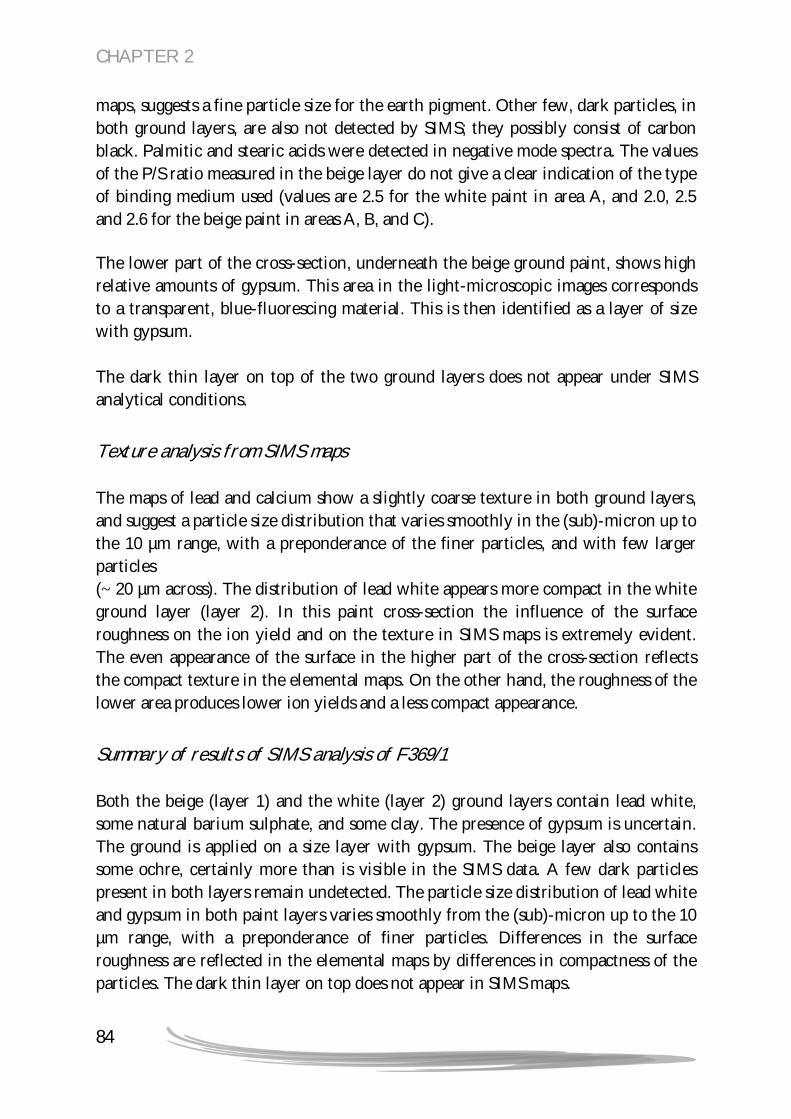
CHAPTER 2
84
maps, suggests a fine particle size for the earth pigment. Other few, dark particles, in both ground layers, are also not detected by SIMS; they possibly consist of carbon black. Palmitic and stearic acids were detected in negative mode spectra. The values of the P/S ratio measured in the beige layer do not give a clear indication of the type of binding medium used (values are 2.5 for the white paint in area A, and 2.0, 2.5 and 2.6 for the beige paint in areas A, B, and C). The lower part of the cross-section, underneath the beige ground paint, shows high relative amounts of gypsum. This area in the light-microscopic images corresponds to a transparent, blue-fluorescing material. This is then identified as a layer of size with gypsum. The dark thin layer on top of the two ground layers does not appear under SIMS analytical conditions.
Texture analysis from SIMS maps The maps of lead and calcium show a slightly coarse texture in both ground layers, and suggest a particle size distribution that varies smoothly in the (sub)-micron up to the 10 µm range, with a preponderance of the finer particles, and with few larger particles (~ 20 µm across). The distribution of lead white appears more compact in the white ground layer (layer 2). In this paint cross-section the influence of the surface roughness on the ion yield and on the texture in SIMS maps is extremely evident. The even appearance of the surface in the higher part of the cross-section reflects the compact texture in the elemental maps. On the other hand, the roughness of the lower area produces lower ion yields and a less compact appearance.
Summary of results of SIMS analysis of F369/1 Both the beige (layer 1) and the white (layer 2) ground layers contain lead white, some natural barium sulphate, and some clay. The presence of gypsum is uncertain. The ground is applied on a size layer with gypsum. The beige layer also contains some ochre, certainly more than is visible in the SIMS data. A few dark particles present in both layers remain undetected. The particle size distribution of lead white and gypsum in both paint layers varies smoothly from the (sub)-micron up to the 10 µm range, with a preponderance of finer particles. Differences in the surface roughness are reflected in the elemental maps by differences in compactness of the particles. The dark thin layer on top does not appear in SIMS maps.

CHAPTER 2
85
2.5 TECHNICAL DISCUSSION AND CONCLUSIONS With SIMS we were able to investigate the material composition and the textural characteristics of the paint layers in painting cross-sections. SIMS allowed analysis of both the pigment and the binding medium content of the paints, providing information on their spatial distribution within the paint layers. The distributions show a good match in terms of particle shape and position in the paint layer with light-microscopic, SEM-EDX, and -BSE images, allowing a direct comparison of the different image data sets. The combination of these characteristics enables us to identify and differentiate the different materials in the paint layers, and at the same time to examine the texture of the particulate materials individually. Both the compositional and textural characteristics are features that can potentially allow a discrimination of the different types of the paints. SIMS can be considered as complementary to SEM-EDX rather than a simple substitute. In fact each of the two techniques is able to distinguish two different elements or molecular fragments where the other technique may fail. In addition, in contrast to SEM, SIMS provides information on the organic fraction of the sample and probes only the upper 10 nm of the cross-section. In the paintings under investigation, we were able to detect and identify all the major components of the ground paints, lead white, calcium carbonate, gypsum, and barium sulphate. Barium sulphate is in its natural form, as it was found in association with strontium. SIMS data also show different grades of coarseness for the paint. For elements of higher detection efficiency, yields reflected the morphology of individual particles, provided that these are sufficiently large compared to the instrumental lateral resolution at the analytical conditions used. Tables 1 and 2 summarize the compositional information determined by SIMS in both the ground and the upper paint layer; the tables compare our results with the findings of the previous study of Hendriks and Geldof. Qualitatively we can distinguish between two types of ground formulations, one consisting of a simple mixture of lead white and calcium carbonate (F216a and F216b), and a second one consisting of a mixture of lead white, calcium carbonate or gypsum, and barium sulphate (F216d, F216e, F216f, F216j, F267, F294, F296). Calcium carbonate is found in samples F216a/1, F216b/1, F294/1, and gypsum in samples F216f/2, F216j/1, F267/2. There does not seem to be any calcium carbonate or gypsum in detectable amounts in sample F216e/1. It is also uncertain whether sample F216d/1 contains calcium carbonate, and whether sample F296/2 contains
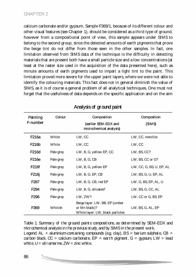
CHAPTER 2
86
calcium carbonate and/or gypsum. Sample F369/1, because of its different colour and other visual features (see Chapter 1), should be considered as a third type of ground, however from a compositional point of view, this sample appears under SIMS to belong to the second group, since the detected amounts of earth pigments that prove the beige tint do not differ from those seen in the other samples. In fact, one limitation observed from SIMS data of the technique is the difficulty in detecting materials that are present both have a small particle size and a low concentrations (at least at the raster size used in the acquisition of the data presented here), such as minute amounts of earth pigments used to impart a light tint to the paint. This limitation proved more severe for the upper paint layers, where we were not able to identify the colouring materials. This fact does not in general diminish the value of SIMS, as it is of course a general problem of all analytical techniques. One must not forget that the usefulness of data depends on the specific application and on the aim
Analysis of ground paint
Painting F-number
Colour
Composition
(earlier SEM-EDX and microchemical analysis)
Composition
(SIMS)
F216a White LW, CC LW, CC, menilite
F216b White LW, CC LW, CC
F216d Pale grey LW, B, G, yellow EP, CC LW, BS, CC?
F216e Pale grey LW, B, G, CB LW, BS, CC or G?
F216f Pale grey LW, B, G, yellow EP LW, CC, G, BS, U, EP, AL
F216j Pale grey LW, B, G, EP, CB LW, BS, G, U, EP, AL
F267 Pale grey LW, B, G, CB, red EP LW, G, BS, EP, AL, U
F294 Pale grey LW, B, G, silicates? LW, BS, G, CC, AL
F296 Pale grey LW, ZW? LW, CC or G, BS, EP
F369 Whitish Beige layer: LW, BB, EP (umber or Mn black)? White layer: LW, black particles
LW, BS, G, AL, EP
Table 1. Summary of the ground paints compositions, as determined by SEM-EDX and microchemical analysis in the previous study, and by SIMS in the present work. Legend: AL = aluminium-containing compounds (e.g. clay), BS = barium sulphate, CB = carbon black, CC = calcium carbonate, EP = earth pigment, G = gypsum, LW = lead white, U = ultramarine, ZW = zinc white.

87
Ana
lysi
s of
upp
er p
aint
Pain
ting
F-nu
mbe
r Co
lour
Com
posit
ion
(ear
lier S
EM-E
DX
and
m
icro
chem
ical
ana
lysis
)
Com
posit
ion
(SIM
S)
F216
a B
lue
LW, Z
W, P
B, E
P, V
E LW
, ZW
, EP,
VE,
AL
F216
b B
lue
LW, Z
W, P
B, U
, VE
LW, Z
W, A
L, U
F216
d G
reen
ish-b
lue
LW, Z
W, V
E, g
lass
/qua
rtz,
PB
LW, Z
W, E
P?
F216
e G
reen
ish-b
lue
LW, Z
W, V
E, P
B LW
, ZW
, AL
F216
j B
luish
-gre
en
LW, Z
W, P
B, V
E LW
, ZW
, VE
F267
D
ark
(thi
n la
yer)
V
I V
I
F294
B
lue
LW, V
I, V
E, C
o bl
ue?
LW, Z
W, C
, VI,
VE
F296
L
ight
blu
e LW
, B, C
o bl
ue, V
E, Z
Y, V
I Co
blu
e, L
W, C
C or
G, V
I, Cu
blu
e, V
E, E
P Ta
ble
2. Su
mm
ary
of t
he u
pper
pai
nt l
ayer
com
posi
tion
s, as
det
erm
ined
by
SEM
-ED
X an
d m
icro
chem
ical
ana
lysi
s in
the
pre
viou
s st
udy,
and
by S
IMS
in t
he p
rese
nt w
ork.
Leg
end:
AL
= a
lum
iniu
m-c
onta
inin
g co
mpo
unds
(e.g
. cla
y), B
S =
bari
um s
ulph
ate,
CC =
ca
lciu
m c
arbo
nate
, Co
blue
= c
obal
t bl
ue, C
u bl
ue =
cop
per
blue
, EP
= e
arth
pig
men
t, G
= g
ypsu
m, L
W =
lead
whi
te, P
B =
Pru
ssia
n bl
ue, U
= u
ltra
mar
ine,
VE =
ver
mili
on, V
I = v
irid
ian,
ZY =
zin
c ye
llow
, ZW
= z
inc
whi
te.
Tabl
e 3
(fol
low
ing
page
). Su
mm
ary
of b
indi
ng m
ediu
m a
naly
sis
in t
he g
roun
d pa
ints
by
SIM
S an
d G
C/M
S. F
or a
pur
e pl
ant
oil b
indi
ng
med
ium
the
P/S
rat
io i
s in
dica
tive
of
the
type
of
oil
(lins
eed
<2, w
alnu
t or
pop
py >
2.5).
The
C12,
C14,
and
C15
fatt
y ac
ids
are
char
acte
rist
ic m
arke
rs o
f an
imal
fat
s. Co
-occ
urre
nce
of C
12, C
14, C
15, C
16, a
nd C
18 r
evea
l tha
t a
mixt
ure
of p
lant
oil
and
anim
al f
at
wer
e us
ed. S
IMS
was
per
form
ed o
n di
ffer
ent
area
s of
pai
nt c
ross
-sec
tion
s. Th
e ta
ble
repo
rts
the
coun
ts f
or t
he p
eaks
of
fatt
y ac
ids.
The
qual
ity
of t
he m
aps
of C
16 a
nd C
18 f
atty
aci
ds w
as v
isua
lly e
valu
ated
(++
= ve
ry g
ood,
+ =
good
, +/-
= m
ediu
m, -
= p
oor,
--
= ve
ry p
oor)
. GC-
MS
was
per
form
ed o
n ad
diti
onal
sam
ples
of
thre
e of
the
gro
unds
. The
occ
urre
nce
of e
ach
char
acte
rist
ic f
atty
aci
d in
the
GC-
mas
s sp
ectr
a is
indi
cate
d w
ith
a (+
) sig
n.
CHAPTER 2

88
SIM
S G
C-M
S Fa
tty
acid
s (co
unts
) Pa
intin
g F-
num
ber
Sam
ple
code
A
rea
C12
(m/z
199
)C1
4 (m
/z 2
27)
C15
(m/z
241
)C1
6 (m
/z 2
55)
C18
(m/z
283
)
Qua
lity
of m
aps
Mix
ture
oil a
nd
anim
al
fats
?
P/S
Ratio
(C
16/C
18)
Sam
ple
code
Fa
tty
acid
s (C
12, C
14, C
15,
C16,
C18
)
Mix
ture
oi
l and
an
imal
fa
ts?
A
210
1025
10
53
6626
20
01
++
y -
B 21
5 11
37
1190
71
00
2084
++
y
- F2
16a
F216
a/1
C 16
678
577
850
6116
29++
y
-
A
22
59
27
612
287
--
2.
1 B
38
162
121
164
118
-
1.4
C 66
20
5 15
7 88
7 56
2 --
1.6
F216
b F2
16b/
1
D
2016
712
898
128
3-
3.5
F216
b/3
+, +
, +, +
, +
y
A
52
593
515
3078
11
74
+ y
- F2
16d
F216
d/1
B 75
631
672
3710
1469
+ y
-
F216
e F2
16e/
1 A
17
82
70
56
0 35
9 -
1.
6 F2
16e/
2 +,
+, +
, +, +
y
A
137
965
877
3185
19
26
+
1.7
F216
f F2
16f/2
B
114
711
599
2711
1678
+ 1.
6
A
87
657
607
3823
16
05
+
2.4
B 11
0 90
7 86
1 47
34
1959
+
2.
4 F2
16j
F216
j/1
C 91
652
619
3827
1649
+ 2.
3
A
68
194
179
1461
68
7 +/
-
2.1
B 10
4 21
2 31
1 17
71
845
+/-
2.
0 F2
67
F267
/2
A
6915
015
312
4862
4+ /
- 2.
0F2
67/3
+,
+, +
, +, +
y
F294
F2
94/1
A
86
41
0 56
7 42
29
1965
+
y -
A
73
27
4 44
8 77
5 44
1 -
1.
8 F2
96
F296
/2
B 75
225
416
622
330
- 1.
9
A
(whi
te)
147
652
526
3032
11
91
+/-
2.
5
A
(bei
ge)
164
444
265
2212
11
15
+/-
2.
0
B 31
6 82
7 28
35
4357
16
54
+/-
2.
6
F369
/1
F369
/1
C 29
290
178
848
2418
49+/
- 2.
6
CHAPTER 2

CHAPTER 2
89
of the study. We will see in Chapters 4 and 5 whether the data obtained by SIMS, and their quality, can be used for a quantitative comparison of the ground paints. Additional information obtained with other techniques and/or data analysis methods can be integrated in order to provide a more representative and discriminating set of features. Information on the binding medium of the ground paints obtained by SIMS and GC-MS is summarized in Table 3. The table reports the counts for characteristic peaks of fatty acids in SIMS mass-spectra. All paints are oil based as indicated by palmitic (C16) and stearic (C18) acids. The co-occurrence of the markers of animal fat sources C12, C14, C15, indicates that for some of the grounds that a non-pure oil medium was used. Addition of egg or milk derived products is possible, with the aim to make a more absorbent ground. GC-MS was also performed on additional samples of three of the grounds. In these grounds evidence of contributions from animal fat sources was observed by GC-MS but not by SIMS. Additional investigations would be necessary to exactly identify the cause of these differences. The following factors might be considered: differences in detection limits; probing by SIMS of the surface (~10 nm thickness) in contrast with the sample volumes analysed by GC-MS; the possibility with SIMS of considering a region of interest within the ground paint layer, while portions of other paint layers might be included in the paint sample analysed by GC-MS. A peculiar finding in one of the ground paints is that of a magnesium-rich variety of opaline silica, found only in few localities, called menilite. The discovery of menilite in the ground paint suggests that a suitable sedimentary rock itself is sometimes used directly in stead of mixing of separate additions or raw materials from pure sources as is the current wisdom (additional information is given in the Appendix to the this Chapter). This might be the case when a raw material is not a major paint component or when the raw material must be necessarily cheap. For example barite, clay minerals, iron oxides, and silica, which can be found as minor components in limestone deposits, might have been added unintentionally to the priming ground mass together with the calcium carbonate main component from limestone. Furthermore because of impurities, limestone and gypsum can exhibit a variety of colours and tints. Coloured and tinted grounds could be obtained by using less pure varieties of these materials, without the need of separate addition of colouring agents or pigments. We postulate that some colourmen in Paris in the late 19th century used suitable raw materials that they could get cheaply from local quarries or stone millers for use without much pretreatment except grinding to a suitable particle size.

CHAPTER 2
90
2.6 ACKNOWLEDGEMENTS The samples were provided by Ella Hendriks (Van Gogh Museum, Amsterdam). We thank Stefan Luxembourg and Liam McDonnell (AMOLF, Amsterdam) for technical assistance with SIMS instrumentation, and Katrien Keune (AMOLF) for assistance in the acquisition and interpretation of SIMS data specifically for paint cross-section samples. Jerre van der Horst (AMOLF) made the GC-MS measurements. Muriel Geldof (ICN, Amsterdam) is thanked for providing information on earlier investigations made on the samples. 2.7 REFERENCES VAN DER BERG, K.J., and Heeren, R., 1998. Secondary Ion Mass Spectrometry on paint cross-sections, Molart report 1995-98, p. 83. BOMFORD, D., Leighton, J., Kirby, J., and Roy, A., 1991. Art in the making: Impressionism, National Gallery London Publications, Yale University Press, New Haven and London. CALLEN, A., 2000. The art of Impressionism: painting technique & the making of modernity, Yale University Press, New Haven and London. CARLYLE, L., 2001. The artist’s assistant: oil painting instruction manuals and handbooks in Britain 1800-1900 with reference to selected eighteenth century sources, Archetype Publications, London. CARLYLE, L., Witlox, M. et al., 2005. HART project report. Report of the De Mayerne Programme project: Historically Accurate Reconstructions of Oil Paint and Painting Composites. DAMOUR, M.A., 1884. Essais chimiques et analyses sur la menilite. Bulletin Société Minéralogie de France, 7, p. 239-241. DEER, W.A., Howie, R.A., and Zussman, J. 1967. An introduction to the rock-forming Minerals, Longmans, London, p. 462-464.

CHAPTER 2
91
ENCYCLOPAEDIA BRITANNICA, 1992. ‘nodule’, The New Encyclopaedia Britannica, 15th ed., Encyclopaedia Britannica Inc., Chicago and London, vol. 8, p. 749. ENCYCLOPAEDIA BRITANNICA, 1992. ‘jasper, chert and flint, The New Encyclopaedia Britannica, 15th ed., Encyclopaedia Britannica Inc., Chicago and London, vol. 24, p. 199. FELLER, R., 1986. Barium sulphate - natural and synthetic. in Artists’ pigments: a handbook of their history and characteristics, National Gallery of Art, Washington, p. 47-64. GETTENS, R.J., and Stout, G.L., 1966. Painting materials – A short encyclopaedia, Dover Publications Inc., New York. HENDRIKS, E., and Geldof, M., 2005. Van Gogh’s Antwerp and Paris picture supports (1885-1888) reconstructing choices, ArtMatters Netherlands Technical Studies in Art, 2, p. 39-74. KEUNE, K., 2005. Binding medium, pigments and metal soaps characterised and localised in paint cross-sections, Ph.D. Thesis, University of Amsterdam, http://www.amolf.nl/publications/theses/. KEUNE, K., and Boon, J.J. 2004. Imaging secondary ion mass spectrometry of a paint cross-section taken from an early Netherlandish painting by Rogier van der Weyden, Analytical Chemistry, 76, p. 1374-1385. KEUNE, K., Ferreira, E., and Boon, J.J., 2005. Characterisation and localisation of the oil binding medium in paint cross-sections using imaging secondary ion mass spectrometry, Proceedings of the 14th Triennial Meeting of the ICOM Committee for Conservation in the Hague, The Netherlands, September 12-16, 2005. VAN LOON, A., Keune, K., and Boon, J.J., 2005. Improving the surface quality of paint cross-sections for imaging analytical studies with specular reflection FTIR and Static-SIMS, Conference Proceedings Art’05: 8th International Conference on Non-destructive Testing and Microanalysis for the Diagnostics and Conservation of the Cultural and Environmental Heritage, Lecce, Italy, 15-19 May, 2005. MARINO, B., Keune, K., Hendriks. E., and Boon, J.J., 2005. SIMS studies of the

CHAPTER 2
92
material aspects in grounds and paints in paintings by Van Gogh, Conference Proceedings Art’05: 8th International Conference on Non-destructive Testing and Microanalysis for the Diagnostics and Conservation of the Cultural and Environmental Heritage, Lecce, Italy, 15-19 May, 2005. PLESTERS, J., 1993. Ultramarine blue, natural and artificial, in Artists’ pigments: a handbook of their history and characteristics, Roy, A (Ed.), National Gallery of Art, Washington, p. 37-66. SCHILLING, M.R., and Khaijan, H.P., 1996. Gas chromatographic determination of fatty acid and glycol content of lipids I. The effect of pigments and aging on the composition of oil paints, Preprints of the 11th triennial meeting of the ICOM Committee for Conservation, Edinburgh, United Kingdom, 1, p. 242-247. VICKERMAN, J.C. et al., 2001. ToF-SIMS: Surface Analysis by Mass Spectrometry, Vickerman, J.C., Briggs, D. (Eds.), IM Publication and Surface Spectra Limited, West Sussex and Manchester, chapters 18-28.

93
to Chapter The ground paints under study, as already mentioned, are commercial preparations made in Paris. Many of the paint materials present in the grounds (calcium carbonate, gypsum, barite, menilite, clay) can be found in France. In particular, the Paris Basin itself is the most likely the source of these materials. It is therefore interesting to look into the geology and the mining activities of this area. In Chapter 2 (Section 2.4.1) we saw that one of the ground paint samples contains the menilite variety of chert. This finding is very interesting since, as will be explained in this Section, menilite points to Paris and the Paris Basin as likely sources of some of the materials used in the grounds under study, specifically calcium carbonate, gypsum, barite, and clay. It is therefore of interest to give a short account of the geology of the Paris Basin and its exploitation, within the framework of the urban development and of the activities of artists and colourmen in Paris.

APPENDIX to CHAPTER 2
94
A2.1 MENILITE, THE PARIS BASIN, AND PAINT MANUFACTURING AND TRADING
Menilite is the magnesium-rich variety of chert, which is a naturally occurring form of hydrous amorphous silica, or opaline silica. This mineral is interesting, as it is found in very few localities and occurs within a limited time frame in the area around Paris (see map in Figure 1). Menilite gained its name because it is found in Tertiary shale deposits in Ménilmontant (type locality)3, now in the XX arrondissement of Paris [Damour 1884]. In France it is found only in the Paris Basin, which covers the area of the Île-de-France4. The hills of Ménilmontant, Montmartre, Belleville, and Chaumont formed the centre of Paris’ gypsum mining activity in the 19th century (localities are shown Figure 1). In fact the Paris Basin is a rich source of limestone, gypsum, clay and sand. These deposits have been exploited throughout the centuries since the Celtic Parisii established the first settlements in the Ile de la Cité, which later became the heart of Paris5. All these local raw
Figure 1. Map of the area of Paris. The map shows the localities of the house of Van Gogh (1); the painters’ quarter of Montmartre (2); the main areas of mining activities in Paris in the 19th century (2, 3, 4, 5); and areas of occurrence of menilite (3, 5, 6, 7, 8, 9, 10).
3 www.segnitopals.net.au/main/scientific_12.html; www.mindat.org/min-9796.html; http://en.wikipedia.org/wiki/Menilite 4 Other localities are in Hungary, Germany, and Algeria (www.mindat.org). 5 www.paris-promenade.com

APPENDIX to CHAPTER 2
95
materials are also found in paints. In 19th century Paris was a very important and active artistic centre, and the trade of small colourmen next to large artists’ materials manufacturers was flourishing. Is therefore likely that Paris itself and its immediate surroundings were a source of materials for the colourmen. At the beginning of his stay in Paris in 1886, Van Gogh reproduced a number of views of the hill of Montmartre with its windmills6, close to Rue Lepic where Vincent and his brother Theo were living [Hulsker 1996]. These paintings show the conditions at that time in Montmartre, which was still a very rural and little urbanized area7. Montmartre, together with Ménilmontant and other villages in the surroundings of Paris were joined to the city only a couple of decades earlier in 1860, following a population expansion. Some of these areas, now in the XVIII, XIX, and XX arrondissement, were later colonized by artists, for living and for their artistic activities. Views of Montmartre made by Van Gogh reproduce a quarry along the slope of the hill, a testimony of the mining activities that were taking place in the area at that time (two of these landscape paintings are illustrated in Figures A.11-A.12 in Appendix A). A2.2 CHERT AND MENILITE Chert, like opal, originates for example from dissolved and remineralized siliceous sponge fossils, and occurs as reprecipitation of silica in nodules or bands in sedimentary rocks, such as limestone and shale deposits, where silica replaces the carbonate rock [Encyclopaedia Britannica 1992, vol. 8 and 15]. Minor constituents are usually aluminium, iron, magnesium, calcium, sodium and potassium in widely varying proportions. Most opals have MgO contents of less than 2%, while the menilite variety typically contains 7 to 8% of MgO [Webb and Finlayson 1987]. The microstructure of opal consists of amorphous silica spheres (200-500 nm diameter), which in common opal are irregular and varying in size, while in precious opal the perfectly uniform layered spheres diffract white light into its component colours producing its typical play of colour [Sanders and Darragh 1971]. Magnesium is more likely to be interstitial rather than substituting for silica, as
6 Two of these windmills were in Rue Lepic. One, still surviving, is the Blute-Fin, later known as the café-concert Moulin de la Galette, and the other was the Radet, of which now there is only a reproduction (source: www.vggallery.com). 7 Paris was officially enlarged by decree in 1860, from 12 arrondissement to the actual 20 arrondissement, to join its immediate surroundings, including the villages of Montmartre and La Chapelle (XVII arrondissement), Belleville, Chaumont and La Villette (XIX arrondissement), and Ménilmontant, Belleville, Charonne (XX arrondissement).

APPENDIX to CHAPTER 2
96
magnesium has a much larger radius and a lower charge than silicon or aluminium. The poorly ordered structure in the opal structure can accommodate ions of this size [Eitel 1964]. The occurrence of the chert variety menilite is very limited in space and time, so that it has been referred to as an exception among the various forms of silica [Cayeux 1929]. It was first found in 17878 and named as such in 1797. In France, menilite is found only in the Paris Basin in the Eocene magnesium-rich layers of marl and in the magnesite (magnesium carbonate, MgCO3) beds in the Saint-Ouen limestone deposit. Localities of occurrence of menilite include Ménilmontant, Buttes Chaumont, Villejuif, Argenteuil, plaine Monceau, plaine d’Ablon, and the Lambert quarry in Cormeilles-en-Parisis [Cayeux 1929, Lacroix 1962, Pormerol 1968]. A2.3 GEOLOGY OF THE PARIS BASIN The Paris Basin occupies the centre of the northwestern part of France and is one of its major geological regions (the extension of the Paris Basin is shown in Figure 2). Its paleostratigraphy is the result of a series of marine transgressions and regressions (sea level changes relative to land) that took place during the Tertiary period. The resulting sediments and detrital materials layered over chalk beds formed in the Mesozoic consist of a series of marls (impure limestone with varying amounts of clay), limestone, clay, and gypsum deposits in alternations of marine, lagonal, and lacustrine environments [Pormerol and Feugueur 1968, Pormerol and Feugueur 1986]. The sediments of the Paris Basin have been intensively exploited since antiquity to extract the clay, sandstone, limestone, and gypsum, mainly to produce construction materials but also for other purposes. For example gypsum was extracted to make plaster of Paris. The depth of mining extended over several tenths of meters. Even presently there is an open pit mine with a maximum of 110 m depth at Cormeilles-en-Parisis just across the route periferique (belt way). Paris and the villages in the Ile de France were built using local construction material. The exposed face of the open pit Lambert quarry in Cormeilles-in-Parisis9, situated in the Île-de-France at 20 km northwest of Paris, shows the stratigraphy of the sediments formed between the late Eocene (Ludian) and the early Oligocene (Stampian) [Pormerol and Feugueur 1968]. The stratigraphic section of the Lambert 8 However it was confused with pitchblack, and called pechstein de Mesnil-Montant. 9 This quarry, opened in 1820 and still active, is the largest open pit in Europe. Gypsum, limestone, clay, and sand are extracted to produce plaster, bricks, lime, cement, glass and for other uses.

APPENDIX to CHAPTER 2
97
Figure 2. Extension of the Ludian marls, limestone and gypsum deposits in the Paris Basin (reproduced after Pormerol and Feugueur 1986).
Figure 1. Stratigraphic section of the Lambert quarry (Cormeilles-en-Parisis). At present only the layers above and including the 2nd gypsum mass (layer 9) are exposed. The stratigraphic structure underneath this layer is reconstructed by comparison with various outcrops along the Seine river in the area (source: Pormerol and Feugueur 1968 and 1986).

APPENDIX to CHAPTER 2
98
quarry is shown in Figure 3, starting from the Mesozoic chalk bed (layer 1) on which the Tertiary sediments and detrimental materials accumulated. The lowest visible layers (9-11, ~ 28 m thick) are the uppermost of a series of alternating gypsum deposits and attapulgite-containing marls (6-11). Attapulgite is a magnesium-rich type of clay. These sediments formed in lake environments in the late Eocene (Ludian). Detrital gypsum is transported by rivers from Lorraine in the east. The marl d’entre-deux-masses (10) consists of layers of green and yellow marls and layers of pinkish gypsum. These magnesium-rich marls also contain whitish menilite. Menilite was found also in the magnesite beds in the Saint-Ouen limestone deposit (layer 4). [Cayeux 1929, Lacroix 1962, Pormerol 1968]. The 17m-thick first and youngest gypsum mass (11) is the same layer that lies below the hills of Montmartre, Belleville, Chaumont, and Menilmontant, which formed the centre of the mining activity in Paris in the 19th century. A heterogeneous ensemble of layers of different origins called marnes (marls) supragypseuses (12-17, ~28 m thick), deposited over the gypsum deposits, formed between the late Eocene (Ludian) and the early Oligocene (Stampian). These layers consist of marls intercalated with gypsum and limestone deposits, and exhibit different colourations because of different types and degrees of impurities. The clay is the attapulgite form in layers 12 and 13, illite (mica) in layer 14, and kaolinite in layer 15. A2.4 OBSERVATIONS ON THE CHARACTERISTICS OF OTHER
MATERIALS FOUND IN PAINTS
Calcium carbonate Calcium carbonate is found in limestones of biogenic and non-biogenic origin. They are abundant below the Tertiary deposits from the Paris Basin. Cretaceous chalk for example outcrop in the Boulonnais between Normandy and Calais. For chalk the source of calcium carbonate are marine nanofossils of coccolhitophorids. Other calcium carbonate secreting organisms are microscopic foraminifera, corals and mollusc shells. Non-biogenic limestones are formed as precipitates due to physico-chemical conditions in ocean water. Limestones are white or almost white when pure. They exhibit different colours however when they contain impurities, such as clay, sand, iron oxide, and other materials. Limestone may contain variable amounts of silica in the form of chert or flint, as well as varying amounts of clay, silt, and sand.

APPENDIX to CHAPTER 2
99
Gypsum Gypsum forms by the evaporation of seawater, for example in shallow marine basins. Gypsum is white when pure, but often coloured in white, grey, yellow, brown, or pink. The Eocene gypsum found near Paris is deposited by rivers that eroded gypsum deposits elsewhere.
Clays Clays are sediments composed predominantly of hydrous magnesium-aluminium silicate minerals. Because of their small particles size, clay layers are only formed in low energy environments. Most clay minerals are deposited as preexisting mineral matter transported by rivers. Clay occurs as impurity in limestone (abundant in marls), and fine-grained sandy deposits.
Barite Barite is the natural source of barium sulphate and the most common barium mineral. It is commonly found as a gangue mineral in metallic ore deposits, but it may also occur as lenses or replacement deposits in sedimentary rocks. Barite is generally pure BaSO4, however barium can be replaced by strontium in a continuous solid solution series from barites to celestine (SrSO4). Barites of this series with a preponderance of barium are called strontiobarites [Deer 1967]. In the process of making artificial barium sulphate a very pure product is obtained and most of the impurities are eliminated [Feller 1986]. Therefore, strontium can be used as an indicator of natural barium sulphate in paints and to discriminate different sources of the natural mineral [Marino et al. 2005]. In France barite can be found in many localities, including Tertiary clay deposits of the Paris Basin, where celestite is abundant in some sediments. In the Paris Basin nodules of celestite were found in Montmartre in the marls between the haute masse and the third mass of gypsum (layers 11 and 7 in Figure 3), in Romainville in the white marls (layer 13), and most abundantly in Menilmontant and Belleville in the layers of Cyrena clay and of green marl (layers 14 and 15) [Lacroix 1962, 4th vol.].

APPENDIX to CHAPTER 2
100
A2.5 FINAL COMMENTS The discovery of the rather peculiar presence of menilite in the paint used for priming suggests that a suitable sedimentary rock itself is sometimes used directly in stead of mixing of separate additions of raw materials from pure sources as is the current wisdom. This might be the case when a raw material is not a major paint component or when the raw material must be necessarily cheap. For example barite, clay minerals, iron oxides, and silica, which can be found as minor components in limestone deposits, might have been added unintentionally to the priming ground mass together with the calcium carbonate main component from limestone. Furthermore because of impurities, limestone and gypsum can exhibit a variety of colours and tints. Coloured and tinted grounds could be obtained by using less pure varieties of these materials, without the need of a separate addition of colouring agents or pigments. We postulate that some colourmen in Paris in the late 19th century used suitable raw materials that they could get cheaply from local quarries or stone millers for use without much pretreatment except grinding to a suitable particle size. And even those size fractions could have been a spinoff from another industrial application. A2.6 ACKNOWLEDGEMENTS We are grateful to Prof. Patrick de Wever (Muséum National d’Histoire Naturelle, Departement Histoire de la Terre, Géologie, Paris) for providing useful information on menilite and barite-celestite in France.

APPENDIX to CHAPTER 2
101
A2.7 REFERENCES CAYEUX, L., 1929. Les roches sédimentaires de France, Paris, Imprimerie Nationale. DAMOUR, M.A., 1884. Essais chimiques et analyses sur la menilite. Bulletin Société Minéralogie de France, 7, p. 239-241. DEER, W.A., Howie, R.A., and Zussman, J. 1967. An introduction to the rock-forming Minerals, Longmans, London, p. 462-464. EITEL, W., 1964. Silicate science, Vol. 1, Silicate structures, Academic Press, New York. FELLER, R., 1986. Barium sulphate – natural and synthetic. Chapter in Artists’ pigments: a handbook of their history and characteristics, Cambridge University Press, National Gallery of Art, Washington, p. 47-64. HULSKER, J., 1996. The new complete Van Gogh. Paintings, drawings, sketches. Revised and enlarged edition of the catalogue raisonné, Meulenhoff, J.M., and Benjamins, J. (Eds.), Amsterdam and Philadelphia. LACROIX, A., 1962. Minéralogie de la France et de ses anciens territories d’outre-mer, 3rd and 4th vol., Librairie Scientifique et Technique Albert Blanchard, Paris. MARINO, B., Keune, K., Hendriks. E., and Boon, J.J., 2005. SIMS studies of the material aspects in grounds and paints in paintings by Van Gogh, Conference Proceedings Art’05: 8th International Conference on Non-destructive Testing and Microanalysis for the Diagnostics and Conservation of the Cultural and Environmental Heritage, Lecce, Italy, 15-19 May, 2005. PORMEROL, C., and Feugueur, L., 1968. Guide géologique régionaux: Bassin de Paris Ile-de-France, Masson & Cie Éditeurs. PORMEROL, C., and Feugueur, L., 1986. Bassin de Paris, Ile-de-France, Pays de Bray, 3rd ed., Masson. SANDERS, J.V., and Darragh, P.J., 1971. The microstructure of precious opal, The Mineralogical Record, 2(6), p. 261-268.

APPENDIX to CHAPTER 2
102
WEBB, J.A., and Finlayson, B.L, 1987. Incorporation of Al, Mg, and water in opal-A: evidence from speleothems, American Mineralogist, 72, p. 1204-1210.

Quantitative colour analysis of ground paints
in paint cross-sections
He said, ‘What are field colorings, Gladia?’ ‘An art form’, she said.
... They entered a room that burst with light. It glowed in every corner
and every color.... The goblets of light sat on embracing pedestals. They were living geometry, lines and curves of color,
... One finger moved, describing half curve over smoothness. A bar of deep yellow
grew and slanted obliquely across the air above. The finger inched backward a fraction and the light grew slightly less deep in shade.
Isaac Asimov, ‘The naked sun’

CHAPTER 3
104
3.1 INTRODUCTION One of the main characteristics of paint is evidently colour. The colour of each paint layer including that of the ground paint has an impact on the final appearance of a picture. In some of his paintings Van Gogh used the colour of the ground paint itself is as a pictorial element, by leaving it exposed in between brushstrokes of the overlying paint layers [Hendriks and Geldof 2005]. The surface colour of the ground is one of the discriminating features that are used in comparative investigations, for example to assist in establishing a chronology or even proving authenticity of paintings [Hendriks 2006, Hendriks and Geldof 2005, Hendriks and van Tilborgh 2001]. Often however, it is hard to make a valid assessment of the ground colour, which may be exposed as an extremely small area and largely masked by paint layers on top, or distorted by accumulated grime and restoration materials, Additionally, perception is affected by the colour of surrounding areas. The uncertainty of visual examination is extremely large, and instrumental measurements should be used under controlled and reproducible conditions [Berns 2000]. However, often the assessment of the colour is made by qualitative visual examination, performed under uncontrolled illumination and viewing conditions, and in separate examination sessions for the different paintings. Equally, comparison of ground samples may prove inconclusive, since it is uncertain whether slight variations simply reflect the inhomogeneous character of hand-mixed paints, or real differences in paint formulation.

CHAPTER 3
105
The work presented here turns to a different approach, exploring the potential of classifying ground or paint cross-sections based on their colour content in light-microscopic images. Examination the colour of grounds in paint cross-section is particularly advantageous when there is no or very little paint surface exposed. Although uncomplicated, a light-microscopic image nevertheless contains information about the colours and their distribution in a cross-section, information that is useful and immediately recognizable by eye. Even though a full characterization of colour is provided by visible-light spectroscopy, the microscope is a tool available to most conservators or conservation scientists. For the analysis and comparison of colour images, there is a large number and variety of methods and algorithms in the field of pattern recognition and image analysis, with applications ranging from remote sensing to content-based image retrieval systems from databases. Colour histograms provide a simple and good characterization of images and are therefore extensively used in image-retrieval techniques. Stricker and Swain [1994] showed that the histogram space is sufficiently large to differentiate a large number of image histograms. Swain and Ballard [1991] used colour histogram to characterize images and developed the histogram intersection method. Hafner et al. [1995] proposed a class of quadratic form distance functions for evaluating the similarity of image histograms. The most known image retrieval system, the QBIC system developed by IBM, makes use of colour histogram quadratic distance for queries of large image databases based on colour content [Faloutsos et al. 1994, Flickner et al. 1995]. In the art field, the QBIC system is employed by the web site of the Hermitage museum in St Petersburg for searching archives of digital images of works of arts. In this Chapter we explore the performance of a method of classification based on histogram comparison by histogram quadratic distance and cluster analysis. The aim is to attempt a classification based on the colour content of light microscopic images, to determine whether the chosen colour representation is suitable for detecting sample differences in the visible spectrum (400-700 nm), and to see how well it compares to the earlier qualitative classification. This classification is made on the basis of technical investigations utilising the pigment mineral composition of the grounds but ignoring particle size distribution and texture. The technique is applied to a series of images of cross-sections taken from of a group of ten paintings by Van Gogh, painted on ready-primed supports. The colour data were acquired under standardized conditions. The application is conceptually simple but to our knowledge new in the application to the field of paint studies. In general, we see other potential applications of the method in painting studies.

CHAPTER 3
106
3.2 MATERIALS
3.2.1 SAMPLES The samples under investigation are paint cross-sections taken from a group of ten paintings of Van Gogh’s Paris period (1886-1887), which were discussed in Chapters 1 and 2.
3.2.2 ACQUISITION OF LIGHT-MICROSCOPIC DIGITAL IMAGES The setup for the acquisition of digital images consists of a Leica DMR microscope attached to a NIKON DXM1200 8-bits colour digital camera, driven by Eclipse Net acquisition software. The illumination is provided by an internal tungsten-halogen lamp (12 V, 100 W, 3400 K colour temperature). The microscope was operated in reflection mode, dark field, at 20x magnification. In order to achieve a consistent reproduction of colours and a meaningful comparison, we shielded the microscope from the influence of external and non-reproducible light sources, and used the internal illumination under standard and reproducible conditions. The illumination intensity was set, through a voltage control knob, to a fixed value, which was used consistently throughout the acquisition. The illumination intensity was reduced through the use of a N/4 neutral density filter placed within the optical pathway. As all images were acquired in the same day, there are no effects of change in the colour temperature due to aging of the lamp. In addition, by manual adjustment of the colour balance of the camera, made by setting the white point on a piece of white laboratory filter paper, we minimized the colourcast introduced by the camera and the microscope. In order to be able to compare meaningfully the colours of different images, all images were acquired consistently at the same exposure time, which was chosen in order to not have colour saturation, and therefore loss of information, in any of the paint areas of interest. All images were acquired by setting unit gain, unit gamma, and zero offset in the acquisition software control panel. Depending on the size, one or two images were acquired for each cross-section (see images I-XV in Figures 3 and 4). Finally the images were saved as uncompressed TIFF files, as any alteration introduced by a non-loss-less compression algorithm cannot be accepted when performing a quantitative analysis.

CHAPTER 3
107
3.2.3 DATA ANALYSIS The images were imported in Matlab (version 6.5, The Mathworks, Inc.) and analysed with software developed by Beatrice Marino at the FOM-AMOLF Institute in Amsterdam. Image processing and analysis was performed on an Acer TravelMate 800 laptop computer with an Intel Centrino 1.6 GHz, 1 GB Level 2 cache processor and 768 MB RAM, Windows XP OS, with reasonable computational effort. 3.3 METHOD OF COLOUR COMPARISON IN DIGITAL
IMAGES In this Section we present the methodology adopted to compare digital images on the basis of colour in a quantitative fashion. To this end, we first need a suitable representation of the colour feature of an image, and then a definition of measure of similarity between the colour representations of two images. In this work we use the histogram to describe the colour feature of an image, and the histogram quadratic distance to define a measure of similarity. The classification is made by hierarchical clustering algorithms. A scheme of the method is illustrated in Figure 1 (the figures of this Chapter can be found at p. 117-122). We first illustrate the concepts of colour and of colour histogram in digital images.
3.3.1 COLOUR IN DIGITAL IMAGES AND HISTOGRAM OF AN IMAGE An image captured by a digital device such as a CCD camera consists of an array of discrete varying brightness values in successive rectangular blocks called pixels. In colour CCD cameras the detector is equipped with miniature red, green, and blue (RGB) absorption filters, fitted in front of the sensor elements, which act as the three colour primaries. This results for each image pixel in the image in three independent brightness values, one for each primary colour. Each colour in the image is then the result of the combination of these three primary colours according to additive colour mixture rules. Mathematically, this is expressed as:
bbggrrc cccˆˆˆ ++=
r or cr = (rc, gc, bc), (1) where r , g , and b are the primaries, cr is a colour, and rc, gc, and bc are the colour coordinates of colour cr in the colour space defined by r , g , and b . A visualization of the formation of colours in the RGB space is represented in Figure 2. Most

CHAPTER 3
108
cameras can distinguish 256 different shades of brightness for each colour channel, whose combination results in a colour space of about 16 millions of different colours. The histogram provides a convenient representation of a digital image by indicating the relative population of pixels for each colour, or in simpler words, the distribution of colours in the image. In formulas, for an image I made of P pixels and M possible different colours, the histogram H is defined as:
∑= ⎪⎩
⎪⎨
⎧ ==
P
p
mcpImH
1 otherwise 0
)( if 1 )(
r
for every m∈[1, M] (2)
where p is an index scanning across all pixels in the image, and mcr a colour in the colour space, with index m∈[1, M].
3.3.2 MEASURE OF SIMILARITY BY HISTOGRAM QUADRATIC DISTANCE A measure of similarity is expressed numerically by defining a distance between objects, which in this case are colour histograms. Since the computational time to extract and compare histograms increases significantly with the number of different colours, we first have to reduce the number of different colours by sampling down the images uniformly across the colour space. A reasonable computational time was achievable by reducing the total number of possible colours from the original number of about 16 millions down to 4096. Despite the strong reduction, the reproduction of colours of the cross-sections in the original image is quite faithful, and was considered adequate to our needs (Figure 5). For each image we extracted the colour histogram from a region of interest traced within the ground paint layer. In the images of the extra sample F396/1, which has two ground layers, we made one selection that included both layers, and two separate selections for the two layers. In order to test the robustness of the method, we also considered the histogram of the area of the blue paint layer in F269/2, for a total of 19 selections (see images 1-19 in Figures 3 and 4, and in Table 1). The histograms were normalized by the number of pixels of the corresponding selections, in order to eliminate any influence from the size of the selection:
)()()(
mHmHmh = , so that 1)(
1=∑
=
M
mmh . (3)

CHAPTER 3
109
The distance d(h, g) between two histograms h and g was then calculated according to the formula of the histogram quadratic distance:
∑∑= =
−⋅⋅−=M
m
M
mmm mgmhamgmhghd
1 111,00
0 1
10))()(())()((),( . (4)
The weights
10 ,mma attempt to express the perceptual similarity between any two different colours m0 and m1. For example, this measure can recognize orange images as similar to red images, and a half-red/half-blue image as quite different from an all-purple one. According to Hafner et al. [1995] this method ‘more closely corresponds to human judgment of colour similarity’. It makes sense to express
10 ,mma in terms of the distance
10 ,mmd between colour m0 and m1, normalized with respect to the maximum distance:
)(max1
1010
10
10,,
,,
mmmm
mmmm d
da −= , (5)
where
10 ,mmd is taken as the Euclidean distance in the RGB space. The distance formula therefore reduces to the following form:
∑∑= =
−⋅⋅−−=M
m
M
m mmmm
mm mgmhd
dmgmhghd
1 111
,,
,00
0 1 1010
10 ))()(()(max
))()((),( . (6)
We then compared the histograms in all possible pairs and finally obtained a table of mutual distances between images. From this table it is possible to see how images group in clusters of similar images by applying hierarchical cluster analysis methods, which are explained below.
3.3.3 CLASSIFICATION BY HIERARCHICAL CLUSTERING METHODS Cluster analysis is a useful technique for finding clusters or classes of objects that are similar to each other with respect to certain characteristics [Duda et al. 2000, Matlab documentation]. As mentioned above a measure of similarity is expressed numerically by defining a distance between objects. The more similar the objects, the smaller the distance and vice versa. Geometrically, cluster analysis corresponds to identifying clusters of objects that are close according to the definition of distance

CHAPTER 3
110
adopted. Hierarchical cluster analysis is an unsupervised classification method that does not require a priori knowledge of the number of clusters or of the initial partitions. Hierarchical clustering operates in a series of steps as follows. At each step the operator searches for the two objects whose distance is the smallest. These two objects are considered as belonging to the same cluster. Then new distances between the newly formed cluster and the other objects are calculated, according to a certain criterion. Different criteria can be used. The next cluster is formed by using the new set of distances, and the process is repeated until all observations are merged in one cluster. At each step new clusters are formed, or existing clusters are enlarged by adding other objects or by merging two separate clusters into a single one. Different hierarchical clustering methods are based on different criteria for calculating the distances between clusters. The methods considered here are single linkage, complete linkage, and average linkage. With the single-linkage method, the distance between two clusters is defined as the distance between the two closest objects in the two clusters:
)),((min),(, sjriji
xxdsrdist = , I = 1, …, nr , j = 1, …, ns (7)
where xri and xsj are the ith and the jth objects in clusters r and s, and nr and ns are the number of objects in clusters r and s. With the complete-linkage method, the distance between two clusters is determined by the two most distant objects in the two clusters:
)),((max),(, sjriji
xxdsrdist = . (8)
The complete-linkage method identifies compact clusters in which the observations are very similar to each other. In the average-linkage method, the average distance is considered:
∑∑= =
=r sn
i
n
jsjri
sr
xxdnn
srdist1 1
)),((11),( . (9)
The result of the clustering process is represented by a dendrogram, which is a tree-like structure showing how objects are grouped. The lengths of branches in the dendrogram represent distances between clusters. By choosing a height along the vertical axis of the dendrogram, and moving along the number of lines that are

CHAPTER 3
111
crossed, each line represents a group that was identified during the clustering process. The branches of the dendrogram that spread out below the line represent the observations in that group. The cluster solution is found by looking for a large gap in the distances between clusters. 3.4 DISCUSSION OF THE CASE STUDY:
GROUNDS IN PAINTINGS BY VAN GOGH In this Section we discuss the application of the method to the ground paints in paintings by Van Gogh (see Chapters 1 and 2). In Figure 6 (next page) two series of dendrograms show the results of cluster analysis made on the results of histogram comparison. The numbers identifying the images (as in Figures 3 and 4, and in Table 1) are listed on the horizontal axis and the vertical axis represents the distances between the centroids of the clusters. The interpretation of the clustering solution is summarized in Table 2 and discussed below. The results obtained from the different clustering methods are consistent with each other. The most evident result is how the blue paint layer (selection 15 from F296/2) is recognized immediately as being very much different from the other paint layers, which are white or off-white. The ground paint layers are classified in two main clusters. One of the two originally recognized subgroups of the grey grounds is identified as such (selections 11-14, from images of F267/2, F294/1, and F296/2). The colour of the ground paint in F216b/1 (selections 3-4) seems more similar to that of the grey grounds of F267/2, F294/1, F296/2 (selections 11-14), rather than to the others. In comparison, the other grey grounds in F216d/1, F216e/1, F216f/2, F216j/1 appear lighter and more similar to the ground colour of F216a/1, and form a separate cluster. Re-examination of the colour of the ground paint surface showed that in painting F267/2, F294/1, and F296/2 it appears slightly darker than in the other paintings. The two images of white on beige grounds in F369/1 would seem to fall between the two categories, with a higher similarity to the lighter grounds. In addition, the complete-linkage method clustered all the four selections as an individual subset separated from the white and grey grounds. It can also be noticed that images of different portions of the same ground are not necessarily the two most similar in a cluster (selections number 1-2, 3-4, 5-6, 9-10, and 11-12). Yet this does not necessarily imply a poor performance of the method, instead it reflects the variability of colour within the same paint. A visual examination of the colour in the images would suggest that the colour-based classification is correct. Figure 7 8 shows 3D visualizations in the RGB space of

CHAPTER 3
112
the colour histograms of all the ground paint layer images. In this type of visualization, each unique colour present in the image is represented by a circle of the same colour, whose position in the space is determined by its primary colour coordinates, and whose size is proportional to the frequency of occurrence of the colour in the image. Visual examination of the histograms also indicates that the distinction between the two identified groups of ground paints is based on differences in brightness. The colours of the particles in the grounds are in fact mainly distributed along the black-white axis. Slight tint differences, which distribute off this main direction of distribution, seem to have a low impact on the classification. This phenomenon for example causes the images of the white on beige ground to exhibit a strong similarity to the lighter grounds. Similarly, the few or small dark-coloured particles that are visible in the cross-section do not have a noticeable impact on the classification because of their small contribution to the coloured cross-section area compared to the light-coloured materials. These small or few black or dark coloured particles contribute little in coloured paint cross-section area, but are very striking for the human eye. In this way an occasional particle will get a very high discriminating weight in a qualitative subjective classification.
a b c
d e f
Figure 6. Dendrograms resulting from cluster analysis performed with the single-linkage (a, d), complete-linkage (b, e) and average-linkage (c, f) methods. Dendrograms a, b, and c are originated from cluster analysis on all the grounds under study, with the addition of selections in an extra ground sample and of a blue paint layer. Dendrograms in d, e, and f refer to a dataset limited to the ground paint layers under study only. The classifications and the numbering are reported in Table 2 (next page).

CHAPTER 3
113
Classification of
light-microscopic images
Sample
code
Image
selection number
Selection (layer)
Qualitative
classification
Single linkage
Complete linkage
Average linkage
F216a/1 1 ground 1 1 1 1
F216a/1 2 ground 1 1 1 1
F216b/1 3 ground 1 2 2 2
F216b/1 4 ground 1 2 2 2
F216d/1 5 ground 2a 1 1 1
F216d/1 6 ground 2a 1 1 1
F216e/1 7 ground 2a 2 2 2
F216f/2 8 ground 2a 1 1 1
F216j/1 9 ground 2a 1 1 1
F216j/1 10 ground 2a 1 1 1
F267/2 11 ground 2b 2 2 2
F267/2 12 ground 2b 2 2 2
F294/1 13 ground 2b 2 2 2
F296/2 14 ground 2b 2 2 2
F296/2 15 blue paint - 3 3 3
F369/1 16 whole ground (two layers)
- 1 1 1
F369/1 17 beige ground - 1 1 1
F369/1 18 white ground - 1 1 1
F369/1 19 beige ground - 1 1 1
Table 2. Summary of the classifications of the ground paints. The qualitative classification was made by examination of support, paint surface, and paint cross-sections. The quantitative classification was made separately on the basis of the colour of the ground paints in light-microscopic images of paint cross-sections. The numbers correspond to classes as follows. Qualitative classification: 1 = white grounds, 2a = grey grounds, batch A, 2b = grey grounds, batch B. Colour: 1 = light grounds, 2 = grey grounds.

CHAPTER 3
114
3.5 CONCLUSIONS In this Chapter we made a quantitative classification of ground paints in ready-primed carton supports from paintings by Van Gogh on the basis of their colour content. The application is conceptually simple but to our knowledge new in the application to the field of painting studies. The obtained classification partially follows a previous subjective classification, made on the basis of traditional technical investigational criteria that include qualitative information about the surface colour and the material composition of the paints (see Chapter 1). Despite the differences, the two classifications complement each other, since they were obtained from different types of data. One aspect to bear in mind is that the colour of paint in a cross-section and the colour of the paint surface are related in a complex way, which is the result of the integration of various light absorption, transmission and scattering interactions within the paint layer [Völz 2001]. Therefore paints that appear macroscopically similar might differ at the microscopic scale. For example relatively few dark particles in a light matrix may produce the same surface colour as a layer that is more uniformly tinted at the microscopic level. Colour is related to composition and compound texture of the paint materials, which have different optical behaviours. Paints of different formulations might in fact still be similar in terms of their colour component, but conversely, similar compositions do not necessarily translate in similar colours. For a painter the colour of the ground is a decisive factor irrespective of how this colour has been achieved by the colourman preparing the preprimed canvas. For the analyst of paintings colour is just one factor to consider in questions on the authenticity of paintings or the similarities in material composition, for reasons of understanding the painting production process or the historical sequence of the works. The results obtained show that the method has potential, and seems promising for the application to colour-specific case studies. One of the potential advantages of the approach is that it can handle a large number of samples in a relatively short time (compared to for example a detailed analytical comparison of each sample). Further developments of the algorithms might also include spatial information as described by Ennesser and Medioni [1995], and by Pass et al. [1996]. Although full characterization of colour is obtained by visible-light spectroscopy, the work presented here shows that RGB digital images prove to be a valid alternative when a visible spectrometer is not available. The advantage of the chosen colour representation is that it can be adopted by conservators or conservation scientists, since a digital camera and microscope set-up is easily accessible. The development and use of an appropriate set of calibration standards for use in

CHAPTER 3
115
microscopy would allow the comparison of images acquired in different sessions or different set-ups. Considering this objective it would be advisable to work in perceptually uniform colour spaces such as CIELab and CIELuv, which have been especially developed to measure colour differences [Berns 2000]. In a general sense it seems to open new possibilities for relating colour measurements in paint cross-sections to the colours actually seen on the paintings themselves. Also it would seem useful to study gradients of discolouration in paint cross-sections, such as the darkened surfaces of chrome yellow and red lead paints, or the faded surfaces of red lake paints. Interesting aspects to investigate are for example the measurement and similarity/difference of degrees of discolouration in paints, and the assessment of the visual impact of the depth of degree of discolouration on the paint surface. 2.8 ACKNOWLEDGEMENTS The samples were provided by Ella Hendriks of the Van Gogh Museum in Amsterdam. The histogram visualizations were generated in ImageJ10 with the 3D Color Inspector plugin by Kai Uwe Barthel of the University of Applied Sciences in Berlin. 2.9 REFERENCES BERNS, R.S., 2000. Billmeyer and Saltzman’s Principles of color technology, 3rd ed. Wiley Interscience. DUDA, R.O., Hart, P.E., and Stork, D.G., 2000. Pattern Classification, 2nd ed. Wiley Interscience. ENNESSER, F. and Medioni, G., 1995. Finding Waldo, or focus of attention using local color information. IEEE Trans. Pattern Anal. Machine Intell. 17(8), p. 805-809. FALOUTSOS, C., Equitz, W., Flickner, M., Niblack, W., Petkovic, D., and Barber, R., 1994. Efficient and effective querying by image content. Journal of Intelligent Information Systems. 3(3/4), p. 231-262. http://citeseer.ist.psu.edu/faloutsos94efficient.html
10 Available for free download at http://rsb.info.nih.gov/ij/

CHAPTER 3
116
FLICKNER, M. et al., 1995. Query by image and video content systems: The QBIC system. IEEE Comput. 28(9), p. 23-32. HAFNER, J., Sawhney, H.S., Equitz, W., Flickner, M., and Niblack, W., 1995. Efficient color histogram indexing for quadratic from distance functions. IEEE Trans. Pattern Anal. Machine Intell. 17(7), p. 729-736. HENDRIKS, E. 2006. Van Gogh’s working practice; a technical study, and Developing technique and style, essays in: Hendriks, E., and van Tilborgh, L., In relation to Van Gogh; a technical and art historical study of his Antwerp and Paris paintings in the Van Gogh Museum, PhD dissertation, Faculty of Humanities, University of Amsterdam (to be defended on 15th November 2006). HENDRIKS, E., and Geldof, M., 2005. Van Gogh’s Antwerp and Paris picture supports (1885-1888) reconstructing choices, ArtMatters – Netherlands Technical Studies in Art, 2, p. 39-74. HENDRIKS, E., and van Tilborgh, L., 2001. Van Gogh’s ‘Garden of the asylum’: genuine or fake?, The Burlington Magazine, p. 145-155. MATLAB documentation available at www.mathworks.com. PASS, G., Zabih, R. and Miller, J., 1996. Comparing images using color coherence vectors. Proc. ACM Multimedia ’96, p. 65-73. STRICKER, M. and Swain, M., 1994. The capacity of color histogram indexing. Proc IEEE CVPR’94, p. 704-708. SWAIN, M.J. and Ballard, D.H., 1991. Color Indexing. Internat. J. Computer Vision 7(1), p. 11-32. VÖLZ, H.G., 2001. Industrial color testing: fundamentals and techniques, 2nd ed., Wiley-VHC.

FIGURES of CHAPTER 3
117
Figure 1. Scheme of the method for quantitative comparison of colour from light-microscopic images.

FIGURES of CHAPTER 3
118
Figure 2. All colours in a digital image are represented by different combination of three primary colours (red, green, and blue in the RGB space) according to additive colour mixing rules.
Sample
code Image
selection number
Image number
Selection (layer)
1 I ground F216a/1
2 II ground
3 III ground F216b/1
4 IV ground
5 V ground F216d/1
6 VI ground
F216e/1 7 VII ground
F216f/2 8 VIII ground
9 IX ground F216j/1
10 X ground
11 XI ground F267/2
12 XII ground
F294/1 13 XII ground
14 XIV ground F296/2
15 XIV blue paint
16 XV whole ground (two layers)
17 XVI whole ground (two layers)
18 XV white ground F369/1
19 XV beige ground
Table 1. Legend for Figures 3-7. The table indicates in roman numbers the numbers used to label the images of the paint cross-sections of Figures 3-3, and in arabic numbers the selections of the ground paint layers of Figures 3-7.

FIGURES of CHAPTER 3
119
Figure 3. Left size, in roman numbers: light-microscopic images of the cross-sections; for larger samples two images were acquired. Right side, in arabic numbers: selections in the light microscopic images of the ground paint layers made for the comparison. See legend for numbering of images and selections in Table 1.

FIGURES of CHAPTER 3
120
Figure 4. Left size, in roman numbers: light-microscopic images of the cross-sections; for larger samples two images were acquired. Right side, in arabic numbers: selections in the light microscopic images of the ground paint layers made for the comparison. See legend for numbering of images and selections in Table 1.

FIGURES of CHAPTER 3
121
Figure 5. Comparison of images of selections of a white ground layer (selection 1) before (a) and after (b) reducing the number of different colours from 16 millions to 4096. Figure 7 (next page). 3D visualizations of colour histograms of the ground paint selections in the light microscopic images of Figures 3 and 4. Each unique colour in the image is represented by a circle of the same colour, whose position is determined by its primary colour coordinates, and whose size is proportional to the frequency of occurrence of the colour in the image. The black circle in the bottom-left corner corresponds to the black background, which was excluded from the analysis.

FIGURES of CHAPTER 3
122


FIGURES of CHAPTER 4
124
Figure 1. Scheme of the method for quantitative comparison of composition from imaging SIMS data.

FIGURES of CHAPTER 4
125
Figure 2. Example of combination of up to three score images into an RGB composite. Different colours may be related to different chemistries through the principal component loadings. This representation facilitates the interpretation of the output of PCA in view of the subsequent classification. RGB composites show through colour or tint differences how classes of pixels are formed from the combination of score images.
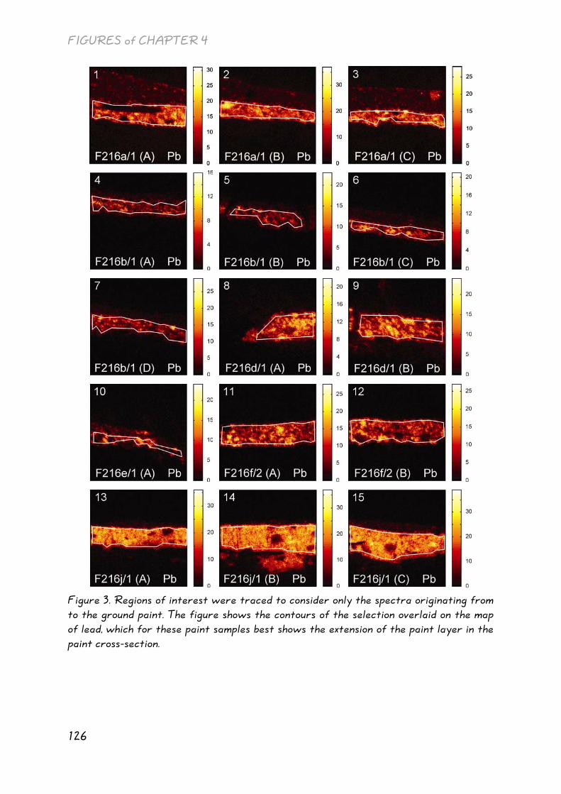
FIGURES of CHAPTER 4
126
Figure 3. Regions of interest were traced to consider only the spectra originating from to the ground paint. The figure shows the contours of the selection overlaid on the map of lead, which for these paint samples best shows the extension of the paint layer in the paint cross-section.

FIGURES of CHAPTER 4
127
Figure 4. Regions of interest were traced to consider only the spectra originating from to the ground paint. The figure shows the contours of the selection overlaid on the map of lead, which for these paint samples best shows the extension of the paint layer in the paint cross-section.
Figure 5. Plots of principal component loadings obtained after principal component analysis performed on the ensemble of all acquisitions.

FIGURES of CHAPTER 4
128
Figure 6. Principal component score plots of the first principal component. The colour scale is chosen to provide a visual distinction between the positive (in warm tints) and negative components (in cold tints) in the loadings.

FIGURES of CHAPTER 4
129
Figure 7. Principal component score plots of the first principal component. The colour scale is chosen to provide a visual distinction between the positive (in warm tints) and negative components (in cold tints) in the loadings.

FIGURES of CHAPTER 4
130
Figure 8. Principal component score plots of the third principal component. The colour scale is chosen to provide a visual distinction between the positive (in warm tints) and negative components (in cold tints) in the loadings.

FIGURES of CHAPTER 4
131
Figure 9. Principal component score plots of the third principal component. The colour scale is chosen to provide a visual distinction between the positive (in warm tints) and negative components (in cold tints) in the loadings.
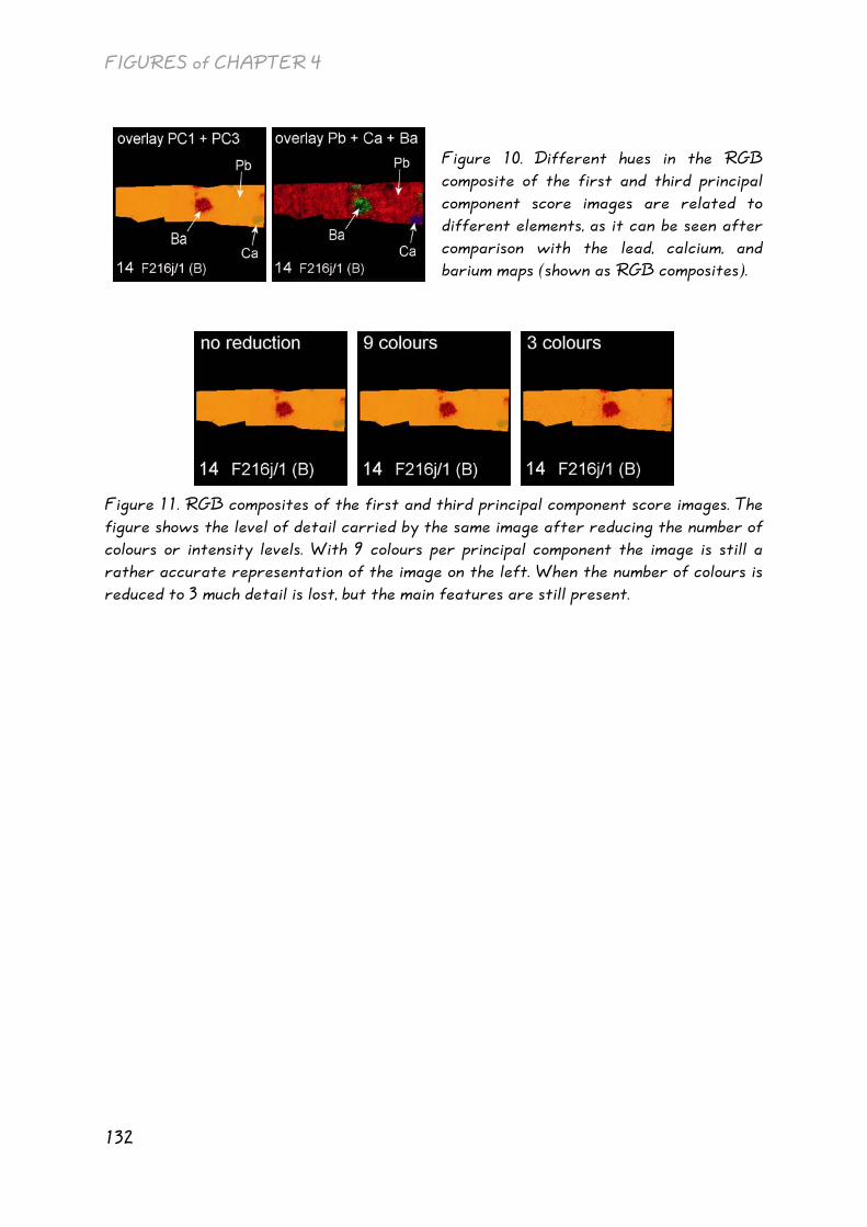
FIGURES of CHAPTER 4
132
Figure 10. Different hues in the RGB composite of the first and third principal component score images are related to different elements, as it can be seen after comparison with the lead, calcium, and barium maps (shown as RGB composites).
Figure 11. RGB composites of the first and third principal component score images. The figure shows the level of detail carried by the same image after reducing the number of colours or intensity levels. With 9 colours per principal component the image is still a rather accurate representation of the image on the left. When the number of colours is reduced to 3 much detail is lost, but the main features are still present.

FIGURES of CHAPTER 4
133
Figure 12. RGB composites of the first and third principal component score images. In these images the number of intensity levels per principal component was reduced to 9.

FIGURES of CHAPTER 4
134
Figure 13. RGB composites of the first and third principal component score images.In these images the number of intensity levels per principal component was reduced to 9.
Figure 14. Examples of histogram extracted from the RGB composites of score images, with 3 and 9 colours per channel. The correspondence between colour shades and elemental composition is shown.

FIGURES of CHAPTER 4
135
Figure 15. Histograms of RGB composites of score images for all acquisitions (3 colours per channel).

FIGURES of CHAPTER 4
136
Figure 16. Histograms of RGB composites of score images for all acquisitions (9 colours per channel).

FIGURES of CHAPTER 4
137
Figure 17. Dendrograms obtained after cluster analysis made on the histograms (top: 3 colours per channel, bottom: 9 colours per channel). Histograms representative of the classes identified are displayed below the dendrogram.

FIGURES of CHAPTER 4
138
3 colours
9 colours
Cluster number
acquisition
number acquisition
sample code (area) acquisition
number acquisition
sample code (area)
1
2, 3 9 11, 12 21 22
F216a/1 (B, C) F216d/1 (B) F216f/2 F296/2 (B) F369/1 (A - white)
2, 3 9 11, 12 21 22, 23, 25
F216a/1 (B, C) F216d/1 (B) F216f/2 F296/2 (B) F369/1 (A, C)
2
1 4, 5, 6, 7 23, 24, 25
F216a/1 (A) F216b/1 F369/1 (A - beige, B, C)
1 4, 5, 6, 7 24
F216a/1 (A) F216b/1 F369/1 (B)
3
8 13, 14, 15 16, 17, 18
F216d/1 (A) F216j/1 F267/2
8 13, 14, 15 16, 17, 18
F216d/1 (A) F216j/1 F267/2
4
10 19 20
F216e/1 F294/1 F296/2 (A)
10 19 20
F216e/1 F294/1 F296/2 (A)
Table 1. Result of cluster analysis made on principal component scores image stacks (PC1 and PC3). In the analysis 3 and 9 intensity (or colour) levels per principal component channel were considered. The table lists the sample acquisitions belonging to each of the classes identified by cluster analysis. The numbering and coding of individual acquisitions correspond to those used in the figures.
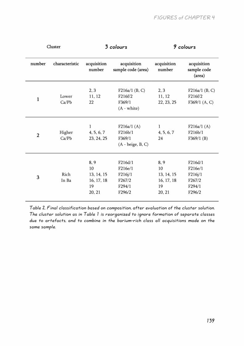
FIGURES of CHAPTER 4
139
Cluster
3 colours
9 colours
number characteristic acquisition number
acquisition sample code (area)
acquisition number
acquisition sample code
(area)
1 Lower Ca/Pb
2, 3 11, 12 22
F216a/1 (B, C) F216f/2 F369/1 (A - white)
2, 3 11, 12 22, 23, 25
F216a/1 (B, C) F216f/2 F369/1 (A, C)
2 Higher Ca/Pb
1 4, 5, 6, 7 23, 24, 25
F216a/1 (A) F216b/1 F369/1 (A - beige, B, C)
1 4, 5, 6, 7 24
F216a/1 (A) F216b/1 F369/1 (B)
3 Rich In Ba
8, 9 10 13, 14, 15 16, 17, 18 19 20, 21
F216d/1 F216e/1 F216j/1 F267/2 F294/1 F296/2
8, 9 10 13, 14, 15 16, 17, 18 19 20, 21
F216d/1 F216e/1 F216j/1 F267/2 F294/1 F296/2
Table 2. Final classification based on composition, after evaluation of the cluster solution. The cluster solution as in Table 1 is reorganized to ignore formation of separate classes due to artefacts, and to combine in the barium-rich class all acquisitions made on the same sample.

FIGURES of CHAPTER 4
140
Qualitative classification
Quantitative classification
Sample
code colour composition
F216a/1 * 1 1 1 / 2 *
F216b/1 1 2 2
F216d/1 2a 1 3
F216e/1 2a 2 3
F216f/2 2a 1 1
F216j/1 2a 1 3
F267/2 2b 2 3
F294/1 2b 2 3
F296/2 2b 2 3
F369/1 extra 1 1 / 2
* contains menilite
Table 3. Summary of the classifications of the ground paints. The qualitative classification was made by examination of support, paint surface, and paint cross-sections. The quantitative classification was made separately on the basis of colour and composition of the paint at the microscopic level. The numbers correspond to classes as follows (for the same sample multiple numbers are shown when different acquisitions are assigned to different classes). Qualitative classification: 1 = white grounds, 2a = grey grounds, batch A, 2b = grey grounds, batch B. Colour: 1 = light-coloured grounds, 2 = grey grounds. Composition: 1 = lower Ca/Pb, 2 = higher Ca/Pb, 3 = Ba rich.

141
Quantitative analysis of composition
of ground paints in paint cross-sections
Recipe for chocolate sauce. Ingredients:
10 ounces bittersweet or semisweet chocolate, chopped into small pieces 1/3 + 3/4 cup milk, half-and-half, or heavy cream,
or 1/2 to 3/4 cup milk plus 2 tablespoons butter.
...The beauty of this recipe is that you can tailor it to your own taste and the type of chocolate you are using.
...For an even more intense chocolate experience, choose a bittersweet chocolate labeled anywhere between 66 to 72 percent.
Alice Medrich, ‘Chocolate Holidays’

CHAPTER 4
142
4.1 INTRODUCTION In the previous Chapter we made a quantitative classification of ground paints on the basis of their colour. The colour information was extracted at the microscopic level from light-microscopic images of the paint cross-sections. The method involved extraction of the colour distribution (histogram) within a region of interest for all images, the calculation of an index of similarity between the distributions, and classification by hierarchical clustering techniques. The method proved to be successful and efficient and showed potential. However it appeared that, for our case study, the classification would benefit from additional information, because the colours have a direct relationship with the material properties of the constituent materials in the grounds. Both the need for integrating additional information and the efficacy of the method have encouraged to expand the method SIMS data, discussed in Chapter 2, acquired on the same samples. SIMS was preferred to SEM-EDX because of its surface sensitivity and higher lateral resolution. In fact SEM-EDX used at conventional beam energies (> 10 keV) is not surface sensitive because of the large interaction volume of probing electrons inside the sample [Goldstein et al. 2003]. The approach that we used for the colour-based comparison does not make assumptions on the type of data being compared, and can be extended to work on different types of spectral imaging data. Obviously some modifications are necessary in order to adapt the methodology to a specific type of dataset and to address both

CHAPTER 4
143
conceptual and practical issues in its application. A primary issue is to handle the enormous amount of information contained in imaging spectral data, and to provide concise and easily interpretable in output. The present Chapter is structured as follows. First the methodology is described, illustrating how different issues are addressed. In a second part we will discuss the application to our case study. 4.2 MATERIALS AND METHODS
4.2.1 SAMPLES AND ANALYTICAL TECHNIQUES The SIMS data analysed in this Chapter are the same ones as in Chapter 2. A total of 25 acquisitions made on 10 paint samples are analysed. In order to make a meaningful comparison of the images, SIMS data were acquired under the same analytical conditions by rastering a 100 µm x 100 µm area with a pulsed 15 kV primary ion beam from an In115 liquid metal ion tip, non-bunched with a pulse width of 20 ns, 600 pA current, spot size of ~120 nm, and with charge compensation. For more details on sample preparation, data acquisition conditions, and image extraction, the reader is referred to Chapter 2.
4.2.2 DATA PROCESSING The data analysis was performed with software, developed in Matlab environment (version 6.5, The Mathworks, Inc.) by Beatrice Marino at the FOM-AMOLF Institute in Amsterdam. The software developed for the application presented here is based on and constitutes a large extension of the software package GAIM developed earlier at AMOLF by Jaap van der Weerd. The analysis was run on an Acer TravelMate 800 laptop computer with an Intel Centrino 1.6 GHz, 1 GB Level 2 cache processor and 768 MB RAM, Windows XP OS, with reasonable computational effort.

CHAPTER 4
144
4.3 METHODOLOGY OF COMPARISON OF THE MATERIAL COMPOSITION
4.3.1 GENERAL CONCEPTS 4.3.1.1 Analogy between colour images and imaging mass-spectrometric data The general idea in our method of comparing imaging compositional information is the same as used to compare colours in digital images. A comparison between these two types of data will highlight the similarities that allow the extension of the method to imaging-SIMS data. A colour RGB image contains spatially arranged colour information in three colour channels (red, green, and blue). Likewise, an imaging SIMS dataset contains spatially arranged compositional information in N mass channels, where N is a variable number that depends on mass range and resolution. In this sense, SIMS datasets can be considered an extension of RGB images and are handled similarly. All colours in a colour image can be reproduced from the combination of three colour channels, which represent primary colours. Each colour channel is an image representing the intensity of the light reflected off points on the sample surface, for the corresponding primary colour. A number quantifies this amount in each pixel or point in the digital image. Therefore, pixels in the image represent colours at different sample locations, by using triplets of numbers for each pixel. The maximum number of colours that can be represented depends on the number of different intensity values that are considered for the colour channels. One can summarize the distribution of colours in the image, by counting for each colour the number of pixels that represent it, discarding the spatial information. Basically, relative intensities in the histogram represent the relative amounts of different colours in the image. The same argument can be developed for imaging mass-spectral datasets as those obtained by SIMS. An imaging SIMS dataset represents compositions in a similar way as colour images represent colour. Therefore in this Chapter we will refer to ‘mass channels’, ‘compositions’, and ‘compositional histograms’ instead of ‘colour channels’, ‘colours’, and ‘colour histograms’. In a SIMS dataset the ‘mass channels’ represent individual elements or ions, and their combination represents a particular composition. Each mass channel is an image or map representing the number of ions of that mass expelled by the sample surface reaching the detector. A number quantifies this amount in each point in the map. Therefore, pixels represent compositions at different sample locations, by using

CHAPTER 4
145
N numbers for each point. One can summarize the ‘distribution of compositions’ in the dataset, by counting for each composition the number of points that represent it, discarding the spatial information. Basically, relative intensities in the histogram represent the relative amounts of different compositions in the image. 4.3.1.2 Adapting the method of colour comparison to imaging SIMS data The argumentation given above shows that imaging SIMS data can be compared quantitatively by adopting the same processing method used with colour images. As in the method for colour comparison, there are four main steps, which consist in reduction and extraction of data, histogram extraction, comparison, and classification. The idea is to extract ‘compositional histograms’ for all ground paints from the SIMS data, to compare them for generating similarity indices, and to use these indices to identify classes of similar grounds. The application of the method to SIMS datasets requires a number of modifications in order to adapt it to the type of dataset and to address conceptual and practical issues. The modifications occur mainly in the first step, and consist of a number of data reduction and extraction sub-steps. The individual data processing steps are discussed in detail in the following Sections; the first step will be illustrated most extensively, as the other ones were already presented in Chapter 3. A scheme of the method illustrating the processing steps is shown in Figure 1 (the figures of this Chapter can be found at p. 124-140).
4.3.2 FIRST STEP: DATA REDUCTION AND FEATURE EXTRACTION The need for data reduction and feature extraction arises from the huge amount of data contained in imaging SIMS datasets, whose dimensionality is generally much larger than colour images. In fact, each pixel in a SIMS image contains a full mass-spectrum, which may contain thousands of peaks [Tyler 2001]. There is a fundamental distinction between data reduction and feature extraction. The aim of data reduction is to reduce the size of a dataset, mainly for practical purposes as for example to reduce the computational effort in processing and analysis of data when these are large. Feature extraction is the process of identifying, selecting and extracting relevant features from the dataset, discarding irrelevant features. Relevant features are those that provide a good representation of a sample with respect to the aim of the study. Irrelevant features include noise as well as other characteristics that are not useful for the analysis. Feature extraction, and possibly also data reduction, simplifies the representation of data, makes the data analysis process more efficient, and facilitates the interpretation of results.

CHAPTER 4
146
The first processing step is structured as follows. Data reduction is performed at first during import of the raw data, by downsampling the mass spectra and reducing the mass range to a range of interest. Then relevant features are extracted, and regions of interest are traced on the distribution elemental maps. Data are further reduced by downsampling of the intensity levels. Finally we apply principal component analysis, which plays the double role of data compression and of pattern recognition tool, by identifying relevant components that characterize the specific set of samples under analysis. 4.3.2.1 Importing datasets The first data reduction occurs when raw data are imported into Matlab. In the raw data, after each primary ion beam pulse, counts for all ion species are recorded sequentially as ions reach the detector. The import process reorganises data for subsequent processing in a three-dimensional array, where each point corresponding to a location on the sample surface contains a full mass spectrum. The array can also be considered as a stack of images, one image for each ion mass peak. The number of peaks can be extremely large depending on mass range and mass resolution. In the import process mass range and mass resolution can be reduced to obtain data reduction. The mass range is simply chosen in order to include all the masses of interest. Mass resolution determines the extent to which mass peaks are binned together, and its choice is a trade-off between data size reduction and preservation of quality. A high mass resolution is necessary to resolve adjacent peaks of different ion species. For example inorganic ions peaks are accompanied by shoulder organic peaks, which for paint cross-section samples can originate from the polymer used for embedding. A low mass resolution results in high compression of mass spectra, with consequent increase of computational efficiency in both the import process and the subsequent data processing steps, but care must be taken in order to avoid merging of adjacent peaks due to decreased resolution. Therefore, an appropriate value for the mass resolution is high enough so that peaks that are partially overlapping are not being merged in a single peak in the import process. Since selecting only a relatively small number of features leads to a considerable reduction in data dimensionality, the limitations in the choice of mass resolution in importing the data is loosened. Working at a higher mass resolution, allows extracting peaks of interest while resolving them from shoulder peaks with better accuracy.

CHAPTER 4
147
However, the choice of the mass resolution is not critical in the method that we adopted, as further data reduction will be obtained in subsequent steps. In fact the analysis is performed on distribution maps of selected ion species, and which are generated by integration within a range around the nominal mass. 4.3.2.2 Feature selection Data pretreatment often involves selection of features. This may be done either by removing unwanted peaks, or by extracting only the peaks of interest. The choice of the method to use depends on the particular application, and is made by taking into account a number of practical considerations [Wagner et al. 2004]. The ground paints under study have a quite simple composition, characterized by a few elements (see Chapter 2). Feature extraction therefore simultaneously leads to a considerable further data reduction and to the elimination of a large fraction of chemical noise. Distribution maps of characteristic elements are generated by manual selection of a mass range around the nominal masses. Appropriate choice of mass resolution during the import process allows performing the selection with accurate precision, in order to exclude background and shoulder peaks. In our case a mass resolution of 0.01 amu was considered sufficient to provide resolution of adjacent peaks with reasonable import process duration. The distribution map is obtained by summing the intensities within the selected mass range at each position in the map. The maps are arranged in an image stack for each individual sample acquisition, and saved in a separate data file. Descriptions and information on the distribution maps (m/z value, element name, position in the image stack) are also included for reference in the form of a list. The procedure for storing images and related information was standardized in order to have a consistent arrangement in the data files for all acquisitions. To this end, the user is first required to create a list of a fixed number of entries, and to enter information such as mass and a description for each slot. The distribution maps can then be stored according to the preset order. The list can be reused for the other datasets to be compared. 4.3.2.3 Selection of regions of interest Regions of interest can be hand selected. All pixels in the maps outside the selection are set to zero.

CHAPTER 4
148
4.3.2.4 Principal component analysis The main difference of the present method with respect to that of colour comparison in Chapter 3 is the application of Principal Component Analysis.
PCA as a data compression tool Principal Component Analysis (PCA) is the most commonly used method of multivariate analysis, which is a collection of unsupervised statistical methods that provide a concise representation of data. Multivariate analysis techniques are therefore widely used to reduce the dimensionality of datasets with a large number of variables, such as spectral and multispectral datasets, in order to facilitate their interpretation [Geladi and Grahn 1996, Sharma 1996]. They are especially useful in spectral imaging applications, where data represent a huge assembly of information, and it consequently found increasing interest in more recent years [Geladi and Grahn 1996, Graham et al. 2005, Tyler 2001, Tyler 2005, Wagner et al. 2004, Wickes et al. 2003]. In our case, PCA is extremely useful to reduce the dataset to a size of the same order of that used for comparing colour images, making feasible the comparison of imaging mass-spectrometric data. This simplification is achieved in a quantitatively rigorous fashion. The underlying concept is to identify a small set of new variables that effectively describe the data with minimal loss of information, by finding relationships between variables and between spectra [Geladi and Grahn 1996, Matlab documentation, Sharma 1996]. In a dataset variables arising from the same chemical or physical principle vary together. For example, in a mass-spectral dataset of a system consisting of two materials, ion yields of ions emitted from the same material are correlated, while yields of ions originating from different materials are anti-correlated. This redundancy of information can be used to simplify the dataset. Principal component analysis captures these correlations in new variables, called principal components. These new variables, which represent patterns in the dataset, are uncorrelated and therefore do not contain redundant information1.
1 An intuitive example illustrating this concept is that of cakes. Cakes can be made with a variety of ingredients (e.g. flour, eggs, sugar, butter, chocolate, fruit, liquor, cream, etc). A cake can be described in terms of its ingredients and the amounts used. This is the equivalent of a mass-spectrum. With principal components we can find patterns in the compositions of a set of cakes, and describe them in terms of standard recipes, which represent types of cakes (e.g. chocolate cake, fruit cake, etc.). The recipes identified with PCA are those that best represent the particular set of cakes analysed, and not all the recipes that can be made with the ingredients considered. The recipes

CHAPTER 4
149
Formulation of PCA Principal component analysis generates three outputs, the scores, the principal component loadings, and the eigenvalues. The scores are the dataset expressed in terms of principal components. The loadings express the relationship between the old variables (masses) and the new variables (the principal components). They give an indication of the extent to which the old variables influence the formation of principal components, assisting in the interpretation of the scores. Loadings group peaks with strong covariance, which are likely to arise due to the same chemical or physical phenomenon. The eigenvalues are scalars associated to the principal components, which, normalized to one, express the percent of variance carried by each principal component. Mathematically, principal components are derived to represent the directions of greatest variations in the dataset. These directions are identified by the loadings, which are calculated as the eigenvectors of the data covariance matrix. Once the loadings are known, we can calculate the data represented in terms of the new variables, the scores, as: S = D L (1) where D is the original dataset, L is an array whose columns are the loading vectors, and S are the scores. In this expression, the dataset is rearranged from a three-dimensional into a two-dimensional array, in which each row is a spectrum. The spectra of individual pixels are therefore treated as separate samples. The scores can be reorganized into a stack of images, each image corresponding to a principal component. Therefore, together with the loadings, the scores provide an excellent means of evaluating the results of PCA. Principal components are sorted by decreasing eigenvalues, so that the first principal components are those containing the information that is most relevant to describe the particular dataset under analysis.
found are standard, but in practice they can be varied in the preparation of a cake. Therefore in general no cake can be entirely represented by a single recipe, and an exact description involves multiple recipes. In a simplified representation, the recipe that best fits a particular cake will be used to describe the type of cake.
CHAPTER 4
150
PCA as a tool for data comparison and classification Usually, most of the variance in the data is carried by only a few principal components. This is especially useful in applications in which multiple datasets are being compared, where principal component analysis performed on the ensemble of all the datasets would capture the features that account for differences between the individual datasets. These features can then be used to attempt the identification of groups of samples that share similar characteristics, and the discrimination between these groups. In addition, PCA tends to separate characteristic features, on the basis of their correlation, into separate principal components. In conclusion, selection of only few principal components results simultaneously in efficient data reduction (which is substantial if the number of the original variables is large), improved performance of subsequent analysis methods, and simplification of the interpretation of results. Since the decision on the number of principal components to retain depends on the amount of information that is considered relevant, the eigenvalues are used as a criterion. One of the most used criteria is to plot the eigenvalues and to look for an elbow. After PCA, compositions are no longer represented by proportions of elements but by principal components, which are combinations of elements. Following again the parallel with colour images, from this point forward we will consider ‘principal component channels’ instead of ‘mass channels’. We will retain the same expressions of ‘composition’ and ‘composition histogram’, as analogous to ‘colour’ and ‘colour histogram’, which we defined for mass-spectral data before PCA. 4.3.2.5 Reduction of number of intensity levels In order to reduce the computational load in the extraction of ‘compositional histograms’, it is necessary to decrease the number of intensity values. In a colour image this process corresponds to reducing the number of different colours to a smaller set, by approximating colours in the image to the most similar in the set. In mass-spectrometric data, ‘reducing the number of compositions’ translates in considering fewer different combinations of material proportions. Following this analogy, we will equivalently refer to the intensity levels in mass-spectrometric data as colours. This number is chosen to simplify the data to capture only the information essential for discriminating between samples. It can be determined by evaluating the quality of the reduced score images (and of their RGB composites, described below, if the

CHAPTER 4
151
number of principal components considered is 3 or less), histograms, and classification. The reduced score images provide an immediate insight into the degree of accurateness with which they represent the original scores. On the other hand, the histograms show whether the information retained allows discrimination between samples. It should be noticed that an overly accurate representation does not necessarily improve or lead to the identification of classes of similarities. In fact, small within-sample intensity fluctuations might not assist in the classification process by concealing between-sample differences. In conclusion, a convenient choice of the number of intensity levels will lead to a classification that is congruent with similarities and differences between samples, and of simple interpretation at the same time. 4.3.2.6 Stacks and RGB composites of score images The score images obtained after PCA can be combined for each acquisition dataset into a stack of images. When three or fewer principal components are considered, the score images can be conveniently visualized as RGB images. In the RGB composite, each principal component score image is represented in one of the primary colours. This representation is extremely useful for evaluation of the output of PCA in view of the subsequent classification. The principle of making RGB composites is illustrated in Figure 2. RGB composites show through colour or tint differences how classes of pixels are formed from the combination of score images. The association between colours and principal components allows the identification of those components that are most representative for each class. Colour classes can then be related to the sample chemistries through examination of the loadings. In this way false-colour composites indicate how different chemistries are discriminated depending on which principal components are considered. The chemistry classes are captured by the histograms extracted from the stacks of score images. The last statement is valid also when considering more than three principal components, although it is not possible to make false-colour composites.
4.3.3 SECOND STEP: HISTOGRAM EXTRACTION From this point on, data processing is performed exactly as in the comparison of colour images. For the mathematical expressions the reader is referred to Chapter 3. Histograms are extracted by counting the number of pixels representing each ‘composition’. The mathematical representation of this operation is the same used

CHAPTER 4
152
for colour images, the only difference being that there are no restrictions on the number of ‘principal components channels’.
4.3.4 THIRD STEP: HISTOGRAM COMPARISON In the previous Chapter colour histograms were compared by using a weighted quadratic distance, where the weights account for the similarity between individual colours. Although originally intended for comparing colours in images, this metric is suitable for measuring the similarity of compositions as well. In fact, it is both intuitive and reasonable to consider as similar spectra that exhibit small variations in relative amounts of the same constituents. With colours, shades of the same hue (for instance, red) are more similar with each other relatively to a different hue (for instance, blue). Similar shades or large colour differences are due respectively to small or large variations in the light reflected off the sample surface, which in turn are represented in a colour image by small or large numerical differences. Similarly, variations in compositions correspond to consistently small or large differences in the proportions of constituent elements, which are reflected by relative ion yields in the mass spectra.
4.3.5 CLASSIFICATION BY HIERARCHICAL CLUSTER ANALYSIS The classification is performed by means of hierarchical cluster analysis methods. The concepts of cluster analysis and the mathematical expressions were already given in Chapter 3.

CHAPTER 4
153
4.4 CASE STUDY: GROUNDS IN PAINTINGS BY VAN GOGH In the present Section we discuss the application of the method illustrated in the previous Section to imaging SIMS data of selected grounds in paintings by Van Gogh. The data considered here are the same that were discussed qualitatively in Chapter 2.
4.4.1 APPLICATION TO THE DATASETS The datasets of positive mode spectra were first imported into Matlab with a mass range 0-250 m/z and downsampled to a mass resolution of 0.01 amu and saved in a new data file. The mass range is sufficiently large to include all the characteristic elements that were identified in Chapter 2, namely aluminium (m/z 27), calcium (m/z 40), iron (m/z 56), strontium (m/z 88), barium (m/z 138), and lead (m/z 208). We excluded magnesium (m/z 24) from the analysis because, although characteristic of the discriminating feature of menilite, under SIMS it cannot be distinguished from the overlapping contributions from silicon carbide particles of the polishing paper. In the present study we do not discriminate between calcium carbonate and gypsum. In order to discriminate between calcium carbonate (CaCO3) and gypsum (CaSO4), information on calcium and sulphur, acquired at different ion modes (respectively, positive and negative), should be combined after image registration. However this is beyond the scope of the current work, and we will restrict the analysis to calcium maps alone2. The mass resolution is sufficiently high to resolve the peaks of interest from shoulder organic peaks and to have reasonable processing time and data file size.
2 SEM-EDX in principle is also able to provide sulphur information, unfortunately overlapping in the x-ray spectrum of the sulphur K line with lead M line, makes it unsuitable for the analysis of paint samples containing also lead-based materials, unless a deconvolution routine is available in the analysis software. An interesting tool that might be considered in future works for the identification of different phases is Electron BackScattering Diffraction (EBSD) [Goldstein et al. 2003]. This technique allows distinguishing different chemical phases, even of similar or exact compositions, from the crystallographic information contained in diffraction patterns. EBSD is a surface-sensitive technique, and it does not suffer the same disadvantages of SEM-EDX caused by large interaction volumes. EBSD measurements require an extremely flat sample surface, which can be obtained by ion milling.

CHAPTER 4
154
Regions of interest were traced in each sample acquisition, in order to exclude from the analysis spectra collected from sample locations outside the ground paint area. The regions were hand traced on the distribution map of lead (Figures 3-4), which provides the best distinction between the ground paint layer and the upper paint layer where present, and applied to all maps in the image stack. Prior to principal component analysis, all acquisitions were combined as a mosaic in a single image stack, and the data were normalized. Spectra were normalized individually to their total intensity, in order to eliminate fluctuations in the experimental conditions that do not relate to the sample chemistry [Graham et al. 2005, Wagner et al. 2004]. In our case, an apparently appropriate choice would consist of normalizing all spectra in a individual sample dataset to the value of the highest peak in the dataset, in order to preserve local intensity variations. PCA performed on images normalized in this way indeed produced score images with greater compositional differences detail. However this resulted in classifications where local concentration variations dominated between-sample compositional differences. Instead, individual normalization of each spectrum to its total intensity, despite producing images with lower compositional contrast, was found to lead to a classification that is more informative of between-sample differences.
4.4.2 ANALYSIS OF PCA OUTPUT The principal component loadings are plotted in Figure 5. The relative eigenvalues indicate that the first three principal components account for 99 % of the variation contained in the original dataset. However, as it will be explained below, only the first and the third principal component score images were used for the subsequent analysis. The principal component score images for all acquisitions are shown in Figures 6-9. The colour map used for displaying the scores was defined in order to distinguish points with positive and negative loading components. Positive components are represented in warm colours, with shades from red to yellow corresponding to low to high values. Negative components are represented in cool colours, with shades from blue to green corresponding to absolute values from low to high. Areas lying outside the regions of interest and points with no components on the loading are represented in black. With this colour scheme, points whose elemental compositions are correlated are represented with colours of the same warmness, and those anti-correlated with colours of opposite warmness.

CHAPTER 4
155
4.4.2.1 Loadings and score images The first principal component loading is dominated by lead, followed by calcium; the contribution of calcium is relatively low, and closer to those from other elements. Correspondingly, the score images show compositional contrast between lead (in yellow) and the other elements, most noticeably calcium and barium (in red). The score images of the first principal component (Figures 6-7) therefore enable to distinguish samples on the basis of relative amounts of lead to other materials. The loading plot of the second principal component shows a high positive component value for calcium, a low negative component for lead, and a low positive component for the remaining elements. The score images (not shown) therefore differentiate between these three groups of elements (respectively in yellow, blue, and red). Barium is the characteristic component of the third principal component loading. The corresponding score images highlight barium (displayed in Figures 8-9 in shades of green and blue depending on the concentrations in the sample), against all the other elements (in red). 4.4.2.2 RGB composites of score images Since we are considering only two principal components, RGB composites of the score images can be made to assist in the analysis. For the samples under investigation, the RGB composites show that the combination of the first (red channel) and third (green channel) principal component score images provides a good discrimination of different compositions. An example is illustrated in Figure 10. Comparison of an RGB composite of the score images with the maps of lead, calcium, and barium combined without applying PCA shows that the distinction is essentially based on lead, calcium, and barium containing materials. As mentioned earlier, the second principal component was excluded from the analysis, because the variation it carries was not found to be informative of between-sample differences. The inclusion of the second principal component would introduce an additional colour class, which corresponds to areas of comparable concentrations of calcium and lead rather than to a separate chemical feature. While being nevertheless characteristic of the sample compositions, this class was found to dominate other, relevant features in the comparison, leading to complex sample classifications that were hard to interpret.

CHAPTER 4
156
4.4.2.3 Choice of number of intensity levels Before extracting the histograms, the number of different intensity levels was reduced, and consequently the number of different colours in the RGB composites. The quality of the RGB composites of score images in terms of preservation of relevant features, assessed by visual inspection, is preserved even at very low number of intensity levels (down to 5 per channel). In Figure 11 images of the same RGB composite before colour reduction, with 9 colours per channel, and with 3 colours per channel are compared. A sufficiently high number of colours preserves small-scale variations occurring along the boundaries between areas of different elemental compositions, or are due to inhomogeneity in material concentrations within individual sample areas or particles. At 3 colours per channel the level of approximation is still strong. The main compositional features are still preserved, and are simplified after elimination of small-scale variations. In general we have observed that there are no significant differences in the cluster solution for number of colours per channel larger than 5. Therefore in the following discussion we will consider only the two cases of 3 and 9 colours per channel, examining the differences in the cluster solutions, the factors affecting the results, and in their interpretation. Figures 12-13 show the RGB composites for all acquisitions with 9 colours per channel.
4.4.3 CORRESPONDENCE BETWEEN COLOURS IN RGB COMPOSITES AND SAMPLE COMPOSITION
The chemical characteristics of the clusters can be identified by examining and comparing the RGB composites of score images and their histograms. Since we considered only two principal components, the histograms can be conveniently plotted as in the examples of Figure 14. The figures also indicate the correspondence between colours and elemental composition. Hues of orange, red and green mainly represent, respectively, lead, barium, and calcium. Depending also on the combination of the score images and on the level of approximation, colour shades are related to variations in ion yields related to differences in concentrations, surface irregularities, mixed compositions, and noise. Mixed compositions in the dataset may arise from different materials that are mixed as fine particles, or as fine particles filling surface irregularities in larger particles, and that are not spatially resolved. All the possible colours that can be obtained with the chosen number of intensity levels per channel are shown in the histogram plots on the horizontal plane. Vertical

CHAPTER 4
157
bars above the plane represent the frequency with which colours occur that are present in the image. Figures 15-16 show the histograms corresponding to images containing respectively 3 and 9 colours per channel, for all acquisitions. Since the peak corresponding to lead is consistently and significantly dominant, the vertical axis was downscaled for better visualization of the other peaks. In the adopted representation, spatial closeness of colours on the plane corresponds to similarity of the compositions that they represent. This allows an immediate and effective perception and understanding of the characteristics of individual histograms and of the corresponding chemical information, as well as of the similarities and differences that lead to the formation of clusters, and leads to the identification of classes. Intermediate colour shades originate from small-scale variations of ion yields and mixtures of signals from different elements.
4.4.4 ANALYSIS OF THE CLUSTER SOLUTION Similarly to the case of colour comparison, single-linkage, complete-linkage, and average-linkage produced similar results, with the complete-linkage method providing the best clustering. Figure 17 (p. 159) illustrates the dendrograms obtained after cluster analysis with complete-linkage. The dendrograms suggest that there are four clusters or classes, to which we refer as 1, 2, 3, and 4. Four histograms that were chosen as representative of the four classes identified by the clusters are depicted below the dendrograms. Table 1 lists the individual sample acquisitions belonging to each class. 4.4.4.1 Case of 3 colours per channel We first examine the results obtained with 3 colours per channel. The clustering method is able to distinguish between samples containing barium (classes 3 and 4) from those containing no or negligible amounts of barium (classes 1 and 2). Finer differences in composition are captured by individual classes. The difference between classes 1 and 2 consists in the relative concentrations of calcium to lead. The distinction between classes 3 and 4 is related to different relative heights of peaks associated to barium. Inspection of the RGB composites show that, in samples belonging to class 3, the barium particles (in red) are surrounded by an orangey-red ‘halo’ (corresponding to the tall peak on the left side of the colour plane in Figure 14). In the unprocessed barium maps (see Chapter 2), this ‘halo’ consists of

CHAPTER 4
158
sparsely- distributed pixels surrounding a dense ‘core’ of pixels. BSE images (see Appendix B at the end of this Thesis) of the areas reveal that the region corresponding to the ‘halo’ does not lie within barium particles. The ‘halo’ is rather an artefact resulting from a noise-rich area, which in the process of colour reduction is converted into a homogeneously coloured area. Therefore classes 3 and 4 should be considered as a single class. It can be noticed that different acquisitions made on the same sample may be classified differently depending on sample inhomogeneity. For example acquisition F296/2 (A), which shows a large barium particle, is classified in cluster 4, while acquisition F296/2 (B) does not contain barium and is classified in cluster 1. We also observe that the role of lead in the classification is relative to other elements, because of its consistently dominant fraction in the compositions. 4.4.4.2 Case of 9 colours per channel The histograms extracted from images with 9 colours per channel are more structured. Despite the apparent complexity, the increase in the level of detail, which is also visible from the redistribution of histogram peaks into multiple colour shades, emphasizes the differences between classes. The increase in number of colour shades is particularly pronounced for the hue related to barium, enhancing small variations in concentrations. The ‘haloes’ observed above in the RGB composites with 3 colours per channel can now be identified as noise pixels. The cluster solution observed above essentially does not change when 9 colours per channel are considered. The same considerations made in the previous case hold also in this case. 4.3.2.2 Additional and final considerations The considerations made above lead to the classification presented in Table 2. The cluster solution as in Table 1 is reorganized to ignore formation of separate classes due to artefacts, and to combine all acquisitions in the barium-rich class made on the same sample. The cluster solutions observed in the two cases are in agreement with each other, the identification of these classes being essentially unaffected by the number of intensity levels considered. The differences in the way classes are joined in the dendrograms should not be considered as inconsistencies. In fact the cluster solution is defined only as the clusters identified by cutting the dendrogram at a certain
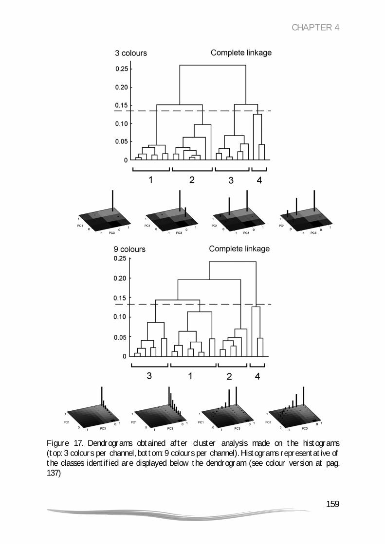
CHAPTER 4
159
Figure 17. Dendrograms obtained after cluster analysis made on the histograms (top: 3 colours per channel, bottom: 9 colours per channel). Histograms representative of the classes identified are displayed below the dendrogram (see colour version at pag. 137)
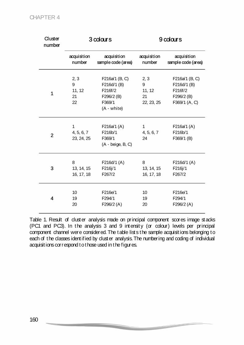
CHAPTER 4
160
3 colours
9 colours
Cluster number
acquisition
number acquisition
sample code (area) acquisition
number acquisition
sample code (area)
1
2, 3 9 11, 12 21 22
F216a/1 (B, C) F216d/1 (B) F216f/2 F296/2 (B) F369/1 (A - white)
2, 3 9 11, 12 21 22, 23, 25
F216a/1 (B, C) F216d/1 (B) F216f/2 F296/2 (B) F369/1 (A, C)
2
1 4, 5, 6, 7 23, 24, 25
F216a/1 (A) F216b/1 F369/1 (A - beige, B, C)
1 4, 5, 6, 7 24
F216a/1 (A) F216b/1 F369/1 (B)
3
8 13, 14, 15 16, 17, 18
F216d/1 (A) F216j/1 F267/2
8 13, 14, 15 16, 17, 18
F216d/1 (A) F216j/1 F267/2
4
10 19 20
F216e/1 F294/1 F296/2 (A)
10 19 20
F216e/1 F294/1 F296/2 (A)
Table 1. Result of cluster analysis made on principal component scores image stacks (PC1 and PC3). In the analysis 3 and 9 intensity (or colour) levels per principal component channel were considered. The table lists the sample acquisitions belonging to each of the classes identified by cluster analysis. The numbering and coding of individual acquisitions correspond to those used in the figures.

CHAPTER 4
161
Cluster
3 colours
9 colours
number characteristic acquisition number
acquisition sample code (area)
acquisition number
acquisition sample code
(area)
1 Lower Ca/Pb
2, 3 11, 12 22
F216a/1 (B, C) F216f/2 F369/1 (A - white)
2, 3 11, 12 22, 23, 25
F216a/1 (B, C) F216f/2 F369/1 (A, C)
2 Higher Ca/Pb
1 4, 5, 6, 7 23, 24, 25
F216a/1 (A) F216b/1 F369/1 (A - beige, B, C)
1 4, 5, 6, 7 24
F216a/1 (A) F216b/1 F369/1 (B)
3 Rich In Ba
8, 9 10 13, 14, 15 16, 17, 18 19 20, 21
F216d/1 F216e/1 F216j/1 F267/2 F294/1 F296/2
8, 9 10 13, 14, 15 16, 17, 18 19 20, 21
F216d/1 F216e/1 F216j/1 F267/2 F294/1 F296/2
Table 2. Final classification based on composition, after evaluation of the cluster solution. The cluster solution as in Table 1 is reorganized to ignore formation of separate classes due to artefacts, and to combine in the barium-rich class all acquisitions made on the same sample.

CHAPTER 4
162
Qualitative
classification
Quantitative classification
Sample
code colour composition
F216a/1 * 1 1 1 / 2 *
F216b/1 1 2 2
F216d/1 2a 1 3
F216e/1 2a 2 3
F216f/2 2a 1 1
F216j/1 2a 1 3
F267/2 2b 2 3
F294/1 2b 2 3
F296/2 2b 2 3
F369/1 extra 1 1 / 2
* contains menilite
Table 3. Summary of the classifications of the ground paints. The qualitative classification was made by examination of support, paint surface, and paint cross-sections. The quantitative classification was made separately on the basis of colour and composition of the paint at the microscopic level. The numbers correspond to classes as follows (for the same sample multiple numbers are shown when different acquisitions are assigned to different classes). Qualitative classification: 1 = white grounds, 2a = grey grounds, batch A, 2b = grey grounds, batch B. Colour: 1 = light-coloured grounds, 2 = grey grounds. Composition: 1 = lower Ca/Pb, 2 = higher Ca/Pb, 3 = Ba rich.

CHAPTER 4
163
height. Above this height the difference between clusters is too high to reasonably consider them as similar, even if they are eventually combined in the dendrogram. Table 3 gives a comparative overview of the classifications of the grounds obtained on qualitative observations of the supports (Chapter 1) and on quantitative analysis of colour in light-microscopic images (Chapter 3) and composition in imaging-SIMS data (present Chapter) of paint cross-sections. 4.5 CONCLUSIONS In this Chapter we present a method for a quantitative comparison of the composition of samples from imaging SIMS data. In particular the methodology is applied to compare the composition of selected ground paints. The methodology addresses a number of conceptual and practical issues, including the challenge of handling and visualizing the large amount of information contained in imaging multi-spectral data sets in an efficient and clear way. The data compression and selection are performed to simultaneously address the high dimensionality problem, to improve the quality of the classification, and to simplify the interpretation of results, by eliminating details that do not assist in the classification process. We observed that, for the case study, the results are in general robust with respect to different levels of data selection and reduction. The results presented here show that even with an extreme simplification it is possible to discriminate between similar compositions and to produce a meaningful classification. However, it should be stressed that the present characterization was obtained from the particular section surfaces of the samples that were exposed and subject to analysis. The generalization of the observations made from the analysis of these particular sections should be made carefully, especially with respect to materials such as barium sulphate that are present only as occasional particles and not in statistically significant amounts. For example it was observed that one of the samples (F216j/1) after repolishing showed only little traces of barium sulphate particles (see Figures B.6 and B.7 in Appendix B at the end of this Thesis). To address these issues a detailed study should involve repeated polishing of several cross-sections taken from different paintings and from different spots in each painting, in order to measure between-painting, within-painting, and within-sample variability. The study should consider also samples of known composition. In relation to the case of ground paints, the paint reconstructions of the HART project (De Mayerne

CHAPTER 4
164
Programme) would constitute a good set of samples (see for example Carlyle et al. [2005]). The methodology illustrated here, for the case study and under the data analytical conditions considered, highlight compositional features that can be essentially reduced to single and the most abundant elements in the paint (lead, calcium, and barium). The quantitative classification based on composition matches closely the one obtained by traditional comparative methods (as illustrated in Chapter 1, and labelled in Table 2 as ‘qualitative classification’), as in the latter barium sulphate was considered highly discriminating for the grounds. The results also follow the expectations of the qualitative examination of the unprocessed SIMS data. In addition the quantitative classification captured slighter differences in relative amounts of calcium and lead, which could have not been easily perceived with a qualitative comparison. It should also be noted that the data simplification by application of Principal Component Analysis led to a classification that is based on only two components. For samples of complex compositions and interpretation, we can expect a more significant data reduction with consequent considerable simplification of data interpretation. The results shown were obtained by making particular choices of data processing and preprocessing. Different characteristics might be highlighted with different choices in the data analysis process. Literature on the topic is a source of inspiration to attempt exploring alternative data preprocessing [Bro and Smilde 2003, Wagner et al. 2004] and analysis methods [Hyvärinen 1999, Tyler 2005]. Finally, with the necessary modifications, the method can be applied to other imaging spectral datasets. 4.6 ACKNOWLEDGEMENTS The samples were provided by Ella Hendriks of the Van Gogh Museum in Amsterdam. Prof. Dr. Piet Kistemaker of the AMOLF Institute is thanked for the useful and interesting discussions.

CHAPTER 4
165
4.7 REFERENCES BRO, R., Smilde, A.K., 2003. Centering and scaling in component analysis, Journal of Chemometrics, 17, p. 16-33. CARLYLE, L., Witlox, M. et al., 2005. HART project report. Report of the De Mayerne Programme project: Historically Accurate Reconstructions of Oil Paint and Painting Composites. GELADI, P., and Grahn, H, 1996. Multivariate Image Analysis, Wiley Interscience. GOLDSTEIN J., Newbury D., Joy D., Lyman C., Echlin P., Lifshin E., Sawyer L., and Michael J., 2003. Scanning electron microscopy and X-ray microanalysis, 3rd ed., Kluver Academic and Plenum Publishers, New York. GRAHAM, D.J., Wagner, M.S., and Castner, D.G., 2005. Information from complexity: challenges of TOF-SIMS data interpretation.15th International Conference on Secondary Ion Mass Spectrometry (SIMS XV), 12-16 September 2005, Manchester, UK. www.meeting.co.uk/simsxv/discussion.htm HYVÄRINEN, A., 1999. Survey on Independent Component Analysis, Neural Computing Surveys, 2, p. 94-128. http://citeseer.ist.psu.edu/ Matlab documentation available at www.mathworks.com. SHARMA, S., 1996. Applied Multivariate Techniques, Wiley Interscience. TYLER, B., 2001. TOF-SIMS image analysis, in TOF-SIMS: Surface Analysis by Mass Spectrometry, Vickermann, J.C, Briggs, D. (Eds.), IM Publication and Surface Spectra Limited. TYLER, B., 2005. Multivariate statistical image processing for molecular specific imaging in organic and bio-systems. 15th International Conference on Secondary Ion Mass Spectrometry (SIMS XV), 12-16 September 2005, Manchester, UK. www.meeting.co.uk/simsxv/discussion.htm WAGNER, M.S., Graham, D.J., Ratner, B.D., and Castner, D.G., 2004. Maximizing information obtained from secondary ion mass spectra of organic thin films using multivariate analysis, Surface Science, 570 (2004), p. 78-97.

CHAPTER 4
166
WICKES, B.T., Kim, Y., and Castner, D.G., 2003. Denoising and multivariate analysis of time-of-flight SIMS images, Surface and Interface Analysis, 35 (2003), p. 640-648.
Quantitative analysis of texture
of ground paints in paint cross-sections
Rincewind was in his new office, filing rocks. He’d worked out quite a good system, based on size, shape,
colour and twenty-seven other qualities including whether or not he felt that it was a friendly sort of rock.
Terry Pratchett, ‘The Science of Discworld’

CHAPTER 5
168
5.1 INTRODUCTION In the previous chapters we analysed and compared the colour and composition of our ground paints. We discussed in Chapter 1 that another fundamental characteristic of paint at the microscopic level is its micro-structure or compound texture. The size distribution of paint materials determines paint properties such as colour and workability [Patton 1979, Stoye 2001, Völz 2001]. It can influence the mode of application of upper paint layers and contribute to the creation of surface textural effects. In Chapter 2 we analysed in descriptive terms the texture and particle sizes of the ground paints. This analysis is based on the visual examination of SIMS distribution maps of characteristic elements of the materials. Differences between the samples were evident. A qualitative comparison of textural features, based on descriptive terms, has its shortcomings, especially when the samples to be compared exhibit strong similarities. The reasons are illustrated in the following paragraph. This suggests and encourages us to attempt to make a quantitative description of the texture of the ground paint layers using the same SIMS images as in Chapter 2.

CHAPTER 5
169
In general, the approach is to develop an analytical method to obtain a type of minimal description that represents efficiently the main characteristics and hence the differences between the ground paints. The method should identify accurately the texture and structural features that can be observed in the unprocessed images, and measure individual regions that correspond to actual particles or units. The quantitative character of the analysis provides a means of measuring the differences between samples, which is especially useful when the samples under analysis exhibit strong similarities. Pattern recognition and image processing offer a wide variety of processing and analysis tools, with applications ranging from biomedicine, geology, computer vision, to remote sensing [Graham et al. 2005, Tuceryan and Jain 1998]. These tools are able to extract information from the intensity variations in the images. In particular neighbourhood operators such as mathematical morphology proved particularly successful in methods to measure size distributions of grains from photographs of fluvial sediments [Graham et al. 2005]. The method presented here is based on bilateral filtering for noise suppression and mathematical morphology to identify and measure the size of particles in SIMS images. The mathematical morphology algorithm was chosen to extract size information without a priori assumptions on particle shape. The advantage of working on SIMS images rests in the partial separation of particles into different chemical phases. This simultaneously simplifies the task of particle segmentation, and allows measuring the size distribution of particles for different materials. This chapter is structured as follows. First we will define the concept of texture of paint in an image at the microscopic level, in order to delineate the objective of our analysis. The remaining part is divided in two sections. The first section will be dedicated to the description of the method for texture analysis. The second section is devoted to the discussion of the application of the method to the case study of the ground paints. 5.2 TEXTURE, STRUCTURE, AND MORPHOLOGY In Chapter 2 we defined the compound texture in a paint layer as the distribution of particle sizes and their spatial arrangement within the layer. In practice, we can distinguish texture, structure and morphology. These are closely related concepts, which are defined differently depending on the particular scientific discipline and

CHAPTER 5
170
on the type of application. The similarity is such that sometimes the meanings of these terms are interchanged. These terms are used for paints and paintings as well as in a variety of other fields, including biology, geology, and linguistics. Because of the multidisciplinary nature of our study, it is interesting to consider the definitions given in image analysis and computer vision, in sedimentary geology, and in paint industry and art conservation.
5.2.1 DEFINITIONS 5.2.1.1 General definitions We first examine some general definitions given by the Merriam-Webster Dictionary [2006] provide a better elucidation:
‘Structure, Latin structura, from structus, past participle of struere, to heap up, build. The arrangement of particles or parts in a substance or body (e.g., soil structure, molecular structure). The aggregate of elements of an entity in their relationships to each other’.
‘Texture, Latin textura, from textus, past participle of texere, to weave. The disposition or manner of union of the particles of a body or substance. The visual or tactile surface characteristics and appearance of something. Something composed of closely interwoven elements, specifically, a woven cloth or the structure formed by the threads of a fabric’.
‘Morphology, German Morphologie, from Greek morph- (shape), and -logie (-logy, science). The study of shape and form’.
According to these definitions, structure and texture are very related concepts that are defined on the basis of the arrangement of units within an object. Morphology refers more specifically to shape, which has an important role in the physical characteristics of paint but is beyond the scope of the current study. We will restrict our focus on structure and texture. 5.2.1.2 Texture and structure in image analysis and computer vision In image analysis and computer vision the concepts of texture and structure are mostly studied from the perspective of the observer, and hence will often be related to perceptual qualities [Salvatella et al. 2003, Tamura et al. 1978, Tuceryan and Jain

CHAPTER 5
171
1998]. The perceptual character of texture makes its description a very difficult task. In fact, we recognize texture when we see it, but it is very difficult to define it. Texture is extensively studied in computer vision, since it is an important visual feature, used for example to discriminate an object from the background. Definitions are often formulated depending upon the particular application, and there is no standard one. Texture has a number of perceived qualities that play an important role in its description: uniformity, density, roughness, coarseness, regularity, linearity, directionality, direction, frequency, and phase. Some of these perceived qualities are not independent (e.g. frequency and density). Even more complicated is to describe a particular type of texture. These difficulties derive from a number of reasons [Luengo Hendriks 2004, Salvatella et al. 2003, Tamura et al. 1978, Tuceryan and Jain 1998]. One lies in the fact that texture is not merely an objective property of a surface or an image, but it also has a subjective character related to the perception by an observer. It depends on the viewing conditions, scale, contrast, orientation and shape of elements or objects that constitute the structure. In addition, we perceive texture when the number of primitive objects is large. If only a few primitive objects are present, then a group of countable objects is perceived instead of a textured image. In other words, a texture is perceived when significant individual ‘forms’ are not present. Finally, variations in textural features and particle size distributions form a continuum with no sharp limits defining clearly distinct classes.
In this sense, the distinction between texture and structure lies in the scale level of observation [Luengo Hendriks 2004]. The disposition of individual objects, either ordered or random, form structure. We see structure when we can distinguish the individual objects, while we see texture when we can only perceive the pattern with which they are arranged. An illustrative example of this concept is cloth, of which we can see its individual threads or the woven motif. Accordingly, we find that in computer graphics, a texture or texture map is an image that modifies surface detail, and in digital images, texture manifests itself as local changes in pixel brightness. 5.2.1.3 Definitions in sedimentary geology The following definition of texture used in geology for sedimentary rocks describes a situation similar to that of paint cross-sections:
CHAPTER 5
172
Texture ‘includes the characteristics of the sedimentary particles and the grain-to-grain relations among them’ [Krumbein and Sloss 1951]. ‘The texture of a rock is the size, shape and arrangement of the grains. Also of importance are the rock’s extent of homogeneity (i.e. uniformity of composition throughout) and the degree of isotropy. The latter is the extent to which the bulk structure and composition are the same in all directions in the rock’ [Encyclopaedia Britannica 1992]. 5.2.1.4 Definitions in paint industry and art conservation The definitions found in the fields of paint industry and of art conservation refer to the rheological properties of fresh paint in the manufacturing process (at the microscopic level), and to the characteristics of the dried painted surface (at the macroscopic level). In the paint industry the term structure refers to the chain- or grapelike clusters of data discussed in Chapter 2. A total of 25 acquisitions made on 10 paint samples are analysed. In order to make a meaningful comparison between the images, SIMS data were acquired under the same analytical conditions by rastering a 100 µm x 100 µm area with a pulsed 15 kV primary ion beam from an In115 liquid metal ion tip, non-bunched with a pulse width of 20 ns, 600 pA current, spot size of ~120 nm, and with charge compensation. For more details on sample preparation, data acquisition conditions, and image extraction, the reader is referred to Chapter 2. 5.3 MATERIALS AND METHODS
5.3.1 SAMPLES AND ANALYTICAL TECHNIQUES SIMS The paint images analysed in this chapter are the same as those obtained from SIMS data discussed in Chapter 2. A total of 25 acquisitions made on 10 paint samples are analysed. In order to make a meaningful comparison between the images, SIMS data were acquired under the same analytical conditions by rastering a 100 µm x 100 µm area with a pulsed 15 kV primary ion beam from an In115 liquid metal ion tip, non-bunched with a pulse width of 20 ns, 600 pA current, spot size of ~120 nm, and with

CHAPTER 5
173
charge compensation. For more details on sample preparation, data acquisition conditions, and image extraction, the reader is referred to Chapter 2.
SEM SEM-BSE images used for comparison were taken at 20 kV acceleration voltage at a 5 mm eucentric working distance and spot size of 4 that corresponds to a beam diameter of 2.5 nm with a current density of ~ 550 pA. EDX analysis was performed at a 6.5 mm eucentric working distance at a spot size of 4 and acceleration voltage of 20 kV. EDX mapping parameters were 256 x 200 matrix, 1024 frames, 200 µs dwell time, and amplitude time of 35 and 50 µs. The samples were carbon coated to improve surface conduction in a CC7650 Polaron Carbon Coater with carbon fibre (Quorum Technologies, East Sussex, UK). For more details on the instrument set-up the reader is referred to Chapter 2.
5.3.2 DATA PROCESSING SIMS data was processed by means of digital image processing and analysis tools. The algorithms were implemented in Matlab (version 6.5, The Mathworks, Inc.) by Beatrice Marino at the FOM-AMOLF Institute in Amsterdam. Some of the tools used are part of the DIPimage toolbox developed by the Quantitative Imaging Group at the Delft University of Technology, The Netherlands3. Image processing and analysis was performed on an Acer TravelMate 800 laptop computer with an Intel Centrino 1.6 GHz, 1 GB Level 2 cache processor and 768 MB RAM, Windows XP OS, with minimal computational effort. When examining texture features, it is important to be aware that in SIMS maps the secondary ion yield depends heavily on the morphology of the analysed surface. Irregularities and scratches on the polished surface give rise to an uneven formation of ions during analysis. For this reason the samples were carefully polished in order to achieve a good-quality surface in this sense.
3 http://www.ph.tn.tudelft.nl/DIPlib/

CHAPTER 5
174
5.4 METHOD OF TEXTURE ANALYSIS
5.4.1 IMAGE PROCESSING AND ANALYSIS Image processing tools transform an input image into another image, named output image. An image operator modifies the value of points in the output image. We distinguish between point operators and neighbourhood operators. Point operators assign a new value to an individual pixel based on the value of the corresponding pixel in the input image. A point operation is a function of a single operand, the pixel intensity (e.g. thresholding). Neighbourhood operators calculate the new pixel value by a (non) linear combination of the pixel values that lie within some neighbourhood of the considered pixel (e.g. gaussian smoothing, region labelling). Neighbourhood operations are often referred to as filters. Image processing operations always modify the content of an image. In scientific applications, it aims to improve the quality and the visual appearance of an image by suppressing irrelevant interfering structures, such as noise, and by enhancement and/or extraction of the features of interest. By irrelevant information we mean either noise, background, interfering structures, or objects we would like to remove. Relevant features are those containing the information we wish to extract from the image. More specifically in our case the relevant information is the image structure that makes us perceive an image as different from another. In the present section we will present step by step the image processing and analytical tools used for measuring the particle size distributions. A scheme of the method is represented in Figure 1 (the figures of this Chapter can be found at p. 211-227). The tools are illustrated with examples of the results obtained from their application to our case study. We use bilateral filtering in the preprocessing step for noise removal and restoration of object connectivity, and area opening with object labelling for the identification and measurement of objects in the images. Size distributions are then extracted from the resulting images. Technical details will be presented throughout the paragraph.
5.4.2 IMAGE PREPROCESSING The role of the preprocessing step is to prepare the image for the subsequent analysis and information extraction process. It consists of operations such as image realignment, distortion or degradation correction, noise removal, background correction, contrast, and edge enhancement.

CHAPTER 5
175
Ideally, one would like to completely remove unwanted distortions such as noise without altering the relevant information in the image. In practice this is not always possible, so a compromise must be reached. Preservation of relevant information is an essential condition that should be maintained throughout the entire image processing and analysis process. As already mentioned, the design of the entire processing method is based upon the image, the specific application, and on the characteristics of both the information to be preserved and to be suppressed. In our specific case there are two issues we need to address. The first is noise. The morphological operator, used to extract the particle size distributions, is not able to distinguish noise from other small particles in the sample that are reproduced in the image. Individual noise pixels or group of pixels will therefore contribute to the particle size distribution in the small particle size range. The second problem is related to connectivity and is due to the way particles appear in SIMS images. Objects appear as an aggregation of points rather than connected areas. While the eye is able to identify these objects as such, the computer often is not able to do so. This would result in a systematic underestimation of object sizes, since individual pixels or small groups of pixels that are actually part of a larger object but are not connected to the object would be actually identified as a separate individual object. We will address both problems using a smoothing operator.
5.4.2.1 Smoothing filters Smoothing operators are a class of local filters that are commonly used to suppress noise in images. Most of these filters operate by replacing the value of a pixel with a weighted average calculated over adjacent pixels. A major drawback of this type of operation is the tendency of mixing objects and background pixels, which causes blurring of the edges. This is especially critical when measuring the size of objects [Tomasi and Manduchi 1998, Pham and van Vliet 2005]. In many applications, we aim to suppress noise inside the object and background in images without altering the sharpness and the position of the edges. One operator fulfilling these requirements is the bilateral filtering [Verbeek and van Vliet 1994, Bouma et al. 2005].
5.4.2.2 Bilateral filtering Bilateral filtering provides a better control on the degree of smoothing, which permits the preservation of edges [Pham and van Vliet 2005, Tomasi and Manduchi

CHAPTER 5
176
1998]. This is achieved by applying the operator to the combined spatial and intensity domains. The bilateral filter considers only neighbouring pixels whose intensity values are similar. The operator prefers near values to distant values in both domains. In practice, only pixels sharing similar intensity with the current pixel have significant weights in the local analysis. Hence edges are not diffused across whereas noise is significantly suppressed. The new value IBF(p0) of pixel p0 in the output image is calculated as the weighted average of the intensities I(p) of all pixels p in a neighbourhood P around p0:
∑∑
∈
∈
⋅=
Pp
PpBF ppf
pIppfpI
),(
)(),()(
0
0
0 , ` (1)
where f(p, p0) is a non-linear combination of spatial and tonal weights gs and gt:
))()(()(),( 000 pIpIgppgppf ts −⋅−= . (2) The spatial weight gs and the intensity weight gt, decrease with ‘distance’ to the central pixel using respectively 2D and 1D gaussian functions:
2
22
2)(
2 21)( s
yx
ss epg σ
πσ
+−
= , 2
2
2
21)( t
I
tt eIg σ
πσ
−
= . (3)
In these expressions, σs and σt define the scale of the bilateral filter in respectively the spatial and intensity domains. Small values of σs and σt better preserve the features of interest, but are less effective in reducing noise. On the other hand, large values remove more noise, but also tend to degrade relevant features and to remove detail. Here ‘small’ and ‘large’ are relative to the size of the smallest feature of interest and to its substructural intensity variations. With an appropriate choice of parameters σs and σt of the bilateral filter, we are able to use the adaptive smoothing to reduce noise and to improve the connectivity of objects in the image. The case of SIMS images acquired under static regime is quite critical because of the low signal-to-noise ratios involved [Tyler 2001]. From the estimation of the variance of noise in SIMS images, calculated over a region of interest outside the paint sample area, as well from visual examination of the results, we found that optimal values of the parameters in our case are σs = 6 and σt =2. In the following section we will discuss how this choice determines what type of information can be extracted from

CHAPTER 5
177
images with different structural and textural features. Figure 2 shows some example images, before (a, c) and after (b, d) the application of bilateral filtering according to (1) with the chosen parameters. In the analysis of objects in images it is essential that we can distinguish the objects of interest and the rest, which is usually the background. The techniques that are used to separate objects for this purpose are usually referred to as segmentation techniques. In this work we use techniques from mathematical morphology techniques, in particular the concept of area opening.
5.4.3 MATHEMATICAL MORPHOLOGY Mathematical morphology offers powerful image analysis techniques for the characterization of spatial structures. It was founded in the 1960s by Matheron and Serra for the analysis of porous media, and later extended in its mathematical base and its application to a wide variety of problems [Luengo Hendriks 2004, Meijster and Wilkinson 2002]. Most of the morphological operators aim at extracting relevant structures of an image by probing the image with a set of known-shaped objects called structuring elements. Morphological opening operators remove from an image foreground objects (or parts thereof) that are smaller than the structuring element, a process similar to sifting grains through a sieve. By using a series of structural elements (the sieves) of increasing size, one can measure the size distribution of objects in the image [Soille 1999].
5.4.3.1 Area opening An extension to the structural morphological operators is to select features in an image by some attribute instead of using structuring elements. The most frequently considered attribute is the area, measured in number of pixels, and the area opening operator removes from the processed image all objects with an area smaller than some threshold value λ [Soille 1992]. The advantage of area opening is that it does not impose any specific shape (as determined by the shape of structuring element) on the objects. The adaptability of the operator to the shape of image structures is advantageous when the image contains irregularly or arbitrarily shaped objects [Meijster and Wilkinson 2002].

CHAPTER 5
178
The area opening works on so-called flat zones, or connected components, which are regions in the image that exhibit uniform colour. The easiest implementation of an area opening is its application to binary images4. The application to grey-scale images, which is the case for SIMS images, can be simplified and reduced to the case of binary images after level set decomposition5. The implementation of area opening is based on the notions of connected components, or pixel connectivity, and of connected component labelling, which are introduced in the following sections first for the case of binary images, and then for that of grey-scale images.
Pixel connectivity For two pixels to be connected they have to fulfil certain conditions on the pixel brightness and spatial adjacency. An object is called a connected component if each pair of its points can be connected by a path that lies entirely within the object. First, in order to consider two pixels as being connected, their pixel values must both be from the same set of values. In the simplest case of a black and white image they both have to be either black or white. However one can also work also with greyscale images, then we look for pixels of the same grey value that are touching each other. For each pixel we check the grey value of its nearest neighbours. We can decide to check all the 8 nearest neighbours, i.e. those along the horizontal, the vertical, and the two diagonal directions, or only the 4 neighbours along the horizontal and vertical directions (Figure 3). In formulas, the 4- and 8-neighbourhoods of a pixel p of coordinates (x, y) are expressed as6:
)}1,(),1,(),,1(),,1{()(4 −+−+= yxyxyxyxpN , (4)
)}1,1(),1,1(),1,1(),1,1{()()( 48 −−+−−+++∪= yxyxyxyxpNpN . (5) 4 The value of a pixel of a binary image is 0 or 1 and is represented respectively in black or white. 5 Values of the pixels in a grey-scale image lie in a finite set of non-negative integers (usually ranging from 0 to 255 and represented in shades of grey from black to white). 6‘pixel connectivity’, A to Z of image processing concepts, http://homepages.inf.ed.ac.uk/rbf/HIPR2/glossary.htm (27 Jan 2006).

CHAPTER 5
179
Connected component labelling Finding all connected components in an image and marking each of them with a distinctive label is called connected component labelling7. It is useful since once they are individually labelled, the objects can be separately manipulated, displayed, modified, or analysed. The labelling consists in setting all pixels belonging to the same connected component of the input binary image to a specific colour or grey value, according to a certain labelling rule [Bovik 2000]. For example one can use a different value for each connected component, or label the objects depending on their size. The resulting image is called a labelled image. The labelling process in a binary image works as follows. The labelling operator scans the image row-wise until it comes across a pixel p whose colour is, for example, white. When this happens, it checks in the neighbourhood of p whether any of the pixels already examined have the same colour. If this is the case, the operator assigns to p the same label of the matching pixels, otherwise it assigns a new label. Since two objects may be 8-connected but not 4-connected, the choice of the type of connectivity affects the number of detected connected components in an image (in terms of the number of pixels, the shape, and the size of the neighbourhood). Figure 4 illustrates two examples of connected component labelling applied to synthetically generated images, using both types of connectivity. The difference between the results obtained with the two neighbourhoods lies in the adjacency of objects along the diagonal directions. The 8-connected connectivity tends to concatenate objects in chain-like structures more easily than 4-connected connectivity. This chaining effect may result in erroneous clustering of individual objects, causing a general overestimation of the size of objects. In order to minimize this effect, we have chosen to work with 4-neighbour connectivity. In this way objects that are touching each other only along the diagonal are not considered as connected, while the true shape of rounded objects is affected only minimally. Terminology Until now, we have used the term particle to demonstrate not only the physical entities in a sample, but also their appearance in the acquired image, before and after
7 ‘connected component labelling’, A to Z of image processing concepts, http://homepages.inf.ed.ac.uk/rbf/HIPR2/glossary.htm (27 Jan 2006).

CHAPTER 5
180
identification by the labelling algorithm. We referred to these as particles or objects. In the remainder section, we will describe the relationship between particles in the three situations. We need to make a distinction, since particles in an image are only a representation of the physical particles in the sample, albeit related. In fact, an image represents only some of the particle’s characteristics. Which characteristics are reproduced depends on the physical modality of the instrument and the acquisition conditions used. Another aspect is that an image is a two-dimensional section or projection of a three-dimensional structure. Finally, the subsequent image analysis, even if resulting in an image, is not the same image but an ‘interpretation’ of it8. Therefore, there are differences in shape and size for the same particle in the three cases mentioned above. A representation of a particle in an image is considered good if these differences are small. In both the data acquisition and analysis processes, attention is given in order to provide a good representation, with respect to the aim of the study and the features of interest. In the following description of the application of area opening to grey-scale images, in order to avoid confusion and maintain the distinction just illustrated between particles in a sample, the ‘raw’ image, and a processed image, we will use respectively the terms ‘particle’, ‘object’, and ‘unit’. 5.4.3.2 Application of Area Opening to Grey-Scale Images We now illustrate the application of area opening to grey-scale images. SIMS maps belong to this class, although for visualization purposes they are usually represented by a colour map consisting of shades of black, red, yellow and white. One way of applying the area opening to grey-scale images is by decomposing the image into a stack of binary images per intensity level and applying connected component labelling [Acton and Mukherjee 2000]. The segmented image is then obtained by reconstruction. The process involves four steps, which will be illustrated by an example. We consider as input the image after bilateral filtering of Figure 2.c, which we will denote IBF. Some concepts will also be illustrated with the aid of synthetically generated images. This first step produces a first partitioning of the image, but is not generally able to generate unique regions for every particle. In the second step the regions identified in the first step are measured and labelled. In the third step, the algorithm recombines the information extracted in the first two steps, to produce a separation of regions representing more than one particle into singular objects, and
8 The concept is efficaciouly expressed by René Magritte in his painting ‘Ceci n’est pas une pipe’.

CHAPTER 5
181
relabels the new objects. In the fourth step the size distribution of the objects identified is extracted.
First step: Decomposing the image in level set images A threshold operation generates a binary image according to the following rule:
L t(p) = ⎩⎨⎧ ≥
otherwise 0 , )( if 1 tpIBF (6)
for all pixels p in the image. Lt is called the level set image at level t. In practice, pixels whose values are greater or equal than the threshold are selected, i.e. set to white, while the others are set to black. If we consider the intensity values of the image as heights, we can represent a greyscale image as an elevation map. In this sense, the operation of thresholding the image at a given grey level is equivalent to slicing up the terrain at a certain height. The signal-to-noise ratio expresses the quality of the image in terms of the number of distinguishable intensity values. Given a grey-scale image, we can convert objects into regions of uniform intensity with a threshold operation, which the connected component labelling is able to process for identifying units. During data acquisition, particles of different sizes and densities produce different ion yields for the same element. Therefore they appear in the distribution map image as objects with different grey value intensities and correspond to peaks at different heights in an elevation map. The concept is illustrated for a synthetically generated image in Figure 5 (a1 and a2). In order to see peaks at different heights, the terrain must be sliced up at different height levels. This is equivalent to considering iso-height contour lines (Figures 5.b1 and 5.b2). Therefore, in order to find and label all objects in the image, it proved to be necessary to consider different threshold values within the entire intensity range. The first step consists of decomposing image IBF in a series of level set images Lt obtained by thresholding at different grey value levels t according to (6). Figure 6 shows an example of generating level set images from a synthetically generated image. If the object possesses a visible internal structure, the level set images may retain the sub-structural information. The white regions in a single level set image often fail to present a good representation of the objects. However, after connected components labelling in the second step, and by recombining all the level set images appropriately we can reconstruct in a single image a good representation, in which

CHAPTER 5
182
the units properly represent objects in the original image. The number of threshold levels determines the step size of the intensity sampling. It determines the accuracy in measuring the object size. The highest meaningful number of levels is determined separately for each image by the signal-to-noise ratio, calculated as the maximum output range in the paint area divided by the noise levels in the background. Working with fewer levels might prevent objects from being correctly represented. The reconstructed image and the corresponding elevation map for the synthetically generated image are also represented in Figure 5 (c1 and c2). Figure 7 shows the level set images obtained after thresholding the image of Figure 2.c at increasing grey value levels. Second step: Connected component labelling of level set images In the second step we process each level set image separately. We apply connected component labelling to identify the units, i.e. the connected components. Figure 8 shows the labelled level set images for the SIMS image. Here the labelling algorithm labels regions of uniform colour according to their area, measured in pixels. In this process, all units at any level set image larger than a fixed fraction of the total image area are removed. Setting this value as the upper limit of the unit area of interest, discards shallow, but very large objects that are artefacts rather than physical particles. These artefacts are produced in the level set images by small local intensity variations or by working at small threshold levels (near the background value), which cause merging of individual neighbouring small particles in single larger units or merging of objects with the background. In this case we used an upper limit of 0.5% of the total image area, determined by estimating of the size of large particles in the light-microscopic images and after visual comparison with the SIMS distribution maps. We noticed that for our example, this upper limit has a very strong effect in the labelling of level set images obtained at low threshold values. Note that the visually strong particles remain unaltered. Third step, segmentation result: Combining labelled level set images into a single image Finally, the result image will be constructed from the processed level set images. Usually the implementation of an area opening assigns to each point of an image the highest threshold value at which it still belongs to a connected component whose area lies within a certain range of values [Meijster and Wilkinson 2002]. Here we assign to each pixel the maximum of the product of level set area times the threshold level t. We assign to every pixel p, belonging to connected component Cp(t) in the level set image L t, the value:

CHAPTER 5
183
))](([max)( tCareatpI ptAO ⋅= , (7)
which is the maximum ion yield weighted by the area of the connected component. In practice, the resulting segmented image contains units that are labelled according to the ‘volume ion yield’, where with the threshold value t we include the intensity height as the third volume component, in addition to the area of the connected component. The result on the SIMS image of Figure 2.c is depicted in Figure 9.a. Units are labelled with colours varying from black to white through shades of red and yellow, corresponding to increasing values of volume yields. In this case it is more appropriate to talk about ‘volume ion yield’ rather than of volume. In fact pixels in SIMS images carry the information of ion yields that are produced by corresponding points on the sample surface. Ion yields in SIMS are the result of a variety of parameters, such as the chemical nature and the chemical environment of the considered atomic or molecular species being analysed, and mass, chemical composition and energy of the primary ions [Benninghoven 2001]. Consequently, the ‘volume ion yield’ has a non-linear correlation with the physical size of actual particles. Fourth step: Extraction of size distribution The estimated particle size distribution, illustrated in Figure 9.b, is the histogram of the ‘volume ion yield’ image. The histogram yields an area-weighted distribution of the maximum ion yield to which a certain pixel contributes. For ease of interpretation, the distribution is expressed as number of pixels (area) contributing to a certain ‘volume ion yield’. In this way, relative intensities represent area fractions on the sample surface occupied by objects of different ‘volume ion yield’ classes. The weighting compensates for the fact that, otherwise, the more numerous small particles would dominate the size distributions, although bigger particles occupy a proportionally larger fraction of the total area of the paint cross-section in the image. The histogram is plotted on a semi-logarithmic scale, to visualize the distribution with intervals that correspond to different orders of magnitude in particle size.

CHAPTER 5
184
5.5 CASE STUDY: SELECTED GROUNDS OF VAN GOGH In the previous section we presented the image processing and analysis tools that constitute our method for extracting the particle size information from paint cross-sections data images. The method was developed to be used on SIMS maps, but it can also be applied to other types of images. The conceptual basis of these tools was explained along with illustrative examples of their application. In this section we apply the method to SIMS images and interpret the results. First, the performance of the method when applied to three samples of different textural characteristics will be examined. We will also discuss the advantages of using SIMS instead of SEM images. Finally we will review the results of the application of the method to the specific case study of grounds in paintings by Van Gogh. The SIMS data considered here are the same that were discussed in Chapters 2 and 4. The working parameters used are those mentioned in the previous section of this chapter, however we will also discuss how different choices lead to the extraction of different types of information.
5.5.1 SIMS GENERAL DISCUSSION Let us consider three sample images obtained from the SIMS data acquired in the ground paints. They are displayed in Figure 10 (a1, b1, c1). These distribution maps correspond to characteristic elements (lead, calcium, and barium) of different paint materials and exhibit different textural distribution characteristics. As already discussed earlier in Chapter 2, the type of material is only one of the factors contributing to the textural characteristics of paint. Therefore the sample images are shown here with the sole purpose of representing different types of textures, regardless of the kind of material. The images after preprocessing with the bilateral filter are also shown for comparison (a2, b2, c2). The resulting ‘volume ion yield’ images along with the corresponding size distributions, expressed as number of pixels per class, are also shown in Figure 10, respectively a3, b3, c3, and a4, b4, c4. The map of lead (Figure 10.a1) represents the case of a major paint component, for which individual particles are not separated by particles of other materials and are in direct contact with each other. The segmented image obtained after application of the area opening (Figure 10.a3) provides a faithful representation of the unprocessed SIMS image. Outlines obtained for lead particles from Figure 10.a3 are overlaid on the BSE image

CHAPTER 5
185
of the same area in Figure 11.b (for better clarity, outlines are represented with different colours, and small details were removed). The overlay shows that the units obtained by segmentation of the SIMS map are generally larger than those visible in the BSE image (lead particles appear in light grey). However it can be observed that a strong correlation exists between these units and areas where the pigment forms groups of contiguous lead particles, rather than individual ones. In practice, these aggregates behave as individual units from a rheological point of view. In this sense the size distribution obtained in this situation reflects more textural than structural features, because of the influence of arrangement and size of particles. The case represented by the map of calcium (Figure 10.b1) is simpler. The units obtained after segmentation (Figure 10.b3) correspond much better to actual particles and their sizes, because of their good separation. As it can be observed from the overlay of particles outlines obtained from the segmented image with the BSE image (Figures 11.a and 11.c), only occasionally small objects that are spatially very close in the unsegmented image might be detected by area opening as a single unit (calcium particles appear in dark grey in the BSE image). The map of barium (Figure 10.c1) represents a quite different situation, where the size of objects in the data image, in terms of number of pixels, is relatively large with respect to the instrument’s spatial resolution during the acquisition. In this situation, depending on the experimental conditions, the instrument is potentially able to detect differences in composition and structure within individual particles. Figure 12.a shows that grey values in the BSE image reflect the inhomogeneous structure of one barium sulphate particle, appearing in medium grey. In Figure 12.b the SIMS map of barium (in green) was overlaid on the BSE image, showing that the ion yields in SIMS reflect the morphological structure of a large particle. The outlines obtained for barium particles from the segmented image of Figure 10.c3 are overlaid on the BSE image in Figure 11.c. The overlay shows that the substructure of the particle is retained in the segmented image. The examples illustrated above show that area opening is capable of extracting both structural and textural information from SIMS images. The obtained results are in good agreement with the texture in the unprocessed images that is visually perceived. The ability of the presented area opening in extracting structural and textural features ultimately depends on the characteristics of the acquired image, such as outerscale (field of view), innerscale (resolution), signal-to-noise ratio. The highest lateral resolution achieved by SIMS with an indium tip can be as high as

CHAPTER 5
186
~200-400 nm, depending on the acquisition conditions, but is ultimately determined by the pixel size in the rastered image. A raster size of 100 µm corresponds, in an image of 256 x 256 pixels, to approximately 0.4 µm/pixel. In addition, one must be aware that the lateral resolution is degraded by the de-noising filter, to an extent that depends on the choice of the filter parameters used. In this situation, the spatial resolution determines whether we see structure or texture, depending on whether we are able to resolve particles or we can only see groups of particles that are spatially separated by voids in the image. In practice, with this method texture is identified in terms of agglomerates or groups of particles rather than of individual particles. Similarly, it determines whether we can see the internal structure of particles. Two physically opposed situations are those of major paint components and of large particles. In practice these two situations are handled with the same approach. In the first case, if the resolution is sufficiently high to resolve individual particles, different choices of the parameters lead to different results. Specifically, the critical parameters are the spatial (σs) and tonal (σt) scale parameters of the bilateral filtering operator. Small values of the scale parameters, relative to the size of the objects of interest, allow discrimination of individual objects, therefore providing structural information. A poor spatial resolution or large values of the parameters cause neighbouring objects to merge. This is the typical problem of smoothing filters that was addressed in the previous section; using bilateral filtering we can limit this effect to the case of objects exhibiting similar intensities. The boundaries of these aggregates of objects are determined by the size and spatial arrangement of areas of sufficiently different intensity values. In this case we are observing texture rather than structure. These areas can be occupied by material of sufficiently different density, or by voids left by particles of different composition that appear in other elemental maps. A similar argument can be made for particles that possess an internal structure. The differences, if visible in the acquired data image, may be maintained in the ‘volume ion yield’ image after processing, or otherwise discarded in order to segment individual particles as such. Appropriate choice of the processing parameters yields the desired result in either case. If the differences are preserved, each particle that exhibits internal structure will contribute to the size distribution with multiple peaks at smaller volume yield classes. A less critical parameter is the upper limit to the area of units imposed by area opening. The choice does not influence the performance of area opening in terms of what type of information is extracted (textural, structural, sub-structural), but only
CHAPTER 5
187
which units are being discarded on the basis of their area. As already mentioned, the need of imposing this limit is determined by the presence of artefacts that do not have a physical correspondence. The choice of its value however must be made carefully, because of the possible presence of objects of the same size range. In practice, the choice is a trade-off between the number of artefacts that are not discarded and the number of excluded objects. In conclusion, the processing parameters for extracting the textural features of interest are not universal for all images and textures, and their choice is influenced by characteristics such as scale and density. However in general the algorithm does not extract pure textural, structural, or sub-structural information, but combinations of these features, which depend on their characteristics of spatial arrangement, separation, and relative intensities in the image. The user will need to evaluate which set of parameters best preserves and extracts the type of information of interest from the particular image being analysed.
5.5.2 COMPARISON WITH SEM-EDX After inspection of the BSE image as presented earlier, one might decide to analyse the structural characteristics from these images rather than from SIMS maps. BSE images are in fact widely used for instance in petrology, metallurgy and mineralogy for analysing the size of particles [Lindqvist and Åkesson 2001]. Differences in colour are often the result of differences in composition, because of the nearly monotonic increase of the backscatter coefficient with atomic number. Regions of high average atomic number will appear bright relative to regions of low atomic number. Thus differences in grey levels may be interpreted as differences in composition with increasing average atomic number as the image gets brighter [Goldstein et al. 2003]. Compositional contrast in BSE images is therefore widely used for phase discrimination. BSE maps are often combined with SEM-EDX images in order to discriminate materials of different composition that have similar average atomic number and therefore appear with the same grey level [Gu 2003, Kahn et al. 2002, Paclík et al. 2002]. The segmentation methods used are therefore usually based on threshold operations, each operation aiming to separate a single compositional phase in the sample. The samples analysed with these methods that are reported in literature are usually much simpler than paint cross-sections made from paintings. These samples usually consist of very few different phases, contain a relatively small number of particles,

CHAPTER 5
188
and the contact between particles is minimized. Under these conditions the segmentation operations are relatively simple and can be automated. Despite this relatively simple composition, tasks like segmentation, size measurement, and shape characterization are partially performed manually or supervised. The application to paint cross-sections poses more difficulties, which prevents the use of BSE images in practice. In fact, as already noticed, the segmentation process is made more complex by the direct contact between particles. Edges are often blurred because of lateral spreading of backscattered electrons within the sample, especially for materials of small atomic number. The primary electrons can travel significant distances laterally from the beam impact point before escaping as backscattered electrons9. A direct consequence of this lateral spreading is a decrease in the capability of SEM to resolve fine features of the specimen on the scale of the focused probe [Goldstein et al. 2003]. Combined with the non-uniformity of density inside individual particles and their morphology, the poor definition of edges makes the identification of particles, a task performed easily by the eye, very ineffective (see for example Figure 13, in particular the map of lead in Figure 13.b). Another consideration concerns the sampling depth, which is a substantial fraction of the electron range, and the BSE signal is not a surface-sensitive signal at a conventional SEM beam energies (> 10 keV). In fact, depending on the density of the phases depth probing can reach up to 10 µm. [Goldstein et al. 2003]. In conclusion, SIMS has the advantage over SEM-BSE images that it offers higher lateral resolution, separation of different chemical phases, and is surface sensitive. SEM-EDX as well provides separation of phases of different composition, but the spatial resolution is much poorer. SEM-EDX is not surface sensitive because of the large interaction volume of probing electrons inside the sample.
5.5.3 DISCUSSION OF THE CASE STUDY In this section we discuss the results obtained from the analysis of maps of the main ground paint elements, lead, calcium and barium, which represent respectively lead white, calcium carbonate and gypsum, and barium sulphate. Regions of interest were considered within the ground paint layer (see Chapter 4, Figures 4-5). In the present study we do not discriminate between calcium carbonate and gypsum. In order to discriminate between calcium carbonate (CaCO3) and gypsum (CaSO4),
9 The size of the interaction volume of the electron beam with the sample, depending on beam energy and atomic number of the analysed material, can be of the order of several microns for a beam size of only few nm.

CHAPTER 5
189
information on calcium and sulphur, acquired at different ion modes (respectively, positive and negative), should be combined after image registration. However this is beyond the scope of the current work, and we will restrict the analysis to calcium maps alone10. Overlays of the labelled images for the three elements for all the acquisitions are summarized in Figures 14-17. Lead, calcium and barium are depicted respectively in red, blue, and green. The corresponding particle size distributions are represented as grouped bar plots for all acquisitions in Figure 18. The size values have a non-linear relationship with the area of the section of particles on the sample surface and with the ion yield. A direct relationship between size and linear dimensions of units in the segmented images cannot be made, however it can be roughly estimated that size ranges of 1-7, 7-11, and larger than 11 correspond to actual particle sizes of less than 5 µm, 5-10 µm, and larger than 10 µm. The original SIMS maps, the preprocessed and segmented images, and the extracted size distributions are represented individually for the single elements for all the acquisitions made on all samples in Appendix C at the end of this Thesis. 5.5.3.1 General comments The resulting ‘volume ion yield’ images are simplified yet faithful representations of the SIMS images from which they were generated. The appearance of texture features on these images, and the corresponding size distributions, are generally consistent with the texture descriptions made from the observation of the unprocessed images (Chapter 2). Particles can be discriminated more clearly, and textural and structural characteristics are enhanced. The size distributions account for differences in size ranges. The measured relative amounts of different size classes are in good agreement with the qualitative, visual examination of textural features in the unprocessed SIMS images.
10 SEM-EDX in principle is also able to provide sulphur information, unfortunately overlapping in the x-ray spectrum of the sulphur K line with lead M line, makes it unsuitable for the analysis of paint samples containing also lead-based materials, unless a deconvolution routine is available in the analysis software. An interesting tool that might be considered in future works for the identification of different phases is Electron BackScattering Diffraction (EBSD) [Goldstein et al. 2003]. This technique allows distinguishing different chemical phases, even of similar or exact compositions, from the crystallographic information contained in diffraction patterns. EBSD is a surface-sensitive technique, and it does not suffer the same disadvantages of SEM-EDX caused by large interaction volumes. EBSD measurements require an extremely flat sample surface, which can be obtained by ion milling.

CHAPTER 5
190
5.5.3.2 Discussion of individual samples We now discuss the results of area opening individually for each sample. We examine between-sample as well as within-sample variability.
F216a/1 This sample (Figures C.1-3 in Appendix C) shows a rather coarse texture. Different textural characteristics appear in the three acquisitions for both lead and calcium. Size distributions are rather uniform or with predominance of the large particles fraction. The coarse character of this paint sample is more pronounced in area A, as visible in both the segmented image and the corresponding size distribution. F216b/1 Texture in this sample is also rather coarse (Figures C.4-7 in Appendix C). Distributions are rather uniform or with predominance of the large particles fraction. Compared to F216a/1, there is a slightly lower degree of coarseness, which is reflected in the distributions of both lead and calcium by smaller size ranges. Also in this case there are visible within-sample differences, which manifest themselves in terms of varying relative amounts of large particles. F216d/1 The size distribution of lead particles obtained for this sample (Figures C.8-9 in Appendix C) show a clear bimodal characteristic, with predominance of the large particles fraction but also a relatively important contribution of the small ones. Within-sample variations are smaller compared to the previous samples. Calcium-containing material is present in much smaller amounts. The large barium sulphate particle appears in the size distribution of barium with one peak in the large size class part, accompanied by two smaller peaks that are produced by isolated, low-yield pixels around the particle. As pointed out in the previous chapters, these sparsely distributed pixels represent noise contributions that were not suppressed by bilateral filtering, here as in the other samples.

CHAPTER 5
191
F216e/1 The only acquisition made on this sample (Figure C.10 in Appendix C) exhibits a peculiar distribution for lead, which gives rise to a uniform distribution with an intense peak at large sizes. Calcium is virtually absent. The internal inhomogeneity of the barium particle generates two peaks in the barium distribution, which correspond to two units of similar but different volume ion yields. F216f/2 The size distributions of lead white in this sample (Figures C.11-12 in Appendix C) are bimodal, very similar to that of F216d/1. This sample contains moderate amounts of calcium-containing material, also with bimodal characteristics with predominance of the small particles size fraction. Barium sulphate particles are too small and exhibit a yield that is too low to be detected by the area opening, at least with the current choice of processing parameters.
F216j/1 The segmented lead maps and the corresponding size distributions for this sample (Figures C.13-15 in Appendix C) are visually quite distinct from the other samples. The size distributions have moderate within-sample variations, but show a general preponderance of the small particles fraction. In two acquisitions (B and C) the distributions are bimodal, accompanied by a significant contribution from larger particles. Larger variations are observed for calcium, which is present in moderate amounts and is distributed inhomogeneously within the paint layer. Compared to other samples, barium sulphate particles are present in larger amounts and vary in size, reaching larger sizes. Many particles exhibit inhomogeneous ion yields that contribute to different size classes in the distributions; the largest particles show the largest variations. F267/2 This sample (Figures C.16-18 in Appendix C) shows clearly a coarse texture, with a significant fraction of the paint area occupied by large lead particles. This contribution is also clearly evident in the corresponding size distributions, especially for acquisitions in areas B and C. The distributions are quite similar in the three acquisitions. Calcium, can be found in significant amounts, but is distributed very

CHAPTER 5
192
inhomogenously. The size distributions show very unspecific profiles. Barium sulphate is present in few particles that seem relatively homogeneous.
F294/1 The texture of lead white in the only acquisition made on this sample (Figure C.19 in Appendix C) is extremely similar to that of the previous sample. Calcium shows again an unspecific size distribution. Barium sulphate is visible in three particles. One of them is very large and has a very inhomogenous structure. The structure of the second largest particle is not discernible in the segmented image but is presumably contributing to different peaks in the size distribution. F296/2 The two acquisitions made on this sample (Figures C.20-21 in Appendix C) show different textural characteristics in the lead maps. The distribution in area A appears quite uniform, with a slight preponderance of large particles. The distribution in area B is similar to those observed for samples F267/2 and F294/1; the relatively lower intensities are due to the smaller area of the region of interest considered. Calcium is practically absent. Barium sulphate is visible as only one very large particle. It exhibits a substructure that gibes rise to multiple peaks in the size distribution.
F369/1 The maps of lead in sample F369/1 (Figures C.22-25 in Appendix C) show some within-sample variability. In two acquisitions (A, white ground and beige ground) the map is characterized by a bimodal distribution, with preponderance of the large particles fraction. In the other two cases the distributions are quite irregular. The distributions of calcium vary significantly as well. Barium sulphate is virtually absent.

CHAPTER 5
193
5.5.3.3 Summary
Lead white The particle size distributions extracted from the labelled images lay in the size range from 1 to 9-12. We can identify three main types of distribution profiles, which we can consider as three different texture classes: bimodal, with preponderance of either the small particles peak or large particles peak, and approximately uniform. The majority of paint samples exhibit bimodal distributions of the second type (F216d/1, F216f/2, F267/2, F294/1, F296/2 and two acquisition made on F216a/1 and F369/1), and some a roughly uniform distribution (F216b/1, F216e/1, and one acquisition made on F216a/1). Sample F216j/1 differs from all other samples with its bimodal distributions with predominance of small particles. The other two acquisitions made on F369/1 show quite irregular profiles.
Calcium The particle size distributions for calcium lie in the range from 1 to 7-11. Compared to those of lead, the distributions show more variability between the samples. A small group of samples show very little or no amounts of calcium (F216d/1, F216e/1, and F296/2). The other samples show bimodal distributions, both with predominance of large (F216a/1 and F216b/1) and small particles (F216f/2). Paint samples F267/2 and F294/1 show quite uncharacteristic distributions, with relatively large variations between the contributions of different size classes, and no specific predominance of any fraction. Samples F216j/1 and F369/1 are quite inhomogeneous in terms of the textural features of calcium, and each acquisition is similar to a different one of the other groups. Barium sulphate The comparison of the particle size distributions with the corresponding unprocessed and labelled SIMS images is easier for barium sulphate because fewer particles are present. The particle size distributions, in samples where barium sulphate is present (F216d/1, F216e/1, F216j/1, F267/2, F294/1, F296/2), generally show a contribution of medium-to-large sized particles (in the range 8-11). In some cases, large particles of inhomogeneous structure that generate a non-uniform ion yield, as visible in the unprocessed image, are fragmented into smaller pieces (F216e/1, F294/1, some particles in F216j/1 and F267/2, and one acquisition

CHAPTER 5
194
made on F296/2). In this case the resulting distribution may be spread across a large size range. Correcting for these artefacts can be done by re-processing the images with different choices of the parameters in the pre-processing step. The artificial contribution of small particles can simply be ignored or one can attempt to correct by reallocating it into the correct size classes. In the remaining samples barium sulphate is either completely absent (F216a/1, F216b/1) or virtually absent or not detected after bilateral filtering due to the small size of the particles (F216f/2, F369/1).

CHAPTER 5
195
5.6 CONCLUSIONS In this chapter we present a method to measure the size distribution of compound texture and structural features in SIMS elemental distribution maps. The method was applied to a set of selected paint cross-sections to investigate differences between different ground paint layers. The results show that the method is able to visually enhance the textural features that can be observed in the unprocessed images. Therefore information on both structure and texture were successfully extracted. The appearance of textural features in the segmented images, the size distributions, and the differences observed between samples are generally consistent with textural descriptions that can be made from the examination of the unprocessed SIMS images (Chapter 2), and of BSE images (Appendix B at the end of this Thesis). The quantitative character of the size distributions will allow to making a quantitative and unbiased classification. Bilateral filtering prior to segmentation in general proved to be successful in reducing noise in the images. The parameters of bilateral filtering had a strong impact on the output, and provides flexibility to the method. The results show that different types of features (texture, structure, or substructure) can be observed with the same set of parameters, depending on the scale and spatial arrangement of the features in the analysed image. Therefore with different choices of the processing parameters it is possible to examine different types of features in the same image. The most limiting factor in the performance of the method is the spatial resolution in the acquired images, which depends on the acquisition conditions. However the spatial resolution is generally higher in SIMS images than in SEM-EDX maps. Despite this limitation, working on SIMS images is particularly advantageous as it simplifies the segmentation task, and allows separate examination of the size distributions of different materials. The application of the method can be extended also to other types of imaging data. The application to the case study shows a great variability in textures for the different samples. Table 1 summarizes the textural characteristics observed for lead white, calcium-containing materials, and barium sulphate. The results are placed next to those obtained by qualitative investigations of the supports (as discussed in Chapter 1) and from quantitative characterization of colour and composition of the ground paints in the cross-sections. The size distributions in Table 1 are categorized in types according to their shape, as bimodal with preponderance of small (1) or large (2) particles, unimodal in the small (3) or large particle size range (4), uniform (5), or with (0) if the material was undetected. The characterization of the grounds based on texture reveals that the paints exhibit greater differences than could have

CHAPTER 5
196
Qualitative
classification
Quantitative classification
colour composition texture
Sample Code
Pb Ca Ba
F216a/1 * 1 1 1 / 2 * 2 / 5 2 / 5 0
F216b/1 1 2 2 2 / 5 2 / 5 0
F216d/1 2a 1 3 2 3 / 0 4
F216e/1 2a 2 3 2 0 4
F216f/2 2a 1 1 2 1 0
F216j/1 2a 1 3 1 / 5 1 / 2 / 5 4
F267/2 2b 2 3 2 1 / 2 / 5 4
F294/1 2b 2 3 2 5 4
F296/2 2b 2 3 2 / 5 3 (or 0) 4
F369/1 extra 1 1 / 2 2 / 5 2 / 3 0
* contains menilite
Table 1. Summary of the classifications of the ground paints. The qualitative classification was made by examination of support, paint surface, and paint cross-sections (see Chapter 1). The quantitative classification was made separately on the basis of colour, composition, and texture of the paint at the microscopic level. The numbers correspond to classes as follows (for the same sample multiple numbers are shown when different acquisitions are assigned to different classes). Qualitative classification: 1 = white grounds, 2a = grey grounds, batch A, 2b = grey grounds, batch B. Colour: 1 = light-coloured grounds, 2 = grey grounds. Composition: 1 = lower Ca/Pb, 2 = higher Ca/Pb, 3 = Ba rich. Texture: 0 = no element present, 1 = bimodal distribution, small particles predominant, 2 = bimodal distribution, large particles predominant, 3 = unimodal distribution, small particles, 4 = unimodal distribution, large particles, 5 = uniform distribution. been observed from the other classifications. Lead white generally exhibits the same type of size distribution in all samples, with a simultaneous presence of very large particles intermixed with small particles, typical for the Dutch ‘stack’ process. However differences between samples within this type of distribution can be observed. These can be seen from the SIMS maps and the corresponding size distributions (Figures 13-18 and in Appendix C at the end of this Thesis), and SEM-

CHAPTER 5
197
BSE images (in Appendix B at the end of this Thesis). The calcium-containing materials show the largest degree of variability. Barium sulphate is in general consistently present as large particles, so that there are no qualitative differences between the size distributions for this material. The same considerations made in Chapter 4 on the heterogeneity of samples and on the representativeness of a paint cross-section for an entire painting are valid also in this context. Therefore also in this case an extensive study should be conducted on a larger set of samples, in order to assess the significance of the results obtained from the exposed surface of a single paint cross-section, especially within the context of a comparative study. Future directions of the work include further developments of both the method and the case study discussed here. For the case study optimal set or sets of processing parameters should be identified. The images can be compared all at the same scale of observation, or different sets of parameters can be identified separately for each image in order to extract the same type of feature from all images. For example, in the case of the barium sulphate particles, it is preferable to ignore particle substructure and to consider only the size of single particles or aggregates of particles. Additional or alternative data preprocessing should be considered to suppress the noise contributions observed in the maps of barium that remained after bilateral filtering. Further software developments to obtain a quantitative classification should include an appropriate definition of a measure of similarity between particle size distributions, and a classification procedure. Different ways of combining the distributions for the same sample acquisition may be attempted. These might be combined in a single distribution, ignoring chemical differences. Alternatively the size distributions of different materials might be considered separately or combined by assigning different weights to different materials, depending on the impact that each type of material has on the behaviour of the paint. For the comparison, considering the significant performance of the weighted quadratic distance used in the previous chapters, a similar type of distance may be considered. At this step weights can be chosen to account for shape similarities in the size distributions, to compensate for errors in the estimation of the size of features, or to account for the impact of each type of material on the paint if this was not done before. In order to test the accuracy of the performance of the method and to assess the effects of errors in the estimation of the size of features, application to samples consisting of known particle size distributions should be considered. The methodology shows potential for a routine use to compare paints. Extensive studies of ground paints made using this technique may be related to other studies.

CHAPTER 5
198
Existing research on ground paints would certainly benefit from this approach to gain additional insight into the workability of the paints (see for example [Carlyle et al. 2005]). Other studies might include the investigation of the behaviour of paint applied on the primed support, or the study of brushwork in relation to the influence of the substrate on the painting style. 5.7 ACKNOWLEDGEMENTS The samples were provided by Ella Hendriks of the Van Gogh Museum in Amsterdam. We thank Prof. Lucas J. van Vliet of the Quantitative Imaging Group of the Delft University of Technology for his precious assistance in the development of this work. 5.8 REFERENCES ACTON, S.T., and Mukherjee, D.P., 2000. Scale space classification using area morphology, IEEE Transactions on Image Processing, 9(4), p. 623-635. http://viva.ee.virginia.edu/publications/j_scalespace.pdf. BENNINGHOVEN, A., 2001. The history of static SIMS: a personal perspective. In: TOF-SIMS. Surface analysis mass spectrometry, Vickerman, C., and Briggs, D. (eds.), IM Publications and Surface Spectra Limited. BOUMA, H., Vilanova, A., van Vliet, L.J., Gerritsen, F.A., 2005. Correction for the dislocation of curved surfaces caused by the PSF in 2D and 3D images, IEEE Transactions on Pattern Analysis and Machine Intelligence, 27(9), p. 1501-1507. BOVIK, A. (ed.), 2000. Handbook of image and video processing, Academic Press, San Diego. CARLYLE, L., Witlox, M. et al., 2005. HART project report. Report of the De Mayerne Programme project: Historically Accurate Reconstructions of Oil Paint and Painting Composites. ENCYCLOPAEDIA BRITANNICA, 1992. ‘The nature of rocks’, The new Encyclopaedia Britannica, 15th ed., Encyclopaedia Britannica Inc., Chicago and London, vol. 24, p. 221.

CHAPTER 5
199
GOLDSTEIN J., Newbury D., Joy D., Lyman C., Echlin P., Lifshin E., Sawyer L., and Michael J., 2003. Scanning electron microscopy and X-ray microanalysis, 3rd ed., Kluver Academic and Plenum Publishers, New York. GRAHAM, D.J., Reid, I., and Rice, S.P., 2005. Automated sizing of coarse-grained sediments: image processing procedures, Mathematical Geology, 37 (1), p. 1-28. http://www.lboro.ac.uk/research/phys-geog/ags/GrahamReidRice2005MathGeol.pdf GU, Y., 2003. Automated scanning electron microscope based mineral liberation analysis: an introduction to JKMRC/FEI mineral liberation analyser, Journal of Minerals & Materials Characterization & Engineering, 2(1), p. 33-41. HERDAN, G., 1960. Small particle statistics, Butterworth, London. KAHN, H., Mano. E.S., Tassinari M.M.M.L., 2002. Image analysis coupled with a SEM-EDS applied to the characterization of a partially weathered Zn-Pb ore, Journal of Minerals & Materials Characterization & Engineering, 1(1), p. 1-9. KRUMBEIN, W.C., and Sloss, L.L., 1951. Stratigraphy and sedimentation, W.H. Freeman and Co., San Francisco. LINDQVIST, J.E., and Åkesson U., 2001. Image analysis applied to engineering geology, a literature review, Bulletin of Engineering Geology and the Environment, 60, p. 117-122. LUENGO Hendriks, C. L., 2004, Structure characterization using mathematical morphology, Ph.D. Thesis, Pattern Recognition Group, Delft University of Technology, http://clluengo.lbl.gov/Documents/thesis.pdf. MAYER, R., 1991. The artist’s handbook of materials & techniques, 5th ed., Faber and Faber, London and Boston. MEIJSTER, A., and Wilkinson M.H.F., 2002. A comparison of algorithms for connected set opening and closings, IEEE Transactions on Pattern Analysis and Machine Intelligence, 24(4), p. 484-494, http://citeseer.ist.psu.edu/meijster02comparison.html. MERRIAM-WEBSTER Dictionary, 2006. ‘morphology’, Merriam-Webster Online Dictionary, http://www.merriam-webster.com (16 Jan 2006).

CHAPTER 5
200
MERRIAM-WEBSTER Dictionary, 2006. ‘structure’, Merriam-Webster Online Dictionary, http://www.merriam-webster.com (16 Jan 2006). MERRIAM-WEBSTER Dictionary, 2006. ‘texture’, Merriam-Webster Online Dictionary, http://www.merriam-webster.com (16 Jan 2006). PACLÍK, P., Duin, R.P.W., van Kempen, G.M.P., and Kohlus, R., 2002. Supervised segmentation of textures in backscatter images, in Proceedings of the 16th International Conference on Pattern Recognition, 2, p. 490-493, http://www.ph.tn.tudelft.nl/Publications/ PATTON, T.C., 1979. Paint flow and pigment dispersion, John Wiley and Sons, New York. PHAM, T.Q., and van Vliet, L.J., 2005. Separable bilateral filtering for fast video processing, CD Proceedings of IEEE International Conference on Multimedia & Expo, Amsterdam, The Netherlands, 6-8 July 2005, p. 1-4, http://www.ph.tn.tudelft.nl/~lucas/publications/papersLJvV.html. SALVATELLA, A., Vanrell, M., and Villanueva, J.J., 2003. Texture description based on subtexture components, Texture 2003, 3rd International Workshop on Texture Analysis and Synthesis, 17 October, 2003, Nice, France, http://www.macs.hw.ac.uk/~mjc/texture2003/camera-ready/cam-rdy-ab002.pdf. SOILLE, P., 1999. Morphological image analysis: Principles and applications, Springer-Verlag. STOYE, D. (ed.), 2001. Paints, coatings and solvents, 2nd ed., Wiley-VHC. TAMURA, H., Mori, S., and Yamawaki, T., 1978. Textural features corresponding to visual perception, IEEE Transactions on Systems, Man and Cybernetics, 8(6), p. 460-473. TOMASI, C., and Manduchi, R., 1998. Bilateral filtering for gray and color images, Proceedings of the IEEE International Conference on Computer Vision, Bombay, India, January 1998, p. 839-846, http://citeseer.ist.psu.edu/tomasi98bilateral.html. TUCERYAN, M., and Jain, M.A., 1998. Texture analysis, In: The handbook of

CHAPTER 5
201
pattern recognition and computer vision, 2nd ed., Chen, C.H., Pau, L.F., and Wang, P.S.P. (eds.), World Scientific Publishing Co., p. 207-248, http://citeseer.ist.psu.edu/tuceyran98texture.html. TYLER, B., 2001. TOF-SIMS image analysis, in TOF-SIMS: Surface Analysis by Mass Spectrometry, Vickermann, J.C, Briggs, D. (Eds.), IM Publication and Surface Spectra Limited. VERBEEK, P.W., van Vliet, L.J., 1994. On the location of curved edges in low-pass filtered 2D and 3D images, IEEE Transactions on Pattern Analysis and Machine Intelligence, 16(7), p. 726-733. VÖLZ, H.G., 2001. Industrial color testing: fundamentals and techniques, 2nd ed., Wiley-VHC.


A NanoSIMS study of a paint cross-section
from a ground of van Gogh’s
Plaster figure of a female torso (F216j)
‘Poets say science takes away from the beauty of the stars – mere globes of gas atoms.
Nothing is “mere”. I can too see the stars in a desert night, and feel them, but do I see less or more? The vastness of the heaven stretches my imagination’... ‘It does not
harm to the mystery to know a little more about it.’
Richard Feynman, ‘The Feynman lectures on physics’

CHAPTER 6
204
6.1 INTRODUCTION In Chapter 2 imaging SIMS was used to identify the ground paint materials in the cross-sections under study. SIMS was found to be a powerful technique that allowed the investigation of both the inorganic and the organic fractions in a sample, and simultaneously combined high spatial and mass resolution. A new generation of ion microprobes is the CAMECA NanoSIMS 50, whose design ensures higher sensitivity combined with higher lateral and mass resolution [Hillion et al. 1993, Hillion et al. 1995, Schuhmacher and Hillion 1995, Schuhmacher et al. 1999]. This instrument finds various applications in biology [Grignon et al. 1999], material science [Bou et al. 1992], geochemistry and paleoceanography [Meibom et al. 2004]. The high sensitivity and mass resolution also allow precise isotopic ratio measurement [Stern et al. 2005]. Ferreira et al. [2005] used NanoSIMS in a multi-technique chemical microscopic study of the ground and preparatory layers in a paint cross-section from Descente from the Cross, a 15th C painting by Rogier van der Weyden. In the present Chapter we explore the capabilities of this technique in the analysis of materials in a paint cross-section from a ground from Van Gogh’s F216j, and will compare the NanoSIMS results with our SIMS data. Apart from a general survey, special attention will be given to barium sulphate, which was found in its natural form as barite, as revealed by the presence of strontium in varying concentrations (see Chapter 2 and its Appendix). Like many other natural crystals, barite-celestite exhibits compositional oscillatory zoning, which consists of a more or less regular

CHAPTER 6
205
alternation of barium- and strontium-rich layers [L’Heureux and Katsev 2006]. Studies on barites and barite-celestite solid solutions ((Ba,Sr)SO4-H2O) indicate that a correlation exists between the structural and physico-chemical characteristics of barite and its depositional environment [Bréhéret and Brumsack 2000, Castorina et al. 1999, Paytan et al. 2002, Sánchez-Pastor et al. 2006]. The improved feature discrimination by NanoSIMS should allow an investigation of the distribution of barium and strontium in barite particles, and the characterization of their finer structural and sub-structural details. 6.2 MATERIALS
6.2.1 SAMPLE The sample analysed is paint cross-section F216j/1 taken from Plaster figure of a female torso (F216j, dated mid. June 1886). A description of the painting and of the paint cross-section is given in Chapter 2.
6.2.2 ANALYTICAL TECHNIQUES NanoSIMS Dynamic NanoSIMS measurements were performed with a CAMECA NanoSIMS 50. The CAMECA NanoSIMS 50 is a double focusing mass spectrometer that allows simultaneous collection of multiple masses by a system of five parallel detectors (or seven with the NS50L). The coaxial objective and extraction lens permit a very short working distance. This ensures low aberration coefficients for a high lateral resolution, and a quasi-full collection of the secondary ions, requisite for high transmission. All measurements are done at high mass resolution (without any slit or aperture in the spectrometer, M/dM = 2500). The NanoSIMS 50 is designed to work in dynamic SIMS mode. In contrast to TOF systems, its parallel detection mode allows continuous sputtering and therefore considerably higher secondary ion yields and shorter acquisition times. The instrument is equipped with two reactive ion sources. Cs+ primary ions are employed to detect negative secondary ions (ultimate resolution better than 50 nm). O- primary ions are used to detect positive secondary ions (ultimate resolution better than 200 nm). Beam size, beam current, and number of pixels were chosen to

CHAPTER 6
206
optimise lateral resolution and acquisition time. The Cs+ primary ion beam was operated at 16 keV, 6.4 or 2.8 pA current, and 150 or 100 nm spot size, and the O- primary ion beam at 16 keV, 34, 13.9, 14.3, or 14.7 pA current, and 500 or 300 nm spot size. The images were acquired as 256 x 256 pixel images at scales varying between 25 and 100 μm, with a resulting effective resolution of 400, 150 and 100 nm for negative secondary ions images, and of 500 and 300 nm for positive ion images. The sample was gold coated (30 nm). This was sufficient to avoid any charging so no electron charge compensation was needed.
SEM SEM-BSE images used for comparison were taken at 20 kV acceleration voltage at a 5 and 6 mm eucentric working distances and spot size of 3 that corresponds to a beam diameter of 2.2 nm with a current density of ~130 pA. Samples were carbon-coated to improve surface conduction. For more details on the instrument set-up the reader is referred to Chapter 2. 6.3 RESULTS The mass information obtained by this technique is distinct from that obtained by static SIMS. The ion dosage and energy in each analysed spot is higher and only small fragments and elements can be detected by this method. For the sample under investigation, distribution maps of carbon (m/z 12), oxygen (m/z 16), nitrogen (detected as CN-, m/z 26), sulphur (m/z 32), chlorine (m/z 35) as negative secondary ions, and sodium (m/z 23), calcium (m/z 40), strontium (m/z 88), barium (m/z 138) as positive secondary ions were acquired. Chlorine was used in place of lead as a marker of lead white, to which it is associated. Because of the parallel positioning of the detectors, the choice of chlorine allowed the acquisition of element maps over a smaller mass range and consequently at higher mass resolution. Figure 1 shows a SEM-BSE micrograph of the sample surface after sputtering off of the gold layer and NanoSIMS analysis (the figures of this Chapter can be found at p. 229-231). The exposed analysed area appears as a darker rectangular region. A close-up view of the region shows the damage caused by the sputtering process. The elemental distribution maps obtained by NanoSIMS are depicted in Figures 2-6.

CHAPTER 6
207
These maps allow the identification of paint materials as discussed earlier in Chapter 2 for SIMS analysis. Figure 2 shows the maps of oxygen, chlorine, CN-, and sodium. Oxygen is present in association with lead white, calcium carbonate, gypsum, barite, and with the binding medium. The chlorine map follows the distribution of lead white in the ground paint. The cardboard fibres are clearly visible in the CN- and sodium maps. The advantage of NanoSIMS is a high sensitivity to nitrogen, detected as the CN- fragment when both nitrogen and carbon are present in the analysed spots. The nitrogen component associated to the fibres can be indicative of proteins residues in the plant cell walls, or could be indicative of an attempt to glue the fibres together in the manufacturing of the cardboard [Bower 2002]. Sodium is another feature, possibly naturally present in the fibres or introduced during the manufacturing process of the cardboard, possibly as residues of sodium hydroxide or sodium chlorate in the preparation the cardboard pulp. The sulphur maps in Figure 3 show particles of barium sulphate (in combination with barium) and gypsum (in combination with calcium). The higher sensitivity of NanoSIMS to sulphur improves the discrimination between calcium carbonate and gypsum. The sulphur map also exhibits a thin line along the contact zone between the priming layer and the cardboard. It can be observed in both the chlorine map and in the SEM-BSE image that sulphur and lead overlap along this line. Sulphur might have been absorbed as sulphide or sulphur oxide by the cardboard from the atmosphere before application of the ground paint, and could have reacted subsequently with lead white to form lead sulphate. In the bottom right of Figure 3 a colour composite of the maps of sulphur, calcium and barium shows the distribution of calcium carbonate (in green), gypsum (in yellow), barium sulphate (in magenta), and the thin line of sulphur (in red). NanoSIMS shows higher sensitivity also to strontium. Combined with its high resolution, it was possible to characterize finer structural and sub-structural details of barite particles and to measure differences in relative concentrations. Specifically, barium and strontium show uneven distributions, with between- and within-particle differences in relative concentrations (Figures 5-6). Barite-celestite ((Ba,Sr)SO4-H2O) solid solutions exhibit a relationship between crystal size, morphology and composition [Sánchez-Pastor et al. 2006]. The (uncalibrated) ion yields ratio of strontium to barium, measured at different spots in two particles, fluctuates between 0.7% and 3% in one particle and between 0.4% and 0.61% in the other. Although not observed here, the oscillatory zoning characteristic of barite-

CHAPTER 6
208
celestite does not make the relative concentration of strontium-to-barium useful for tracing the different sources of the mineral. Instead, the 86Sr/87Sr isotope ratio seems to be a more promising tool for this purpose. Strontium and sulphur isotope ratios are considered useful tools for distinguishing among barites of different origins and ages [Bréhéret and Brumsack 2000, Castorina et al. 1999]. In the field of authentication and origin assignment, isotopic characterization has already been successfully tested for lead in lead white paints [Fortunato et al. 2005]. The capability of NanoSIMS for isotopic characterization of barite was also tested by measuring the strontium 86Sr/87Sr isotope ratio in one particle. The obtained value of 0.718 falls within the range considered characteristic of non-marine barites as indicated for example by [Castorina et al. 1999]. Paytan et al. [2002] suggest a combination of strontium and sulphur isotope analyses and crystal-morphology characterization to provide an indicator of the depositional environment of a given barite. 6.4 CONCLUSIONS The results of the explorative investigation presented in this Chapter shows the potential of NanoSIMS for the analysis of paint cross-sections. Compared to SIMS, NanoSIMS exhibits higher sensitivity and a higher lateral and mass resolution, which can be achieved simultaneously. In the case study considered, the improved features provided additional information that could not be obtained by SIMS. These include the enhanced detection of fine sub-structural details within barite particles and of other fine structures in the paint cross-section, of key trace elements and of organic markers. This work demonstrated that NanoSIMS can be used to measure differences in relative concentrations of strontium to barium, to examine the distribution of barium and strontium within and between barite particles, and to perform isotope analysis of strontium in barites. Strontium and sulphur isotopic ratios seem promising tools for to distinct different sources of barite used in paints. More extensive work on barite in paints involving the development/consultation of a database of barites from different locations is required. The analytical potential presented by NanoSIMS for the characterization of barites shows that this technique can assist in the distinction of different sources of the barite in paints.

CHAPTER 6
209
6.5 ACKNOWLEDGEMENTS François Hillion and François Horreard (Cameca, Courbevoie, France) are gratefully acknowledged for providing the NanoSIMS facilities and for the processing of the data. 6.6 REFERENCES BOU, P., Vandenbulcke, L., Herbin, R., and Hillion, F., 1992. Diamond film nucleation and interface characterization, Journal of Materials Research, 7 (8), p. 2151-2159. BOWER, P., 2002. A brush with nature: an historical and technical analysis of the papers and boards used as supports for landscape oil sketching, in Works of Art on Paper: Books, Documents and Photographs, International Institute of Conservation (ICC) Contributions to the Baltimore Congress 2002, p. 16-20. BRÉHÉRET, J.-G., and Brumsack, H.-J., 2000. Barite concretions as evidence of pauses in sedimentation in the Marnes Bleues formation of the Vocontian Basin (SE France), Sedimentary Geology, 130, p. 205-228. CASTORINA, F., di Biasio, E., Masi, U., Tolomeo, L., 1999. Strontium isotope evidence for the origin of barite from four mineralizations of the Moroccan Meseta, Journal of African Earth Sciences 29, 3, p. 619-625. FERREIRA, E.S.B., Keune, K., and Boon, J.J., 2005. Combined microscopic analytical techniques as diagnostic tools in the study of paint cross-sections: case study of a sample from a 15th century painting, The Descent from the Cross by Rogier van der Weiden, Proceedings of the 4th Biennial Meeting of the IPCR (Instituto Português de Concervação e Restauro). FORTUNATO, G., Ritter, A., and Fabian, D., 2005. Old Masters’ lead white pigments: investigations of paintings from the 16th to the 17th century using high precision lead isotope abundance ratios, The Analyst, 130, p. 898-906. GRIGNON, N., Vidmar, J.J, Hillion, F., Jaillard, B., 1999. Physiological application of the NanoSIMS 50 ion microscope: localization at subcellular level of 15N labelling in

CHAPTER 6
210
Arabidopsis Thaliana, Proceedings of the 12th International Conference of Mass Spectrometry, Brussels, Belgium, 5-11 September 1999, p. 903-906. HILLION, F., Daigne, B., Girard, F., Slodzian, G., 1993. A new high performance instrument: the Cameca ‘NanoSIMS 50’, Proceedings of SIMS IX, Yokohama 1993. http://www.cameca.fr/htm/ publications.html. HILLION, F., Daigne, B., Girard, F., Slodzian, G., 1995. The Cameca NanoSIMS 50: Experimental results, Proceedings of SIMS X, Münster 1995, p. 979-982. http://www.cameca.fr/htm/ publications.html. L’HEUREUX, I., and Katsev, S., 2006. Oscillatory zoning in a (Ba,Sr)SO4 solid solution: macroscopic and cellular automata models, Chemical Geology 225, p. 230-243. MEIBOM, A., Cuif, J.P., Hillion, F., Constantz, B.R., Leclerc, A.J., Dauphin, Y., Watanabe, T., and Dunbar, R.B., 2004. Distribution of magnesium in coral skeleton. Geophysical Research Letters, (31), L23306. PAYTAN, A., Mearon, S., Cobb, K., and Kastner, M., 2002. Origin of marine barite deposits: Sr and S isotope characterization. Geology, 30 (8), p. 747-750. SÁNCHEZ-PASTOR, N., Pina, C.M., and Fernández-Díaz, L., 2006. Relationships between crystal morphology and composition in the (Ba,Sr)SO4-H2O solid solution-aqueous solution system. Chemical Geology, 225, p. 266-277. SCHUHMACHER, M., Hillion, F., 1995. Ultra-fine feature analysis using secondary ion emission, Proceedings 2nd NIRIM International Symposium on Advanced Materials (ISAM 95). http://www.cameca.fr/htm/ publications.html. SCHUHMACHER, M., Rasser, B., De Chambost, E., Hillion, F., Mootz, Th., and Migeon, H.-N., 1999, Recent instrumental developments in magnetic sector SIMS, Fresenius Journal of Analytical Chemistry, 365, p. 12-18. STERN, R.A., Fletcher, I.R., Rasmussen, B., McNaughton, N.J., and Griffin, B.J., 2005. Ion microprobe (NanoSIMS 50) Pb-isotope geochronology at < 5 μm scale, International Journal of Mass Spectrometry, 244, p. 125-134.

FIGURES of CHAPTER 5
211
Figure 1. Scheme of the method for quantitative comparison of texture from imaging SIMS data.

FIGURES of CHAPTER 5
212
Figure 2. Examples of images before (a, c) and after (b, d) application of bilateral filtering. The filtering paremeters used are σs = 6 and σt = 2. The imagfes obtained after processing show considerable reduction of noise, and improvement of connectivity of particles. (Samples F296/2 and F369/1).
Figure 3. The figure shows in grey the neighbouring pixels around the central pixel(in dark grey), respectively in a 4-neighbourhood (a) and in a 8-neighbourhood (b).

FIGURES of CHAPTER 5
213
Figure 4. The choice of the type of neighbourhood (in terms of shape, size, and number of pixels) considered for labelling connected components affects the number and shape of objects identified in an image. The figure illustrates two examples of application to two synthetically generated images using the two types of neighbourhoods of Figure 3. In these examples the black areas are considered as background, excluded from the identification process. Figure (a) shows the example of a checkerboard, where the white squares are connected only along the diagonals. The diagonal directions are considered by the 8-neighbourhood but not by the 4-neighbourhood. After labelling with the 8-neigbourhood, all the white squares are considered as one single object, labelled in grey (b). Instead, with the 4-neighbourhood, they are considered as distinct objects, and are consequently labelled each with a different shade of grey (c). Figure (d) represents a synthetically generated image that roughly simulates a distribution of particles as for example in SIMS maps. Similarly to the example of the checkerboard, the difference between the results obtained with the two types of neighbourhoods lies in the adjacency of white areas along the diagonals. The 8-connected connectivity tends to concatenate objects in chain-like structures (e) more easily than 4-connected connectivity (f).

FIGURES of CHAPTER 5
214
F
igur
e 5.
Exa
mpl
e of
app
licat
ion
of a
rea
open
ing
to a
syn
thet
ical
ly g
ener
ated
gre
y-sc
ale
imag
e (a
1). T
he im
age
is r
epre
sent
ed a
s an
el
evat
ion
map
(a2
). In
ord
er t
o se
e pe
aks
at d
iffe
rent
hei
ghts
, the
ter
rain
mus
t be
slic
ed u
p at
dif
fere
nt h
eigh
t le
vels
. Thi
s is
eq
uiva
lent
to
cons
ider
ing
iso-
heig
ht c
onto
ur li
nes
(b1
and
b2).
The
info
rmat
ion
obta
ined
aft
er s
licin
g is
rec
ombi
ned
(see
exp
lana
tion
in
Sec
tion
5.4.
3.2, S
econ
d St
ep) t
o ob
tain
a s
egm
ente
d im
age
whe
re t
he p
eaks
are
iden
tifi
ed (c
1 an
d c2
).
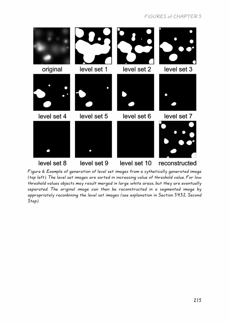
FIGURES of CHAPTER 5
215
Figure 6. Example of generation of level set images from a sythetically generated image (top left). The level set images are sorted in increasing value of threshold value. For low threshold values objects may result merged in large white areas, but they are eventually separated. The original image can then be reconstructed in a segmented image by appropriately reconbining the level set images (see explanation in Section 5.4.3.2, Second Step).

FIGURES of CHAPTER 5
216
Figure 7. Area opening applied to grey-scale images. In the first step, the image is thresholded at different levels (sample F369/1, lead map of Figure 2.d).

FIGURES of CHAPTER 5
217
Figure 8. Area opening applied to grey-scale images. In the second step, individual objects appearing in the level images obtained at the first step (Figure 7) are identified and labelled according to their area.

FIGURES of CHAPTER 5
218
Figure 9. In the final step, the labelling process combines all the labelled images of the previous step (Figure 8) according to formula (7). In the resulting segmented image (a), in practice each object is labelled according to its volume ion yield. The corresponding size distribution (b) is calculated as the histogram of the segmented image.
Figure 10. Example images of the application of area opening to SIMS images (a1, b1, c1). Area opening segments objects, and labels them with colours that represent their ‘volume ion yields’ (a3, b3, c3). The choice of the values of parameters of bilateral filtering (here, σs = 6, σt = 2) affects the output segmented images and the corresponding size distributions (a4, b4, c4). The segmented images are scaled to the same intensity range to facilitate the comparison. The images after application of bilateral filtering (a2, b2, c2) are shown for comparison. (Samples F216a/1 and F296/2).

FIGURES of CHAPTER 5
219
Figure 11. Comparison of results of area opening on SIMS images of lead and calcium with a SEM-BSE image (a) acquired on the same sample area (sample F216a/1). In the BSE image lead particles appear in light grey, and calcium particles in dark grey. The large elongated particle is menilite. The outlines, obtained for lead and calcium particles respectively from images 10.a3 and 10.b3, are overlaid on the BSE image respectively in (b) and (c), For better clarity, outlines are represented with different colours, and small details were removed.

FIGURES of CHAPTER 5
220
Figure 12. Comparison of results of area opening on SIMS image of barium with a SEM-BSE image (a) acquired on the same sample area (sample F296/2). In the BSE image barium particles appear in medium grey (indicated by the arrow). In (b) the SIMS map of barium (in green) was overlaid on the BSE image, showing that the ion yields in SIMS reflect the morphological structure of a large particle. The outlines obtained for barium particles from the segmented image of Figure 10.c3 are overlaid on the BSE image in (c), The overlay shows that the substructure of the particle is retained in the segmented image.

FIGURES of CHAPTER 5
221
Figure 13. SEM-BSE image (a) and EDX maps of lead (b) and calcium (c) (sample F216a/1). The mapped area is the same as for the SIMS maps of Figures 10.a and 10.b. Due to poorer lateral resolution compared to SIMS, SEM-EDX maps are generally less detailed. The map of lead (b), corresponding to the main paint component, clearly exhibits a lower contrast.

FIGURES of CHAPTER 5
222
Pb Ca Ba
Figure 14. Figures 14-18 represent summary images of the segmented images obtained by application of area opening on SIMS maps of ground paints in paintings by Van Gogh. In each image lead, calcium, and barium are represented respectively in red, blue, and green. The paint cross-sections are outlined in white; regions of interest in the ground paint used for the analysis are outlined in yellow.

FIGURES of CHAPTER 5
223
Pb Ca Ba
Figure 15. Summary image of application of area opening to SIMS images of ground paints.

FIGURES of CHAPTER 5
224
Pb Ca Ba
Figure 16. Summary image of application of area opening to SIMS images of ground paints.

FIGURES of CHAPTER 5
225
Pb Ca Ba
Figure 17. Summary image of application of area opening to SIMS images of ground paints.

FIGURES of CHAPTER 5
226
Figure 18. Summary image of size distributions obtained after application of area opening to SIMS images of ground paints. Size distributions for lead (in red), calcium (in blue), and barium (in green) are represented for each acquisition in a single bar plot, with bars grouped according to ion yield volume classes.

FIGURES of CHAPTER 5
227
Qualitative
classification
Quantitative classification
colour composition texture
Sample Code
Pb Ca Ba
F216a/1 * 1 1 1 / 2 * 2 / 5 2 / 5 0
F216b/1 1 2 2 2 / 5 2 / 5 0
F216d/1 2a 1 3 2 3 / 0 4
F216e/1 2a 2 3 2 0 4
F216f/2 2a 1 1 2 1 0
F216j/1 2a 1 3 1 / 5 1 / 2 / 5 4
F267/2 2b 2 3 2 1 / 2 / 5 4
F294/1 2b 2 3 2 5 4
F296/2 2b 2 3 2 / 5 3 (or 0) 4
F369/1 extra 1 1 / 2 2 / 5 2 / 3 0
* contains menilite
Table 1. Summary of the classifications of the ground paints. The qualitative classification was made by examination of support, paint surface, and paint cross-sections (see Chapter 1). The quantitative classification was made separately on the basis of colour, composition, and texture of the paint at the microscopic level. The numbers correspond to classes as follows (for the same sample multiple numbers are shown when different acquisitions are assigned to different classes). Qualitative classification: 1 = white grounds, 2a = grey grounds, batch A, 2b = grey grounds, batch B. Colour: 1 = light-coloured grounds, 2 = grey grounds. Composition: 1 = lower Ca/Pb, 2 = higher Ca/Pb, 3 = Ba rich. Texture: 0 = no element present, 1 = bimodal distribution, small particles predominant, 2 = bimodal distribution, large particles predominant, 3 = unimodal distribution, small particles, 4 = unimodal distribution, large particles, 5 = uniform distribution.


FIGURES of CHAPTER 6
229
Figure 1. BSE image of sample F216j/1 acquired after gold coating (30 nm) and NanoSIMS analysis. The analysed area, where the gold layer has been sputtered, is clearly visible. A close-up shows the damage caused by the sputtering beam.
Figure 2. NanoSIMS maps of oxygen, chlorine, nitrogen (detected as CN- where carbon is also present), and sodium. The ground paint layer and the cardboard fibres are highlighted respectively in the maps of oxygen and chlorine, and in those of nitrogen and sodium. Oxygen is associated to lead white, calcium carbonate, gypsum, and barite.
Chlorine is a marker for the lead white present in the ground paint. Nitrogen and is indicative of protein residual in the fibres or of glue that might have been used in the manufacturing of the cardboard. Sodium can be naturally present in the fibres or might have been introduced during the manufacturing process for softening the pulp.

FIGURES of CHAPTER 6
230
Figure 3. Images of sulphur indicate gypsum and barite particles (where there is co-occurrence with calcium and barium). The overlay of sulphur, barium and calcium represented in the bottom right corner represents particles of barite (in magenta), gypsum (in yellow) and calcium carbonate (in green). The thin line of sulphur (in red in the overlay) lies in the contact zone of the ground paint layer with the cardboard (compare BSE image of Figure 4). Sulphur was likely absorbed by the cardboard from the atmosphere and had subsequently reacted with lead in the ground paint to form lead sulphate.

FIGURES of CHAPTER 6
231
Figure 4. Barium and
strontium (Figure 5) exhibit
heterogeneous distributions
with differences in relative
concentrations between- and
within-particles.
Figure 5. Barium (Figure 4) and
strontium exhibit heterogeneous
distributions with differences
in relative concentrations between- and
within-particles. between- and
within-particles.


APPENDIX A
234
Figure A.1. Plaster figure of a female torso (F216a, mid. June 1886; Van Gogh Museum, Vincent van Gogh Foundation, Amsterdam)
Figure A.2. Plaster figure of a female torso (F216b, mid. June 1886; Van Gogh Museum, Vincent van Gogh Foundation, Amsterdam)
Figure A.3. Plaster figure of a female torso (F216d, mid. June 1886; Van Gogh Museum, Vincent van Gogh Foundation, Amsterdam)
Figure A.4. Plaster figure of a male torso (F216e, mid. June 1886; Van Gogh Museum, Vincent van Gogh Foundation, Amsterdam)

APPENDIX A
235
Figure A.5. Plaster figure of a kneeling muscular model (F216f, mid. June 1886; Van Gogh Museum, Vincent van Gogh Foundation, Amsterdam)
Figure A.6. Plaster figure of a female torso (F216j, mid. June 1886; Van Gogh Museum, Vincent van Gogh Foundation, Amsterdam)
Figure A.7. Self-portrait with straw hat (F267, March-June 1887; Van Gogh Museum, Vincent van Gogh Foundation, Amsterdam)
Figure A.8. Portrait of Theo (F294, Summer 1887; Van Gogh Museum, Vincent van Gogh Foundation, Amsterdam)

APPENDIX A
236
Figure A.9. Self-portrait with felt hat (F296, Summer 1887; Van Gogh Museum, Vincent van Gogh Foundation, Amsterdam)
Figure A.10. Woman by a cradle, portrait of Leonie Rose Davy-Charbuy (F369, August-September 1887; Van Gogh Museum, Vincent van Gogh Foundation, Amsterdam)
Figure A.11. The hill of Montmartre with quarry (F229, Fall 1886; Van Gogh Museum, Vincent van Gogh Foundation, Amsterdam)
Figure A.12. The hill of Montmartre with quarry (F230, Fall 1886; Van Gogh Museum, Vincent van Gogh Foundation, Amsterdam)


APPENDIX B
238
Figure B.1. BSE images of sample F216a/1, overview (top) and detail (bottom).
Figure B.2. BSE images of sample F216b/1, overview (top) and detail (bottom).

APPENDIX B
239
Figure B.3. BSE images of sample F216d/1, overview (top) and detail (bottom).
Figure B.4. BSE images of sample F216e/1, overview (top) and detail (bottom).

APPENDIX B
240
Figure B.5. BSE images of sample F216f/2, overview (top) and detail (bottom).

APPENDIX B
241
Figure B.6. BSE images of sample F216j/1, overview (top), and detail (bottom). The images were taken after analysis by nanoSIMS.
Figure B.7. BSE images of sample F216a/1, overview (top) and detail (bottom).

APPENDIX B
242
Figure B.8. BSE images of sample F267/2, overview (top) and detail (bottom).
Figure B.9. BSE images of sample F294/1, overview (top) and detail (bottom).

APPENDIX B
243
Figure B.10. BSE images of sample F296/2, overview (top) and detail (bottom).

APPENDIX B
244
Figure B.11. BSE images of sample F369/1, overview (top) and detail (bottom).


APPENDIX C
246
Figure C.1.
Figure C.2.
Figure C.3. Figures C.1-C.3: processing of SIMS maps of lead (top row) and calcium (bottom row) for sample F216a/1 in three areas (Fig. C.1 = area A, Fig. C.2 = area B, Fig. C.3 = area C) for measurement of particle size distribution. From left to right, the image before processing, after bilateral filtering, after area opening, and the resulting particle size distribution.

APPENDIX C
247
Figure C.4.
Figure C.5.
Figure C.6.

APPENDIX C
248
Figure C.7. Figures C.4-C.7: processing of SIMS maps of lead (top row) and calcium (bottom row) for sample F216d/1 in four areas (Fig. C.4 = area A, Fig. C.5 = area B, Fig. C.6 = area C, Fig. C.7 = area D) for measurement of particle size distribution. From left to right, the image before processing, after bilateral filtering, after area opening, and the resulting particle size distribution.

APPENDIX C
249
Figure C.8.
Figure C.9. Figures C.8-C.9: processing of SIMS maps of lead (top row) and calcium (bottom row) for sample F216d/1 in two areas (Fig. C.8 = area A, Fig. C.9 = area B) for measurement of particle size distribution. From left to right, the image before processing, after bilateral filtering, after area opening, and the resulting particle size distribution.
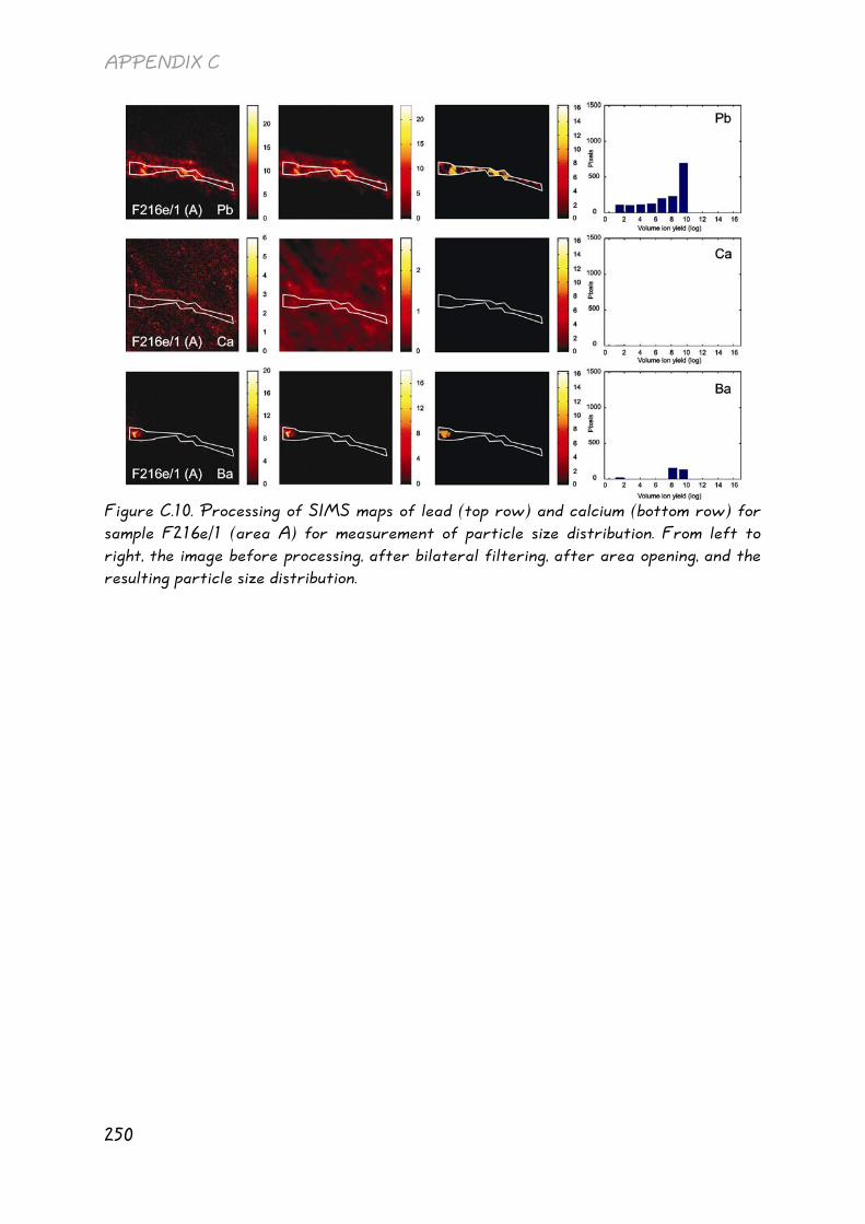
APPENDIX C
250
Figure C.10. Processing of SIMS maps of lead (top row) and calcium (bottom row) for sample F216e/1 (area A) for measurement of particle size distribution. From left to right, the image before processing, after bilateral filtering, after area opening, and the resulting particle size distribution.

APPENDIX C
251
Figure C.11.
Figure C.12. Figures C.11-C.12: processing of SIMS maps of lead (top row) and calcium (bottom row) for sample F216f/2 in two areas (Fig. C.11 = area A, Fig. C.12 = area B) for measurement of particle size distribution. From left to right, the image before processing, after bilateral filtering, after area opening, and the resulting particle size distribution.

APPENDIX C
252
Figure C.13.
Figure C.14.

APPENDIX C
253
Figure C.15. Figures C.13-C.15: processing of SIMS maps of lead (top row) and calcium (bottom row) for sample F216j/1 in three areas (Fig. C.13 = area A, Fig. C.14 = area B, Fig. C.15 = area C) for measurement of particle size distribution. From left to right, the image before processing, after bilateral filtering, after area opening, and the resulting particle size distribution.
Figure C.16.

APPENDIX C
254
Figure C.17.
Figure C.18. Figures C.16-C.18: processing of SIMS maps of lead (top row) and calcium (bottom row) for sample F267/2 in three areas (Fig. C.16 = area A, Fig. C.17 = area B, Fig. C.18 = area C) for measurement of particle size distribution. From left to right, the image before processing, after bilateral filtering, after area opening, and the resulting particle size distribution.

APPENDIX C
255
Figure C.19. Processing of SIMS maps of lead (top row) and calcium (bottom row) for sample F294/1 (area A) for measurement of particle size distribution. From left to right, the image before processing, after bilateral filtering, after area opening, and the resulting particle size distribution.

APPENDIX C
256
Figure C.20.
Figure C.21. Figures C.20-C.21: processing of SIMS maps of lead (top row) and calcium (bottom row) for sample F296/2 in two areas (Fig. C.20 = area A, Fig. C.21 = area B) for measurement of particle size distribution. From left to right, the image before processing, after bilateral filtering, after area opening, and the resulting particle size distribution.

APPENDIX C
257
Figure C.22.
Figure C.23.

APPENDIX C
258
Figure C.24..
Figure C.25. Figures C.22-C.25: processing of SIMS maps of lead (top row) and calcium (bottom row) for sample F369/1 in three areas (Fig. C.22 = area A, white paint layer,, Fig. C.23 = area A, beige paint layer, Fig. C.24 = area B, Fig. C.25 = area C) for measurement of particle size distribution. From left to right, the image before processing, after bilateral filtering, after area opening, and the resulting particle size distribution.

259
To establish a chronology of paintings or prove the authenticity of a picture, it is important for conservators and art historians to differentiate and classify different formulations and production batches of supports, grounds, and paints. This is particularly true in 19th century, since ready-made artists’ materials are commercially available to painters thus obscuring the individual material signature, that is, the hand of painters. In the making of paint for grounds, the workability of the ground paint translates itself into factors like the ratio of pigment and filler materials, the choice of binding medium, drying properties, spreadibility, absorbency, layer thickness and opacity. The adhesion of the upper paint layer onto the ground layer is another major factor of importance. These properties are embedded in paintings in the form of still measurable units such as layer build-up and texture, i.e. the microscopic distribution of constituents and their composition. In this Thesis we explore quantitative methods of classification based on imaging microscopic data of paint cross-sections. The quantitative character of the approach overcomes the limitations of qualitative analysis, especially when comparing objects of similar characteristics. Software was specifically developed in Matlab® to process the datasets, to extract and to measure relevant features that could lead to an effective discrimination between samples of similar characteristics. The method was applied to the case study of selected ground paints in a group of paintings made by Van Gogh on commercially pre-primed carton supports during his Paris period (1886-1887). The paintings in question were six studies of plaster-cast statuettes (F216a, F216b, F216d, F216e, F216f, F216j) dated to mid. June 1886, and three tiny portraits (F267, F294, F296), dated to 1887. A random control sample of ground from an 1887 portrait on canvas (F369) was included. The ground paints on carton are thought to be similar on the basis of qualitative macroscopic and microscopic examination of the primed supports, carried out by the head restorer Ella Hendriks of the Van Gogh Museum and her team. Their analysis was based on

SUMMARY
260
colour, build-up, composition and surface texture of the ground paints, and the size, composition, and features of construction of the cardboard supports. An imaging Secondary Ion Mass Spectrometer (static-SIMS) and a light microscope interfaced with a digital camera at AMOLF were used under standardized conditions to acquire the data used for the comparison. Scanning Electron Microscopy combined with Energy Dispersive X-ray analysis (SEM-EDX) and Gas Chromatography - Mass Spectrometry (GC-MS) were used in addition to validate the results of SIMS and to answer some specific questions. SIMS, an extremely useful and efficient method of examination of the layer structure of paintings in cross-section, allows mapping of both the inorganic and organic components at high lateral resolution. SIMS gives a more accurate rendering of the materials present at the surface, because, in contrast to SEM-EDX, it probes only the upper 5 nm. Although the software was specifically developed to be used on SIMS data and digital colour images, it can be adapted to process other types of imaging datasets. In Chapter 2 we discuss the data obtained by imaging SIMS on the paint cross-sections under study. SIMS data show that there are clear differences in composition and compound texture between the paints of the grounds. Qualitatively we can distinguish two types of ground formulations, one consisting of a simple mixture of lead white and calcium carbonate (F216a and F216b), and a second one consisting of a mixture of lead white, calcium carbonate or gypsum, and barium sulphate (F216d, F216e, F216f, F216j, F267, F294, F296). Barium sulphate is present in its natural form, barite, as it is found in association with strontium sulphate. Calcium carbonate is found in samples F216a/1, F216b/1, F294/1, and gypsum in samples F216f/2, F216j/1, F267/2, F369/1. There does not seem to be any calcium carbonate or gypsum in detectable amounts in sample F216e/1. It is also uncertain whether sample F216d/1 contains calcium carbonate, and whether sample F296/2 contains calcium carbonate and/or gypsum. Sample F369/1 from a painting on canvas should be considered as a third type of ground, because of its different colour and other visual features (see Chapter 1). However, from a compositional point of view, this sample appears under SIMS to belong to the second group, since the detected amounts of earth pigments that provide the beige tint of the first ground layer do not differ from those seen in the other samples. The data (SIMS as well as GC-MS) show that the binding medium in the ground paints under investigation do not consist of oil alone. The identified lauric and myristic acid suggest other contributions of fats, possibly by addition of egg- or milk-derived products, presumably with the aim of making a more absorbent ground. A peculiar finding in one of the grounds (F216a/1) is that of a large particle of the magnesium-rich variety of opaline silica called menilite, which is found only in the

SUMMARY
261
Paris Basin and in very few other locations. Its presence suggests that the menilite marls from between the two main gypsum masses mined in Paris were used in the preparation of the ground paint. The Paris Basin is a rich source of gypsum, limestone, and clay, and thus a likely source for some of the materials used in ground paints by the colourmen of Paris. Impure materials might have been used, especially for cheap-grade ground paints as those of carton supports, which are intended for study purposes by artists. Such impurities may also impart a tint or a colour to the material. Therefore, at least in some cases, some materials that are found in the paint in minute or small amounts might have been introduced along with a main paint component rather than added as separate substances. In Chapters 3, 4, and 5 quantitative comparisons of the ground paints are made on the basis of different characteristics, measured at the microscopic level. Image processing and pattern recognition techniques have been employed to enhance and extract this information from the samples. The features considered were the colour content of light microscopic images of samples (Chapter 3), the material composition of the ground paints derived from SIMS data (Chapter 4), and the texture of the paint characterized by elemental distribution of particles in SIMS images (Chapter 5). In Chapter 3 we compare the ground paints on the basis of their colour as seen in light-microscopic images of the paint cross-sections. Colour histograms were used to represent the colour information of the ground paints. The similarity between the colours of the paints was measured by calculating a weighted distance between the histograms, and their classification was obtained with hierarchical clustering techniques. The ‘distance’ adopted has been used successfully before in systems of image query and retrieval from databases. Colour content analysis was able to divide the supports into two different groups, one consisting of grey grounds (F216b, F216e, F267, F294, and F296) and one of lighter coloured grounds (F216a, F216d, F216f, F216j, and F369). The distinction between the two identified groups of ground paints is based on differences in brightness. Slight tint differences have a low impact on the classification, as well as the few or small dark-coloured particles because of their small contribution to the paint cross-section area. These small or few dark coloured particles get a very high discriminating weight in a qualitative subjective classification because they are very striking to the human eye. The classification complements the one obtained by traditional techniques, since they are obtained from different types of data. One aspect to bear in mind is that the colour of paint in a cross-section and the colour of the paint surface are related in a

SUMMARY
262
complex way because of the joint end result of multiple absorption, transmission and scattering interactions of light within the paint layer. In general the same surface colour can be achieved with different formulations, whereby the colour, composition, and micro-structural properties of the paint materials may vary, so that paints that are macroscopically similar might differ at the microscopic scale. For example relatively few dark particles in a light matrix may produce the same surface colour as a layer that is more uniformly tinted at the microscopic level. Therefore the colour of the ground is just one factor for the colour analyst of paintings to consider in questions on the artistic production process and the authenticity of paintings. In Chapter 4, the methodology used in Chapter 3 is adapted to processing of imaging SIMS data as a means to compare composition information. Data reduction and feature extraction were essential steps to reduce data complexity and computational effort, to extract relevant discriminating features, and to improve the quality of the classification. Characteristic elements identified in Chapter 2 (lead, calcium, barium, strontium, iron, aluminium) were hand-selected from the spectral data, regions of interest within the ground paint area were traced, and Principal Component Analysis was used for further data reduction. The resulting imaging data sets were then processed in the same fashion as the colour images in Chapter 3. The results of the application to the case study show that the discriminating features were preserved even after strong data simplification. Compositional classes could be identified, and a valid classification was obtained. The ground paints were classified according to three groups: one class corresponding to samples containing barium (F216d/1, F216e/1, F216j/1, F267/2, F294/1, F296/2); the other two, very similar yet showing a small degree of distinction, to samples with no or negligible amount of barium and with different relative abundances of calcium to lead (F216a/1 and F216f/2, and F216b/1). The ground layers of the control sample F369/1 are attributed to the last two classes. The methodology highlighted compositional features that can be essentially reduced to the most abundant elements in the paint (lead, calcium, and barium). The quantitative classification based on composition matches closely the one obtained by traditional comparative methods, as in the latter barium sulphate was considered highly discriminating for the grounds. The results also follow the anticipations of qualitative examination of the unprocessed SIMS data. In addition the quantitative classification captured slighter differences in relative ratio of calcium and lead, which could have not been easily perceived with a qualitative comparison.

SUMMARY
263
The size of the particles of the materials used in paint affect many properties of the paint, such as colour and workability. It can influence the mode of application of upper paint layers and contribute to the creation of surface textural effects. In Chapter 5 we quantify the texture of constituents of the main ground paint components from SIMS elemental distribution maps. Characteristic elements (lead, calcium, barium) identified in Chapter 2 were hand-selected from the spectral data, and regions of interest within the ground paint area were traced. Data was preprocessed with bilateral filtering and particle size distributions were obtained by area opening. The method proved to be able to identify texture, structure and substructure of particles, and showed flexibility in measuring texture and structure at different scale levels, by appropriate choice of the processing parameters. The texture of the ground paints is found to be a highly discriminating feature in this research. The paints exhibit greater differences than could have been observed from the other classifications. The calcium-containing materials show the largest degree of variability. The main paint component lead white generally exhibits the same type of size distribution in all samples, with presence of large particles intermixed with small particles, typical for the Dutch ‘stack’ process (carried out corroding lead in pots stacked and buried in horse manure). However differences between samples within this type of distribution can be observed. Barium sulphate is in general consistently present as coarse particles, so that there are no qualitative differences in the size distributions for this material. In Chapter 6 we explore the potential of a new generation of ion microprobes - the NanoSIMS - on one of the paint cross-sections (sample F216j/1) examined in the earlier chapters. The higher spatial and mass resolution combined with higher secondary ion collection efficiency provided additional information that could not be obtained by the SIMS at AMOLF. These include the enhanced detection of fine sub-structural details within barite particles and of other fine structures in key trace elements and organic markers in the paint cross-section. NanoSIMS was able to detect differences in relative concentrations of strontium to barium, examine the distribution of barium and strontium within and between barite particles, and perform isotope analysis of strontium in barites. Strontium and sulphur isotopic ratios seem promising tools for the distinction of different sources barite. More extensive work on barite in paints involving the development/consultation of a database of barites from different localities is required. In addition a remarkable distribution was found for a micron thin layer of sulphur containing material on the contact between the cardboard and the lead white containing ground paint. Could this be atmospheric sulphur that is embedded and trapped by the lead? Further studies of its isotopic composition is certainly worthwhile.

SUMMARY
264
As final conclusion, we can state that the combined examination of the results obtained for these case studies demonstrates that the ground paints were prepared in different batches even if the preparation is aimed at imparting the same qualities.
COMMENTS A general observation to be made from this work is that a quantitative classification of samples may only partly follow the one made using the more traditional qualitative criteria. This can be explained by the fact that different types of data were used, and that different features were considered in each case, so that samples were assigned to different groups depending upon the particular criteria considered. However different characteristics at the microscopic and macroscopic level are not independent, so that for example colour, composition, and texture at both length scales are interrelated in a complex way. Further work should therefore aim to develop a classification procedure based on the ensemble of the features considered - colour, composition, and texture - rather than on individual features alone. The drawing of appropriate conclusions from such cumulative data depends of course heavily on the expertise and the connoisseurship of the paint specialist who has to weigh the significance of the various types of evidence gathered. This new method for quantitative characterisation of paint samples is envisaged as a complementary tool, supplementing the traditional qualitative approach. Potentially it enables a more systematic and precise analysis of microscopic features in ground and paint samples. The method could be used to understand how these features affect the visual and working properties of these materials, and in relation to that the influence of the substrate on the application of successive paint layers and on the painting style. Another potential application is the investigation of the discolouration of paints in paint cross-sections and its impact on the visual appearance of the painted surface. The method could also aid a classification of the materials used by different schools, or painters, at different moments in time. Observations made in this research indicate that sufficient sampling statistics is of critical importance for inhomogeneous samples, especially when materials present in relatively low concentrations are considered. Many questions on a painting are answered with the examination of a single paint cross-section, which an approximate size of 100 μm. It has not yet been established however for which characteristics and to what extent such a minuscule sample can be considered as

SUMMARY
265
being representative of the entire painting. In addition, we have observed that paint cross-sections generally show a different appearance after repolishing. Materials that are present in low concentrations might not be visible in the paint cross-section surface or in the analysed area. The significance of the observations made on the particular sectioned surface under analysis should be assessed critically, especially when the results are to be used in a comparative study. To address these issues a detailed study should involve repeated polishing of several cross-sections taken from different paintings, from different spots in each painting, and from paint reconstructions. The methodologies presented in this Thesis may be used to measure between-painting, within-painting, and within-sample variability. The use of techniques such emerging X-ray nano-tomography would help addressing these issues without the need for repeated polishing of a sample.


267
Om de chronologie van de schilderijproductie of de authenciteit van een schilderij te kunnen vast stellen is het belangrijk voor restauratoren en kunsthistorici om de verschillen in samenstelling en formulering van de drager, grondering en verf te kunnen onderscheiden en classificeren. Dit vooral van belang in de 19e eeuw waarin kant-en-klare kunstenaarsmaterialen commercieel beschikbaar komen en de hand van de individuele schilder daardoor minder zichtbaar wordt. Bij de het maken van de grondverf is de verwerkbaarheid van de grondverf te vertalen in materiaalkeuze, bindmiddelen, spreidbaarheid, absorberend vermogen, drogende eigenschappen, laagdikte, en opaakheid. Ook de hechting van de bovenliggende verf aan de grondering is een belangrijk punt. Deze eigenschappen zijn in schilderijen vastgelegd in de vorm van de nu nog meetbare laagopbouw, textuur i.e. microscopische verdeling van de grondstoffen en hun samenstelling. In dit Proefschrift exploreren wij kwantitatieve classificatiemethoden, die gebruik maken van microscopische verdelingskaarten van materialen in schilderijdwarsdoorsneden. Het kwantitatieve karakter van de aanpak overwint de beperkingen van de nu gebruikelijke kwalitatieve analyse, in het bijzonder wanneer objecten van erg op elkaar lijkende samenstelling moeten worden vergeleken. Software werd ontwikkeld in een Matlab® omgeving om de gegevens te kunnen bewerken, en relevante eigenschappen te kunnen extraheren en meten, die zouden kunnen leiden tot een effectief onderscheid tussen nauw verwante korrelverdelingen. De methode is toegepast op grondverfmonsters genomen uit een groepje schilderijen van Van Gogh gemaakt op commercieel reeds voor-gegrondeerde dragers op karton (z.g. cartons) tijdens zijn Parijse periode (1886-1887). De onderhavige schilderijen zijn zes studies van gipsen beeldjes (F216a, F216b, F216d, F216e, F216f, F216j) gedateerd in midden juni 1886 en drie portretjes (F267, F294, F296) gedateerd in 1887. Daaraan werd een willekeurig gekozen monster van een grondverf toegevoegd als controlemonster dat afkomstig was uit een portret op canvas (F369). De

SAMENVATTING
268
grondverf op de cartons worden als erg op elkaar lijkend beschouwd op basis van kwalitatief macroscopisch en microscopisch onderzoek van de gronderingen door hoofdrestaurator Ella Hendriks en haar team in het Van Gogh museum. Hun analyse maakte gebruik van kleur, opbouw, samenstelling en oppervlaktetextuur van de grondverf en tevens de maat, samenstelling en eigenschappen van de kartonnen dragers. Op AMOLF werd een imaging secundaire ionen massaspectrometer (static-SIMS) en een lichtmicroscoop verbonden met een digitale camera gebruik onder gestandaardiseerde omstandigheden om de gegevens binnen te halen, die voor het vergelijkend onderzoek nodig waren. Daarnaast werd Scanning Electronen Microscopie (SEM) gecombineerd met Energie Dispersieve Röntgen analyse (EDX) en Gaschromatografie-Massaspectrometrie ingezet om de uitkomsten van de SIMS data te verifiëren en enige bijzondere vragen te kunnen beantwoorden. SIMS, een uiterst bruikbare en efficiënte manier van onderzoek van de laagstructuur in verfdwarsdoorsnedes, maakt het mogelijk om zowel de anorganische als organische bestanddelen met hoge laterale resolutie in kaart te brengen. SIMS geeft vergeleken met SEM-EDX een nauwkeuriger beeld van de verdeling van materialen aan het oppervlak, omdat in tegenstelling tot SEM slechts de bovenste 5 nanometer analytisch in beeld wordt gebracht. Overigens is de beeldbewerkingsoftware weliswaar ontwikkeld voor SIMS and digitale kleurgegevens, maar ze kan ook worden aangepast voor de verwerking van andere soorten beeldgegevens. In Hoodstuk 2 worden de gegevens bediscussieerd, die werden verkregen door toepassing van imaging SIMS op de schilderijdwarsdoorsnedes. De SIMSgegevens tonen aan dat er duidelijke verschillen zijn in samenstelling en verdeling van de materialen in de gronderingen. Kwalitatief zijn twee typen formulering van de grondverf te onderscheiden: de ene bestaat uit een eenvoudig mengsel van loodwit en calciumcarbonaat (F216a/1 en F216b/1) en de tweede bestaat uit mengsels van loodwit, calciumcarbonaat of gips en bariumsulfaat (F216d/1, F216e/1, F216f/2, F216j/1, F267/2, F294/1, F296/2). Bariumsulfaat is in zijn natuurlijke vorm aanwezig, omdat de bariet ook strontium bevat. Calciumcarbonaat wordt gevonden in de monsters F216a/1, F216b/1, F294/1 en gips in F216f/2, F216j/1,F267/2,F267/2, F369/1. Er is geen spoor van calciumcarbonaat of gips gevonden in F216e/1. Het is ook onzeker of monster F216d/1 calciumcarbonaat bevat en of F296/2 calciumcarbonaat en/of gips bevat. Het monster F369/1 uit het canvasschilderij is eigenlijk een derde type grondering vanwege de verschillen in kleur en andere visueel waar te nemen eigenschappen (zie Hoofdstuk 1). Maar dit monster is vanuit het oogpunt van samenstelling bepaald met SIMS, een grondering van de tweede categorie, omdat de hoeveelheid aardpigmenten, die de beige tint geven aan de eerste (bovenste) grondverflaag niet erg verschilt van die in de andere monsters. De

SAMENVATTING
269
gegevens (SIMS en ook GC-MS) zeggen dat het bindmiddel in de sommige grondverfmonsters niet alleen maar drogende olie bevat. Het geïdentificeerde laurine- en myristine-vetzuur suggereert de aanwezigheid van andere vetten - mogelijk een toevoeging van ei of melk componenten - die kunnen zijn ingemengd om de grondering wat meer absorberend te maken. Een bijzondere vondst in één van de gronderingen (F216a/1) is een groot deeltje van de magnesiumrijke variëteit van opalien silicaat, die meliniet wordt genoemd. Dit mineraal wordt alleen gevonden in gesteenten van het Bekken van Parijs en op sommige andere ver verwijderde locaties. De aanwezigheid van meliniet in de grondverf suggereert dat de meliniet-houdende mergels, die voorkomen tussen de twee grote gemijnde gipsvoorkomens bij Parijs, direct zijn gebruikt voor de bereiding van de grondverf. Het Bekken van Parijs is een rijke bron van gips, kalk, en klei en dus een voor de hand liggende bron van grondverfmateriaal voor de verfmakers in Parijs. Onzuivere materialen kunnen vooral gebruikt zijn in de grondverf op de goedkope cartons, die voor studie te koop werden aangeboden. Zulke onzuiverheden dragen bij aan de tint of kleur van de materialen en de verf. Daarom kunnen, althans in sommige gevallen, de materialen, die in kleine hoeveelheden in de verf zijn aangetroffen samen met de hoofdkomponenten zijn geïntroduceerd en niet zozeer apart zijn toegevoegd. In Hoofdstukken 3, 4 en 5 worden kwantitatieve vergelijkingen gemaakt van de grondverven op basis van verschillende met microscopie gemeten eigenschappen. Beeldverwerkings en patroonherkenningstechnieken zijn toegepast om deze informatie uit de monsters naar voren te halen en te versterken. De in beschouwing genomen eigenschappen waren de kleurigheid van de microscopische beelden (Hoofdstuk 3), de materiële samenstelling van de grondverftypen bepaald met SIMS (Hoofdstuk 4), en de verftextuur gebruikmakend van de verdelingskaarten elementen in de SIMS data (Hoofdstuk 5). In Hoofdstuk 3 vergelijken we de grondverf op basis van de kleur in de lichtmicroscopische beelden van de verfdwarsdoorsnedes door gebruik te maken van kleurhistogrammen. De vergelijkbaarheid van de verfkleuren werd gemeten door de berekening van de gewogen afstand tussen de histogrammen en hun klassificatie werd verkregen met behulp van hiërarchische clusteringstechnieken. Deze “afstand” is al eerder succesvol gebruikt bij het opbergen en terugvinden van beelden in databases. De kleurgehalte-analyse kon de grondverftypen verdelen in twee groepen. Een groep van grijze gronderingen (F216b, F216a, F267, F294 en F296) en een groep van lichter gekleurde gronderingen (F216a, F216d, F216f, F216j en F369). Het verschil tussen deze groepen is gebaseerd op helderheid. Kleine tintverschillen

SAMENVATTING
270
en ook de weinige kleine donkergekleurde deeltjes hebben geringe invloed op de classificatie omdat ze maar weinig bijdragen in het totale beeldoppervlak van de dwarsdoorsnedes. Deze gering voorkomende kleurrijke deeltjes krijgen een sterk discriminerende waarde in een kwalitatieve subjectieve classificatie omdat ze sterk voor het oog opvallen. De gevonden berekende classificatie complementeert degene die verkregen met de traditionele methode, omdat ze verkregen zijn met andere gegevens. Hierbij moeten we bedenken dat de kleur van een verfdwarsdoorsnede en de kleur van het verfoppervlak op een complexe manier met elkaar in verhouding staan vanwege het samenspel van meervoudige absorptie, transmissie en verstrooiing van licht in de verflaag. In het algemeen kan dezelfde oppervlaktekleur worden verkregen door verschillende formuleringen waarbij kleur, samenstelling en microstructurele eigenschappen van de verfmaterialen kunnen verschillen zodat de verf die macroscopisch hetzelfde lijkt op microscopische schaal kan verschillen. Een paar donkere deeltjes in een lichtgekleurde laag bij voorbeeld geven dezelfde oppervlaktekleur als een laag, die meer uniform getint is op microscopisch niveau. Daarom is kleur van de grondering slechts een van de factoren die kleuronderzoekers van schilderijen moeten meenemen bij vragen over het artistieke produktieproces en authenticiteit. In Hoofdstuk 4 pasten we de methodologie uit Hoofdstuk 3 toe op imaging SIMS gegevens ten behoeve van het vergelijken van informatie over de samenstelling. Datareductie en kenmerkextractie waren essentiële stappen om de complexiteit van data te reduceren en de berekeningsinspanning te verkleinen, de relevante onderscheidende kenmerken naar voren te halen en de kwaliteit van de classificatie te verbeteren. Karakteristieke elementen die in Hoofdstuk 2 zijn geïdentificeerd (lood, calcium, barium, strontium, ijzer en aluminium) werden handmatig geselecteerd uit de spectrale gegevens, interessegebieden binnen de grondering werden getraceerd en Principale Componenten Analyse werd gebruikt voor verdere data reductie. De resulterende datasets werden vervolgens op dezelfde wijze verder bewerkt als de kleurbeelden in Hoofdstuk 3.De resultaten van toepassing op de casus tonen aan dat de discriminerende kenmerken zelfs na sterke data vereenvoudiging nog steeds aanwezig waren. Samenstellingsgroepen konden worden geïdentificeerd en een waardevolle classificatie werd verkregen. De grondverven werden in drie groepen verdeeld: één groep correspondeert met monsters, die barium bevatten (F216d/1, F216e/1, F216j/1, F267/2, F294/1, F296/1). De twee andere groepen, die vergelijkbaar zijn maar toch wat verschil vertonen, corresponderen met monsters met verschillende relatieve verhoudingen calcium en lood, en geen of te verwaarlozen hoeveelheden barium (F216a/1, F216b/1, F216f/2). De grondlagen in controlemonster F369 behoren tot de laatste twee groepen. De methodologie bracht

SAMENVATTING
271
samenstellingselementen naar voren die behoren tot de hoofdelementen in de verf (t.w. lood, calcium en barium). Deze kwantitatieve classificatie gebaseerd op samenstelling komt nauw overeen met de indeling op basis van traditionele methoden, omdat in de laatste indeling bariumsulfaat werd beschouwd als een sterk onderscheidende factor. De resultaten bevestigen ook de verwachtingen uit het kwalitatieve onderzoek van de SIMSgegevens. Bovendien haalt de kwantitatieve classificatie kleinere verschillen in de relatieve verhouding van calcium en lood naar voren, die niet makkelijk te zien zijn bij een kwalitatieve vergelijking. De grootte van de deeltjes in verf beïnvloeden veel verfeigenschappen, waaronder kleur en verwerkbaarheid. Het kan de manier van aanbrengen van de bovenste verflagen beïnvloeden en bijdragen aan het maken van oppervlakkige texturele effecten. In Hoofdstuk 5 kwantificeren we de textuur van de hoofdcomponenten van de grondverf met behulp van de SIMS elementverdelingskaarten. Ook hier werden karakteristieke elementen, geïdentificeerd in Hoofdstuk 2 (t.w. lood, calcium, barium), handmatig geselecteerd uit de spectrale gegevens en regionale interessegebieden in de analysebeelden van de gronderingsdata getraceerd. Gegevens werden voorbewerkt met behulp van bilaterale filtering en deeltjesverdelingen werden afgeleid met de area opening methode. De analysemethode van de gegevens bewees in staat te zijn om textuur, structuur en substructuur van deeltjes te identificeren en vertoonde flexibiliteit bij het meten van textuur en structuur op verschillende schalingsniveaus, wanneer de juiste keuze van verwerkingsparameters was gemaakt. In dit onderzoek is de textuur van de grondering een zeer discriminerende factor gebleken. De verftypen vertonen grotere verschillen dan kon worden vastgesteld in de andere classificaties. De calcium bevattende materialen vertonen de grootste mate van variabiliteit. De hoofdcomponent loodwit vertoont in alle monsters eenzelfde soort grootteverdeling in de vorm van grovere deeltjes in een fijne matrix, hetgeen typisch is voor de Hollandse bereidingsmethode van loodwit (de “stapel”methode in paardemest). Toch zijn er verschillen tussen de monsters wat dit type verdeling betreft. Barium is vrij consistent aanwezig in de vorm van grove deeltjes, zodat er minder kwalitatieve verschillen zijn in de korrelgrootteverdeling van dit materiaal. Overigens zijn de technieken in dit Hoofdstuk ook heel toepasbaar op nadere soorten beeldgegevens. In Hoofdstuk 6 exploreren we de mogelijkheden van een nieuwe generatie ionenmicroproben – de NanoSIMS – op een van de dwarsdoorsnedes (monster F216j/1) dat eerder is bestudeerd in de vorige Hoofdstukken. De hogere laterale resolutie en massaresolutie van NanoSIMS gecombineerd met een hogere secondaire

SAMENVATTING
272
ionendetectie-efficiëntie gaf additionele informatie die niet met de SIMS op AMOLF kon worden verkregen. Hiertoe behoorden de meer verfijnde detectie van fijne details in de substructuur van barietdeeltjes en andere detailstructuren van sleutelsporenelementen en organische kenmerken in de verfdwarsdoorsnede. Met NanoSIMS werden verschillen gevonden in de concentratie van strontium en barium, de verdeling onderzocht van strontium tussen en binnen barietdeeltjes en isotopen analyse verricht op strontium in bariet. Strontium- en zwavelisotopenverhoudingen zijn veelbelovend voor het onderscheid van verschillende barietbronnen. Uitgebreider onderzoek naar bariet in verf vereist wel dat een database van op deze wijze onderzochte barieten uit verschillende vindplaatsen wordt gemaakt of een bestaande kan worden geconsulteerd. Er is ook een opmerkelijke verdeling gevonden van een microndun zwavelhoudend laagje precies op het contact tussen het karton en de loodwithoudende grondverflaag. Zou dit atmosferische zwavel kunnen zijn, die is vastgelegd door het lood? Verder onderzoek naar de isotopenverdeling is zeker de moeite waard. Als eindconclusie kan men stellen dat de gecombineerde resultaten van het onderzoek aantonen dat de grondverf is bereid in verschillende partijen zelfs wanneer men dezelfde eigenschappen probeerde te realiseren.
COMMENTAREN Een algemene waarneming die gemaakt kan worden op grond van deze dissertatie is dat een kwantitatieve classificatie slechts ten dele een classificatie volgt die gebaseerd is op de meer traditionele kwalitatieve criteria. Dat komt omdat er verschillende soorten gegevens worden gebruikt en in elk geval verschillende kenmerken worden bekeken, zodat monsters worden ondergebracht in groepen, die afhangen van de gekozen criteria. De verschillende karakteristieken op macro- en microscopisch niveau zijn echter niet onafhankelijk zodat kleur, samenstelling en textuur op beide grootteschalen op complexe wijze gerelateerd zijn. Toekomstige studies zouden daarom moeten proberen een aantal kenmerken zoals kleur, samenstelling en textuur tegelijkertijd in beschouwing te nemen en ze niet alleen maar onafhankelijk bekijken. Maar het trekken van de juiste conclusies uit zulke cumulatieve data hangt wel af van de expertise en connaisseurship van de gespecialiseerde verfonderzoeker, die de betekenis van de verschillende bewijselementen moet afwegen.

SAMENVATTING
273
Deze nieuwe methoden voor verfonderzoek moet beschouwd worden als complementaire informatie die de traditionele kwalitatieve benadering aanvult. In potentie geeft het mogelijkheden voor een meer systematische en precieze analyse van microscopische kenmerken in verf- en grondverfmonsters. De methodologie kan worden gebruikt om te begrijpen hoe de materiële kenmerken de visuele en werkeigenschappen van deze materialen beïnvloeden en daarmee gerelateerd hoe het substraat het aanbrengen van de opeenvolgende verflagen en de schilderstijl beïnvloed. Een andere potentiële toepassing is het onderzoek naar de verkleuring van verf mbv verfdwarsdoorsnedes en de uitwerking op de visuele kwaliteit van het beschilderde oppervlak. De aanpak kan ook behulpzaam zijn bij de classificatie van materialen, die gebruikt zijn door verschillende scholen of schilders in bepaalde perioden. De waarnemingen in dit onderzoek wijzen er op dat voldoende bemonsteringstatistiek van kritisch belang is voor niet homogene monsters vooral wanneer de kenmerkende stoffen in lage concentratie aanwezig zijn. Veel vragen over een schilderij worden beantwoord door onderzoek van maar één verfdwarsdoorsnede, die gewoonlijk maar 100 micrometer breed is. Het is echter niet vastgesteld in welke mate en voor welke karakteristieken zo’n minuscuul monster nu representatief is voor het hele schilderij. Daarbij komt dat wij hebben gemerkt dat verfdwardoorsnedes er anders uitzien na een vervolgpolijststap. Materialen in lage concentratie kunnen dan niet meer zichtbaar zijn in het te analyseren aangeslepen vlak. De betekenis van waarnemingen op basis van één slijpvlak moeten daarom kritisch beschouwd worden vooral als de resultaten worden gebruikt in vergelijkende studies. Deze aspecten vereisen een gedetailleerde studie met herhaald polijsten van verscheidene dwarsdoorsnedes uit verschillende schilderijen van een schilder, uit verschillende plekken op de schilderijen en daarnaast onderzoek van reconstructies van de verfopbouw en samenstelling. De methoden in dit Proefschrift kunnen worden gebruikt voor het meten van variabiliteit tussen schilderijen, van monsters in één schilderij en binnen de monsters zelf. Het gebruik van toekomstige röntgen nano-tomografische methoden zou kunnen helpen om dit probleem aan te pakken zonder dat polijsten van monsters nodig is.


275
Al fine di stabilire cronologia ed autenticità di opere d’arte pittoriche, per conservatori e storici dell’arte è importante poter distinguere e classificare formulazioni e lotti di produzione di supporti, preparazioni e pitture. Ciò è particolarmente vero nel diciannovesimo secolo, quando l’impiego di materiali di belle arti, divenuti ampiamente disponibili commercialmente, maschera la firma materiale ovvero la mano dell’artista. Nella preparazione delle pitture preparatorie, la lavorabilità della pittura si traduce in svariati fattori quali proporzione fra pigmenti e riempitivi, tipo di legante, proprietà siccative, facilità di stesura, capacità di assorbimento, spessore del film pittorico e opacità. Un altro fattore di primaria importanza è l’adesione dello strato pittorico superiore a quello preparatorio. Queste caratteristiche rimangono impresse nei dipinti in forma di unità misurabili quali struttura stratigrafica e tessitura (texture), vale a dire la distribuzione a livello microscopico dei materiali costituenti, e la loro composizione. In questa Tesi vengono esplorati metodi quantitativi per la classificazione di pitture, basati sull’analisi di dati di imaging in microscopia ottenuti su sezioni lucide trasversali. L’aspetto quantitativo di questo approccio consente di superare le limitazioni di un’analisi di carattere qualitativo, specialmente quando gli oggetti da confrontare presentano caratteristiche simili. Software specifico è stato sviluppato in Matlab® per l’elaborazione dei dati e per estrarre e misurare caratteristiche chiave che possano condurre ad una effettiva discriminazione fra campioni con caratteristiche simili. Il metodo è stato applicato allo studio degli strati preparatori di un gruppo di dipinti realizzati da Van Gogh su supporti in cartone preparati commercialmente durante in periodo parigino (1886-1887). I dipinti in questione consistono in sei studi di statuette in gesso (F216a, F216b, F216d, F216e, F216f, F216j) datati metà Giugno 1886, e tre piccoli ritratti (F267, F294, F296) datati 1887. Al gruppo è stato aggiunto un campione di controllo random prelevato da un ritratto su tela (F369) del 1887. Le preparazioni su cartone sono ritenute simili, a seguito di indagini qualitative macro- e microscopiche effettuate sui supporti dalla capo restoratrice Ella Hendriks del

SOMMARIO
276
Museo Van Gogh e del suo team. Tali indagini sono basate sull’analisi di colore, struttura, composizione e texture della superficie pittorica, e di dimensioni, composizione, e caratteristiche di costruzione dei supporti in cartone. Uno spettrometro di massa a ioni secondari di imaging (SIMS statico) ed un microscopio ottico equipaggiato con camera digitale presenti all’AMOLF sono stati impiegati in condizioni standardizzate per l’acquisizione dei dati successivamente utilizzati per il confronto. Inoltre, un microscopio elettronico a scansione con analisi a dispersione di energia a raggi X (SEM-EDX) ed un gascromatografo di massa (GC-MS) sono stati impiegati per convalidare i risultati ottenuti con lo spettrometro SIMS, e al fine di rispondere ad alcune questioni specifiche. Il SIMS è uno strumento estremamente utile ed efficiente per esaminare la struttura stratigrafica di dipinti in sezioni trasversali, e consente la mappatura di entrambe le componenti inorganiche ed organiche ad elevata risoluzione laterale. La tecnica SIMS produce una rappresentazione maggiormente accurata dei materiali presenti in superficie poiché, a differenza del SEM-EDX, sonda solamente i primi 5 nm. Anche se il software è stato sviluppato per essere impiegato con dati SIMS ed immagini digitali a colori, questo può essere adattato per l’elaborazione di altri tipi di dati. Nel Capitolo 2 vengono discussi i dati ottenuti da imaging SIMS sulle sezioni stratigrafiche in esame. I dati SIMS mostrano chiare differenze fra le varie preparazioni, in termini di composizione e texture dei materiali costituenti. Qualitativamente è possibile distinguere due tipi di formulazioni, una consistente in una semplice miscela di bianco di piombo e carbonato di calcio (F216a e F216b), ed una seconda costituita da bianco di piombo, carbonato di calcio o gesso, e solfato di bario (F216d, F216e, F216f, F216j, F267, F294, F296). L’associazione del solfato di bario con il solfato di stronzio rivela che questo è presente nella sua forma naturale, la barite. Carbonato di calcio e gesso sono stati trovati rispettivamente nei campioni F216a/1, F216b/1, F294/1, e F216f/2, F216j/1, F267/2, F369/1. Non sembrano essere presenti quantità rivelabili di carbonato di calcio o di gesso nella sezione F216e/1. Inoltre è incerto se il campione F216d/1 contenga carbonato di calcio, e se F296/2 contenga carbonato di calcio e/o gesso. Il campione F369/1, prelevato da un dipinto su tela, dovrebbe essere considerato come un terzo tipo di preparazione, per via delle sue differennze di colore e di altre caratteristiche visive (si veda il Capitolo 1). Tuttavia, dal punto di vista della composizione misurata tramite SIMS, questo campione risulta appartenere al secondo gruppo, in quanto le concentrazioni delle terre che conferiscono la tinta beige al primo strato preparatorio non differiscono da quelle misurate negli altri campioni. Gli spettri SIMS, come anche quelli GC-MS, mostrano che il legante delle preparazioni in esame non consiste esclusivamente di olio vegetale. L’identificazione nelle preparazioni di acido laurico ed acido miristico

SOMMARIO
277
indica la presenza di altri tipi di grassi, possibilmente introdotti tramite l’aggiunta di prodotti derivati di uova e latte, e presumibilmente allo scopo di realizzare un tipo di preparazione maggiormente assorbente. Una scoperta particolare in una delle preparazioni (F216a/1) è quella di una particella di grandi dimensioni di silice opalina della varietà ricca in magnesio, detta menilite, la quale si trova solamente nel Bacino di Parigi ed in poche altre località. La sua presenza suggerisce che nelle preparazioni siano stati utlizzati materiali estratti dalle marne (argille calcaree) di menilite fra le due masse di gesso nell’area di Parigi. Il Bacino di Parigi è ricco di gesso, calcare e argilla, e perciò una sorgente molto probabile di alcuni dei materiali impiegati dai commercianti di colore parigini nella produzione di pitture preparatorie. È possibile che siano stati impiegati materiali di bassa purezza, specialmente per la produzione di pitture di preparazione economiche come quelle applicate su supporti in cartone, i quali vengono generalmente impiegati dagli artisti per la realizzazione di studi. Tali impurità possono anche conferire una tinta o un colore al materiale che le contiene. Perciò, almeno in alcuni casi, alcuni dei materiali che sono presenti nella pittura in minute quantità potrebbero essere stati introdotti insieme alla materia prima, invece che essere stati aggiunti separatamente. Nei Capitoli 3, 4, e 5 si effettuano dei confronti quantitativi fra le pitture preparatorie, basati su varie caratteristiche misurate su scala microscopica. Tecniche di trattamento di immagini e di pattern recognition sono state impiegate per accentuare ed estrarre dai dati queste informazioni sui campioni in sezione lucida. Le caratteristiche esaminate della pittura dello strato preparatorio sono quelle di colore in immagini al microscopio ottico (Capitolo 3), di composizione, misurata in spettri SIMS (Capitolo 4), e di texture, caratterizzata mediante la distribuzione delle dimensioni di particelle in immagini SIMS (Capitolo 5). Nel Capitolo 3 le preparazioni vengono confrontate sulla base dell’informazione sul colore contenuta in immagini al microscopio ottico delle sezioni. L’informazione sul colore è stata rappresentata mediante istogrammi di colore, estratti da regioni di interesse tracciate all’interno dello strato preparatorio. Il grado di similarità delle pitture è stato misurato calcolando una distanza pesata fra gli istogrammi di colore, e la loro classificazione è stata ottenuta con tecniche di clustering gerarchico. La distanza adottata è stata già precedentemente impiegata con successo in sistemi di ricerca su database di immagini. L’analisi del contenuto di colore è stata in grado di dividere i supporti in due gruppi distinti, uno di preparazioni di colore grigio (F216b, F216e, F267, F294, ed F296) ed

SOMMARIO
278
un altro di preparazioni di tinta chiara (F216a, F216d, F216f, F216j, ed F369). La distinzione fra i due gruppi identificati si basa su differenze in luminosità. Lievi differenze di tinta hanno un basso impatto sulla classificazione, così come le poche o piccole particelle di colore scuro a causa del loro piccolo contributo all’area della sezione. In una classificazione soggettiva e qualitativa a queste poche particelle si attribuisce un peso discriminativo molto elevato, in quanto queste colpiscono molto l’attenzione dell’occhio dell’osservatore. La classificazione è complementare rispetto a quella ottenuta secondo le tecniche tradizionali, in quanto sono state ottenute a partire da tipi di dati differenti. Un aspetto da tenere a mente è che il colore della pittura nella sezione stratigrafica e quello sulla superficie pittorica sono correlati in modo complesso, a causa dell’integrazione di assorbimenti, trasmissioni, e riflessioni multiple della luce all’interno dello strato pittorico. In generale, lo stesso colore può essere ottenuto impiegando formulazioni diverse, dove si possono variare colore, composizione e struttura dei materiali pittorici. Perciò, pitture che appaiono macroscopicamente simili possono essere diverse a scala microscopica. Ad esempio, una quantità relativamente piccola di particelle scure in una matrice chiara può produrre sulla superficie lo stesso colore di uno strato che possiede una tinta uniforme a livello microscopico. Di conseguenza il colore della preparazione è solamente uno dei vari fattori che l’analista deve considerare in questioni riguardanti il processo di produzione artistica e l’autenticità di un dipinto. Nel Capitolo 4, la metodologia impiegata nel Capitolo 3 viene adattata per trattare dati di imaging SIMS, al fine di confrontare le informazioni sulla composizione. Riduzione dei dati (data reduction) ed estrazione delle caratteristiche (feature extraction) costituiscono dei passi essenziali per ridurre la complessità dei dati ed il carico computazionale, estrarre caratteristiche chiave, e migliorare la qualità della classificazione. Elementi caratteristici delle preparazioni, individuati nel Capitolo 2 (piombo, calcio, bario, stronzio, ferro, alluminio), sono stati selezionati manualmente negli spettri, regioni di interesse sono state tracciate all’interno dell’area dello strato preparatorio, ed Analisi delle Componenti Principali è stata applicata per ottenere un’ulteriore riduzione dei dati. I set di dati sono stati trattati adattando lo stesso metodo impiegato per il confronto di immagini nel Capitolo 3. I risultati ottenuti dall’applicazione al caso delle preparazioni in esame mostrano che le caratteristiche chiave sono state preservate anche a seguito di una forte semplificazione dei dati. È stato possibile identificare delle classi di composizione ed ottenere una classificazione valida, e le pitture preparatorie sono state classificate in tre gruppi: una prima classe corrispondente a campioni contenenti bario (F216d/1, F216e/1, F216j/1, F267/2, F294/1, F296/2); altre due, molto simili fra loro ma che tuttavia

SOMMARIO
279
mostrano una lieve differenza, corrispondono a campioni con quantità trascurabili o assenti di bario e con diverse concentrazioni relative di calcio e piombo (F216a/1 e F216f/2, ed F216b/1). Gli strati preparatori del campione di controllo F369/1 sono stati assegnati alle ultime due classi. La metodologia ha evidenziato caratteristiche di composizione delle pitture che possono essere essenzialmente ridotte agli elementi più abbondanti (piombo, calcio, e bario). La classificazione quantitativa ottenuta sulla base della composizione è in buon accordo con quella ottenuta con metodi comparativi tradizionali, nei quali il solfato di bario assume un peso fortemente discriminativo. I risultati seguono anche le aspettative dell’esame qualitativo dei dati SIMS non trattati. Inoltre, la classificazione quantitativa ha catturato differenze più lievi nelle concentrazioni relative di calcio e piombo, che non si sarebbero potute percepire facilmente in un confronto qualitativo. Le dimensioni delle particelle dei materiali impiegati nella pittura influiscono su molte delle proprietà di quest’ultima, quali ad esempio colore e lavorabilità. Ad esempio queste possono influenzare il modo di applicazione di strati pittorici successivi, e contribuire alla creazione di effetti materici sulla superficie. Nel Capitolo 5 la texture dei principali materiali costituenti la pittura preparatoria viene misurata mediante distribuzioni di elementi in mappe SIMS. Elementi caratteristici (piombo, calcio, bario) individuati nel Capitolo 2 sono stati selezionati manualmente dagli spettri, e regioni di interesse sono state tracciate all’interno dell’area dello strato preparatorio. Successivamente, le immagni dati sono state trattate applicando bilateral filtering, e la distribuzione delle dimensioni di particelle estratte con area opening. Il metodo ha dimostrato di essere in grado di identificare texture, struttura, e sottostrottura di particelle, ed ha mostrato flessibilità nel caratterizzare texture e struttura a diverse scale, mediante una scelta opportuna dei parametri di trattamento delle immagini. La texture degli strati preparatori si è rivelata essere una caratteristica fortemente discriminativa in questa ricerca. Le pitture mostrano differenze maggiori di quelle osservate con le altre classificazioni. I materiali a base di calcio mostrano il maggior grado di variabilità. La componente principale, il bianco di piombo, in generale mostra lo stesso tipo di distribuzione in tutti i campioni, dove particelle più grandi sono inframmezzate da particelle più piccole, come è tipico del bianco di piombo prodotto secondo il procedimento detto ‘olandese’ (il pigmento viene ottenuto per corrosione di lamelle di piombo, le quali vengono poste in vasi di terracotta con aceto sul fondo e quindi seppellite in letame di cavallo). Differenze da campione a campione sono osservate anche in questo tipo di distribuzione. Il solfato di bario è generalmente presente in grani grossolani, e di conseguenza non si osservano

SOMMARIO
280
differenze qualitative nelle distribuzioni di particelle per questo materiale. Nel Capitolo 6 si esplora il potenziale di una nuova generazione di microsonde ioniche, il NanoSIMS, su una delle sezioni sottili (F216j/1) esaminate nei capitoli precedenti. La maggiore risoluzione sia laterale che di massa di questo strumento, combinata con una maggiore efficienza di cattura degli ioni secondari, ha fornito ulteriori informazioni che non è stato possibile ottenere con lo strumento SIMS all’AMOLF. Queste comprendono una rivelazione migliore di dettagli sub-strutturali all’interno di particelle di barite, e di altre strutture fini nella distribuzione di elementi caratteristici presenti in tracce e di marcatori organici. Il NanoSIMS è stato in grado di rilevare differenze nelle concentrazioni relative di stronzio e bario, di esaminare le distribuzioni di stronzo e bario fra e in particelle di barite, e di effettuare un’analisi isotopica dello stronzio nella barite. I rapporti isotopici di stronzio e zolfo sembrano promettenti per poter distinguere fra diverse fonti di barite. Un lavoro di ricerca più ampio sulla barite nella pittura richiede lo sviluppo e la consultazione di un database di barite proveniente da diverse località. Infine, per un materiale a base di zolfo è stata osservata una peculiare distribuzione in uno strato di un micron di spessore nella zona di contatto fra il cartone e lo strato preparatorio di bianco di piombo. È possibile che si tratti di zolfo atmosferico che è stato inglobato e intrappolato dal piombo? Ulteriori studi sulla composizione isotopica di questo materiale sarebbero certamente utili. Come conclusione finale, possiamo affermare che l’esame combinato dei risultati ottenuti in questi studi dimostri che le pitture preparatorie sono state preparate in lotti diversi, anche se la preparazione è stata mirata a conferire le stesse qualità. COMMENTI Un’osservazione di carattere generale che è possibile trarre dal presente lavoro è che una classificazione quantitativa di campioni può aderire solamente in modo parziale ad una ottenuta seguendo i criteri qualitativi tradizionali. Ciò si può spiegare col fatto che sono stati esaminati tipi di dati differenti, e che in ogni caso state considerate caratteristiche diverse. Di conseguenza i campioni sono stati assegnati a gruppi diversi, a seconda del particolare criterio adottato. Tuttavia, le caratteristiche su scala microscopica e macroscopica non sono indipendenti fra di loro, per cui ad esempio colore, composizione e tessitura ad entrambe le scale sono correlati in modo complesso. Ulteriori studi dovrebbero perciò mirare allo sviluppo di una procedura di

SOMMARIO
281
classificazione basata sull’insieme delle caratteristiche considerate - colore, composizione e tessitura - piuttosto che sulle caratteristiche prese singolarmente. Lo schema delle giuste conclusioni tratte da questo insieme di dati naturalmente dipende fortemente dall’esperienza e dalle conoscenze dello specialista che deve pesare il significato dei diversi tipi di informazione raccolta. Questo nuovo metodo di caratterizzazione quantitativa di campioni di pittura è visto come uno strumento complementare che si affianca all’approccio qualitativo tradizionale. Esso consente potenzialmente un’analisi più sistematica e precisa delle caratteristiche microscopiche di pitture e preparazioni. Il metodo potrebbe venir sfruttato per guadagnare una maggiore comprensione del ruolo di queste caratteristiche nelle proprietà visive e di lavorazione di questi materiali, e in relazione a ciò l’influenza del substrato sull’applicazione di strati di pittura successivi e sullo stile pittorico. Un’altra potenziale applicazione è lo studio in sezioni sottili dello scolorimento della pittura ed il suo impatto sull’apparenza visiva della superficie pittorica. Il metodo potrebbe anche assistere nella classificazione dei materiali impiegati da scuole o pittori diversi e in diversi periodi. Le osservazioni fatte in questa ricerca indicano che una statistica di campionamento sufficiente è di importanza critica nell’analisi campioni disomogenei, in particolare quando si considerano materiali presenti in concentrazioni relativamente basse. Molte questioni su un dipinto solitamente vengono affrontate esaminando una singola sezione trasversale, la quale ha una dimensione dell’ordine dei 100 μm. Tuttavia non è stato ancora stabilito per quali caratteristiche, e in quale misura, un campione talmente microscopico possa essere considerato rappresentativo di un dipinto. Inoltre, abbiamo osservato che dopo rilevigatura le sezioni mostrano una superficie differente. Materiali presenti a basse concentrazioni potrebbero non essere più visibili sulla superficie o entro l’area analizzata. Il significato delle osservazioni fatte sulla particolare area analizzata dovrebbe essere valutate criticamente, soprattutto se i risultati vengono impiegati in uno studio comparativo. La questione può essere affrontata tramite uno studio approfondito da eseguire su più sezioni prelevate da più dipinti in vari punti, e rilevigate ripetutamente. I metodi presentati in questa Tesi possono essere impiegati per misurare la variabilità fra più dipinti, nel singolo dipinto, e nel singolo campione. È certamente utile considerare anche ricostruzioni di pitture in cui i materiali impiegati e le proporzioni sono note. L’impiego di tecniche quali l’emergente nanotomografia a raggi X permetterebbero di rispondere alla questione senza dover ricorrere alla rilevigazione ripetuta di un campione.


283
‘There is no real going back. Though I may come to the Shire, it will not seem the same; for I shall not be the same.’
Frodo Baggins, in ’The Lord of the Rings’ by J.R.R. Tolkien Now that I am writing the acknowledgements, I find myself to have to condense the five years that I have spent in Amsterdam in only two pages (ok, maybe three), so please bear with me. These intense years have been an incredible work and life experience, which are the result of the contribution of several people. As in any adventure, there were also negative sides, but the positive overcomes the negative by far.
When I joined the group of molecular painting studies in Amolf five years ago, I arrived with the desire of working in the field, armed with a background in physics and an interest in image analysis and processing. This was not going to be easy, since conservation science is based on knowledge of chemistry and, clearly, of painting materials and techniques. This is where I am most indebted to my supervisors, Prof. Jaap Boon, and Ella Hendriks, head conservator of the Van Gogh Museum. Their input and expertise on the two faces of conservation science have been fundamental for my work. Thanks to Jaap, who is an incredible source of ideas and who trusted

ACKNOWLEDGEMENTS – DANKWOORD - RIGRAZIAMENTI
284
my capabilities (also not seldom having to boost my self-confidence), we established a line of research where I could make a profitable use of my background and skills to contribute to the field. The feedback of Ella on my work from the point of view of the conservator has been extremely precious and interesting for me. Despite the challenges of working in an interdisciplinary field such as that of conservation science, I found it an amazing experience. I am impressed to see how here conservators and scientists can work together so well, and how people at each side can be so enthusiastic about what the other side can offer. Towards the end of my work, I also greatly benefited from the image analysis part of the support and expertise of Prof. Lucas van Vliet of the Quantitative Imaging group at the Technical University of Delft, and I regret only not having started it earlier. At the end of my doctoral work, I haven’t learned chemistry, but I have certainly gained a great deal of knowledge in other fields.
Working at AMOLF is by itself a unique experience. The people, the facilities, the extremely dynamic environment, and the level of internationality are some of the factors that contribute to the uniqueness of this institute. Many thanks to all my colleagues and friends of the mass spectrometry group(s), and to the numerous guests: Georgiana Languri, Olga Katsibiri, Ester Ferreira, Tania Oudemans, Katrien Keune, Annelies van Loon, Frank Hoogland, Mark Clarke, Gisela van der Doelen, Jaap van der Weerd, Lidwien Speleers, Jorrit van den Berg, Oscar van den Brink, Nicolas Wyplosz, Jerre van der Horst, Marc Duursma, Gert Eijkel, Nicole de Waal, Ron Heeren, Sander Piersma, Piet Kistemaker, Sander Koster, Annebeth Kraij-Kerkhoff, Rimco Geels, Anne Kleinijehuis, Stefan Luxembourg, Liam McDonnell, Romulus Mihalca, Ioana Taban, Todd Mize, Ahmed Al-Khalili, Xinghua Guo, Bas Ponsioen, Erika Amstalden, Andreas Römpp, Maarten Altelaar, Basak Kaletas, Yuri van der Burgt, Lennaert Klerk, Petra Novotna, Dominique Scalarone, Emily Gore, Heleen Zuurendonk, Stephan Schäfer, Ana Pecoraro Schäfer, Ilaria Bonaduce, Rachel Morrison, Mark Richter. I would also like to thank all the people in Amolf who provide support in all work, housing, bibliographic, bureaucratic, travel, and technical matters.
Outside Amolf, I wish to thank Muriel Geldof (ICN), Kees Mensch (Shell Research and Technology Centre Amsterdam), Petria Noble (Mauritshuis), Leslie Carlyle (ICN, now Tate London, whose enthusiasm and passion I greatly admire!), Aviva Burnstock (Courtauld Institute of Art), Maartje Witlox (ICN), Margriet van Eikema Hommes, Klaas-Jan van den Berg (ICN), Yoshiko Shimadzu (ICN), and Prof. Dr. J.R.J. van Asperen de Boer.

ACKNOWLEDGEMENTS – DANKWOORD - RIGRAZIAMENTI
285
During my first year I had the honor to attend a workshop on 17th century Dutch painting technique held at the SRAL Limburg Conservation Institute in Maastricht. For their hospitality I thank Renate Woudhuysen-Keller, Paul Woudhuysen, Hélène Dubois, René Hoppenbrouwers, and all the students I met there, Vera Blok, Johanneke Verhaven, Zeph Benders, Charlotte Caspers, Oda van Maanen, Yvonne Colijn, Judith Bohan, Roos Keppler, Edith van de Wetering, and Nancy Wade. I still have on the wall the painting that I made at the workshop. It reminds me of the good time that I had there, including watching the Royal wedding on TV with the whole group at the atelier.
During these five years I had the great opportunity of meeting people from all over the world, which is a wonderful experience to make. I met people from Italy, Spain, Portugal, Greece, Finland, France, Germany, Austria, United Kingdom, Norway, Czech Republic, Romania, Bulgaria, Poland, Ukraine, Georgia, Russia, Turkey, Israel, Iran, India, China, Korea, Japan, United States, Brazil, Canada, Australia, and, of course, The Netherlands. With many of them, in particular with the large Mediterranean community (extended to some members ad honorem), I shared many many good moments. We had also several occasions to exchange views and opinions on cultural and culinary differences (the latter also through extremely valuable practical sessions), and more recently also to enjoy the football world cup. World has never seemed so small to me!
With no specific order, I would like to thank Chantal Valeriani (‘metenfei’, who even draw moustaches on her face with a burned cork to cheer me up in a very bitter moment) and Eduardo Sanz (‘Batman’), Enrico Conti (‘Robin’), Fabiana Diotallevi and Andrea Puglisi, Josep Pàmies-Corominas (‘Pep’), Marco Morelli (‘MarcoJ’) and Linda Spinelli, Behnaz Bozorgui (and her beautiful drawings and poems), Georgios Boulougouris (‘if I understand correctly...’) and Eleni (and Erophili, of whom I am still waiting for a picture), Angelo Cacciuto (and his T-shirts) and Katherine Gregory, Mark Miller (with whom I had many discussions on the English language), Chinmay Das (whose ‘crazyness’ I am still wondering whether is typical Indian or just his own), Alejandro Arrizabalaga and Andrea Fuster (and Tristan, besos!), Daniele Moroni (Master!), Miriam Ferrer Espinosa, Bianca Mladek (thank you for hosting us in Wien!), Franca Fraternali and Jens Kleinjung, Rhoda Hawkins, Andrea Baldi and Valentina Rivalta (and Lorenzo), Paolo Scalia, Matteo Burresi, Marco Cosentino-Lagomarsino and Barbara Vischioni, Fabrizio Capuani and Annamaria Vitale (and Ilaria Giulia), Márcia Alves de Inda and Paulo Dani (and Marcos, Lia, Elisa), Christian Buggle (‘DJ Atomix’), Wolf von Klitzing (un

ACKNOWLEDGEMENTS – DANKWOORD - RIGRAZIAMENTI
286
tedesco napoletano), Georgiana Languri and Ben Veihelmann, Olga Katsibiri and Panagiotis Sofos, Ester Ferreira, Rubèn Serral Gracià, Elio Cecchetto, Agnieszka Checinska, Davide Micheletti (‘Miceletti’), Luca Leuzzi, Luca Ghiringhelli, Tanja Schilling, Norbert Kern, Paul Wessels, Suckjoon Jun, Rosalind Allen, Live Rekvig and Gadi Rothenberg (and David), Axel Arnold, Tatiana Schmatko, Ruud van Leeuwen, Simon Tindemans, Laura Munteanu and Frank Poelwijk, Gerbrand Koster, and of course Daan Frenkel and Bela Mulder.
My heart goes especially to those of you who many times offered me a shoulder during some very difficult moments. My dear friends, thank you!
Certainly I cannot forget all the afternoons spent at the Diemen Mansion playing D&D with Daniele ((DM)3), Ivan (Pfor, Shimmel and Mordenas), Alejandro, who played so many characters that I cannot even remember their names (may Pelor shine on us!), Miriam (Lomendil), Mark (Ugg), and Rafa (Aitor). Daniele, despite all our complaints and your making fun of gnomes, you are a good and wonderful Master (and, after citing The Lord of the Rings at your PhD defence, you are my hero!). I hope we will be able to play again to fight zombies, skeletons, and evil necromancers.
A special thank you goes to Marija van der Toorn, my teacher of the Alexander technique. I hope you enjoyed all the discussions, including all my science talk, as much as I did. I find it wonderful that the technique is also a way of life for you, and I hope one day it will be the same for me.
Un saluto ai miei amici di Roma, molti di loro ormai anch’essi sparsi per il mondo, soprattutto quelli che mi hanno pensato ancora nonostante la distanza, e quelli che sono venuti a trovarmi ad Amsterdam.
Ivan, un grazie per avermi portato a vivere questa grande avventura e per i momenti passati insieme. Ti auguro fortuna e successo nella vita e nel lavoro!
Un pensiero speciale va ai miei genitori, Anna e Roberto, i quali mi hanno sempre sostenuto in ogni modo nella mia decisione di partire per fare il dottorato in Olanda, e per questo li ringrazio dal profondo del cuore. I shouldn’t forget to mention that, my mother being an artist, and my father having a passion for science, the natural outcome for me might only have been that of working in conservation science! Un

ACKNOWLEDGEMENTS – DANKWOORD - RIGRAZIAMENTI
287
abbraccio anche a tutti i miei parenti, i quali hanno sempre generosamente mostrato entusiasmo e ammirazione per la mia attività di ricerca all’estero. In questi ultimi anni, il cenone di Natale con tutta la famiglia non è mai stato così speciale fin dai tempi della mia infanzia!

“Piled Higher and Deeper” by Jorge Cham www.phdcomics.com