2006 summer research program for high school …
TRANSCRIPT

2006 SUMMER RESEARCH PROGRAM FOR HIGH SCHOOL JUNIORS
AT THE
UNIVERSITY OF ROCHESTER’S
LABORATORY FOR LASER ENERGETICS
STUDENT RESEARCH REPORTS
PROGRAM COORDINATOR
Dr. R. Stephen Craxton
March 2007 Lab Report 348

2006 SUMMER RESEARCH PROGRAM FOR HIGH SCHOOL JUNIORS
AT THE
UNIVERSITY OF ROCHESTER’S
LABORATORY FOR LASER ENERGETICS
STUDENT RESEARCH REPORTS
PROGRAM COORDINATOR
Dr. R. Stephen Craxton
LABORATORY FOR LASER ENERGETICS University of Rochester
250 East River Road Rochester, NY 14623-1299
During the summer of 2006, 13 students from Rochester-area high schools
participated in the Laboratory for Laser Energetics’ Summer High School Research
Program. The goal of this program is to excite a group of high school students about
careers in the areas of science and technology by exposing them to research in a state-of-
the-art environment. Too often, students are exposed to “research” only through
classroom laboratories, which have prescribed procedures and predictable results. In
LLE’s summer program, the students experience many of the trials, tribulations, and
1

rewards of scientific research. By participating in research in a real environment, the
students often become more excited about careers in science and technology. In addition,
LLE gains from the contributions of the many highly talented students who are attracted
to the program.
The students spent most of their time working on their individual research
projects with members of LLE’s scientific staff. The projects were related to current
research activities at LLE and covered a broad range of areas of interest including
computational hydrodynamics modeling, materials science, laser-fusion diagnostic
development, fiber optics, database development, computational chemistry, and the
computational modeling of electron, neutron, and radiation transport. The students, their
high schools, their LLE supervisors, and their project titles are listed in the table. Their
written reports are collected in this volume.
The students attended weekly seminars on technical topics associated with LLE’s
research. Topics this year included laser physics, fusion, holographic optics, fiber optics,
liquid crystals, atomic force microscopy, and the physics of music. The students also
received safety training, learned how to give scientific presentations, and were introduced
to LLE’s resources, especially the computational facilities.
The program culminated on 30 August with the “High School Student Summer
Research Symposium,” at which the students presented the results of their research to an
audience including parents, teachers, and LLE staff. Each student spoke for
approximately ten minutes and answered questions. At the symposium the William D.
Ryan Inspirational Teacher award was presented to Mr. Thomas Lewis, a former earth
science teacher (currently retired) at Greece Arcadia High School. This annual award
2

honors a teacher, nominated by alumni of the LLE program, who has inspired
outstanding students in the areas of science, mathematics, and technology. Mr. Lewis was
nominated by Benjamin L. Schmitt, a participant in the 2003 Summer Program, with a
letter co-signed by 13 other students.
A total of 204 high school students have participated in the program since it began
in 1989. The students this year were selected from approximately 60 applicants. Each
applicant submitted an essay describing their interests in science and technology, a copy
of their transcript, and a letter of recommendation from a science or math teacher.
In the past, several participants of this program have gone on to become
semifinalists and finalists in the prestigious, nationwide Intel Science Talent Search. This
tradition of success continued this year with the selection of three students (Alexandra
Cok, Zuzana Culakova, and Rui Wang) as among the 300 semifinalists nationwide in this
competition. Wang was selected as a finalist—an honor bestowed upon only 40 of the
1700 participating students.
LLE plans to continue this program in future years. The program is strictly for
students from Rochester-area high schools who have just completed their junior year.
Applications are generally mailed out in early February with an application deadline near
the end of March. Applications can also be obtained from the LLE website. For more
information about the program, please contact Dr. R. Stephen Craxton at LLE.
This program was supported by the U.S. Department of Energy Office of Inertial
Confinement Fusion under Cooperative Agreement No. DE-FC52-92SF19460.
3

High School Students and Projects (Summer 2006)
Name High School Supervisor Project Title
Deshpreet Bedi Brighton F. Marshall X-Ray Diffraction Measurements of Laser-Generated Plasmas
Ryan Burakowski Churchville-Chili T. Kosc PCLC Flakes for OMEGA Laser Applications
Alexandra Cok Allendale Columbia S. Craxton Development of Polar Direct Drive Designs for Initial NIF Targets
Zuzana Culakova Brighton K. Marshall Improved Laser Damage Resistance of Multi-Layer Diffraction Gratings Vapor-Treated with Organosilanes
Eric Dobson Harley J. Delettrez Modeling Collisional Blooming and Straggling of the Electron Beam in the Fast-Ignition Scenario
Elizabeth Gregg Naples Central S. Mott/J. Zuegel Fiber Optic Splice Optimization
Daniel Gresh Wheatland-Chili R. Kidder Implementing a Knowledge Database for Scientific Control Systems
Matt Heavner Fairport C. Stoeckl Realtime Focal Spot Characterization
Sean Lourette Fairport C. Stoeckl Neutron Transport Calculations Using Monte-Carlo Methods
Ben Matthews York Central D. Lonobile/ G. Brent
Precision Flash Lamp Current Measurement—Thermal Sensitivity and Analytic Compensation Techniques
Ryan Menezes Webster Schroeder D. Harding Evaluation of Confocal Microscopy for Measurement of the Roughness of Deuterium Ice
Rui Wang Fairport K. Marshall Computational Modeling of Spectral Properties of Nickel Dithiolene Dyes
Nicholas Whiting Bloomfield R. Epstein Dynamic Energy Grouping in Multigroup Radiation Transport Calculations
4

X-Ray Diffraction Measurements of Laser-Generated Plasmas
Deshpreet Bedi
X-ray Diffraction Measurements of Laser-Generated Plasmas
Deshpreet Singh Bedi University of Rochester, Laboratory for Laser Energetics
2006 Summer High School Program
ABSTRACT
Plasmas generated by the implosion of targets by the OMEGA laser emit x rays.
Diffraction gratings can spatially separate the different wavelengths of these x rays.
Measurement of the resultant space-resolved, continuum x-ray emission spectrum can provide
valuable information regarding the properties of the plasma, such as core temperature, surface
flux density, and source size.
The plasma, however, has a spatial distribution which blurs the diffracted spectrum,
especially near the high energy end. This blurring can be described by a mathematical operation
called a convolution. To accurately measure parameters of the plasma in the presence of spatial
blurring, the effect on the grating-dispersed spectrum must be taken into account. The method
used in this work is to take a spectral shape such as an exponential, a shape expected from a hot
plasma, or the spectrum predicted by simulation, include the instrument efficiency, and compute
the grating-dispersed spectrum. This is then convolved with a Gaussian spatial distribution,
producing a mathematical model of the observed spectrum. A best fit of this model to the
measurements yields estimates of the plasma parameters.
INTRODUCTION
The OMEGA laser facility1 at the University of Rochester's Laboratory for Laser
Energetics is currently being used to pursue the goal of obtaining thermonuclear ignition in the
laboratory. Thermonuclear ignition requires both high temperature (≥ 10 keV) and high density
(≥ 100 g/cm3) conditions to exist in the plasma. The OMEGA laser facility is used to approach
2
these conditions, through the implosions of targets such as cryogenic deuterium-tritium (DT)-
filled shells.2 These shells become plasmas with central temperatures and densities comparable
to those existing in the sun's interior (the sun's interior has a temperature of ~1.4 keV and a
density of ~150 g/cm3).3 In the laser-generated plasma, the goal is to achieve much higher
temperatures with more highly reactive fuel (DT) since, unlike the sun, the laboratory plasma
exists in the hot dense phase for only about 10-10 seconds before expanding rapidly. In contrast,
the sun is believed to burn its fuel for billions of years (~1017 sec).
The imploded interiors of the plasmas emit x rays.4 X rays range from wavelengths of
100 Å (soft) to 0.01 Å (hard) (1 Å=10-10 m).5 X rays emitted from the core plasma are
differentially absorbed by the cooler surrounding shell of plasma, with absorption a strong
function of energy.4 The soft x rays are absorbed more strongly than the hard x rays. The x rays
are imaged by a Kirkpatrick-Baez (KB) microscope6 in the experiments reported here. The x
rays also pass through a diffraction grating, made at LLE by a process including
photolithography and reactive ion etching.7 The emitted x rays are dispersed by wavelength
upon passing through the diffraction grating. The diffracted images are recorded either by the
time-integrated exposure of Kodak Biomax-MS film or by the absorption of photons by a solid-
state, charge-injection device (CID).8 Measuring the resultant broadband continuum spectrum
provides information about the compressed shell temperature and the areal density of the
plasma.4
The finite size of the laser-generated plasma results in a spectrum of x rays after
diffraction that is not completely separated by wavelength and is blurred by the spatial
distribution of the source [Fig. 8(a)]. In this report, a method of accounting for the effect of
spatial blurring on the determination of the plasma emission spectrum is described, the goal

3
being to accurately model the diffracted x-ray spectrum in order to best measure the plasma size,
temperature, and density in the presence of this blurring.
METHOD
A. X ray Emission
X rays are produced when any electrically charged particle of sufficient kinetic energy
decelerates. In the laboratory, x rays are produced by accelerating electrons emitted by a hot
filament towards a metal target (anode).9 When the electrons strike the anode, they eject inner
shell electrons off the anode, leaving a vacancy. These vacancies are filled by subsequent
electron transitions from higher shells to lower ones, which result in the emission of x rays. The
energy of these emitted x rays is characteristic of the electron transitions, which are dependent on
the anode metal.
The x rays emitted from the anode have been found to consist of a mixture of different
wavelengths, creating a continuous radiation, or Bremsstrahlung. This continuous spectrum
results from the fact that not every electron decelerates in the same way. Some release all their
energy at once, with one impact when they encounter the atoms of the metal target, while others
deflect randomly many times, losing a fraction of their energy each time. When the voltage
across the electrodes is raised above a certain level characteristic of the metal target, however,
the characteristic line emission described above is observed superimposed on the continuous
spectrum. Where large amounts of continuous radiation are desired in the laboratory, a heavy
metal like tungsten and as high a voltage as possible should be used.10
B. Diffraction Gratings and Dispersion
At its simplest, diffraction involves a monochromatic beam of electromagnetic radiation
(i.e. light) emitted from a point source encountering a single slit. Light is composed of wave

4
fronts of certain wavelength, which, upon impinging on the slit, emanate from each point in the
slit as if they were point sources. The result of diffraction is an interference pattern, or a cyclic
distribution of bright and dark spots. Bright spots result where the wave fronts arrive in phase,
while dark sports result where the wave fronts arrive 180° out of phase. Increasing the number
of slits sharpens the principal maxima (bright spots).
An increased number of slits also increases dispersion when dealing with radiation of
many different wavelengths. Diffraction gratings are used to disperse light by wavelength and x
rays are no exception. The diffraction gratings used at LLE are transmission gratings with 5000
lines/mm (Fig. 1) and are exactly like those designed for the Chandra X-Ray Observatory7
having been built at the same facility. The gold bars are nearly opaque to radiation, so
principally the x rays that pass between the bars will be transmitted and diffracted.
The dispersion of x rays by wavelength is given by the grating equation11
θλ singdn = , (1)
where n is the diffraction order number, λ is the wavelength, dg is the grating spacing, and θ is
the diffraction angle. Because the x-ray emission from a laser-generated plasma source is not
composed of just one wavelength and because the plasma is not a point source (i.e. it has a
spatial distribution), there are no distinct peaks of maximum intensities at the various orders of
diffraction. Rather, there is a continuum spectrum of all the x-ray wavelengths emitted from the
plasma source [Fig. 8(a)]. There is also a zeroth-order image, which consists of undiffracted x
rays, but in this study, only the first orders of diffraction (on either side of the zeroth-order
image) are considered. Since diffraction angles are small,
iD
x≈θsin (2)

5
where x is the distance from the zeroth order image and Di is the distance from the grating to the
image plane (Fig. 2).
Substituting for sinθ in the grating equation produces an equation relating position along
the image plane (the x direction of Fig. 8) to the wavelengths of the diffracted x rays,
xDd
i
g⎟⎟⎠
⎞⎜⎜⎝
⎛≈λ (3)
where dg/Di is the dispersion power of the grating (Å/mm). The lower this value is, the more
dispersed the diffracted spectrum is. For this study, the dispersion power is 0.9404 Å/mm.
C. X-ray emission from a Plasma
X-ray emission from a plasma—whether a celestial source such as a supernova remnant12
or the core of a laser-imploded shell target—differs from x-ray emission from the bombardment
of a metal target with electrons. The emission from a hot, dense plasma has a spectrum that
depends on the temperature of the plasma. Radiation from a plasma can be classified as
continuous radiation, or Bremsstrahlung.13 A model of this radiation spectrum is given by an
exponential,
( )kTEj
dEds
o−= exp , (4)
where ds/dE is the surface emissivity of the target in keV/keV/cm2, jo is the surface energy flux
density in keV/keV/cm2, E is the energy of the x rays in keV, and kT is the core temperature of
the target in keV.13
Since the KB microscope is used to obtain a magnified image of a portion of the laser-
target emission, ds/dE is related to the flux detected at the image plane (df/dE) by4

6
24 MdEds
dEdf ε
πΔΩ
= , (5)
where ΔΩ is the solid angle subtended by the microscope [equal to the cross-sectional area of the
image detector divided by the square of the distance between the source and the detector], M is
the magnification of the image (given by M=Di/Ds), and ε is the throughput efficiency of the
total system (a function of energy), given by,
)()()( ETEE fgεε = (6a)
, (6b) xE
f eET Δ−= ρμ )()(
where εg is the grating efficiency, Tf is the filter throughput efficiency, μ is the mass absorption
coefficient of the filter in cm2/g, ρ is the filter density in g/cm3, and Δx is the thickness in cm of
the filter, typically composed of beryllium.
What is observed after dispersion by the grating (but before consideration of the spatial
distribution of the plasma), however, is a spectrum varying with respect to position—the
differential dispersed flux df/dx, a measurement of fluence values with respect to position on the
spectrum. Df/dE is related to df/dx through multiplication with the differential dE/dx. By using
the relationship E=hc/λ in Eq. (3) and differentiating both sides, it is found that
i
g
Dd
hcE
dxdE 2
−=, (7)
the negative sign arising from the fact that increasing energy is in the direction of decreasing
position (i.e. dispersion distance). Finally, the observed differential dispersed flux df/dx can be
related to the target surface flux density ds/dE with the relationship

7
2
2
4 MDd
hcE
dEds
dxdf
i
g επ
ΔΩ−= . (8)
Because of the limited resolution of the imaging device, however, the flux df (keV/cm2) cannot
be measured for an infinitesimal length dx; flux detectors at the image plane have finite-sized
bins (pixels) into which all the flux in that area is added together. What is inferred as the
dispersed spectrum from a point source (i.e. before taking into account the spatial distribution of
the plasma source) is df, which is Eq. (8) multiplied by dx, which can be expressed as a finite
length, Δx.
D. Convolution of Space and Spectrum
The laser-generated plasma, which emits x rays, is not a point source. X rays passing
through the diffraction grating are blurred spatially. The dispersed image is spectrally blurred,
resulting in an averaging of fluence values in space. This blurring can be described by a
mathematical operation called a convolution. The convolution of two-dimensional functions is
given by
∫ −−=⊗=space
dydxyyxxhyxgyyxxhyxgyxC '')','()','()',,',()','(),( (9),
and can be described as an integral of a product of shifted copies of one function (h) with another
(g).
The observed dispersed spectrum is a convolution of space and spectrum, where the
spectrum is shifted and weighted by the values of a spatial distribution. This observed dispersed
spectrum can be modeled by applying the convolution operation to the ideal exponential
spectrum, df, with a normalized Gaussian source distribution (total area is 1) given by

8
222 /)(
21),( σ
πσyxeyxg +−= , (10)
where σ is the standard deviation and calculated as ~0.6 times the full width at half maximum
of the measured spectrum (allowing for the calculation of meaningful physical sizes for the
spectrum and Gaussian distribution in relation to each other).
CALCULATIONS
The programming language PV-WAVE14 was used to facilitate the modeling of a
dispersed convolution. First, the program xray_spec was written to generate a simple model
exponential spectrum df before consideration of the spatial blurring of the plasma. A sample
computed dispersed spectrum is shown in Fig. 3 for selected values of source temperature, kT,
and surface energy flux density, jo [see Eq. (4)].
When the efficiency response of the diffraction grating and the filter transmission are
included, the fluence values are reduced and features are added to the calculated flux density
spectrum (Fig. 4), due to energy-dependent factors. Low-energy x rays (less than 2 keV,
corresponding to dispersion positions greater than 6.6 mm on Figs. 3 and 4) were practically
removed from the spectrum because of absorption in the beryllium filters (127 μm thick filter in
this computation). The feature at 6 mm (corresponding to 2.2 keV) is due to a decrease in the
diffraction efficiency of the gold bars in the diffraction grating.4
The program gauss_gen is used to generate a normalized two-dimensional Gaussian
distribution [Eq. (10)], which is used to represent the spatial distribution of the plasma. Both the
spectrum and Gaussian distribution are calculated on the same scale, corresponding to images
with pixels of size 20 μm. This allows for an accurate convolution and dispersed spectrum that
can be readily compared to grating dispersed images recorded on film. By entering a standard

9
deviation value σ as a parameter, a two-dimensional Gaussian of appropriate size is generated.
A lineout through the central pixel row of any of the convolved spectra, when compared
to the point-source spectrum, shows the effects of convolution. The fluence values from a finite-
sized plasma source are much lower than those from a point source (Fig. 5a), due to the fact that
the blurring due to the spatial distribution has spread the energy flux density contained in one
pixel over a width of many pixels. Adding up the values of fluence in a one-pixel-wide cross-
section of the dispersed spectrum yields a result nearly equal to the fluence of the point-source
spectrum at that same position. The minor loss can be accounted for by the spectral (horizontal)
blurring (i.e. mixing of x rays of different energies). When compared on a normalized scale, it is
clear that the features in the point-source spectrum due to the instrument responses have been
blurred out, and the high-energy values (greater than 5 keV, corresponding to positions less than
2.6 mm) are greatly affected by the finite source size of the plasma (Fig. 5b).
MODELING OF EXPERIMENTAL SPECTRA
The spectra of dispersed x rays from two different cryogenic target implosions were
modeled. Graphs of the spectral fluence (Figs. 6 and 7) , dE/d(hν) (ds/dE integrated over space),
as a function of energy for OMEGA laser shots 44182 and 44602 allow for a straight line fit (in a
semi-log plot) of a simple exponential to the measured data to be determined. The slope of the
line is related to the source temperature, kT, by the relationship
)ln()(
21
21
IIEEkT −−
= , (11)
where I1 and I2 are values of intensities in keV/keV at the energies E1 and E2, respectively. I0, the
surface intensity, is determined algebraically once kT is known. Division by the pixel area (in
cm2) gives jo, allowing for the calculation of space-resolved fluence. Each graph also contains

10
the LILAC-hydrocode-simulation predicted emission spectrum,2 which takes into account
absorption of the emitted lower-energy x rays by the cold outer fuel shell of the imploded
plasma.
The dispersed x-ray spectra were computed using Eq. (8) from the surface fluence spectra
for both the best-fit ideal exponential and the LILAC simulation, using a value of 3.63 x 10⁻⁹
steradians for the solid angle subtended by the microscope, 14.4 for the magnification, 0.9404
Å/mm for the dispersion constant, and 0.02 mm for the pixel size. Because the measured
diffracted x-ray spectra are recorded on film, the spectra are measured in film density and have
additional features due to the energy-dependent sensitivity of the film. In order to allow for the
close approximation of the calculated spectra with the measured film spectrum, df was converted
from units of keV/cm2 to units of photons/μm2, by dividing by the photon energy values (keV)
and multiplying by 10-8 cm2/μm2. A more exact treatment will need to take into account the
exact dependence of film density on x-ray exposure.15,16
In order to approximate the source size of the plasma used in calculating a Gaussian
spatial distribution, a measurement of the full width at half maximum (FWHM) of the measured
spectrum was made using PV-WAVE by creating a line-out through the width of the spectrum.
A FWHM of 50 μm was measured, and using Eq. 10 a standard deviation of 30 μm was
calculated for the Gaussian. The calculated spectra were then convolved with the 2-dimensional
Gaussian using the CONVOL function in PV-WAVE.
For OMEGA shot 44182 (Fig. 8), both the ideal exponential and the LILAC spectrum
show a dispersed spectrum with similar shape and size to that of the measured film-imaged
spectrum. Though the ideal exponential did not take into account absorption of x rays below ~ 2
keV in the plasma and the LILAC simulation did, the two calculated spectra are almost identical,

11
due to the absorption of low-energy x rays by the beryllium filters. Both models, however,
assume more absorption than what was measured, shown by the premature trailing off of the
spectra in the direction of increasing x (i.e. decreasing energy).
For OMEGA shot 44602 (Fig. 9), while the ideal exponential still shows a similar shape
and size to that of the measured spectrum, the LILAC simulation shows many differences. It
calculates much more absorption than what was measured, and it assumed a hotter temperature
for the plasma source, as seen by the closer proximity of the high-energy ends of the spectrum to
the middle. This was to be expected, as the slope of the LILAC simulation in Fig. 7 deviated
from the slope of the actual measurements and the ideal exponential.
CONCLUSION
Implosions of cryogenic fusion targets are diagnosed with a diagnostic that measures the
spectrum of x rays from the hot, imploded core. Interpretation of the image data is complicated
because it is affected by the spatial distribution of the x-ray emitting region. Accounting for the
convolution of space and spectrum in the diffraction of x rays due to the plasma source not being
a point source is important because the slope of the spectral fluence values is affected by the
spatial distribution of the plasma, which affects the estimate of kT. In this investigation, a
method for accurately modeling a measured x-ray spectrum has been introduced. Being able to
model the spatially-dispersed spectrum allows for a minimization of differences between the
measured and calculated spectra, enabling more accurate estimation of the plasma’s core
temperature and source size. Future work will improve on this optimization by converting the
model spectra into film density so that the differences between the model and measured spectra
are only due to the differences in plasma parameter values.
ACKNOWLEDGEMENTS

12
I would like to thank my advisor Dr. Frederick J. Marshall for all of his help, guidance,
and support throughout this project. I would also like to thank Dr. Stephen Craxton for
welcoming me into this program and the LLE staff for creating such a hospitable environment.

13
REFERENCES
1. T. R. Boehly, D. L. Brown, R. S. Craxton et al., Opt. Commun. 133, 495 (1997). 2. F. J. Marshall et al., Phys. Plasmas, 12, 056302 (2005). 3. Cox, Arthur N., Allen’s Astrophysical Quantities (Fourth Edition). (The Estate of C.W.
Allen/Springer-Verlag New York, Inc.: New York, NY, 2000), pp. 342.
4. F. J. Marshall et al., “Diagnosis of laser-target implosions by space-resolved continuum absorption x-ray spectroscopy,” Phys. Rev. 49, 49 (1994).
5. Cullity, B. D., Elements of X-Ray Diffraction (Third Edition). (Prentice-Hall, Inc.: Upper
Saddle River, NJ, 2001), pp. 1-3.
6. P. Kirkpatrick and A. Baez, J. Opt. Soc. Am. 38, 766 (1948).
7. C. R. Canizares et al., “The High Energy Transmission Grating Spectrometer for AXAF,” SPIE: X-Ray Instrumentation in Astronomy 597, 253 (1985).
8. F. J. Marshall et al., “Imaging of laser-plasma x-ray emission with charge-injection
devices,” Rev. Sci. Instrum. 72, 713 (2001).
9. Cullity, ibid., pp. 4-19.
10. Cullity, ibid., pp. 5-7.
11. Halliday, D. and R. Resnick, Fundamentals of Physics. (John Wiley and sons: New York, NY, 1970), pp. 744-746.
12. K. A. Flanagan et al., “CHANDRA high-resolution x-ray spectrum of supernova remnant
1E 0102.2-7219,” The Astrophysical Journal 605, 230 (2004).
13. Lang, K. R., Astrophysical Formulae, Volume 1: Radiation, Gas Processes and High Energy Astrophysics. (Springer-Verlag: New York, NY, 1999), pp. 48-49.
14. Visual Numerics, Inc. Houston, TX 77042
15. F. J. Marshall et al., “Absolute calibration of Kodak Biomax-MS film response to x rays
in the 1.5- to 8-keV energy range,” Rev. Sci. Instrum. 77, 10F308 (2006). 16. J. P. Knauer et al., Rev. Sci. Instrum. 77, 10F331 (2006).

14
Fig. 1. Diagram of a transmission diffraction grating, showing undispersed (n=0) and dispersed (n=1) orders in the x direction.
0.5 μm
0.1 μm0.2 μm
Au
.03 μm Au .01 μm Cr 1 μm polyimide
Incident x rays
n=0 (undispersed)
λ,x λ,x n=1 (dispersed)

15
Plasma source
x θ
Pinhole (cross-sectional area)
Fig. 2. Diagram of the imaging and diffraction of x rays emitted from a spatially-distributed plasma source. The image plane, shown schematically
here, is perpendicular to the direction of x-ray propagation. For simplicity, the image is shown here as being formed by a pinhole rather than the functionally
similar x-ray mirrors used by the KB microscope.
Diffraction grating
Ds Di
s
i
DD
M =
Fraction of area of source subtended by
pinhole:
dxdf dE
ds π4
ΔΩ
Image

16
-10 -5 0 5 10 Position (mm)
Flue
nce
(pho
tons
/μm
2 ) 5 4 3 2 1 0
Diffracted exponential spectrum
Fig. 3. An example of a dispersed exponential spectrum before consideration of the
spatial blurring of the plasma. Position corresponds to the x direction of Fig. 8.

17
-10 -5 0 5 10 Position (mm)
Flue
nce
(pho
tons
/μm
2 )
0.25 0.20 0.15 0.10 0.05 0.00
With grating and filter response
Fig. 4. The dispersed exponential spectrum of Fig. 3 after the addition of the
efficiency response of the diffraction grating and the filter transmission.

18
Fig. 5a. Comparison of the dispersed exponential spectra before and after consideration of the
source’s spatial distribution. The effect of having a finite-sized plasma source is to greatly reduce the fluence values contained in a line-out through the center row of the spectrum.
-10 -5 0 5 10 Position (mm)
Flue
nce
(pho
tons
/μm
2 )
0.25 0.20 0.15 0.10 0.05 0.00
convolvedspectrum
point source spectrum
Fig. 5b. Same as Fig. 5a but with both spectra normalized. The red curve is the convolved
spectrum. The effect of having a finite-sized source is also to blur out the features in the point-source spectrum due to the instrument responses.
Normalized spectra
-10 -5 0 5 10 Position
Nor
mal
ized
Flu
ence
1.0 0.8 0.6 0.4 0.2 0.0
mm( )

19
Cryogenic target x-ray spectra OMEGA shot 44182
KB1
Fig. 6. Graphs of the spectral fluence, dE/d(hν) (ds/dE integrated over space), as a function of
energy. The KB1 curve is determined directly from the imaged spectrum using the KB microscope, while the LILAC curve is a hydrocode simulation. Graphing in a semi-log plot
allows for a straight line fit of a simple exponential to the measured data to be determined. The slope of the line is related to the source temperature, kT.
LILAC
Ideal exponentialkT = 1.22 keV
Spec
tral
Flu
ence
(keV
/keV
)
Energy (keV)0 2 4 6 8 10

20
KB
Fig. 7. Graphs of the measured, predicted, and exponentially-modeled spectral fluence of a
second OMEGA laser shot.
LILAC
Ideal exponential
Cryogenic target x-ray spectra OMEGA shot 44602
Spec
tral
Flu
ence
(keV
/keV
)
Energy (keV)0 2 4 6 8 10
1018
1017
1016
1015

21
OMEGA shot 44182
film spectrum
ideal exponential
LILAC spectrum
Fig. 8. Measured x-ray spectrum using a KB icroscope (a), showing the zeroth and first d
s
G
miffraction orders. The finite size of the plasma source has blurred the first order spectra both
pectrally (x direction) and spatially (y direction). Convolution of the x-ray flux df, determinedfrom either given (LILAC) or calculated (exponential) spectral fluence values (Fig. 6), with a aussian source distribution results in model x-ray spectra (b & c) that can be compared with the
imaged spectrum (a).
λ , x ya.
b.
c.

22
OMEGA shot 44602
film spectrum
ideal exponential
LILAC spectrum
λ , x ya.
b.
c.
Fig. 9. Comparison of the convolved spectra from the spectral fluence values of Fig. 7 with the
imaged spectrum for OMEGA laser shot 44602.

PCLC Flakes for OMEGA Laser Applications
Ryan Burakowski

Ryan Burakowski
PCLC Flakes for OMEGA Laser Applications
Ryan Burakowski
Churchville-Chili High School Churchville, NY
Advisor: Tanya Kosc
Laboratory for Laser Energetics University of Rochester
Rochester, NY
1

Ryan Burakowski
Abstract:
The OMEGA laser system uses over 300 liquid crystal (LC) optics to control the
polarization of light. These optics are temperature sensitive and need thick, expensive
glass substrates to contain the LC. Polymer liquid crystals (PLC) are much less
temperature sensitive than low-molar-mass LC’s and do not require thick substrates, but
they are extremely difficult to align over a large area. After breaking up well-aligned
small-area films of PLC’s into particles called flakes, we are able to align them over large
areas, potentially resulting in improved performance over the entire optic. This project
studied the viability of using polymer cholesteric liquid crystal flakes for LC optics in the
OMEGA laser system. This was achieved by experimenting with the concentration of
flakes in a host fluid, the density and index of refraction of the host fluid, the size of the
gap between the substrates, and the techniques used to assemble an optic.
2

Ryan Burakowski
1. Introduction
1.1 Liquid Crystals
Liquid crystal (LC) is a state of matter in between liquid and solid [1]. LC’s flow
like a liquid would, but they have more order to their molecular structure. Solids have
both positional and orientational order, LC’s have orientational order, and liquids have no
molecular order. Some LC’s have a rod-like molecular shape. The average direction in
which the longest axis of the rod-like molecules is aligned is known as the director. LC’s
are anisotropic, meaning their properties change depending upon whether you observe
them parallel or perpendicular to the director. One main property that changes is the
LC’s index of refraction. The difference in values in each direction for the index of
refraction is called birefringence ( n). Birefringence gives LC’s some of their unique
optical properties.
Substances that have an LC phase only stay in this phase over a specific
temperature range. There are different types of LC’s, and one especially interesting type
is the cholesteric LC (CLC). This is one of the more
complex mesophases, having a large amount of
organization. As the layers of molecules lay over
each other, the direction of the director twists with
respect to the layer above it. This forms a helical
structure in the LC (figure 1.1). This molecular
Director
Figure 1.1- Shows the twist of the director through layers of the cholesteric LC molecules. Notice the helical structure. The pitch length refers to the distance for the director to complete a 360-degree rotation.
3

Ryan Burakowski
order gives the CLC its special property of selective reflection. The wavelength of
electromagnetic radiation that a specific cholesteric LC will reflect depends on the
average index of refraction of the LC, the angle of incidence of the light, and the pitch
length of the CLC. The range of wavelengths reflected is dependent upon the angle of
incidence, pitch length, and the LC’s birefringence [2] (figure 1.2).
When the selected wavelength of unpolarized light enters a cholesteric LC, the
component of the light that is circularly polarized in the same direction as the spiral of the
LC structure will pass through unaffected. The other half of the light, now circularly
polarized in the direction opposite that of the LC structure, will be reflected back and not
pass through the LC.
1.2 Polymer Cholesteric Liquid Crystal Flakes
LC’s are extremely temperature sensitive. Very small temperature changes will
change their properties, or even cause a phase transition to a solid or an isotropic liquid.
When liquid crystal molecules, or mesogens, are incorporated into a polymer chain, the
resulting polymer LC is not nearly as temperature sensitive.
One disadvantage of polymer LC’s (PLC’s) is that they can only be well aligned
over small areas because of their extremely viscous nature. Since a PLC optic would
require a large, uniform, well-aligned area they would be difficult to utilize for this
application. Small areas of well-aligned PLC can be frozen with liquid nitrogen, then
4

Ryan Burakowski
broken into small solid flakes that preserve all of the important optical properties of LC’s
while remaining temperature insensitive (figure 1.3). These flakes vary in size, from tens
to hundreds of microns. When cholesteric mesogens are used in this process it results in
polymer cholesteric liquid crystal (PCLC) flakes [2].
Well-aligned, small-area PCLC film
50 um50 um
Freeze-fractured PCLC flakes
Figure 1.3- PCLC flakes
1.3 Applications
One application in which PCLC flakes could be used is to replace the circular
polarizer LC optics already in the OMEGA laser system. The PCLC flakes require a
much less stable environment, allowing them be used in areas with less expensive climate
control equipment (This is not an issue for Omega). The flakes devices can utilize much
thinner substrates than low-molar-mass LC’s, which require thick glass substrates to keep
a uniform cell gap. The thicker the glass, the more distortion of the laser beam there is.
Also, thinner substrates would be significantly cheaper.
A second application for the PCLC flakes would be to make a multi-wavelength
filter [3]. By mixing multiple types of PCLC flakes in the same cell it is theoretically
possible to make an optic that would selectively reflect multiple wavelengths. This
would be useful for diagnostics purposes, such as for frequency tripling. An optic that
reflects infrared and green light but transmits ultraviolet light could be used to reflect the
5
Ryan Burakowski
infrared and green light onto a sensor to measure how much of each unwanted
wavelength is present after frequency tripling. This would allow the efficiency of the
frequency-tripling crystals to be determined.
2. Experiment
2.1 Host Fluid
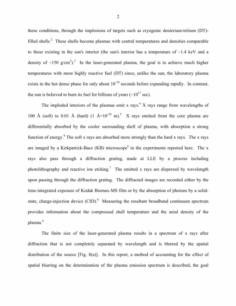
When the PCLC flakes are put into a cell they are suspended in a host fluid.
There are several highly desirable traits for this fluid to have. First, it must have the same
index of refraction as the PCLC flakes in use. Light is scattered at each interface
between materials with different indexes of refraction (figure 2.1). When trying to build
Figure 2.1- At each surface with a different index of refraction, light is scattered
a high-quality optic, scatter is a major problem. If light is scattered it is not transmitted
down the laser path, decreasing the efficiency of the entire system. In order to get a fluid
with the desired index of refraction and still be able to meet the other criteria necessary
for a host fluid, different liquids were mixed together. This allowed a mixture to be
produced with exactly the desired traits.
Second, the fluid should have the same density as the flakes. This will keep the
flakes suspended in solution, allowing an optic to be turned at any angle while still giving
6

Ryan Burakowski
consistent results. Having matching densities is ideal, but not absolutely necessary. If
the flakes have a different density than the fluid, they should align against one of the
substrates. This may be a useful technique for encouraging alignment. The drawback to
it would be that the optic could only be used in a perfectly horizontal position or with a
thinner than optimal cell gap to keep the flakes from moving. I made several mixtures of
fluids, some that had densities that matched the flakes and some that had different
densities, to explore the relationship between mismatched densities and flake alignment.
Since the host fluid is a mixture of its component liquids, it is essential that the
components are miscible with each other. To determine this, I conducted a series of
miscibility tests using the liquids I planned to use in my host fluids. I took mixtures of
liquids, put them into small bottles, and shook them. Only fluids that remained clear
when shaken were miscible and could be used as host fluids for the PCLC flakes.
The third important requirement for the host fluid is that it must be chemically
compatible with the flakes. Some fluids will dissolve the flakes, rendering them useless.
In order to test for chemical compatibility, I took samples of all the fluid mixtures that
met the previous standards and added a small amount of flakes to the fluids. The fluids
that were chemically compatible shimmered with the light being reflected off the flakes.
Since the angle of incidence partially determines the wavelength of light reflected, the
bottle of fluid and flakes shimmered with many colors and was very bright. When fluids
were not chemically compatible it was immediately obvious. When flakes were added
the fluid turned the dark, murky brown color of muddy water. The flakes dissolved into
the fluid and discolored it. Only solutions that shimmered with many colors could be
used as possible host fluids.
7

Ryan Burakowski
2.2 Concentration of PCLC Flakes
An LC optic will tend to reflect all the light of one handedness (50% of the total
for unpolarized incident light) at its selected wavelength while allowing all other
wavelengths of light to pass through. In order for PCLC flakes to achieve this goal, there
must be a large number of flakes that are all well-aligned in a cell. They must uniformly
cover the entire aperture of the optic to produce a uniform beam of reflected light. One
of the most important aspects of determining the viability of a PCLC circular polarizer is
getting enough flakes into the cell gap. No matter how well aligned they are, if there are
not enough flakes the device will not be efficient enough to be utilized. In order to test
how many flakes an optic can hold effectively under a given set of parameters, I built
small test cells to simulate the properties of an optic. I used microscope slides as
substrates, and cut them to about 2/3 of their original length to make the area in which I
had to align the flakes smaller. By mixing glass microspheres into UV epoxy, and then
adhering two slides together by putting dabs of epoxy at each of the four corners, I
created a test cell that had a uniform gap, the size of which depended upon the
microspheres used (figure 2.2). By holding every variable the same except for flake
Glass Substrate Host fluid PCLC Flake
Side View of Test Cell
Figure 2.2- Side view of a test cell. Microscope slides were used as the glass substrate.
8

Ryan Burakowski
concentration in the host fluid, I was able to make a series of test cells that showed the
relationship between concentration and maximum reflectance.
2.3 Alignment Techniques
The other important factor for determining the viability of a PCLC flake device is
how well the flakes can be aligned. If they are not all lined up in the same plane, the
flakes will target different wavelengths of light as the angle of incidence of the light
affects the wavelength of light that will be reflected. Several different methods to force
the PCLC flakes to align were tried. One was changing the characteristics of the host
fluid, namely its density. Another was using different methods to construct the test cell.
These methods should be able to be adapted to the construction of a full-size optic. By
keeping all the variables the same except for the alignment technique I was testing, I
developed cells to be used as controls and cells to experiment with alignment techniques.
By comparing these cells against one another, I was able to tell whether the technique
helped in flake alignment.
2.4 Cell Gap
The cell gap is a significant variable, but not directly related to the efficiency of
the optic. The amount of flakes that can be fit into an optic (concentration) and how well
they are aligned will ultimately determine whether PCLC-flake circular polarizers are
feasible. The gap between the two substrates is important because it directly affects both
the concentration limits of flakes in the host fluid and how well they are able to be
aligned. In order to determine the best possible size for the cell gap, I first had to find the
9

Ryan Burakowski
best way to align the flakes and what the optimum concentration of flakes was. Then,
using these parameters to build several test cells that were identical except for the gap
between the substrates, I was able to compare the results from these test cells and
determine the best possible size for the cell gap. The results from these experiments are
given in section 3.4.
2.5 Multi-wavelength Filters
Multi-wavelength filters are an extension of circular polarizers. When
constructed using low-molar-mass LC’s, multi-wavelength filters are circular polarizers
layered together into one larger optic. Each individual layer of LC reflects one
wavelength of light, and the multiple layers of different LC result in a multi-wavelength
circular polarizer. Because of the need to have layers of glass separating each type of
liquid crystal, there is a large amount of scatter and specular reflection in these optics.
PCLC flakes can theoretically make more efficient multi-wavelength filters.
Since different types of flakes that would reflect different wavelengths of light do not
react with each other, it should be possible to put multiple types of flakes into the same
cell gap. This type of optic would require much less glass than comparable low-molar-
mass LC filters, meaning there would be less unwanted reflections and less scatter (figure
2.3).
All the challenges of making a PCLC flake circular polarizer would be magnified
in a multi-wavelength filter. There would need to be a great amount of several different
types of flakes, and they would all have to be well-aligned. In essence, if a device is built
with two reflective wavelengths, the requirements in concentration and alignment for a
10

Ryan Burakowski
circular polarizer must be met twice over. The main goal of this project is to attempt to
prove a single-wavelength polarizer viable. Testing on multi-wavelength filters shows
that the scope of this project can be expanded upon.
Figure 2.3- A low-molar-mass liquid crystal multi-wavelength filter compared to a PCLC flake multi-wavelength filter. The PCLC flake filter uses much less glass, which is expensive and increases scatter.
3. Results
3.1 Host Fluid
Through the process described in section 2.1 I found a host fluid that matched all
the desired criteria. The calculations for determining the index of refraction and density
of a fluid made from two components are based upon a linear relationship to the percent
composition of each liquid. In the search for the right host fluid I conducted tests using
mixtures that included Bromonaphthaline, PDM-7050, propylene carbonate, DMS-T12,
Mistie, and DMS-T31. I found the ideal fluid in the form of a mixture of 10.7%
propylene carbonate and 89.3% PDM-7050. It had the same index of refraction, 1.57, as
the flakes I was using, was chemically compatible with the flakes, and the components
were miscible with each other. The density of the fluid was nearly ideal, too. The
11

Ryan Burakowski
density of the flakes I used was ~1.10 g/cm3, and the fluid’s density was calculated to be
1.101g/cm3.
3.2 Alignment Techniques
I tried several different techniques to align the PCLC flakes. The first was
manipulating the host fluid. By having a fluid with a density that was different from that
of the flakes, the flakes were forced to align against one of the substrates. An interesting
finding was that when the density of the fluid was greater than that of the flakes, forcing
them to rise to the surface, the cell reflected a higher percentage of light at its targeted
wavelength, yet when the density of the fluid was less than that of the flakes, allowing
them to sink to the bottom, the reflection at the targeted wavelength actually decreased.
By using a host fluid that had a density 0.1g/cm3 greater than that of the flakes, maximum
0.00%
5.00%
10.00%
15.00%
20.00%
25.00%
30.00%
35.00%
40.00%
-0.02 0 0.02 0.04 0.06 0.08 0.1 0.12
Difference in Density (Density of Fluid Minus Density of Flakes)
% R
efle
ctio
n
80 micron, Capillary fill, 5%flakes
Figure 3.1- Dependence of the reflectivity on the density of the host fluid relative to the PCLC flakes. All factors except for the density of the host fluid were held constant. The relationship is nearly linear.
12
Ryan Burakowski
reflection was increased substantially from 22.8% to 34.6% (figure 3.1). The 34.6%
reflectivity was the highest observed in any of the tests. This shows that a density
difference could be an extremely effective alignment technique if the optic it was applied
in could stay perfectly horizontal throughout its entire operating life. Since this is not the
case in the OMEGA laser system at the moment, I had to find another method for
aligning the PCLC flakes in my test cells.
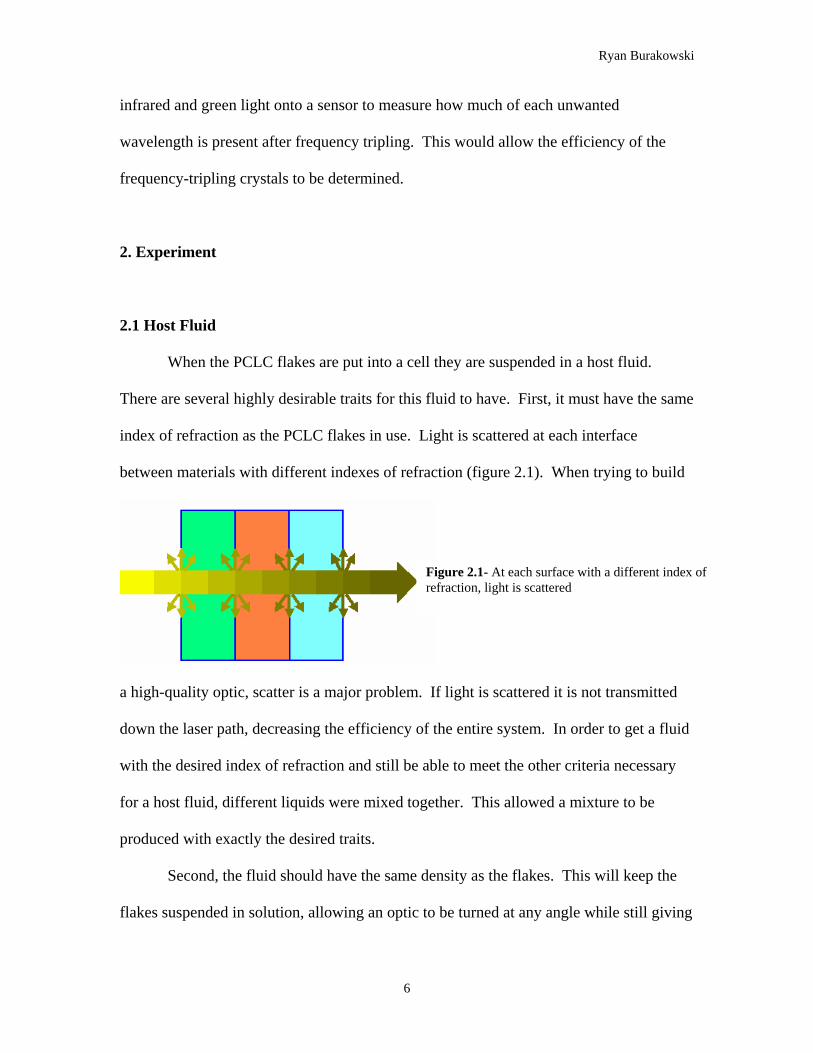
The other method I used in an attempt to improve alignment was to alter the way
the test cells were built. Traditionally, test cells were constructed by adhering the two
substrates together and then filling the gap with the PCLC flakes in their host fluid by
utilizing capillary action. I tried two new methods of construction of the cells. The first
method was to put the PCLC flakes in the host fluid on the bottom substrate, and then put
the top substrate on and shear the substrates against each other moving in the longer
direction of the microscope slides (figure 3.2). This improved upon the results from the
Figure 3.2- The shear method. Arrows show which way the top substrate slides over the bottom substrate.
capillary fill method used previously, increasing reflection from the previous maximum
of 22.8% to 28.5%. The second new construction method was the “twisting shear”
method. It also started with putting the PCLC material on the bottom substrate, but then
the top substrate was twisted back and forth across the bottom substrate (figure 3.3). This
improved reflection even more than the first shearing method I experimented with (figure
3.4), reaching a maximum reflection of 30.18% at a concentration of 7.5% flakes by
weight.
13
Ryan Burakowski
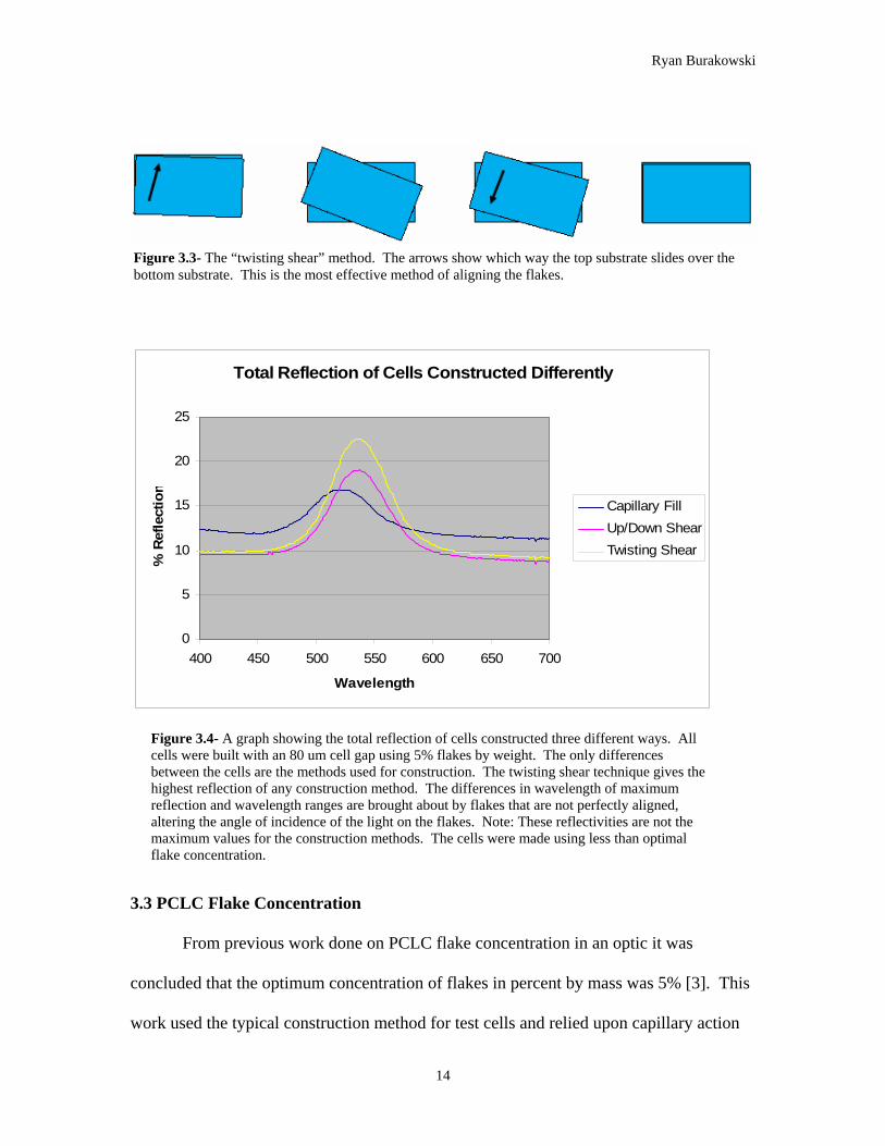
Figure 3.3- The “twisting shear” method. The arrows show which way the top substrate slides over the bottom substrate. This is the most effective method of aligning the flakes.
Total Reflection of Cells Constructed Differently
0
5
10
15
20
25
400 450 500 550 600 650 700
Wavelength
% R
efle
ctio
n
Capillary FillUp/Down ShearTwisting Shear
Figure 3.4- A graph showing the total reflection of cells constructed three different ways. All cells were built with an 80 um cell gap using 5% flakes by weight. The only differences between the cells are the methods used for construction. The twisting shear technique gives the highest reflection of any construction method. The differences in wavelength of maximum reflection and wavelength ranges are brought about by flakes that are not perfectly aligned, altering the angle of incidence of the light on the flakes. Note: These reflectivities are not the maximum values for the construction methods. The cells were made using less than optimal flake concentration.
3.3 PCLC Flake Concentration
From previous work done on PCLC flake concentration in an optic it was
concluded that the optimum concentration of flakes in percent by mass was 5% [3]. This
work used the typical construction method for test cells and relied upon capillary action
14

Ryan Burakowski
to fill the cell gap. With my new alignment technique of “twisting shear”, I was able to
bolster the optimum concentration to 7.5% flakes by weight, an increase of 50% over the
previous concentration achieved (figure 3.5).
0
5
10
15
20
25
30
35
0 2 4 6 8 10
wt% Flakes
% R
efle
ctio
n
12
Alignment TechniquesNo Alignment
Figure 3.5- A graph showing the reflectivity of cells vs. the concentration of flakes in percent by weight for cells in this study (aligned) and for previously made cells (not aligned). The alignment techniques drastically increased the amount of flakes that can be effectively inserted into a device, thereby increasing reflectivity. The optimum amount of flakes was increased from 5% by weight to 7.5% by weight.
3.4 Cell Gap
In initial experiments, when finding out the optimized concentration of PCLC
flakes in a test cell filled by capillary action, there was no variation in cell gap [3] [4]. It
was not known how changing the cell gap would affect the concentration and alignment
of flakes. Through my tests, regardless of what construction method was used, an 80 um
cell gap yielded the highest consistent reflectivities. The reflectivity of my test cells
drastically decreased when the cell gap decreased. The maximum reflection for a test
cell made with an 80 um cell gap was 30.18%, while the maximum for a 40 um cell gap
was only 22.49%. When the cell gap is increased to over 80 um, the reflectivity of the
cell varied randomly. This shows that the flakes have too much room to float around in
and are constantly changing their alignment. It seems that an 80 um cell gap allows for
15

Ryan Burakowski
the greatest number of flakes in the cell while keeping them well-aligned, yielding the
highest consistent reflectivities.
3.5 Multi-wavelength Filters
I made a two-color filter with flakes reflecting in the red and flakes reflecting in
the blue range. The reflectance measured by a spectrophotometer clearly showed two
peaks, one in the red wavelength range and one in the blue range (figure 3.6). This
proved that the concept of a multi-wavelength PCLC flake filter is viable. Using 5% by
mass of each kind of flake for a total of 10% flakes, I was able to reach a maximum of
22% reflection at each peak, while still letting the same amount of untargeted light
transmit through as in a single color PCLC circular polarizer. This is a very promising
area for future study.
Total Reflection for Cell026
0
5
10
15
20
25
400 459 518 577 636 695
Wavelength
% R
efle
ctio
n
Total Reflection
Figure 3.6- A graph showing reflectivity vs. wavelength in a two-color PCLC multi-wavelength filter.One PCLC flake type reflects light in the blue range and the other PCLC flake type reflects light in the red range. Notice the two distinct peaks in the graph. Each one represents the targeted wavelengths oone kind of PCLC flakes. Reflection went down to normal between the peaks, indicating that the two flake types did not interfere with each other.
f
Figure 3.6- A graph showing reflectivity vs. wavelength in a two-color PCLC multi-wavelength filter. One PCLC flake type reflects light in the blue range and the other PCLC flake type reflects light in the red range. Notice the two distinct peaks in the graph. Each one represents the targeted wavelengths of one kind of PCLC flakes. Reflection went down to normal levels between the peaks, indicating that the two flake types did not interfere with each other.
16

Ryan Burakowski
4. Conclusion/ Future Work
4.1 PCLC Circular Polarizers
The goal of this work was to determine the viability of a PCLC flake circular
polarizer. Even though significant advances were made in this work, it is likely that more
improvement will be made in the future. Previously, the maximum reflectivity achieved
with a PCLC-flake circular polarizer was 14.8%. Through the use of new construction
techniques that facilitated flake alignment and increased the maximum amount of flakes
that can be used in a cell, the reflectivity was increased to 30.18%, doubling the
effectiveness of these cells (figure 4.1). There is still room for improving the reflective
Total Reflection for Cell016
0
5
10
15
20
25
30
35
400 450 500 550 600 650 700
Wavelength
% R
efle
ctio
n
TotalReflection
Figure 4.1- The graph of reflectivity vs. wavelength for a cell constructed using the twisting sheamethod, an 80 um cell gap, and an ideal host fluid with 7.5% flakes by weight suspended in it. The maximum reflectivity I wa
r
s able to achieve was 30.18%. This is the highest reflectivity in this work that uses a density-matched fluid.
Figure 4.1- The graph of reflectivity vs. wavelength for a cell constructed using the twisting shear method, an 80 um cell gap, and an ideal host fluid with 7.5% flakes by weight suspended in it. The maximum reflectivity I was able to achieve was 30.18%. This is the highest reflectivity in this work that uses a density-matched fluid.
characteristics of these devices, such as using a UV curable polymer to lock well-aligned
flakes into place while using only one substrate or wetting the base substrate, sprinkling
17

Ryan Burakowski
hydrophobic flakes onto the wet glass, then allowing the water to dry, leaving the flakes
that had been on the surface of the water to lay flat on the substrate. With more
experimentation and new methods for the alignment of the PCLC flakes, it could well be
possible to use PCLC flake circular polarizers in the OMEGA laser system.
4.2 Multi-wavelength Filters
Multi-wavelength PCLC flake filters were tested to determine whether the theory
behind them can is valid. The concept was demonstrated through reflectivity
measurements taken on a test cell using multiple PCLC flakes that targeted different
wavelengths. The graph of reflectivity vs. wavelength plotted for a two-colored circular
polarizer clearly showed two distinct peaks characteristic of the selective reflection
properties of the two types of PCLC flakes. The two types of flakes in the cell did not
interfere with each other. Further work on this type of optic will be carried out to
evaluate its potential for use in diagnostics in the OMEGA laser system because of the
benefits that can be realized through this design.
5. Acknowledgments
First, I would like to thank Dr. R. Stephen Craxton for giving me the opportunity
to pursue this project. I would also like to thank my advisor, Dr. Tanya Z. Kosc, for all
the help she has willingly given me. Others who deserve special recognition are
Dr. Stephen Jacobs, Mr. Ken Marshall, Christopher Coon, and Katherine Hasman.
18

Ryan Burakowski
6. References
1) P.J. Collings and M. Hird, Introduction to Liquid Crystals: Chemistry and Physics
(Philadelphia, PA: Taylor and Francis, 1997).
2) E.M. Korenic, S.D. Jacobs, S.M. Faris, and L.Li, “Cholesteric liquid crystal
flakes-a new form of domain,” Mol. Cryst. Liq. Cryst. 317, 197-219_1998.
3) Kosc, Tanya Z., private communication.
4) Marshall, Ken, private communication.
19

Development of Polar Direct Drive Designs for Initial NIF Targets
Alexandra Cok

Development of Polar Direct Drive Designs for Initial NIF Targets
Alexandra M. Cok
Allendale Columbia School
Rochester, New York
Advisor: Dr. R. S. Craxton
Laboratory for Laser Energetics
University of Rochester
Rochester, New York
November 2006

Alexandra M. Cok
Abstract
This work proposes a means by which the National Ignition Facility (NIF) laser system,
being built for indirect-drive laser fusion, can be used for symmetric direct-drive implosions
producing high fusion neutron yields as soon as the NIF is operational. It uses polar direct drive
(PDD), which involves repointing the laser beams away from the center of the target in an
attempt to maintain shell radius uniformity during the implosion. All PDD designs proposed to
date need specially designed phase plates that will not be available for initial NIF experiments.
However, this work shows that good uniformity can still be obtained without special phase plates
by certain combinations of defocusing and pointing of the beams, including pointing offsets of
individual beams within the NIF laser beam quads, which are easy to implement. Two designs
have been developed using the two-dimensional hydrodynamic simulation code SAGE. The first
design uses the elliptical phase plates that will be used for indirect drive on the NIF; the second
design uses no phase plates. Both designs will make high-yield direct-drive implosions possible
with the initial NIF setup.
1. Introduction
Nuclear fusion provides a possible source of clean, abundant energy. One approach to
fusion uses laser beams to irradiate a spherical target containing fuel comprised of deuterium and
tritium, two isotopes of hydrogen, inside a shell of a material such as plastic or glass. The outside
of the shell ablates outwards and the inside is compressed inwards, compressing the fuel to high
densities and temperatures. The extreme temperature of the fuel overcomes the Coulomb
repulsion forces of the positively charged nuclei, and the extreme compression ensures a large
number of fusion reactions before the fuel explodes. The deuterium and tritium fuse to form a
helium nucleus, releasing an energetic neutron. Most of the energy released by fusion reactions is
2

Alexandra M. Cok
in the form of energetic neutrons. The energy of the helium nucleus is redeposited in the
compressed fuel if the density and radius of the fuel are great enough. This redeposition of
energy is known as ignition. Ignition is the first step to gaining breakeven, when the energy
released from fusion reactions exceeds that input by the laser. Laser fusion will not be a viable
source of abundant energy unless breakeven is achieved.
There are two different approaches to laser fusion: direct drive1 and indirect drive2. With
direct drive, laser beams hit the target pellet at normal incidence from all directions [Figure 1(a)].
This is the type of fusion for which the OMEGA laser system at the University of Rochester's
Laboratory for Laser Energetics is configured. With indirect drive, the target pellet is surrounded
by a “hohlraum”, a cylinder made of gold or another material with a large atomic number [Figure
1(b)]. Laser beams enter the hohlraum through openings cut into the top and bottom. When hit
by the laser beams, the hohlraum emits x rays, which then irradiate the target pellet, providing
the energy needed for compression. Almost all of the initial laser energy is absorbed by the gold
and close to 80% is reemitted as x rays. However, only 20% is actually absorbed by the target
pellet; the rest is absorbed by the walls of the hohlraum or lost through the openings in the
hohlraum. The lower energy efficiency of indirect drive is made up for by the greater uniformity
of x ray radiation of the target. The National Ignition Facility (NIF), currently being constructed
at Lawrence Livermore National Laboratory, will be configured for indirect drive.
Figure 1. The two main approaches to laserfusion. (a) In direct drive, the laser beamsirradiate the target pellet. Arrows representlaser beams and the dotted circle shows howthe shell implodes. (b) In indirect drive, thetarget pellet is contained in a cylindricalhohlraum, which is hit by lasers enteringthrough holes in the top and bottom of thehohlraum. The hohlraum produces x rays(open arrows), which irradiate the target.(a) Direct Drive (b) Indirect Drive
3

Alexandra M. Cok
The NIF is due for completion in 2010, at which point it will become the world’s most
powerful laser. The NIF has 192 beams designed to deliver a total of 1.8 MJ of energy to the
target, theoretically enough energy to achieve ignition and breakeven. The NIF laser beams are
incident from the top and bottom of the target pellet. The laser beam ports are arranged in four
rings at angles of 23.5°, 30.0°, 44.5°, and 50.0° from the vertical in the upper hemisphere with
four corresponding rings in the lower hemisphere. There are a total of 48 ports; laser beams are
arranged in groups of four called quads, so there is one quad per port. Each beam is square,
measuring 40 cm by 40 cm. Symmetric direct-drive experiments, with a configuration similar to
that shown in Figure 1(a), are not planned until around 2016, as this will involve repositioning
half of the beams to another ring at 77.45°, an expensive and time-consuming process. A scheme
termed polar direct drive (PDD)3 has been proposed to enable earlier direct-drive experiments on
the NIF. If the indirect-drive beams are simply aimed at the center of the target, as in Figure 2(a),
the target shell receives significantly more drive on the poles than on the equator. As a result, the
ratio of the shell velocity at the poles to the shell velocity at the equator is approximately two to
one. Such distortion in the shell is not acceptable since shell radius uniformity is necessary to
obtain high compression. The proposed PDD solution to this is to repoint the beams away from
the center of the target, minimizing the differences in the amount of drive on all portions of the
target shell [Figure 2(b)].
Figure 2. The possible ways in which theNIF laser beams, positioned for indirectdrive, can irradiate a direct-drive target.(a) When the laser beams are aimed at thetarget center, the shell implodesnonuniformly. (b) Polar direct drive, inwhich the beams are repointed away fromthe center of the target, causes a nearlyuniform implosion. Rings 1-4 areindicated in (a).
34
43
2 1
2 1(a) (b)
Prior to producing the energy required for ignition experiments (1.0 to 1.8 MJ), the NIF
4

Alexandra M. Cok
laser system and diagnostic systems will be tested at an energy of 375 kJ to ensure that the laser
optics are not damaged. In particular, the neutron diagnostic systems must be tested. Direct-drive
fusion must be used to obtain the maximum number of neutrons at this energy, because at low
energies indirect drive cannot provide sufficiently high temperatures and compression to yield as
large a number of neutrons. Therefore, PDD designs maximizing the shell radius uniformity
must be developed.
All previous PDD designs3-6 required special phase plates (see Section 2.2 below).
Unfortunately, these will not be available initially on the NIF. This work has investigated
alternate ways of developing PDD designs, involving certain combinations of beam defocusing
and pointing that are straightforward to implement. This work has resulted in two designs that
will make the desired initial experiments possible.
2. Parameters Available for Optimization
The key parameters available for developing the two-dimensional designs are
specifications for shifting the beam pointings away from the center of the target and defocusing
the beams (Section 2.1). The optimum combinations of shifting and defocusing depend on the
availability of indirect-drive phase plates (Section 2.2). Section 2.3 describes “split quads” in
which the four beams are shifted slightly differently so that they do not overlap exactly.
2.1 Shifting and Defocusing
Figure 3(a) shows the important optics near the end of the laser system that control the
parameters described here. The beam pointing is shifted away from the center of the target by
moving the mirror. The center of the beam then moves a specified distance in the direction
perpendicular to its axis, so that the beam hits the target at a different spot [Figure 3(b)].
Defocusing the beam is done by moving the focus lens toward the target. The laser beam
5

Alexandra M. Cok
spot on the target is then enlarged and the maximum intensity decreases. To gain the best
uniformity and overlap of laser beams, the diameter of the beam spot should generally
correspond to the diameter of the target shell. Defocusing can be used to change the relative
intensities of the four rings of beams as well as to change the size of each beam spot.
(a) (b) (c)igure 3. (a) Diagram (not to scale) showing the parts of the laser that control the parameters used in this
amplification optics. These irregularities, if uncorrected, will imprint as hot spots on the target
a more uniform beam after focusing. Different types of phase plates are used to produce different
sizes of beam spots. For direct drive, the beam spots need to be large to cover the target. For
indirect drive, the beams need to be small enough to pass through the openings in the hohlraum
without hitting the edges of the openings and generating plasmas (see Figure 4). Such plasmas
would cause the laser beam rays to refract and strike the hohlraum wall in the wrong place or
even prevent the rays from entering the hohlraum. The NIF will have two different types of
phase plates: those for inner beams (rings one and two, see Figure 4) and those for outer beams
z
y
40 cm
Shift
Target
2 mm7 m
MirrorPhase PlateLens
2 mm Target 40 cm
Best Focus
Defocus
2.2 Phase Plates
Laser beams accumulate small irregularities in coherence after passing through the many
e gement of four beams in a quad at the output of the laser system.
Fwork. Moving the lens along the beam axis controls the size of the beam at the target and tipping the mirrorcontrols beam pointing. (b) Diagram showing how beam ring shifts are measured perpendicular to thebeam direction. The angle of the beam from the vertical remains virtually constant. (c) Diagram showingth arran
affecting the uniformity of the implosion. Phase plates7,8 are special optics through which the
beams pass before they are focused. A phase plate spreads the energy of the beam slightly to give
6

Alexandra M. Cok
(rings three and four). The phase plates that will be used on the NIF will produce small elliptical
focal spots because of the angles at which the beams enter the hohlraum (see Figure 4). The size
of the spot depends on the angle at which the beams pass through the openings in the hohlraum.
Therefore, since the beams in rings three and four enter at much shallower angles, their spot sizes
must be smaller than those produced for rings one and two. The small spot sizes produced by the
NIF indirect-drive phase plates make them unsuitable for direct-drive experiments unless the
beams are defocused. The development of two PDD designs in this work, one with phase plates
and one without, allows for flexibility depending on the availability of the NIF indirect-drive
phase plates.
Figure 5 shows a comparison of beams in best focus and beam
Figure 4. The proposed indirect drivepointings for the NIF. From each end,beams are aimed at two verticalpositions on the hohlraum wall. Rings 1and 2 (the inner beams) are aimed atone position and rings 3 and 4 (theouter beams) are aimed at another. Inorder for the beams to be able to fitthrough the openings in the hohlraum,they must be circular as they pass intothe hohlraum. Therefore, the beamshave elliptical cross sections. The outerbeams have semi-axes (a, b1) and theinner beams have semi-axes of (a, b2).Because of the greater angle, the outerbeams are much more elliptical thanthe inner beams.
Inner beams (θ=23.5°, 30°) Outer beams
(θ=44.5°, 50°)
2a 2b1
2b2
s out of focus, with and
without phase plates. Figure 5(a) shows the intensity contours of a small ring-four best-focus
spot without a phase plate, whose size is determined by the optical aberrations in the laser. Each
contour represents a 10% increase in intensity, starting at 10% of peak intensity. Figure 5(b)
shows a ring four beam in best focus with a phase plate. Figures 5(c) and (d) show the intensity
7

Alexandra M. Cok
contours of a ring-four beam out of focus (defocused by 1.7 cm) with and without a phase plate.
Without a phase plate, the best-focus spot is round. As the beam is taken farther out of best
focus, the spot becomes increasingly square, corresponding to the square beam shape at the
output of the laser.
300 µm
1100 µm
1200 µm
1700 µm
1.7 cm. Each contour represents a 10% increase in intensity starting with 10%.
Figure 5. (a) The intensity contour plot of a ring 4 beam in best focus. (b) The intensity plot of a ring 4 plate in best focus. (c) A ring 4 beam without a phase plate, out of best focus with a.7 cm. (d) A ring 4 beam with a phase plate, out of best focus with a defocus distance
beam with a phasedefocus distance 1
2.
ar
as
fo
Q
is
(a) No phase plate, best focus (b) Phase plate, best focus
(c) No phase plate, defocused (d) Phase plate, defocused
3 Split Quads
The four beams of each quad, arranged at the output of the laser as shown in Figure 3(c),
e usually focused down to a single focal spot. However, as each beam has an adjustable mirror,
shown in Figure 3(a), it is possible to adjust the pointings of the four beams so that they are
cused to slightly different spots. This changes the overall shape of the intensity contours.
uads with pointings altered in this way will be referred to as “split quads.” Using split quads, it
possible to alter the shape of the beams from the elliptical spots created by the phase plates and
8

Alexandra M. Cok
to alter the rate at which the intensity of the beam drops off away from the center of the beam.
Intensity contour plots of ring four beams using split quads are shown in Figure 6. These
beams are the same as those shown in Figure 5, except that in Figure 6 the beams have split
quads. In Figures 6(a) and (b) each beam is in best focus with and without a phase plate. In
Figure 6(c) and (d) each beam is out of focus (defocused by 1.7 cm). Figures 6(c) and (d) also
show the actual ring-four beam profiles used in the designs described later in this report. The rate
at which the intensity of the beam drops off away from the center of the beam is much less steep
when using a split quad [compare Figures 5(c) and 5(d) to Figures 6(c) and 6(d)]. The difference
is especially notable when not using a phase plate. By using a combination of split quad shifti
9
ng
and defocusing, the NIF beams can be enlarged by a factor of two or even more if necessary.(a) No phase plate, best focus (b) Phase plate, best focus
(c) No phase plate, defocused (d) Phase plate, defocused
1300 µm
∆y = 458 µm
∆z = 283 µm
300 µm
Figure 6. As in Figure 5, but each beam uses a split quad with shifts (
1700 µm
2000 µm
∆z, ∆y) = (283 µm, 458 µm) in (a) and (c) and (∆z, ∆y) = (247 µm, 155 µm) in (b) and (d). (c) and (d) show the intensity contours of the ring 4 beams actually used in the designs discussed later in this report.
Alexandra M. Cok
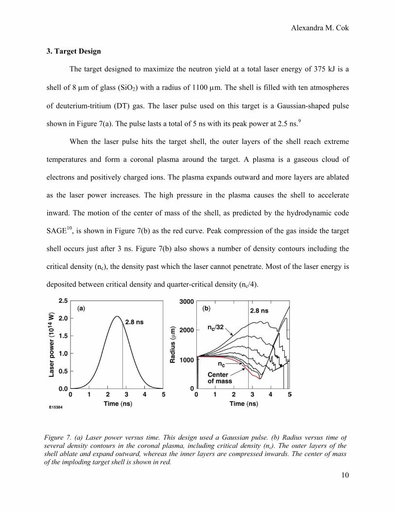
3. Target Design
The target designed to maximize the neutron yield at a total laser energy of 375 kJ is a
shell of 8 µm of glass (SiO2) with a radius of 1100 µm. The shell is filled with ten atmospheres
of deuterium-tritium (DT) gas. The laser pulse used on this target is a Gaussian-shaped pulse
shown in Figure 7(a). The pulse lasts a total of 5 ns with its peak power at 2.5 ns.9
When the laser pulse hits the target shell, the outer layers of the shell reach extreme
temperatures and form a coronal plasma around the target. A plasma is a gaseous cloud of
electrons and positively charged ions. The plasma expands outward and more layers are ablated
as the laser power increases. The high pressure in the plasma causes the shell to accelerate
inward. The motion of the center of mass of the shell, as predicted by the hydrodynamic code
SAGE10, is shown in Figure 7(b) as the red curve. Peak compression of the gas inside the target
shell occurs just after 3 ns. Figure 7(b) also shows a number of density contours including the
critical density (nc), the density past which the laser cannot penetrate. Most of the laser energy is
deposited between critical density and quarter-critical density (nc/4).
Figure 7. (a) Laser power versus time. This design used a Gaussian pulse. (b) Radius versus time ofseveral density contours in the coronal plasma, including critical density (nc). The outer layers of theshell ablate and expand outward, whereas the inner layers are compressed inwards. The center of massof the imploding target shell is shown in red.
10

Alexandra M. Cok
The implosion of the shell and the creation of a coronal plasma are shown in Figure 8. In
Figure 8(a), a raytrace plot of the shell is shown near the start of the laser pulse when the shell is
close to its starting position. The red lines represent the incoming rays from a ring-four laser
beam. The black contours are density contours, and the green region shows the position of the
shell. Figure 8(b) shows the shell at 2.8 ns, over halfway into the laser pulse. This plot shows the
implosion of the optimum design with phase plates. The two plots provide a comparison between
the starting shell and the shell when it has imploded halfway, and show that the shell has
maintained its uniformity through 2.8 ns.
Figtheco
(a) At 1.0 ns (b) At 2.8 ns
DT gas
Dist
ance
(µm
)
8 µm SiO2 nc/8
nc
ure 8. (a) A raytrace plot at 1.0 ns, near the start of the laser pulse. (b) A raytrace plot at 2.8 ns, when shell (green) has imploded halfway. These plots show representative rays of ring 4 and some density
ntours. The design used for this simulation was the design with phase plates.
11

Alexandra M. Cok
The importance of optimizing the designs is shown in Figure 9. In Figure 9(a), all of the
beams are pointed to the center of the target and the defocus is 3.5 cm for all of the beams. The
distortion in the shell at 2.8 ns is obvious as the shell forms an ellipse with semi-axes of 400 µm
and 750 µm. The ratio of velocities between the poles and the equator is 1.7 to 1 at 2.8 ns. Figure
9(b) shows the optimum design without phase plates at the same time. Raytrace plots such as
Figures 8 and 9 show where each ring of beams hits the target, how well the shell maintains
uniformity as it implodes, and where distortions in the shell occur.
Dist
ance
(µm
)
nc
Fhiu
(a) (b)
Ring 4
nc
Ring 4
igure 9. A comparison of two SAGE raytrace plots at 2.8 ns. (a) shows the implosion when the designas not been optimized, with all beams pointed to the center of the target. There is significant distortionn the shell. (b) shows the implosion when the design is highly optimized, and the shell maintains itsniformity. The optimized design used for (b) was the design without phase plates.
12

Alexandra M. Cok
The two optimum designs, illustrated in Figures 8(b) and 9(b), were developed after
numerous simulations using SAGE. SAGE provides parameters enabling the user to adjust the
beam profiles. Although the accuracy to which SAGE calculates the out-of-focus beam profiles
for NIF beams has not yet been experimentally determined, SAGE has accurately predicted the
out-of-focus beam profiles for OMEGA beams. Figure 10 shows experimental data for the
intensity of an OMEGA beam as a function of radius for best focus and two different defocus
distances (5 mm and 10 mm). The theoretical calculations obtained from SAGE are plotted with
the experimental data. The best focus was fit to a Gaussian of order n=7 [I∝exp-(r/r0)n with
r0=380 µm], from which SAGE calculated the out-of-focus beam profiles. The accuracy to which
SAGE calculates the out-of-focus profiles is excellent. It is reasonable to assume that SAGE will
4. Optimization Process and the Optimized Designs
calculate the out-of-focus profiles of NIF beams to a similar degree of accuracy.
elop the design that would cause the shell
imp
Figure 10. Graphs of intensityversus radius of an OMEGA beam atbest focus (z=0) and for two defocusdistances (z=5 mm and 10 mm). Thesolid lines correspond toexperimental data and the dashedlines correspond to SAGEsimulations.
The goal of the optimization process was to dev
to lode with the greatest degree of uniformity. Specifically, a design was sought that
produced the lowest deviation of shell radius at a late time into the pulse (2.8 ns), just before the
time of peak compression (see Figure 7). The optimization process involved running and
13
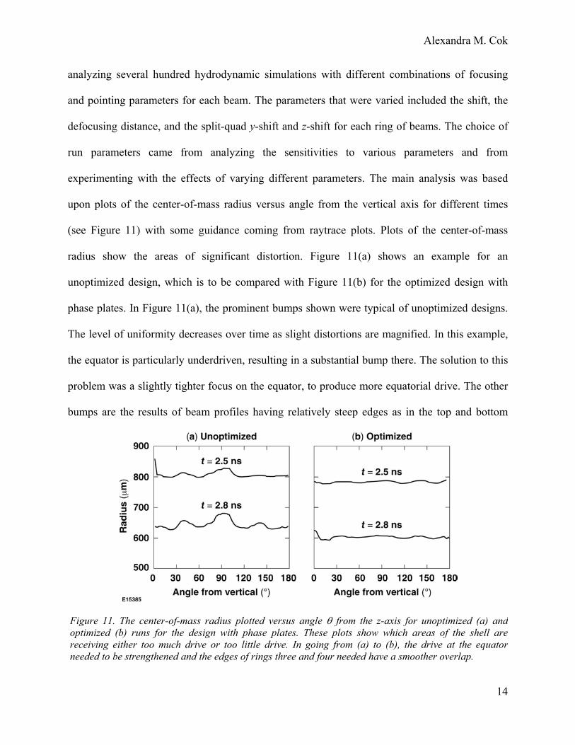
Alexandra M. Cok
analyzing several hundred hydrodynamic simulations with different combinations of focusing
and pointing parameters for each beam. The parameters that were varied included the shift, the
defocusing distance, and the split-quad y-shift and z-shift for each ring of beams. The choice of
run parameters came from analyzing the sensitivities to various parameters and from
experimenting with the effects of varying different parameters. The main analysis was based
upon plots of the center-of-mass radius versus angle from the vertical axis for different times
(see Figure 11) with some guidance coming from raytrace plots. Plots of the center-of-mass
radius show the areas of significant distortion. Figure 11(a) shows an example for an
unoptimized design, which is to be compared with Figure 11(b) for the optimized design with
phase plates. In Figure 11(a), the prominent bumps shown were typical of unoptimized designs.
The level of uniformity decreases over time as slight distortions are magnified. In this example,
the equator is particularly underdriven, resulting in a substantial bump there. The solution to this
problem was a slightly tighter focus on the equator, to produce more equatorial drive. The other
bumps are the results of beam profiles having relatively steep edges as in the top and bottom
Figure 11. The center-of-mass radius plotted versus angle θ from the z-axis for unoptimized (a) andoptimized (b) runs for the design with phase plates. These plots show which areas of the shell arereceiving either too much drive or too little drive. In going from (a) to (b), the drive at the equatorneeded to be strengthened and the edges of rings three and four needed have a smoother overlap.
14

Alexandra M. Cok
portions of Figure 5(d). When the edges of beams are steep, it is difficult to obtain equal amounts
of drive at angles where the beams overlap. The solution to this was to increase the split-quad ∆z
shift on rings three and four slightly. Also, the simulation code sometimes produced some
numerical noise such as the false peaks at θ=0° at 2.5 ns in Figure 11(a) and at 2.8 ns in Figure
11(b), but these were easy to identify and did not affect the overall optimization process. Overall
the simulations showed consistent behavior as laser parameters were varied.
The final set of parameters for the design with phase plates are shown in Table 1; the
aramep ters for the design without phase plates are in Table 2. These tables contain all the
specifications needed to implement these designs on the NIF. Parameters of particular interest
are the defocus distances and the split-quad shifts. As is evident, the defocus distance varies for
the four rings, with the smallest defocus distance on ring four. This is to provide the extra drive
needed at the equator by increasing the intensity of those beams. In the design with phase plates,
split quads are used on rings three and four. For ring four, this smoothes out the steeper drop-off
of intensity that would otherwise be present from the smaller defocus [compare Figures 5(d) and
6(d)]. The parameters for the design without phase plates are very similar, with the exception of
the split quads. For this design, rings two, three, and four all require split quads. Without phase
plates to spread the beam energy, the intensity drops off very quickly at the edge of the beam.
For the design without phase plates, the split quad shifts are significantly larger than for the
previous design. This provides the needed shift to alter the steep drop-off in beam intensity to a
more gradual rate of decrease of intensity. The more gradual rate of decrease makes it easier to
overlap the individual beams to provide the most uniform irradiation of the target.
15

Alexandra M. Cok
Angle
Pointing
Shift
Defocus
Distance
Phase Plate Split Quad
Z-Shift
Split Quad
Y-Shift
Ring 1 23.5° 50 µm 3.0 cm Inner ---- ----
Ring 2 30.0° 159 µm 3.5 cm Inner ---- ----
Ring 3 44.5° 250 µm 3.5 cm Outer 212 µm 141 µm
Ring 4 50.0° 494 µm 1.7 cm Outer 247 µm 155 µm
Table 2. Beam parameter specifications for the optimum design without phase plates.
p
t
p
6
T
d
m
o
e
d
f
Table 1. Beam parameter specifications for the optimum design using indirect-drive phase plates.
Both of these designs produced excellent shell radius uniformity. The design using phase
lates had a root-mean-square deviation of radius (∆Rrms) of approximately 4 µm at 2.8 ns, when
he shell has imploded to a radius of 600 µm, half of its initial radius. The design without phase
lates performed nearly as well, giving a root-mean-square deviation of radius of approximately
µm at the same time. Uniformity of velocity is also necessary to produce good compression.
hese designs produce uniformity of velocity to approximately 2% (rms) for the phase plate
esign and 4% (rms) for the design without phase plates.
Angle Pointing Shift Defocus Distance
Split Quad Z-Shift
Split Quad Y-Shift
Ring 1 23.5° 53 µm 3.0 cm ---- ---- Ring 2 30.0° 165 µm 3.5 cm 283 µm 458 µm Ring 3 44.5° 250 µm 3.5 cm 283 m 458 µm Ring 4 50.0° 494 µm 1.7 cm 283 µm 458 µm
The sensitivity of the designs to pointing errors has been explored. Ring four is the ring
ost sensitive to pointing errors because of the tighter focusing. The sensitivity to mispointings
f this ring is shown in Figure 12 for the two designs. These plots show the ∆Rrms of pointing
rror in the worst case scenario, where all of the ring 4 beams are mispointed in the same
irection. The values on the x-axis are the pointing errors relative to the optimum shift for ring
our (494 µm). Some short-scale structure resulting from numerical noise in the simulations is
16

Alexandra M. Cok
apparent very close to the optimum pointings. However, the graphs clearly show only a slight
reduction of uniformity for errors in the ±50 µm range. The NIF pointing specification is 50 µm
and pointings accurate to within 30 µm have been demonstrated11. Therefore, the pointing on the
NIF is more than adequate to produce good uniformity using these designs.
Figure 12. Sensitivity of the rms radius deviation at 2.8 ns to pointing errors of ring four from the optimum design in (a) the design with phase plates and (b) the design without phase plates.
5. Conclusion
Two experimental designs, including beam focus and pointing parameters, have been
developed using hydrodynamic simulations to provide optimal implosion uniformity for directly-
driven DT-gas-filled glass shells on the NIF. The development of these two designs makes it
possible to carry out spherical implosions on the NIF as soon as all 192 beams are operational. In
particular, high-neutron-yield implosions are possible on the NIF before the NIF is ready for
ignition experiments. The availability of both a design using the NIF indirect-drive phase plates
and a design using no phase plates allows for more flexibility according to what is available on
the NIF at the time. These designs are necessary for initial experiments to test the NIF neutron
diagnostic systems and will also enable direct-drive implosion experiments to be carried out
much sooner than would otherwise be possible.
17
Alexandra M. Cok
6. References
1. J. Nuckolls et al., “Laser Compression of Matter to Super-High Densities: Thermonuclear
(CTR) Applications,” Nature 239, 139 (1972).
2. J. D. Lindl, “Development of the Indirect-Drive Approach to Inertial Confinement Fusion
and the Target Basis for Ignition and Gain,” Phys. Plasmas 2, 3933 (1995).
3. S. Skupsky et al., “Polar Direct Drive on the National Ignition Facility,” Phys. Plasmas
11, 2763 (2004).
4. R. S. Craxton et al., “Polar Direct Drive: Proof-of-Principle Experiments on OMEGA
and Prospects for Ignition on the National Ignition Facility,” Phys. Plasmas 12, 056304
(2005).
5. J. A. Marozas et al., “Polar-Direct-Drive Simulations and Experiments,” Phys. Plasmas
13, 056311 (2006).
6. R. S. Craxton and D. W. Jacob-Perkins, “The Saturn Target for Polar Direct Drive on the
National Ignition Facility,” Phys. Rev. Lett. 94, 095002 (2005).
7. Y. Kato et al., “Random Phasing of High-Power Lasers for Uniform Target Acceleration
and Plasma Instability Suppression,” Phys. Rev. Lett. 53, 1057 (1984).
8. T. J. Kessler et al., “Phase Conversion of Lasers with Low-Loss Distributed Phase
Plates,” in Laser Coherence Control: Technology and Applications, edited by H. T.
Powell and T. J. Kessler (SPIE, Bellingham, WA, 1993), Vol. 1870, p. 95.
9. P. W. McKenty, Laboratory for Laser Energetics, private communication (2006).
10. R. S. Craxton and R. L. McCrory, “Hydrodynamics of Thermal Self-Focusing in Laser
Plasmas,” J. Appl. Physics. 56, 108 (1984).
11. R. A. Zacharias et al., “National Ignition Facility Alignment and Wavefront Control,” in
18

Alexandra M. Cok
Optical Engineering at the Lawrence Livermore National Laboratory II: The National
Ignition Facility, edited by M. A. Lane and C. R. Wuest (SPIE, Bellingham, WA, 2004).
Vol. 5341, p. 168.
19

Improved Laser Damage Resistance of Multi-Layer Diffraction Gratings
Vapor-Treated with Organosilanes
Zuzana Culakova

Zuzana Culakova
Improved Laser Damage Resistance of Multi-Layer Diffraction Gratings
Vapor-Treated with Organosilanes
Zuzana Culakova
Brighton High School Rochester NY, 14618
Advisor: Kenneth L. Marshall
Laboratory for Laser Energetics University of Rochester
Rochester, NY August 2006

Zuzana Culakova
Abstract
Multi-layer dielectric gratings are used in high power laser systems to compress
laser energy pulses. The final power of these short pulse petawatt class systems is limited
by the laser damage resistance of the optical components in the system, especially the
diffraction gratings. This work was motivated by the previous discovery that vapor-
treatment of gratings with hexamethyldisilazane (HMDS) can increase the damage
threshold. Gratings were laser damage tested, and then a simple room temperature vapor-
deposition technique was used to coat them with several different disilazane compounds.
The gratings were then damage tested again to determine if an increase in damage
threshold had occurred. The laser-induced damage threshold of an HMDS-treated grating
increased by 4.5% in a 1-on-1 damage test, while that of a tetramethyldisilazane-treated
grating increased by 16.5% in an N-on-1 damage test. Both the N-on-1 and 1-on-1
damage thresholds of a bis-(trifluoropropyl)tetramethyldisilazane-treated grating
increased, by 4.8% and 5.3 % respectively. Such increases in laser damage threshold are
unprecedented and counterintuitive because it is widely accepted that the presence of
organic material or coatings on the surfaces of optical substrates decreases their laser
damage resistance. The results are especially encouraging since they were obtained on
samples of sub-optimal quality. The next logical step is to attempt to confirm this effect
on high-quality, freshly cleaned grating samples.
1. Introduction
High energy petawatt (HEPW) laser systems are capable of producing beams of
unprecedented intensities for high energy density physics experiments. In a number of
2

Zuzana Culakova
countries around the world, these systems are being built to develop laser fusion as an
alternate energy source. Laser fusion uses lasers to compress and heat targets containing
hydrogen isotopes, initiating fusion - the combination of nuclei to form helium and
energetic neutrons. The current goal of laser fusion research is to reach and exceed
“break even”- the point at which the amount of fusion energy produced equals the energy
consumed by the laser. Two HEPW systems, Japan’s GEKKO Petawatt and the United
Kingdom’s Vulcan Petawatt are currently in operation, while several more, including the
OMEGA Extended Performance (EP) laser, are under construction or in planning1.
OMEGA EP is an addition to the existing fusion laser system, OMEGA, at the
University of Rochester Laboratory for Laser Energetics (LLE). The OMEGA EP
system, expected to begin operation in 2008, will have two beamlines equipped with a
short pulse (1 ps to 100 ps) capability at a wavelength of 1053 nm. These two beams can
be directed into the OMEGA laser’s target chamber to be used for fast ignition
experiments, which use a pulse of energetic electrons to heat the compressed fuel, thus
igniting the fusion reaction2, and to produce short pulses of x rays to “backlight”
imploding fusion targets for diagnostic purposes. The short-pulse beams interacting with
plasmas produced by longer pulses will also be used to study high energy density
physics, such as high-intensity laser-matter interactions, in OMEGA EP’s target
chamber3,4.
The short pulses are created by chirped pulse amplification (CPA)5, as shown in
Figure 1. To amplify the laser pulse without damaging the amplifier, a short pulse from
the source is first chirped, or stretched into a longer, lower-power pulse in which the
longer wavelengths travel at the front. The pulse is amplified and then compressed by a
3
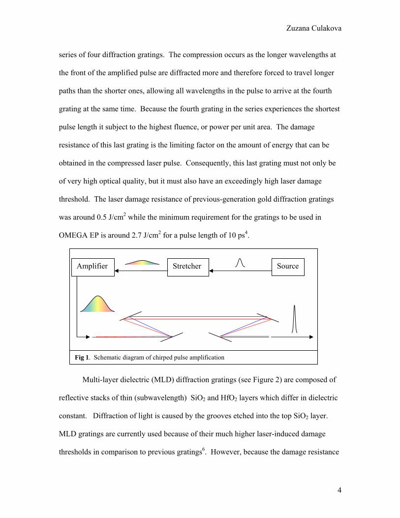
Zuzana Culakova
series of four diffraction gratings. The compression occurs as the longer wavelengths at
the front of the amplified pulse are diffracted more and therefore forced to travel longer
paths than the shorter ones, allowing all wavelengths in the pulse to arrive at the fourth
grating at the same time. Because the fourth grating in the series experiences the shortest
pulse length it subject to the highest fluence, or power per unit area. The damage
resistance of this last grating is the limiting factor on the amount of energy that can be
obtained in the compressed laser pulse. Consequently, this last grating must not only be
of very high optical quality, but it must also have an exceedingly high laser damage
threshold. The laser damage resistance of previous-generation gold diffraction gratings
was around 0.5 J/cm2 while the minimum requirement for the gratings to be used in
OMEGA EP is around 2.7 J/cm2 for a pulse length of 10 ps4.
Stretcher Amplifier Source
Fig 1. Schematic diagram of chirped pulse amplification
Multi-layer dielectric (MLD) diffraction gratings (see Figure 2) are composed of
reflective stacks of thin (subwavelength) SiO2 and HfO2 layers which differ in dielectric
constant. Diffraction of light is caused by the grooves etched into the top SiO2 layer.
MLD gratings are currently used because of their much higher laser-induced damage
thresholds in comparison to previous gratings6. However, because the damage resistance
4

Zuzana Culakova
of the last grating is the limiting factor on
the energy of the laser, new ways to
increase the damage threshold are
desirable.
Fig 2. SEM micrograph of an MLD grating. The grooves are 500 nm deep.
In preliminary experiments by the
Optics and Imaging Sciences group at
LLE, gratings were exposed overnight to
the organosilane compound
hexamethyldisilazane, (HMDS), which is used in the semiconductor industry as a
coupling agent to increase the adhesion between a silica wafer and a photoresist.
Organosilanes are compounds composed of silicon atoms carrying up to four different
carbon-containing functional groups. MLD gratings that were vapor treated with HMDS
reproducibly demonstrated increases of >20% in laser damage thresholds7. This increase
in damage resistance, known as “laser hardening,” was unexpected and counterintuitive,
because conventional wisdom dictates that the presence of organic materials on optical
components will lead to reduced laser damage thresholds. The goal of this investigation
was to assess the reproducibility of the phenomenon, find the necessary conditions for the
reaction, and identify whether the laser hardening effect is unique to HMDS.
During this investigation, candidate organosilanes were used to vapor treat glass
slides to assess their potential for treating diffraction gratings. The chemistry of the
reaction of the compounds with silica surfaces is described in Section 2. Estimates of the
necessary exposure time for a saturated coating were obtained by measuring the water
contact angle on the surfaces, as summarized in Sections 3 and 4. Diffraction grating
5

Zuzana Culakova
samples were damage tested before and after treatment with the most promising
organosilanes, as described in Section 5. Section 6 details improvements in the laser-
induced damage thresholds that were found as a result of this treatment.
2. Chemistry of Organosilanes
Two different classes of organosilanes that bond easily to silica surfaces were
identified. Both disilazane (silamine) and chlorosilane compounds are widely used to
change the surface chemistry of silica capillary columns for gas chromatography by
bonding organic functional groups with widely different polarities to the inner surface of
the column8. Silylation occurs as the compounds react with and replace hydroxyl groups
on the silica surface. The reaction utilizes the natural vapor pressure of the chemicals and
proceeds in the vapor phase at room temperature and pressure. This feature makes vapor
treatment with these chemicals simple, and because it does not require heat, it avoids the
risk of shattering the sensitive MLD gratings by thermal shock. The disilazane
compounds can react completely in a two-step mechanism with the surface silanols (see
Figure 3). In this example, the HMDS first reacts with a surface hydroxide group to
attach one trimethylsilane group to the substrate surface to form trimethylaminosilane,
which further reacts with the surface to deposit a second trimethylsilane group, which
forms ammonia as a byproduct. The overall reaction with HMDS can be written as9:
2 ≡Si–OH + (CH3)3–Si–NH–Si– (CH3)3 → 2 ≡Si–O–Si(CH3)3 + NH3 (1)
6

Zuzana Culakova
The chlorosilane compounds react via a simpler single step reaction shown in Figure 4.
For example, a trimethylchlorosilane (TMCS) molecule interacts with the surface silanols
to deposit a single trimethylsilane group, forming hydrogen chloride gas as a byproduct
as shown in the equation below10:
≡Si–OH + (CH3)3SiCl → ≡Si–O–Si(CH3)3 + HCl (2)
SiO2 Surface Si Si Si Si Si
O OH
Si
O O Si
H Cl
SiO2 Surface Si Si Si Si Si
O OH OH
Si
O
Si Cl
Fig 4. The reaction of TMCS with a silica surface
SiO2 Surface Si Si Si Si Si
O OH
Si
O O Si
Si N H
H
SiO2 Surface Si Si Si Si Si
O OH OH
Si
O
NH
SiSi
SiO2 Surface Si Si Si Si Si
O O
Si
O O Si Si
N HH
H
Fig 3. The mechanism for the reaction of HMDS with a silica surface
7

Zuzana Culakova
3. Silylation Experiments
Initial experiments investigating the reactivity of different compounds with a
silica surface were performed with each candidate organosilane. Because of a very
limited supply of grating substrates, initial silylation experiments were carried out on
cleaned, baked dry microscope slides. The slides were treated with HMDS,
tetramethyldisilazane (TMDS), 1,3-di-n-octyltetramethyldisilazane (OTMDS),
bis(trifluoropropyl)tetramethyldisilazane (FTMDS) and TMCS. The HMDS was used to
replicate the original experiment, the TMDS was of interest because of its close structural
similarity to HMDS, and the OTMDS was chosen to investigate the effect of a longer
hydrocarbon chain on the “hardening” effect. The effect of the trifluoropropyl groups in
the FTMDS would show whether the laser hardening was unique to silanes with strictly
hydrocarbon end groups. Finally, treatment with TMCS deposits the same trimethylsilyl
groups on to the surface as does treatment with HMDS. Treatment with TMCS would
therefore identify whether the silylation of the surface or the mechanism of the treatment
is responsible for the increase in damage threshold. The effect of elevated temperature
(50 C) on the silylation with HMDS was also investigated.
Fig 5. General silylation setup used for all experiments showing the treatment of a grating sample (flat, right) with FTMDS (beaker, left).
A simple chemical vapor
deposition technique at room
temperature was used to treat the
slides with the silanes for different
amounts of time. Samples were
placed in a chamber with an open
vial containing approximately 2
8

Zuzana Culakova
ml of each organosilane for 2, 4, 6, 22, and 30 hours, using the setup shown in Figure 5.
Control samples consisted of both a clean, untreated glass slide and a slide assumed to be
fully silylated, prepared by saturating the slide with the given compound. For the
elevated temperature trials, the hotplate that was used as the work surface to support the
substrates and the container holding the organosilane was turned on and regulated at
50oC.
The degree of silylation, or the amount of silane that had been deposited on the
slide, was tracked by measuring the water contact angle using a VCA 2500XE contact
angle instrument (AST Products, Inc), as shown schematically in Figure 6. The contact
angle of a droplet of water on a surface is a measure of the hydrophobicity, or the free
energy, of a surface. To measure the contact angle, a drop of water was deposited on to
the substrate, and a digital photograph of the droplet profile was taken immediately.
Camera light
Computer
syringe
Fig 6. The water contact angle meter setup
substrate
Examples of two photographs with calculated angles, one for a TMCS treated
slide and one for a clean glass slide, are shown in Figure 7. In the photographs, the
droplet is outlined by the dark band, where light is refracted away from the camera.
Software is used to calculate the angle between the tangent to the edge of the droplet
touching the surface, and the surface. The clean glass slide exhibits a very low contact
angle, because the hydrophilic hydroxyl groups on the surface cause the polar water drop
9

Zuzana Culakova
to spread and flatten across the slide. Nonpolar organosilane groups deposited onto a
silica surface render it more hydrophobic, repelling the water droplet and making it bead
up more, which increases the contact angle. Increased surface silylation (i.e. greater
density of organosilane groups deposited) increases the contact angle along with the
hydrophobicity. Each reported contact angle is the average of at least five measurements
taken on separate areas of the substrate.
(b) Clean glass slide (a) TMCS treated slide
Slide surface
Water drop
Reflection Contact angle
Fig 7. Photographs of water drops on (a) a TMCS treated slide and (b) a clean glass slide, showing very different contact angles.
4. Slide Silylation Results
Figure 8 plots the contact angle against exposure time to show the level of
silylation as a function of time. HMDS-treated samples were fully silylated after a 30
hour exposure, as were the samples exposed to TMDS. Due to their much lower vapor
pressures, both OTMDS and FTMDS failed to fully silylate the slide during the 30 hour
exposure period. However, the difference between 30 hour exposure FTMDS vapor
treatred sample and the fully silylated control was small. Because of the very low vapor
pressure of OTMDS vapor treatment experiments will not be feasible unless an alternate
method can be found to raise its vapor pressure (e.g., conducting vapor-phase exposure
10

Zuzana Culakova
under reduced pressure). Since developing such a method was beyond the scope of this
work due to time constraints, only FTMDS was further evaluated.
HMDS
0
20
40
60
80
100
Exposure time (hours)
Con
tact
Ang
le
2 4 6 22 30
Untreated ControlTreated Control
HMDS Room Temp (50 C)
0
20
40
60
80
100
Exposure time (hours)Co
ntac
t Ang
le
2 4 6 22 30
TMDS
0
20
40
60
80
100
Exposure time (hours)
Con
tact
Ang
le
2 4 6 22 30
OTMDS
0
20
40
60
80
100
Exposure time (hours)
Cont
act A
ngle
FTMDS
0
20
40
60
80
100
Exposure time (hours)
Con
tact
Ang
le
2 4 6 22 302 4 6 22 30
TMCS
0
20
40
60
80
100
Exposure time (hours)
Con
tact
Ang
le
2 4 6 22 30
Fig 8. Contact angle as a function of exposure time for glass slides exposed to various silanes. Untreated controls are clean glass slides and treated controls are slides soaked in the silane. Because increased silylation increases surface hydrophobicity, the water contact angle is indicative of increased silylation.
11

Zuzana Culakova
12
The TMCS had by far the shortest silylation time of the compounds tested,
reacting completely within two hours. This fast silylation rate was unsurprising because
chlorine-containing organic compounds are associated with high reactivity. The resulting
shorter sylilation time would be more convenient as a treatment for the full-scale
gratings. Treatment with TMCS also resulted in a higher contact angle than the HMDS,
indicating that it was more effective at depositing a higher number of trimethylsilane
groups per unit area, perhaps due to its smaller molecular size. However, treatment with
TMCS proved to be somewhat impractical for use on the gratings. The reaction of TMDS
with the substrate produces HCl vapor, which forms deposits on all exposed glass
surfaces to produce a cloudy, frostlike layer. Upon removal from the chamber, the HCl
quickly evaporates, but an oily sheen removable with a distilled water wash remained on
the surface. Application of TMCS to the MLD gratings would require an extra process
step, increasing the chance of damage to the delicate gratings. Because of this
complication, the chlorosilane family was not investigated further.
Water contact angle
measurements were then attempted
on a clean, untreated grating, but
could not be obtained because the
water droplets ran down the grooves.
The grating sample was exposed to
HMDS for 30 hours, and the water
contact angle was then measured
successfully. Treatment of the
Fig 9. The water contact angle (degrees) on the vapor treated grating compared to a fully silylated control, viewed both parallel and perpendicular to the grooves.
0
20
40
60
80
100
120
140
Parallel Perpendicular
Con
tact
Ang
le
30 H esposure
Fully silanized contro l
Camera angle relative to grooves on grating
30 hour exposure
Fully silylated control

Zuzana Culakova
13
grating surface increased its hydrophobicity, which prevented the droplets from spreading
into the grooves. This observation is a clear indication that silylation had occurred. As
demonstrated in Figures 9 and 10, the contact angle measurements depend on the angle of
the camera relative to the direction of propagation of the grooves on the grating.
Measurements obtained with the camera perpendicular to the grooves are much lower
than when the image is taken parallel to the grooves. The measurements for water
contact angle on the vapor-treated grating were similar to those obtained on a fully
silylated grating, and indicated that as expected from the microscope slide experiments,
silylation had occurred.
(a) Viewed parallel to grooves (b) Viewed perpendicular to grooves
Fig 10. Variation of contact angle on a grating surface as viewed from different angles. In (a), the groove direction is into the page.
Groove direction
5. Damage Threshold Experiments
Untreated diffraction grating samples were damage tested prior to silylation.
Because of limits on grating availability, the samples used were recycled from previous
experiments, and had been cleaned months earlier and stored. The cleaning process uses
high temperature immersion in acid piranha solution (H2SO4 and H202).

Zuzana Culakova
Both 1-on-1 and N-on-1 laser-induced damage tests were performed. A 1-on-1
damage test irradiates separate sites with increasing energies until visible damage occurs,
while an N-on-1 damage test irradiates a single site at progressively greater intensities
until damage occurs. The second test is important because of a phenomenon called “laser
conditioning,” in which a higher laser damage threshold is obtained by successively
irradiating the surface at increasing energies. The tests were performed at the LLE
damage test facility, using a laser operating at 1054 nm with a pulse width of 10 ps and a
spot size of 370 microns.
The samples were then vapor-treated for 30 hours with HMDS, TMDS, and
FTMDS. Because of limitations in grating availability, time, and the availability of the
damage test facility, the three organosilanes that were found to be the most promising
from the initial silylation experiments were chosen to be tested. Based on both the
microscope slide experiments and a trial exposure of one grating, 30 hours was the
necessary time to obtain complete or almost complete silylation.
6. Damage Test Results
The results of the damage tests are shown in Figure 11. The TMDS treated
sample showed the largest increase, 16.5%, from 2.12 to 2.57 J/cm2 in the N-on-1
damage test, but the 1-on-1 damage threshold was virtually unaffected. Conversely, the
1-0n-1 damage threshold of the HMDS treated sample increased 4.5 %, while the N-on-1
damage test remained almost constant. The FTMDS treated grating was the only one to
show increases in both damage thresholds (approximately 5% for each) though the
increase in the 1-on-1 test was within the margin of error.
14

Zuzana Culakova
7. Discussion
Vapor treatment with the organosilane compounds is preferable over other surface
treatment options, such as spin-coating. Spin-coating is a commonly used physical
deposition technique that involves spinning the substrate at up to several thousand rpm to
evenly coat the substrate with a solution. The excessive handling required by this, and
most other deposition processes, risks damaging the large, delicate optics; spinning such
a substrate up to thousand rpm is risky at best. The vapor treatment reaction can be
carried out with minimal equipment, minimal handling of the optics, and at room
temperature and pressure. The process chemically bonds only a single monolayer to the
surface of the substrate, eliminating the need to control the coating thickness, the coating
Fig 11. A comparison of the damage thresholds of MLD gratings before and after treatment with HMDS, TMDS and FTMDS, in both 1-on-1 and N-on-1 damage tests. Open symbols are thresholds before treatment, and closed symbols are after treatment. The error bars are determined from the variance from the 7-10 trials used to obtain the average value.
0
0.5
1
1.5
2
2.5
3D
amag
e Th
resh
old
(J/c
m2)
1-on-1 N-on-1
Damage test
1-on-1 N-on-1 1-on-1 N-on-1
HMDS TMDS FTMDS
15

Zuzana Culakova
time, or the amount of chemical penetration into the porous surface. Because the vapor-
deposition process inherently produces pure vapor that contacts the surface directly, the
need to purify the chemicals before deposition is eliminated. Additionally, it would be
relatively simple to implement because facilities exist to provide a similar vapor-
treatment step (an ammonia hardening step of sol-gel anti-reflective optical coatings),
although the toxicity and flammability of the organosilanes make them more difficult to
work with.
Since Figure 11 shows that vapor treatment with all three chemicals caused
increases in damage thresholds, it is now established that the “hardening” effect is not
limited to HMDS. The increase in both damage thresholds obtained with the FTMDS
treatment is also significant because it shows that the laser hardening phenomenon is not
unique to disilazanes with only hydrocarbon groups, but applies to a wider class of
compounds. An increase in both damage thresholds is desirable, because otherwise
gratings would need to be conditioned before being exposed to peak intensities if the N-
on-1 damage threshold were much higher than the 1-on-1 damage threshold. The large
increase in the N-on-1 damage threshold obtained with the TMDS also makes it a good
candidate for use.
Interestingly, this experiment did not reproduce the > 20 % increases in damage
threshold obtained in the preliminary trials. The reason for this is most likely due to the
physical condition and cleanliness of the available gratings. Due to limited availability of
gratings, only recycled samples from previous tests, of varying age and with different
handling, etch, and cleaning processes were used. It is impossible to estimate magnitude
of the effect of the condition of these “recycled” gratings on the results, and any increase
16

Zuzana Culakova
in damage threshold is therefore very encouraging. Since processing and cleaning
methods are known to affect the damage thresholds of the gratings,11 the history of the
gratings used in further experiments should be as controlled as possible, and the gratings
should be cleaned in acid piranha solution just prior to testing to make sure that all trace
organic contamination has been removed. The effect of the history of the grating (such as
the etch process used to make the grooves) on the hardening phenomenon should be
investigated to see which processes have the greatest effect. Further study is needed to
optimize treatment conditions such as time and temperature, and a wider range of
organosilanes needs to be tested. In particular, TMCS should be tested because, despite
the issue with the haze generated by the HCL byproducts, the faster exposure time and
more complete silylation could ultimately make it more efficient to use than HMDS. The
treatment would help determine whether the reaction mechanism of the disilazane family,
or some other factor associated with the deposited organosilane groups, is responsible for
the hardening effect.
A number of spectroscopy techniques, including Fourier transform infrared
spectrometry and UV-visible-near IR spectroscopy, can be used to identify the
mechanism responsible for the hardening. Surface studies of the gratings by electron
microscopy or atomic force microscopy both before and after treatment, and after laser
conditioning and damage testing could also provide information on maximizing the
benefit of the treatment. Furthermore, the hardening effect can also be looked at as a way
to revive gratings whose damage threshold is below acceptable levels, either immediately
after fabrication or after use in the laser system. An increase of even ~0.3 J/cm2 in the
17

Zuzana Culakova
damage threshold, as was obtained with the TMDS, would be enough to make a marginal
grating useable again, reducing the need for new gratings.
An additional benefit of the organosilane coatings studied here might be to protect
the gratings of petawatt lasers against organic contamination. Trimethylsilylated MCM-
41 capillary columns, used in gas chromatography, have demonstrated decreased
adsorption of organic compounds in comparison to untreated columns12. Because the
chamber containing the gratings used for laser pulse compression is operated at very high
vacuum, the volatility of organic materials that may be present in equipment and fixtures
will be enhanced at the low operating pressure of the chamber (“outgassing”). These
materials may redeposit on nearby optical elements subjected to petawatt peak power
levels, including the gratings. This vapor-deposition process of residual volatile organic
components is a major potential source of laser damage. If the gratings could be treated
with a material that would either prevent deposition and absorption of volatile organics
on the grating surfaces (or at least facilitate easy cleaning of the gratings), major cost
savings could be realized in the operation of lasers such as OMEGA EP.
8. Conclusions
Hardening of multi-layer dielectric gratings used in high-energy petawatt class
laser systems has been found to be possible by vapor-phase treatment of the gratings with
a number of organosilane compounds. The process is relatively simple to implement, and
could provide a way to increase the damage resistance of the gratings and ultimately
allow for more powerful lasers. This work has shown an increase in damage resistance
using three organosilane compounds. With further investigation on higher quality
18

Zuzana Culakova
samples and optimization of the process, it may be possible to implement the process on a
larger scale.
9. Acknowledgments
I thank Mr. Marshall for the supervision and advice he provided me with
throughout my project. I also thank the LLE damage test facility scientists and all other
students and scientists in the Materials Lab and OIS for their help with using the facilities
and equipment. I thank Dr. Craxton for choosing me to participate in this excellent
program and for his interest and support. Finally, I thank the other program participants
for making this summer amazing.
10. References 1 J. D. Zuegel et al., Laser Challenges for Fast Ignition, Fusion Science and Technology, 49 Apr. 2006. 2M. Tabak et al., Ignition and High Gain with Ultrapowerful Lasers, Phys. Plasmas 1, 1626 (1994).
3 C. Stoeckl et al., High-energy Petawatt Project at the University of Rochester’s Laboratory for Laser Energetics, Fusion Science and Technology, 49, Apr. 2006. 4 J. H. Kelly et al., OMEGA EP: High Energy Petawatt Capability for the OMEGA Laser Facility, J. Phys. IV France 133, 75-80 (2006). 5 D. Strickland and G. Mourou, Compression of Amplified Chirped Optical Pulses, Opt. Commun. 56, 219 (1985). 6 B. W. Shore et al., Design of High-efficiency Dielectric Reflection Gratings, J. Opt. Soc. Am. A/Vol. 14, No. 5/May 1997. 7 Marshall, Kenneth, Laboratory for Laser Energetics, personal communication (2006). 8 Reiner Anwander et al., Surface Characterization and Functionalization of MCM-41 Silicas via Silazane Silylation, J. Phys. Chem. B 104, 3532-3544 (2000).
19

Zuzana Culakova
9 V. M. Gun’ko et al, Mechanism and Kinetics of Hexamethyldisilazane Reaction with a Fumed Silica Surface, Journal of Colloid and Interface Sciences 288, (2000). 10 L. A. Belyakova and A. M. Varvarin, Surface properties of silica gels modified with hydrophobic groups, Colloids and Surfaces A: Physiochemical and Engineering Aspects 154, 285-294 (1999). 11T. Kessler, Damage-resistant Holographic Gratings Unpublished report. 12X. S. Zhao and G. Q. Lu, Modification of MCM-41 by Surface Silylation with Trimethylchlorosilane and Adsorption Studies, J. Phys. Chem. B 102, 1556-1561, (1998).
20
Modeling Collisional Blooming and Straggling of the Electron Beam
in the Fast-Ignition Scenario
Eric Dobson

Modeling Collisional Blooming and Straggling of the Electron Beam in the Fast Ignition Scenario
Eric Dobson The Harley School
Advisor: Jacques Delettrez
Laboratory for Laser Energetics University of Rochester
Summer High School Research Program 2006
1

Abstract
The motion and distribution of electrons in the plasma in the fast-ignition scenario
are defined by three equations that describe the spread in the direction of motion
(straggling), the spread in the direction perpendicular to the motion (blooming), and the
amount of energy lost as the electron travels through the plasma. A program was written
that models the distribution of the electrons in the plasma and tracks their energy
deposition. This model treats the beam of electrons as many parallel beams of
infinitesimal width that move in a straight line. When the blooming or straggling exceeds
a certain value, each beam of electrons is split into multiple beams of different weights.
The model was found to require exponentially more time and memory for greater degrees
of accuracy and to be sensitive to small adjustments in the splitting algorithm. The results
of this model applied to a test problem were found to be very similar to the analytic
predictions, with errors ranging from ~2% to 11%.
Introduction
In conventional inertial confinement fusion, ignition occurs when one of the
fusion products (alpha particles) created in a central hot-spot are stopped in the high
density, cold fuel, causing a propagating burn. A proposed alternative ignition method,
known as “fast ignition”, is to heat a part of the high density, cold fuel with a beam of
relativistic electrons created by focusing a high-intensity laser into the target. The
transport of these electrons is currently carried out with a straight-line model in which the
electrons do not deviate from straight-line trajectories. In reality, the electrons undergo
2

straggling (different penetration depths) and blooming (spreading of the beam) because
of collisions with the background plasma.
This report describes a mathematical model and how it is applied within the
straight-line algorithm. The results are then compared to the predictions of the analytic
computations done by Li and Petrasso.1
Mathematical model
In this report we describe a method for accounting for straggling and blooming within
the constraint of the existing straight-line model. As the electron beam travels through the
target, the electrons collide with the plasma, depositing their energy, and changing their
directions. This is described by the following expression2, which is used in the existing model:
( )⎥⎥
⎦
⎤
⎢⎢
⎣
⎡
⎟⎟
⎠
⎞
⎜⎜
⎝
⎛+⎟⎟
⎠
⎞⎜⎜⎝
⎛ −−⎟⎟
⎠
⎞⎜⎜⎝
⎛ −++⎟
⎟⎠
⎞⎜⎜⎝
⎛ −2
20
22
02
i2
020
2123.1ln2ln121
811
221lnZncmr2- =
dsdE
cmkTr e
D βγ
γγ
γγ
λγβ
π , (1)
where r0 is the classical electron radius, m0, the electron mass, c, the speed of light, ni, the
background ion density, Z, the background average ion charge, Te, the background electron
temperature, k, the Boltzmann constant, γ, the relativistic energy divided by m0c2 and β, the
relativistic velocity. This equation determines the amount of energy (dE) lost per distance the
electron traveled (ds), but the distance traveled and distance penetrated are not the same
because the electrons do not follow straight paths. Previous models have accounted for the
discrepancy between the trajectory and the penetration distance by using the equation,
dEdx
= cosθ −1 dEds
where dx is the penetration and cosθ is the average deviation angle from
the straight line given by1
3

⎥⎥⎦
⎤
⎢⎢⎣
⎡⎟⎟⎠
⎞⎜⎜⎝
⎛−>=< ∫
−E
E
dEds
dEEK0
'1'
' )(expcosθ ,
where
( )( ) ⎥
⎦
⎤⎢⎣
⎡Λ
++Λ⎟⎟
⎠
⎞⎜⎜⎝
⎛=
+eiei
i ZZrnK ln)2(
14ln442/1
22
2
20
γ
γγβ
π
and ln Λei is the Coulomb logarithm.
Blooming and straggling have been added to the existing model using expressions
from Ref. 1. Blooming is the deviation perpendicular to the initial direction of movement
and is described by
y 2 =23
P1 cosθ( ) dE ′
ds
⎛
⎝ ⎜ ⎜
⎞
⎠ ⎟ ⎟ E0
E∫−1
1+ 2 P2 cosθ( )P1 cosθ( )
d ′ ′ E ds
⎛ ⎝ ⎜
⎞ ⎠ ⎟
−1
d ′ ′ E E0
′ E ∫⎛
⎝ ⎜ ⎜
⎞
⎠ ⎟ ⎟ d ′ E . (2)
Straggling is the deviation parallel to the initial motion and is given by
x 2 =23
P1 cosθ( ) dE ′
ds
⎛
⎝ ⎜ ⎜
⎞
⎠ ⎟ ⎟ E0
E∫−1
1− P2 cosθ( )P1 cosθ( )
d ′ ′ E ds
⎛ ⎝ ⎜
⎞ ⎠ ⎟
−1
d ′ ′ E E0
′ E ∫⎛
⎝ ⎜ ⎜
⎞
⎠ ⎟ ⎟ d ′ E , (3)
where P1 cosθ( ) and P2 cosθ( ) are Legendre polynomials.
Procedure
A program was written to model the energy deposition of a beam of electrons into
a target. While the program can model a target with non-uniform density and
temperature, it was tested by modeling a uniform two-dimensional slab with a density of
300 g/cm3 and a temperature of 500 eV, for which an analytical solution is known1. A
4

rectangular grid is used. The beam of electrons is modeled as many beamlets of
infinitesimal width, which will be referred to as “beams” for simplicity. As each beam
travels through the target, the energy deposited is calculated for each grid square it passes
through. Thus, while the beams are treated as infinitesimal, the energy deposited is only
accurate to the resolution of the grid. The spread of the beam is also calculated in both the
blooming and straggling directions for each zone in the grid. That spread is summed over
the trajectory and when it exceeds a certain level, which is a parameter of the model, the
beam is split into multiple beams to represent the spread. The daughter beams have the
same energy and direction, but represent different amounts of electrons. This method is
illustrated in Figure 1.
The most efficient and accurate method was to split the electron beam into three
daughter beams each time a split was required. Any more splitting produced too many
beams, requiring too large a memory space, and having only two daughter beams
required more splits, which again led to too many beams. The weights and distance
between the beams were calculated so that the distribution of the beams stayed Gaussian
with the correct standard deviation, obtained from Ref. 1. At each split the standard
deviation of the set of beams was set so that it was halfway between the current deviation
and what it would be next time the beams split. While this procedure leads to
overestimation of the deviation right after the split, it averages out and does not
consistently overestimate or underestimate the deviation for both straggling and
blooming. The weights given to the beams were 57% of the electrons in the center
daughter beam, and 21.5% for each of the off-center daughter beams, which were offset
5

by 1.325 standard deviations. This was found to keep the distribution relatively Gaussian
without requiring too many splits.
These daughter beams were then transported into the target until their spread
exceeded the maximum level, in which case they were again split. They were finally
stopped when their energy was negligible compared to the temperature of the target, at
which point their remaining energy was deposited in the current grid space.
Results
The results of this model are compared with those predicted by the analytic model
of Li and Petrasso1 in Fig. 2. Plotted are the differences between the two models in the
average penetration distance (Fig. 2a) and in the final root-mean-square deviations in the
x direction (straggling, Fig. 2b) and the y direction (blooming, Fig. 2c), for increasing
source energy. The average distance is modeled very closely, with errors ranging from
–2% to 1% over a range of energies. The problem was modeled with various sets of
parameters (such as the distance moved between splits, the distance moved during the
splits, and the width of the initial beam). The results for straggling and blooming, shown
with yellow lines in Figs. 2b and 2c, are for the best set of parameters and show small
deviations from the Li and Petrasso predictions (ranging from -8% to 11%). Depending
on when the beams were split, the model could either overestimate or underestimate these
values at the end of the simulation. An example is shown in the dark red lines for which
the errors range from –23% to –8%.
The difference between the predictions of two different runs of the model for the
energy deposited is shown in Fig. 3 for a 10-μm beam centered at 30 μm. Figure 3a
6

shows the difference when the blooming parameter is changed. Most of the differences
are at the beam edges where the modeling of the blooming is more sensitive. The
difference when the straggling parameter is changed is illustrated in Fig. 3b. In both cases
the largest error is close to the source before the first split of the beamlets. In the bulk of
the target the differences are about 10% or lower. These results show that the
computational model provides a fairly accurate treatment of the propagation of the beam.
Future Work
The program could be improved upon in two different ways. Currently there is
only one thread doing all the computations for the model, but the computations could be
done in parallel. This could easily make the program many times faster. Another
improvement to the program would be to reconsolidate the beams after a few splits. After
about 6 splits there are 729 different beamlets; the calculation could be stopped at some
stage and the beamlets in close spatial proximity could be combined. With recombining
we could split more often than before, without having more beams at once. This is
important because the number of beams is limited by the amount of available memory.
Thus with recombining we could represent a smoother distribution with fewer beams, and
not run out of memory. Using fewer beams would also speed up the model by requiring
fewer computations.
Conclusions
An improved straight-line model, which includes straggling and blooming, has
been developed to model the transport of relativistic electrons in the fast-ignition scheme.
7

In this model, after the electrons have accumulated a certain amount of straggling or
blooming during their trajectory, they are split into three electrons. The direction and
energy of each electron is chosen so as to provide the straggling and blooming predicted
by analytic predictions such as those of Li and Petrasso. This model agrees with the
analytic model within ~10% for the energy deposited, for a wide range of initial electron
energies.
References.
1. C. K. Li and R. D. Petrasso, Phys. Rev. E 73, 016402 (2006).
2. C. K. Li and R. D. Petrasso, Phys. Rev. E 70, 067401 (2004).
Acknowledgments
I would like to thank Dr. Jacques Delettrez, my advisor, for helping and assisting
me on this project. I would also like to thank Dr. Stephen Craxton for directing the High
School Research Program.
8

Separatedfor clarity
Blooming
Straggling
Y
YX
Figure 1. Diagram showing how an electron beamlet is split for blooming or straggling.
9
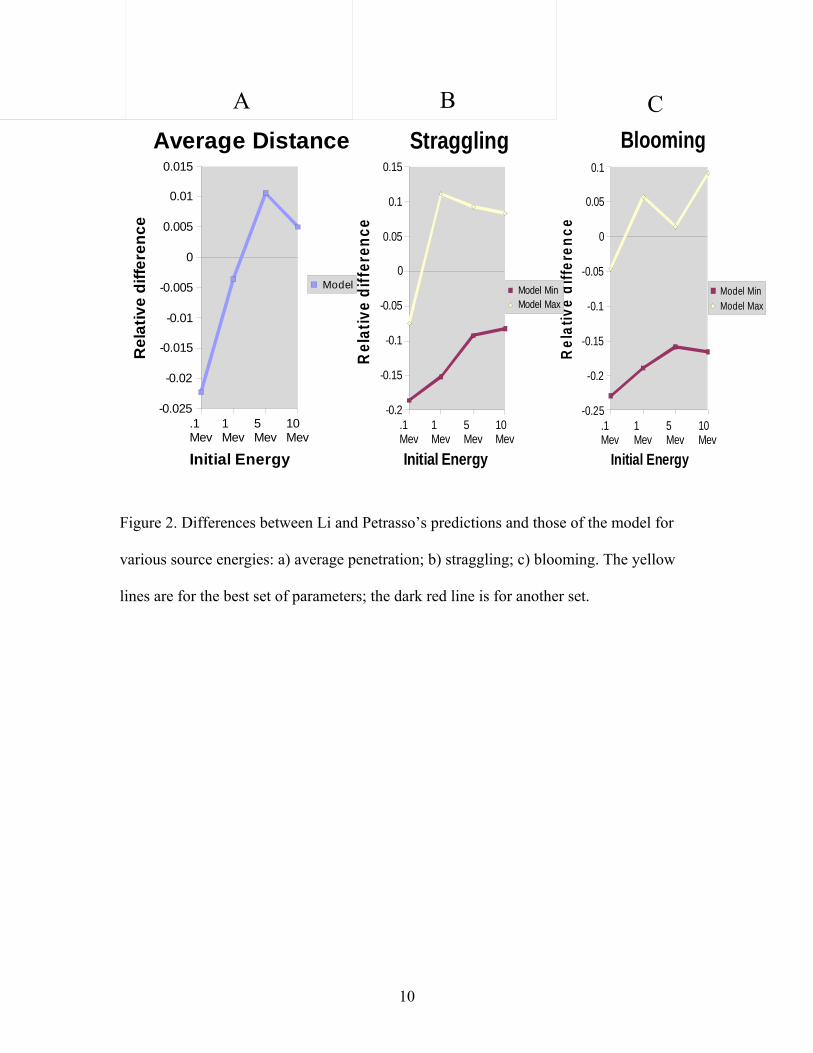
.1 Mev
1 Mev
5 Mev
10 Mev
-0.025
-0.02
-0.015
-0.01
-0.005
0
0.005
0.01
0.015
Average Distance
Model
Initial Energy
Rel
ativ
e di
ffere
nce
.1 Mev
1 Mev
5 Mev
10 Mev
-0.25
-0.2
-0.15
-0.1
-0.05
0
0.05
0.1
Blooming
Model MinModel Max
Initial Energy
Rel
ativ
e di
ffere
nce
C
.1 Mev
1 Mev
5 Mev
10 Mev
-0.2
-0.15
-0.1
-0.05
0
0.05
0.1
0.15
Straggling
Model MinModel Max
Initial Energy
Rel
ativ
e di
ffer
ence
BA
Figure 2. Differences between Li and Petrasso’s predictions and those of the model for
various source energies: a) average penetration; b) straggling; c) blooming. The yellow
lines are for the best set of parameters; the dark red line is for another set.
10
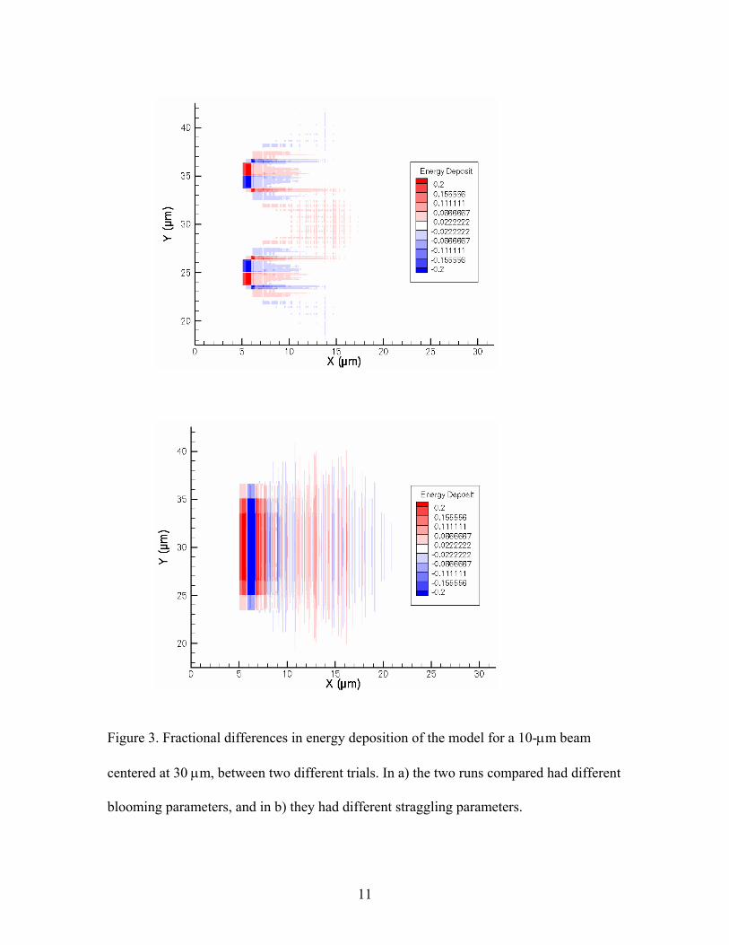
Figure 3. Fractional differences in energy deposition of the model for a 10-μm beam
centered at 30 μm, between two different trials. In a) the two runs compared had different
blooming parameters, and in b) they had different straggling parameters.
11

Fiber Optic Splice Optimization
Elizabeth Gregg

Fiber Optic Splice Optimization
Elizabeth Gregg
Naples Central
LLE Advisors: Shawn Mott, Jon Zuegel
Abstract
Optical fibers transmit data when light waves are propagated through them.
Optical fibers have many applications at LLE, such as the fiber-optic switch module in
the ROSS streak camera.1 It is often necessary to splice two fibers together by a process
called fiber-optic fusion splicing. There are two significant sources of optical power loss
in a fiber: unoptimized splices and losses contributed by the connectorization of the fiber
ends. In order to ensure that a splice is optimized it is necessary to have an apparatus that
will measure just the loss of optical power caused by the splice, account for power
fluctuations of the laser used to test the fiber, and do so accurately enough to measure
low loss. A ratiometer was constructed that measures only the power loss induced from
the splice and can measure losses as low as 0.5%. The ratiometer splits the beam into
two paths. One path serves as the reference (reference fiber), and the other path contains
the fiber being tested (fiber under test). Each fiber has a connector on both ends. Samples
of power measurements are made before and after a fusion splice. This sampling process
allows the energy loss contribution of the connectors to be eliminated. Using the
ratiometer, an amended fusion-splicing program has been shown to reduce the loss in a
splice from between 1.0 dB (20%) and 2.6 dB (45%) to 0.1 dB (~2%).
1
I. Introduction
Fiber splicing is a process by which the cut ends of two optical fibers can be
attached together, resulting in one physical piece of fiber optic cable. Fusion splicing2
involves aligning the fiber cores, heating the two ends, and pushing them together. There
are some alternatives to fusion splicing. Mechanical splicing can be used; however, there
is an alignment loss involved with the mechanical splice process. Fusion splicing, when
optimized, is the best way of connecting two fibers because it minimizes optical power
loss. The theoretical limit for an optimized fusion splice is a power loss of less than 0.01
dB (0.23%).
Some of the most common factors that contribute to a high-loss fusion splice are
low arc power, excessive arc power, incorrect arc duration, uneven heating, and incorrect
hot-push delay. Low arc power or incorrect arc duration will cause insufficient heating
of the fiber. This causes a visible seam in the final splice. This seam acts as a reflective
and refractive surface which in turn creates a high-loss splice. Excessive arc power will
cause deformation in the core of the fibers. Deformation of the core changes the
refractive index at the splice, which can also cause a high-loss splice. Uneven heating
occurs when one fiber is heated and the other is not. This will cause the fiber to fail
during the tension test, i.e. a brittle splice joint. Incorrect hot-push delay settings can
cause the fibers to continue being heated when they are pushed together. This will cause
the fiber to deform at the splice joint. The diameter of the fiber at the splice often
changes under this condition, again leading to a high-loss splice.
The current fusion-splice program used at LLE for multimode fibers was designed
for single-mode fibers of smaller core diameters. When applied to multimode fibers,
where the core diameter is larger, the splice process caused a visible and often warped
2

seam. The appearance of this seam indicated low arc power, incorrect hot push settings,
or possibly both. In order to optimize the fusion splicing process, the program must be
modified, and a ratiometer is needed to test the results. This project involved the
construction of a ratiometer to measure the optical power loss from fusion splices and its
preliminary use to test an improved fusion-splice program.
II. Procedure
A Fitel 3 S183PM fusion splicer was used for the fiber-optic fusion splicing. The
splice process starts with precision alignment of the cores of the fibers. The S183PM
does this by passing light orthogonally through the fiber core and recording the output
with a CCD camera installed on the fusion splice machine. Light that passes through the
center of the core will be un-refracted and the resultant output light intensity will have a
Gaussian type distribution with the peak of the distribution curve corresponding to the
center of the fiber core. The core location is then calculated and aligned appropriately.
The aligned fiber ends are then heated by an electrode arc shot across the ends of the
fibers. The hot push brings the fibers together while the fiber ends are in the molten
state. Improperly heated fibers will not bond well during the hot push. An optimized
splice will have no visible seam through the core; i.e., the splice joint will look
homogeneous.
The ratiometer illustrated in the block diagram of Fig. 1 was developed in order
to test the loss from the splice and not from the connectors or any other source of
potential error. The apparatus starts with a green laser (532 nm) as the light source,
followed by a lens used as a fiber launcher to fill the fiber with higher order modes.
Filling the fiber with higher order modes replicates how the fiber would be used in a
3

typical application at LLE. The splitter is used to split the beam into two paths. Both
sides are followed by a photodiode, so that the light is turned into measurable voltage.
The ratiometer measures the ratio between a reference fiber, which is not moved or
spliced for the duration of the experiment, and the fiber being tested. The other side of
the ratiometer holds the test fiber. The light transmitted across the fiber is sampled
twenty times. The fiber is then cut and spliced and sampled again another twenty times.
By using sample statistics, the mean loss due to connector misalignment can be
calculated. Subtracting this loss from the overall power loss of the spliced fiber will yield
the loss component due to the splice.
Laser
Lens
Splitter
Connector
Test Fiber
Photodiode
Bias Box
Connector
Ref. Fiber
Photodiode
Bias Box
Meter
Fig. 1. Block diagram of the ratiometer used to test fiber splices.
III. Results Results from twenty samples of an un-spliced fiber using FC connectors are
shown in Fig. 2. An oscilloscope and meter were both used for simultaneous data
collection. Statistics of the 20 samples from the scope and meter should yield similar
results, i.e. they should track each other. This eliminates the possibility of one measuring
4

device being “bad”. Data from the reference fiber was also collected and used for the
final data comparison. The reference data were recorded every time that sample data
were taken. Statistics were also applied to the reference samples in order to calculate
mean laser power. The distribution of the reference samples was very narrow and 20
samples resulted in a mean calculation that was equal to the true laser power to a high
accuracy. The very small variations in the signal obtained using the meter and scope
show that the transmission through the fiber can be measured to an accuracy of better
than 0.5%. This allows the loss due to the splice to be measured to an accuracy of 0.5%.
FC Fiber 6
-235.00
-230.00
-225.00
-220.00
-215.00
-210.00
-205.001 2 3 4 5 6 7 8 9 10 11 12 13 14 15 16 17 18 19 20
Sample
mV Scope
Meter
Fig. 2. Signal representing the light transmitted through an optical fiber measured on 20 consecutive samples. The fiber was disconnected and reconnected between samples. The fiber used FC connectors. The consistency of the meter reading allows the fiber transmission to be measured with a 0.5% accuracy.
5
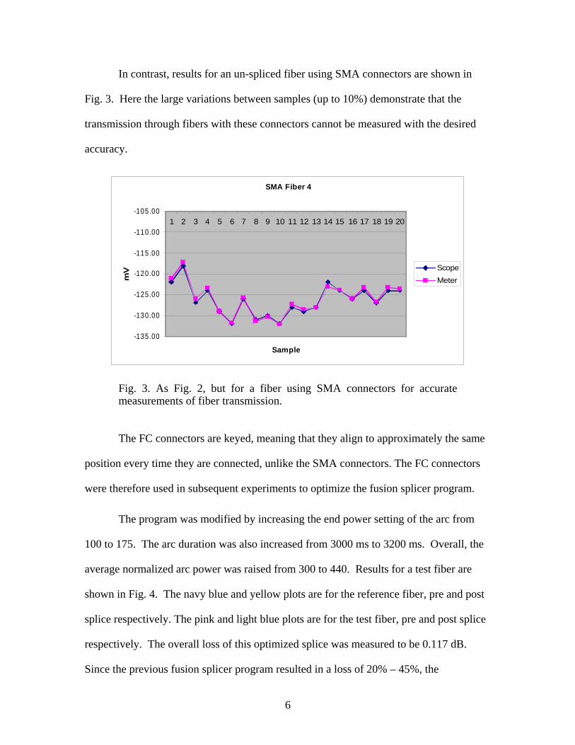
In contrast, results for an un-spliced fiber using SMA connectors are shown in
Fig. 3. Here the large variations between samples (up to 10%) demonstrate that the
transmission through fibers with these connectors cannot be measured with the desired
accuracy.
SMA Fiber 4
-135.00
-130.00
-125.00
-120.00
-115.00
-110.00
-105.001 2 3 4 5 6 7 8 9 10 11 12 13 14 15 16 17 18 19 20
Sample
mV Scope
Meter
Fig. 3. As Fig. 2, but for a fiber using SMA connectors for accurate measurements of fiber transmission.
The FC connectors are keyed, meaning that they align to approximately the same
position every time they are connected, unlike the SMA connectors. The FC connectors
were therefore used in subsequent experiments to optimize the fusion splicer program.
The program was modified by increasing the end power setting of the arc from
100 to 175. The arc duration was also increased from 3000 ms to 3200 ms. Overall, the
average normalized arc power was raised from 300 to 440. Results for a test fiber are
shown in Fig. 4. The navy blue and yellow plots are for the reference fiber, pre and post
splice respectively. The pink and light blue plots are for the test fiber, pre and post splice
respectively. The overall loss of this optimized splice was measured to be 0.117 dB.
Since the previous fusion splicer program resulted in a loss of 20% – 45%, the
6
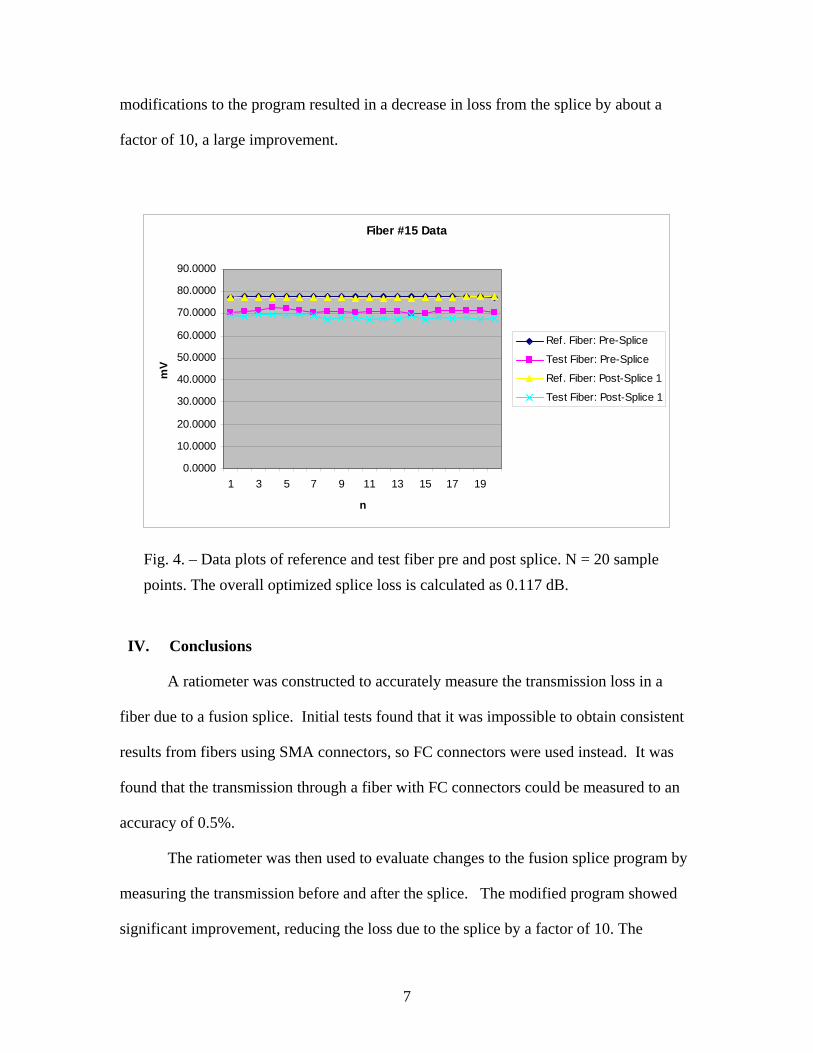
modifications to the program resulted in a decrease in loss from the splice by about a
factor of 10, a large improvement.
Fiber #15 Data
0.0000
10.0000
20.0000
30.0000
40.0000
50.0000
60.0000
70.0000
80.0000
90.0000
1 3 5 7 9 11 13 15 17 19
n
mV
Ref. Fiber: Pre-Splice
Test Fiber: Pre-Splice
Ref. Fiber: Post-Splice 1
Test Fiber: Post-Splice 1
Fig. 4. – Data plots of reference and test fiber pre and post splice. N = 20 sample points. The overall optimized splice loss is calculated as 0.117 dB.
IV. Conclusions
A ratiometer was constructed to accurately measure the transmission loss in a
fiber due to a fusion splice. Initial tests found that it was impossible to obtain consistent
results from fibers using SMA connectors, so FC connectors were used instead. It was
found that the transmission through a fiber with FC connectors could be measured to an
accuracy of 0.5%.
The ratiometer was then used to evaluate changes to the fusion splice program by
measuring the transmission before and after the splice. The modified program showed
significant improvement, reducing the loss due to the splice by a factor of 10. The
7

process is still not fully optimized and more improvements need to be made for the
splices to have the minimum loss possible.
IV. References 1. P.A. Jaanimagi, R.Boni, D. Butler, S. Ghosh, W.R. Donaldson, and R.L. Keck, “The Streak Camera Development Program at LLE,” in 26th International Congress on High-Speed Photography and Photonics, edited by D.L. Paisley, S. Kleinfelder, D.R. Snyder, and B.J. Thompson (SPIE, Bellingham, WA, 2005), Vol. 5580, p. 408. 2. A.D. Yablon, “Optical Fiber Fusion Splicing”, Springer 2005 3. Fitel Inc., 200 Westpark Drive, Suite 190 Peachtree City, GA, 30269 USA
8

Implementing a Knowledge Database for Scientific Control Systems
Daniel Gresh

Implementing a Knowledge Database for Scientific Control Systems
Daniel Gresh Wheatland-Chili High School LLE Advisor: Richard Kidder
Summer 2006 Abstract
A knowledge database for scientific control systems is a powerful tool that allows users to obtain comprehensive information from a single source. A Semantic Web implementation of a knowledge database is intelligent enough to recognize what the user wants to know and present the correct information back to the user. A solid foundation for such a Semantic Web database has been built using the Java programming language, as well as the XML, RDF, OWL, and SPARQL languages. Using this database, a user may already obtain specific, detailed information regarding any aspect of the OMEGA EP Control Systems in an efficient manner from a single source, as opposed to searching through numerous technical and design documents. This foundation of the Semantic Web implementation covers Oracle/SQL, as well as the XML/RDF/OWL/SPARQL aspect. The potential for such a database implementation is substantial. Upon completion, the database will automatically gather information concerning scientific control systems, organize it in an intelligent manner, and present intelligent results back to a user when he or she asks the database a question. Further research into the concept of this Semantic Web implementation will lead to automation of data-gathering; a basic form of artificial intelligence; a single repository for important subject data; and the ability for users to input their own information to expand the database. Introduction The Semantic Web The Semantic Web is a vision for the future of the Web and for the future of information exchange. Rather than simply having information presented to humans, information will be processed in a way that makes it easier and more efficient to find. In the Semantic Web, metadata, or “data about data”, is very useful, as it allows machines to process information rather than present information. By processing information, a machine
1

is able to gather enough useful information to solve problems, which greatly assists any users of such a system.
Due to this ideal, a Semantic Web implementation of a knowledge database will allow a user to find exactly what he or she is looking for with minimal effort and high efficiency, as the information in the database will be processed so the database can present the user with the correct information. Background
LLE has gathered an enormous amount of data and documentation since the start of operations. This data is currently spread over a number of different repositories. Currently there are several hundred active control subsystems, all of which gather and record subject data, which is documented in many ways and stored in one of the data repositories.
The current data repositories include the Product Data Management (PDM) system, word documents, spreadsheets, databases, images, schematics, and events in onboard control memory.
The current PDM system consists of a few general subtopics for the included documents, and then displays links to all the documents, which a user can click on to view a certain document. The PDM system also includes a simple Google search box in which a user can search for certain keywords, and a Google search will be performed on the numerous documents, returning the most relevant documents to the user.
The Oracle database is simply a store for all the data and image information related to OMEGA and OMEGA EP shot operations.
Spreadsheets and other documents are often isolated on personal office workstations. Purpose of the research project
Easily retrieving data from one or any current LLE documentation requires expert knowledge of LLE infrastructure and of the subsystem. For a user to retrieve data using the current system, he or she must follow a number of steps.
For example: the user must determine which data source to browse for the information. The user must already know if the data he or she is looking for is located in the PDM system, or if the data is located in the Oracle database. If a user does not know which one of these sources the data is located in, he or she will have to browse through both databases, which is very tedious.
Second, the user must know where to find the data in a certain data source. If using the Oracle database, the user will
2

need to know which table he or she wants to pull information from. If using the PDM system, the user will need to know which document the information is located in. Otherwise, more tedious searching is required.
Third, the user must parse through the document or table he or she selected, and retrieve the correct data. While this is not a big problem with the Oracle database, it can be very problematic when using the PDM system. Not only does the user need to wade through numerous technical and design documents, he or she must parse the documents manually and extract the correct information. This may lead to even more tedious searching, as a document may not have the specific information a user is looking for, and he or she will have to parse through another document.
Purpose of a knowledge database
A Semantic Web implementation of a knowledge database helps solve this problem by organizing data into a hierarchical structure in which data is organized conceptually and is related to other data through conceptual means. This is also known as an ontology.
After organizing the data in this fashion, the data is stored in a single repository, from where it can be extracted easily. Important data from all sources -- e-logs, technical journals, requirements documents, etc. -- is stored in one location in an organized manner, rather than having the data spread over multiple data sources in which the data is loosely organized.
Furthermore, the data is easily extractable. Rather than manually parsing through numerous documents or tables in a database, a user is able to easily navigate to whatever concept he or she is interested in and view all the related data pertaining to that concept. Also, the Semantic Web implementation enables the user to search the knowledge database using freeform text, or natural language.
Figure1: The World Wide Web Consortium Semantic Web Framework (http://www.w3.org/2001/sw/)
3

As seen in Figure 1, the Semantic Web has many different
building blocks. The basis of the Semantic Web is formed with URI/IRI, or resources. The resources are then structured in a certain way using XML and XML namespaces so the resources can be processed by machines. Then, XML Query and XML schema allow the data to be further refined and queried by providing a slightly more rigid structure; this rigid structure assists XML Query to find information. Finally, using RDF and OWL, which refine the data into an ontological structure, logic and proof are established, which allows machines to draw inferences from the resources, leading to a trusted, stable Semantic Web.
The knowledge database also lets users input their own information. The knowledge database receives manual input, and recognizes when an update to a document or e-log has been made, and reacts accordingly. For example, if a technician makes an entry into an e-log, or an engineer creates a new design document, the knowledge database recognizes this event, obtains the important information from the entry or document, and stores it in the database accordingly.
A Semantic Web implementation is a universal system for processing information. One of the many advantages a knowledge database of this structure has is the ability to connect to other knowledge databases and incorporate that knowledge into useful information. A database of this structure is able to not only contain important subject information from local sources, such as LLE control systems, but also gather and use data and information from external, related sources, further improving efficiency.
A knowledge database of this fashion has unlimited potential for expansion and upgrades. It is a universal repository for important information; this information can be easily extracted due to the data being stored in a machine-readable format.
Furthermore, the tools required to build a knowledge database of this fashion are very easy to acquire and easy to use. Also, the majority of the tools used for this work are open-source tools (free for anyone to use and develop). One of the tools used for this work was not open-source; however it is possible to create a knowledge database with an open-source tool that provides the same features.
The goal of this project was to build a strong, working foundation for a Semantic Web implementation of a knowledge database. This goal was accomplished; an RDF/OWL database was created using Java and the Jena development package for Java, and it is queried using SPARQL through Java and Jena.
4

Research and Analysis
Researching the implementation of a knowledge database that would store the data in a single repository required choosing a small subset of controls. A few diagnostic and control subsystems were chosen for the test case. Much of the implementation used the Calorimeter system. Preliminary research and analysis One of the goals of this project was to analyze methods for creating a knowledge database, and decide which method would work best for the project. Then, the appropriate techniques and tools would be used to create a strong foundation for the knowledge database. Furthermore, the research and analysis was to be done independently. Any tools and/or methods could be chosen that would create a knowledge database in the most efficient manner. Initially, fourteen different languages were investigated. Eleven of them are listed in Table 1, together with their purpose, and the reason why they were or were not selected for use.
Many different tools and software packages were analyzed that might be useful, including Altova SemanticWorks, Protégé OWL, Jena, Lixto, Inxight, Evermap, Adobe Online Tools, KAON, JTP, Twinkle, Metadata Miner, Pellet, Omnipage, PDF Extraction, PDF to all, PDF Extractor API, pOWL, OWL API, PDF Metadata, VorteXML, and XML Army Knife. Tools were looked at for writing RDF/OWL, for performing SPARQL queries, for writing PHP, and for extracting data from documents. Developing a data mining tool was a large concern. In order for quality, reliable data to be extracted from the numerous documents and sources that exist at LLE, some type of extraction tool would have to be developed. To determine how to create such a tool, the field of data mining and extraction was investigated. Studies of data mining and extraction methods led to one conclusion: the tool would have to be custom developed specifically for LLE; a pre-existing data mining tool would not work. This tool will be the subject of future work. The World Wide Web Consortium (W3C) Web site proved to be a very valuable source of information,1 in particular on the languages of RDF, OWL, XML, and SPARQL. Work related to this project is found in Refs. 9-12.
5
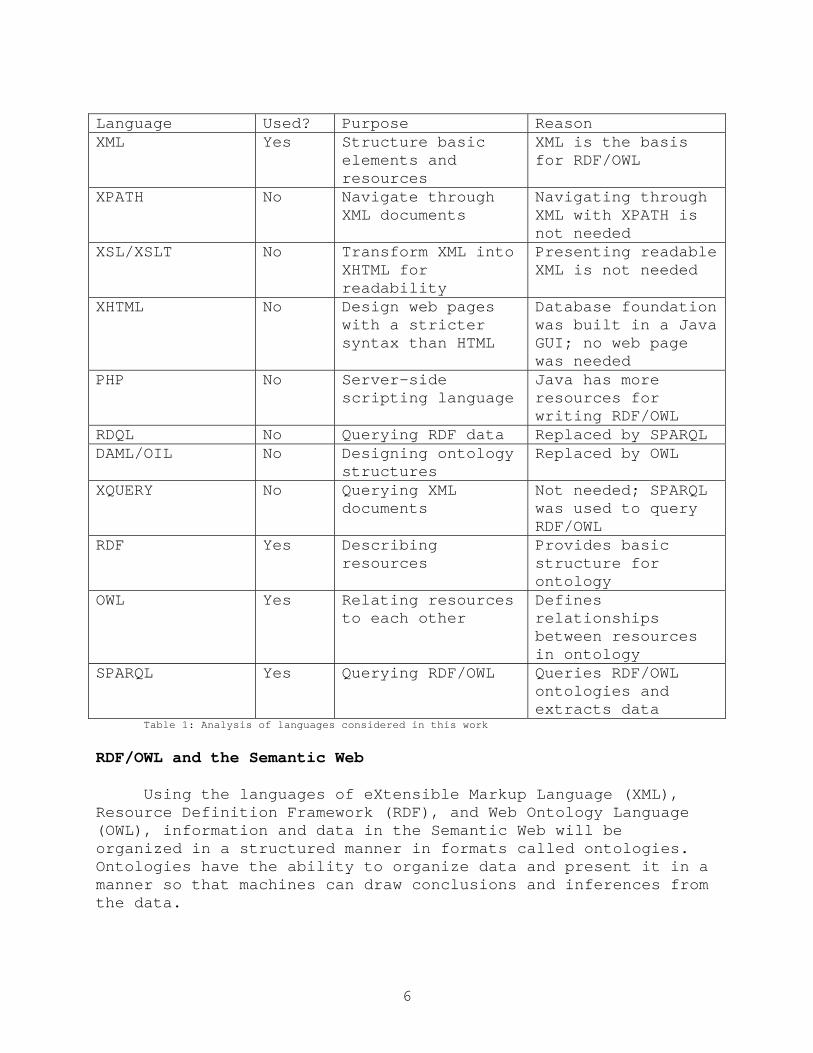
Language Used? Purpose Reason XML Yes Structure basic
elements and resources
XML is the basis for RDF/OWL
XPATH No Navigate through XML documents
Navigating through XML with XPATH is not needed
XSL/XSLT No Transform XML into XHTML for readability
Presenting readable XML is not needed
XHTML No Design web pages with a stricter syntax than HTML
Database foundation was built in a Java GUI; no web page was needed
PHP No Server-side scripting language
Java has more resources for writing RDF/OWL
RDQL No Querying RDF data Replaced by SPARQL DAML/OIL No Designing ontology
structures Replaced by OWL
XQUERY No Querying XML documents
Not needed; SPARQL was used to query RDF/OWL
RDF Yes Describing resources
Provides basic structure for ontology
OWL Yes Relating resources to each other
Defines relationships between resources in ontology
SPARQL Yes Querying RDF/OWL Queries RDF/OWL ontologies and extracts data
Table 1: Analysis of languages considered in this work
RDF/OWL and the Semantic Web Using the languages of eXtensible Markup Language (XML), Resource Definition Framework (RDF), and Web Ontology Language (OWL), information and data in the Semantic Web will be organized in a structured manner in formats called ontologies. Ontologies have the ability to organize data and present it in a manner so that machines can draw conclusions and inferences from the data.
6

The Semantic Web is not pure artificial intelligence. Rather, as previously stated, it will use data that can be processed by machines to solve questions and perform tasks. The three “main” languages that the Semantic Web concepts are based upon are XML, RDF, and OWL. These languages work together to describe resources and relate them to each other so that machines can process the information. These languages do not exist to provide information to humans, but rather to provide information to machines, so the machines can then determine what information is useful to provide to humans. By structuring the resources using RDF/OWL and creating an ontology, numerous resources can be related to each other so they can easily be processed by a machine. An example of such a use is shown in Figure 2, which represents a small subset of OMEGA EP control systems. “IR Cal System” forms the base for the subtopics under it. These subtopics branch off into many different subtopics. However, due to the reasoning capabilities of RDF/OWL ontologies, although a subtopic such as “TSF Cal 1” may be a direct subtopic of “TSF Cals”, a machine can reason that “TSF Cal 1” is also a subtopic of “IR Cal System”.
Figure 2: Structure of resources.3 Cal: Calorimeter; GCC: Grating Compression Chamber; UC: Upper Compressor; LC: Lower Compressor; TSF: Transport Spatial Filter; SPPOL: Short-Pulse Polarizer; POL: Polarizer
RDF is structured as a series of graphs called “triple graphs”. These triple graphs, or triples, are what make it possible for machines to process RDF. A triple is a basic description that is read in the form: subject, predicate, object. For example, one could use RDF to specify the title and author of a certain book, by creating a triple with subject Example Book; predicate author; and object John Smith. This would then be read: the author of Example Book is John Smith.
7

Triples are instrumental in creating a database structure for LLE data. By using the triple format, data is stored in RDF where it can easily be extracted with SPARQL. For example, by creating a triple with subject “SPPOL Calorimeter Location”; predicate “information”; and object “The SPPOL Calorimeter is located between beamlines 1 and 2”, one could read: the information of SPPOL Calorimeter Location is, “The SPPOL Calorimeter is located between beamlines 1 and 2”. Planning and Design Preliminary design Java was chosen as the language to program the database. The database had to be flexible, easily modifiable, and transportable across the Web to a variety of operating systems for easy access.
Java is an object-oriented programming language. In other words, an application is a series of individuals, or objects, rather than simple commands to the computer.3 Using Java it is relatively simple to keep a database structure organized and functional. Java provides a simple, object-oriented structure, whereas PHP does not. PHP is a server-side scripting language. There are tools available that allow RDF/OWL ontologies to be built using PHP, but Java’s object-oriented nature allows the RDF/OWL to be built in a more efficient, modifiable manner. Furthermore, there are more resources available to assist in building RDF/OWL ontologies with Java than there are with PHP. RAP, the most common PHP development kit for writing RDF/OWL, has far less support and usage than Jena, the most common Java development kit for writing RDF/OWL. Because of this, using Java allows the programmer to learn the structure and functions faster, resulting in greater efficiency. Tools To develop an RDF/OWL database in Java, the Jena development package was used9. This is an external library for Java that allows for the programming and development of RDF/OWL databases. Jena also has support for the SPARQL querying language in its Application Programming Interface (API), which greatly assists when performing SPARQL queries against the RDF/OWL database. Furthermore, some free tools were downloaded that would allow for the easier development of a Java application to create an RDF/OWL ontology. These include the Eclipse and Netbeans
8
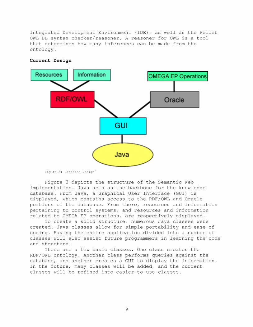
Integrated Development Environment (IDE), as well as the Pellet OWL DL syntax checker/reasoner. A reasoner for OWL is a tool that determines how many inferences can be made from the ontology. Current Design
Figure 3: Database Design3
Figure 3 depicts the structure of the Semantic Web implementation. Java acts as the backbone for the knowledge database. From Java, a Graphical User Interface (GUI) is displayed, which contains access to the RDF/OWL and Oracle portions of the database. From there, resources and information pertaining to control systems, and resources and information related to OMEGA EP operations, are respectively displayed. To create a solid structure, numerous Java classes were created. Java classes allow for simple portability and ease of coding. Having the entire application divided into a number of classes will also assist future programmers in learning the code and structure.
There are a few basic classes. One class creates the RDF/OWL ontology. Another class performs queries against the database, and another creates a GUI to display the information. In the future, many classes will be added, and the current classes will be refined into easier-to-use classes.
9

Current Status
Currently, a strong foundation for the database has been created, and a working, functional prototype of the database was successfully demonstrated. The database is currently a simple Java Archive (JAR) file for ease of use, and will be uploaded to the local intranet.
Figure 4 shows the structure of the graphical user interface for the Semantic Web Knowledge Database. A simple tree diagram is contained on the left side that allows a user to select the topic he or she desires. When the user clicks on a certain topic in the tree diagram, the information associated with that topic is displayed, as shown in Figure 4.
Figure 4: The Semantic Web knowledge database GUI
The Java code for the database has been created in such a
way that it will be very easy to modify and expand upon. The code for the database has unlimited potential to evolve and expand, allowing multitudes of new features (see next section).
10

An ontology in OWL Full, for maximum ease of use, has been created that stores data about a small section of control systems: calorimetry. A GUI has been created that allows for easy searching of that database. Functionality has been added to the database that allows it to search the Oracle database about OMEGA EP operations.
The user currently browses through the information in the ontology by using a tree diagram. When the user selects a certain node on the tree, a SPARQL query is executed against the RDF/OWL ontology, which returns the necessary information and presents it to the user. The tree diagram allows the user to easily specify the information he or she is looking for, and view it in a simple, efficient manner. Future Features As the project moves forward, additional features will be designed and implemented. Further research into the field of artificial intelligence and the Semantic Web will lead to more advanced features that can be implemented at LLE. Much of this research may take place at MIT’s Computer Science and Artificial Intelligence Laboratory, where extensive research is already being done. In the coming year, a user will be able to enter freeform text questions into the database and receive the correct answer, rather than using a tree diagram. The database will gather all information automatically and will eliminate redundant information. Also, it will organize the gathered information in an ontology, where it can be structured in an intelligent manner. There will also be the ability for users to enter their own information into the database, expanding it with important information. The database will be able to recognize what information is important or not, and take action accordingly. The database will be a single repository for important information. Rather than having numerous sources for data, all data will be stored in one central location where it can be easily and efficiently extracted. The database will have the ability to be expanded and upgraded to fit any reasonable need, and ultimately improve our knowledge of control systems and other important areas. Acknowledgements
I’m excited to continue this fascinating project during my senior year at Wheatland-Chili High School. I thank LLE – in particular, Richard Kidder, Robert McCrory, and Stephen Craxton – for giving me this wonderful opportunity. I would also like to
11

thank Ivan Herman, the director of W3C’s Semantic Web Activity, and Jim Hendler, a professor at the University of Maryland, who is a chair on W3C’s Semantic Web Activity, for their assistance during the course of the summer.
References 1. http://www.w3.org/ 2. http://en.wikipedia.org/wiki/Object-oriented_programming 3. PowerPoint presentation on the summer research project:
http://www.seas.rochester.edu/~gresh/dangresh/DGreshRev3.ppt 4. http://www.w3.org/2001/sw/ 5. NASA ScienceDesk white paper:
http://ti.arc.nasa.gov/publications/pdf/ISWC-04%20SemanticOrganizer%20Paper%20pub.pdf
6. Additional notes and design ideas from notes taken over the summer: http://www.seas.rochester.edu/~gresh/dangresh/LLE _Semantic_Web.pdf
7. MIT’s CSAIL Decentralized Information Group Semantic Web Projects: http://dig.csail.mit.edu/
8. Jena: http://jena.sourceforge.net/ 9. Personal Publication Reader: http://www.personal-
reader.de/semwebchallenge/sw-challenge.html 10. NASA ScienceDesk: http://sciencedesk.arc.nasa.gov/ 11. Platypus Wiki: http://platypuswiki.sourceforge.net/ 12. Swoogle: http://challenge.semanticweb.org/
12

Realtime Focal Spot Characterization
Matt Heavner
Realtime Focal Spot Characterization
M. Heavner Advised by Dr. Christian Stoeckl
Laboratory for Laser Energetics
University of Rochester 250 East River Road Rochester, NY 14623
March 13, 2007
Abstract
Short-pulse laser-plasma interaction experiments are carried out at the University of Rochester's
Laboratory for Laser Energetics (LLE). In these experiments a short (< 1 ps) laser pulse is focused to a
small (<4 µm) spot on a solid target, rapidly creating a plasma. During alignment, the focal spot has to
be located and characterized. A CCD camera provides high-resolution image data of the focal spot in
analog format that is converted into a digital signal with a framegrabber, allowing it to be used by
software. A program has been developed using the C and Java programming languages that accesses
the framegrabber, acquires images, and interprets acquired data. It is able to locate the focal spot from
the CCD data, graph the data, zoom into and autoscale the image, and infer the size of the focal spot.

1 Introduction
Figure 1.1: LLE's MTW Experimental Setup
In the University of Rochester's Laboratory for Laser Energetics (LLE), short pulse laser-
plasma interaction experiments are carried out. In LLE's experimental setup (shown in Figure 1.1), a
laser beam is sent into a chamber, reflected off a flat mirror and an off-axis parabolic mirror, and
focused by a focusing mechanism on a small target. In the alignment of this setup, a requirement to
locate and characterize laser focus points arises. Charge-coupled device (CCD) cameras, connected
to microscopes, are used to provide real time, high-resolution image data of these points.
CCD cameras are used extensively within LLE experimental setups. CCDs provide high-
resolution images and are up to 70% more photosensitive to incident light than photographic film. A
CCD is composed of an array of photosensitive capacitors. During exposure, charge is transferred to
non-photosensitive cells that are located in between active rows. The charge in these storage cells is
shifted along the row one row at a time to form a video signal. This occurs while the active cells are
being exposed to produce the next frame.
To access and interpret image data, a framegrabber must be installed in the client computer that
is accessing the CCD camera. A framegrabber converts the analog video signal from the CCD to a
digital signal, as shown in Figure 1.2, that is usable by a computer. The framegrabber used in the
development of this program was a DT3155, created by Data Translation, Inc.1 The DT3155
2

provides four multiplexed monochrome inputs, 8-bit digitization, programmable black and white
levels, real-time image thresholding and image scaling and clipping.1
Figure 1.2: A CCD camera, DT3155 framegrabber and DTConrol in use2,3,4
A program has been developed to actively locate and characterize a laser focal point using data
acquired from a framegrabber that is attached to a CCD camera. It uses both the Java and C
programming languages and the open-source Linux DT3155 driver5, modified to fit LLE needs. This
program (DTControl) has been designed to be as self-intuitive as possible, allowing a scientist to
start using it without previous knowledge of its inner workings and to still acquire necessary and
useful information. Tools and features have also been added to allow the program to adapt to
different experimental environments. The program has been designed to accommodate future
upgrades.
2 Programming Technologies
Many operating systems are in use within LLE. Because of this, program code must be
portable so that it may be used on different platforms. This program was designed and tested on a
Linux machine. The GNU/Linux operating system6 has proven to be very successful and stable, and
is used frequently within LLE because it allows code to be portable. The Java and C programming
languages, along with the Java Native Interface, were utilized in the creation of this program. Java,
which began as a Sun Microsystems project termed Oak that sought to provide an alternative to
C/C++ 7, allows for the creation of code that can be used on many platforms. This is possible through
the use of the Java Virtual Machine (JVM), which itself is platform-specific. Java code is created
3

and, when run, is interpreted by the JVM and executed on the desired platform. Methods to access
hardware were intentionally left out of the Java programming language in order to provide
portability across varying hardware. The C programming language, developed in 1972 in the Bell
Telephone Laboratories by Dennis Ritchie for use on the Unix operating system8, is known as a
lower-level programming language that provides direct access to computer memory and other
intricacies. Code developed in C is platform-specific and is often more efficient than code written in
other languages, such as Java, as it doesn't have overhead code, such as Java's JVM. It is useful
when interfacing hardware or operating systems directly.
Figure 2.1: The Java Native Interface allows native languages to communicate with Java
In the event that a Java program must access platform-specific features, or code written in a
lower-level language, the Java Native Interface must be used (see Figure 2.1). The Java Native
Interface provides a way for Java code to utilize software libraries written in a native language, e.g.,
C or C++9. In the case of DTControl, it was used to provide the Java code with access to the
DT3155 framegrabber.
3 Program Requirements
Requirements of the program needed by the user (LLE scientists) include the ability to locate
and track a laser focal point, to measure and characterize such a point via graphing and interpretation
4

of data, to save and load images, and to adjust to various environments. The user must also be given
the option of changing the accuracy of these features. Internally, the program must be robust and
accurate, as many other process and tools are used concurrently on LLE computers.
4 Algorithm Design and Analysis
Algorithms were developed to allow for zooming, the location of a laser focal point, the
measurement of a laser focal point, and auto-scaling of the image intensities to allow for better
contrast.
4.1 Digital Zoom Algorithm
Upon a request from a user to zoom into a certain portion of an image, a boxed area of data
surrounding the clicked point is partitioned. Pixels found within this area are expanded so that the
selected portion of the image fills the entire viewing area. This may only be done a certain
maximum amount of times, as zooming into a portion of the image too far will make it appear
overly pixelated.
4.2 Focus-location Algorithm
Other algorithms and program aspects are dependent upon an accurate focal-spot center being
found. This algorithm must be efficient because it is run very frequently (defaulted at every five
frames). The process of finding the center involves two stages. First, an approximate center is
located. This result is used in the second step that narrows the given information into an accurate
result.
The first stage, location of the approximate center, works as follows: First, every nth line (an
undersampling rate of n) is checked for pixels of intensities greater than a certain value. These
values are stored in an ArrayList, a dynamic storage structure. Second, the surrounding intensity
(defined as the average over a six by six pixel area) of each previously found pixel is calculated. The
5

pixel with the greatest surrounding intensity is the approximate center.
Figure 4.1: Second stage of the focus location algorithm
The location of this approximate center is then sent to the second stage of the process, which
uses the formula shown in Figure 4.1 to obtain the spot center (x,y) as the centroid (weighted
average) over a region of nx by ny pixels. Here, x represents the X coordinate, y the Y coordinate, z
the pixel intensity, and nx and ny the number of rows and columns checked, respectively. This
method has been found to be highly accurate.
Figure 4.2: Accuracy and runtime for spots with a varying undersampling rate
Figure 4.3: Accuracy and runtime for large spots with a varying undersampling rate
The main factor determining the efficiency and runtime of this algorithm is the undersampling
rate n. The program allows the user to set the rate up to 10, which means that every 10th line is
6

checked. The algorithm was run one thousand times at each undersampling rate, with noise levels
and spot-center locations randomized. Figure 6.2 shows two generated images used in this testing
process. The percent accuracy, or average error over the thousand runs when attempting to locate the
center, and the associated runtime are shown in Figures 4.2 and 4.3 as functions of the
undersampling rate. A balance between efficiency and accuracy must be determined. Clearly, the
larger the focal spot, the greater one can afford to increase the undersampling rate and still remain
accurate, thereby saving CPU cycles.
4.3 Focal-measurement Algorithm
Figure 4.4(a): Experimental image of a focal spot, indicating the center of the spot and lineouts
through the center of the spot in the horizontal and vertical directions
(b): Autoscaled image, with the center intensity scaled to 256.
An experimental focal spot is shown in Figure 4.4(a), needing to be measured and autoscaled
so that it might have a contrast that is easier to view.
7

Figure 4.5: Full width at half maximum for a given curve10
When characterizing a focal point, knowledge of the full width at half maximum (FWHM) is
often very useful. This value, indicated graphically in Figure 4.5, is the distance between two points
on a curve whose value is half that of the maximum value of the curve.11 The algorithm goes
through the following process: First, the intensity at the located focal center is obtained and the half-
maximum value is calculated. Second, the algorithm traverses through the data vertically and
horizontally until the points equal to or less than the half-maximum value are found. Noise is
avoided in this step by checking points beyond the point in question to see if a decrease in intensity
is consistent or rather noise-induced. Third, the distance between these two located points is
calculated. The thin green lines shown in Figure 4.4 indicate the FWHM.
The ability of the program to auto-scale image data is often imperative to providing a viewable
image contrast. An algorithm to auto-scale pixel intensities has been developed. It calculates the
auto-scaled intensity I’ as I*(256/m) where I is the original intensity and m is the intensity at the
focal center. The auto-scaled image of Figure 4.4(a) is shown in Figure 4.4(b).
8

5 Program Design
DTControl follows the object-oriented model of programming, creating various objects that
carry out different tasks. Figure 5.1 shows DTControl’s class layout, subdivided into classes of
similar purpose.
Figure 5.1: Program class hierarchy, subdivided into objects serving various purposes
The device classes provide an interface for accessing a CCD camera. They include DTCamera,
which represents a CCD camera, containing data structures to hold image data and abstractions to
acquire images, and DTDev, which provides access through the Java Native Interface to a C library.
This library interfaces with a Linux driver that provides access to a DT3155 framegrabber.
The display classes are associated with the proper interpretation and display of data acquired
from device classes. They include DTGui and DTView. DTView is responsible for displaying the
information from one DTCamera. DTGui represents the entire user interface of the program, and
assembles and displays a DTView and other components.
The focus location classes are responsible for the implementation of the focus location
algorithm. SpotLocator provides algorithms for locating the laser spot and for calculating the
FWHM values. ImageGenerator generates random images that are used to simulate laser focal spots.
9

The central classes control and synchronize other program features. DTSave and DTLoad save
and load still images and DTSettings provides access to many program settings. Finally, DTControl
controls all other classes and synchronizes GUI and camera updates.
Figure 5.2: The user interface and options, designed to be self-intuitive
A user interface has been developed that allows the user to select many features. Selecting an
appropriate color gradient for images such as Figure 4.4 is important, as protective glasses used in
laboratories often block certain colors. Color gradients, as well as the undersampling rate and
algorithm sensitivity, can be changed by the user. Other features, such as a pixel intensity bar,
displayed graphs, the calculation of FWHM values, the display of axes, and more, can also be
enabled and disabled.
6 Program Testing
Figure 6.1: A two-dimensional Gaussian function12
A process whereby the program could be tested outside the real environment was needed
10

because it wasn’t always possible to test the program in the real environment. The program was
given the capability to generate virtual images to display from a virtual CCD camera. These images
were composed of a two-dimensional Gaussian function (see Figure 6.1) with added noise, which
produces a very natural distribution that appears as an ideal focal spot. The noise was added by
augmenting a random number of pixels, between 0 and 1/5 of the image’s area, by a random value
between 1 and 255. Examples of such images are shown in Figure 6.2, 6.2(a) with tracking enabled
and 6.2(b) with tracking disabled.
(a) (b)
Figure 6.2: Test images produced from two-dimensional Gaussian functions with added noise.
(a) Tracking enabled; (b) tracking disabled.
7 Conclusion
Short-pulse laser plasma interaction experiments are carried out within LLE. They require a
program that can locate and characterize a laser focal spot in real time. Such a program has been
developed using the C and Java programming languages. The design of the program assigns
different roles to various objects, creating a structured design that is easy to upgrade or alter in the
future. The program and its various algorithms have been tested and proven to be accurate in both
simulated and real laboratory environments. The program has already been used in the alignment
and testing of lasers within LLE's Laser Development Laboratory and will continue to be used
11

during experiments at LLE.
8 Acknowledgments
I would like to thank my advisor Dr. Christian Stoeckl for his guidance, hints and words of
advice during the progression of this project. I would also like to thank Dr. R. Stephen Craxton for
providing the opportunity to pursue research at The University of Rochester's Laboratory for Laser
Energetics this past summer.
9 References and Sources
1. DT3155 – Full Specification. Data Translation, Inc. 16 Aug. 2006 <http://www.datx.com/products_hardware/prod_dt3155_spec.htm>.
2. Online Image. CCD Camera. 6 Oct. 2006
<http://www.ni.com/third_party/sony/pdf/xcsT70_ce.pdf#search=%22xcst70_ce%22>. 3. DT3155 – Full Specification. Data Translation, Inc. 16 Aug. 2006
<http://www.datx.com/products_hardware/prod_dt3155_spec.htm>. 4. Online Image. Computer Clip Art. 14 Aug. 2006
<http://www.sbac.edu/~tpl/clipart/Technology%20and%20Machines/computer%2001.jpg>. 5. DT3155 Framegrabber Linux Device Driver. Version 1.8. <http://sourceforge.net/projects/dt3155a>. 6. The Linux Kernel Archives. <http://www.kernel.org>.
7. Kabutz, Dr. Heinz. Java History 101: Once Upon an Oak. 30 Jan., 2003. 24 Aug. 2006
<http://www.devx.com/Java/Article/10686/0/page/1>.
8. Aitken, Peter. Learning C. Carmel: SAMS, 1991.
9. Stearns, Beth. Trail: Java Native Interface. 21 Aug. 2006 <http://www.iut-info.univ-lille1.fr/docs/tutorial/native1.1/index.html>.
10. Online Image. Full-width at half-maximum. 10 Aug. 2006
<http://cfao.ucolick.org/EO/steinb/education_outreach/demoweb/home/FWHM.gif>.
11. Weisstein, Eric W. “Full Width at Half Maximum.” MathWorld-A Wolfram Web Resource. 10 Aug. 2006 <http://mathworld.wolfram.com/FullWidthatHalfMaximum.html>.
12. Online Image. 2d gaussian. 16 Aug. 2006
<http://local.wasp.uwa.edu.au/~pbourke/other/distributions/gaussian6.gif>.
12

Neutron Transport Calculations Using Monte-Carlo Methods
Sean Lourette

Sean Lourette
Neutron Transport Calculations Using Monte-Carlo Methods
Sean Lourette Fairport High School
Advisor: Christian Stoeckl
Laboratory for Laser Energetics University of Rochester
Summer High School Research Program 2006
Abstract
Fusion reactions from direct-drive inertial confinement fusion experiments at the Laboratory for
Laser Energetics (LLE) release large amounts of stored nuclear energy. Most of it is given off as
energetic neutrons. Plastic scintillators are used as detectors for these neutrons. The neutrons that
interact with the scintillator produce photons that are recorded using a photomultiplier tube on a fast
oscilloscope. The detector has a lead shield used to block x-rays that would flood the detector with
energy. The neutrons travel throughout the target area interacting with several structures, such as the
chamber wall, that significantly affect the neutron transport. In order to understand the effects of the
target chamber and lead shield on the detected neutron signal, a Monte-Carlo simulation program
(Geant4) was used to simulate neutron interactions. Geant4, a toolkit designed to calculate particle
interactions with matter, is used predominantly in high-energy, nuclear, and accelerator physics. By
changing the geometric dimensions and material properties of the structures in the target area, effects
that cannot be tested experimentally have been simulated. It was found that the lead shield and the
target chamber have a minimal effect (< 1%) on the full width at half maximum (FWHM) of the
neutron signal.
1

Sean Lourette
1. Introduction
The long-term goal of fusion research is to design a sustainable fusion energy source that can
produce energy cleanly from common fuel sources. The Laboratory for Laser Energetics conducts most
of its experiments and research on the OMEGA laser system, which consists of 60 symmetrically
oriented, high-power laser beams focused onto a target to obtain internal confinement fusion. The
targets are composed of frozen hydrogen isotopes deuterium (2H) and tritium (3H), the most common
reactants for fusion reactions. When the nanosecond laser pulse strikes the target, the outer shell rapidly
expands, compressing and heating the fuel creating temperatures similar to those in the center of sun.
1.1 Neutron Production
Most of the energy from fusion reactions is given off in the form of energetic neutrons. These
neutrons can be created by two distinct types of fusion reactions: deuterium-tritium (DT) and
deuterium-deuterium (DD). DT reactions yield a 14.1 MeV neutron and a 3.0 MeV alpha particle,
while DD reactions yield either a 2.45 MeV neutron and a 0.825 MeV helium-3 nucleus, or a 3.0 MeV
proton and a 1.0 MeV triton.1
In order for the reaction to occur, the relative velocity of the reactants must be large enough to
overcome the Coulomb force and release the stored nuclear energy. This energy is distributed between
the two products as given above; however, since the net momentum of the reactants is not constant, the
actual distribution of the energy between the two products varies in order to conserve momentum and
energy. The resulting neutrons from each type of reaction (DD, DT) have a Gaussian distribution of
energy such that the mean energy is equal to either 2.45 MeV (for DD) or 14.1 MeV (for DT). The
width of the energy distribution is proportional to the square root of the temperature of the reactants.
This temperature is significant because a high plasma temperature is necessary for the fusion reactions
to occur.
2

Sean Lourette
1.2 Neutron Detection
In order to measure the width of the spread of neutron energies, the OMEGA laser system uses
plastic scintillators (Bicron BC-422Q2) to measure the spread in the neutron time of flight, which can
be correlated to a distribution of energies. To prevent the intense bremsstrahlung that would be
produced in the detector from x-rays, a lead shield is placed directly in front of the detector. The cross
section between x-rays and lead is much greater than the cross section between neutrons and lead,
greatly decreasing the intensity of the x-rays entering the scintillator while having a significantly
smaller effect on the neutrons. Neutrons produce a photon signal in the scintillator by transferring
energy to a nucleus (hydrogen or carbon), whose electrons are ionized from the energy. These ions and
electrons excite and de-excite nearby atoms, emitting photons, which are converted to current in a
photocathode. The current is amplified using a microchannel plate and measured with a fast
oscilloscope.3 Figure 1 illustrates this process.
Figure 1: Scintillation process – A neutron collides with the nucleus of an atom such as hydrogen. The atom becomes ionized and excites and de-excites nearby atoms, emitting photons. The photons
generate current in a photocathode. The current is amplified by a microchannel plate and read by a fast oscilloscope.
Although the lead shield reduces x-ray data, it also scatters neutrons, which could significantly
alter the FWHM, used to measure the time of flight spread of the arriving neutrons. Because the
detector requires the lead shield in order to collect data, the effect of the shield on the neutron signal
3

Sean Lourette
cannot easily be determined experimentally. It is also extremely difficult to determine theoretically.
The same holds true for the aluminum target chamber, which is required to create a vacuum to ensure
that the focused laser energy reaches the target with its beam quality preserved. The primary goal of
this study is to model the effects of the target chamber and lead shield on the neutron time of flight
spread.
1.3 Geant
Geant4 is a Monte-Carlo simulation toolkit for the passage of particles through matter. A
Monte-Carlo simulation uses random or pseudo-random numbers and interaction probabilities to
simulate an experiment. Geant tracks the energies of each particle (projectile) until it decreases below a
certain value known as the “cut value.” At this point, Geant no longer tracks that energy and disperses
it among the local particles, increasing the thermal energy of the volume. Any particle near a boundary
is tracked below the cut value because there is a significant probability that the particle will travel into
the next volume. Geant allows the user to select different physics processes, cut values, magnetic
fields, material types, and many other settings in order to simulate the desired experiment. Like an
experiment, Monte-Carlo simulations generate data that requires statistical analysis. The simulations
also require extended runtimes in order to create meaningful data.
4

Sean Lourette
2. The Program
Using the Geant toolkit, a program was written to
simulate the neutron transport in the target area. The LHEP5
physics library was used to manage the physics processes,
including hadronic and electromagnetic processes. The
hadronic processes model strong-force interactions between
neutrons and nuclei, while the electromagnetic processes
model the ionization of electrons. The conversion from
electron energy to photon energy was not modeled because the
conversion efficiency is known to be a constant ratio.
The program constructs geometries and their
corresponding materials, representing the structures in the
target area that contribute the most to neutron scattering. The
dimensions and materials are shown in Figure 2. Figure 3
illustrates the structural setup. The concrete walls have a minimal effect on the neutron detection and
were added for completeness. The neutrons that do scatter off the chamber walls and reach the detector
arrive much later than the significant neutron signal. The scintillator was constructed as a “sensitive
detector” meaning that it records energy deposited within the volume by each particle. The program
records specific information for each quantity of energy deposited that can be statistically analyzed.
Dimensions Room Length = 30 m Room Width = 15 m Room Height = 15 m Chamber Thickness = 8.89 cm Chamber Outer Diameter = 6 m Detector Distance from Target = 12 m Detector Diameter = 4 cm Detector Height = 1 cm Shield Diameter = 4 cm Shield Height = 2 cm Materials
Detector Material = Plastic Chamber Material = Aluminum Wall Material = Concrete Room Material = Air Shield Material = Lead
Figure 2: Default dimensions and materials used for the simulations.
For all simulations, 14.1 MeV mono-energetic neutrons were projected from the center of the
target chamber. Mono-energetic neutrons were used to clearly observe the extent of the neutron
scattering.
5

Sean Lourette
Figure 3: Materials used in the program – Each region was assigned a material with a temperature, density, and pressure.
3. Test Simulations
In order to confirm that the results produced by Geant are accurate, two simple tests were
performed. In each test, all materials except the detector itself were changed to vacuum, and mono-
energetic neutrons were launched directly at the detector. In the first test (Figure 4), which measured
the energy deposition over time, the results were as expected. At the front of the signal, there is a very
steep increase in the deposition energy. The signal then decreases exponentially over time until the
neutrons reach the end of the detector, when the signal drops sharply. The remainder of the graph is
background generated by neutrons that lose some of their energy near the front and deposit additional
energy near the back at a time after the signal drop. The 0.8 ns FWHM correctly corresponds to the
height of the 4 cm detector divided by the speed of a 14.1 MeV neutron (5.14 cm/ns).
6

Sean Lourette
Figure 4: First Test – Energy deposition signal for 14.1 MeV neutrons through a 4 cm detector placed 10 m away from the target. The sharp rise and drop of the signal correctly correspond to the times at which
the non-interacting neutrons pass through the detector. Between these times, the signal drops off exponentially.
A second test was performed to calculate the mean-free path of neutrons through a plastic
scintillator. The detector was lengthened to 200 cm and all other conditions were the same as in the
first test; however, instead of recording the energy deposition, the distance traveled by each neutron
before its first interaction was recorded. The data was used to create a graph (Fig 5) of the percentage
of non-interacting neutrons (y) versus length (x). The graph is well fit by an exponential of the
form: bx
ey −= , where b is the mean-free path. The mean-free-path value produced by Geant is 11.00
cm, while the literature value is 10 cm.6 This favorable comparison confirms that Geant is producing
meaningful data.
7

Sean Lourette
Figure 5: Second Test – The attenuation graph for 14.1 MeV neutrons in a plastic scintillator reveals the simulated mean free path to be 11.00 cm-1.
4. Results
In order to accurately determine the effect of the target chamber and lead shield on the neutron
signal, one must consider all angles (4π steradians) of initial trajectories; however, this would produce
limited data because the detector is so far away from the neutron source. When the detector is 2 cm in
radius and 12 meters from target, one out of every 1.44 × 10⁶ neutrons will be initially launched
toward the detector. Although it is clear that the average neutron traveling toward the detector will
deposit much more energy than the average neutron traveling in a different initial direction, it is
questionable whether the average neutron traveling toward the detector will deposit more energy than
1.44 million neutrons traveling in different directions.
Two simulations using all of the default conditions (Figure 2) were performed in order to
address this question. The first simulation used neutrons with initial direction varying less than 0.1
degrees from the direction of the detector, which corresponds to a solid angle of 9.57 × 10⁻⁶ steradians
(encompassing the entire detector). The second simulation used neutrons with all other initial
directions. When comparing the energy deposition per neutron density (neutrons per solid angle), it was
8
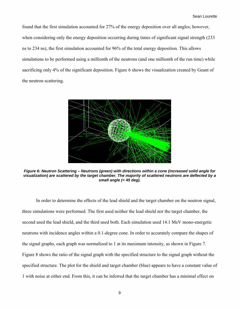
Sean Lourette
found that the first simulation accounted for 27% of the energy deposition over all angles; however,
when considering only the energy deposition occurring during times of significant signal strength (233
ns to 234 ns), the first simulation accounted for 96% of the total energy deposition. This allows
simulations to be performed using a millionth of the neutrons (and one millionth of the run time) while
sacrificing only 4% of the significant deposition. Figure 6 shows the visualization created by Geant of
the neutron scattering.
Figure 6: Neutron Scattering – Neutrons (green) with directions within a cone (increased solid angle for visualization) are scattered by the target chamber. The majority of scattered neutrons are deflected by a
small angle (< 45 deg).
In order to determine the effects of the lead shield and the target chamber on the neutron signal,
three simulations were performed. The first used neither the lead shield nor the target chamber, the
second used the lead shield, and the third used both. Each simulation used 14.1 MeV mono-energetic
neutrons with incidence angles within a 0.1-degree cone. In order to accurately compare the shapes of
the signal graphs, each graph was normalized to 1 at its maximum intensity, as shown in Figure 7.
Figure 8 shows the ratio of the signal graph with the specified structure to the signal graph without the
specified structure. The plot for the shield and target chamber (blue) appears to have a constant value of
1 with noise at either end. From this, it can be inferred that the target chamber has a minimal effect on
9

Sean Lourette
the signal from neutrons with incidence angles within a 0.1-degree cone. The lead shield (green)
appears to have a greater effect on the background signal. Although 4% of the neutrons that have
incidence angles outside the 0.1-degree cone hit the detector between 233 ns and 234 ns, a significantly
smaller percentage hit the detector between times of 233.5 ns and 233.8 ns. It can be presumed that this
will not significantly alter the neutron time of flight spread. The effect of the lead shield and the target
chamber on the FWHM from neutrons with incidence angles within the 0.1-degree cone is less than
1%.
Figure 7: Relative signal strengths for Figure 8: Ratios of signal strengths from 14.1 MeV neutrons in a 1-cm Figure 8. detector passing through various materials.
5. Conclusion
A Monte-Carlo simulation program was used to simulate neutron interactions in order to
understand the effects of the target chamber and lead shield on the detected neutron signal. The neutron
signal can be used to determine the initial velocities of the reacting ions or the temperatures required
10

Sean Lourette
for fusion. It was determined that the lead shield creates more neutron background than the target
chamber creates for 14.1 MeV neutrons with initial velocities within a 0.1-degree cone. It was also
determined that neither structure significantly alters (< 1%) the full width at half maximum (FWHM)
duration of the signal.
6. Acknowledgements
I would like to thank my advisor Dr. Christian Stoeckl for his support and guidance, which
made this project possible. I would also like to thank Dr. Orlin Gotchev for teaching me how to set up
and use Geant. Finally, I would like to thank Dr. Stephen Craxton, who made this entire experience
possible by accepting me into the High School Summer Research Program.
7. References
[1] Los Alamos National Laboratory, Physics Division Progress Report, Page 70 (1995)
[2] Bicron Newbury, Newbury, OH 44065-9577
[3] Wide-Dynamic-Range “Neutron Bang Time” Detector on OMEGA, LLE Review Volume 88,
Page 171 (2001)
[4] Geant, http://cern.ch/geant4
[5] Laboratory for High Energy Physics, University of Bern, Switzerland
[6] Dick Lerche, private communication (1997)
11

Precision Flash Lamp Current Measurement—Thermal Sensitivity
and Analytic Compensation Techniques
Ben Matthews
Precision Flash Lamp Current Measurement –Thermal Sensitivity and Analytic Compensation Techniques
2006 Summer Research Program
By Ben Matthews Advisors: Greg Brent, David Lonobile
Abstract:
For multiple-beam direct-drive laser fusion to occur it is essential that each laser beam hits the target with the same force. To help achieve this, the pump power provided to the flash lamps within the laser amplifiers is precisely monitored using a waveform digitizer module (WDM) designed at the University of Rochester’s Laboratory for Laser Energetics (LLE). Temperature changes within the WDM induce errors. In order to measure and reduce these errors a test stand has been constructed to accurately and automatically measure the effects of temperature on the digitizer. The test results provide a basis for the development of an analytic temperature compensation code for the WDM’s onboard FPGA (Field Programmable Gate Array), which is expected to greatly improve the accuracy of pump power readings at varying temperatures.
Page 1 of 7
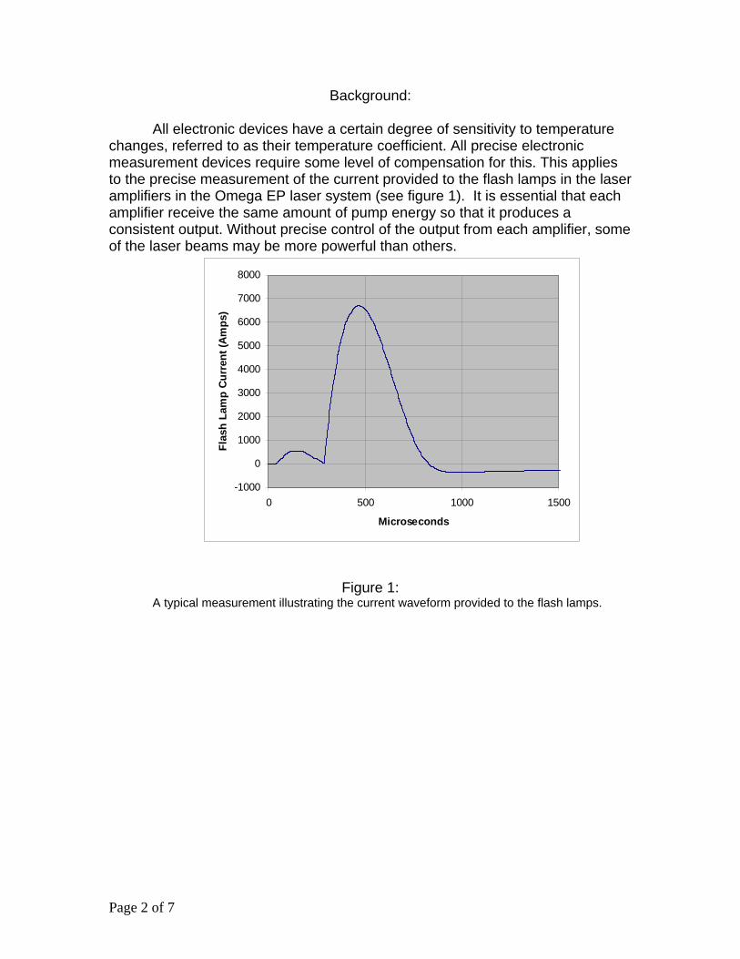
Background:
All electronic devices have a certain degree of sensitivity to temperature changes, referred to as their temperature coefficient. All precise electronic measurement devices require some level of compensation for this. This applies to the precise measurement of the current provided to the flash lamps in the laser amplifiers in the Omega EP laser system (see figure 1). It is essential that each amplifier receive the same amount of pump energy so that it produces a consistent output. Without precise control of the output from each amplifier, some of the laser beams may be more powerful than others.
-1000
0
1000
2000
3000
4000
5000
6000
7000
8000
0 500 1000 1500
Microseconds
Flas
h La
mp
Cur
rent
(Am
ps)
Figure 1:
A typical measurement illustrating the current waveform provided to the flash lamps.
Page 2 of 7

The waveform digitizer module, or WDM (see figure 2), is the device that
measures the current waveform provided by the power conditioning units (PCU’s) to the flash lamps. This device comprises seventeen, fourteen-bit analog-to-digital converters which are controlled by a field-programmable gate array (FPGA). These analog-to-digital converters measure the voltage collected by current sense transformers on the flash lamp power cables in order to determine the current being supplied. The FPGA processes and records the data being collected to the memory. This data is then collected by a single board computer for later analysis. The WDM was designed to contribute no more than a 1% error in the flash lamp waveform current measurement.
Figure 2: The waveform digitizer module (WDM) is used to digitize and store measurements of the current
provided to the laser amplifiers from the power conditioning units.
Page 3 of 7

Procedure
In order to characterize and compensate the WDM for temperature changes, a test stand is needed. To develop a test stand a few major components are required: a way to regulate temperature, a test waveform, and a way of analyzing the result. In order to efficiently characterize the WDM the process also has to be automated since a large number of boards need to be tested. The centerpiece of the test stand is a PC104 single board computer, of the same type that controls the WDMs installed in the laser system. This computer runs custom code, written in C as part of this research project, which controls the entire test without user intervention. To regulate the ambient temperature the WDM under test is placed in an environmental chamber and connected to an amplified arbitrary waveform generator output which simulates the PCU signals. The PC104 computer sets the environmental chamber to the desired temperature through an RS-232 (serial) connection. After the WDM has had time to reach thermal equilibrium, data is automatically collected from both a control WDM at room temperature and the WDM in the chamber. The arbitrary waveform generator is then turned off and the process is repeated at another temperature. The software also takes into account a correction factor to correct for environmental chamber errors. This factor was calculated early in the test stand development using a LabView program and sensors similar to those used on the WDM which were mounted throughout the chamber. In order to accurately find the effect that temperature has on the WDM it is tested at a wide range of temperatures, from about 10°C to about 70°C. It takes approximately 24 hours to test a single WDM throughout the full range of temperatures. In order to maximize the amount of thermal characterization data being collected the test waveform is a collection of sine waves with varying frequencies and amplitudes which emulate most of the possible input signals a WDM could be expected to measure. To help troubleshoot any problems that might occur, the test stand has some built-in debugging features. While running, the PC104 computer acquires a screenshot of an oscilloscope connected to the test stand. The oscilloscope triggers off the same trigger controlling the WDMs and test waveform generator and provides an image of both the trigger and the test waveform at each side of the test waveform amplifier. While the program is running it also displays some diagnostic information on the display of the PC104 such as the current, temperature and data storage file being written.
Page 4 of 7
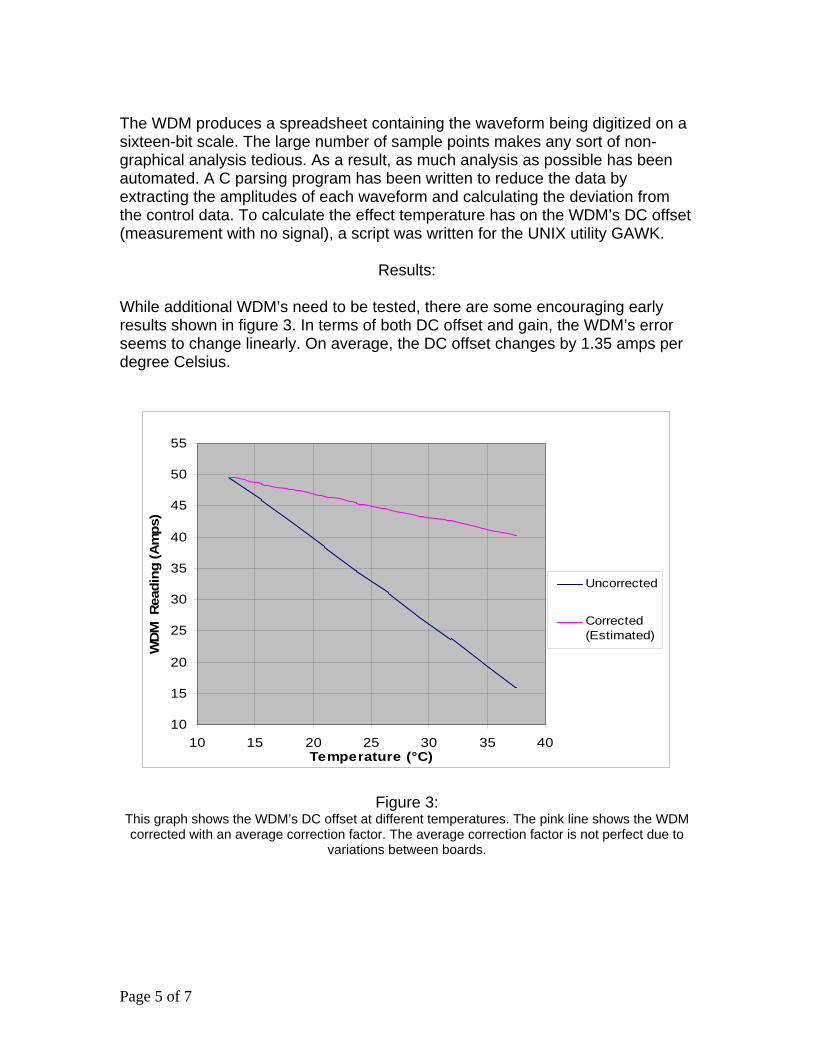
The WDM produces a spreadsheet containing the waveform being digitized on a sixteen-bit scale. The large number of sample points makes any sort of non-graphical analysis tedious. As a result, as much analysis as possible has been automated. A C parsing program has been written to reduce the data by extracting the amplitudes of each waveform and calculating the deviation from the control data. To calculate the effect temperature has on the WDM’s DC offset (measurement with no signal), a script was written for the UNIX utility GAWK.
Results:
While additional WDM’s need to be tested, there are some encouraging early results shown in figure 3. In terms of both DC offset and gain, the WDM’s error seems to change linearly. On average, the DC offset changes by 1.35 amps per degree Celsius.
10
15
20
25
30
35
40
45
50
55
10 15 20 25 30 35 40Temperature (°C)
WD
M R
eadi
ng (A
mps
)
Uncorrected
Corrected(Estimated)
Figure 3:
This graph shows the WDM’s DC offset at different temperatures. The pink line shows the WDM corrected with an average correction factor. The average correction factor is not perfect due to
variations between boards.
Page 5 of 7
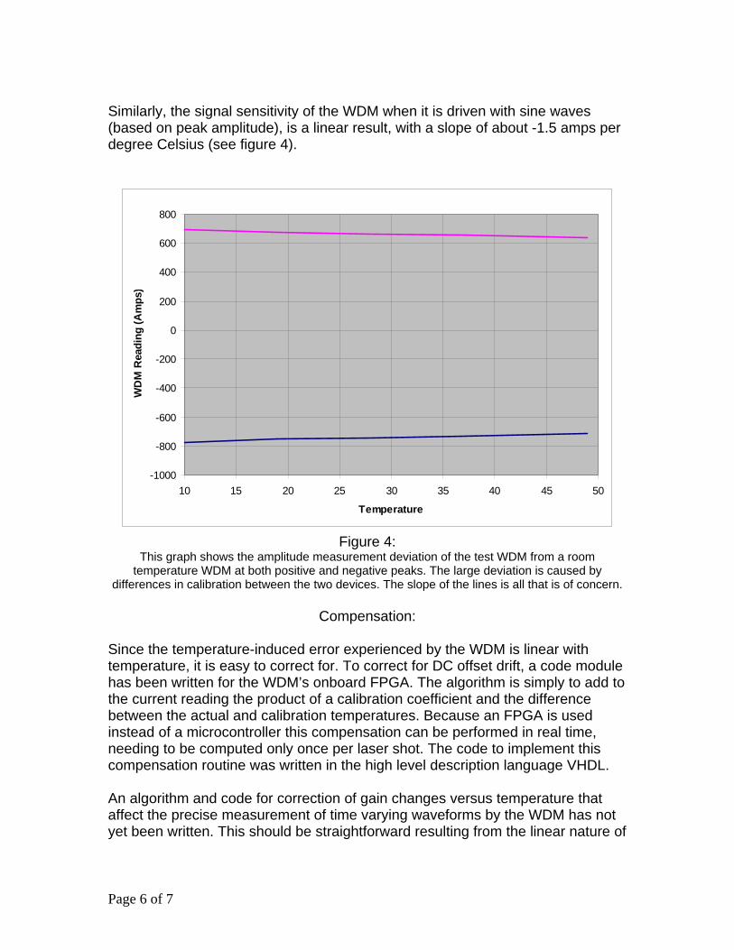
Similarly, the signal sensitivity of the WDM when it is driven with sine waves (based on peak amplitude), is a linear result, with a slope of about -1.5 amps per degree Celsius (see figure 4).
-1000
-800
-600
-400
-200
0
200
400
600
800
10 15 20 25 30 35 40 45 50
Temperature
WD
M R
eadi
ng (A
mps
)
Figure 4: This graph shows the amplitude measurement deviation of the test WDM from a room
temperature WDM at both positive and negative peaks. The large deviation is caused by differences in calibration between the two devices. The slope of the lines is all that is of concern.
Compensation:
Since the temperature-induced error experienced by the WDM is linear with temperature, it is easy to correct for. To correct for DC offset drift, a code module has been written for the WDM’s onboard FPGA. The algorithm is simply to add to the current reading the product of a calibration coefficient and the difference between the actual and calibration temperatures. Because an FPGA is used instead of a microcontroller this compensation can be performed in real time, needing to be computed only once per laser shot. The code to implement this compensation routine was written in the high level description language VHDL. An algorithm and code for correction of gain changes versus temperature that affect the precise measurement of time varying waveforms by the WDM has not yet been written. This should be straightforward resulting from the linear nature of
Page 6 of 7

this thermal effect on the WDM. This will likely be a C program run by the PC104 PCU control computer to post-process the data coming from the WDM. The WDM assemblies tested as part of this project seem to behave similarly with respect to thermal dependence. However the number of boards sampled is small, making it difficult to know whether a single compensation constant can be used or whether it will be necessary to test and compensate each board individually. If it turns out that each board must be compensated individually, it is possible to compute a correction factor for each board and store it in the PCU control PC104 computer’s storage for correction during post-processing after laser shots.
Discussion:
Prior to the start of this project, the effect that temperature would have on the WDM was uncharacterized. The WDM is required to have no more than 1% error, making its thermal characterization of great importance. While the temperature in the capacitor bays, where the WDMs are located, rarely changes more than a few degrees, the WDMs can not be calibrated in place. The room where they are calibrated may be at a different temperature. Thus characterization and compensation of the WDM thermal effects is required. Thermal effect correction also has the potential to reduce the thermal stabilization time required for the WDMs to be within specification. Even though the error caused by temperature turned out to be only a fraction of a percent as determined in this project, it combines with other factors increasing the total error. As a result, it is important that the WDMs be characterized and compensated for any temperature effects that may occur.
Conclusion:
The waveform digitizer, or WDM, is a highly precise current measurement device. It is absolutely necessary that the flash lamp current measured by the WDM is accurate in order to achieve uniform laser energy and pressure on the target. One factor contributing to errors in the WDM measurements is the effect of temperature. In this project it was determined that the DC offset linearly drifts with temperature by as much as 1.3 amps per degree Celsius in addition to the 1.5 amps per degree Celsius of drift measured on a time varying waveform. As a result, it is important to take temperature effects into account, either as data is being collected or in post processing. A compensation routine was successfully written to correct DC offset drift in collected data within the WDM FPGA.
Page 7 of 7

Evaluation of Confocal Microscopy for Measurement of the Roughness
of Deuterium Ice
Ryan Menezes
Ryan Menezes
1
Evaluation of Confocal Microscopy
for Measurement of the Roughness of Deuterium Ice
Ryan Menezes
Webster Schroeder High School
Webster, NY
Advisor: Dr. David Harding
Senior Scientist
Laboratory for Laser Energetics
University of Rochester
Rochester, NY

Ryan Menezes
2
Abstract:
In the direct-drive inertial fusion energy (IFE) concept, fusion targets at around 18 K are
rapidly injected into a chamber filled with low-pressure Xe gas at temperatures over 3000 K. In
experiments being carried out on OMEGA under the inertial confinement fusion (ICF) program,
similar targets are exposed to room temperature conditions prior to being irradiated. Because it is
necessary (for both IFE and ICF) that the deuterium (or deuterium-tritium) ice shell within each
target remains uniform until implosion, studies characterizing damage to the layer of deuterium
fuel are underway. One of these studies plans to use confocal microscopy to obtain 3-
dimensional images of the ice before and during heating. In preparation for cryogenic
measurements, a confocal microscope has been set up at room temperature to evaluate
parameters needed for this study. Several image degradations (arcs, noise, and reflection) have
been identified and investigated, and the scan parameters (image size, measurements per second,
measurements per pixel, and filter settings) have been optimized for the image clarity of a 40-
second scan. These parameters are required for future experiments.
1. Introduction:
In the future, fusion reactions could potentially yield clean and inexpensive electricity.
The production of this energy would occur when deuterium (2H) and tritium (3H) react to form a
helium atom and a neutron containing 14.1 MeV of energy (4He + 1n) [1]. For the energy in the
neutrons to be harnessed to run steam-powered turbines in a profitable power plant, the
deuterium and tritium fuel must be contained in targets which can be quickly and rapidly heated
and compressed to the intense conditions required for fusion. One method that could achieve
these conditions is direct-drive laser-induced inertial confinement fusion (ICF), under which

Ryan Menezes
3
fusion targets are (in the case of direct-drive) uniformly and directly irradiated with a short laser
pulse.
ICF targets contain deuterium vapor within a shell of deuterium
ice. (Tritium, which is radioactive, is not usually used in experiments.)
Fig. 1 presents the structure of the targets used in OMEGA experiments
at the University of Rochester Laboratory for Laser Energetics. The
solid deuterium fuel helps achieve the high densities needed for fusion.
The targets must be cryogenic, since hydrogen freezes at temperatures
below 20 K. Fig. 2 shows that, in comparison to ICF targets, inertial
fusion energy (IFE) targets (which are designed for use in power plant
situations) are larger and more complex. The ice shells in both targets
must remain uniform until implosion, or hydrodynamic instabilities will
prevent the target from properly imploding [2].
Both ICF and IFE target designs are subjected to heat fluxes
(indicated by the symbol Q in Figs. 1 and 2). ICF targets, which are
initially protected by heat shrouds, are exposed to room temperature for
0.05 to 6.0 seconds after the shrouds are removed, and before irradiation
[3]. IFE targets, which are shot into the chamber (not placed in it), have
a thin palladium layer that reduces blackbody radiation absorbed in the
target to insignificant levels. IFE targets experience heat flux from
collisions with xenon gas, which protects the chamber walls from the
energy created by fusion reactions [4]. The xenon gas is at low
pressures, but at very high temperatures (over 3000 °C). In both ICF and
Figure 1: Schematic of a cryogenic target currently used on OMEGA
Figure 2: Schematic of a cryogenic target used for inertial fusion
energy, injected at 400 m/s through 50 mtorr of Xenon
Figure 3: Diagram of buckling in heated Deuterium ice

Ryan Menezes
4
IFE designs, the heat striking the outside of the target spreads inward, causing the deuterium ice
to expand, bend, and buckle (see Fig. 3). It is necessary to understand this buckling in order to
create and maintain smooth fusion targets.
Because it is difficult to image the interior of
actual targets, a cryogenic setup was earlier designed
to simulate heat flow and buckling. Fig. 4 is a
schematic of this setup. The entire system is in a
vacuum chamber, allowing for control of
temperature and pressure. Within the vacuum
chamber is a smaller cell, which contains 160 torr of
deuterium gas and a confocal microscope (CFM)
positioned to image the window at the front of the
cell. This window should be cooled to 18.7 K, while
the rest of the cell, including the microscope, should
reach 91 K. Since the saturated vapor pressure of
deuterium gas is 160 torr at 18.7 K, the deuterium
condenses and freezes onto the back surface of the
window, and not on the rest of the cell or on the
microscope, which it could damage. Under the planned future experiment, a jet of hot xenon gas
heats the front of the window. Simultaneously, the microscope images the back surface of the ice
before and during buckling. A photograph of the smaller cell is shown in Fig. 5.
Figure 4: Schematic of the confocal microscope (light blue) within the experimental setup
Figure 5: Photograph of the smaller cell of the experimental setup
2. Confocal Microscope:
Fig. 6 illustrates the principle of confocal microscopy. A focused laser beam (red)

Ryan Menezes illuminates a small point on the sample. The reflected light (green) travels back through the lens.
All of the light passing through the lens that originates from the point on
the sample enters the end of the optical fiber, while any out-of-focus
light does not enter the optical fiber. A detector then measures the in-
focus light. (The strength of this signal corresponds to the height of the
point on the sample directly below the fiber.) Fig. 7 is a photograph of
the microscope that will be used in the planned experiment. The
piezoelectric scanner, which can be seen at the bottom of the
microscope stack, is a key component of the microscope. Instead of
using the scanner to move the sample under the objective, as is
traditionally done, this microscope moves the objective over the sample.
The scanner's customized placement makes this possible. Fig. 8 shows
the scan pattern used by the software that controls the scanner.
Directions sent to the scanner cause it to image a line (purple), then
image the same line, backward (red), and then step up to the next line
(pink) before repeating the process. Note that each of the line scans is
composed of steps as small as those between lines, and that readings
are taken after each step. After the scan, the scanning software takes
the data from the forward lines and combines them to create a forward
image, and does the same with the backward lines.
Figure 6: Diagram of the principle of confocal microscopy
Scanner Objective
Optical fiber
Coarse Positioners
Figure 7: Photograph of the confocal microscope
5 Figure 8: Diagram of the microscope’s scan pattern

Ryan Menezes
6
Basic operation of the microscope comprises 3 steps:
1. Using an oscilloscope, bring the microscope into the focal plane.
In addition to the scanner, the microscope stack contains three
piezoelectric motors for coarse positioning of the objective (see Fig. 7).
These motors move in the x, y, and z directions. To find the focal plane,
the z motor brings the objective close to the sample (less than 2 mm
away). Then, the laser is turned on. The detector sends the return signal to
the computer as a voltage, which can be measured using an oscilloscope
program. After this program is running, the z motor slowly takes the
objective farther away. The voltage return shows a sharp peak at the focal
plane, which is approximately 2.9 mm away from the objective.
2. Set the scanning parameters
Fig. 9 shows a screenshot of AttoScan, the
program used to set the scanning parameters
and take the image. AttoScan allows the user to
change several parameters:
- Pixels (Side Length) (Range: 1 to 10,000)
Figure 9: AttoScan screenshot
- Maximum Voltage (Range: 0 to 4) 1
- Scan Rate (measurements / s) (Range: 1 to 50,000) 2
- Average Rate (measurements / pixel)
There is also an option to run the current traveling to the scanner through a
low-pass filter with a cutoff frequency of 16, 160, or 1600 Hz.
1 These voltages are amplified 15 times before delivery to the scanner, as are all other voltage values identified. 2 The CFM manual was unclear. Within this project, the upper bound was considered to be 5,000.

Ryan Menezes
7
3. Begin the scan
Multiple scans can now be taken without interruption.
3. Experimental Results:
40µm
Figure 10: CFM image of a standardized copper grid
The microscope was set up at room temperature for test
scans and to identify appropriate scanning parameters. Images were
initially taken to illustrate functionality, and to verify the specified
scan size of approximately 40 micrometers. Fig. 11 shows images of
a piece of copper which was polished with sandpaper, using
perpendicular strokes. The diagonal lines, which probably did not result from mechanical effects
or from noise, illustrate the functionality of the CFM. Fig. 10 is an image of a copper grid whose
dimensions are known. The holes are ~30 micrometers across, while the bars are ~10
micrometers thick. This image verified the specified scan size of approximately 40 micrometers.
Figure 11: CFM image of a polished copper piece

Ryan Menezes
8
Figure 12: Dimensions of the AFM standard
40
Figure 15: Multiple CFM scans showing that the symmetrical
image is not a real feature
In order to evaluate image quality, standardized scans of an
atomic force microscopy (AFM) standard were taken. Fig. 12 illustrates
the pattern on this standard and its dimensions. The pitch is 10 µm, and
the depth of the pattern is 200 nm. Preliminary scans with this pattern
showed several types of image degradation (arcs, “reflection,” and noise).
In Fig. 13, arc-like distortions are observed, especially on the right side of
the image. In Fig. 14, a
“reflection” effect is observed on
the left side of the image. In Fig.
15, three images were taken of a
piece of plastic with small
perturbations to show that the
reflection is not a real feature. Between each scan, the objective was
moved to the left over the sample. As the symmetrical feature in Fig.
15 moves toward the center of the scan area, it becomes evident that
it is not actually symmetrical. The reflection effect most probably
results from a time lag in the scanning software, which causes the
software to add part of the backward image onto the forward image,
and part of the forward image onto the backward image. Fig. 16
provides evidence of this explanation.
40µm
40µm
Figure 14: CFM image with the “reflection” effect
Figure 13: CFM image with arc-like distortions
The final type of image degradation is observed in Fig. 17,
which shows noise in the signal to the detector. Instability in the laser
is believed to cause this effect. This belief is based on two facts: First,

Ryan Menezes
Figure 16: Actual and intended CFM images for forward and backward scans
the noise in Fig. 17 stops approximately three quarters
of the way through the scan, so the scanning
parameters are not responsible for the effect; and
Second, as Fig. 18 shows, wide and transient variation
occurs in the return signal even when no adjustments
are made. Nevertheless, there is a possibility that the
noise is caused by uncontrolled vibrations.
40 µm
Figure 17: CFM image with noise that stops partway through the scan
The AFM standard shown in Fig. 12 was
scanned many times to determine how different scan
parameters affect the image. Figure 18: Variation in the CFM’s return signal
a) Filter
(16, 160, or 1600 Hz)
Figure 19: CFM images showing the result of changing the frequency of the filter
Fig. 19 shows that lowering the
frequency of the filter reduces
the arc effect, while raising the
frequency reduces the
reflection effect.
9
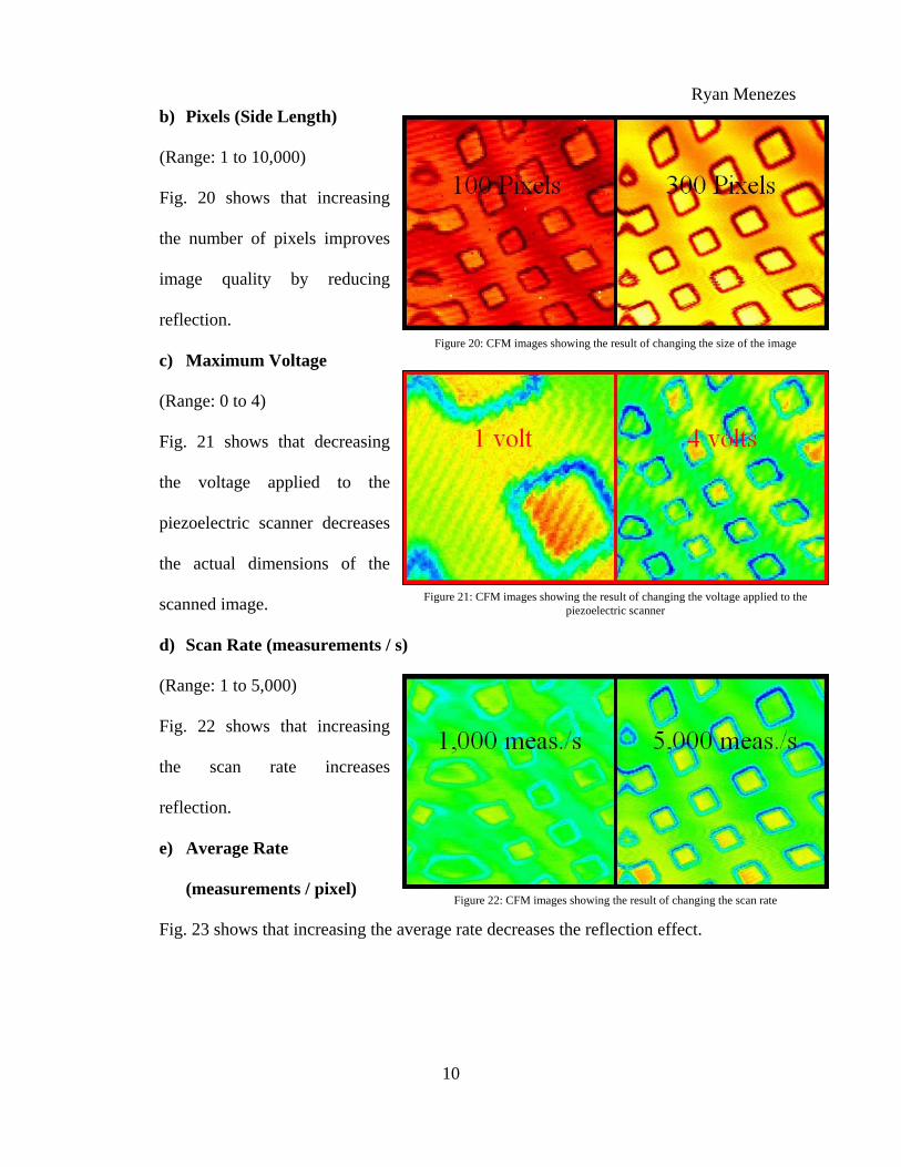
Ryan Menezes
10
b) Pixels (Side Length)
Figure 20: CFM images showing the result of changing the size of the image
(Range: 1 to 10,000)
Fig. 20 shows that increasing
the number of pixels improves
image quality by reducing
reflection.
c) Maximum Voltage
(Range: 0 to 4)
Fig. 21 shows that decreasing
the voltage applied to the
piezoelectric scanner decreases
the actual dimensions of the
scanned image. Figure 21: CFM images showing the result of changing the voltage applied to the piezoelectric scanner
d) Scan Rate (measurements / s)
(Range: 1 to 5,000)
Figure 22: CFM images showing the result of changing the scan rate
Fig. 22 shows that increasing
the scan rate increases
reflection.
e) Average Rate
(measurements / pixel)
Fig. 23 shows that increasing the average rate decreases the reflection effect.

Ryan Menezes
11
Figure 23: CFM images showing the result of changing the average rate
The time needed to scan an image is given by:
Time = (meas. per pixel) * (pixels per side)2 / (meas. per s)
or, Time = Average Rate * Pixels2 / Scan Rate
Since the microscope takes two images per scan (forward and backward), the time must be set to
20 seconds to optimize parameters for a 40-second scan. (The scanning software takes ~8
seconds to prepare before beginning the scan. This added time was ignored.) Based on earlier
scans, 100 was determined to be the lowest value for Pixels that still preserved image quality.
(Increasing Pixels above 100 increases scanning time quickly because time varies directly with
the square of side length.) Under these conditions,
20 = Average Rate * 100 * 100 / Scan Rate,
so Average Rate / Scan Rate = 1 / 500.
The images in Fig. 24 show that the best
image results from the highest average rate,
even though this increases the scan rate as
well.
Figure 24: CFM images showing the result of simultaneously changing the scan rate and the average rate

Ryan Menezes
12
4. Summary:
The effects of different parameters, evident in Figs. 17 through 24 and in other scanned images,
are summarized in Fig. 25.
Figure 25: Summary of results
It was also found that the voltage applied to the piezoelectric scanner, while affecting the scan
size, has no noticeable effect on the image quality.
4. Conclusion:
The confocal microscope can demonstrably image a 40 by 40 micrometer area every 40
seconds. The optimal scanning parameters for this time goal are:
Pixels (Side Length) = 100
Maximum Voltage = 4
Filter = 16 Hz
Scan Rate = 5,000 measurements / s
Average Rate = 10 measurements / s
The microscope is now ready to be incorporated into the cryogenic setup. The 40-second

Ryan Menezes
13
scan parameters will be used in the experiment, and the heat flow will be adjusted to
accommodate image size and resolution. However, many factors will change at cryogenic
temperatures. At low temperatures, more voltage must be applied to the piezoelectric scanner for
it to move the same distance, but higher voltages can be applied without causing damage (up to
10 V before amplification). Also, if the noise observed in Fig. 17 is due to vibration, it may
disappear at cryogenic temperatures.
Two possibilities which should be explored in the future are the possibility of increasing
the Scan Rate past 5,000 (and increasing the Average Rate proportionally) and of replacing the
16 Hz filter with the 1600 Hz filter combined with a computed low-pass filter. Both of these may
result in better image quality.

Ryan Menezes
14
5. Acknowledgements:
Dr. R. Stephen Craxton, without whose invitation I would not have had the opportunity to
participate in this program.
Dr. David Harding, who helped me obtain samples to image and whose advice and
encouragement improved the project and this report.
Ms Mariana Bobeica, who designed and built the cryogenic setup and who will carry out the
planned experiment.
References
[1] V.N. Goncharov, Basic Principles of Direct Drive Ignition Target Design, LLE Review Vol.
106, p. 83 (2006).
[2] R.W. Petzoldt, Direct Drive Target Survival During Injection in an Inertial Fusion Power
Plant, Nuclear Fusion Vol. 42, p. 1 (2002).
[3] D. Harding, private communication (2007).
[4] D.T. Goodin, et al., Developing Target Injection and Tracking for Inertial Fusion Energy
Power Plants, Nuclear Fusion Vol. 41, p. 527 (2001).

Computational Modeling of Spectral Properties of Nickel Dithiolene Dyes
Rui Wang

Rui Wang
Computational Modeling of Spectral Properties of Nickel Dithiolene Dyes
Rui Wang
Fairport High School Fairport, NY
Advisor: Kenneth Marshall
Laboratory for Laser Energetics University of Rochester
Rochester, NY
November 2006

Rui Wang
Abstract
Nickel dithiolene dyes, noted for their intense long-wavelength electronic transitions,
have been notoriously dificult molecules to model. This study has investigated the use of time-
dependent density functional theory (TDDFT) to model these dyes. The absorption spectra of an
extensive set of near-infrared nickel dithiolene dyes have been evaluated for the first time using
TDDFT. Bulk solvent effects have also been accounted for. Excellent agreement between
theoretical and experimental maximum absorption wavelengths has demonstrated the high
accuracy of TDDFT. Successful prediction of the physical properties of proposed nickel
dithiolene dyes leads to informed selection of candidates for future synthesis, significantly
reducing the time and cost of materials development. Calculations for new nickel dithiolene dyes
predict that the addition of sulfur atoms to the side chains will increase the maximum absorption
wavelength by up to 160 nrn. These results can aid in the further development of nickel
dithiolene dyes in applications including near-infrared lasers, telecommunications, and sensor
protection.
1. Introduction
Nickel dithiolenes were first synthesized in the 1960s and were noted for their intense
absorption over a broad range of near-infrared (IR) wavelengths. These organometallic dyes
contain a zerovalent planar core with dithiolene rings surrounding a nickel atom (Figure 1).
Figure 1. Structure of nickel dithiolene dye molecules. Different dyes are formed by
substitutions of the R groups.
Nickel dithiolene dyes have characteristics that can be useful in an array of applications.
Their intense long wavelength absorption is a result of the low-energy 7c-7c* transition between

Rui Wang
the highest occupied molecular orbital (HOMO) and the lowest unoccupied molecular orbital
(LUMO)'. In addition, this class of dyes exhibits an auxochromic shift (shift in absorption
spectra) depending on the R groups attached2. This property makes nickel dithiolenes useful as
near-IR dyes for optical applications. The zerovalent nature of the dithiolene core imparts
relatively high solubility in nonpolar solvents, including liquid crystal hosts, and makes these
dyes useful for near-IR liquid crystal device applications3. Some metal dithiolenes have an
inherent liquid crystal phase4 and thus can be dissolved in a liquid crystal host in relatively large
quantities without changing the characteristics of the host fluid.
Transition-metal dithiolenes are of interest for many applications. First, the inherent
solubility and stability of these materials lead to their use in photodetectors5, which are used by
the fiber-optic telecommunications market as components that detect laser light in fiber-optic
systems and transform that light into electrical current. The primary wavelengths of interest for
this application are 1300 nm and 1550 nm. They can be used for both long-haul transport and
telecommunications receiver systems carrying high-speed voice and damnternet traffic5.
Second, nickel dithiolene dyes are used in Q-switching saturable absorbers to produce short
intense pulses for IR lasers because of their high thermal and optical ~tability.~ A dye with an
absorption maximum near the laser wavelength will absorb the laser radiation and the electrons
of the dye molecules will be boosted into the excited state as the energy level in the lasing
medium increases. When the dye is optically "saturated" (most of the dye molecules are in the
excited state) the dye no longer absorbs the laser radiation and a short, intense laser pulse is
released. These lasers generally operate at wavelengths between 950 and 1100 nm. Third,
because nickel dithiolenes absorb in the near-IR range, they are of interest for IR sensor
protection for the military. For this application, the electronic absorption band is tunable from

Rui Wang
around 600 nm to 1600 nm by changing either the dye structure (through synthesis), or the helical
pitch length of the dye (if it is chiral).) The Air Force is currently investigating the application of
transition metal dithiolenes absorbing in the 700-900 nrn region as part of a liquid crystal electro-
optical device for night vision and avionics applications.)
The synthesis of nickel dithiolenes is a multi-step, low-yield process and is thus costly
and time-consuming. Conventional trial-and-error synthesis approaches result in the need to
synthesize a large number of compounds to establish physical properties trends. As has been
previously demonstrated in the pharmaceutical industry, computational chemistry can be used to
predict the most promising materials for synthesis, thus resulting in substantial savings in time,
resources, and cost.
Although computational methods are well established for organic compounds, very little
work has been done in modeling the electron interactions in transition metal organometallic
molecules. The most recent attempt at computing the structures and properties of nickel
dithiolene dyes was performed by C. Lauterbach and J. ~ a b i a n . ~ Because of computational
limitations and data availability, only a few nickel dithiolene molecules were modeled using an
older method known as single configuration interaction CIS).^ More recently, D. Jacquemin et
a1.8. 97 l o predicted the optical properties of other classes of organic dyes such as indigo and nitro-
diphenylarnine derivatives using a newer method known as time dependent density fhctional
theory (TDDFT)' ' . Their methodology produced relatively high computational accuracy for
absorption spectra calculations. Thus, TDDFT seems a promising solution to the computational
difficulties of nickel dithiolenes, which are also optical dyes.
In this study, the computational approach of TDDFT has been applied for the first time to
predict the absorption spectra of nickel dithiolene systems. The maximum absorption

Rui Wang
wavelengths have been accurately predicted for a large number of nickel dithiolene dyes and four
new dyes have been proposed that extend the maximum absorption wavelength further into the
IR. This improved computational method can lead to advances not only in near-IR devices, but
also in applications of optical dyes across the electromagnetic spectrum.
2. Previous Research
There are three common methods for excited state computation: (1) semiempirical and
Zerner's Intermediate Neglect of Differential Overlap (ZIND0);12 (2) Hartree-Fock and single
configuration interaction CIS);^ and (3) density functional theory (DFT) and time-dependent
density functional theory (TDDFT).'
The first calculations of nickel dithiolene properties used the early semiempirical
13, 14 quantum chemical models. These models save computational time by using experimental
data to fit the calculation according to known parameters. Using approximations, this method
decreases the computational time but at the cost of accuracy. ZINDO is one type of semi-
empirical algorithm for studying excited state and spectroscopic properties of molecules. This
method is limited in accuracy, as all semiempirical models are, by the degree of similarity
between the molecule being studied and known molecules from which parameters are taken.
In the Hartree-Fock method, all nuclei are assumed motionless with respect to the
electrons, electron orbitals are expressed as one-electron functions centered on each atom, and
the multi-electron calculation of the model is assumed to be given by the sum of all single-
electron calculations of the molecule.15 Relativistic effects and electron correlation effects
(electron-electron interactions) are mostly neglected. The Hartree-Fock method becomes
decreasingly accurate with increasing molecular size.15 This method is used for approximating
the ground state energy of a molecular system. Post-Hartree-Fock methods have been developed

Rui Wang
to improve on the Hartree-Fock method by approximating the electron correlation of a system.16
This gives more accurate results but at a greater computational cost. The single configuration
interaction (CIS) is one example of a post-Hartree-Fock method limited to single excitations.
This method is expanded fiom the Hartree-Fock calculations to incorporate electronic excitation
and changing shell levels. However, known results using this method indicate that its accuracy is
not high for larger molecules. 15, 17
Previous work done on modeling nickel dithiolene dyes by Lauterbach and Fabian
utilized the CIS method for excited-state absorption spectra calculation^.^ Their study calculated
the structure, electron distribution, electron bonding, and spectral properties of transition-metal
molecules including nickel dithiolenes. Other transition metal compounds investigated included
metal diiminolenes, dioxylenes, and diselenolenes utilizing nickel, palladium, and platinum as
the central metal. Lauterbach and Fabian performed all calculations in the gas phase and thus
omitted all effects associated with the solvents that host the dyes during experimental
measurements of the absorption spectrum. Their analysis of the structure focused mostly on the
effect of substitutions for the nickel and sulfur atoms in Figure 1.
More recently, density functional theory has emerged as a useful computational method
for ground state properties. Unlike the Hartree-Fock method, DFT uses the electron density as the
foundation of its calculations instead of the many-electron wavef~nction.'~ The main advantage
is that the wavefunction, a complex function in multi-dimensional space that takes into account
individual electrons, is replaced by a density function in three spatial dimensions, which greatly
lowers the computational cost. DFT has been extended to time-dependent density functional
theory (TDDFT), which models the evolution of the system in time in response to an external
disturbance, as described below. Jacquemin used TDDFT extensively to model the absorption
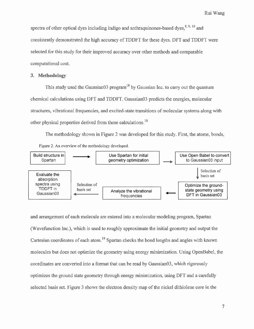
Rui Wang
8,9, 10 spectra of other optical dyes including indigo and anthraquinones-based dyes, and
consistently demonstrated the high accuracy of TDDFT for these dyes. DFT and TDDFT were
selected for this study for their improved accuracy over other methods and comparable
computational cost.
3. Methodology
This study used the Gaussian03 program'8 by Gaussian Inc. to carry out the quantum
chemical calculations using DFT and TDDFT. Gaussian03 predicts the energies, molecular
structures, vibrational frequencies, and excited-state transitions of molecular systems along with
other physical properties derived from these calculation^.'^
The methodology shown in Figure 2 was developed for this study. First, the atoms, bonds,
Figure 2. An overview of the methodology developed.
Spartan
absorption spectra using Selection of
TDDFT in basis set Gaussian03 - frequencies
+ to Gaussian03 input
1 Selection of basis set
and arrangement of each molecule are entered into a molecular modeling program, Spartan
(Wavefunction Inc.), which is used to roughly approximate the initial geometry and output the
Cartesian coordinates of each atom.19 Spartan checks the bond lengths and angles with known
molecules but does not optimize the geometry using energy minimization. Using OpenBabel, the
coordinates are converted into a format that can be read by Gaussian03, which rigorously
optimizes the ground state geometry through energy minimization, using DFT and a carefully
selected basis set. Figure 3 shows the electron density map of the nickel dithiolene core in the

Rui Wang
ground state calculated by Gaussian03.
Basis sets play an important role in these calculations. The electron density function of
the given molecule is calculated using a linear combination of spatially dependent elementary
functions contained in the basis sets. The potential function is calculated as the sum of the
external potential (interactions with ions), the Hartree potential (classical electron-electron
interactions), and the "exchange-correlation" potential (complex many-body effects that have to
be approximated).20 The basic concept of DFT is to vary the coefficients in the basis functions
Figure 3. The ground-state electron density of the nickel
dithiolene core (R=H).
and the coordinates of all the ions until a
stationary point with minimum energy is
found. The geometry at the point of the
energy minimum is given as the optimized
geometry. The choice of basis sets is important because enough functions are needed to give
sufficient accuracy, yet too many or inappropriate functions may cause convergence problems
that result in the program failing to find the lowest-energy minimum.
The vibrational spectrum is then analyzed to check the computed geometry, since the
accuracy of the absorption spectra depends on the accuracy of the structure. The substantial
computational time for the larger molecules leads to the omission of this step unless an anomaly
in the absorption maximum warrants investigation of the vibrational frequencies.
Finally, the transition energy to the excited state is calculated using TDDFT. TDDFT
disturbs the ground state density calculated by DFT by applying an impulse potential. This
impulse potential contains all frequencies so that the frequency-dependent time evolution of the
electron density allows the absorption spectrum and the wavelength of maximum absorption to
be ca l c~ la t ed .~~
Rui Wang
Since all reported experimental maximum absorption wavelengths of nickel dithiolene
dyes were measured in solution, solvent effects are taken inlo account for both DFT and TDDFT
calculations. The potential function is adjusted for the presence of solvents using the polarizable
continuum model (PCM).~' The PCM divides the calculation into a solute part (the nickel
dithiolene molecule) and a solvent part (the surrounding solvent molecules), which is
characterized by its dielectric constant, radius and other macro-scale properties.
4. Optimization Of Basis Sets
4.1 Basis Sets For Energy Minimization
To evaluate the density function using Gaussian03, the exchange-correlation portion oi
the potential function was approximated using the hybrid functional PBElPBE (25% electron-
exchange and 75% electron-~orrelation).~~ This was done for both DFT and TDDFT calculations.
It was important to choose an appropriate basis set. A large number of basis sets are
commonly used, which are clarified with standard notation. For instance, in 6-3 1 l++G(d, p), '6-
31 1' indicates 11 functions (6+3+1+1) for the s-orbital and 5 functions (3+1+1) for the p-orbital
in large atoms, and 5 functions (3+1+1) for the s-orbital in hydrogen, while G denotes this as a
Gaussian basis set. The notation I++' indicates the addition of "double diffuse" functions
(designed to model more accurately electrons farther fiom the nucleus of an atom) for all atoms;
single diffuse, '+', treats only nonhydrogen atoms. The notation '(d, p)' indicates the addition of
"polarization" functions (describing more orbitals, in this case one function for the d-orbital in
larger atoms and one function for the p-orbital in hydrogen).23 Eighty-one Gaussian basis sets,
with combinations of polarization and diffuse functions supplementing the basic 6-3 1 1 G set,
were systematically analyzed with the nickel dithiolene core (R = H in Figure 1). The
polarization functions, which aid in the modeling of bonding interactions, ranged from (d, p) to

Rui Wang
(3df, 3pd). Each polarization function variation was evaluated with double difise, single difise,
and no difise functions. The core structure was chosen for this study because it is the part of the
overall nickel dithiolene molecule that affects the absorption spectra the most.24 Because no
extensive R groups are attached, the computational time was relatively short (-30 minutes). If a
basis set failed to converge on the nickel dithiolene core, it was avoided for calculations of
structures with R groups attached. This problem was sometimes encountered for relatively large
basis sets. For each optimized geometry derived from a specific basis set, measurements were
taken and compared with experimental values25 for the bond lengths of Ni-S, S-C, and C-C, and
for the bond angles of S-Ni-S, Ni-S-C, and S-C-C of the nickel core. The error is reported in
Figure 4 as a percentage error averaged over all measurements for each basis set. The errors for
all basis sets are graphed with groups of double, single, and no diffuse functions. Larger basis
sets generally require greater computational time because more polarization functions are used.
The results in Figure 4 are arranged from the most extended to the least extended basis sets so
that the trade-off between accuracy and computational time can be assessed. Because the
Figure 4. Mean absolute error of selected bond lengths and angles using various basis sets, which are labeled by polarization and diffuse functions. (Double and single difhse errors overlap.) The star indicates the chosen basis set.
Heavy atoms: tdf, 3df. 3df, 3df. 3df. 3df. 2df. 2df, 2df, 2df, 2df. 2df, df, df, df, df, df, df, 36. 3d. 36 , Pd 24 . 2d . d , d , d H~drogenatoms: 3pd 2pd pd 3p 2p p 3pd 2pd pd 3p 2p p 3pd 2pd pd 3p 2p p 3p 2p p 3p 2p p 3p 2p p
Basis-set polarization function
Rui Wang
difference in accuracy between double and single diffuse functions is minimal, it was determined
that adding double diffuse functions is not necessary. The underlying assumption for this choice
was that hydrogen does not play a significant role in the modeling of these compounds. The line
graphs for the basis sets with diffuse functions follow a general trend upward in percent error as
smaller basis sets are used. In Figure 4, the polarization functions for the heavy atoms seem to
affect the error more than the polarization functions for hydrogen atoms. This observation is also
true for basis sets without diffuse functions, though more fluctuation occurs.
Recognizing that even with the fluctuations shown on the graph, the difference between
the highest point and the lowest point on the entire graph is only an error of 0.38%, the goal was
to find the least time-consuming basis set with a reasonably small error. The focus is on the right
side of the graph with relatively small basis sets since convergence problems sometimes arise
with the larger basis sets and the addition of more polarization hc t i ons does not seem to
produce better results. Therefore, the basis set 6-3 1 1G(3d, 2p) (star on the graph) was chosen for
the geometry optimization since it produced a local minimum in error for a reasonable
computational time. In the previous study by Lauterbach and ~ a b i a n , ~ though the list of
molecules investigated was more extensive than in previous studies, the experimental absorption
maximum value cited was for the nickel dithiolene with H as each of the four R groups. This
compound thus provides the only useful error comparison between this study and theirs. Table 1
compares the structural data from this study and data obtained by Lauterbach and Fabian along
with the experimental data. The average error obtained by Lauterbach and Fabian, 1.77%, is
higher than the 1.3 1% error obtained here.

Rui Wang
Table 1. Comparison between theoretical and experimental bond lengths [A] and angles ["I Bond lengths: Experimental ["I This work [bl Lauterbach and Fabian
Ni(1)-S( 1) 2.100 2.123 2.178 s ( l)-c( 1) 1.687 1.685 1.705 c ( 1 )-c(2) 1.353 1.372 1.374
Bond angles: S(1)-Ni(1)-S(2) 88.5 92.5 92.1 Ni(1)-S(1)-C(1) 107.8 103.5 102.9 S(2)-C(2)-C(l) 117.9 120.2 121.1
Average % Error 1.3 1% 1.77% [a] Ref. 25 - [b] Calculated using 6-3 1 1G(3d, 2p) - [c] Ref. 6 Calculated using 6-3 1 1+G*
The choice of basis set in these calculations was verified by computing the vibrational
frequencies using the chosen basis set, 6-3 1 1 G(3d, 2p). Using DFT, Gaussian03 computes force
constants and the resulting vibrational frequencies of the molecule, along with the intensities at
those frequencies.'* The major frequencies, (799 cm-I and 1132 cm-I for C=S bonds; 1399 cm-I
for the C=C bond; and around 3 175 cm-' for C-H bonds) all agreed with experimental
confirming the accuracy of both the molecular structure and the computed absorption spectra.
When the procedure developed for the nickel dithiolene core was applied to larger nickel
dithiolene dye molecules using DFT, the basis set 6-3 1 1 G(3d, 2p) was found to produce
convergence errors and the computational time increased dramatically. The basis sets may have
been too restricting, and often no stationary energy minimum could be found within
computational limits. Several smaller basis sets were then tested, and 6-3 1 1 G(d, p) was found to
satisfactorily produce the geometry optimization.
4.2 Basis Sets For Time-Dependent Absorption Wavelength Calculations
The next step is the excited state, time-dependent calculations. Figure 5 shows the
electron density shift in the nickel dithiolene core when the molecule transitions from the ground
state (HOMO) to the excited state (LUMO). The blue area indicates the most electron-rich
region, while the red area indicates the electron-deficient region. The electron density shifts from

Rui Wang
Figure 5. Electron density maps of the electronic transition modeled by TDDFT for the nickel core (Figure 1). Blue indicates high electron density.
(a) Highest Occupied Molecular Orbital (HOMO)
Transition - (b) Lowest Unoccupied Molecular Orbital (LUMO)
the center of the molecule to the four s u l h ligands during this energy transition.
A new basis set was needed, as the TDDFT calculations differ fiom the geometry
calculations. First, TDDFT calculations were performed using basis sets without diffuse
functions, but the errors in the resulting absorption spectra were not acceptable and the focus
turned to basis sets with single-diffuse functions. Therefore, a systematic test was run in which
all the single-diffuse basis sets were used to calculate the absorption spectra of the core, holding
the optimized structure constant (Figure 6). The graph again demonstrates that the polarization
functions for heavy atoms are more important in determining the errors in the calculation. From
the global minimum of this graph, the 6-3 1 l+G(d, 2p) basis set was chosen for the TDDFT
calculations of all the remaining nickel dithiolene dyes under investigation.
Figure 6. Error in the absorption-maximum photon energy of the nickel dithiolene core using different single diffuse (+) basis sets for the excited state calculations. The ground-state geometry was optimized using the 6-3 1 1G(3d, 2p) basis set.
Basis-set polarization function (heavy, hydrogen)

Rui Wang
5. Determination of Maximum Absorption Wavelengths
The main purpose of this study was to investigate the accuracy of TDDFT in predicting
the maximum absorption wavelengths A,,,, of various nickel dithiolene dyes. The computed A,,,,
for all investigated nickel dithiolene dyes are reported in Table 2 along with experimental data.
The graph in Figure 7(a) provides a comparison of the theoretical A,,,, with experimental results.
The electron energy transition responsible for producing these maximum absorption wavelengths
was between the ground state and the first excited state (see Figure 5), which confirms both
25,27 experimental and previous computational findings. Only systems with solvents that are
parameterized in Gaussian03 were selected so that a fair comparison could be performed. The
computational time for each molecule on eight processors running on a 1.6 GHz Itanium I1 SGI
Altix supercomputer ranged from hours to days, depending on the complexity of the structure
and the properties of the solvent.
As a measure of accuracy, the maximum absorption wavelength calculated for the nickel
dithiolene core in this study was compared with that of a previous study.6 The absorption
wavelength is 678.92 nm, an error of 0.10 eV (all errors are compared in eV for consistency and
convention) from the experimental value of 720 n n 2 This result is a substantial improvement
from the previous result of 623 nrn determined with the CIS method6 (an error of 0.27 eV).
Since TDDFT is to be used as a predictive tool for determining the maximum absorption
wavelength of optical dyes, the data collected in this study was statistically treated to provide a
more direct prediction of experimental values. It is clear from Figure 7(a) that the raw
wavelengths calculated here consistently underestimate the experimental values. Such data are
usually subjected to statistical treatment lo using simple linear regression. The data plotted in
Figure 7(a) were fit with the equation: I,,,,, ,,,. = 64.84 + 1.0021 A,,,,, theory, with a Pearson

Rui Wang Table 2. Comparison between raw theoretical, statistically treated theoretical, and experimental L, for various nickel dithiolene dyes. All absorption maxima are calculated using 6-31 1 +G(d, 2p).
R-Groups Solvent Theory (raw) Theory (treated) Experiment Ref.
R1, R4 R2, R3 (nm) h m a x (nm) Lax (nm) H H Hexane 678.9* 745.7* 720 2
Methyl Methyl Chloroform 704.3 771.2 774 2 Methyl Methyl Dichloromethane 702.7 769.6 770 28
Butylthio Butylthio Acetone 893.4 961 .O 1002 4 Butylthio Butylthio Chloroform 900.7 968.3 1004 2 Phenyl Phenyl Chloroform 809.9 877.2 866 2
2-Napthyl 2-Napthyl Chloroform 852.2 919.7 905 2 H Phenyl Dichloromethane 774.8 841.9 810 28
Ethyl Ethyl Dichloromethane 680.2 747.0 770 28 Phenyl Methyl Dichloromethane 731.7 798.7 795 28 Phenyl Ethyl Dichloromethane 719.0 786.0 795 28 Phenyl Phenyl Dichloromethane 81 1.9 878.4 865 28
4-octylphenyl H Dichloromethane 776.3 843.5 865 28 4-octylphenyl H Hexane 764.8 832.0 850 2
4-bromophenyl 4-bromophenyl Dichloromethane 830.9 898.2 870 28 4-methylphenyl 4-methylphenyl Dichloromethane 854.1 921.6 900 28
Pentylthio Pentylthio Acetone 905.2 972.9 1002 4 2-thienyl 2-thienyl Chloroform 957.4 1025.3 982 2
*This geometry was calculated using 6-31 1 G(3d, 2p). The geometry for all other structures was calculated using 6-31 IG(d,p).
Theoretical h a x (nm)
800 900 1000
Theoretical A,, (nm)
(b)
Figure 7. (a) Comparison between the raw theoretical k and the experimental I.,,,=. The line shows linear regression. (b) Comparison between the statistically treated theoretical k and the experimental A,,,=. The line indicates L a x , theory = L a x . exp.
Rui Wang
correlation coefficient R~ of 0.921. All the raw values were then adjusted using this equation,
giving the treated theoretical wavelengths of Figure 7(b), which can then be used to improve the
theoretical predictions.
These predictions of the maximum absorption wavelength of the nickel dithiolene core
are the most accurate to date. For the entire group of nickel dithiolene dyes investigated, the
mean unsigned error is 0.033 eV. This translates to an absolute difference of 20.8 nm between
experimental values and treated theoretical values on average. These errors are much smaller
than previously reported errors; even studies using TDDFT typically report errors ranging from
0.2 to 0.4 eV for transition-metal molecules. 29,30
The trends among various nickel dithiolene dyes are correctly modeled. The structures
with terminal groups containing sulfur or phenyl rings are found to have longer-wavelength
absorption maxima. The solvatochromatic effects (solvent effects on the A,,,,) are also reasonably
predicted. For the structure R1& = 4-octylphenyl and R2R3 = H, the experimental values show a
hypsochromic shift (blue shift) of 15 nrn, when the solvent changes from dichloromethane to
hexane, while the theoretical values give a shift of 1 1.5 nrn. Similarly, the solvatochromatic
effects on the nickel dithiolene dye with R = methyl and the dye with R = butylthio are modeled
accurately. These fbrther demonstrate the validity of TDDFT for the quantitative evaluation of
the maximum absorption wavelength of various nickel dithiolene dyes.
With the accuracy of the methodology validated, several new nickel dithiolene dyes were
designed and modeled using DFT and TDDFT in an attempt to extend the measured absorption
wavelength into the IR. Since sulfur seems to effect a bathochromic shift (red shift) when
included as part of the R groups, and sulfur-containing structures have traditionally been more
soluble than phenyl-containing structures3' (which also effect a bathochromic shift), the new

Rui Wang
dyes were designed with sulfur added to the R groups. The results shown in Table 3 confirm this
hypothesis in each of three groups, with significant red shifts in the maximum absorption
wavelength of up to 160 nm. It is anticipated that this work will allow more nickel dithiolene
dyes to be synthesized with maximum absorption wavelengths further into the infrared region.
Table 3. Comparison of newly designed nickel dithiolene structures (in bold) and similar existing dyes.
RI R4 R2R3 Solvent Predicted Am,
(nm) E ~ P . Am, (nm) 4-phenyl-Br 4-phenyl-Br DiChloroMethane 895.2 870
SBr SBr DiChloroMethane 975.2 - SF SF DiChloroMethane 971.6 -
Methyl Methyl Chloroform 772.0 774 S-methyl S-methyl Acetone 845.8 -
H H Hexane 745.7 720 SH SH Hexane 907.5 -
The absorption spectra of an extensive set of nickel dithiolene dyes have been studied
using TDDFT to compute excited state energies, with bulk solvent effects taken into account. A
hybrid functional and two basis set combinations, 6-3 1 1 G(d, p) for the ground state geometry and
6-3 1 l+G(d, 2p) for the excited state energies, were used in this study. Close agreement between
the theoretical and experimental h, has been achieved for 18 known dyes, with a mean absolute
error limited to 0.033 eV. A methodology has been used for nickel dithiolene dyes that can be
adapted to future studies of these and other optical dyes.
This study provides a significant step forward in advancing the science of computational
chemistry in organometallics, especially shown by the low error in this study as compared with
those currently reported in the literature. Four new nickel dithiolene molecules have been
designed and modeled, with findings that indicate that adding sulfur to the R groups will increase
the h, by up to 160 nrn. Future work will seek to extend the l,,,, further into the infrared
region, by making additional modifications to the terminal R groups. The success of this method

Rui Wang
will greatly assist the development and synthesis of new transition metal dithiolenes and will aid
in the use of nickel dithiolenes as near-IR dyes in applications such as telecommunications,
sensor protection, and liquid crystal devices in laser systems.
Acknowledgements
I would like to thank my advisor Mr. Kenneth Marshall for his guidance and support in
my research, as well as Dr. R Stephen Craxton for not only providing the opportunity to work at
the University of Rochester's Laboratory for Laser Energetics but also helping me during the
final stage of my project. In addition, I would like to thank Anthony Noto for mentoring me on
the applications and limitations of the Gaussian03 program.
References
1. Mueller-Westerhoff, U. T.; Vance, B. Dithiolenes and Related Species. In Comprehensive Coordination Chemistry; Wilkinson, G., Gillard, R. D., McCleverty, J. A., Eds.; Pergamon: Oxford, 1987; Vol. 2, pp 595-63 1.
2. Mueller-Westerhoff, U. T.; Vance, B.; Yoon, D. I. Tetrahedron 1991,47,909-932.
3. Marshall, K. L.; Schudel, B.; Lippa, I. A. Proc. SPIE 2003,521 3,20 1-2 12.
4. Marshall, K. L.; Klehn, B.; Watson, B.; Griffin, D. W. Proc. SPIE 2003,5188,48-60.
5. Caironi, M.; Natali, D.; Sampietro, M.; Ward, M.; Meacham, A. P.; Devillanova, F. A.; Arca, M.; Denotti, C. Proc. SPIE 2004,5464, 165- 175.
6 . Lauterbach, C.; Fabian, J. Eur. J Inorg. Chem. 1999,11, 1995-2004.
7. Stanton, J. F.; Gauss, J.; Ishikawa, N.; Head-Gordon, M. J Chem. Phys. 1995,103,4160- 4174.
8. Jacquemin, D.; Preat, J.; Wathelet, V.; Perpete, E. A. J Chem. Phys. 2006,124,0741 04.
9. Jacquemin, D.; Preat, J.; Charlot, M.; Wathelet, V.; Andrk, J.; Perpete, E. A. J Chem. Phys. 2004, 12 1 (4), 1736- 1743.

Rui Wang
10. Perpkte, E. A.; Wathelet, V.; Preat, J.; Lambert, C.; Jacquemin, D. J. Chem. Theory Comput. 2006,2,434-440.
1 1. Runge, E.; Gross, E. K. U. Phys. Rev. Lett. 1984,52,997-1000.
12. M.C. Zerner, ZINDO, A Semiempirical Quantum Chemistry Program, Quantum Theory Project, University of Florida, Gainesville, FL, 1996.
13. Schrauzer, G. N.; Mayweg, V. P. J Am. Chem. Soc. 1965,87,3585-3592.
14. Schrauzer, G. N. Acc. Chem. Res. 1969,2,72-80.
15. Corsello, S. Student Research Reports, 1998 Summer Research Program for High School Juniors at the University of Rochester's Laboratory for Laser Energetics, 1998.
16. Hehre, W. J. Ab Initio Molecular Orbital Theory 1986 (Wiley, New York).
17. Jacquemin, D., private communication, 2006.
18. Frisch, M.J. et al., Gaussian03, Gaussian, Inc., Pittsburgh, PA, 2004.
19. SPARTAN '04, Wavefunction, Inc., 18401 Von Karman Ave., #370, Irvine, CA 92715,2003.
20. Marques, M. A. L.; Gross, E. K. U. Annu. Rev. Phys. Chem. 2004,55,427-455.
21. Arnovilli, C.; Barone, V.; Carnmi, R.; Cancks, E.; Cossi, M.; Mennucci, B.; Pomelli, C. S.; Tomasi, J. Adv. Quantum Chem. 1998,32,227.
22. J. P. Perdew, K. Burke, and M. Emzerhof, Phys. Rev. Lett. 1996, 77,3865.
23. Ahlrichs, R.; Taylor, P. R. J. Chem. Phys. 1981, 78,3 15-324.
24. Eisenberg, R. Prog. Inorg. Chem. 1970,12,295-369.
25. Herman, Z. S.; Kirchner, R. F.; Loew, G. H.; Mueller-Westerhoff, U. T.; Nazzal, A.; Zerner, M. Inorg. Chem. 1982,21,46-56.
26. Schlapfer, C. W.; Nakamoto, K. Inorg. Chem. 1975,14, 1338-1344.
27. Hill, C. A. S.; Charlton, A,; Underhill, A. E.; Malik, K. M. A.; Hursthouse, M. B.; Karaulov, A. I.; Oliver, S. N.; Kershaw, S. V. J. Chem. Soc. Dalton Trans. 1995,4,587-594.
28. Winter, C. S.; Oliver, S. N.; Manning, R. J.; Rush, J. D.; Hill, C. A. S.; Underhill, A. E. J. Mater. Chem. 1992,2,443-447.

Rui Wang
29. Petit, L.; Makdivi, P.; Adamo, C. J. Chem. Theory Comput. 2005,1,953-962.
30. Adamo, C.; Barone, V. Theor. Chem. Acc. 2000,105,169- 172.
31. Marshall, K. L., Painter, G. Lotito, IS., Noto, A.G., Chang, P., Mol. Cryst. Liq. Cryst. 2006, 454,47[449] - 79 [481].

Dynamic Energy Grouping in Multigroup Radiation Transport Calculations
Nicholas Whiting
1
Dynamic Energy Grouping in Multigroup Radiation Transport
Calculations
Nick Whiting
Bloomfield High School
Advisor: Dr. Reuben Epstein
University of Rochester
Laboratory for Laser Energetics
2006 Summer High School Research Program
Abstract
During an OMEGA inertial confinement fusion (ICF) implosion, some of the
absorbed laser energy is reemitted by the shell of the target as thermal radiation. In order
to simulate the radiative heating of the core of the target and other radiative effects,
numerical models of radiation transport are included in ICF simulation codes. These
models typically divide the radiation spectrum into many energy groups. Unfortunately,
these simulations can take a long time to run if the radiation transport calculation is
repeated for each of a large number (e.g. 40) of energy groups. A new strategy for
reducing the number of groups has been evaluated using a simple radiation program. A
common technique for reducing the time needed for the radiation simulation is to regroup
a large number of energy groups into fewer, larger groups in a way that avoids too great a
loss of precision. The novel feature of the new strategy is adjust the boundaries of these
few energy groups automatically at regular time intervals, each time optimizing the
resolution of the spectrum, thus improving the accuracy of the calculations without
significantly lengthening the processing time. My program, based on an earlier version
by Brian MacPherson,1 has been used to develop and analyze this method for radiation
transport test cases. I will show results demonstrating this method and how it can
compensate for the inaccuracies due to the reduced spectral resolution of four-group
calculations.

2
1-Introduction
The numerical simulation of hydrodynamics is very important at the Laboratory
for Laser Energetics in designing ICF experiments and in testing our understanding of the
outcomes of these experiments. At the moment, these simulations may take hours, or
even days, to complete. This long simulation time stems from the complexity and
number of the arithmetic operations that must be completed to simulate the
hydrodynamics of laser-driven implosions, including the transport of radiation through
the target material. These calculations involve collecting all possible photon energies
(hν) into some number of intervals or “groups,” and perform the transport calculation on
each of these groups. This number of groups is usually 48, 12, or 4 in the simulations
used at LLE. The accuracy and time required for calculation are directly related to each
other. The time required in this simulation can be reduced by regrouping those photon
energy groups into a smaller number of groups.
This project worked with a model problem in which a 1 keV blackbody spectrum
was incident on a planar slab of material. The time evolution of the temperature profile
in the slab, which depends on radiation transport in the slab, was calculated. In the case
of the program I worked with, we chose to use 40 intervals and 4 regrouped intervals of
photon energy, which cut the time required to simulate the radiation transport by a
significant amount (ideally, a factor of 10). Unfortunately, this time-saving measure
loses accuracy when compared with its many-group counterpart due to the relative lack
of spectral resolution. A proposed remedy for this inaccuracy is “dynamic regrouping,”
in which this regrouping is repeated periodically over the course of the simulation so that
the boundaries of the four energy groups change, adapting to the radiation spectral energy
density at any given point in time. If this method works as intended, it would retain the
time-efficiency of static regrouping while retaining much of the accuracy of the many-
group calculations. In order to test this method, a program was written in 2005 by Brian
MacPherson.1 This program only took the method as far as “static regrouping,” where
the same 4 groups are kept fixed throughout the calculation. I wrote a dynamic
regrouping section of code into this program. I also addressed a number of problems
associated with the length of the time steps, the calculation of the new groupings, and
various other sections of the program. I processed my results using the PV Wave

Advantage programming environment.2
2-Method
2.1 Radiation Transport
In simulating radiation transport and demonstrating dynamic regrouping, the
program must calculate numerous properties and radiative effects experienced by the
material. The most important quantities are opacity κν, emissivity εν, intensity Iν,
radiation spectral energy density Uν, and matter temperature T. All energy quantities,
such as kT and hν are expressed in units of keV.
2.1.1 Opacity
Opacity is the material property that determines the rate at which the material
absorbs radiation. This may be dependent on a number of properties, such as the
temperature, density, and composition of the material, and also on the frequency (or
photon energy) of the incident radiation. In my program, I used simple opacity
expressions chosen by Fleck and Cummings3 for their standard test problems. The
opacity κν is equal to:
(1)
( )[ ],)1(27 1
3−
−−= cm
keVhe kTh
νκ
ν
ν
where (1-e-hν/kT) is a correction for stimulated emission. The subscript ν denotes photon
frequency or energy dependence. In this equation, the opacity is inversely related to the
cube of the photon energy, so higher-energy photons will penetrate farther into the slab.
This opacity is not strongly temperature dependent, but I did work with a strongly
temperature dependent opacity at one point,
( )[ ] ( )[ ],)1(27 1
3−
−−= cm
keVkTkeVhe kTh
νκ
ν
ν(2)
Here, the opacity is also inversely related to temperature kT. This program and these
opacity expressions are needed only for the analysis of the dynamic regrouping method,
and more complicated and quantitatively accurate representations of real material
3

opacities are not required.
2.1.2 Emissivity
Emissivity is the rate at which a material emits radiation. This rate is determined
by the properties of the material (temperature, composition, and density). For my
program, Kirchoff’s law was used for the calculation of emissivity:
).(TBνννε = κ (3)
This equation relates emissivity εν directly to opacity κν by the Planck function of
temperature Bν(T). In this program, the Planck function is:
( )[ ] .105.044)(322 ergkeVhTB ×
=νπ (4)
sec)1(e 2/kTh keVcm−νν
2.1.3 Intensity
As radiation travels through the slab, it is both absorbed and emitted. This
produces an intensity Iν of radiation, given by the equation of radiative transfer, where
dIν/ds, the rate of change of Iν with distance s along the propagation path, is:
.4 νν
νν κπ
ε Ids
dI−= (5)
In its calculation of intensity, the program uses the solution to Eq.5 giving the intensity
at any given distance s and for any given photon energy hν. The solution for a slab of
uniform opacity κν and emissivity εν for the intensity Iν(s) along a straight line path
starting from s=0, where Iν(0) = Iν0 is
.44
)( 0seIsI νκν
νν
ν πκε
πκε −
⎟⎟⎞
⎜⎜⎛
−+= (6) νν ⎠⎝
2.1.4 Radiation Energy Density
The radiation spectral energy density is the spatial density of radiation
energy within a unit range of photon energy at some distance s into the slab. The
4

radiation spectral energy density is given by:
.)(cos)(2)(1
1∫−= θπ νν dsIsU (7)
In this equation, the intensity values are integrated over all path angles θ, where θ
specifies the photon path direction relative to the slab normal direction θ = 0. This is to
account for radiation being emitted in all directions. The intensity is independent of the
azimuthal angle φ due to the planar symmetry of the problem. In calculating the intensity
over the full 180° range of θ, the program splits 180° into 16 segments of equal solid
angle. The radiation energy density is of particular importance in calculating and
understanding the matter temperature results.
2.1.5 Matter Temperature
The evolution of the matter temperature is dependent on the rate of energy
absorption determined by the opacity κν, the cooling rate determined by the emissivity
ε ν, and the intensity Iν of the radiation at that distance into the slab:
5
Here, CV is the specific heat of the material that is being simulated. In the test problems,
it is a constant set to , where a is the radiation energy density constant, 305917.0 aTCV =
4314101.37
keVcmerga ×= . The matter temperature equation gives two important terms:
the absorption rate and the emission rate. The absorption rate is given by the opacity
multiplied by the intensity Iν νκ integrated over all angles (2 cosd d )π θΩ =∫ ∫ and over
all photon energy values ( )d hν∫ . The emission rate is the emissivity of the material εν
integrated over all photon energy values hν. These values are used to find the matter
temperature after a finite time step Δt:
.)()(∫ ∫∫ ννν hdhddIdt
CV −Ω= νενκdT(8)
( )[ ].
)(1)(00 thdthddITCTT
V Δ−+ΔΩ+=
)(0 thdTCV Δ+ ∫∫∫∫ νεανκ ννν (9)
νεα ν

6
Eq.9 expresses the temperature T at the end of the time step as an “explicit,” “implicit,”
or intermediate solution of Eq.8, depending on the value of the parameter α being 0, 1, or
an intermediate value.3 When Eq.8 is solved explicitly (α = 0) for T, the T-dependent
terms on the right-hand side of Eq.8 are first written entirely in terms of the initial T
value, T0. The implicit solution (α = 1) is the opposite, in the sense that the right-hand
side of Eq.8 is first written in terms of the final value of T, which is T itself. The implicit
formulation of Eq.8, expressed as Eq.9 with α = 1, is used by the program to determine
the matter temperature.
2.2 Existing Simulation
At the Laboratory for Laser Energetics, two main hydrocodes are used. These are
the DRACO (2D hydrodynamics modeling) and LILAC (1D hydrodynamics modeling)
codes. These codes can calculate radiation transport by grouping all photon energy
values into a relatively large number of groups in order to preserve accuracy. This entails
a large number of calculations and is extremely time consuming. In handling the angle-
dependent aspect of radiation transport, the hydrocodes almost always use the diffusion
approximation, a more approximate method than we used in this program. Some effort
has been taken to shorten the time needed for these simulations to run by gathering
photon energy values into a smaller number of groups, but no automated dynamic
regrouping strategy has yet been implemented. These simulations are needed for the
researchers at the lab to simulate ICF implosions in order to better design experiments.
Reducing the amount of time necessary to run a simulation without losing a significant
amount of precision would prove extremely valuable to the researchers at the LLE.
2.3 Static Regrouping
Static regrouping was implemented by consolidating a large number of small
groups into a smaller number of larger groups that remain fixed throughout the
calculation. In my work, I used a test problem of Fleck and Cummings where a 4 cm-
thick slab is irradiated by a 1-keV blackbody spectrum. Figure 1 is a contour plot of the
spectral energy density of the slab of material at 50 ps (20 time steps). This is the point at
which the photon energy groups are first recalculated. Before this, the values are
collected into 40 photon energy groups, each of which was 0.25 keV wide. Then, these

7
groups are regrouped into 4 groups. The boundaries of these new groups are shown in
Fig. 1 as horizontal lines. After this, the calculation continues, using only these 4 groups.
An inaccuracy in the spectral energy density is caused by the relatively poor spectral
resolution resulting from using only 4 groups. The inaccuracy produced by the
regrouping remains throughout the course of the calculation and builds upon itself. The
time at which the many-group calculation is converted to the few-group calculation also
has a significant impact on the accuracy of the calculation. Also, the program represents
conditions at a finite number of distances into the slab. The slab is divided into 10 finite
distance intervals, as is done in the Fleck-Cummings test problems,3 giving only
quantities defined at ten spatial points throughout the slab. The program uses finite
difference integrations in time, distance, angle, and energy to handle these calculations.
2.4 Dynamic Regrouping
Dynamic regrouping was suggested4,1 as a possible solution to the difficulties
presented by static regrouping. This method involves the successive recalculation of the
boundaries of the four large groups at regular time intervals. This regrouping is repeated
periodically using spectral energy density values calculated with the same 40 groups used
in determining where the boundaries of the four large groups were to be placed in the first
regrouping. The simulation then continues for the following predetermined cycling time
interval using only the four new groups. Once the cycling time has expired, the
simulation goes on to perform yet another 40-group time step to produce a smooth
spectrum with a smoothness similar to that of the spectral energy density shown earlier in
Fig. 1. Then, a new set of 4-group boundaries is obtained from the smooth 40-group
spectral energy density, and the program cycles again. All of this is done automatically
by the program. Overall, this method of simulation improves upon the approximation of
a low-resolution 4-group spectral grid without adding a significant amount of calculation
time.
The contour plots of radiation spectral energy density produced during the
simulation provide a good illustration of dynamic regrouping. Originally, the spectral
energy density is smooth and accurate (Fig. 1). The contours of the 4-group spectrum
can be seen from the contour plots produced during the 4-group calculations, such as Fig.
2 and Fig. 3. These spectra are seen to be very approximate, due to the relatively poor

8
spectral resolution, compared with the smoothness of the spectra produced early in the
simulation. Figure 4 is an example of a spectral energy density produced from a 40-
group calculation later in the simulation (447.5 ps). This plot illustrates the point in the
dynamic regrouping cycle when the simulation returns to a more accurate representation
of the spectral energy density for one time step in order to allow new group boundaries to
be obtained for the 4-group time steps to be done next. This is the key detail in the
dynamic regouping cycle.
2.5 The Program
Dynamic regrouping has been incorporated into the radiation transfer program
originally written by Brian MacPherson.1 This program consists primarily of a time-
stepping loop where the length of the time step is controlled. In each time step, the
opacity and the emissivity are calculated for each of the 10 slab spatial zones. Then, the
program obtains the intensity by numerically integrating Eq.5 and then uses Eq.7 to
obtain the radiation energy density. The program goes on to calculate the change in
matter temperature with Eq.9, which is the solution to Eq.8. At the regrouping time, new
boundaries are calculated for the four large energy groups. Then, the program repeats
this process in the next regrouping cycle.
2.5.1 Opacity and Emissivity Calculations
The program uses Eq.1 and Eq.3 to calculate the opacity and emissivity,
respectively. Equation 2 was also used as an alternative temperature-dependent opacity
in another Fleck-Cummings test problem.3 The opacity and emissivity functions are
evaluated at each increment of distance into the material and at each of the 40 photon
energy values. These stored values are used later in the calculation of intensity and in the
calculation of the matter temperature. The emissivity and opacity are recalculated at
every time step.
2.5.2 Intensity and Radiation Energy Density
The program first calculates the intensity values at all distances s along each of
the 8 paths spaced equally in solid-angle intervals from 0° to 90°, relative to the forward
direction (θ=0°), away from the blackbody source, and for each photon energy value.

9
00 =νI
These integrations are initialized with Iν0 equal to the blackbody spectrum at T = 1 keV.
The program uses Eq.6 to perform the integration along s. The final intensity at the end
of each distance increment is used to evaluate the contribution to the absorption rate term
in Eq.9 for each distance step, for each photon energy, and for each angle. This
calculation is also performed in an identical fashion for the intensities along the
remaining 8 paths from 90° to 180°, except that each of these rays are initialized with
at the outer boundary. All these values of intensity are then used to determine
the radiation spectral energy density using Eq.7. These values of radiation energy density
can then be displayed in contour plots so that the radiation energy density can be
compared at different points in time. Figure 1 and Fig. 4 show plots of radiation energy
density at two different points in time. It can be seen that early in the simulation, higher
energy photons penetrate deeper into the material, but that later in the simulation the
distribution of low and high energy photons deep in the material is more even.
2.5.3 Matter Temperature
The matter temperature evolution is obtained from Eq.8 after calculating the
radiation absorption and emission rates. The opacity is multiplied by intensity and
integrated over all angles and all photon energies to give the absorption rate. The
emissivity is integrated over all photon energies to give the emission rate. The absorption
and emission rates are used in Eq.9 to find the matter temperature. The program solves
this equation implicitly, setting α equal to 1. Figure 5 is plotted with respect to distance
into the slab at one specific time (750 ps) in the simulation. Figure 6 is the temperature at
one distance into the slab (1.2 cm) over the entire time that the slab is exposed to the
incident 1 keV blackbody spectrum.
2.5.4 Regrouping
Regrouping is performed automatically after a certain number of time steps. This
number can be set to any value, but I chose to have it perform the first regrouping after
20 time steps (50 ps), and then regroup at intervals of 40 time steps (100 ps). In the
calculation of the new 4-group boundaries, the program uses the 40-group radiation
spectral energy density and places one boundary at the maximum of the spectral energy
density integrated over the whole volume, one boundary at each of the 50%-maximum

10
value points, and one boundary each at the lowest and highest photon energy values.
This regrouping reduces the number of calculations performed, but it also creates
radiation energy density contour plots that are more approximate due to the loss of
spectral resolution.
3-Results
3.1 Dynamic Regrouping vs. Static Regrouping
In the first 60 time steps (150 ps), through the end of the first dynamic regrouping
cycle, the dynamic and static regrouping results are the same, since both methods use the
same 4 groups during this time. Figure 6 shows this with the 40-group calculation as a
solid line, dynamic regrouping as a heavy-dotted line, and static regrouping as a light-
dotted line. The dynamic regrouping result deviates from the static regrouping result
after the 60th time step (150 ps). Immediately after this time step, the dynamic
regrouping performs a single 40-group calculation of the radiation spectral energy density
to use in determining a new set of 4-group boundaries. Since these 4 new groups allow
better resolution of the spectrum at this point in time, the temperature results begin to
more closely follow the results of a full 40-group calculation. This improvement is very
slight and is not clearly visible in Fig. 6 at this depth (1.2 cm) until after the next
regrouping cycle at the 100th step (250 ps). Figure 7 also illustrates these results,
showing the effects of dynamic regrouping on the temperature deeper (2.7 cm) into the
slab. Here, the dynamic regrouping results deviate visibly toward the 40-group results
after the second regrouping at the 60th time step (150 ps). This simulation also has
produced temperature profiles that are similar to those that were obtained in test problems
by Fleck and Cummings.3 Figure 5 is a good example of these temperature profiles, and
again shows improvement over static regrouping when dynamic regrouping is used. This
improvement is probably the most important result of my work.
3.2 Time step Variation
The size of the time step also had some effect on the accuracy of both static and
dynamic regrouping. If the time step was too large, the temperature profile errors at early
times could be excessive, as is illustrated by the example in Fig. 8. As the time step
comes closer and closer to zero, the accuracy of the results increases because the
11
difference equation becomes a better approximation of the differential equation. Figure 9
shows the accuracy produced by using a time step that is fairly small. Unfortunately,
with a significantly smaller time step, the time required to run the program increases by a
factor that is inversely related to that time step. I had to choose a time step that was small
enough to produce relatively accurate results, but that did not require an especially large
amount of time to compute. After experimenting with a few other values, I chose a 2.5 ps
time step as the most efficient. As can be seen from Figure 10, this time step still
provides improved accuracy over static regrouping, while at the same time not being too
small to undo the efficiencies gained by using regrouping. With any significant change
to the test-case problem (such as adding strongly temperature-dependent opacity), the
size of the time step may have to be adjusted to maintain accuracy. For example, a
strongly temperature-dependent opacity can greatly increase the heating rate, causing the
matter temperature values to jump up to many times the 1 keV source radiation
temperature if the time step is too large, which is physically impossible. In order to run
the calculation for the same amount of simulated time, the number of time steps
increases, and the computation time begins to become a problem once more. A different
method of calculation may allow for a larger time step to be taken, but at present, the
time step has a very large effect on the accuracy (and so, the usefulness) of dynamic
regrouping.
3.3 Boundary Variation
In the regrouping process, boundary values for the larger energy groupings are
chosen based on a calculation of the space-integrated spectral energy density.
Boundaries are placed at the highest and lowest photon energy values (10.0 keV and 0.25
keV in the case of this program). A boundary is also placed at the photon energy with the
highest spectral energy density. Then, two more boundaries are placed, each at the
photon energies with 50% of the maximum radiation energy density. This percentage
was chosen because it would distribute the energy in the groupings fairly evenly.
However, I experimented with varying this percentage, and found that different
percentages produced results with different accuracy. I determined this by comparing the
temperature profiles produced by static and dynamic regrouping with these percentage
changes to a full 40-group calculation and to the profiles produced by the default 50%

12
calculations (Fig.7). I raised the boundaries to 60% of the maximum, and found that
static regrouping lost accuracy (Fig.11), but that dynamic regrouping regained a small
amount of accuracy. I also lowered the boundaries to 40% of the maximum and found
that static regrouping gained accuracy and followed dynamic regrouping more closely.
Experimentation with the boundary selection strategy appears to benefit both the static
and dynamic regrouping results to some degree. The boundary calculations in this
regrouping strategy must be analyzed in more detail before any definite conclusions can
be drawn from the results, but, at the moment, this seems to be a step in the right
direction.
4-Conclusions/Future Work
In researching dynamic regrouping as an effective method for accurately and
efficiently simulating radiation transfer, I have found that the dynamic regrouping retains
the efficiency of static regrouping while, at the same time, more closely follows the
results of a full 40-group calculation. A nearly ten-fold improvement in time efficiency
was observed, as well as the improvement of accuracy, over that of static regrouping. I
have also found that adjusting the regrouping method affects the accuracy of results
produced by this program. By continuing to experiment with this strategy, the accuracy
of dynamic regrouping may be further improved. Among the adjustable aspects are the
time step length and the group boundary selection method. The time step appears to have
the greatest effect on the results obtained. If it is too small, efficiency is lost, but if it is
too big, accuracy is lost. The boundary calculations have a less drastic affect on the
accuracy of dynamic regrouping, but they appear to have a larger effect on the accuracy
of static regrouping. During further testing, this method will have to be exposed to many
more test problems to determine its potential benefits or limitations. At present, dynamic
regrouping has only been tested against one test problem. However, with much work
remaining to be done, dynamic regrouping still appears to be a promising method of
improving the efficiency of radiation transfer simulations.
5-References
[1] Brian MacPherson, “Dynamic Energy Grouping in Multigroup Radiation
Transport Calculations,” 2005 Summer Research Program for High School

13
Juniors, Student Research Reports LLE Laboratory Report #343.
[2] PV-Wave Advantage Programming Environment
[3] J. A. Fleck, Jr. and J. D. Cummings, “An implicit Monte Carlo scheme for
calculating time and frequency dependent nonlinear radiation transport,” Journal
of Computational Physics, vol. 8, pp. 313-342, 1971.
[4] R. Epstein, private communication, Jul-Aug. 2006.

Time = 50.0000e- 1 2 (set) 10.00 1 I I I I I
0.4 0.8 1.2 1.6 2.0 2.4 2.8 3.2 3.6 4.0 Distonce (cm)
Fig. 1 : Contour plot of the radiation spectral energy density as a function of distance into the slab and photon energy using 40 energy groups. 'The boundaries selected for the 4-group calculation in Fig.2 are shown as horizontal lines.
Time = 452.500e- 12 (set) 10.00 I I I I I I I
9.25 -
8.50 L 1
Time = 52.5000e- 12 10.00 I I I I I I I I I
I I
0.4 0.8 1.2 1.6 2.0 2.4 2.8 3.2 3.6 4.0 Distonce (cm)
Fig.?: Same as Fig. I , except that the radiation spectral energy density is calculated using only 4 groups.
Time = . . T 447.500e- 1 7 12
9.25 l O.OO r-- 1 I
0.4 0.8 1.2 1.6 2.0 2.4 2.8 3.2 3.6 4.0 0.4 0.8 1.2 1.6 2.0 2.4 2.8 3.2 3.6 4.0 Distonce (cm) Distonce (cm)
Fig.3: Same as Fig.2, but 160 time steps (400 ps) later. Fig.4: Same as Fig. I, but 159 time steps (397.5 ps) later when the smoother 40-group spectrum is obtained. This plot shows the deeper penetration of the lower energy photons than at earlier times in the simulation, such as is shown in Fig. 1 .
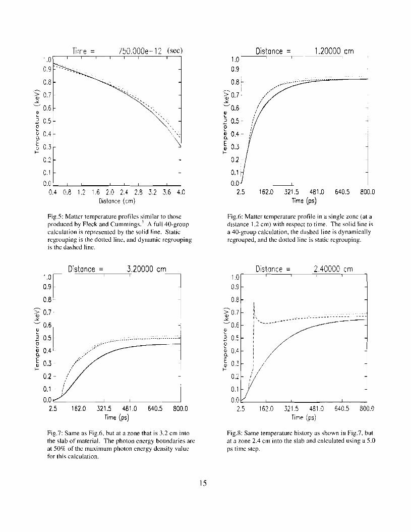
0.4 0.8 1.2 1.6 2.0 2.4 2.8 3.2 3.6 4.0 Distance (cm)
Fig.5: Matter temperature profiles similar to those produced by Fleck and ~ummings. ' A full 40-group calculation is represented by the solid line. Static regrouping is the dotted line, and dynamic regrouping is the dashed line.
2.5 162.0 321.5 481 .O 640.5 800.0 Time (ps)
Fig.7: Same as Fig.6. but at a zone that is 3.2 cm into the slab of material. The photon energy boundaries are at 50% of the maximum photon energy density value for this calculation.
Distance = 1.20000 cm 1 .o " I
2.5 162.0 321.5 481.0 640.5 800.0 Time (ps)
Fig.6: Matter temperature profile in a single zone (at a distance 1.2 cm) with respect to time. The solid line is a 40-group calculation, the dashed line is dynamically regrouped, and the dotted line is static regrouping.
Distance = 2.40000 cm
2.5 162.0 321.5 481 .O 640.5 800.0 Time (PS)
Fig.8: Same temperature history as shown in Fig.7, but at a zone 2.4 cm into the slab and calculated using a 5.0 ps time step.

Distance = 1 .o
0.0 2.5 162.0 321.5 481 .O 640.5 800.0
Time (ps)
Fig.9: Same as Fig.8. but calculated with a 1.25 ps time step.
Distance = 3.20000 cm ,
- - 7' -
0.9 i
2.5 162.0 321.5 481.0 640.5 800.0 Time (ps)
Fig. 1 1 : Same as Fig.7, except the photon energy boundaries were set at 60% of maximum photon energy density value for this calculation.
Distance = 2.40000 cm I .o 0 1
2.5 162.0 321.5 481 .O 640.5 800.0 Time (ps)
Fig. 10: Same as Fig.8, but calculated using a 2.5 ps time step.
2.5 162.0 321.5 481 .O 640.5 800.0 Time (ps)
Fig. 12: Same as Fig. 7, but the photon energy boundaries were set at 40% of maximum photon energy density value for this calculation.