1

20. Extinction Probability for Queuesand Martingales

(Refer to section 15.6 in text (Branching processes) for discussion on the extinction probability).

20.1 Extinction Probability for Queues:

• A customer arrives at an empty server and immediately goes for service initiating a busy period. During that service period, other customers may arrive and if so they wait for service. The server continues to be busy till the last waiting customer completes service which indicates the end of a busyperiod. An interesting question is whether the busy periods are bound to terminate at some point ? Are they ? PILLAI

2

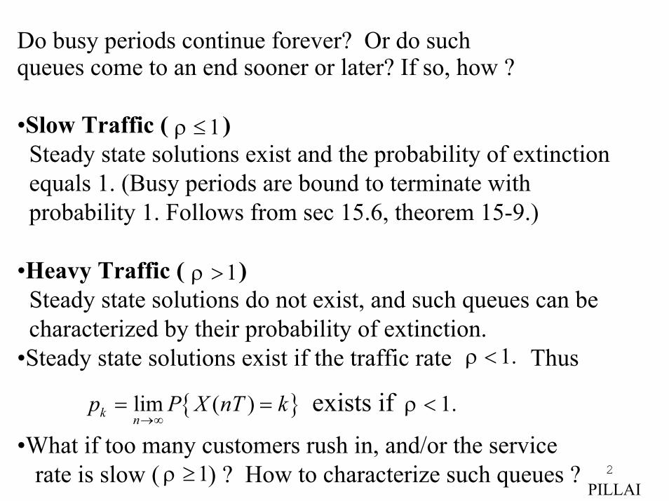
Do busy periods continue forever? Or do such queues come to an end sooner or later? If so, how ?

•Slow Traffic ( )Steady state solutions exist and the probability of extinctionequals 1. (Busy periods are bound to terminate withprobability 1. Follows from sec 15.6, theorem 15-9.)

•Heavy Traffic ( )Steady state solutions do not exist, and such queues can be characterized by their probability of extinction.

•Steady state solutions exist if the traffic rate Thus

•What if too many customers rush in, and/or the servicerate is slow ( ) ? How to characterize such queues ?

.1<ρ

{ }lim ( ) 1.exists ifk np P X nT k ρ

→∞= = <

1≥ρ

1≤ρ

1>ρ

PILLAI

3

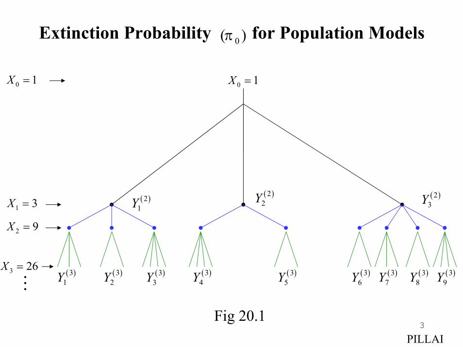
Extinction Probability for Population Models)( 0π

3 26X =

1 3X =

2 9X =

( )21Y

( )22Y ( )2

3Y

( )31Y ( )3

2Y ( )33Y ( )3

5Y( )34Y ( )3

6Y ( )38Y( )3

7Y ( )39Y

0 1X = 0 1X =

Fig 20.1PILLAI

4

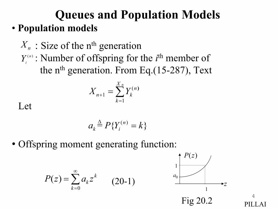
• Offspring moment generating function:

∑∞

==

0)(

k

kk zazP

Queues and Population Models• Population models

: Size of the nth generation : Number of offspring for the ith member of

the nth generation. From Eq.(15-287), Text

nX( )n

iY

(1

1

nXn

n kk

X Y+=

= ∑ )

Let

z

)(zP

0a

1

1

PILLAI

(20-1)

Fig 20.2

( )= { }nk ia P Y k=∆

5

{ }1

1 1

1 10

( ) { } { }

( { })

{[ ( )] } { ( )} { } ( ( ))

n

jin i

Xkn n

k

YXn n

jjn n

j

P z P X k z E z

E E z X j E E z X j

E P z P z P X j P P z

+

+ =

∞

+ +=

= = =

∑= = = =

= = = =

∑

∑

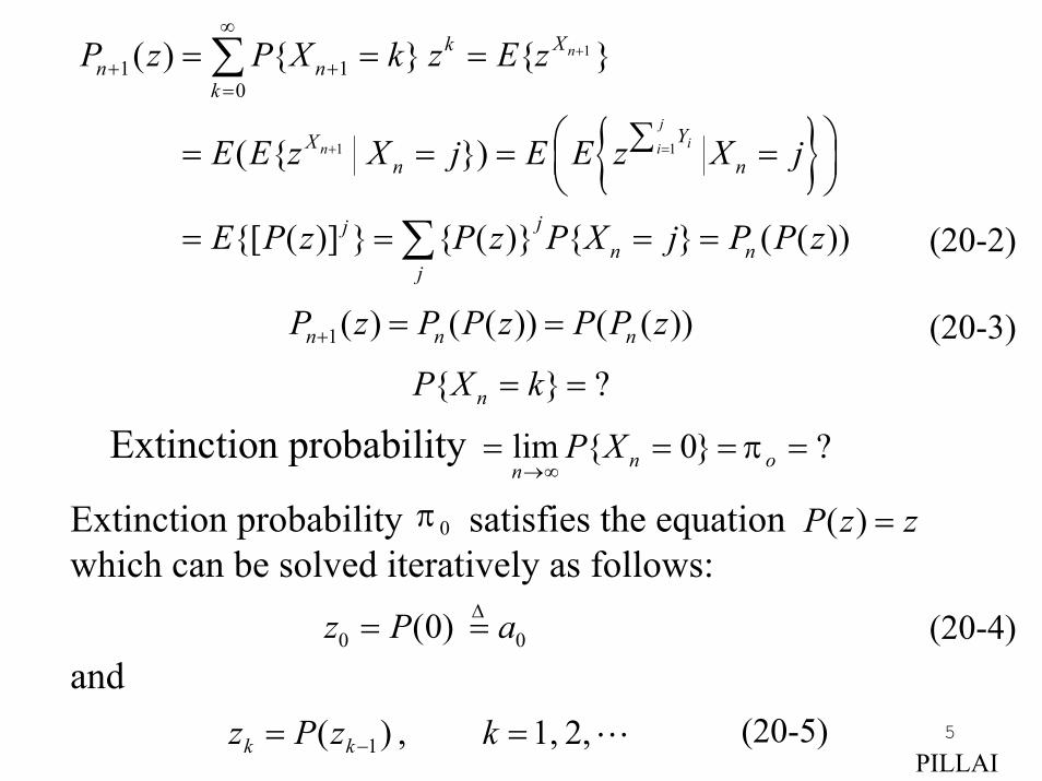
))(())(()(1 zPPzPPzP nnn ==+

Extinction probability satisfies the equation which can be solved iteratively as follows:

zzP =)(0π

2, 1, , )( 1 == − kzPz kk

{ } ?nP X k= =

lim { 0} ?Extinction probability n onP X π

→∞= = = =

and

PILLAI

(20-2)

(20-3)

(20-4)

(20-5)

0 0(0)z P a= =∆

6

Let0 0

( ) (1) { } 0i i kk k

E Y P k P Y k kaρ∞ ∞

= =

′= = = = = >∑ ∑

0

0

0 0

1 11 ( ) ,

1is the unique solution of P z z

a

ρ π

ρ ππ

≤ ⇒ = > ⇒ = < <

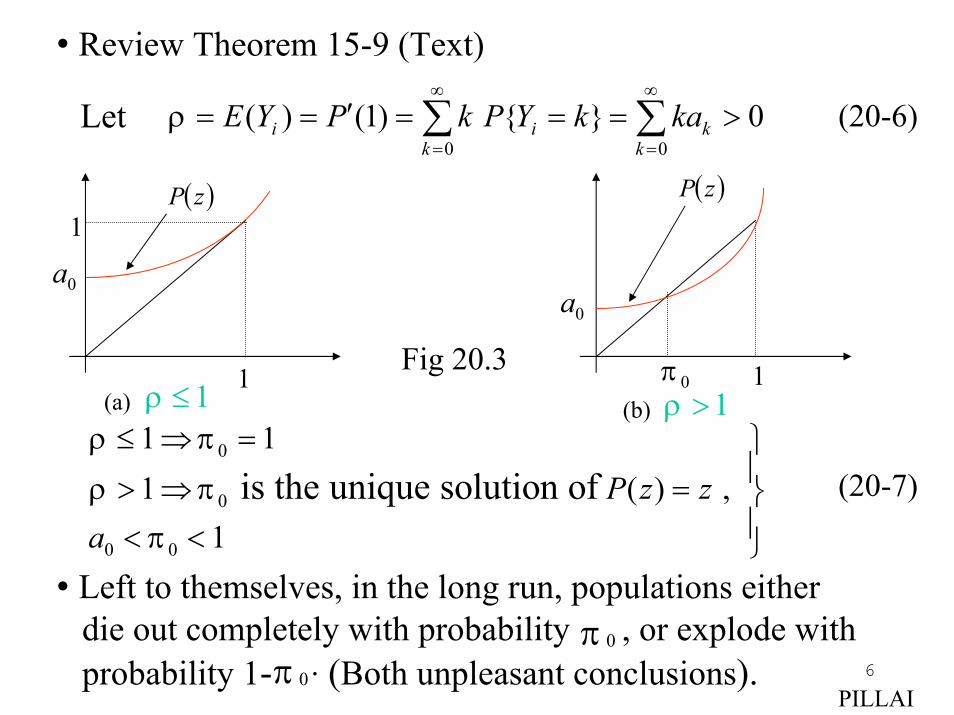
• Left to themselves, in the long run, populations either die out completely with probability , or explode with probability 1- (Both unpleasant conclusions).

π 0.0π

• Review Theorem 15-9 (Text)

PILLAI

(20-6)

(20-7)

0a

0π 11

( )zP

1≤ρ 1>ρ

0a

(a) (b)

1( )zP

Fig 20.3

7

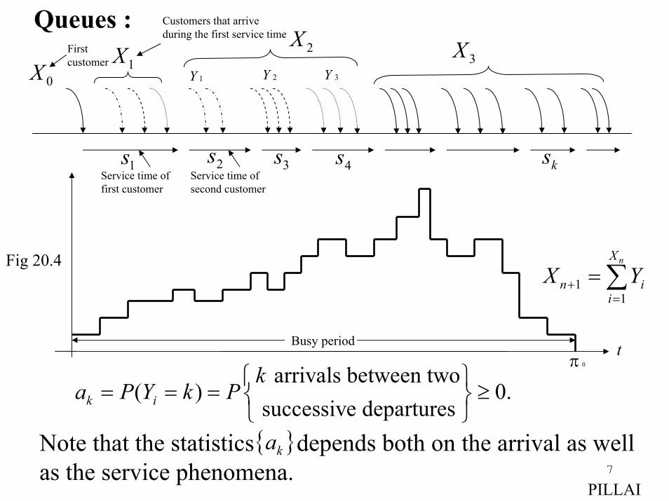
arrivals between two( ) 0.

successive departuresk i

ka P Y k P

= = = ≥

Note that the statistics depends both on the arrival as well as the service phenomena.

{ }ka

Queues :

2s

2X1Y

tπ 0

1X0X

3X

1s 3s 4s

2Y 3Y

ks

11

nX

n ii

X Y+=

= ∑

Customers that arrive during the first service time

Service time offirst customer

Service time ofsecond customer

Firstcustomer

Busy period

PILLAI

Fig 20.4

8

• : Inter-departure statistics generated by arrivals )(0∑∞

==

k

kk zazP

• : Traffic Intensity Steady stateHeavy traffic

∑∞

==′=

1)1(

kkkaPρ 1≤

• Termination of busy periods corresponds to extinction of queues. From the analogy with population models theextinction probability is the unique root of the equation0π

zzP =)(

• Slow Traffic : Heavy Traffic :i.e., unstable queues either terminate their busy periods with probability , or they will continue to be busy with probability 1- . Interestingly, there is a finite probability of busy period termination even for unstable queues.

: Measure of stability for unstable queues.

10 1 0 <<⇒> πρ1 1 0 =⇒≤ πρ

10 <π0π

0π

1> ⇒}

( 1)ρ >

PILLAI

9

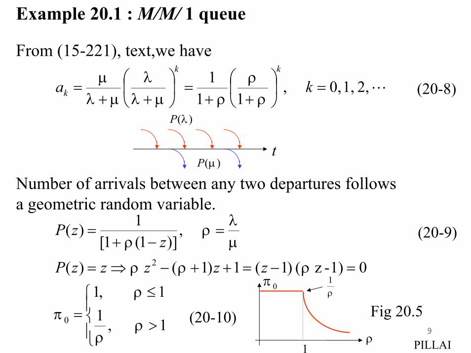
Example 20.1 : M/M/ 1 queue

2, 1, 0, ,11

1=

++

=

++

= kakk

k ρρ

ρµλλ

µλµ

0π

ρ1

ρ1

From (15-221), text,we have

t

)(λP

)(µP

Number of arrivals between any two departures follows a geometric random variable.

>

≤=

=−=++−⇒=

=−+

=

1 ,11 ,1

01)-z ( )1(1)1( )(

,)]1(1[

1)(

0

2

ρρ

ρπ

ρρρ

µλ

ρρ

zzzzzPz

zP

PILLAI

(20-8)

(20-10)

(20-9)

Fig 20.5

10

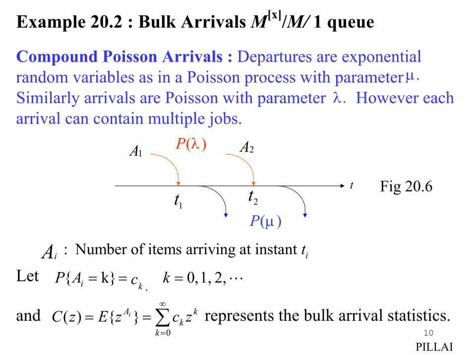
Example 20.2 : Bulk Arrivals M[x]/M/ 1 queue

Compound Poisson Arrivals : Departures are exponentialrandom variables as in a Poisson process with parameter Similarly arrivals are Poisson with parameter However eacharrival can contain multiple jobs.

2, 1, ,0 k}{,

=== kcAPki

.µ

: Number of items arriving at instant ii tA

∑∞

===

0}{)(

k

kk

A zczEzC i

Let

and represents the bulk arrival statistics.

PILLAI

.λ

A1 A2)(λP

)(µP

t

1t 2tFig 20.6

11

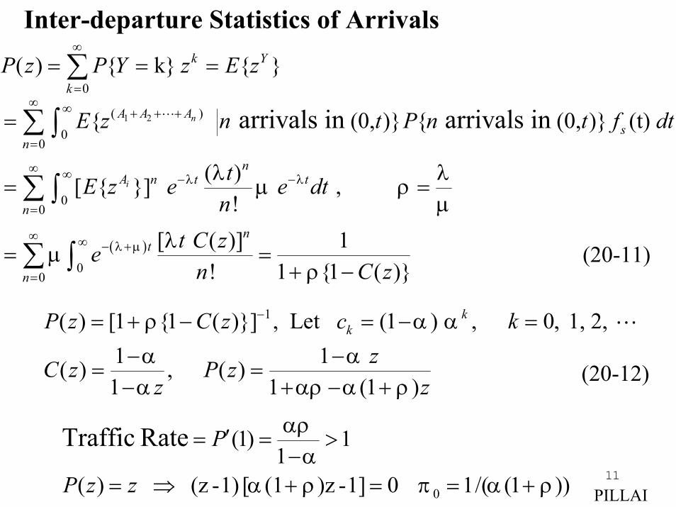
Inter-departure Statistics of Arrivals

1( ) [1 {1 ( )}] , Let (1 ) , 0, 1, 2, 1 1 ( ) , ( )1 1 (1 )

kkP z C z c k

zC z P zz z

ρ α αα αα αρ α ρ

−= + − = − =− −

= =− + − +

))1(/(1 01]-)z(1[ 1)-(z )(

11

)1(

0

Rate Traffic

ραπραα

αρ

+==+⇒=

>−

=′=

zzP

P

0( ) { k} { }k Y

kP z P Y z E z

∞

== = =∑

( )

1 2 ( ) 0

0

00

00

{ (0, )} { (0, )} (t)

( )[ { }] , !

[ ( )] 1! 1 {1 ( )}

arrivals in arrivals inn

i

A A As

nn

A n t t

n

nt

n

E z n t P n t f dt

tE z e e dtn

t C zen C z

λ λ

λ µ

λ λµ ρ

µ

λµ

ρ

∞ ∞ + + +

=

∞ ∞ − −

=

∞ ∞ − +

=

=

= =

= =+ −

∑∫

∑∫

∑ ∫

PILLAI

(20-11)

(20-12)

12

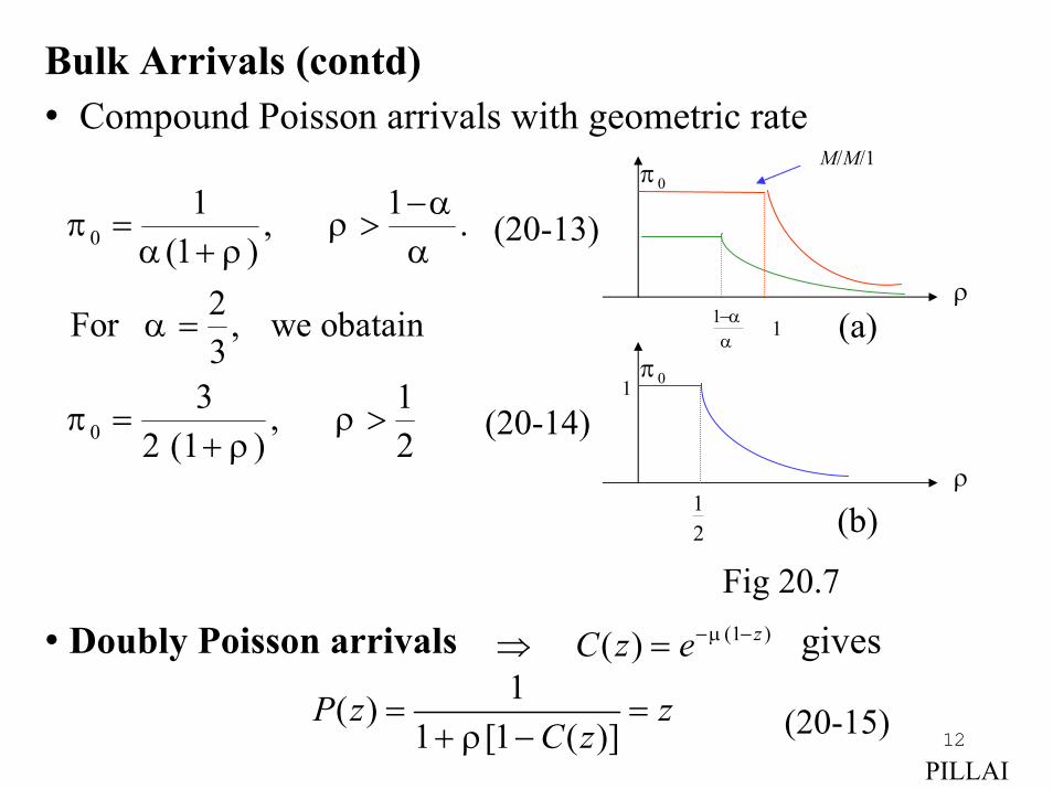
Bulk Arrivals (contd)• Compound Poisson arrivals with geometric rate

0

0

1 1, .(1 )

2For , we obatain3

3 1, 2 (1 ) 2

απ ρ

α ρ α

α

π ρρ

−= >

+

=

= >+

• Doubly Poisson arrivals gives(1 ) ( ) zC z e µ− −⇒ =

PILLAI

1( )1 [1 ( )]

P z zC zρ

= =+ −

(20-13)

(20-14)

(20-15)

0π

ρ

ρ

21

αα−1 1

0π

M/M/1

(a)

(b)

Fig 20.7

1

13

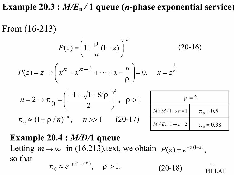
Example 20.3 : M/En / 1 queue (n-phase exponential service)

From (16-213)

11 =→ n/M/M

21 2 =→ n/E/M

5.00 =π

38.00 =π

2=ρ

Example 20.4 : M/D/1 queueLetting in (16.213),text, we obtainso that

1 , 2

81102

2

>

++−=⇒= ρ

ρπn

m →∞

.1 ,)1(0 >≈

−−− ρπρρ ee

0 (1 / ) , 1nn nπ ρ −≈ + >> (20-17)

n

zn

zP−

−+= )1(1)( ρ

nzxnxnxnxzzP1

,01)( ==

−++−+⇒=ρ

(20-16)

,)( )1( zezP −−= ρ

PILLAI(20-18)

14

20.2 Martingales

Martingales refer to a specific class of stochastic processes that maintain a form of “stability” in an overall sense. Let

refer to a discrete time stochastic process. If n refersto the present instant, then in any realization the random variables are known, and the future values

are unknown. The process is “stable” in the sense that conditioned on the available information (past and present), no change is expected on the average for the futurevalues, and hence the conditional expectation of the immediate future value is the same as that of the present value. Thus, if

{ , 0}iX i ≥

0 1, , , nX X X1 2, ,n nX X+ +

(20-19)1 1 1 0{ | , , , , }n n n nE X X X X X X+ − =

PILLAI

15

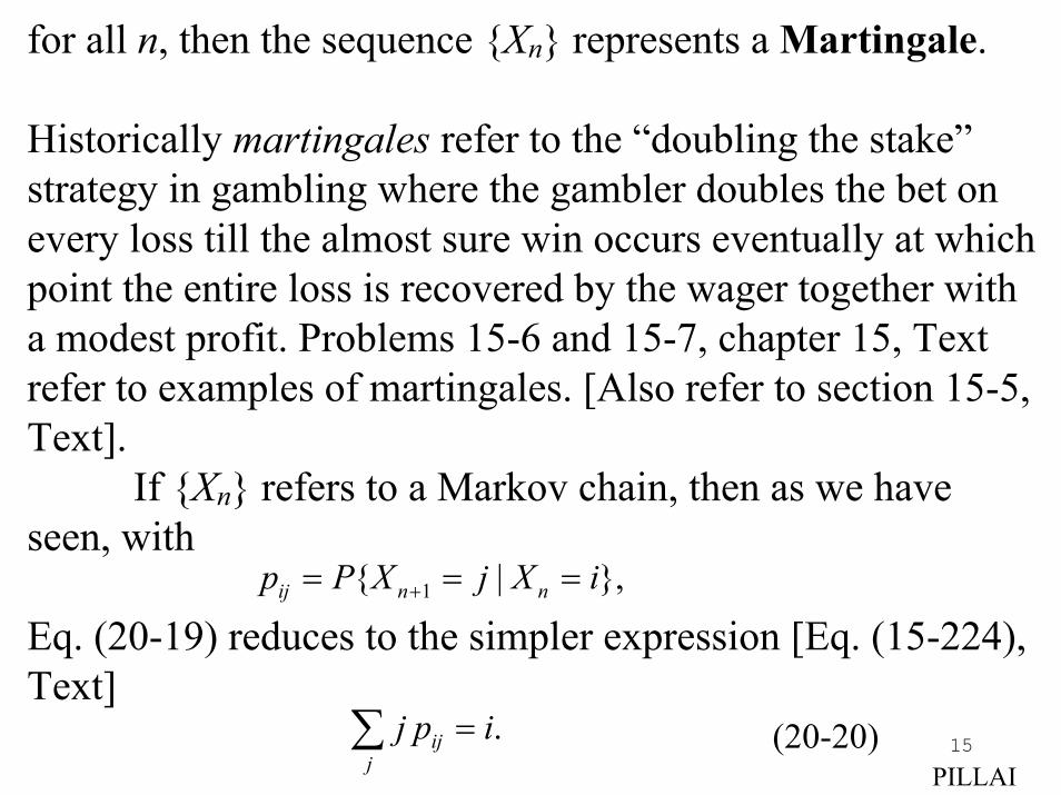
for all n, then the sequence {Xn} represents a Martingale.

Historically martingales refer to the “doubling the stake”strategy in gambling where the gambler doubles the bet on every loss till the almost sure win occurs eventually at whichpoint the entire loss is recovered by the wager together witha modest profit. Problems 15-6 and 15-7, chapter 15, Text refer to examples of martingales. [Also refer to section 15-5,Text].

If {Xn} refers to a Markov chain, then as we have seen, with

Eq. (20-19) reduces to the simpler expression [Eq. (15-224), Text]

1{ | },ij n np P X j X i+= = =

.ijj

j p i=∑ (20-20)PILLAI

16

PILLAI

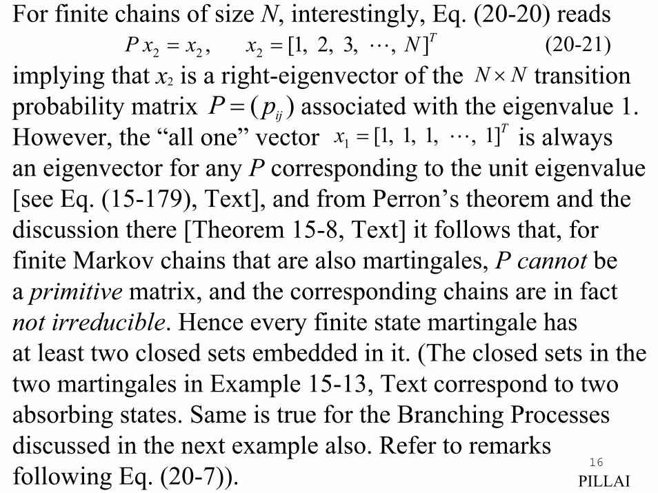
For finite chains of size N, interestingly, Eq. (20-20) reads

implying that x2 is a right-eigenvector of the transitionprobability matrix associated with the eigenvalue 1. However, the “all one” vector is alwaysan eigenvector for any P corresponding to the unit eigenvalue[see Eq. (15-179), Text], and from Perron’s theorem and the discussion there [Theorem 15-8, Text] it follows that, for finite Markov chains that are also martingales, P cannot be a primitive matrix, and the corresponding chains are in fact not irreducible. Hence every finite state martingale has at least two closed sets embedded in it. (The closed sets in thetwo martingales in Example 15-13, Text correspond to two absorbing states. Same is true for the Branching Processes discussed in the next example also. Refer to remarks following Eq. (20-7)).

2 2 2, [1, 2, 3, , ]TP x x x N= = (20-21)N N×

1 [1, 1, 1, , 1]Tx =( )ijP p=

17

PILLAI

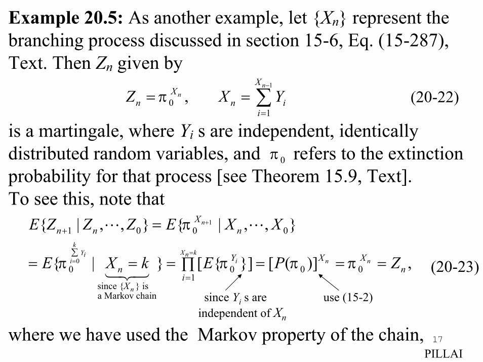
Example 20.5: As another example, let {Xn} represent the branching process discussed in section 15-6, Eq. (15-287), Text. Then Zn given by

is a martingale, where Yi s are independent, identically distributed random variables, and refers to the extinctionprobability for that process [see Theorem 15.9, Text]. To see this, note that

where we have used the Markov property of the chain,

1

01

, n

n

XX

n n ii

Z X Yπ−

== = ∑ (20-22)

0π

1

0

1 0 0 0

0 0 0 01

since { } is a Markov chain

{ | , , } { | , , }

{ | } [ { }] [ ( )] ,

n

kX kY ni

i i n n

n

Xn n n

Y X Xn n

iX

E Z Z Z E X X

E X k E P Z

π

π π π π

+

==

+

∑

=

=

= = = = = =∏ (20-23)

since Yi s are independent of Xn

use (15-2)

18

PILLAI

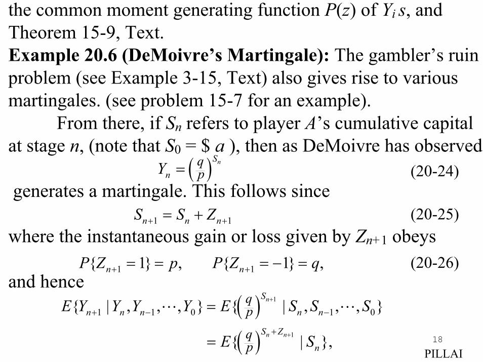
the common moment generating function P(z) of Yi s, and Theorem 15-9, Text.Example 20.6 (DeMoivre’s Martingale): The gambler’s ruinproblem (see Example 3-15, Text) also gives rise to various martingales. (see problem 15-7 for an example).

From there, if Sn refers to player A’s cumulative capitalat stage n, (note that S0 = $ a ), then as DeMoivre has observed

generates a martingale. This follows since

where the instantaneous gain or loss given by Zn+1 obeys

and hence

( ) nS

nqpY = (20-24)

1 1n n nS S Z+ += + (20-25)

1 1{ 1} , { 1} ,n nP Z p P Z q+ += = = − = (20-26)

( )( )

1

1

1 1 0 1 0{ | , , , } { | , , , }

{ | },

n

n n

S

n n n n n

S Z

n

qp

qp

E Y Y Y Y E S S S

E S

+

+

+ − −

+

=

=

19

( ) ( )( ) ( )1

1 1 0{ | , , , } n nS S

n n n nq q q qp p p pE Y Y Y Y p q Y

−

+ − ⋅= + ⋅ = =

PILLAI

since {Sn} generates a Markov chain.Thus

i.e., Yn in (20-24) defines a martingale!Martingales have excellent convergence properties

in the long run. To start with, from (20-19) for any givenn, taking expectations on both sides we get

Observe that, as stated, (20-28) is true only when n is knownor n is a given number.

As the following result shows, martingales do not fluctuate wildly. There is in fact only a small probability that a large deviation for a martingale from its initial value will occur.

(20-27)

1 0{ } { } { }.n nE X E X E X+ = = (20-28)

20

PILLAI

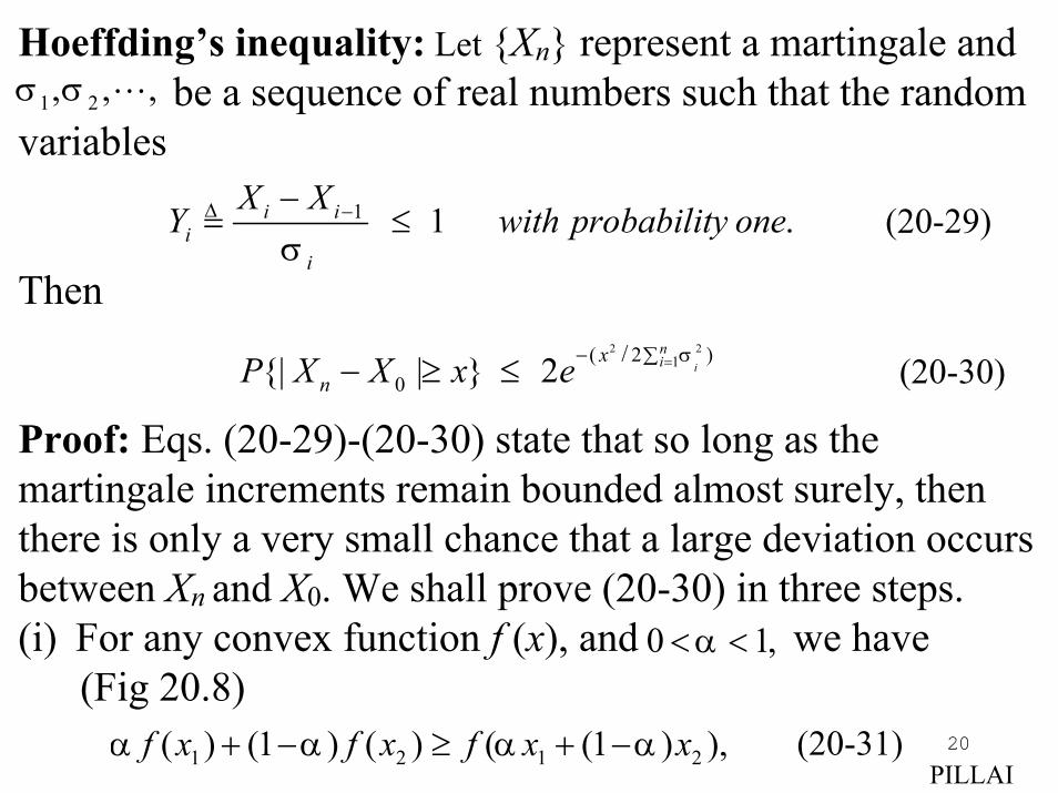
Hoeffding’s inequality: Let {Xn} represent a martingale and be a sequence of real numbers such that the random

variables

Then

Proof: Eqs. (20-29)-(20-30) state that so long as the martingale increments remain bounded almost surely, then there is only a very small chance that a large deviation occursbetween Xn and X0. We shall prove (20-30) in three steps.(i) For any convex function f (x), and we have

(Fig 20.8)

1 2, , ,σ σ

2 21( 2 )

0/{| | } 2 i

nix

nP X X x e σ=− ∑− ≥ ≤ (20-30)

(20-29)

0 1,α< <

1 2 1 2( ) (1 ) ( ) ( (1 ) ),f x f x f x xα α α α+ − ≥ + − (20-31)

1 1 .i ii

i

X XY with probability one

σ−−

= ≤∆

21

PILLAI

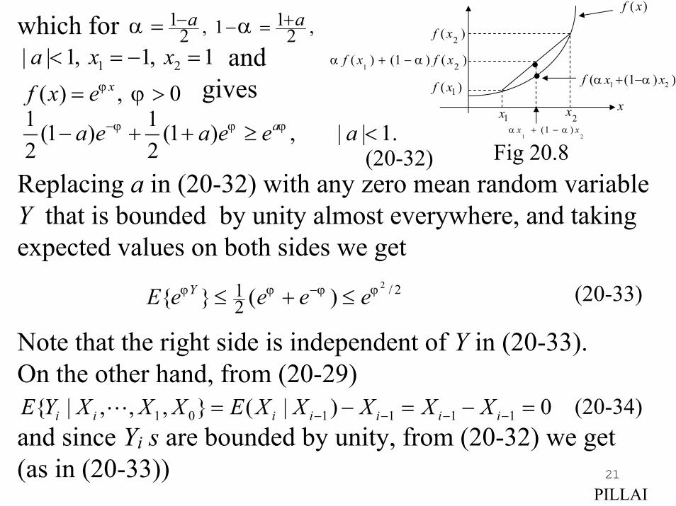
which for and

gives

Replacing a in (20-32) with any zero mean random variable Y that is bounded by unity almost everywhere, and taking expected values on both sides we get

Note that the right side is independent of Y in (20-33).On the other hand, from (20-29)

and since Yi s are bounded by unity, from (20-32) we get(as in (20-33))

1 1, 1 ,2 2a aα α− +− ==

1 2| | 1, 1, 1a x x< = − =

( ) , 0xf x eϕ ϕ= >1 1(1 ) (1 ) , | | 1.2 2

aa e a e e aϕ ϕ ϕ−− + + ≥ <(20-32)

2 / 212{ } ( )YE e e e eϕ ϕ ϕ ϕ−≤ + ≤ (20-33)

1 0 1 1 1 1{ | , , , } ( | ) 0i i i i i i iE Y X X X E X X X X X− − − −= − = − = (20-34)

Fig 20.8

1x 2x1( )f x

2( )f x

( )f x

x

1 2(1 )x xα α+ −

1 2( ) (1 ) ( )f x f xα α+ −

1 2( (1 ) )f x xα α+ −ii

22

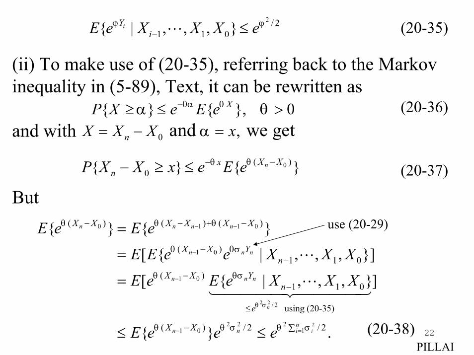
(ii) To make use of (20-35), referring back to the Markov inequality in (5-89), Text, it can be rewritten as

and with

But

2 / 21 1 0{ | , , , }iY

iE e X X X eϕ ϕ− ≤ (20-35)

{ } { }, 0XP X e E eθα θα θ−≥ ≤ >

0( )0{ } { }nX Xx

nP X X x e E eθθ −−− ≥ ≤

(20-36)

(20-37)

0 , and we getnX X X xα= − =

(20-38)PILLAI

2 2

2

0 1 1 0

1 0

1 0

/ 2

2 2 211 0

( ) ( ) ( )

( )1 1 0

( )1 1 0

using (20-35)

( ) / 2 / 2

{ } { }

[ { | , , , }]

[ { | , , , }]

{ } .

n

i

n n n n

n n n

n n n

nin n

X X X X X X

X X Yn

X X Yn

e

X X

E e E e

E E e e X X X

E e E e X X X

E e e e

θ σ

θ θ θ

θ θσ

θ θσ

θ θ σ θ σ

− −

−

−

=−

− − + −

−−

−−

≤

− ∑

=

=

=

≤ ≤

use (20-29)

23

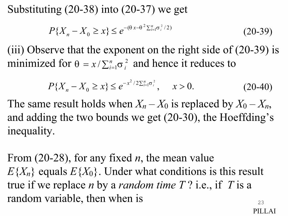
Substituting (20-38) into (20-37) we get

(iii) Observe that the exponent on the right side of (20-39) is minimized for and hence it reduces to

The same result holds when Xn – X0 is replaced by X0 – Xn, and adding the two bounds we get (20-30), the Hoeffding’s inequality.

From (20-28), for any fixed n, the mean value E{Xn} equals E{X0}. Under what conditions is this result true if we replace n by a random time T ? i.e., if T is a random variable, then when is

PILLAI

221( / 2)

0{ } inix

nP X X x e θ θ σ=− − ∑− ≥ ≤ (20-39)

21/ n

i ixθ σ== ∑

(20-40)22

1/ 20{ } , 0.i

nix

nP X X x e xσ=− ∑− ≥ ≤ >

24

The answer turns out to be that T has to be a stopping time.What is a stopping time?

A stochastic process may be known to assume a particular value, but the time at which it happens is in generalunpredictable or random. In other words, the nature of the outcome is fixed but the timing is random. When that outcomeactually occurs, the time instant corresponds to a stopping time. Consider a gambler starting with $a and let T refer to thetime instant at which his capital becomes $1. The random variable T represents a stopping time. When the capital becomes zero, it corresponds to the gambler’s ruin and that instant represents another stopping time (Time to go home for the gambler!)

PILLAI

(20-41)0{ } { }.TE X E X=?

25

Recall that in a Poisson process the occurrences of the first, second, arrivals correspond to stopping times Stopping times refer to those random instants at which thereis sufficient information to decide whether or not a specific condition is satisfied.Stopping Time: The random variable T is a stopping time for the process X(t), if for all is afunction of the values of the process up to t, i.e., it should be possible to decide whether T has occurredor not by the time t, knowing only the value of the processX(t) up to that time t. Thus the Poisson arrival times T1 and T2referred above are stopping times; however T2 – T1 is not a stopping time.

A key result in martingales states that so long as PILLAI

1 2, , .T T

0, { }the eventt T t≥ ≤

{ ( ) | 0, }X tτ τ τ> ≤

26

T is a stopping time (under some additional mild restrictions)

Notice that (20-42) generalizes (20-28) to certain random time instants (stopping times) as well.

Eq. (20-42) is an extremely useful tool in analyzing martingales. We shall illustrate its usefulness by rederiving thegambler’s ruin probability in Example 3-15, Eq. (3-47), Text.

From Example 20.6, Yn in (20-24) refer to a martingale in the gambler’s ruin problem. Let T refer to the random instant atwhich the game ends; i.e., the instant at which either player Aloses all his wealth and Pa is the associated probability of ruinfor player A, or player A gains all wealth $(a + b) with probability (1 – Pa). In that case, T is a stopping time and hence from (20-42), we get PILLAI

0{ } { }.TE X E X= (20-42)

27

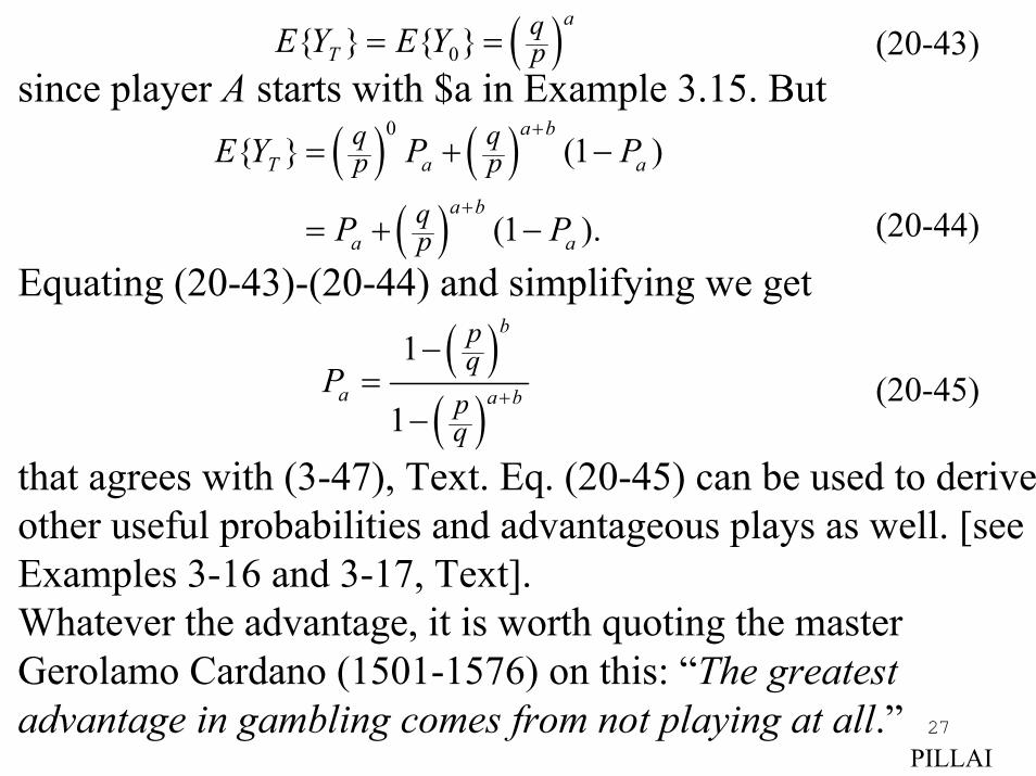
since player A starts with $a in Example 3.15. But

Equating (20-43)-(20-44) and simplifying we get

that agrees with (3-47), Text. Eq. (20-45) can be used to deriveother useful probabilities and advantageous plays as well. [see Examples 3-16 and 3-17, Text]. Whatever the advantage, it is worth quoting the master Gerolamo Cardano (1501-1576) on this: “The greatestadvantage in gambling comes from not playing at all.”

PILLAI

( )( )

1

1

b

a a b

pq

pq

P +

−=

−(20-45)

( )0{ } { }a

TqpE Y E Y= = (20-43)

( ) ( )( )

0{ } (1 )

(1 ).

a b

T a a

a b

a a

q qp p

qp

E Y P P

P P

+

+

= + −

= + − (20-44)