1tgrid tutorial guide - centre de calcul régional … this manual what’s in this manual the tgrid...
TRANSCRIPT
TGrid 5.0 Tutorial Guide
April 2008
Copyright c© 2008 by ANSYS, Inc.All Rights Reserved. No part of this document may be reproduced or otherwise used in
any form without express written permission from ANSYS, Inc.
Airpak, ANSYS, ANSYS Workbench, AUTODYN, CFX, FIDAP, FloWizard, FLUENT,GAMBIT, Icechip, Icemax, Icepak, Icepro, Icewave, MixSim, POLYFLOW, TGrid, and anyand all ANSYS, Inc. brand, product, service and feature names, logos and slogans areregistered trademarks or trademarks of ANSYS, Inc. or its subsidiaries located in theUnited States or other countries. All other brand, product, service and feature names
or trademarks are the property of their respective owners.
CATIA V5 is a registered trademark of Dassault Systemes. CHEMKIN is a registeredtrademark of Reaction Design Inc.
Portions of this program include material copyrighted by PathScale Corporation2003-2004.
ANSYS, Inc.Centerra Resource Park
10 Cavendish CourtLebanon, NH 03766
Using This Manual
What’s In This Manual
The TGrid Tutorial Guide contains a few tutorials that teach you how to use TGrid fordifferent types of problems. Each tutorial contains instructions for performing tasksrelated to the features demonstrated in the tutorial.
• Tutorial 1 is a detailed tutorial designed to introduce the beginner to TGrid. Thistutorial provides explicit instructions for all steps in the tutorial.
The remaining tutorials assume that you have read or solved Tutorial 1, and thatyou are already familiar with TGrid and its interface. In these tutorials, some stepswill not be shown explicitly.
• Tutorial 2 demonstrates the mesh generation procedure for a problem that hasmultiple regions. It also describes the procedure to generate a volume mesh usingthe automatic refinement feature of TGrid.
• Tutorial 3 demonstrates the mesh generation procedure for a hybrid mesh, startingfrom a hexahedral volume mesh and a triangular boundary mesh.
• Tutorial 4 demonstrates the mesh generation procedure for a viscous hybrid mesh,starting from a triangular boundary mesh for a sedan car body.
• Tutorial 5 explains an application from the automotive industry, thus demonstrat-ing how the hexcore mesh can significantly reduce the cell count compared with afully tetrahedral mesh.
• Tutorial 6 demonstrates the creation of a hexcore mesh upto the domain boundariesfor a sedan car.
• Tutorial 7 demonstrates the use of the boundary wrapper to repair an existinggeometry. It also describes the procedure to improve the wrapper surface quality.
• Tutorial 8 demonstrates the procedure for replacing an object in the existing meshwith another by creating a cavity and remeshing it.
Where to Find the Files Used in the Tutorials
Each of the tutorials uses an existing mesh file. You will find the appropriate mesh file(and any otherrelevant files used in the tutorial) on the TGrid documentation CD. ThePreparation step of each tutorial will tell you where to find the necessary files.
c© ANSYS, Inc. April 15, 2008 i
Using This Manual
Typographical Conventions Used In This Manual
Several typographical conventions are used in the text of the tutorials to facilitate yourlearning process.
• An informational icon ( i ) marks an important note.
• A warning icon ( ! ) marks an important note or warning.
• Different type styles are used to indicate graphical user interface menu items andtext interface menu items (e.g., Display Grid panel, display/grid command).
• The text interface type style is also used when illustrating exactly what appears onthe screen or exactly what you need to type in the text field in a panel.
• Instructions for performing each step in a tutorial will appear in standard type.Additional information about a step in a tutorial appears in italicized type.
• A mini flow chart is used to indicate the menu selections that lead you to a specificpanel. For example,
Display −→Grid...
indicates that the Grid... menu item can be selected from the Display pull-downmenu.
The words surrounded by boxes invoke menus (or submenus) and the arrows pointfrom a specific menu toward the item you should select from that menu.
ii c© ANSYS, Inc. April 15, 2008
Contents
1 Repairing a Boundary Mesh 1-1
Introduction . . . . . . . . . . . . . . . . . . . . . . . . . . . . . . . . . . . . . 1-1
Prerequisites . . . . . . . . . . . . . . . . . . . . . . . . . . . . . . . . . . . . 1-1
Preparation . . . . . . . . . . . . . . . . . . . . . . . . . . . . . . . . . . . . . 1-2
Step 1: Reading and Displaying the Boundary Mesh . . . . . . . . . . . . 1-3
Step 2: Check for Free and Unused Nodes . . . . . . . . . . . . . . . . . 1-5
Step 3: Repair the Boundary Mesh . . . . . . . . . . . . . . . . . . . . . 1-6
Step 4: Use the Rezoning Feature . . . . . . . . . . . . . . . . . . . . . . 1-9
Step 5: Improve the Boundary Mesh . . . . . . . . . . . . . . . . . . . . 1-11
Step 6: Check the Skewness Distribution of the Boundary Mesh . . . . . 1-12
Step 7: Repairing the Boundary Mesh Further . . . . . . . . . . . . . . . 1-13
Step 8: Generate a Multiple Region Volume Mesh . . . . . . . . . . . . . 1-24
Step 9: Check the Volume Mesh . . . . . . . . . . . . . . . . . . . . . . . 1-25
Step 10: Check and Save the Volume Mesh . . . . . . . . . . . . . . . . . 1-26
Summary . . . . . . . . . . . . . . . . . . . . . . . . . . . . . . . . . . . . . . 1-27
2 Tetrahedral Mesh Generation 2-1
Introduction . . . . . . . . . . . . . . . . . . . . . . . . . . . . . . . . . . . . . 2-1
Prerequisites . . . . . . . . . . . . . . . . . . . . . . . . . . . . . . . . . . . . 2-1
Preparation . . . . . . . . . . . . . . . . . . . . . . . . . . . . . . . . . . . . . 2-1
Step 1: Read and Display the Boundary Mesh . . . . . . . . . . . . . . . 2-2
Step 2: Generate the Mesh using the Skewness-Based Refinement Method 2-5
Step 3: Generate the Mesh using the Skewness-Based Refinement Method anda Size Function . . . . . . . . . . . . . . . . . . . . . . . . . . . . 2-10
c© ANSYS, Inc. April 15, 2008 i
CONTENTS
Step 4: Generate the Mesh using the Advancing Front Refinement Methodand a Size Function . . . . . . . . . . . . . . . . . . . . . . . . . 2-12
Step 5: Examine the Effect of the Maximum Cell Volume . . . . . . . . . 2-15
Step 6: Examine the Effect of the Growth Factor . . . . . . . . . . . . . 2-16
Step 7: Generate a Local Refinement in the Wake of the Car . . . . . . . 2-18
Step 8: Check and Save the Volume Mesh . . . . . . . . . . . . . . . . . 2-22
Summary . . . . . . . . . . . . . . . . . . . . . . . . . . . . . . . . . . . . . . 2-22
3 Zonal Hybrid Mesh Generation 3-1
Introduction . . . . . . . . . . . . . . . . . . . . . . . . . . . . . . . . . . . . . 3-1
Prerequisites . . . . . . . . . . . . . . . . . . . . . . . . . . . . . . . . . . . . 3-1
Preparation . . . . . . . . . . . . . . . . . . . . . . . . . . . . . . . . . . . . . 3-2
Step 1: Read and Display the Mesh . . . . . . . . . . . . . . . . . . . . . 3-3
Step 2: Merge the Free Nodes on the Tri/Quad Border . . . . . . . . . . 3-6
Step 3: Check the Skewness Distribution of the Boundary Mesh . . . . . 3-7
Step 4: Generate the Tetrahedral Mesh Using Pyramids to Transition Betweenthe Hexahedral and Tetrahedral Mesh . . . . . . . . . . . . . . . 3-8
Step 5: Extend the Mesh Using Prisms . . . . . . . . . . . . . . . . . . . 3-14
Step 6: Check and Save the Volume Mesh . . . . . . . . . . . . . . . . . 3-20
Step 7: Generate the Tetrahedral Mesh Using a Non-Conformal TransitionBetween the Hexahedral and Tetrahedral Mesh . . . . . . . . . . 3-23
Summary . . . . . . . . . . . . . . . . . . . . . . . . . . . . . . . . . . . . . . 3-27
4 Viscous Hybrid Mesh Generation 4-1
Introduction . . . . . . . . . . . . . . . . . . . . . . . . . . . . . . . . . . . . . 4-1
Prerequisites . . . . . . . . . . . . . . . . . . . . . . . . . . . . . . . . . . . . 4-1
Preparation . . . . . . . . . . . . . . . . . . . . . . . . . . . . . . . . . . . . . 4-2
Step 1: Read and Display the Boundary Mesh . . . . . . . . . . . . . . . 4-3
Step 2: Check for Free and Unused Nodes . . . . . . . . . . . . . . . . . 4-5
Step 3: Check the Quality of the Surface Mesh . . . . . . . . . . . . . . . 4-6
ii c© ANSYS, Inc. April 15, 2008
CONTENTS
Step 4: Set Parameters for Prism Layer Shrinkage and Manual TetrahedralMeshing . . . . . . . . . . . . . . . . . . . . . . . . . . . . . . . 4-7
Step 5: Set Parameters for Ignoring Prism Layers and Automatic Meshing 4-19
Summary . . . . . . . . . . . . . . . . . . . . . . . . . . . . . . . . . . . . . . 4-24
5 Hexcore Mesh Generation 5-1
Introduction . . . . . . . . . . . . . . . . . . . . . . . . . . . . . . . . . . . . . 5-1
Prerequisites . . . . . . . . . . . . . . . . . . . . . . . . . . . . . . . . . . . . 5-1
Preparation . . . . . . . . . . . . . . . . . . . . . . . . . . . . . . . . . . . . . 5-2
Step 1: Read and Display the Mesh . . . . . . . . . . . . . . . . . . . . . 5-3
Step 2: Check and Improve the Skewness of the Surface Mesh . . . . . . 5-5
Step 3: Repair the Boundary Mesh . . . . . . . . . . . . . . . . . . . . . 5-6
Step 4: Generate the Tetrahedral Mesh . . . . . . . . . . . . . . . . . . . 5-8
Step 5: Generate the Hexcore Mesh . . . . . . . . . . . . . . . . . . . . . 5-11
Step 6: Examine the Effect of the Buffer Layers on the Hexcore Mesh . . 5-13
Step 7: Automatically Generate the Hexcore Mesh with Prism Layers and aLocal Refinement Region . . . . . . . . . . . . . . . . . . . . . . 5-16
Summary . . . . . . . . . . . . . . . . . . . . . . . . . . . . . . . . . . . . . . 5-22
6 Generating the Hexcore Mesh Upto Domain Boundaries 6-1
Introduction . . . . . . . . . . . . . . . . . . . . . . . . . . . . . . . . . . . . . 6-1
Prerequisites . . . . . . . . . . . . . . . . . . . . . . . . . . . . . . . . . . . . 6-1
Preparation . . . . . . . . . . . . . . . . . . . . . . . . . . . . . . . . . . . . . 6-1
Step 1: Read and Display the Boundary Mesh . . . . . . . . . . . . . . . 6-2
Step 2: Delete the Outer Box Boundaries . . . . . . . . . . . . . . . . . . 6-4
Step 3: Set the Hexcore Meshing Parameters . . . . . . . . . . . . . . . . 6-5
Step 4: Automatically Generate the Hexcore Mesh Upto the Boundaries withPrism Layers . . . . . . . . . . . . . . . . . . . . . . . . . . . . . 6-7
Summary . . . . . . . . . . . . . . . . . . . . . . . . . . . . . . . . . . . . . . 6-15
c© ANSYS, Inc. April 15, 2008 iii
CONTENTS
7 Using the Boundary Wrapper 7-1
Introduction . . . . . . . . . . . . . . . . . . . . . . . . . . . . . . . . . . . . . 7-1
Prerequisites . . . . . . . . . . . . . . . . . . . . . . . . . . . . . . . . . . . . 7-1
Preparation . . . . . . . . . . . . . . . . . . . . . . . . . . . . . . . . . . . . . 7-2
Step 1: Read and Display the Mesh . . . . . . . . . . . . . . . . . . . . . 7-3
Step 2: Perform Pre-Wrapping Operations to Close Holes in the Geometry 7-4
Step 3: Initialize the Surface Wrapper . . . . . . . . . . . . . . . . . . . . 7-12
Step 4: Check the Region to be Wrapped . . . . . . . . . . . . . . . . . . 7-13
Step 5: Refine the Main Region . . . . . . . . . . . . . . . . . . . . . . . 7-18
Step 6: Close Small Holes Automatically . . . . . . . . . . . . . . . . . . 7-19
Step 7: Wrap the Main Region . . . . . . . . . . . . . . . . . . . . . . . . 7-23
Step 8: Capture Features . . . . . . . . . . . . . . . . . . . . . . . . . . . 7-24
Step 9: Post Wrapping Operations . . . . . . . . . . . . . . . . . . . . . 7-28
Step 11: Create the Tunnel . . . . . . . . . . . . . . . . . . . . . . . . . 7-38
Step 12: Generate the Volume Mesh . . . . . . . . . . . . . . . . . . . . 7-39
Step 13: Improve the Volume Mesh . . . . . . . . . . . . . . . . . . . . . 7-41
Step 14: Separate the Tunnel Inlet and Outlet . . . . . . . . . . . . . . . 7-42
Summary . . . . . . . . . . . . . . . . . . . . . . . . . . . . . . . . . . . . . . 7-43
8 Cavity Remeshing 8-1
Introduction . . . . . . . . . . . . . . . . . . . . . . . . . . . . . . . . . . . . . 8-1
Prerequisites . . . . . . . . . . . . . . . . . . . . . . . . . . . . . . . . . . . . 8-1
Preparation . . . . . . . . . . . . . . . . . . . . . . . . . . . . . . . . . . . . . 8-1
Case A. For a Tetrahedral Mesh . . . . . . . . . . . . . . . . . . . . . . . 8-2
Case B. For a Hybrid Mesh (Tetrahedra and Prisms) Having a Single FluidZone . . . . . . . . . . . . . . . . . . . . . . . . . . . . . . . . . 8-11
Case C. For a Hybrid Mesh (Tetrahedra and Prisms) Having Multiple FluidZones . . . . . . . . . . . . . . . . . . . . . . . . . . . . . . . . . 8-21
Case D. For a Hexcore Mesh . . . . . . . . . . . . . . . . . . . . . . . . . 8-24
Summary . . . . . . . . . . . . . . . . . . . . . . . . . . . . . . . . . . . . . . 8-29
iv c© ANSYS, Inc. April 15, 2008
Tutorial 1. Repairing a Boundary Mesh
Introduction
TGrid offers several tools for mesh repair. While there is no right or wrong way to repaira mesh, the goal is to improve the quality of the mesh with each mesh repair operation.This tutorial demonstrates the use of some mesh repair tools in TGrid to find and fixknown deficiencies in an existing boundary mesh (a simple 3D geometry).
This tutorial demonstrates how to do the following:
1. Read the mesh file and display the boundary mesh.
2. Check for free and unused nodes.
3. Repair the boundary mesh by recreating missing faces.
4. Use the rezoning feature.
5. Improve the boundary mesh.
6. Check the skewness of the boundary faces.
7. Further repair the boundary mesh.
8. Generate a multiple region volume mesh.
9. Check the quality of the entire volume mesh.
10. Check and save the volume mesh.
Prerequisites
This tutorial assumes that you have little experience with TGrid, but are familiar withthe graphical user interface.
c© ANSYS, Inc. April 15, 2008 1-1
Repairing a Boundary Mesh
Preparation
1. Download mesh-repair.zip from the FLUENT User Services Center to yourworking directory. This file can be found from the Documentation link on theTGrid product page.
OR
Copy mesh-repair.zip from the TGrid documentation CD to your working direc-tory.
• For UNIX systems, insert the CD into your CD-ROM drive and go to thefollowing directory:
cdrom/tgrid5.0/help/tutfiles/
where cdrom must be replaced by the name of your CD-ROM drive.
• For Windows systems, insert the CD into your CD-ROM drive and go to thefollowing folder:
cdrom:\tgrid5.0\help\tutfiles\
where, cdrom must be replaced by the name of your CD-ROM drive (e.g., E).
2. Unzip mesh-repair.zip.
The file, problem-surf.msh can be found in the mesh-repair folder created onunzipping the file.
3. Start the 3D (3d) version of TGrid.
1-2 c© ANSYS, Inc. April 15, 2008
Repairing a Boundary Mesh
Step 1: Reading and Displaying the Boundary Mesh
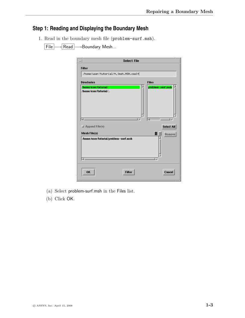
1. Read in the boundary mesh file (problem-surf.msh).
File −→ Read −→Boundary Mesh...
(a) Select problem-surf.msh in the Files list.
(b) Click OK.
c© ANSYS, Inc. April 15, 2008 1-3
Repairing a Boundary Mesh
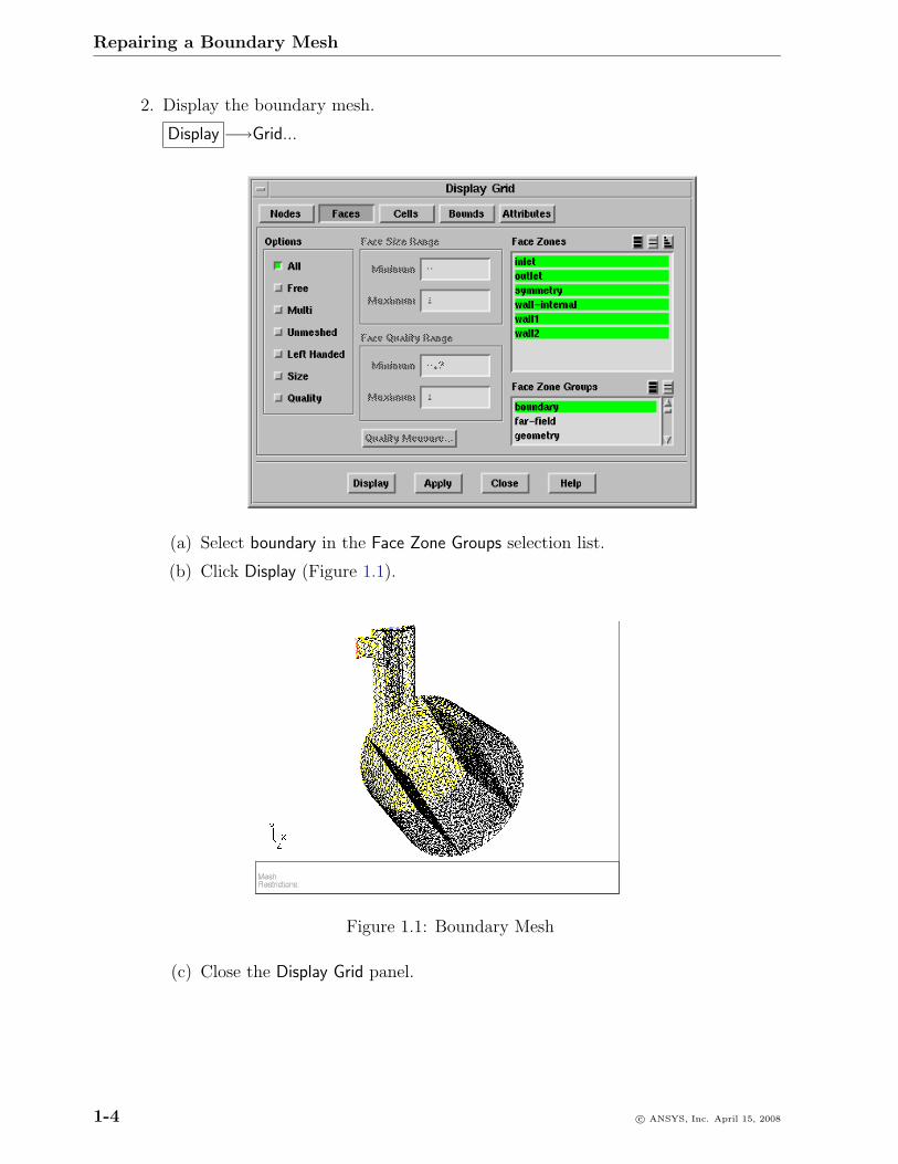
2. Display the boundary mesh.
Display −→Grid...
(a) Select boundary in the Face Zone Groups selection list.
(b) Click Display (Figure 1.1).
Figure 1.1: Boundary Mesh
(c) Close the Display Grid panel.
1-4 c© ANSYS, Inc. April 15, 2008
Repairing a Boundary Mesh
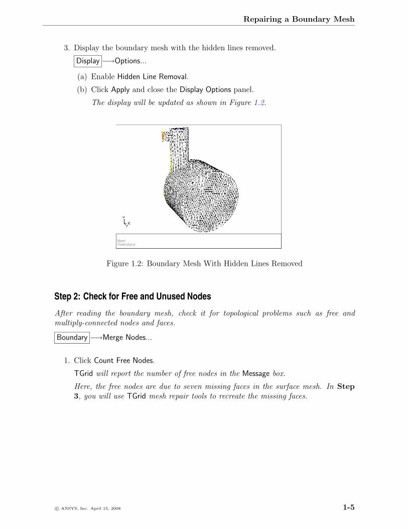
3. Display the boundary mesh with the hidden lines removed.
Display −→Options...
(a) Enable Hidden Line Removal.
(b) Click Apply and close the Display Options panel.
The display will be updated as shown in Figure 1.2.
Figure 1.2: Boundary Mesh With Hidden Lines Removed
Step 2: Check for Free and Unused Nodes
After reading the boundary mesh, check it for topological problems such as free andmultiply-connected nodes and faces.
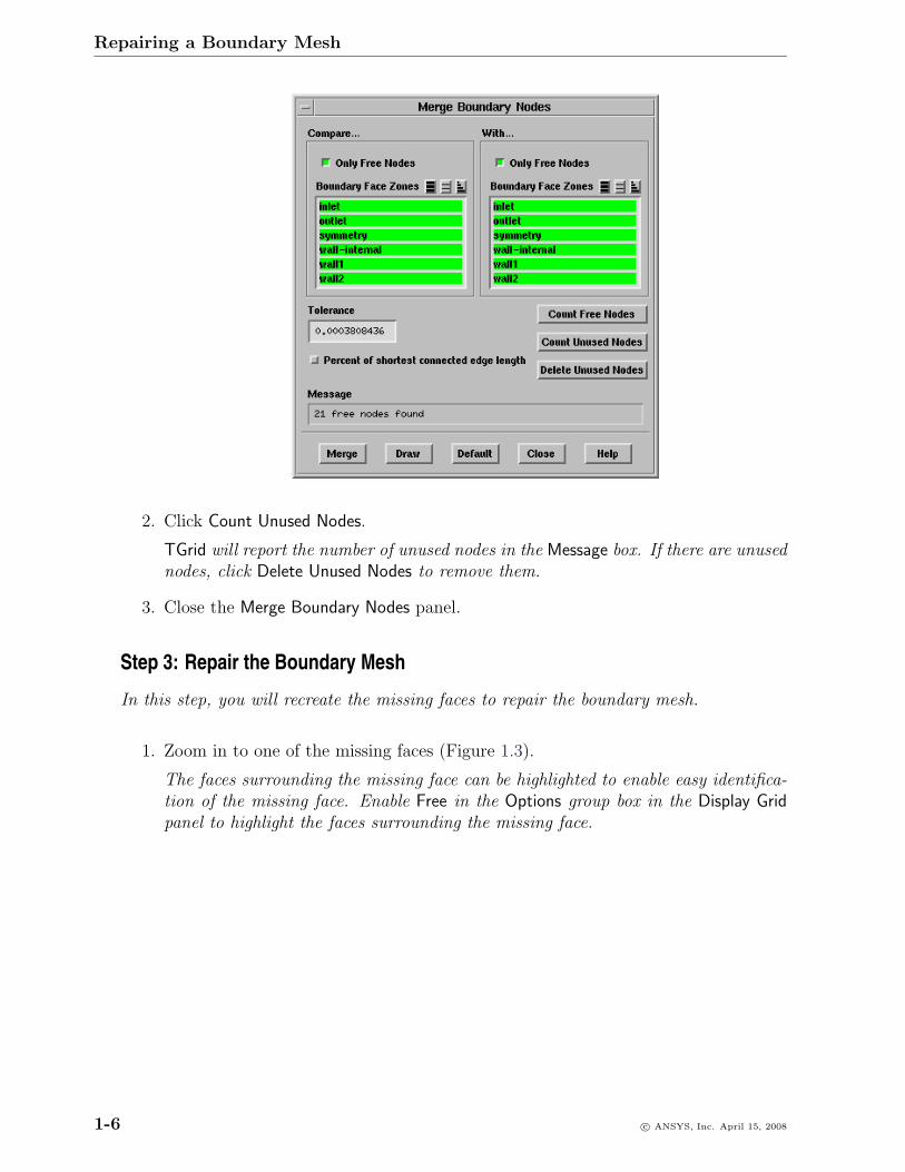
Boundary −→Merge Nodes...
1. Click Count Free Nodes.
TGrid will report the number of free nodes in the Message box.
Here, the free nodes are due to seven missing faces in the surface mesh. In Step3, you will use TGrid mesh repair tools to recreate the missing faces.
c© ANSYS, Inc. April 15, 2008 1-5
Repairing a Boundary Mesh
2. Click Count Unused Nodes.
TGrid will report the number of unused nodes in the Message box. If there are unusednodes, click Delete Unused Nodes to remove them.
3. Close the Merge Boundary Nodes panel.
Step 3: Repair the Boundary Mesh
In this step, you will recreate the missing faces to repair the boundary mesh.
1. Zoom in to one of the missing faces (Figure 1.3).
The faces surrounding the missing face can be highlighted to enable easy identifica-tion of the missing face. Enable Free in the Options group box in the Display Gridpanel to highlight the faces surrounding the missing face.
1-6 c© ANSYS, Inc. April 15, 2008
Repairing a Boundary Mesh
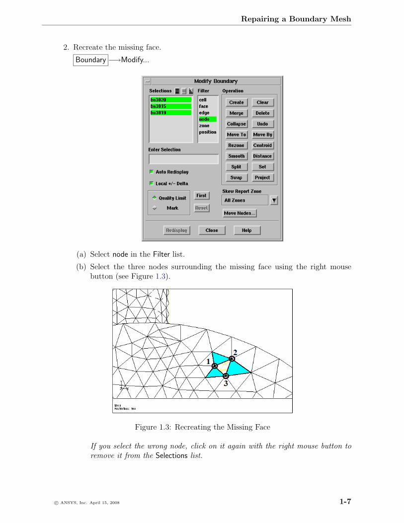
2. Recreate the missing face.
Boundary −→Modify...
(a) Select node in the Filter list.
(b) Select the three nodes surrounding the missing face using the right mousebutton (see Figure 1.3).
Figure 1.3: Recreating the Missing Face
If you select the wrong node, click on it again with the right mouse button toremove it from the Selections list.
c© ANSYS, Inc. April 15, 2008 1-7
Repairing a Boundary Mesh
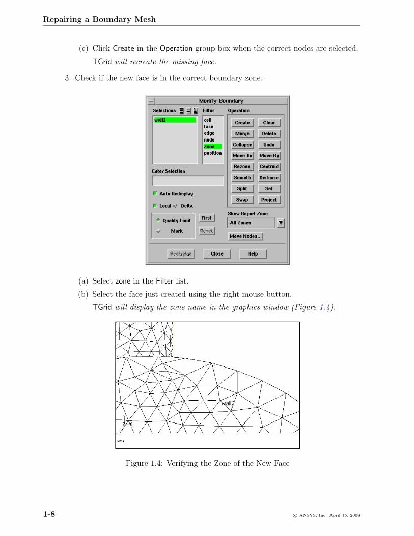
(c) Click Create in the Operation group box when the correct nodes are selected.
TGrid will recreate the missing face.
3. Check if the new face is in the correct boundary zone.
(a) Select zone in the Filter list.
(b) Select the face just created using the right mouse button.
TGrid will display the zone name in the graphics window (Figure 1.4).
Figure 1.4: Verifying the Zone of the New Face
1-8 c© ANSYS, Inc. April 15, 2008
Repairing a Boundary Mesh
TGrid places the face in the same zone as the majority of the nodes that com-prise the face. If two out of the three selected nodes are in the symmetry zone,then the face created is placed in the symmetry zone. In this example, the threenodes selected are in the wall2 zone, hence the face created is also placed in thewall2 zone.
(c) If the face is in the wrong zone, use the Rezone option in the Operation groupbox to move the face to the appropriate zone (see Step 4).
4. Similarly, recreate the other missing faces.
5. Save an intermediate mesh file (temp.msh).
File −→ Write −→Mesh...
! It is not always possible to undo an operation. Hence, it is recommendedthat you save the mesh periodically when modifying the boundary mesh.
Step 4: Use the Rezoning Feature
This step illustrates the use of the Rezone option to move a face from one zone to another.First, you will move the face from the wall2 boundary to the symmetry boundary. Whenthis step is complete, you will move the selected face back to the wall2 zone.
Boundary −→Modify...
1. Select face in the Filter list.
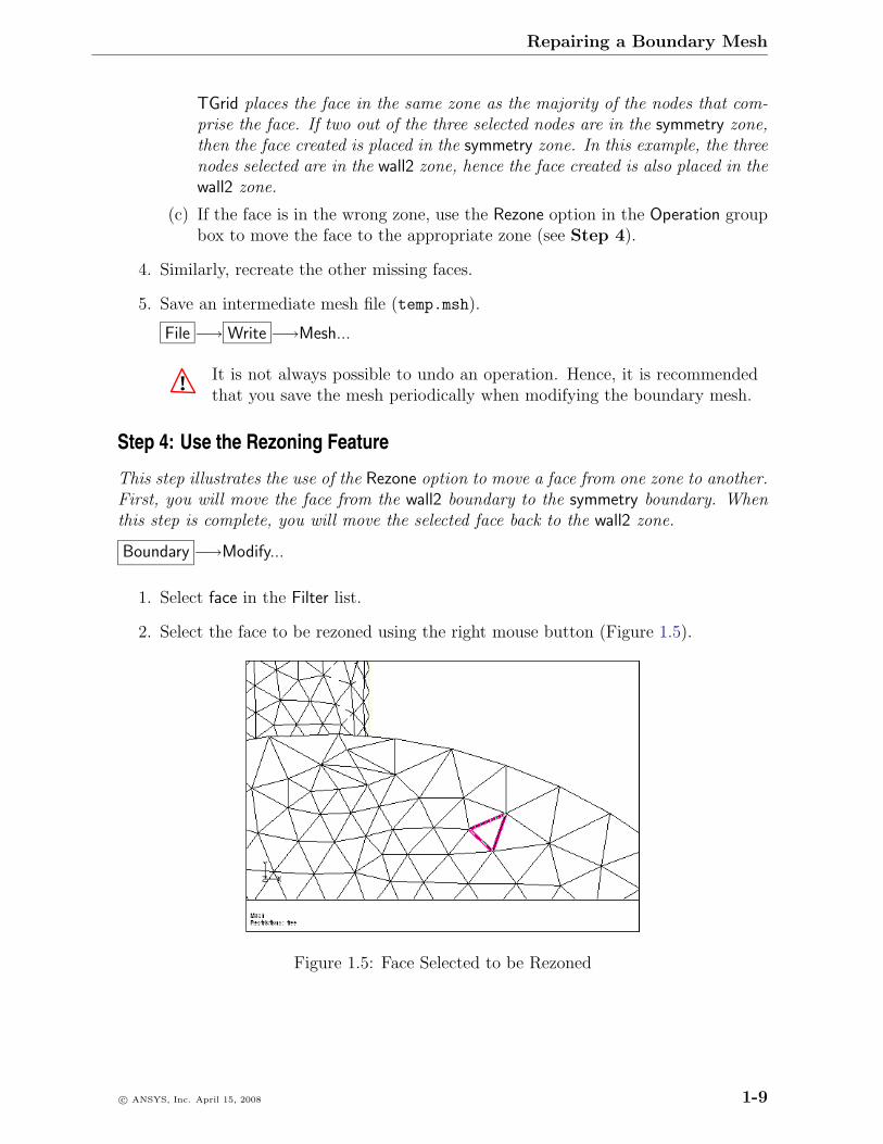
2. Select the face to be rezoned using the right mouse button (Figure 1.5).
Figure 1.5: Face Selected to be Rezoned
c© ANSYS, Inc. April 15, 2008 1-9
Repairing a Boundary Mesh
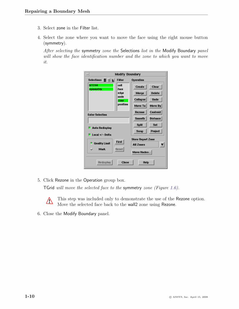
3. Select zone in the Filter list.
4. Select the zone where you want to move the face using the right mouse button(symmetry).
After selecting the symmetry zone the Selections list in the Modify Boundary panelwill show the face identification number and the zone to which you want to moveit.
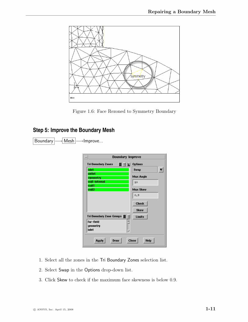
5. Click Rezone in the Operation group box.
TGrid will move the selected face to the symmetry zone (Figure 1.6).
! This step was included only to demonstrate the use of the Rezone option.Move the selected face back to the wall2 zone using Rezone.
6. Close the Modify Boundary panel.
1-10 c© ANSYS, Inc. April 15, 2008
Repairing a Boundary Mesh
Figure 1.6: Face Rezoned to Symmetry Boundary
Step 5: Improve the Boundary Mesh
Boundary −→ Mesh −→Improve...
1. Select all the zones in the Tri Boundary Zones selection list.
2. Select Swap in the Options drop-down list.
3. Click Skew to check if the maximum face skewness is below 0.9.
c© ANSYS, Inc. April 15, 2008 1-11
Repairing a Boundary Mesh
TGrid will report that the maximum face skewness is approximately 0.992.
4. Click Check to check for Delaunay violations in the boundary mesh.
TGrid will report the violations in the console.
5. Retain the default values of 10 and 0.9 for Max Angle and Max Skew, respectively.
6. Click Apply until TGrid reports zero modifications made.
7. Click Skew to verify that the maximum face skewness is below 0.9.
8. Close the Boundary Improve panel.
Step 6: Check the Skewness Distribution of the Boundary Mesh
Display −→ Plot −→Face Distribution...
1. Select all the zones in the Boundary Zones selection list.
2. Enter 10 for Partitions.
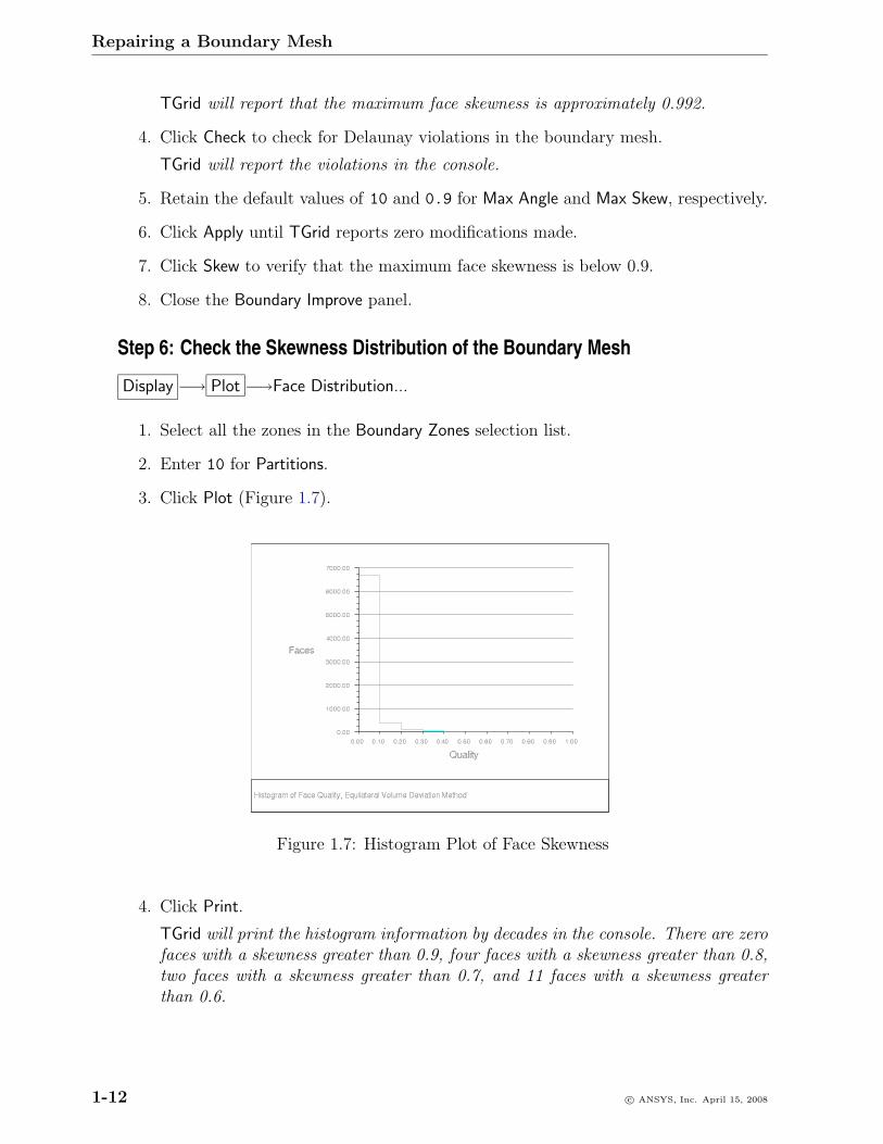
3. Click Plot (Figure 1.7).
Figure 1.7: Histogram Plot of Face Skewness
4. Click Print.
TGrid will print the histogram information by decades in the console. There are zerofaces with a skewness greater than 0.9, four faces with a skewness greater than 0.8,two faces with a skewness greater than 0.7, and 11 faces with a skewness greaterthan 0.6.
1-12 c© ANSYS, Inc. April 15, 2008
Repairing a Boundary Mesh
5. Close the Face Distribution panel.
Extra: This tutorial also aims at reducing the maximum face skewness below 0.6. Thistutorial exposes you to some of the mesh repair tools. Then, it is up to you to tryand get the maximum face skewness below 0.6.
Step 7: Repairing the Boundary Mesh Further
In this step, you will repair the mesh by merging and smoothing nodes, swapping andsplitting edges, and splitting faces.
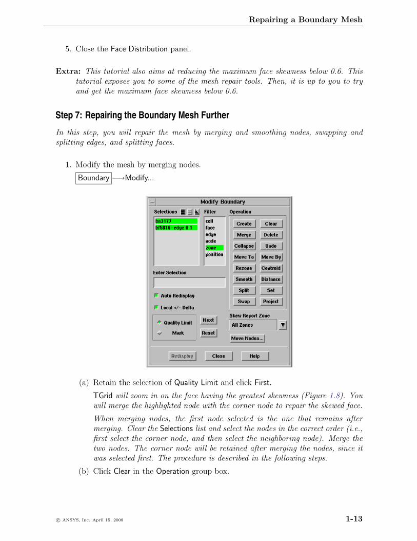
1. Modify the mesh by merging nodes.
Boundary −→Modify...
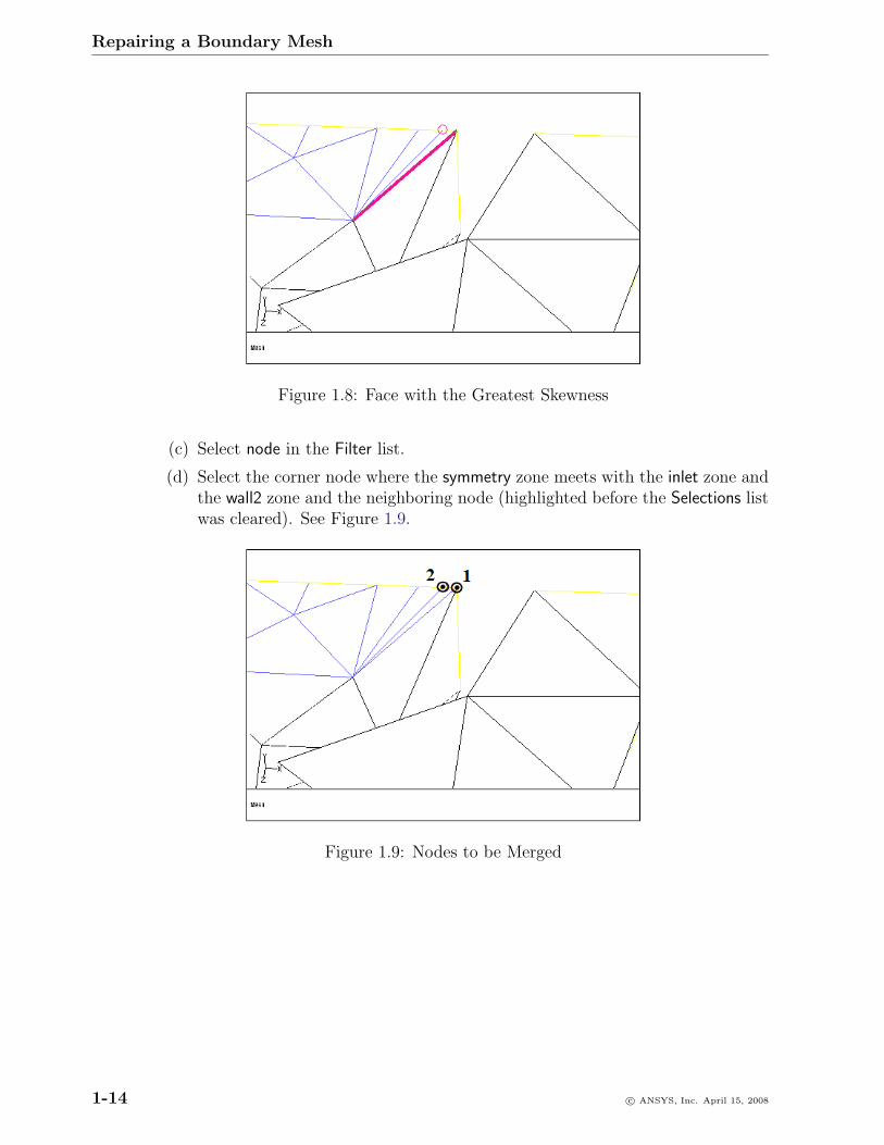
(a) Retain the selection of Quality Limit and click First.
TGrid will zoom in on the face having the greatest skewness (Figure 1.8). Youwill merge the highlighted node with the corner node to repair the skewed face.
When merging nodes, the first node selected is the one that remains aftermerging. Clear the Selections list and select the nodes in the correct order (i.e.,first select the corner node, and then select the neighboring node). Merge thetwo nodes. The corner node will be retained after merging the nodes, since itwas selected first. The procedure is described in the following steps.
(b) Click Clear in the Operation group box.
c© ANSYS, Inc. April 15, 2008 1-13
Repairing a Boundary Mesh
Figure 1.8: Face with the Greatest Skewness
(c) Select node in the Filter list.
(d) Select the corner node where the symmetry zone meets with the inlet zone andthe wall2 zone and the neighboring node (highlighted before the Selections listwas cleared). See Figure 1.9.
Figure 1.9: Nodes to be Merged
1-14 c© ANSYS, Inc. April 15, 2008
Repairing a Boundary Mesh
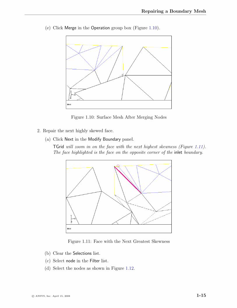
(e) Click Merge in the Operation group box (Figure 1.10).
Figure 1.10: Surface Mesh After Merging Nodes
2. Repair the next highly skewed face.
(a) Click Next in the Modify Boundary panel.
TGrid will zoom in on the face with the next highest skewness (Figure 1.11).The face highlighted is the face on the opposite corner of the inlet boundary.
Figure 1.11: Face with the Next Greatest Skewness
(b) Clear the Selections list.
(c) Select node in the Filter list.
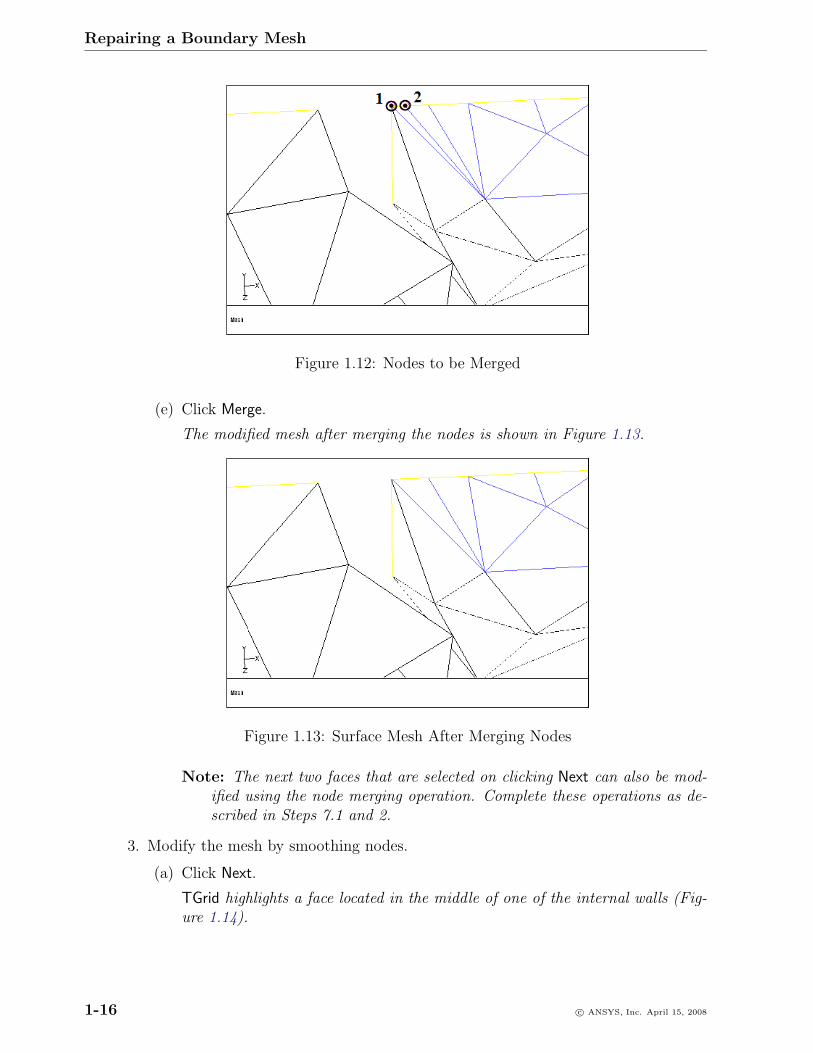
(d) Select the nodes as shown in Figure 1.12.
c© ANSYS, Inc. April 15, 2008 1-15
Repairing a Boundary Mesh
Figure 1.12: Nodes to be Merged
(e) Click Merge.
The modified mesh after merging the nodes is shown in Figure 1.13.
Figure 1.13: Surface Mesh After Merging Nodes
Note: The next two faces that are selected on clicking Next can also be mod-ified using the node merging operation. Complete these operations as de-scribed in Steps 7.1 and 2.
3. Modify the mesh by smoothing nodes.
(a) Click Next.
TGrid highlights a face located in the middle of one of the internal walls (Fig-ure 1.14).
1-16 c© ANSYS, Inc. April 15, 2008
Repairing a Boundary Mesh
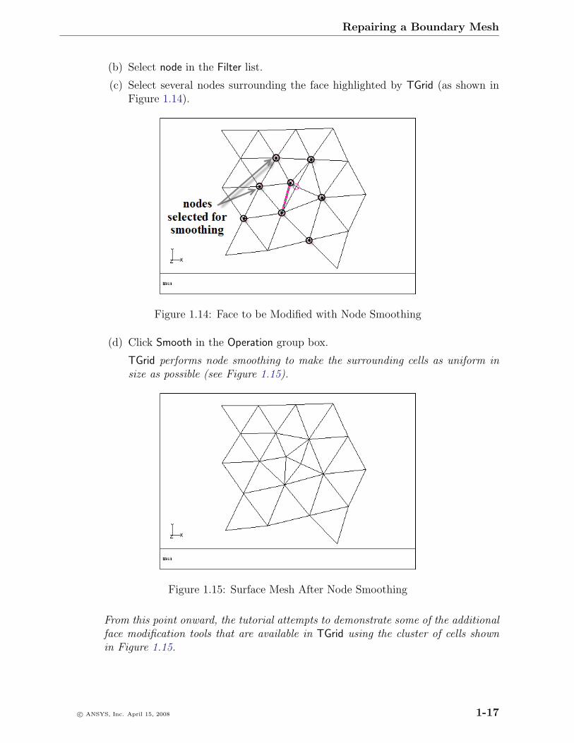
(b) Select node in the Filter list.
(c) Select several nodes surrounding the face highlighted by TGrid (as shown inFigure 1.14).
Figure 1.14: Face to be Modified with Node Smoothing
(d) Click Smooth in the Operation group box.
TGrid performs node smoothing to make the surrounding cells as uniform insize as possible (see Figure 1.15).
Figure 1.15: Surface Mesh After Node Smoothing
From this point onward, the tutorial attempts to demonstrate some of the additionalface modification tools that are available in TGrid using the cluster of cells shownin Figure 1.15.
c© ANSYS, Inc. April 15, 2008 1-17
Repairing a Boundary Mesh
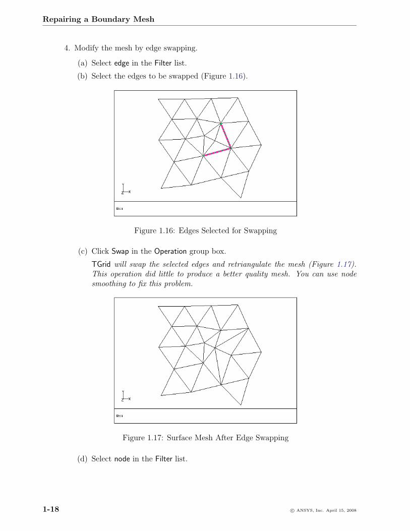
4. Modify the mesh by edge swapping.
(a) Select edge in the Filter list.
(b) Select the edges to be swapped (Figure 1.16).
Figure 1.16: Edges Selected for Swapping
(c) Click Swap in the Operation group box.
TGrid will swap the selected edges and retriangulate the mesh (Figure 1.17).This operation did little to produce a better quality mesh. You can use nodesmoothing to fix this problem.
Figure 1.17: Surface Mesh After Edge Swapping
(d) Select node in the Filter list.
1-18 c© ANSYS, Inc. April 15, 2008
Repairing a Boundary Mesh
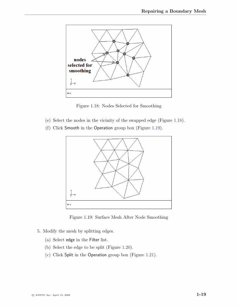
Figure 1.18: Nodes Selected for Smoothing
(e) Select the nodes in the vicinity of the swapped edge (Figure 1.18).
(f) Click Smooth in the Operation group box (Figure 1.19).
Figure 1.19: Surface Mesh After Node Smoothing
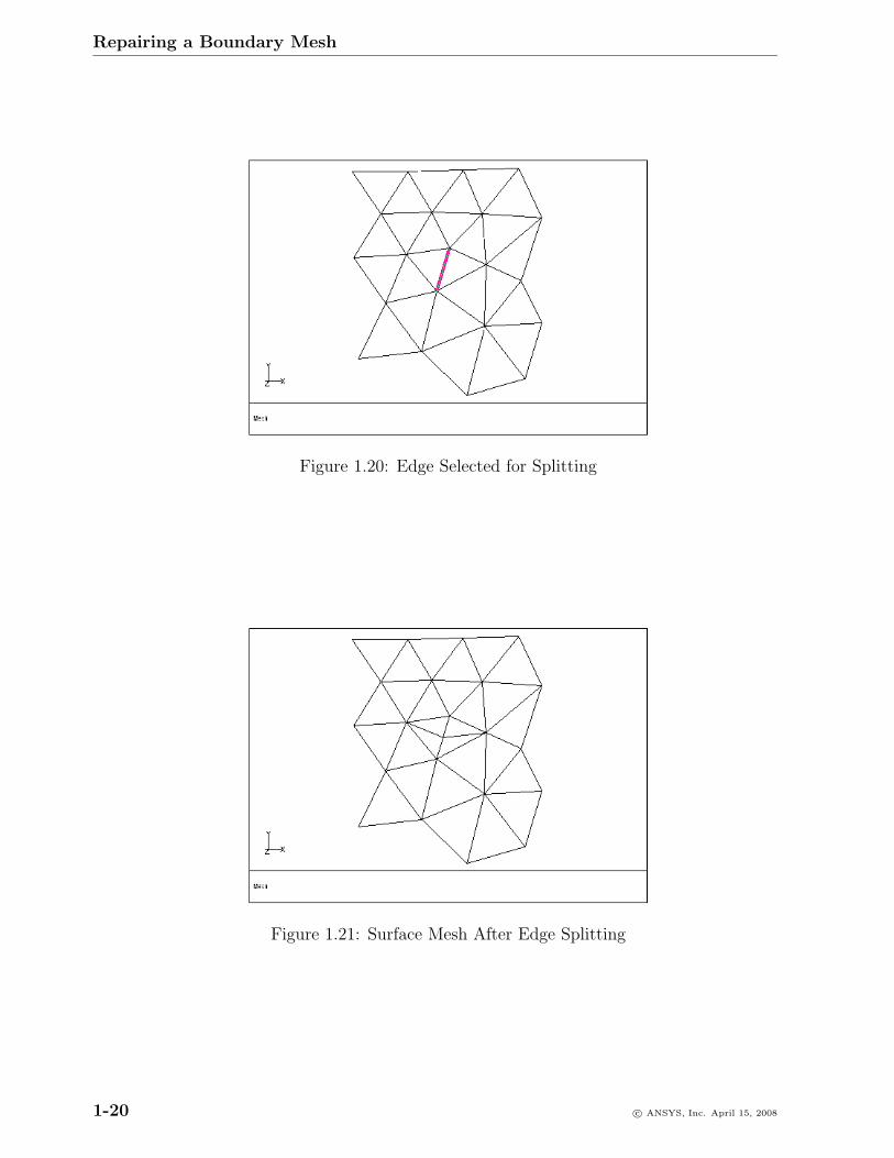
5. Modify the mesh by splitting edges.
(a) Select edge in the Filter list.
(b) Select the edge to be split (Figure 1.20).
(c) Click Split in the Operation group box (Figure 1.21).
c© ANSYS, Inc. April 15, 2008 1-19
Repairing a Boundary Mesh
Figure 1.20: Edge Selected for Splitting
Figure 1.21: Surface Mesh After Edge Splitting
1-20 c© ANSYS, Inc. April 15, 2008
Repairing a Boundary Mesh
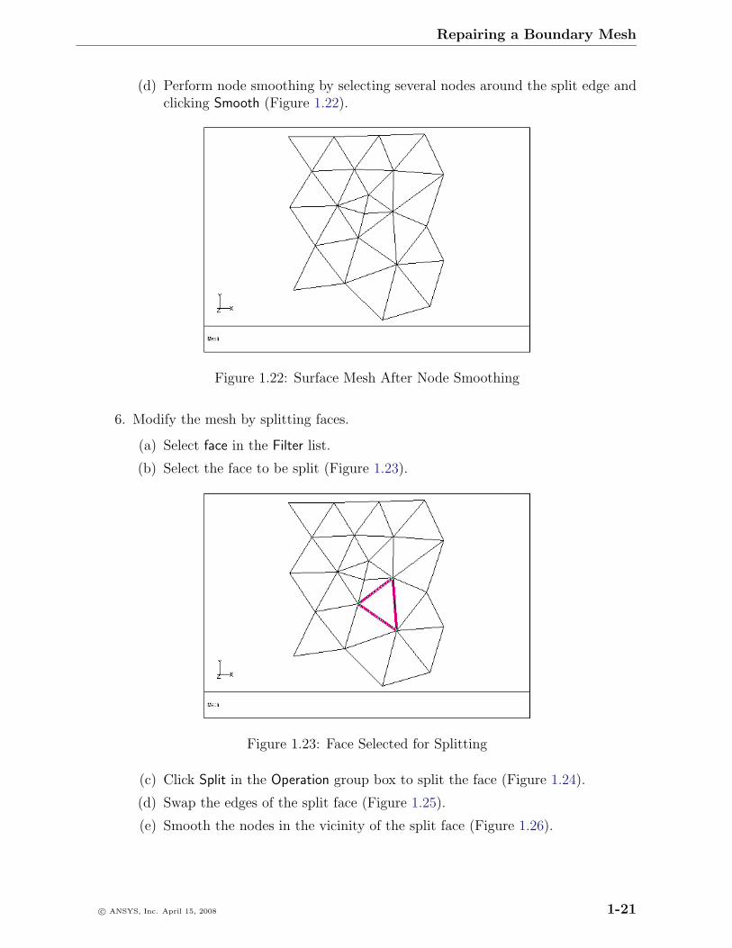
(d) Perform node smoothing by selecting several nodes around the split edge andclicking Smooth (Figure 1.22).
Figure 1.22: Surface Mesh After Node Smoothing
6. Modify the mesh by splitting faces.
(a) Select face in the Filter list.
(b) Select the face to be split (Figure 1.23).
Figure 1.23: Face Selected for Splitting
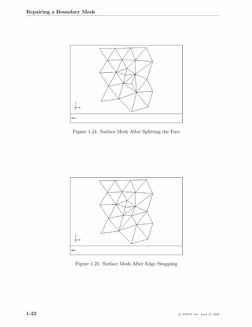
(c) Click Split in the Operation group box to split the face (Figure 1.24).
(d) Swap the edges of the split face (Figure 1.25).
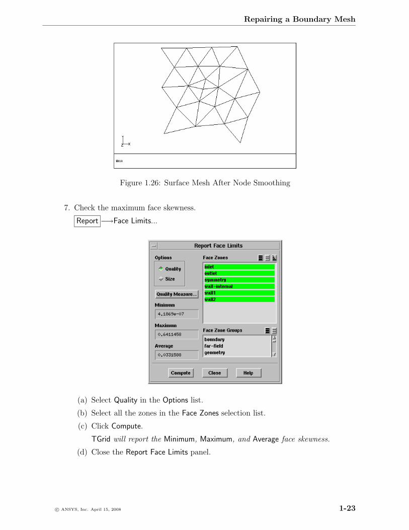
(e) Smooth the nodes in the vicinity of the split face (Figure 1.26).
c© ANSYS, Inc. April 15, 2008 1-21
Repairing a Boundary Mesh
Figure 1.24: Surface Mesh After Splitting the Face
Figure 1.25: Surface Mesh After Edge Swapping
1-22 c© ANSYS, Inc. April 15, 2008
Repairing a Boundary Mesh
Figure 1.26: Surface Mesh After Node Smoothing
7. Check the maximum face skewness.
Report −→Face Limits...
(a) Select Quality in the Options list.
(b) Select all the zones in the Face Zones selection list.
(c) Click Compute.
TGrid will report the Minimum, Maximum, and Average face skewness.
(d) Close the Report Face Limits panel.
c© ANSYS, Inc. April 15, 2008 1-23
Repairing a Boundary Mesh
The maximum face skewness at this point in the tutorial is less than 0.65.There are nine faces with a skewness greater than 0.6 (this information wasobtained from the Face Distribution panel). You can try and reduce the max-imum face skewness to a value less than 0.6 using the face modification toolsdescribed in the previous steps.
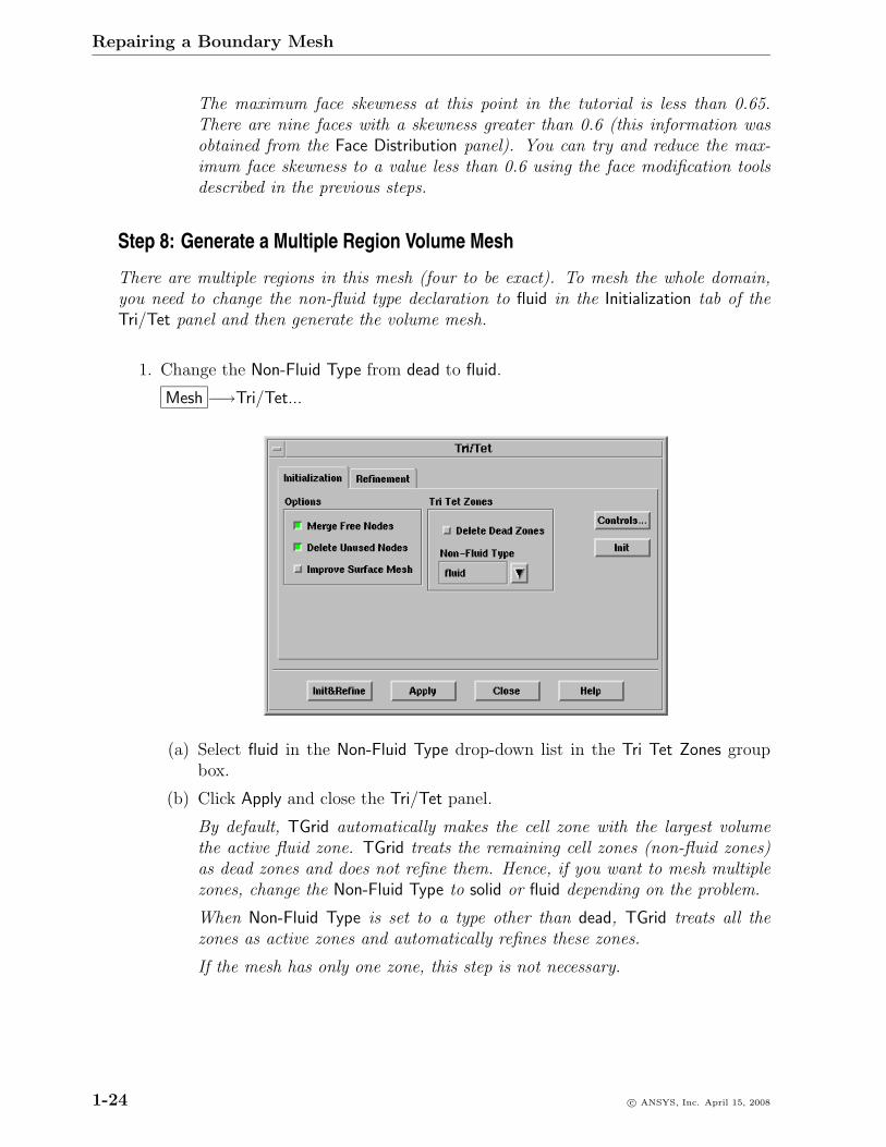
Step 8: Generate a Multiple Region Volume Mesh
There are multiple regions in this mesh (four to be exact). To mesh the whole domain,you need to change the non-fluid type declaration to fluid in the Initialization tab of theTri/Tet panel and then generate the volume mesh.
1. Change the Non-Fluid Type from dead to fluid.
Mesh −→Tri/Tet...
(a) Select fluid in the Non-Fluid Type drop-down list in the Tri Tet Zones groupbox.
(b) Click Apply and close the Tri/Tet panel.
By default, TGrid automatically makes the cell zone with the largest volumethe active fluid zone. TGrid treats the remaining cell zones (non-fluid zones)as dead zones and does not refine them. Hence, if you want to mesh multiplezones, change the Non-Fluid Type to solid or fluid depending on the problem.
When Non-Fluid Type is set to a type other than dead, TGrid treats all thezones as active zones and automatically refines these zones.
If the mesh has only one zone, this step is not necessary.
1-24 c© ANSYS, Inc. April 15, 2008
Repairing a Boundary Mesh
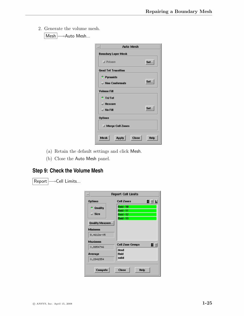
2. Generate the volume mesh.
Mesh −→Auto Mesh...
(a) Retain the default settings and click Mesh.
(b) Close the Auto Mesh panel.
Step 9: Check the Volume Mesh
Report −→Cell Limits...
c© ANSYS, Inc. April 15, 2008 1-25
Repairing a Boundary Mesh
1. Select all the zones in the Cell Zones selection list.
2. Click Compute to report the Maximum, Minimum, and Average cell skewness values.
3. Close the Report Cell Limits panel.
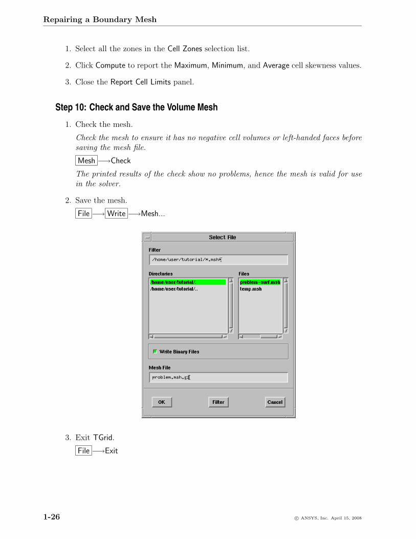
Step 10: Check and Save the Volume Mesh
1. Check the mesh.
Check the mesh to ensure it has no negative cell volumes or left-handed faces beforesaving the mesh file.
Mesh −→Check
The printed results of the check show no problems, hence the mesh is valid for usein the solver.
2. Save the mesh.
File −→ Write −→Mesh...
3. Exit TGrid.
File −→Exit
1-26 c© ANSYS, Inc. April 15, 2008

Repairing a Boundary Mesh
Summary
This tutorial demonstrated the use of some mesh repair tools available in TGrid to fixknown deficiencies in an existing boundary mesh.
c© ANSYS, Inc. April 15, 2008 1-27

Repairing a Boundary Mesh
1-28 c© ANSYS, Inc. April 15, 2008
Tutorial 2. Tetrahedral Mesh Generation
Introduction
The mesh generation process is highly automated in TGrid. In most cases, you can use theAuto Mesh feature to create the volume mesh from the surface mesh. However, in somecases, the boundary mesh may contain irregularities or highly skewed boundary facesthat can lead to an unacceptable volume mesh or cause TGrid to fail while generating theinitial mesh. As a rule of thumb, you need to check the boundary mesh before attemptingto generate the volume mesh. This tutorial demonstrates how to do the following:
• Create a user-defined group for easier selection of boundary sufaces.
• Generate the tetrahedral volume mesh using the various refinement options avail-able in TGrid.
• Compare the mesh generated using the skewness-based and advancing front refine-ment methods.
• Examine the effect of the size function.
• Examine the effect of the maximum cell volume.
• Examine the effect of the growth factor.
• Create a local refinement region.
Prerequisites
This tutorial assumes that you have little experience with TGrid, but that you are familiarwith the graphical user interface.
Preparation
1. Download tet-mesh.zip from the FLUENT User Services Center. This file canbe found from the Documentation link on the TGrid product page.
OR
Copy tet-mesh.zip from the TGrid documentation CD to your working directory.
c© ANSYS, Inc. April 15, 2008 2-1
Tetrahedral Mesh Generation
• For UNIX systems, insert the CD into your CD-ROM drive and go to thefollowing directory:
cdrom/tgrid5.0/help/tutfiles/
where cdrom must be replaced by the name of your CD-ROM drive.
• For Windows systems, insert the CD into your CD-ROM drive and go to thefollowing folder:
cdrom:\tgrid5.0\help\tutfiles\
where, cdrom must be replaced by the name of your CD-ROM drive (e.g., E).
2. Unzip tet-mesh.zip.
The file, sedan.msh.gz can be found in the tet-mesh folder created on unzippingthe file.
3. Start the 3D (3d) version of TGrid.
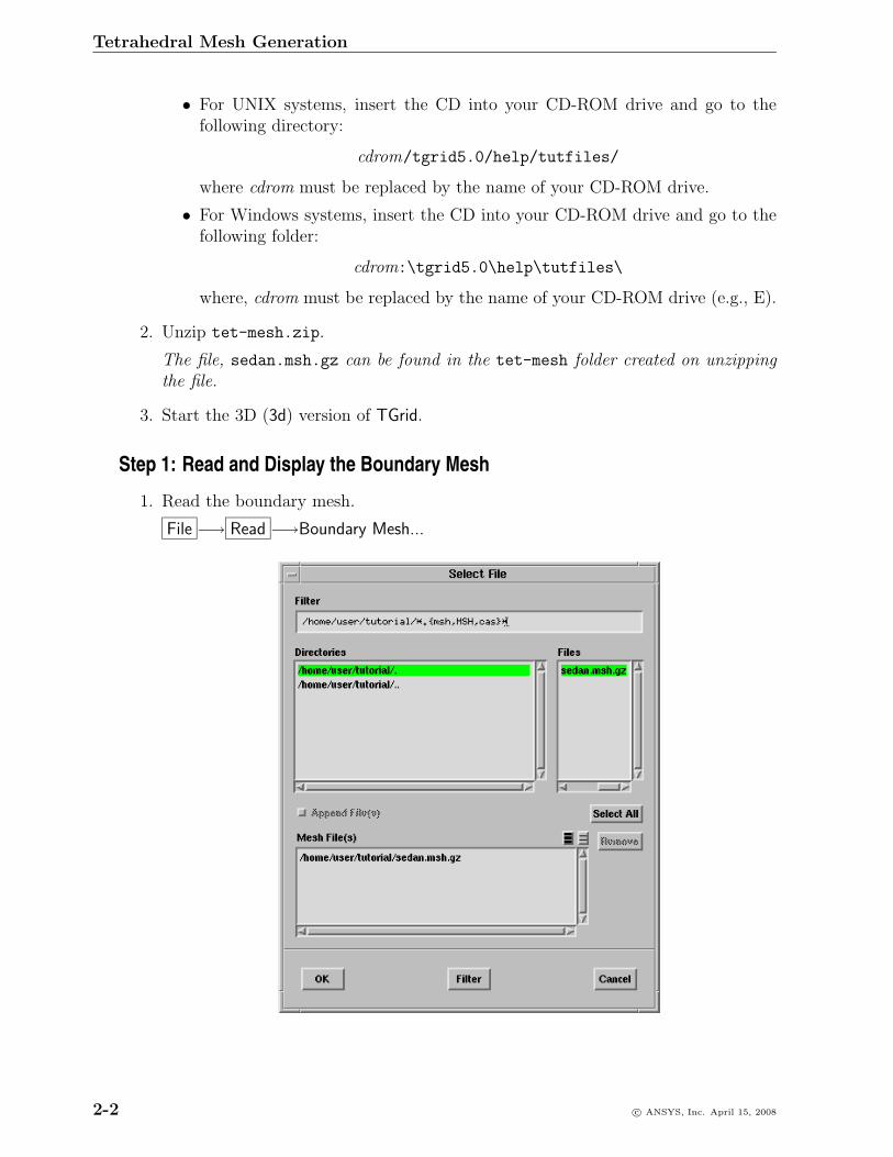
Step 1: Read and Display the Boundary Mesh
1. Read the boundary mesh.
File −→ Read −→Boundary Mesh...
2-2 c© ANSYS, Inc. April 15, 2008
Tetrahedral Mesh Generation
(a) Select sedan.msh.gz in the Files list.
(b) Click OK.
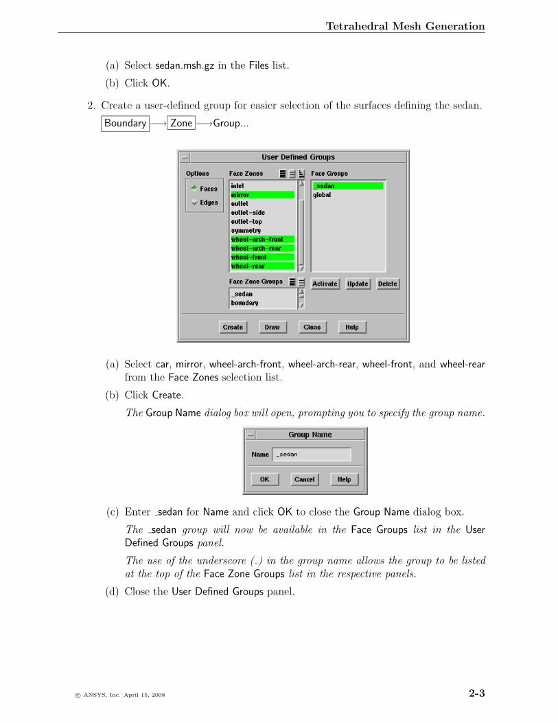
2. Create a user-defined group for easier selection of the surfaces defining the sedan.
Boundary −→ Zone −→Group...
(a) Select car, mirror, wheel-arch-front, wheel-arch-rear, wheel-front, and wheel-rearfrom the Face Zones selection list.
(b) Click Create.
The Group Name dialog box will open, prompting you to specify the group name.
(c) Enter sedan for Name and click OK to close the Group Name dialog box.
The sedan group will now be available in the Face Groups list in the UserDefined Groups panel.
The use of the underscore ( ) in the group name allows the group to be listedat the top of the Face Zone Groups list in the respective panels.
(d) Close the User Defined Groups panel.
c© ANSYS, Inc. April 15, 2008 2-3
Tetrahedral Mesh Generation
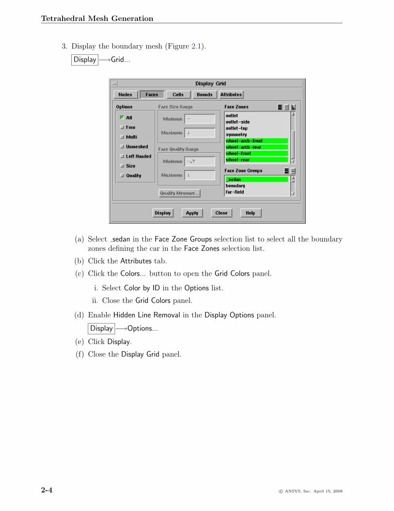
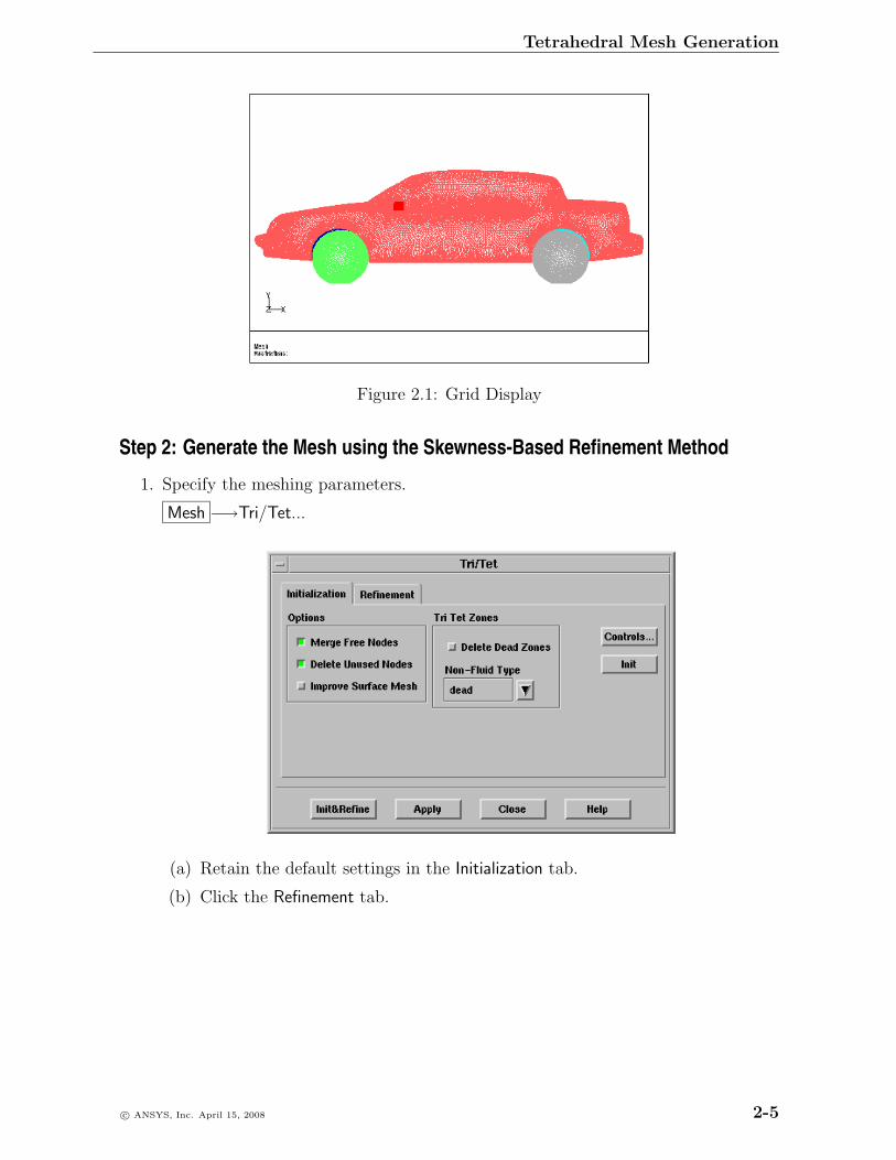
3. Display the boundary mesh (Figure 2.1).
Display −→Grid...
(a) Select sedan in the Face Zone Groups selection list to select all the boundaryzones defining the car in the Face Zones selection list.
(b) Click the Attributes tab.
(c) Click the Colors... button to open the Grid Colors panel.
i. Select Color by ID in the Options list.
ii. Close the Grid Colors panel.
(d) Enable Hidden Line Removal in the Display Options panel.
Display −→Options...
(e) Click Display.
(f) Close the Display Grid panel.
2-4 c© ANSYS, Inc. April 15, 2008
Tetrahedral Mesh Generation
Figure 2.1: Grid Display
Step 2: Generate the Mesh using the Skewness-Based Refinement Method
1. Specify the meshing parameters.
Mesh −→Tri/Tet...
(a) Retain the default settings in the Initialization tab.
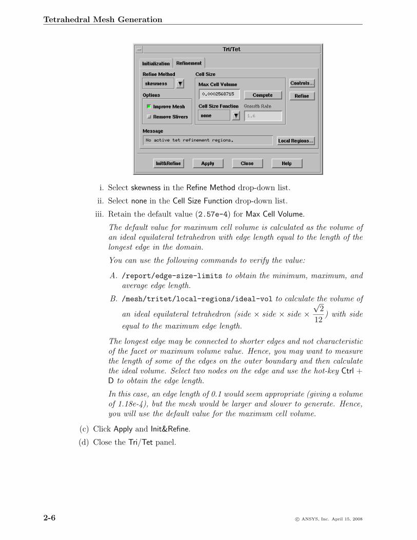
(b) Click the Refinement tab.
c© ANSYS, Inc. April 15, 2008 2-5
Tetrahedral Mesh Generation
i. Select skewness in the Refine Method drop-down list.
ii. Select none in the Cell Size Function drop-down list.
iii. Retain the default value (2.57e-4) for Max Cell Volume.
The default value for maximum cell volume is calculated as the volume ofan ideal equilateral tetrahedron with edge length equal to the length of thelongest edge in the domain.
You can use the following commands to verify the value:
A. /report/edge-size-limits to obtain the minimum, maximum, andaverage edge length.
B. /mesh/tritet/local-regions/ideal-vol to calculate the volume of
an ideal equilateral tetrahedron (side × side × side ×√
2
12) with side
equal to the maximum edge length.
The longest edge may be connected to shorter edges and not characteristicof the facet or maximum volume value. Hence, you may want to measurethe length of some of the edges on the outer boundary and then calculatethe ideal volume. Select two nodes on the edge and use the hot-key Ctrl +D to obtain the edge length.
In this case, an edge length of 0.1 would seem appropriate (giving a volumeof 1.18e-4), but the mesh would be larger and slower to generate. Hence,you will use the default value for the maximum cell volume.
(c) Click Apply and Init&Refine.
(d) Close the Tri/Tet panel.
2-6 c© ANSYS, Inc. April 15, 2008
Tetrahedral Mesh Generation
2. Examine the mesh.
Display −→Grid...
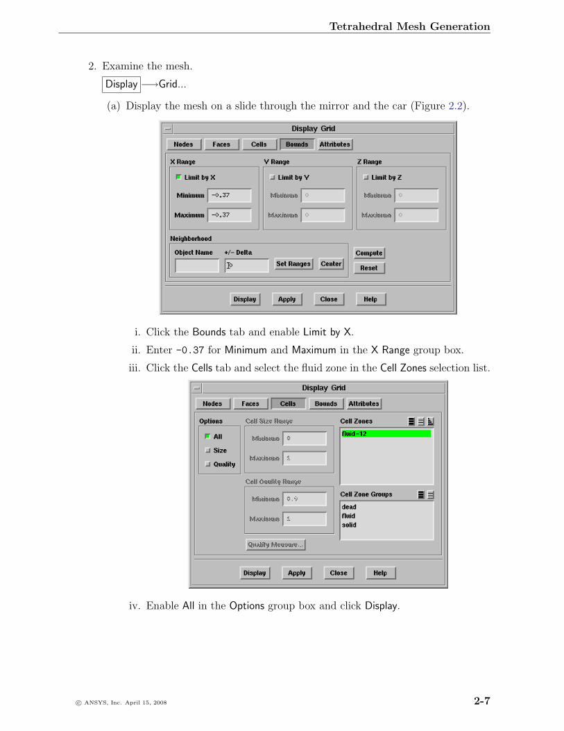
(a) Display the mesh on a slide through the mirror and the car (Figure 2.2).
i. Click the Bounds tab and enable Limit by X.
ii. Enter -0.37 for Minimum and Maximum in the X Range group box.
iii. Click the Cells tab and select the fluid zone in the Cell Zones selection list.
iv. Enable All in the Options group box and click Display.
c© ANSYS, Inc. April 15, 2008 2-7
Tetrahedral Mesh Generation
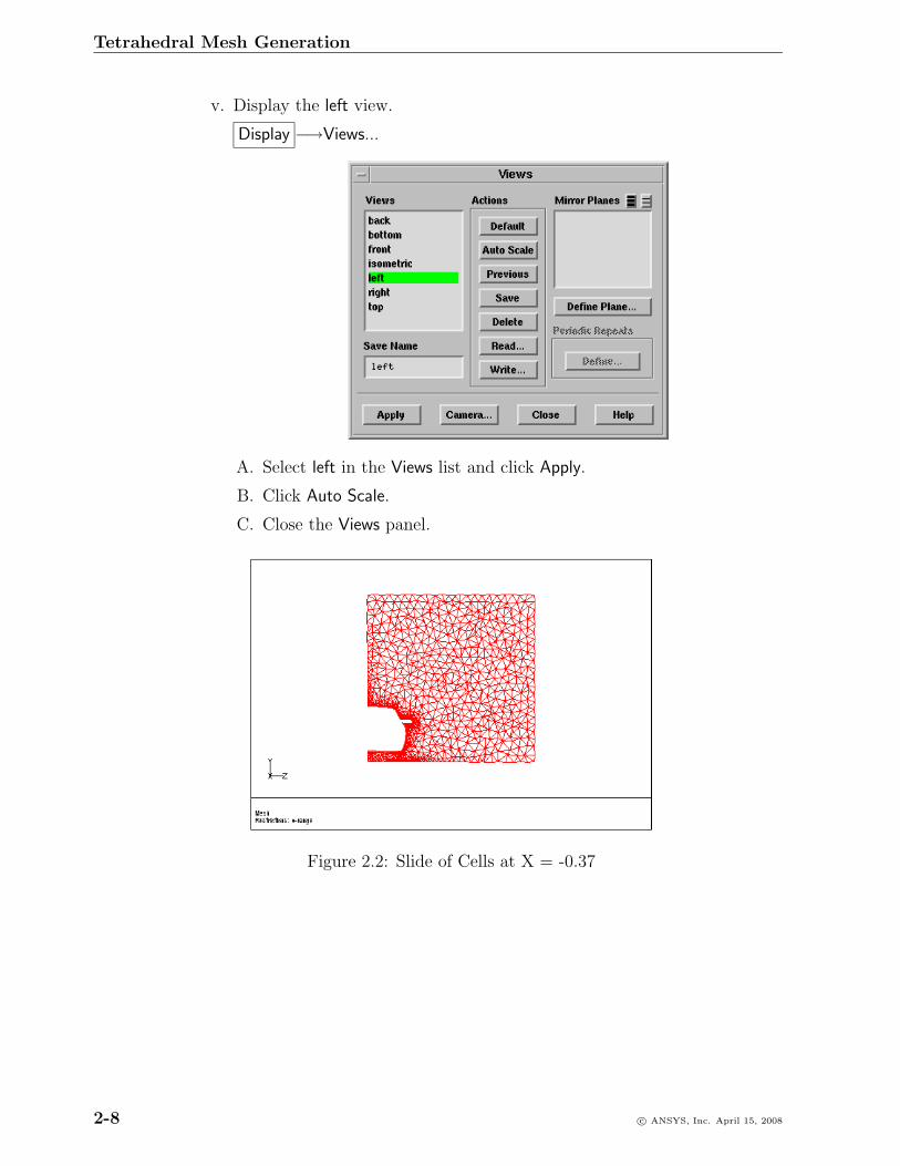
v. Display the left view.
Display −→Views...
A. Select left in the Views list and click Apply.
B. Click Auto Scale.
C. Close the Views panel.
Figure 2.2: Slide of Cells at X = -0.37
2-8 c© ANSYS, Inc. April 15, 2008
Tetrahedral Mesh Generation
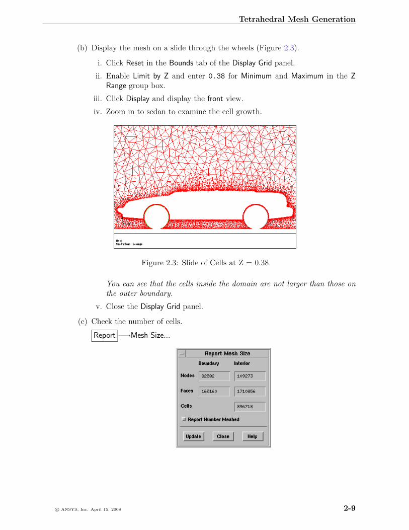
(b) Display the mesh on a slide through the wheels (Figure 2.3).
i. Click Reset in the Bounds tab of the Display Grid panel.
ii. Enable Limit by Z and enter 0.38 for Minimum and Maximum in the ZRange group box.
iii. Click Display and display the front view.
iv. Zoom in to sedan to examine the cell growth.
Figure 2.3: Slide of Cells at Z = 0.38
You can see that the cells inside the domain are not larger than those onthe outer boundary.
v. Close the Display Grid panel.
(c) Check the number of cells.
Report −→Mesh Size...
c© ANSYS, Inc. April 15, 2008 2-9
Tetrahedral Mesh Generation
i. Click Update.
The number of cells is 896718. The exact number may differ on differentplatforms.
ii. Close the Report Mesh Size panel.
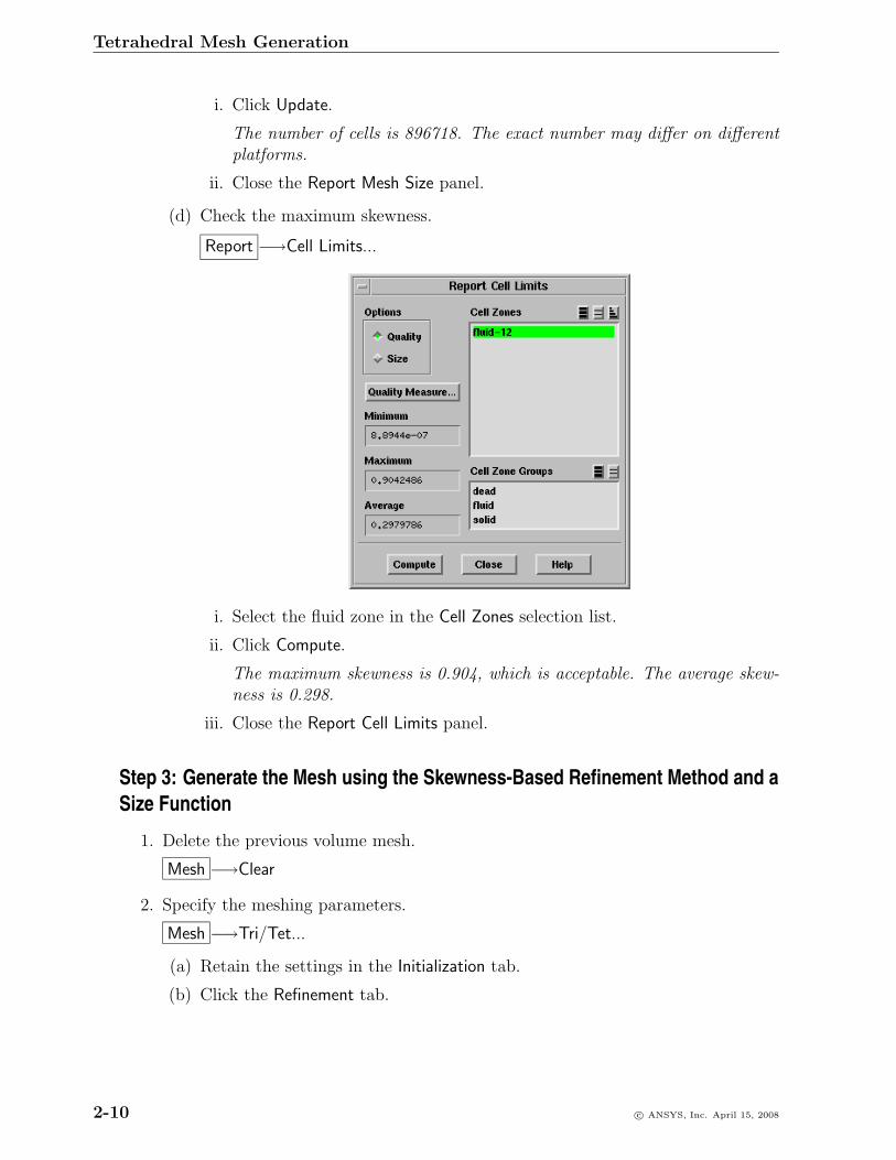
(d) Check the maximum skewness.
Report −→Cell Limits...
i. Select the fluid zone in the Cell Zones selection list.
ii. Click Compute.
The maximum skewness is 0.904, which is acceptable. The average skew-ness is 0.298.
iii. Close the Report Cell Limits panel.
Step 3: Generate the Mesh using the Skewness-Based Refinement Method and aSize Function
1. Delete the previous volume mesh.
Mesh −→Clear
2. Specify the meshing parameters.
Mesh −→Tri/Tet...
(a) Retain the settings in the Initialization tab.
(b) Click the Refinement tab.
2-10 c© ANSYS, Inc. April 15, 2008
Tetrahedral Mesh Generation
i. Retain the selection of skewness in the Refine Method drop-down list.
ii. Select geometric in the Cell Size Function drop-down list and enter 1.3 forGrowth Rate.
iii. Retain the default value (2.57e-4) for Max Cell Volume.
iv. Click Apply and Init&Refine.
v. Close the Tri/Tet panel.
(c) Examine the mesh.
Display −→Grid...
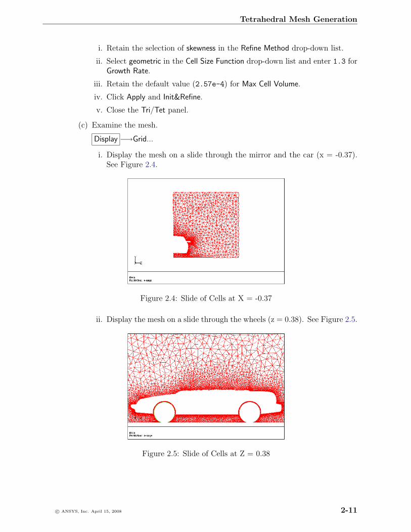
i. Display the mesh on a slide through the mirror and the car (x = -0.37).See Figure 2.4.
Figure 2.4: Slide of Cells at X = -0.37
ii. Display the mesh on a slide through the wheels (z = 0.38). See Figure 2.5.
Figure 2.5: Slide of Cells at Z = 0.38
c© ANSYS, Inc. April 15, 2008 2-11

Tetrahedral Mesh Generation
(d) Check the number of cells.
Report −→Mesh Size...
The number of cells is 1658326. The exact number may differ on differentplatforms.
(e) Check the maximum skewness.
Report −→Cell Limits...
The maximum skewness is 0.904, which is acceptable. The average skewnessis 0.249.
You can see that the transition between small and large cells is smoother than thatfor the previous mesh. The transition is smoother when the specified growth rate iscloser to 1.
Step 4: Generate the Mesh using the Advancing Front Refinement Method and aSize Function
1. Delete the previous volume mesh.
Mesh −→Clear
2. Specify the meshing parameters.
Mesh −→Tri/Tet...
(a) Retain the settings in the Initialization tab.
(b) Click the Refinement tab.
i. Select adv-front in the Refine Method drop-down list.
ii. Retain the selection of geometric in the Cell Size Function drop-down listand retain 1.3 for Growth Rate.
iii. Retain the default value (2.57e-4) for Max Cell Volume.
iv. Click Apply and Init&Refine.
v. Close the Tri/Tet panel.
(c) Examine the mesh.
Display −→Grid...
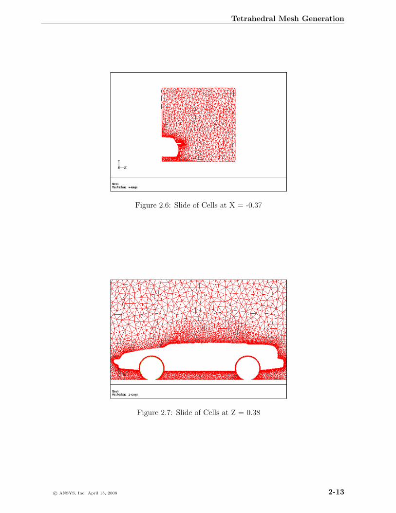
i. Display the mesh on a slide through the mirror and the car (x = -0.37).See Figure 2.6.
ii. Display the mesh on a slide through the wheels (z = 0.38). See Figure 2.7.
2-12 c© ANSYS, Inc. April 15, 2008
Tetrahedral Mesh Generation
Figure 2.6: Slide of Cells at X = -0.37
Figure 2.7: Slide of Cells at Z = 0.38
c© ANSYS, Inc. April 15, 2008 2-13
Tetrahedral Mesh Generation
(d) Check the number of cells.
Report −→Mesh Size...
The number of cells is 1493701. The exact number may differ on differentplatforms.
(e) Check the maximum skewness.
Report −→Cell Limits...
The maximum skewness is 0.904, which is acceptable. The average skewnessis 0.245.
(f) Examine the cell size distribution.
Display −→ Plot −→Cell Distribution...
i. Select the fluid zone in the Cell Zones selection list.
ii. Select Size from the Options list and click Compute.
The maximum cell volume is 2.23e-4.
Note: The maximum cell volume (2.23e-4) is lower than the specifiedvalue (2.57e-4).
iii. Close the Cell Distribution panel.
• The quality is very similar to that obtained with the skewness-based refinementalgorithm. Generally, the maximum skewness will be similar for both refine-ment methods, but the average skewness will be better with the advancing frontmethod.
• The maximum cell volume criterion is well respected. In the middle of thedomain, the cell volume is defined by that parameter. However, a few cellsmay still be above the specified size since quality is predominant on the size.
• As far as the number of cells is concerned, for a strict volume criterion, theadvancing front method will generate more cells, but for a relaxed maximumvolume criterion, the skewness method will generate more cells. .
• For a mesh of size similar to that considered in this tutorial, tet refinement forthe advancing front method is approximately 1.8 times faster when comparedwith the skewness method. The speedup will increase for bigger size meshes.
2-14 c© ANSYS, Inc. April 15, 2008
Tetrahedral Mesh Generation
Step 5: Examine the Effect of the Maximum Cell Volume
1. Clear the mesh.
2. Specify the meshing parameters.
Mesh −→Tri/Tet...
(a) Retain the selection of adv-front in the Refine Method drop-down list and theGrowth Rate of 1.3, respectively.
(b) Enter 2e-2 for Max Cell Volume in the Refinement tab of the Tri/Tet panel.
(c) Click Apply and Init&Refine.
(d) Close the Tri/Tet panel.
3. Examine the mesh.
Display −→Grid...
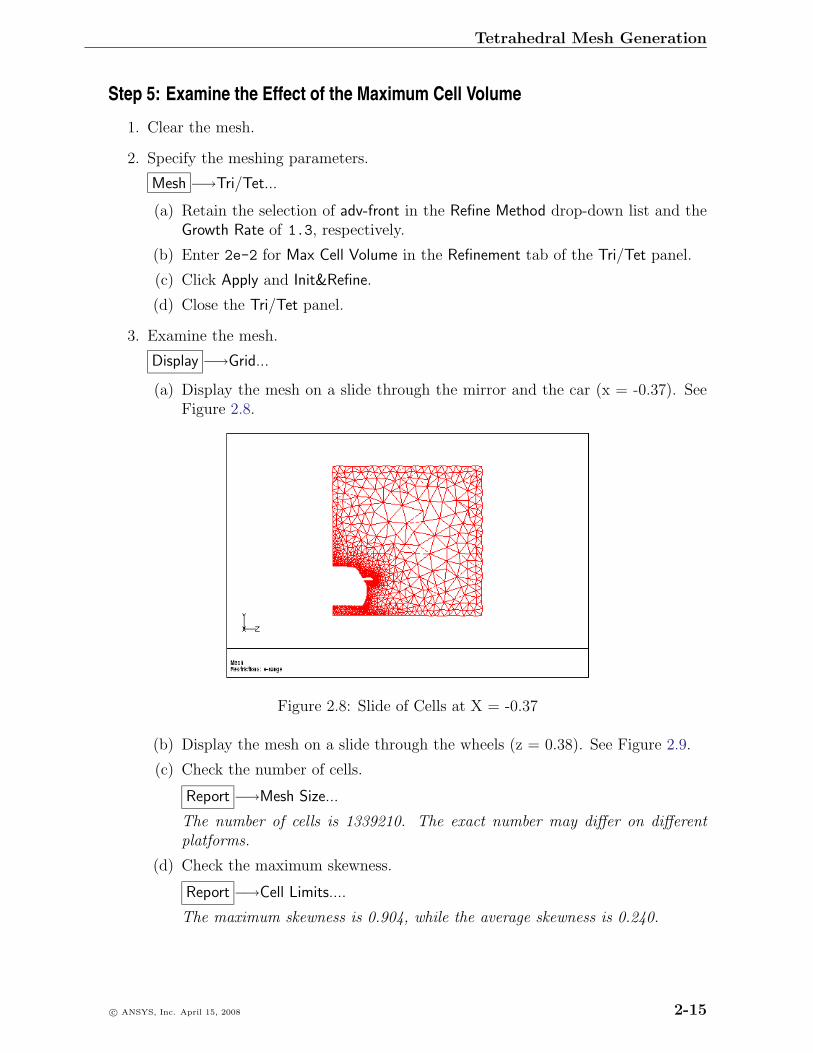
(a) Display the mesh on a slide through the mirror and the car (x = -0.37). SeeFigure 2.8.
Figure 2.8: Slide of Cells at X = -0.37
(b) Display the mesh on a slide through the wheels (z = 0.38). See Figure 2.9.
(c) Check the number of cells.
Report −→Mesh Size...
The number of cells is 1339210. The exact number may differ on differentplatforms.
(d) Check the maximum skewness.
Report −→Cell Limits....
The maximum skewness is 0.904, while the average skewness is 0.240.
c© ANSYS, Inc. April 15, 2008 2-15
Tetrahedral Mesh Generation
Figure 2.9: Slide of Cells at Z = 0.38
(e) Check the maximum cell volume.
Report −→Cell Limits...
i. Select the fluid zone in the Cell Zones selection list.
ii. Select Size from the Options list and click Compute.
The maximum cell volume is 4.69e-3 which is lower than the specifiedvalue (2e-2). For the mesh generated, the maximum cell volume is lowerthan the value specified, indicating that the size distribution was based onthe surface mesh, the growth rate, and the quality, and not restricted bythe maximum cell volume specified. Hence, the edge length of the cells inthe centre of the domain is more than the edge length of the cells on theboundary.
Step 6: Examine the Effect of the Growth Factor
1. Clear the mesh.
2. Specify the meshing parameters.
Mesh −→Tri/Tet...
(a) Retain the selection of adv-front in the Refine Method drop-down list and theMax Cell Volume of 2e-2, respectively.
(b) Enter 1.25 for Growth Rate in the Refinement tab of the Tri/Tet panel.
(c) Click Apply and Init&Refine.
(d) Close the Tri/Tet panel.
2-16 c© ANSYS, Inc. April 15, 2008
Tetrahedral Mesh Generation
3. Examine the mesh.
Display −→Grid...
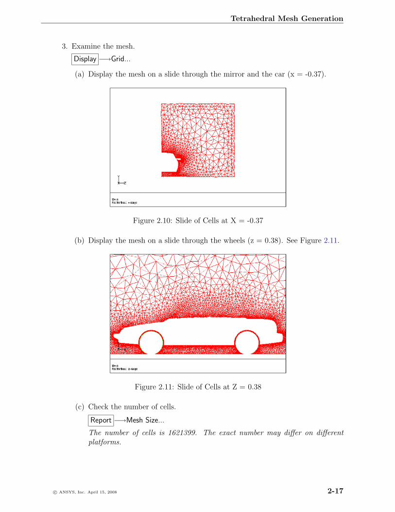
(a) Display the mesh on a slide through the mirror and the car (x = -0.37).
Figure 2.10: Slide of Cells at X = -0.37
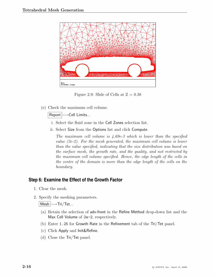
(b) Display the mesh on a slide through the wheels (z = 0.38). See Figure 2.11.
Figure 2.11: Slide of Cells at Z = 0.38
(c) Check the number of cells.
Report −→Mesh Size...
The number of cells is 1621399. The exact number may differ on differentplatforms.
c© ANSYS, Inc. April 15, 2008 2-17
Tetrahedral Mesh Generation
(d) Check the maximum skewness.
Report −→Cell Limits...
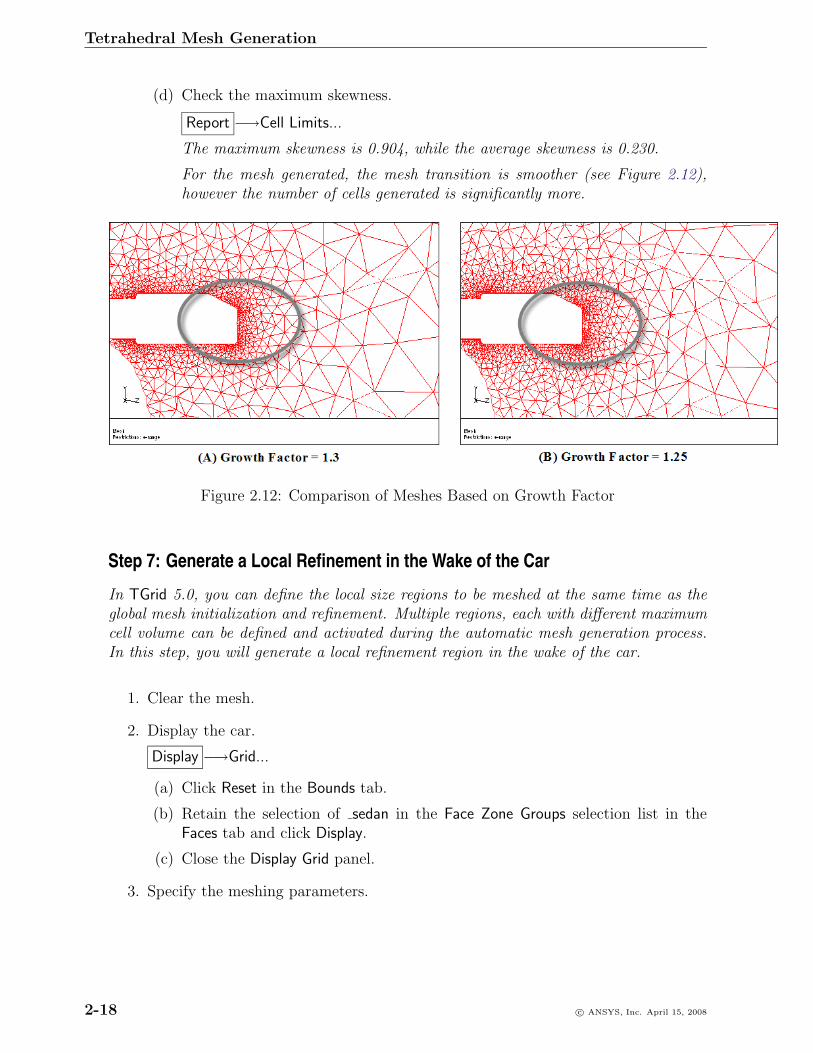
The maximum skewness is 0.904, while the average skewness is 0.230.
For the mesh generated, the mesh transition is smoother (see Figure 2.12),however the number of cells generated is significantly more.
Figure 2.12: Comparison of Meshes Based on Growth Factor
Step 7: Generate a Local Refinement in the Wake of the Car
In TGrid 5.0, you can define the local size regions to be meshed at the same time as theglobal mesh initialization and refinement. Multiple regions, each with different maximumcell volume can be defined and activated during the automatic mesh generation process.In this step, you will generate a local refinement region in the wake of the car.
1. Clear the mesh.
2. Display the car.
Display −→Grid...
(a) Click Reset in the Bounds tab.
(b) Retain the selection of sedan in the Face Zone Groups selection list in theFaces tab and click Display.
(c) Close the Display Grid panel.
3. Specify the meshing parameters.
2-18 c© ANSYS, Inc. April 15, 2008
Tetrahedral Mesh Generation
(a) Retain the previous settings in the Initialization tab of the Tri/Tet panel.
Mesh −→Tri/Tet...
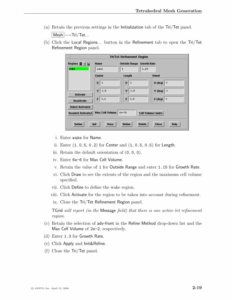
(b) Click the Local Regions... button in the Refinement tab to open the Tri/TetRefinement Region panel.
i. Enter wake for Name.
ii. Enter (1, 0.5, 0.2) for Center and (1, 0.5, 0.5) for Length.
iii. Retain the default orientation of (0, 0, 0).
iv. Enter 6e-6 for Max Cell Volume.
v. Retain the value of 1 for Outside Range and enter 1.15 for Growth Rate.
vi. Click Draw to see the extents of the region and the maximum cell volumespecified.
vii. Click Define to define the wake region.
viii. Click Activate for the region to be taken into account during refinement.
ix. Close the Tri/Tet Refinement Region panel.
TGrid will report (in the Message field) that there is one active tet refinementregion.
(c) Retain the selection of adv-front in the Refine Method drop-down list and theMax Cell Volume of 2e-2, respectively.
(d) Enter 1.3 for Growth Rate.
(e) Click Apply and Init&Refine.
(f) Close the Tri/Tet panel.
c© ANSYS, Inc. April 15, 2008 2-19
Tetrahedral Mesh Generation
4. Examine the mesh.
Display −→Grid...
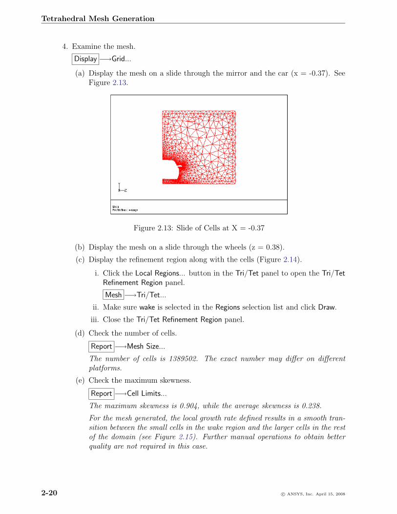
(a) Display the mesh on a slide through the mirror and the car (x = -0.37). SeeFigure 2.13.
Figure 2.13: Slide of Cells at X = -0.37
(b) Display the mesh on a slide through the wheels (z = 0.38).
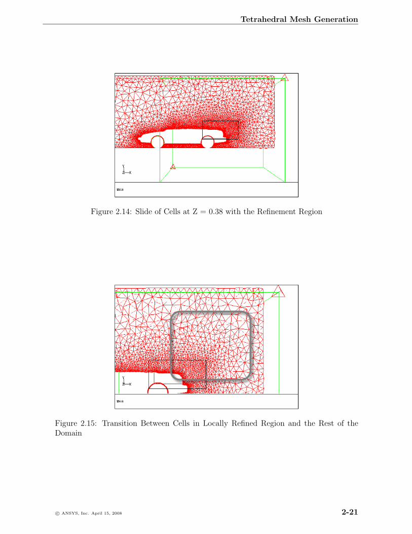
(c) Display the refinement region along with the cells (Figure 2.14).
i. Click the Local Regions... button in the Tri/Tet panel to open the Tri/TetRefinement Region panel.
Mesh −→Tri/Tet...
ii. Make sure wake is selected in the Regions selection list and click Draw.
iii. Close the Tri/Tet Refinement Region panel.
(d) Check the number of cells.
Report −→Mesh Size...
The number of cells is 1389502. The exact number may differ on differentplatforms.
(e) Check the maximum skewness.
Report −→Cell Limits...
The maximum skewness is 0.904, while the average skewness is 0.238.
For the mesh generated, the local growth rate defined results in a smooth tran-sition between the small cells in the wake region and the larger cells in the restof the domain (see Figure 2.15). Further manual operations to obtain betterquality are not required in this case.
2-20 c© ANSYS, Inc. April 15, 2008
Tetrahedral Mesh Generation
Figure 2.14: Slide of Cells at Z = 0.38 with the Refinement Region
Figure 2.15: Transition Between Cells in Locally Refined Region and the Rest of theDomain
c© ANSYS, Inc. April 15, 2008 2-21
Tetrahedral Mesh Generation
Step 8: Check and Save the Volume Mesh
1. Check the mesh.
Mesh −→Check
TGrid will perform various checks on the mesh and report the progress in the console.Make sure the minimum volume reported is a positive number.
2. Save the mesh.
File −→ Write −→Mesh...
(a) Enter sedan-vol.msh.gz for Mesh File.
(b) Click OK to save the volume mesh.
3. Exit TGrid.
File −→Exit
Summary
This tutorial demonstrated the tetrahedral mesh generation process using both the re-finement methods available in TGrid. It also examined the effect of the size function,maximum cell volume, and the growth factor on the generated mesh. The quality ofthe mesh generated is similar for both the refinement methods available. However, formost cases, the advancing front method will be faster due to a greater number of cellsgenerated per second. The use of local refinement regions was also demonstrated.
2-22 c© ANSYS, Inc. April 15, 2008
Tutorial 3. Zonal Hybrid Mesh Generation
Introduction
There are many cases in which you may use hexahedral cells to mesh one part of yourgeometry, but complexities in another part of the geometry require that it be meshedwith tetrahedral cells. In such cases, you can use the usual preprocessor to create themixed triangular surface mesh and the hexahedral volume mesh, and then use TGrid tocomplete the hybrid mesh generation.
This tutorial demonstrates the mesh generation procedure for a hybrid mesh, startingfrom a hexahedral volume mesh and a triangular boundary mesh. This tutorial demon-strates how to do the following:
1. Read the mesh files and display the boundary mesh.
2. Merge the free nodes on the two pieces of the mesh (hexahedral volume mesh andtriangular boundary mesh).
3. Create pyramids as a transition between the hexahedral and tetrahedral mesh usingthe Auto Mesh procedure.
4. Build prisms from the bottom of the tetrahedral region.
5. Check the quality of the entire volume mesh.
6. Merge the multiple cell zones into a single cell zone.
7. Create a non-conformal interface as a transition between the hexahedral and tetra-hedral mesh using the Auto Mesh procedure.
Prerequisites
This tutorial assumes that you have little experience with TGrid, but that you are familiarwith the graphical user interface.
c© ANSYS, Inc. April 15, 2008 3-1
Zonal Hybrid Mesh Generation
Preparation
1. Download zonal-hybrid.zip from the FLUENT User Services Center to yourworking directory. This file can be found from the Documentation link on theTGrid product page.
OR
Copy zonal-hybrid.zip from the TGrid documentation CD to your working di-rectory.
• For UNIX systems, insert the CD into your CD-ROM drive and go to thefollowing directory:
cdrom/tgrid5.0/help/tutfiles/
where, cdrom must be replaced by the name of your CD-ROM drive.
• For Windows systems, insert the CD into your CD-ROM drive and go to thefollowing folder:
cdrom:\tgrid5.0\help\tutfiles
where, cdrom must be replaced by the name of your CD-ROM drive (e.g., E).
2. Unzip zonal-hybrid.zip.
The files, hex-vol.msh and tri-srf.msh can be found in the zonal-hybrid foldercreated on unzipping the file.
3. Start the 3D (3d) version of TGrid.
3-2 c© ANSYS, Inc. April 15, 2008
Zonal Hybrid Mesh Generation
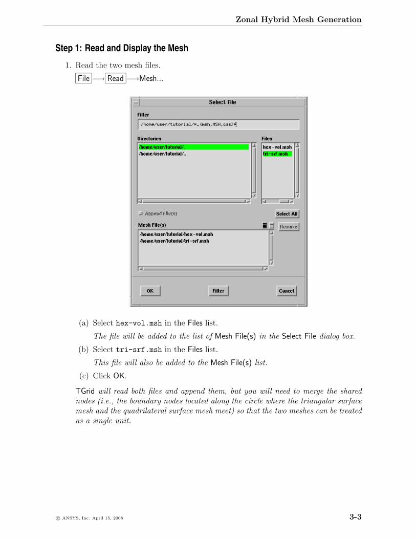
Step 1: Read and Display the Mesh
1. Read the two mesh files.
File −→ Read −→Mesh...
(a) Select hex-vol.msh in the Files list.
The file will be added to the list of Mesh File(s) in the Select File dialog box.
(b) Select tri-srf.msh in the Files list.
This file will also be added to the Mesh File(s) list.
(c) Click OK.
TGrid will read both files and append them, but you will need to merge the sharednodes (i.e., the boundary nodes located along the circle where the triangular surfacemesh and the quadrilateral surface mesh meet) so that the two meshes can be treatedas a single unit.
c© ANSYS, Inc. April 15, 2008 3-3
Zonal Hybrid Mesh Generation
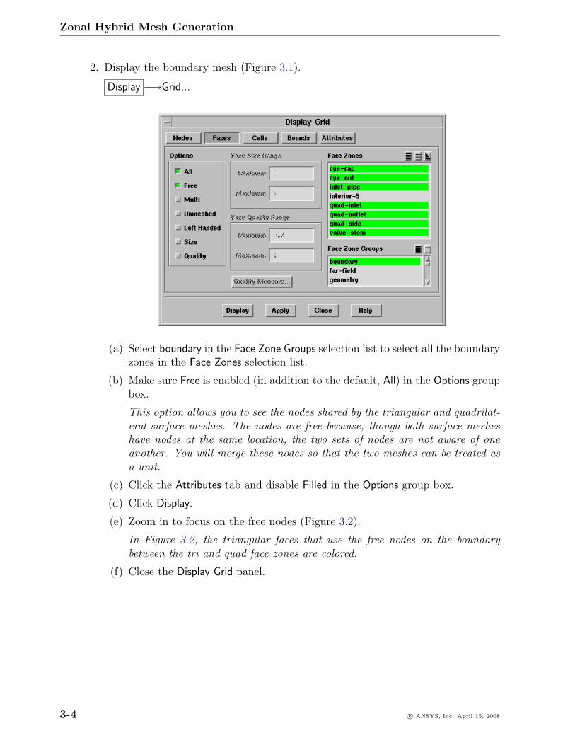
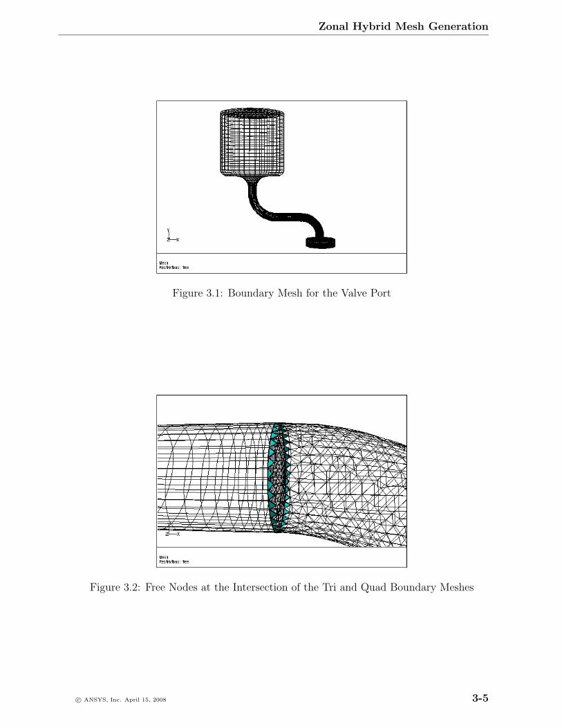
2. Display the boundary mesh (Figure 3.1).
Display −→Grid...
(a) Select boundary in the Face Zone Groups selection list to select all the boundaryzones in the Face Zones selection list.
(b) Make sure Free is enabled (in addition to the default, All) in the Options groupbox.
This option allows you to see the nodes shared by the triangular and quadrilat-eral surface meshes. The nodes are free because, though both surface mesheshave nodes at the same location, the two sets of nodes are not aware of oneanother. You will merge these nodes so that the two meshes can be treated asa unit.
(c) Click the Attributes tab and disable Filled in the Options group box.
(d) Click Display.
(e) Zoom in to focus on the free nodes (Figure 3.2).
In Figure 3.2, the triangular faces that use the free nodes on the boundarybetween the tri and quad face zones are colored.
(f) Close the Display Grid panel.
3-4 c© ANSYS, Inc. April 15, 2008
Zonal Hybrid Mesh Generation
Figure 3.1: Boundary Mesh for the Valve Port
Figure 3.2: Free Nodes at the Intersection of the Tri and Quad Boundary Meshes
c© ANSYS, Inc. April 15, 2008 3-5
Zonal Hybrid Mesh Generation
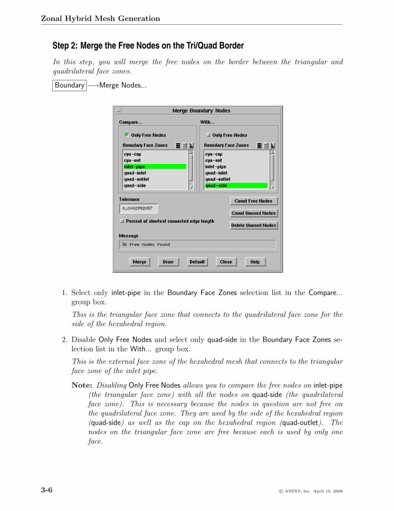
Step 2: Merge the Free Nodes on the Tri/Quad Border
In this step, you will merge the free nodes on the border between the triangular andquadrilateral face zones.
Boundary −→Merge Nodes...
1. Select only inlet-pipe in the Boundary Face Zones selection list in the Compare...group box.
This is the triangular face zone that connects to the quadrilateral face zone for theside of the hexahedral region.
2. Disable Only Free Nodes and select only quad-side in the Boundary Face Zones se-lection list in the With... group box.
This is the external face zone of the hexahedral mesh that connects to the triangularface zone of the inlet pipe.
Note: Disabling Only Free Nodes allows you to compare the free nodes on inlet-pipe(the triangular face zone) with all the nodes on quad-side (the quadrilateralface zone). This is necessary because the nodes in question are not free onthe quadrilateral face zone. They are used by the side of the hexahedral region(quad-side) as well as the cap on the hexahedral region (quad-outlet). Thenodes on the triangular face zone are free because each is used by only oneface.
3-6 c© ANSYS, Inc. April 15, 2008
Zonal Hybrid Mesh Generation
After you merge the free nodes, the nodes of the triangular face will be con-nected to quad-outlet and quad-side.
3. Click Count Free Nodes.
TGrid will report the number of free nodes in the Message box.
4. Click Merge to merge the free nodes.
When the number of merged nodes is reported, not all of the free nodes were merged.This implies that some of the nodes differ from their counterparts by a distancegreater than the specified Tolerance. Increase the Tolerance by a factor of 10 andtry the merge operation again.
5. Enter 0.002992057 for Tolerance.
6. Click Merge.
The remaining nodes should now be merged.
7. Click Count Free Nodes again to ensure that all the free nodes have been merged.
8. Close the Merge Boundary Nodes panel.
9. Save the mesh file.
File −→ Write −→Mesh...
(a) Enter hex-tri-merged.msh for Mesh File.
(b) Click OK to save the mesh.
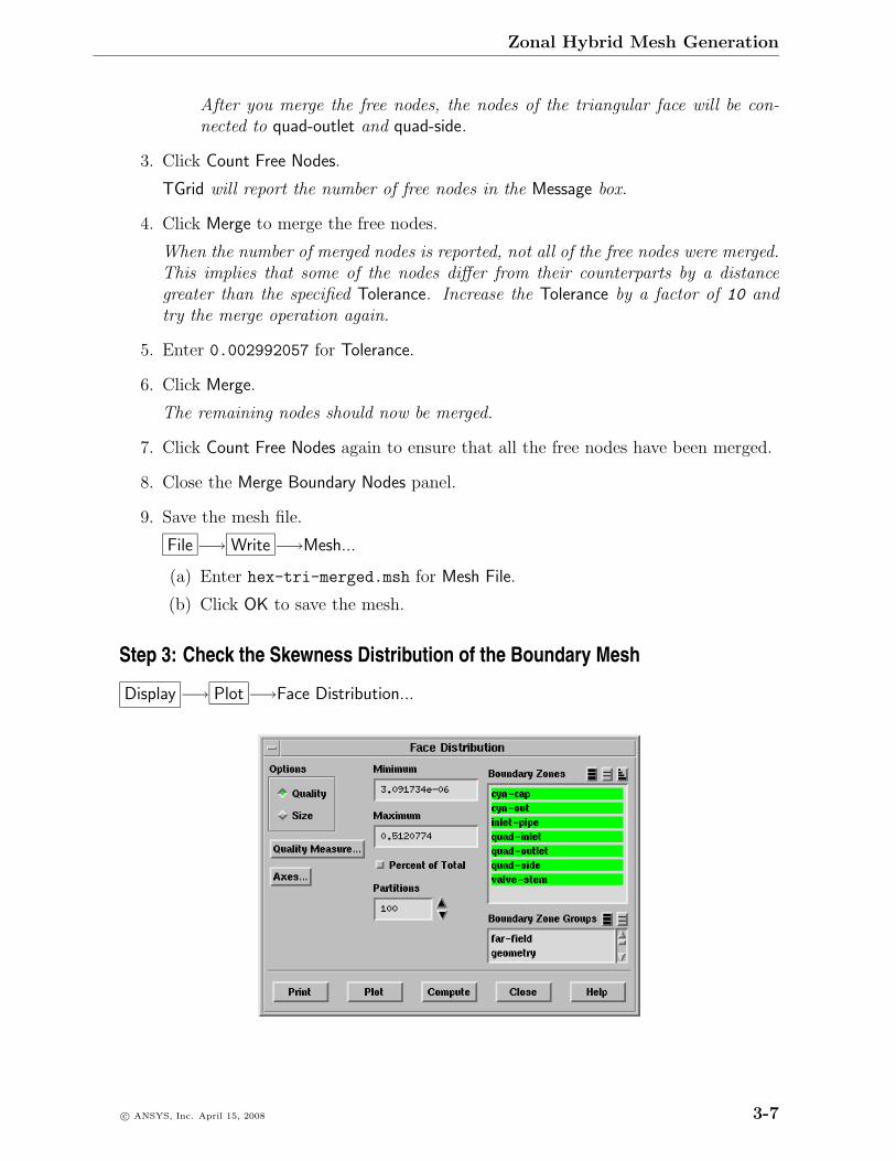
Step 3: Check the Skewness Distribution of the Boundary Mesh
Display −→ Plot −→Face Distribution...
c© ANSYS, Inc. April 15, 2008 3-7
Zonal Hybrid Mesh Generation
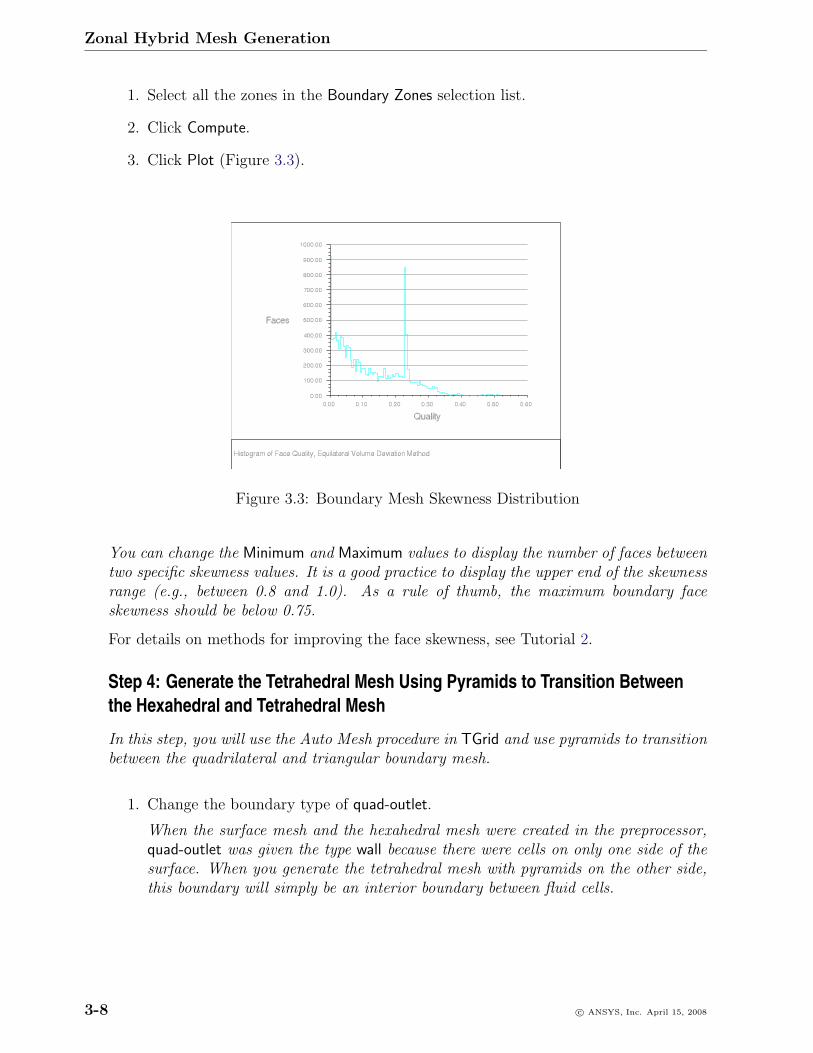
1. Select all the zones in the Boundary Zones selection list.
2. Click Compute.
3. Click Plot (Figure 3.3).
Figure 3.3: Boundary Mesh Skewness Distribution
You can change the Minimum and Maximum values to display the number of faces betweentwo specific skewness values. It is a good practice to display the upper end of the skewnessrange (e.g., between 0.8 and 1.0). As a rule of thumb, the maximum boundary faceskewness should be below 0.75.
For details on methods for improving the face skewness, see Tutorial 2.
Step 4: Generate the Tetrahedral Mesh Using Pyramids to Transition Betweenthe Hexahedral and Tetrahedral Mesh
In this step, you will use the Auto Mesh procedure in TGrid and use pyramids to transitionbetween the quadrilateral and triangular boundary mesh.
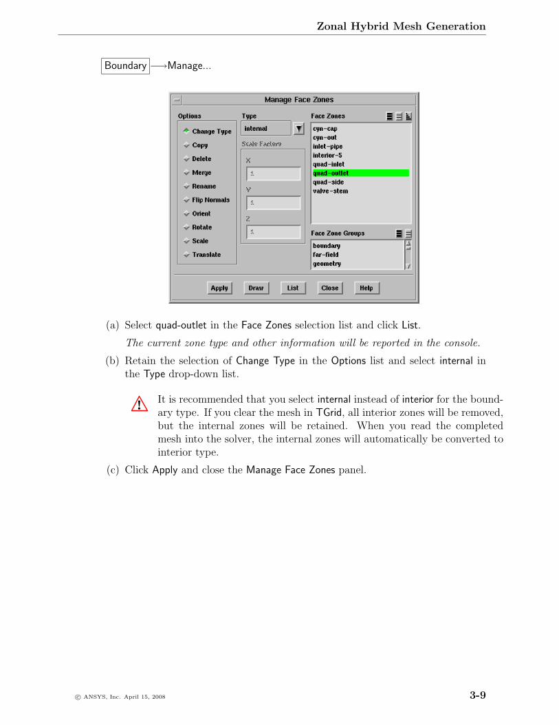
1. Change the boundary type of quad-outlet.
When the surface mesh and the hexahedral mesh were created in the preprocessor,quad-outlet was given the type wall because there were cells on only one side of thesurface. When you generate the tetrahedral mesh with pyramids on the other side,this boundary will simply be an interior boundary between fluid cells.
3-8 c© ANSYS, Inc. April 15, 2008
Zonal Hybrid Mesh Generation
Boundary −→Manage...
(a) Select quad-outlet in the Face Zones selection list and click List.
The current zone type and other information will be reported in the console.
(b) Retain the selection of Change Type in the Options list and select internal inthe Type drop-down list.
! It is recommended that you select internal instead of interior for the bound-ary type. If you clear the mesh in TGrid, all interior zones will be removed,but the internal zones will be retained. When you read the completedmesh into the solver, the internal zones will automatically be converted tointerior type.
(c) Click Apply and close the Manage Face Zones panel.
c© ANSYS, Inc. April 15, 2008 3-9
Zonal Hybrid Mesh Generation
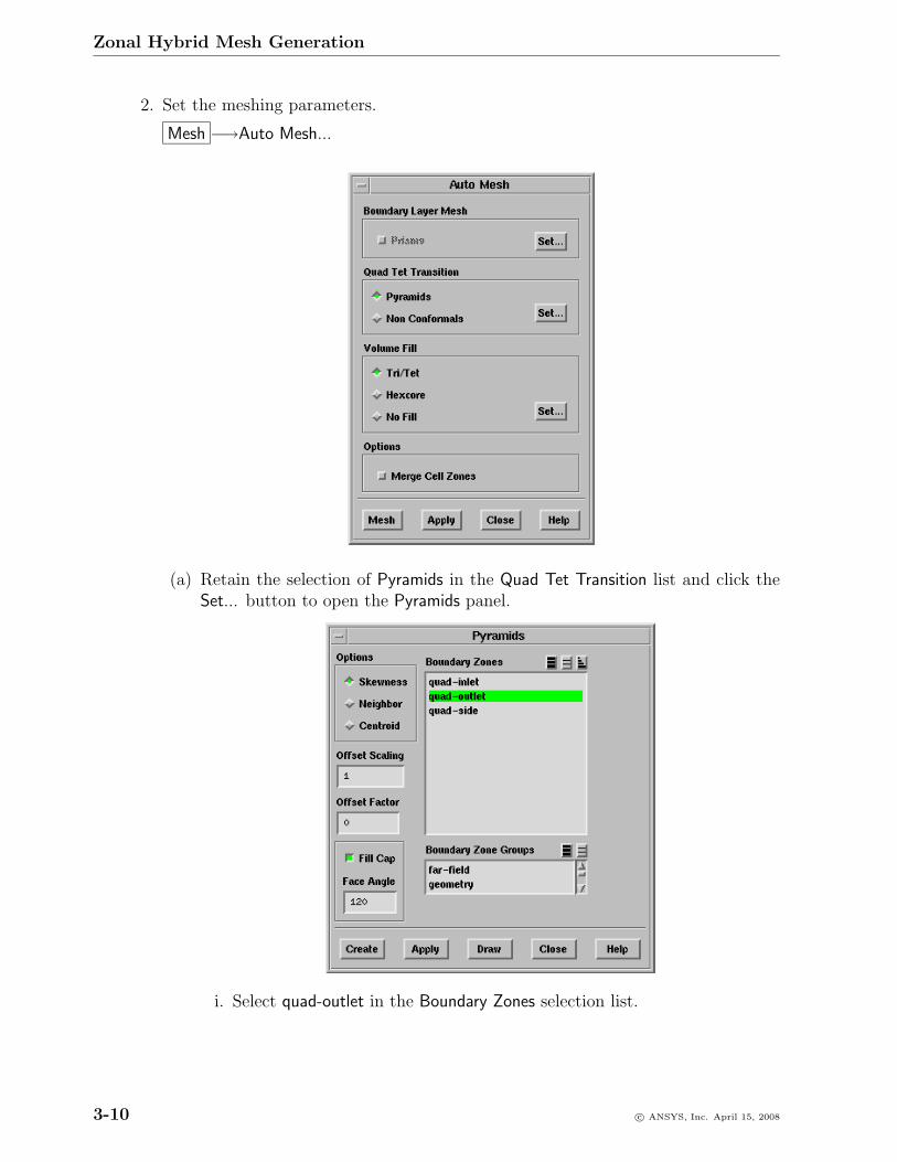
2. Set the meshing parameters.
Mesh −→Auto Mesh...
(a) Retain the selection of Pyramids in the Quad Tet Transition list and click theSet... button to open the Pyramids panel.
i. Select quad-outlet in the Boundary Zones selection list.
3-10 c© ANSYS, Inc. April 15, 2008
Zonal Hybrid Mesh Generation
ii. Retain the selection of Skewness in the Options list.
iii. Enable Fill Cap and click Apply.
iv. Close the Pyramids panel.
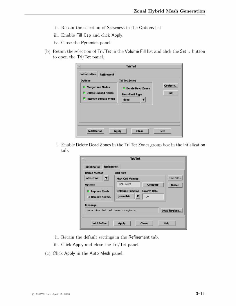
(b) Retain the selection of Tri/Tet in the Volume Fill list and click the Set... buttonto open the Tri/Tet panel.
i. Enable Delete Dead Zones in the Tri Tet Zones group box in the Intializationtab.
ii. Retain the default settings in the Refinement tab.
iii. Click Apply and close the Tri/Tet panel.
(c) Click Apply in the Auto Mesh panel.
c© ANSYS, Inc. April 15, 2008 3-11
Zonal Hybrid Mesh Generation
(d) Preserve the existing hexahedral mesh.
> /mesh/tritet/preserve-cell-zone <Enter>()Cell Zones(1) [()] fluid* <Enter>Cell Zones(2) [()] <Enter>
(e) Click Mesh in the Auto Mesh panel.
The maximum and average skewness values reported at the end of the meshingare approximately 0.816 and 0.343, respectively.
(f) Close the Auto Mesh panel.
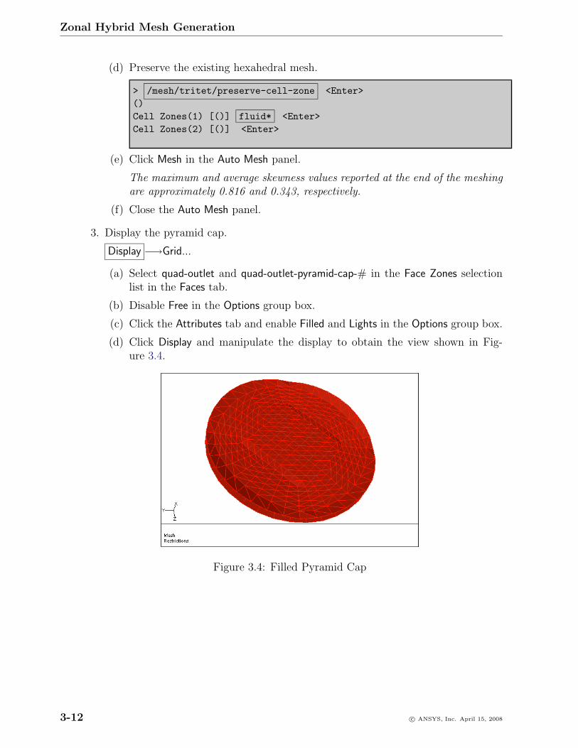
3. Display the pyramid cap.
Display −→Grid...
(a) Select quad-outlet and quad-outlet-pyramid-cap-# in the Face Zones selectionlist in the Faces tab.
(b) Disable Free in the Options group box.
(c) Click the Attributes tab and enable Filled and Lights in the Options group box.
(d) Click Display and manipulate the display to obtain the view shown in Fig-ure 3.4.
Figure 3.4: Filled Pyramid Cap
3-12 c© ANSYS, Inc. April 15, 2008
Zonal Hybrid Mesh Generation
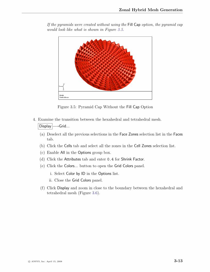
If the pyramids were created without using the Fill Cap option, the pyramid capwould look like what is shown in Figure 3.5.
Figure 3.5: Pyramid Cap Without the Fill Cap Option
4. Examine the transition between the hexahedral and tetrahedral mesh.
Display −→Grid...
(a) Deselect all the previous selections in the Face Zones selection list in the Facestab.
(b) Click the Cells tab and select all the zones in the Cell Zones selection list.
(c) Enable All in the Options group box.
(d) Click the Attributes tab and enter 0.4 for Shrink Factor.
(e) Click the Colors... button to open the Grid Colors panel.
i. Select Color by ID in the Options list.
ii. Close the Grid Colors panel.
(f) Click Display and zoom in close to the boundary between the hexahedral andtetrahedral mesh (Figure 3.6).
c© ANSYS, Inc. April 15, 2008 3-13
Zonal Hybrid Mesh Generation
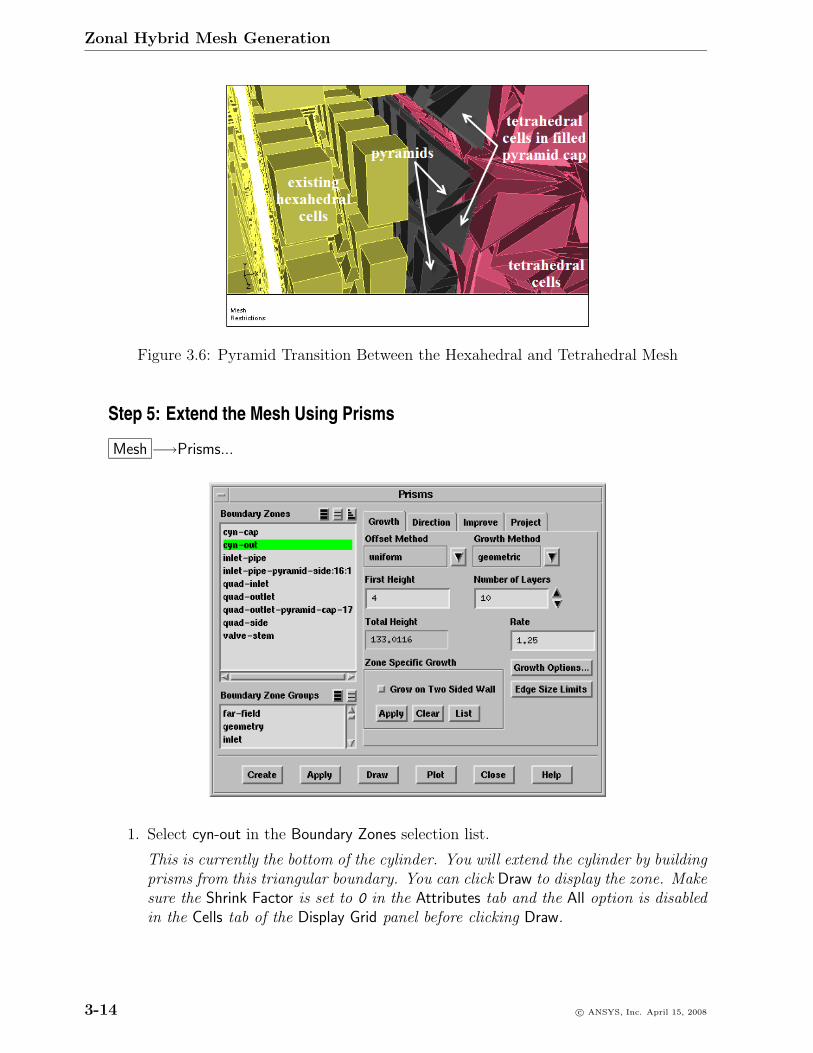
Figure 3.6: Pyramid Transition Between the Hexahedral and Tetrahedral Mesh
Step 5: Extend the Mesh Using Prisms
Mesh −→Prisms...
1. Select cyn-out in the Boundary Zones selection list.
This is currently the bottom of the cylinder. You will extend the cylinder by buildingprisms from this triangular boundary. You can click Draw to display the zone. Makesure the Shrink Factor is set to 0 in the Attributes tab and the All option is disabledin the Cells tab of the Display Grid panel before clicking Draw.
3-14 c© ANSYS, Inc. April 15, 2008
Zonal Hybrid Mesh Generation
2. Set the parameters controlling prism growth.
(a) Retain the selection of uniform in the Offset Method drop-down list and selectgeometric in the Growth Method drop-down list, respectively.
(b) Enter 4 for First Height and 1.25 for Rate, respectively.
This means that the first prism layer will have a height of 4, the second aheight of 5 (4 × 1.25), and so on.
(c) Enter 10 for Number of Layers.
The Total Height added by the prisms is slightly more than 133.
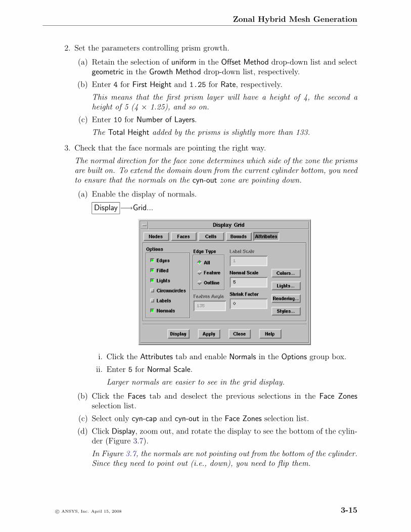
3. Check that the face normals are pointing the right way.
The normal direction for the face zone determines which side of the zone the prismsare built on. To extend the domain down from the current cylinder bottom, you needto ensure that the normals on the cyn-out zone are pointing down.
(a) Enable the display of normals.
Display −→Grid...
i. Click the Attributes tab and enable Normals in the Options group box.
ii. Enter 5 for Normal Scale.
Larger normals are easier to see in the grid display.
(b) Click the Faces tab and deselect the previous selections in the Face Zonesselection list.
(c) Select only cyn-cap and cyn-out in the Face Zones selection list.
(d) Click Display, zoom out, and rotate the display to see the bottom of the cylin-der (Figure 3.7).
In Figure 3.7, the normals are not pointing out from the bottom of the cylinder.Since they need to point out (i.e., down), you need to flip them.
c© ANSYS, Inc. April 15, 2008 3-15
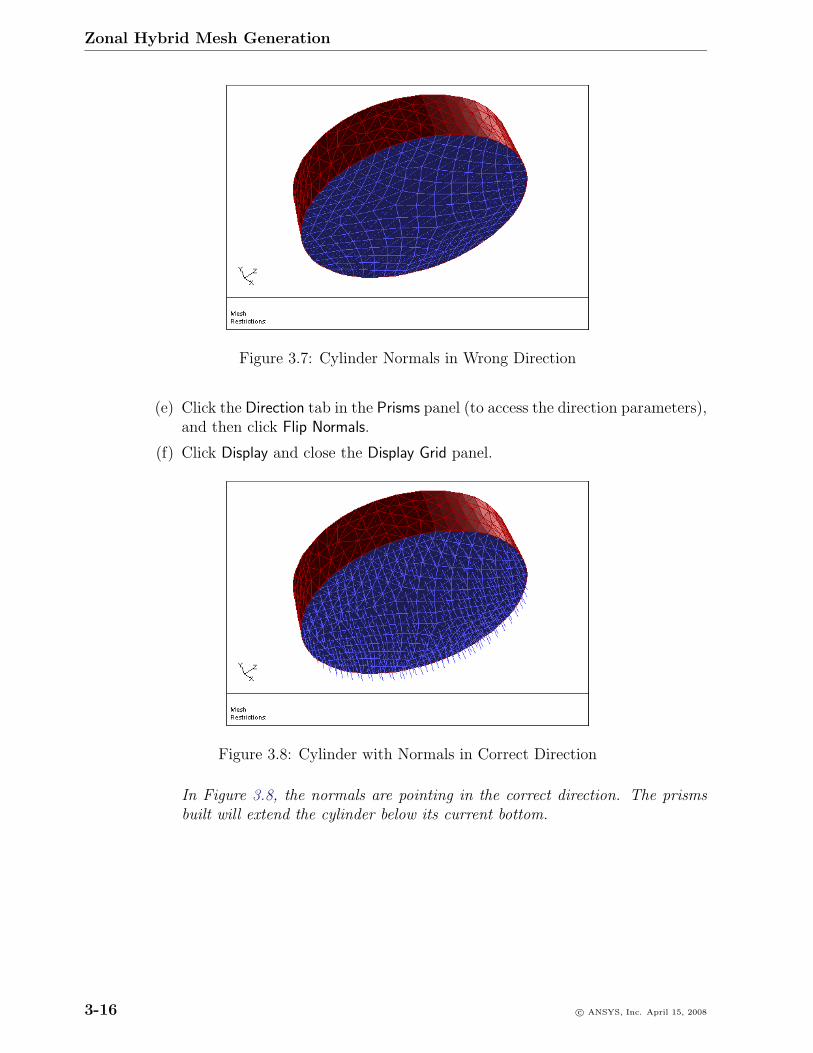
Zonal Hybrid Mesh Generation
Figure 3.7: Cylinder Normals in Wrong Direction
(e) Click the Direction tab in the Prisms panel (to access the direction parameters),and then click Flip Normals.
(f) Click Display and close the Display Grid panel.
Figure 3.8: Cylinder with Normals in Correct Direction
In Figure 3.8, the normals are pointing in the correct direction. The prismsbuilt will extend the cylinder below its current bottom.
3-16 c© ANSYS, Inc. April 15, 2008
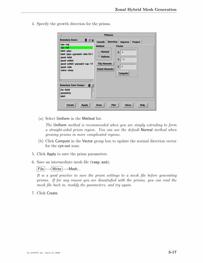
Zonal Hybrid Mesh Generation
4. Specify the growth direction for the prisms.
(a) Select Uniform in the Method list.
The Uniform method is recommended when you are simply extruding to forma straight-sided prism region. You can use the default Normal method whengrowing prisms in more complicated regions.
(b) Click Compute in the Vector group box to update the normal direction vectorfor the cyn-out zone.
5. Click Apply to save the prism parameters.
6. Save an intermediate mesh file (temp.msh).
File −→ Write −→Mesh...
It is a good practice to save the prism settings to a mesh file before generatingprisms. If for any reason you are dissatisfied with the prisms, you can read themesh file back in, modify the parameters, and try again.
7. Click Create.
c© ANSYS, Inc. April 15, 2008 3-17
Zonal Hybrid Mesh Generation
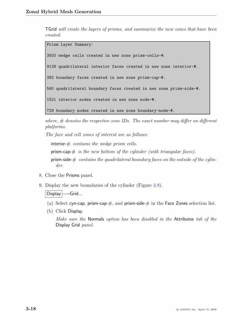
TGrid will create the layers of prisms, and summarize the new zones that have beencreated:
Prism Layer Summary:
3920 wedge cells created in new zone prism-cells-#.
9128 quadrilateral interior faces created in new zone interior-#.
392 boundary faces created in new zone prism-cap-#.
560 quadrilateral boundary faces created in new zone prism-side-#.
1521 interior nodes created in new zone node-#.
729 boundary nodes created in new zone boundary-node-#.
where, # denotes the respective zone IDs. The exact number may differ on differentplatforms.
The face and cell zones of interest are as follows:
interior-# contains the wedge prism cells.
prism-cap-# is the new bottom of the cylinder (with triangular faces).
prism-side-# contains the quadrilateral boundary faces on the outside of the cylin-der.
8. Close the Prisms panel.
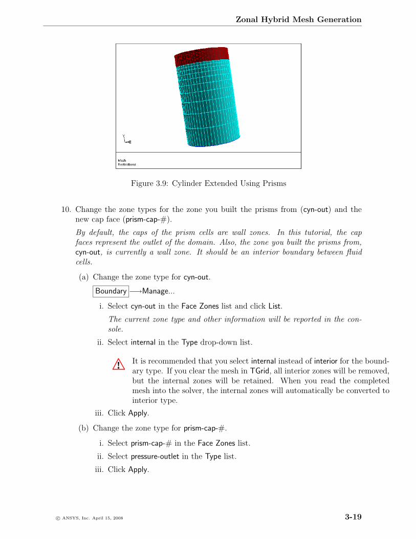
9. Display the new boundaries of the cylinder (Figure 3.9).
Display −→Grid...
(a) Select cyn-cap, prism-cap-#, and prism-side-# in the Face Zones selection list.
(b) Click Display.
Make sure the Normals option has been disabled in the Attributes tab of theDisplay Grid panel.
3-18 c© ANSYS, Inc. April 15, 2008
Zonal Hybrid Mesh Generation
Figure 3.9: Cylinder Extended Using Prisms
10. Change the zone types for the zone you built the prisms from (cyn-out) and thenew cap face (prism-cap-#).
By default, the caps of the prism cells are wall zones. In this tutorial, the capfaces represent the outlet of the domain. Also, the zone you built the prisms from,cyn-out, is currently a wall zone. It should be an interior boundary between fluidcells.
(a) Change the zone type for cyn-out.
Boundary −→Manage...
i. Select cyn-out in the Face Zones list and click List.
The current zone type and other information will be reported in the con-sole.
ii. Select internal in the Type drop-down list.
! It is recommended that you select internal instead of interior for the bound-ary type. If you clear the mesh in TGrid, all interior zones will be removed,but the internal zones will be retained. When you read the completedmesh into the solver, the internal zones will automatically be converted tointerior type.
iii. Click Apply.
(b) Change the zone type for prism-cap-#.
i. Select prism-cap-# in the Face Zones list.
ii. Select pressure-outlet in the Type list.
iii. Click Apply.
c© ANSYS, Inc. April 15, 2008 3-19
Zonal Hybrid Mesh Generation
If required, you can change the zone names using the Rename option in theManage Face Zones panel.
(c) Close the Manage Face Zones panel.
Step 6: Check and Save the Volume Mesh
1. Check the skewness of the entire volume mesh.
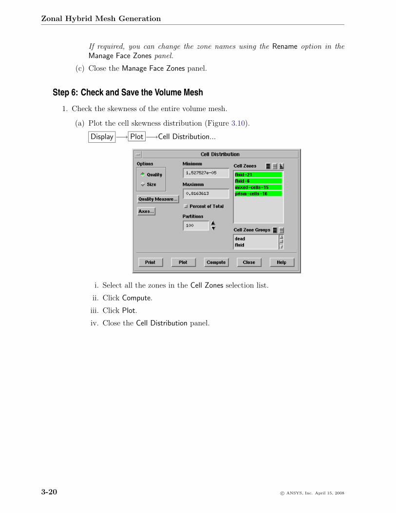
(a) Plot the cell skewness distribution (Figure 3.10).
Display −→ Plot −→Cell Distribution...
i. Select all the zones in the Cell Zones selection list.
ii. Click Compute.
iii. Click Plot.
iv. Close the Cell Distribution panel.
3-20 c© ANSYS, Inc. April 15, 2008
Zonal Hybrid Mesh Generation
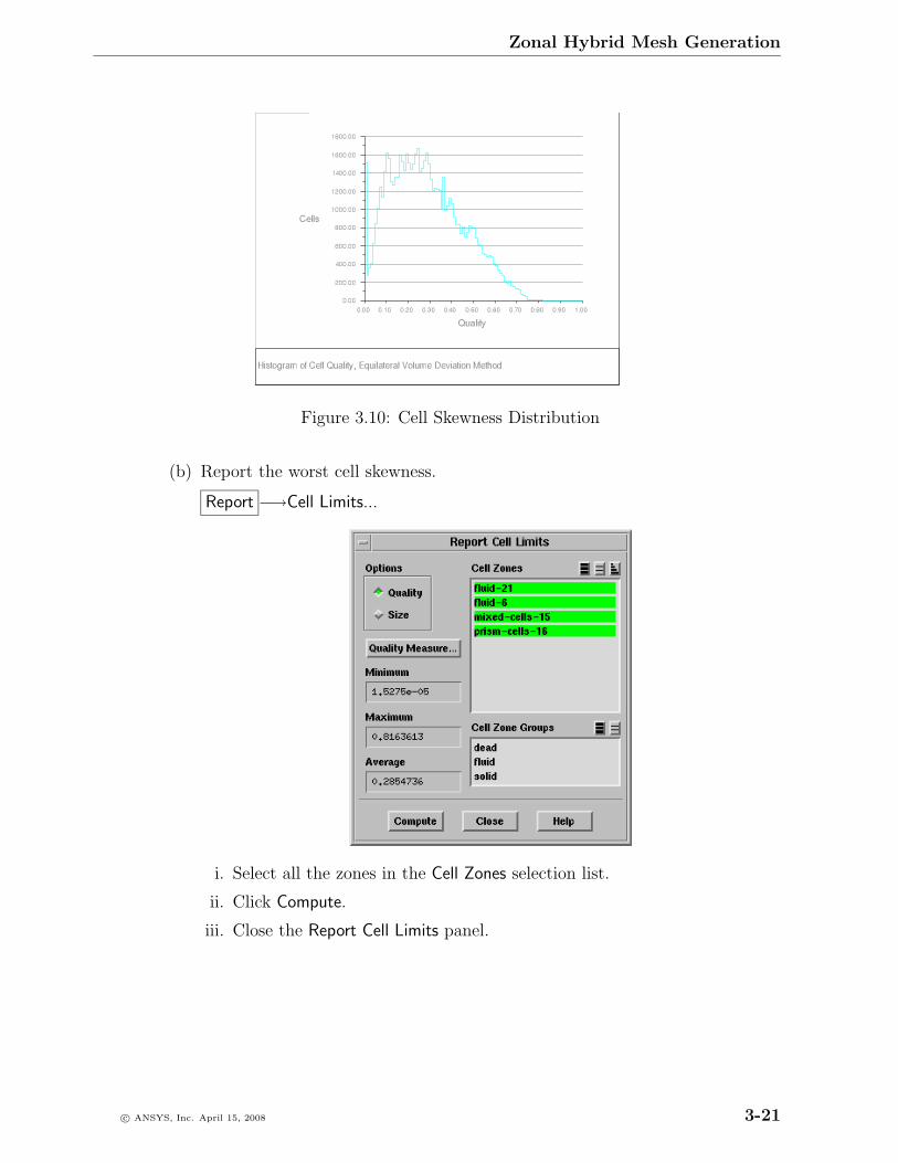
Figure 3.10: Cell Skewness Distribution
(b) Report the worst cell skewness.
Report −→Cell Limits...
i. Select all the zones in the Cell Zones selection list.
ii. Click Compute.
iii. Close the Report Cell Limits panel.
c© ANSYS, Inc. April 15, 2008 3-21
Zonal Hybrid Mesh Generation
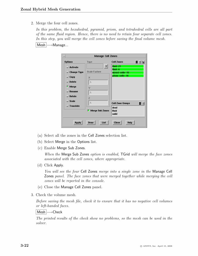
2. Merge the four cell zones.
In this problem, the hexahedral, pyramid, prism, and tetrahedral cells are all partof the same fluid region. Hence, there is no need to retain four separate cell zones.In this step, you will merge the cell zones before saving the final volume mesh.
Mesh −→Manage...
(a) Select all the zones in the Cell Zones selection list.
(b) Select Merge in the Options list.
(c) Enable Merge Sub Zones.
When the Merge Sub Zones option is enabled, TGrid will merge the face zonesassociated with the cell zones, where appropriate.
(d) Click Apply.
You will see the four Cell Zones merge into a single zone in the Manage CellZones panel. The face zones that were merged together while merging the cellzones will be reported in the console.
(e) Close the Manage Cell Zones panel.
3. Check the volume mesh.
Before saving the mesh file, check it to ensure that it has no negative cell volumesor left-handed faces.
Mesh −→Check
The printed results of the check show no problems, so the mesh can be used in thesolver.
3-22 c© ANSYS, Inc. April 15, 2008
Zonal Hybrid Mesh Generation
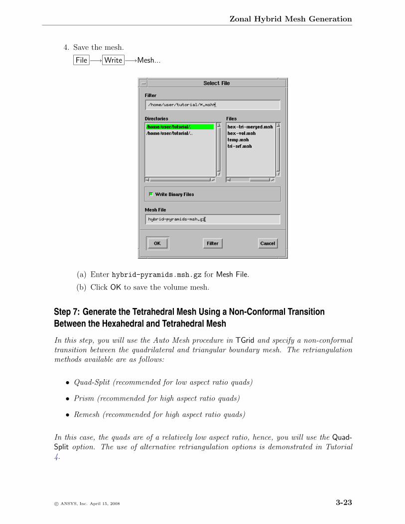
4. Save the mesh.
File −→ Write −→Mesh...
(a) Enter hybrid-pyramids.msh.gz for Mesh File.
(b) Click OK to save the volume mesh.
Step 7: Generate the Tetrahedral Mesh Using a Non-Conformal TransitionBetween the Hexahedral and Tetrahedral Mesh
In this step, you will use the Auto Mesh procedure in TGrid and specify a non-conformaltransition between the quadrilateral and triangular boundary mesh. The retriangulationmethods available are as follows:
• Quad-Split (recommended for low aspect ratio quads)
• Prism (recommended for high aspect ratio quads)
• Remesh (recommended for high aspect ratio quads)
In this case, the quads are of a relatively low aspect ratio, hence, you will use the Quad-Split option. The use of alternative retriangulation options is demonstrated in Tutorial4.
c© ANSYS, Inc. April 15, 2008 3-23
Zonal Hybrid Mesh Generation
Note: The steps in this section are similar to those described in previous sections, andhence are less explicit.
1. Read the mesh file saved after merging the free nodes (hex-tri-merged.msh).
File −→ Read −→Mesh...
2. Change the type of the quad-outlet zone to internal.
Boundary −→Manage...
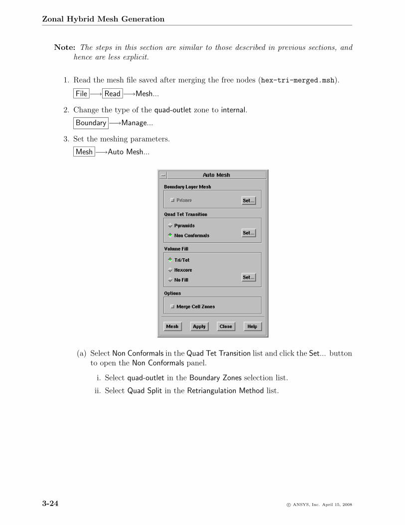
3. Set the meshing parameters.
Mesh −→Auto Mesh...
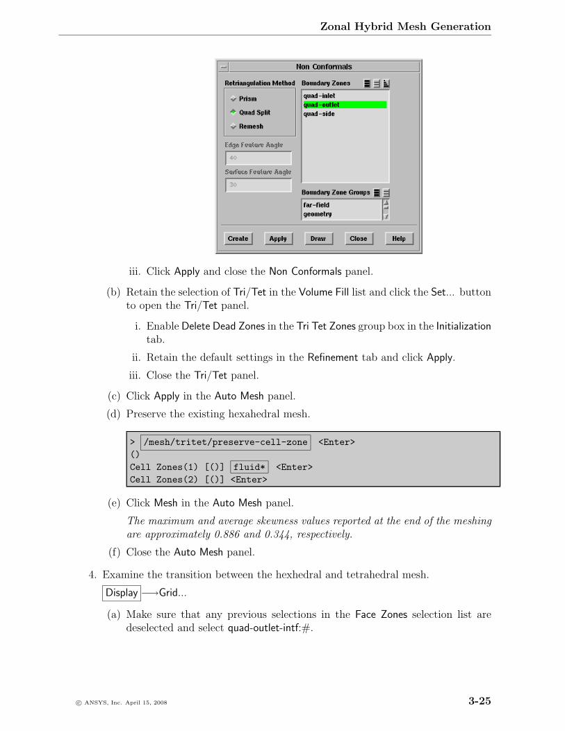
(a) Select Non Conformals in the Quad Tet Transition list and click the Set... buttonto open the Non Conformals panel.
i. Select quad-outlet in the Boundary Zones selection list.
ii. Select Quad Split in the Retriangulation Method list.
3-24 c© ANSYS, Inc. April 15, 2008
Zonal Hybrid Mesh Generation
iii. Click Apply and close the Non Conformals panel.
(b) Retain the selection of Tri/Tet in the Volume Fill list and click the Set... buttonto open the Tri/Tet panel.
i. Enable Delete Dead Zones in the Tri Tet Zones group box in the Initializationtab.
ii. Retain the default settings in the Refinement tab and click Apply.
iii. Close the Tri/Tet panel.
(c) Click Apply in the Auto Mesh panel.
(d) Preserve the existing hexahedral mesh.
> /mesh/tritet/preserve-cell-zone <Enter>()Cell Zones(1) [()] fluid* <Enter>Cell Zones(2) [()] <Enter>
(e) Click Mesh in the Auto Mesh panel.
The maximum and average skewness values reported at the end of the meshingare approximately 0.886 and 0.344, respectively.
(f) Close the Auto Mesh panel.
4. Examine the transition between the hexhedral and tetrahedral mesh.
Display −→Grid...
(a) Make sure that any previous selections in the Face Zones selection list aredeselected and select quad-outlet-intf:#.
c© ANSYS, Inc. April 15, 2008 3-25
Zonal Hybrid Mesh Generation
(b) Disable Free in the Options group box in the Faces tab.
(c) Click the Cells tab and select all the zones in the Cell Zones selection list.
(d) Enable All in the Options group box.
(e) Click the Attributes tab and enable Filled and Lights in the Options group box.
(f) Enter 0.4 for Shrink Factor.
(g) Click the Colors... button to open the Grid Colors panel.
i. Select Color by ID in the Options list.
ii. Close the Grid Colors panel.
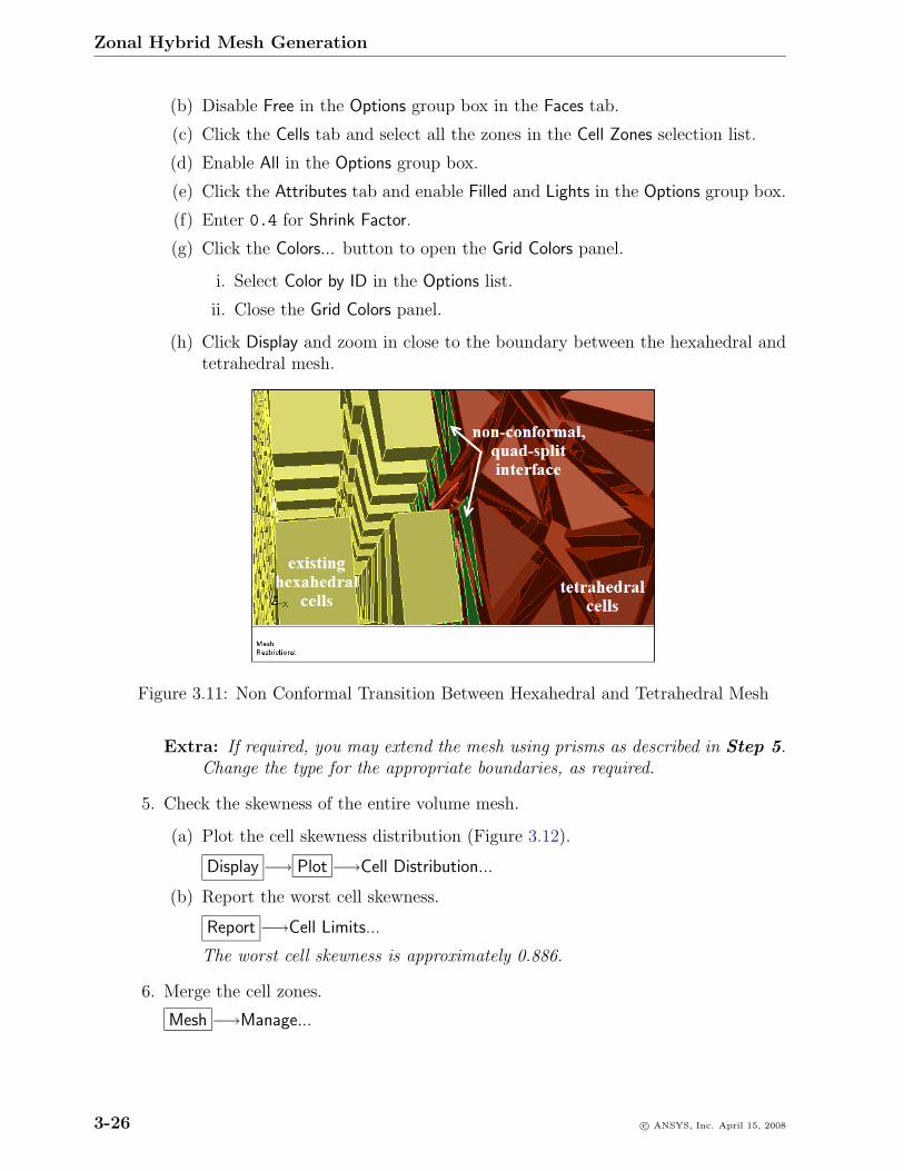
(h) Click Display and zoom in close to the boundary between the hexahedral andtetrahedral mesh.
Figure 3.11: Non Conformal Transition Between Hexahedral and Tetrahedral Mesh
Extra: If required, you may extend the mesh using prisms as described in Step 5.Change the type for the appropriate boundaries, as required.
5. Check the skewness of the entire volume mesh.
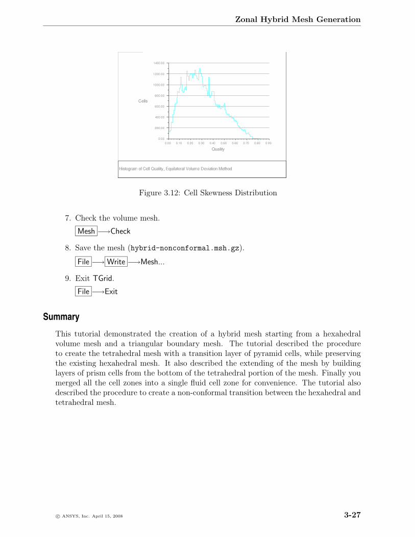
(a) Plot the cell skewness distribution (Figure 3.12).
Display −→ Plot −→Cell Distribution...
(b) Report the worst cell skewness.
Report −→Cell Limits...
The worst cell skewness is approximately 0.886.
6. Merge the cell zones.
Mesh −→Manage...
3-26 c© ANSYS, Inc. April 15, 2008
Zonal Hybrid Mesh Generation
Figure 3.12: Cell Skewness Distribution
7. Check the volume mesh.
Mesh −→Check
8. Save the mesh (hybrid-nonconformal.msh.gz).
File −→ Write −→Mesh...
9. Exit TGrid.
File −→Exit
Summary
This tutorial demonstrated the creation of a hybrid mesh starting from a hexahedralvolume mesh and a triangular boundary mesh. The tutorial described the procedureto create the tetrahedral mesh with a transition layer of pyramid cells, while preservingthe existing hexahedral mesh. It also described the extending of the mesh by buildinglayers of prism cells from the bottom of the tetrahedral portion of the mesh. Finally youmerged all the cell zones into a single fluid cell zone for convenience. The tutorial alsodescribed the procedure to create a non-conformal transition between the hexahedral andtetrahedral mesh.
c© ANSYS, Inc. April 15, 2008 3-27

Zonal Hybrid Mesh Generation
3-28 c© ANSYS, Inc. April 15, 2008
Tutorial 4. Viscous Hybrid Mesh Generation
Introduction
In cases where you want to resolve the boundary layer, it is often more efficient to useprismatic cells in the boundary layer rather than tetrahedral cells. The prismatic cellsallow you to resolve the normal gradients associated with boundary layers with fewercells. The resulting mesh is referred to as a “viscous” hybrid mesh.
TGrid allows you to create a viscous hybrid mesh by growing prisms from the faces on thesurface mesh. It creates high quality prism elements near the boundary and tetrahedralelements in the rest of the domain. TGrid also supports automatic proximity detectionand height adjustment while growing prisms in a narrow gap.
This tutorial demonstrates the mesh generation procedure for a viscous hybrid mesh,starting from a triangular boundary mesh for a sedan car body. This tutorial demon-strates how to do the following:
1. Read the mesh file and display the boundary mesh.
2. Check for free and unused nodes.
3. Check the skewness of the boundary faces.
4. Set parameters for growing prism cells allowing shrinkage and manual tetrahedralmeshing.
5. Set parameters for growing prism cells ignoring areas of proximity and automaticmeshing.
6. Examine the prisms in areas of proximity and sharp angles.
7. Check the skewness of the entire volume mesh.
8. Check and save the volume mesh.
Prerequisites
This tutorial assumes that you have some experience with TGrid, and that you are familiarwith the graphical user interface.
c© ANSYS, Inc. April 15, 2008 4-1
Viscous Hybrid Mesh Generation
Preparation
1. Download prisms.zip from the FLUENT User Services Center to your workingdirectory. This file can be found from the Documentation link on the TGrid productpage.
OR
Copy prisms.zip from the TGrid documentation CD to your working directory.
• For UNIX systems, insert the CD into your CD-ROM drive and go to thefollowing directory:
cdrom/tgrid5.0/help/tutfiles
where, cdrom must be replaced by the name of your CD-ROM drive.
• For Windows systems, insert the CD into your CD-ROM drive and go to thefollowing folder:
cdrom:\tgrid5.0\help\tutfiles
where, cdrom must be replaced by the name of your CD-ROM drive (e.g., E).
2. Unzip prisms.zip.
The file, sedan.msh.gz can be found in the prisms folder created on unzipping thefile.
3. Start the 3D (3d) version of TGrid.
4-2 c© ANSYS, Inc. April 15, 2008

Viscous Hybrid Mesh Generation
Step 1: Read and Display the Boundary Mesh
1. Read the mesh file.
File −→ Read −→Boundary Mesh...
(a) Select sedan.msh.gz in the Files list.
(b) Click OK.
c© ANSYS, Inc. April 15, 2008 4-3
Viscous Hybrid Mesh Generation
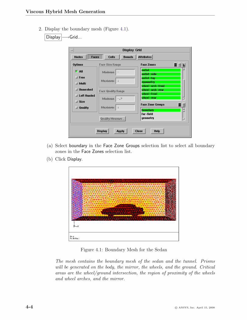
2. Display the boundary mesh (Figure 4.1).
Display −→Grid...
(a) Select boundary in the Face Zone Groups selection list to select all boundaryzones in the Face Zones selection list.
(b) Click Display.
Figure 4.1: Boundary Mesh for the Sedan
The mesh contains the boundary mesh of the sedan and the tunnel. Prismswill be generated on the body, the mirror, the wheels, and the ground. Criticalareas are the wheel/ground intersection, the region of proximity of the wheelsand wheel arches, and the mirror.
4-4 c© ANSYS, Inc. April 15, 2008
Viscous Hybrid Mesh Generation
(c) Close the Display Grid panel.
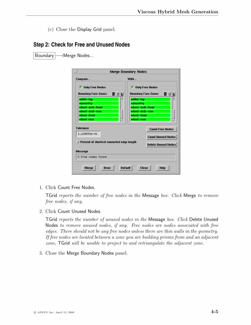
Step 2: Check for Free and Unused Nodes
Boundary −→Merge Nodes...
1. Click Count Free Nodes.
TGrid reports the number of free nodes in the Message box. Click Merge to removefree nodes, if any.
2. Click Count Unused Nodes.
TGrid reports the number of unused nodes in the Message box. Click Delete UnusedNodes to remove unused nodes, if any. Free nodes are nodes associated with freeedges. There should not be any free nodes unless there are thin walls in the geometry.If free nodes are located between a zone you are building prisms from and an adjacentzone, TGrid will be unable to project to and retriangulate the adjacent zone.
3. Close the Merge Boundary Nodes panel.
c© ANSYS, Inc. April 15, 2008 4-5
Viscous Hybrid Mesh Generation
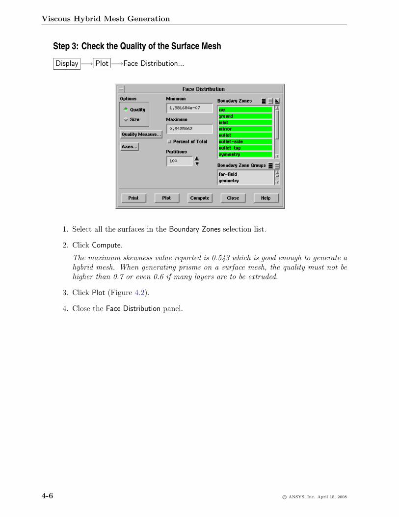
Step 3: Check the Quality of the Surface Mesh
Display −→ Plot −→Face Distribution...
1. Select all the surfaces in the Boundary Zones selection list.
2. Click Compute.
The maximum skewness value reported is 0.543 which is good enough to generate ahybrid mesh. When generating prisms on a surface mesh, the quality must not behigher than 0.7 or even 0.6 if many layers are to be extruded.
3. Click Plot (Figure 4.2).
4. Close the Face Distribution panel.
4-6 c© ANSYS, Inc. April 15, 2008
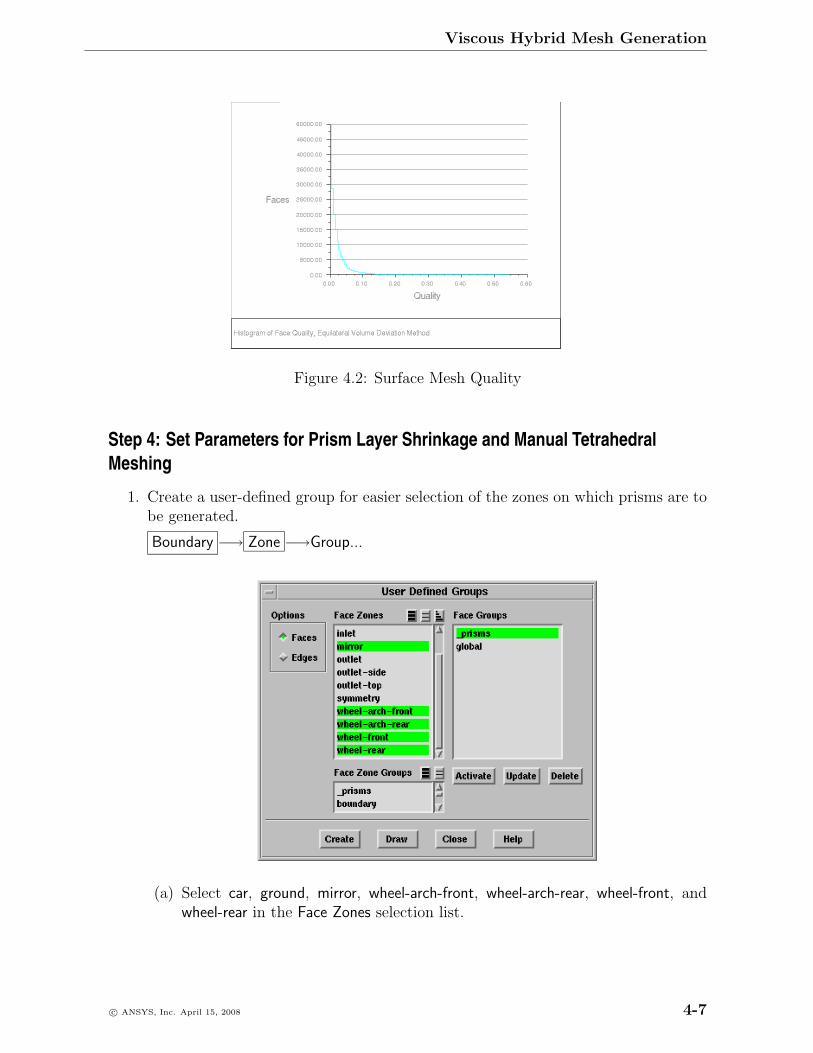
Viscous Hybrid Mesh Generation
Figure 4.2: Surface Mesh Quality
Step 4: Set Parameters for Prism Layer Shrinkage and Manual TetrahedralMeshing
1. Create a user-defined group for easier selection of the zones on which prisms are tobe generated.
Boundary −→ Zone −→Group...
(a) Select car, ground, mirror, wheel-arch-front, wheel-arch-rear, wheel-front, andwheel-rear in the Face Zones selection list.
c© ANSYS, Inc. April 15, 2008 4-7
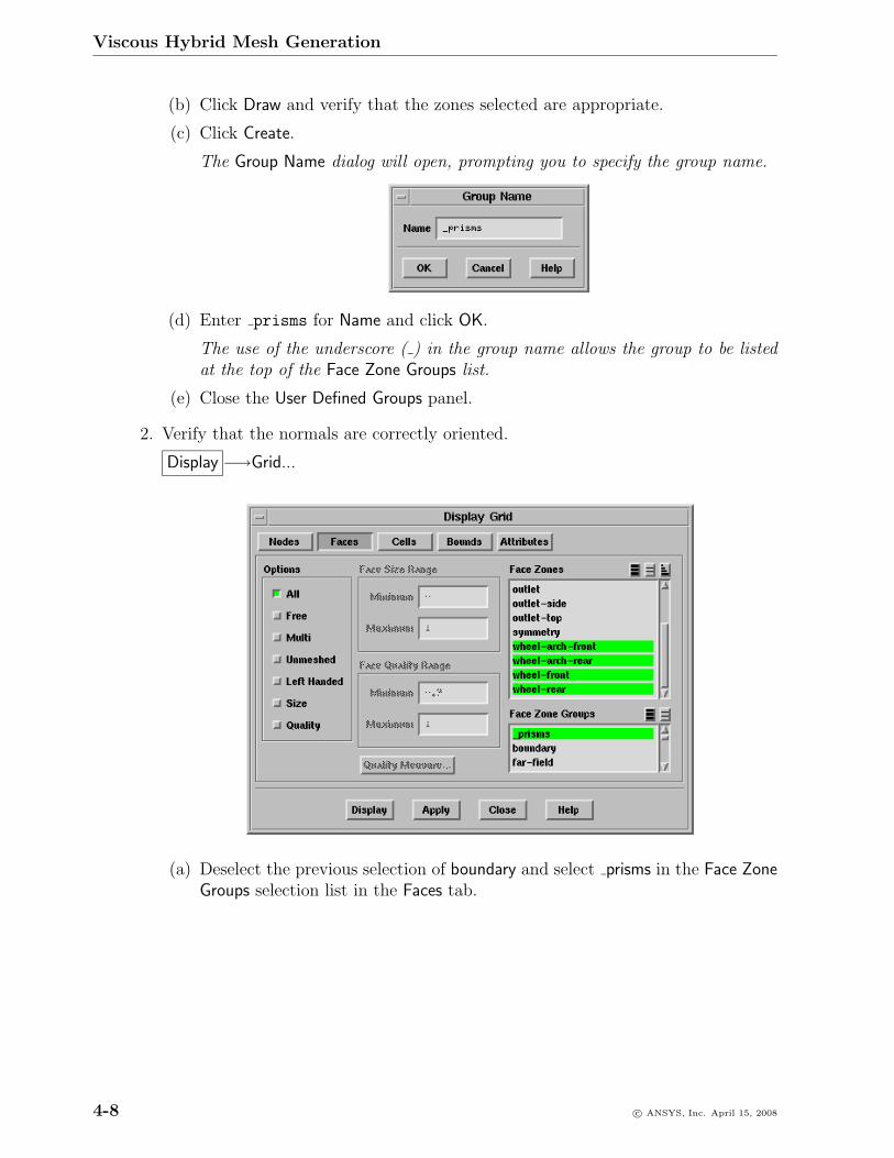
Viscous Hybrid Mesh Generation
(b) Click Draw and verify that the zones selected are appropriate.
(c) Click Create.
The Group Name dialog will open, prompting you to specify the group name.
(d) Enter prisms for Name and click OK.
The use of the underscore ( ) in the group name allows the group to be listedat the top of the Face Zone Groups list.
(e) Close the User Defined Groups panel.
2. Verify that the normals are correctly oriented.
Display −→Grid...
(a) Deselect the previous selection of boundary and select prisms in the Face ZoneGroups selection list in the Faces tab.
4-8 c© ANSYS, Inc. April 15, 2008
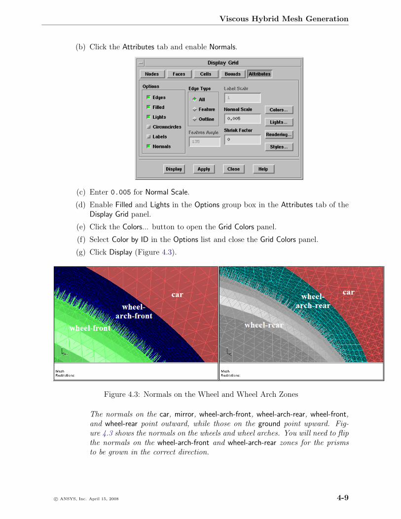
Viscous Hybrid Mesh Generation
(b) Click the Attributes tab and enable Normals.
(c) Enter 0.005 for Normal Scale.
(d) Enable Filled and Lights in the Options group box in the Attributes tab of theDisplay Grid panel.
(e) Click the Colors... button to open the Grid Colors panel.
(f) Select Color by ID in the Options list and close the Grid Colors panel.
(g) Click Display (Figure 4.3).
Figure 4.3: Normals on the Wheel and Wheel Arch Zones
The normals on the car, mirror, wheel-arch-front, wheel-arch-rear, wheel-front,and wheel-rear point outward, while those on the ground point upward. Fig-ure 4.3 shows the normals on the wheels and wheel arches. You will need to flipthe normals on the wheel-arch-front and wheel-arch-rear zones for the prismsto be grown in the correct direction.
c© ANSYS, Inc. April 15, 2008 4-9
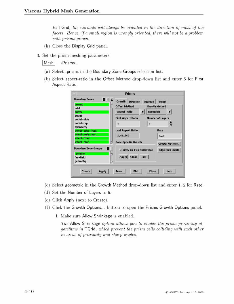
Viscous Hybrid Mesh Generation
In TGrid, the normals will always be oriented in the direction of most of thefacets. Hence, if a small region is wrongly oriented, there will not be a problemwith prisms grown.
(h) Close the Display Grid panel.
3. Set the prism meshing parameters.
Mesh −→Prisms...
(a) Select prisms in the Boundary Zone Groups selection list.
(b) Select aspect-ratio in the Offset Method drop-down list and enter 5 for FirstAspect Ratio.
(c) Select geometric in the Growth Method drop-down list and enter 1.2 for Rate.
(d) Set the Number of Layers to 5.
(e) Click Apply (next to Create).
(f) Click the Growth Options... button to open the Prisms Growth Options panel.
i. Make sure Allow Shrinkage is enabled.
The Allow Shrinkage option allows you to enable the prism proximity al-gorithms in TGrid, which prevent the prism cells colliding with each otherin areas of proximity and sharp angles.
4-10 c© ANSYS, Inc. April 15, 2008
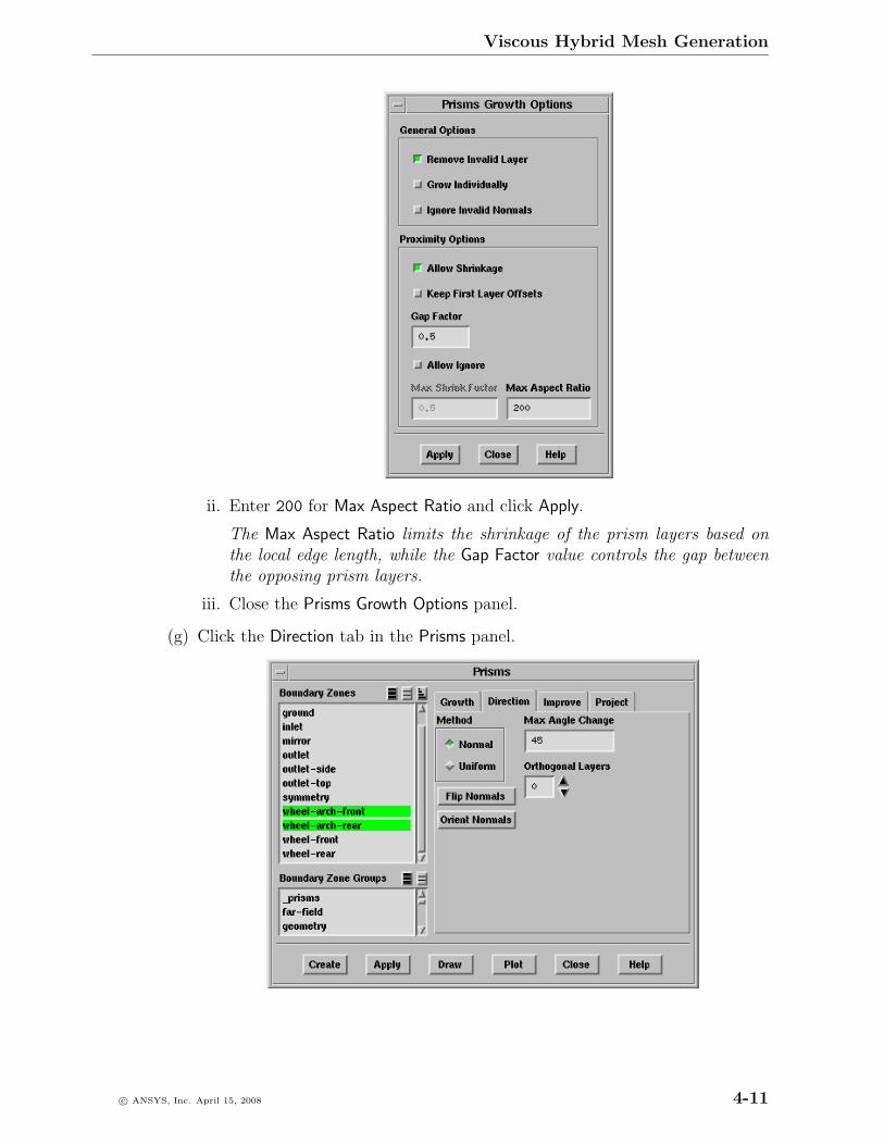
Viscous Hybrid Mesh Generation
ii. Enter 200 for Max Aspect Ratio and click Apply.
The Max Aspect Ratio limits the shrinkage of the prism layers based onthe local edge length, while the Gap Factor value controls the gap betweenthe opposing prism layers.
iii. Close the Prisms Growth Options panel.
(g) Click the Direction tab in the Prisms panel.
c© ANSYS, Inc. April 15, 2008 4-11
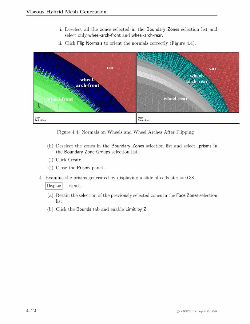
Viscous Hybrid Mesh Generation
i. Deselect all the zones selected in the Boundary Zones selection list andselect only wheel-arch-front and wheel-arch-rear.
ii. Click Flip Normals to orient the normals correctly (Figure 4.4).
Figure 4.4: Normals on Wheels and Wheel Arches After Flipping
(h) Deselect the zones in the Boundary Zones selection list and select prisms inthe Boundary Zone Groups selection list.
(i) Click Create.
(j) Close the Prisms panel.
4. Examine the prisms generated by displaying a slide of cells at z = 0.38.
Display −→Grid...
(a) Retain the selection of the previously selected zones in the Face Zones selectionlist.
(b) Click the Bounds tab and enable Limit by Z.
4-12 c© ANSYS, Inc. April 15, 2008
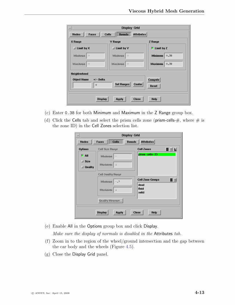
Viscous Hybrid Mesh Generation
(c) Enter 0.38 for both Minimum and Maximum in the Z Range group box.
(d) Click the Cells tab and select the prism cells zone (prism-cells-#, where # isthe zone ID) in the Cell Zones selection list.
(e) Enable All in the Options group box and click Display.
Make sure the display of normals is disabled in the Attributes tab.
(f) Zoom in to the region of the wheel/ground intersection and the gap betweenthe car body and the wheels (Figure 4.5).
(g) Close the Display Grid panel.
c© ANSYS, Inc. April 15, 2008 4-13
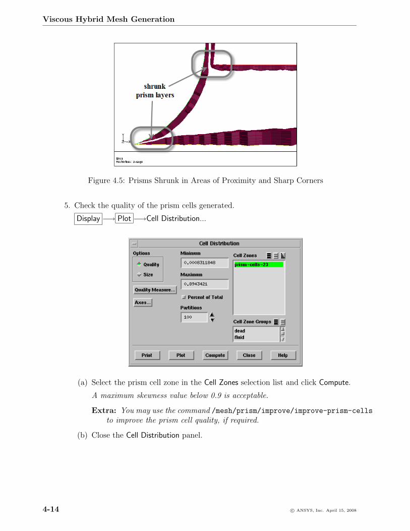
Viscous Hybrid Mesh Generation
Figure 4.5: Prisms Shrunk in Areas of Proximity and Sharp Corners
5. Check the quality of the prism cells generated.
Display −→ Plot −→Cell Distribution...
(a) Select the prism cell zone in the Cell Zones selection list and click Compute.
A maximum skewness value below 0.9 is acceptable.
Extra: You may use the command /mesh/prism/improve/improve-prism-cells
to improve the prism cell quality, if required.
(b) Close the Cell Distribution panel.
4-14 c© ANSYS, Inc. April 15, 2008
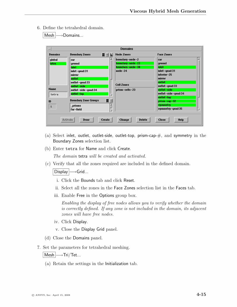
Viscous Hybrid Mesh Generation
6. Define the tetrahedral domain.
Mesh −→Domains...
(a) Select inlet, outlet, outlet-side, outlet-top, prism-cap-#, and symmetry in theBoundary Zones selection list.
(b) Enter tetra for Name and click Create.
The domain tetra will be created and activated.
(c) Verify that all the zones required are included in the defined domain.
Display −→Grid...
i. Click the Bounds tab and click Reset.
ii. Select all the zones in the Face Zones selection list in the Faces tab.
iii. Enable Free in the Options group box.
Enabling the display of free nodes allows you to verify whether the domainis correctly defined. If any zone is not included in the domain, its adjacentzones will have free nodes.
iv. Click Display.
v. Close the Display Grid panel.
(d) Close the Domains panel.
7. Set the parameters for tetrahedral meshing.
Mesh −→Tri/Tet...
(a) Retain the settings in the Initialization tab.
c© ANSYS, Inc. April 15, 2008 4-15
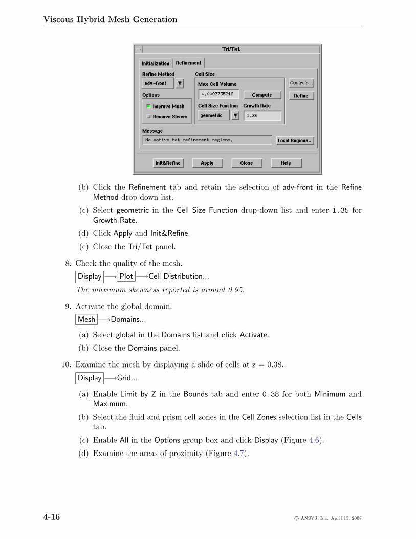
Viscous Hybrid Mesh Generation
(b) Click the Refinement tab and retain the selection of adv-front in the RefineMethod drop-down list.
(c) Select geometric in the Cell Size Function drop-down list and enter 1.35 forGrowth Rate.
(d) Click Apply and Init&Refine.
(e) Close the Tri/Tet panel.
8. Check the quality of the mesh.
Display −→ Plot −→Cell Distribution...
The maximum skewness reported is around 0.95.
9. Activate the global domain.
Mesh −→Domains...
(a) Select global in the Domains list and click Activate.
(b) Close the Domains panel.
10. Examine the mesh by displaying a slide of cells at z = 0.38.
Display −→Grid...
(a) Enable Limit by Z in the Bounds tab and enter 0.38 for both Minimum andMaximum.
(b) Select the fluid and prism cell zones in the Cell Zones selection list in the Cellstab.
(c) Enable All in the Options group box and click Display (Figure 4.6).
(d) Examine the areas of proximity (Figure 4.7).
4-16 c© ANSYS, Inc. April 15, 2008
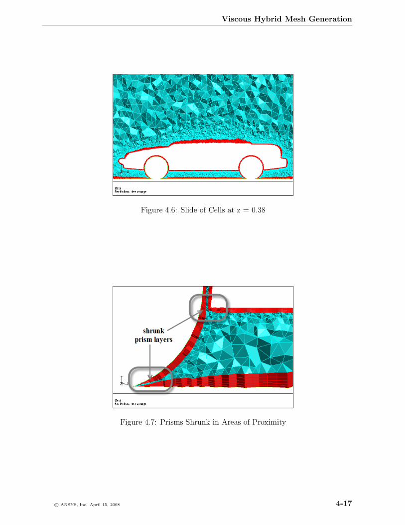
Viscous Hybrid Mesh Generation
Figure 4.6: Slide of Cells at z = 0.38
Figure 4.7: Prisms Shrunk in Areas of Proximity
c© ANSYS, Inc. April 15, 2008 4-17
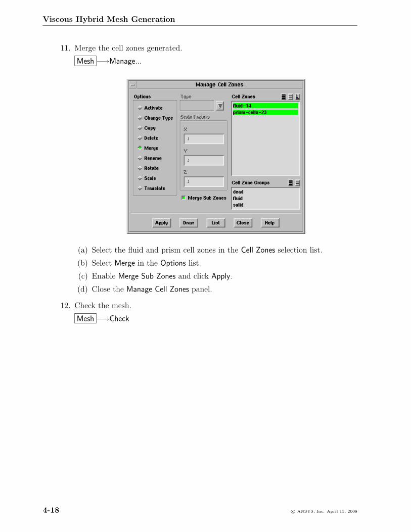
Viscous Hybrid Mesh Generation
11. Merge the cell zones generated.
Mesh −→Manage...
(a) Select the fluid and prism cell zones in the Cell Zones selection list.
(b) Select Merge in the Options list.
(c) Enable Merge Sub Zones and click Apply.
(d) Close the Manage Cell Zones panel.
12. Check the mesh.
Mesh −→Check
4-18 c© ANSYS, Inc. April 15, 2008
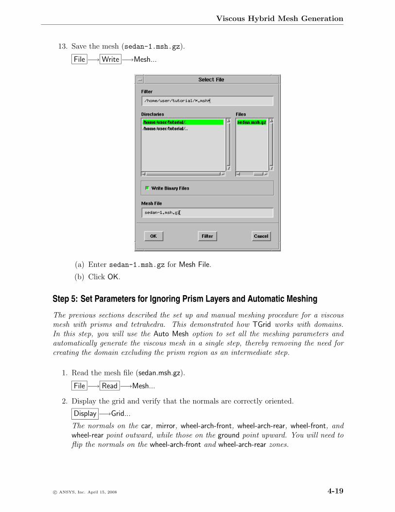
Viscous Hybrid Mesh Generation
13. Save the mesh (sedan-1.msh.gz).
File −→ Write −→Mesh...
(a) Enter sedan-1.msh.gz for Mesh File.
(b) Click OK.
Step 5: Set Parameters for Ignoring Prism Layers and Automatic Meshing
The previous sections described the set up and manual meshing procedure for a viscousmesh with prisms and tetrahedra. This demonstrated how TGrid works with domains.In this step, you will use the Auto Mesh option to set all the meshing parameters andautomatically generate the viscous mesh in a single step, thereby removing the need forcreating the domain excluding the prism region as an intermediate step.
1. Read the mesh file (sedan.msh.gz).
File −→ Read −→Mesh...
2. Display the grid and verify that the normals are correctly oriented.
Display −→Grid...
The normals on the car, mirror, wheel-arch-front, wheel-arch-rear, wheel-front, andwheel-rear point outward, while those on the ground point upward. You will need toflip the normals on the wheel-arch-front and wheel-arch-rear zones.
c© ANSYS, Inc. April 15, 2008 4-19
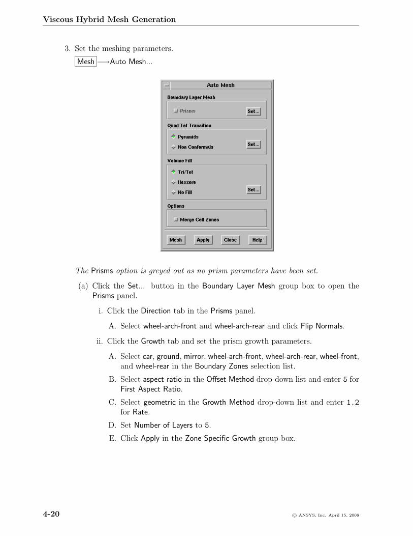
Viscous Hybrid Mesh Generation
3. Set the meshing parameters.
Mesh −→Auto Mesh...
The Prisms option is greyed out as no prism parameters have been set.
(a) Click the Set... button in the Boundary Layer Mesh group box to open thePrisms panel.
i. Click the Direction tab in the Prisms panel.
A. Select wheel-arch-front and wheel-arch-rear and click Flip Normals.
ii. Click the Growth tab and set the prism growth parameters.
A. Select car, ground, mirror, wheel-arch-front, wheel-arch-rear, wheel-front,and wheel-rear in the Boundary Zones selection list.
B. Select aspect-ratio in the Offset Method drop-down list and enter 5 forFirst Aspect Ratio.
C. Select geometric in the Growth Method drop-down list and enter 1.2
for Rate.
D. Set Number of Layers to 5.
E. Click Apply in the Zone Specific Growth group box.
4-20 c© ANSYS, Inc. April 15, 2008
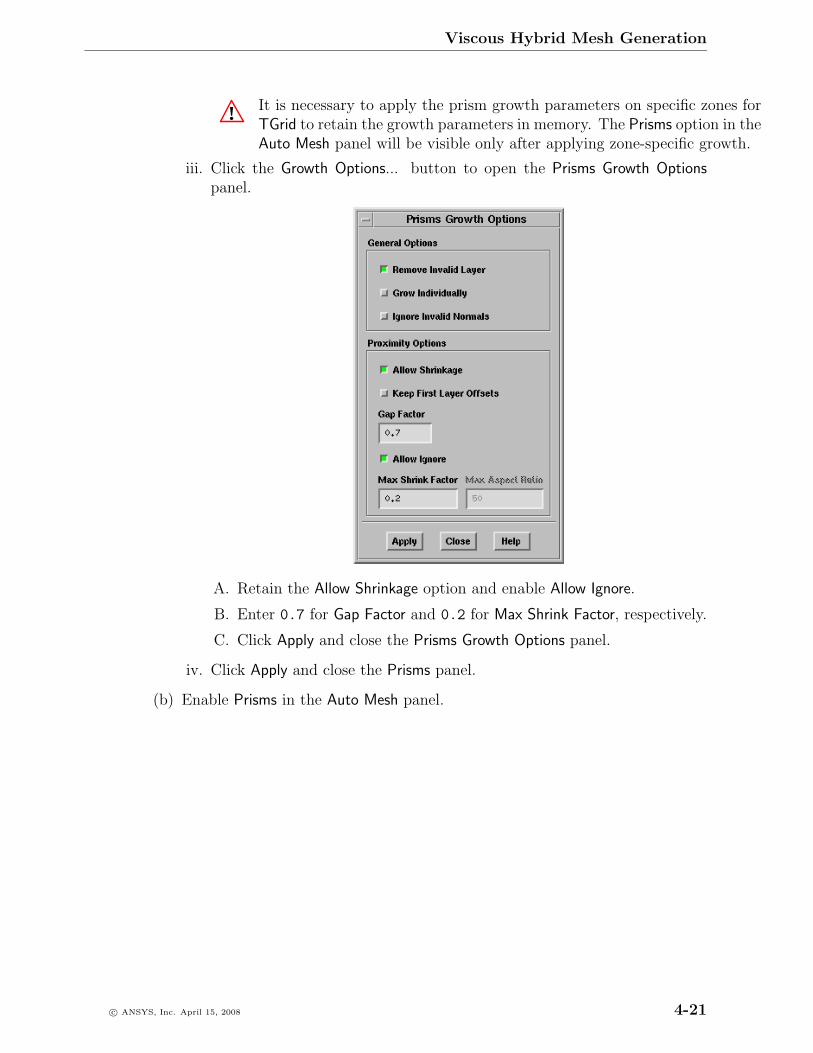
Viscous Hybrid Mesh Generation
! It is necessary to apply the prism growth parameters on specific zones forTGrid to retain the growth parameters in memory. The Prisms option in theAuto Mesh panel will be visible only after applying zone-specific growth.
iii. Click the Growth Options... button to open the Prisms Growth Optionspanel.
A. Retain the Allow Shrinkage option and enable Allow Ignore.
B. Enter 0.7 for Gap Factor and 0.2 for Max Shrink Factor, respectively.
C. Click Apply and close the Prisms Growth Options panel.
iv. Click Apply and close the Prisms panel.
(b) Enable Prisms in the Auto Mesh panel.
c© ANSYS, Inc. April 15, 2008 4-21
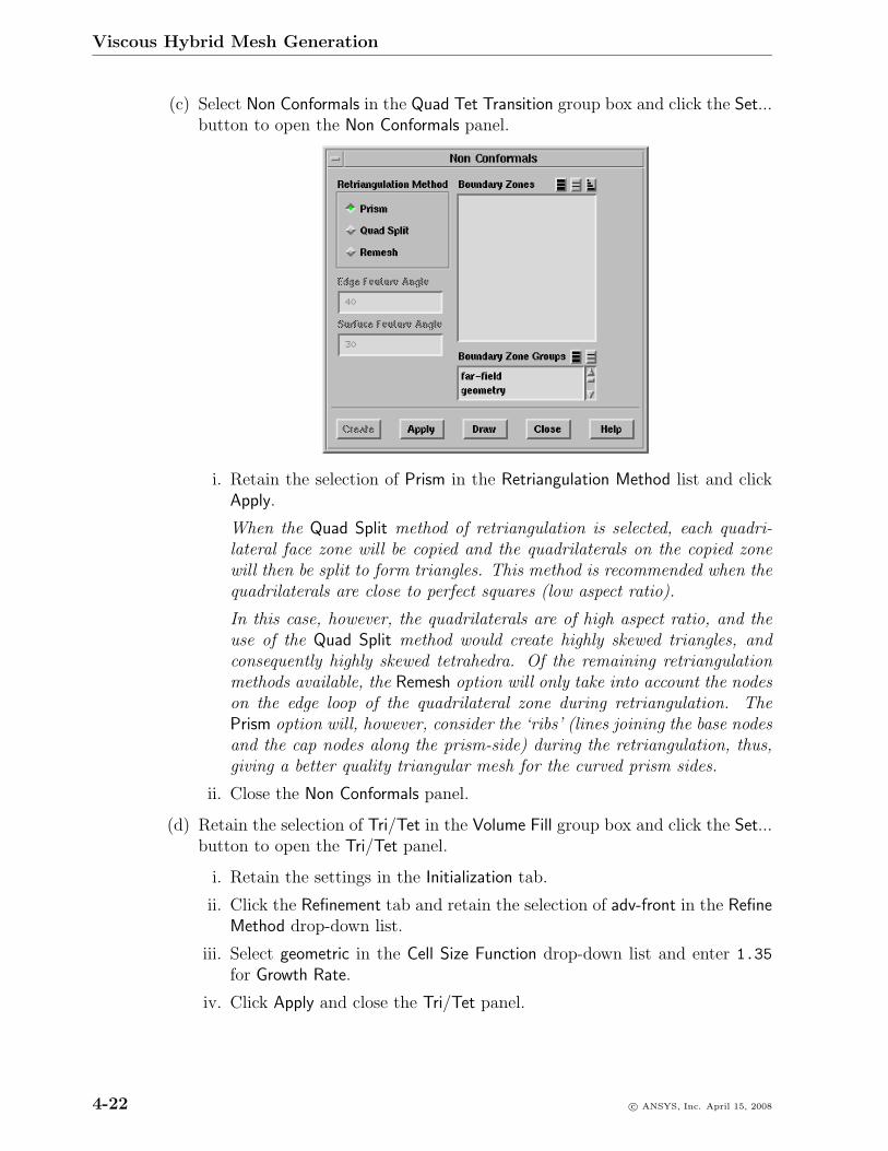
Viscous Hybrid Mesh Generation
(c) Select Non Conformals in the Quad Tet Transition group box and click the Set...button to open the Non Conformals panel.
i. Retain the selection of Prism in the Retriangulation Method list and clickApply.
When the Quad Split method of retriangulation is selected, each quadri-lateral face zone will be copied and the quadrilaterals on the copied zonewill then be split to form triangles. This method is recommended when thequadrilaterals are close to perfect squares (low aspect ratio).
In this case, however, the quadrilaterals are of high aspect ratio, and theuse of the Quad Split method would create highly skewed triangles, andconsequently highly skewed tetrahedra. Of the remaining retriangulationmethods available, the Remesh option will only take into account the nodeson the edge loop of the quadrilateral zone during retriangulation. ThePrism option will, however, consider the ‘ribs’ (lines joining the base nodesand the cap nodes along the prism-side) during the retriangulation, thus,giving a better quality triangular mesh for the curved prism sides.
ii. Close the Non Conformals panel.
(d) Retain the selection of Tri/Tet in the Volume Fill group box and click the Set...button to open the Tri/Tet panel.
i. Retain the settings in the Initialization tab.
ii. Click the Refinement tab and retain the selection of adv-front in the RefineMethod drop-down list.
iii. Select geometric in the Cell Size Function drop-down list and enter 1.35
for Growth Rate.
iv. Click Apply and close the Tri/Tet panel.
4-22 c© ANSYS, Inc. April 15, 2008
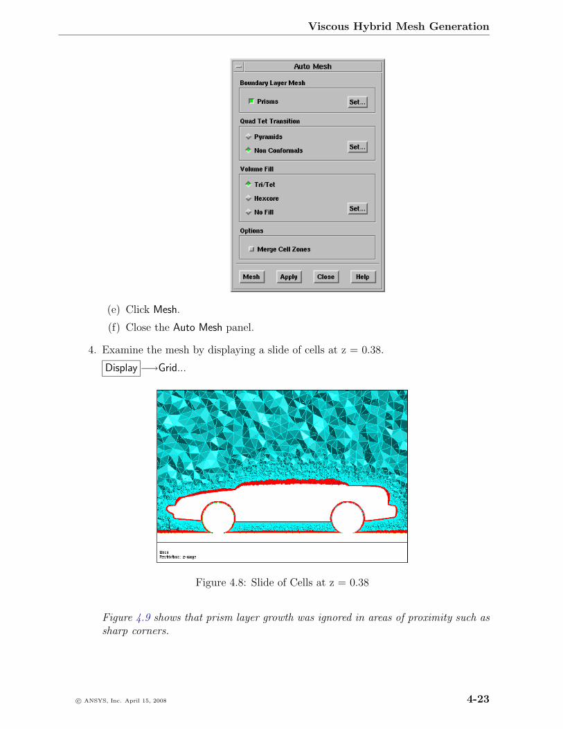
Viscous Hybrid Mesh Generation
(e) Click Mesh.
(f) Close the Auto Mesh panel.
4. Examine the mesh by displaying a slide of cells at z = 0.38.
Display −→Grid...
Figure 4.8: Slide of Cells at z = 0.38
Figure 4.9 shows that prism layer growth was ignored in areas of proximity such assharp corners.
c© ANSYS, Inc. April 15, 2008 4-23
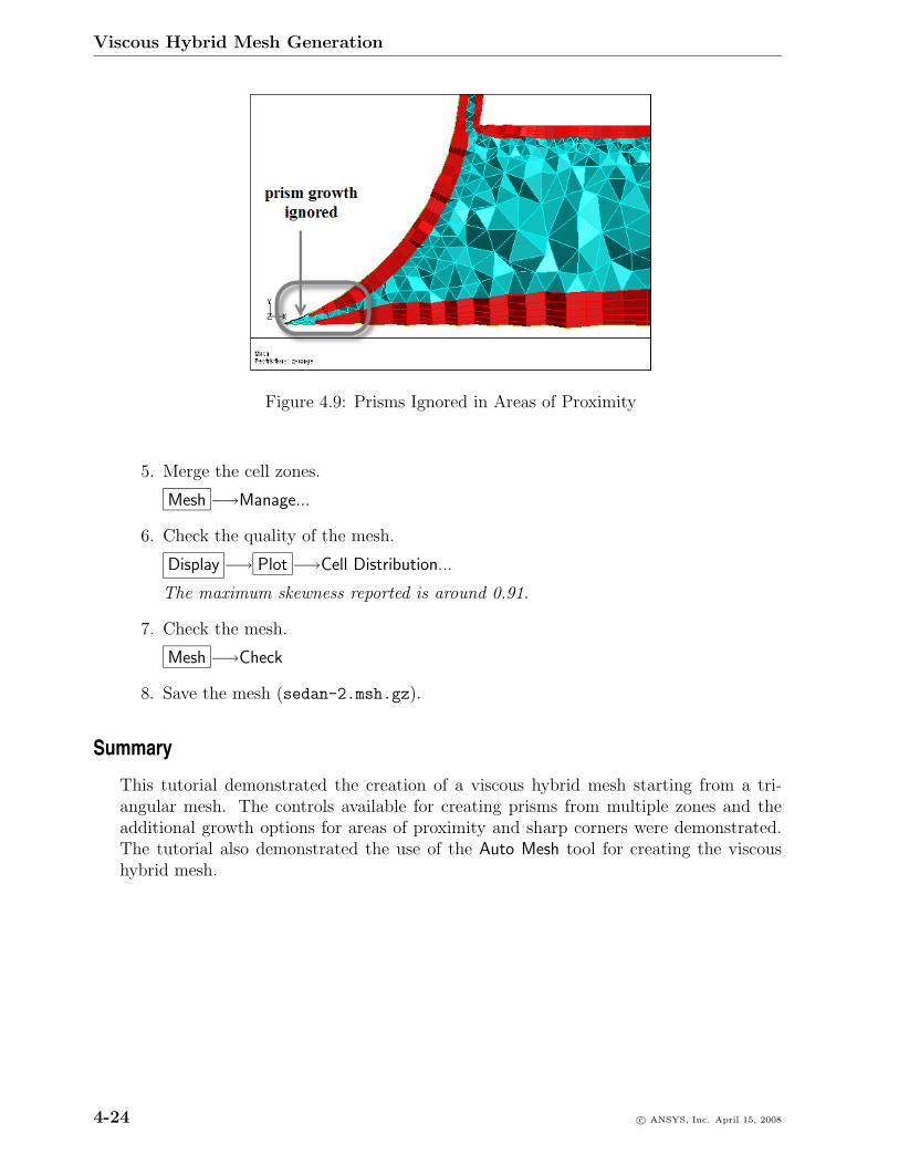
Viscous Hybrid Mesh Generation
Figure 4.9: Prisms Ignored in Areas of Proximity
5. Merge the cell zones.
Mesh −→Manage...
6. Check the quality of the mesh.
Display −→ Plot −→Cell Distribution...
The maximum skewness reported is around 0.91.
7. Check the mesh.
Mesh −→Check
8. Save the mesh (sedan-2.msh.gz).
Summary
This tutorial demonstrated the creation of a viscous hybrid mesh starting from a tri-angular mesh. The controls available for creating prisms from multiple zones and theadditional growth options for areas of proximity and sharp corners were demonstrated.The tutorial also demonstrated the use of the Auto Mesh tool for creating the viscoushybrid mesh.
4-24 c© ANSYS, Inc. April 15, 2008
Tutorial 5. Hexcore Mesh Generation
Introduction
Hexcore meshing is a hybrid meshing scheme which generates Cartesian cells inside thecore of the domain and tetrahedral cells close to the boundaries. Hanging-node refine-ments on the Cartesian cells allow efficient cell size transition from the boundary to theinterior of the domain. Thus, a hexcore mesh can significantly reduce the cell countcompared with a fully tetrahedral mesh. The hexcore meshing scheme is applicable to allvolumes but is useful for volumes with large internal regions and few internal boundaries.It is fully automated and compatible with prism (boundary layer) generation.
Hexcore meshes are more useful in applications with large open spaces. One such appli-cation from the automotive industry is explained here.
This tutorial demonstrates how to do the following:
1. Read and display the mesh.
2. Check and improve the skewness of the surface mesh.
3. Repair the boundary mesh by merging the nodes and splitting the edges of thegeometry.
4. Generate the tetrahedral mesh.
5. Generate the hexcore mesh.
6. Examine the effect of buffer layers on the hexcore mesh.
7. Generate the hexcore mesh in conjuction with boundary layer (prism) meshing andlocal refinement.
Prerequisites
This tutorial assumes that you have some experience with TGrid, and that you are familiarwith the graphical user interface.
c© ANSYS, Inc. April 15, 2008 5-1

Hexcore Mesh Generation
Preparation
1. Download hexcore.zip from the FLUENT User Services Center to your workingdirectory. This file can be found from the Documentation link on the TGrid productpage.
OR
Copy hexcore.zip from the TGrid documentation CD to your working directory.
• For UNIX systems, insert the CD into your CD-ROM drive and go to thefollowing directory:
cdrom/tgrid5.0/help/tutfiles
where, cdrom must be replaced by the name of your CD-ROM drive.
• For Windows systems, insert the CD into your CD-ROM drive and go to thefollowing folder:
cdrom:\tgrid5.0\help\tutfiles
where, cdrom must be replaced by the name of your CD-ROM drive (e.g., E).
2. Unzip hexcore.zip.
The file, cabin-hvac.msh can be found in the hexcore folder created on unzippingthe file.
3. Start the 3D (3d) version of TGrid.
5-2 c© ANSYS, Inc. April 15, 2008
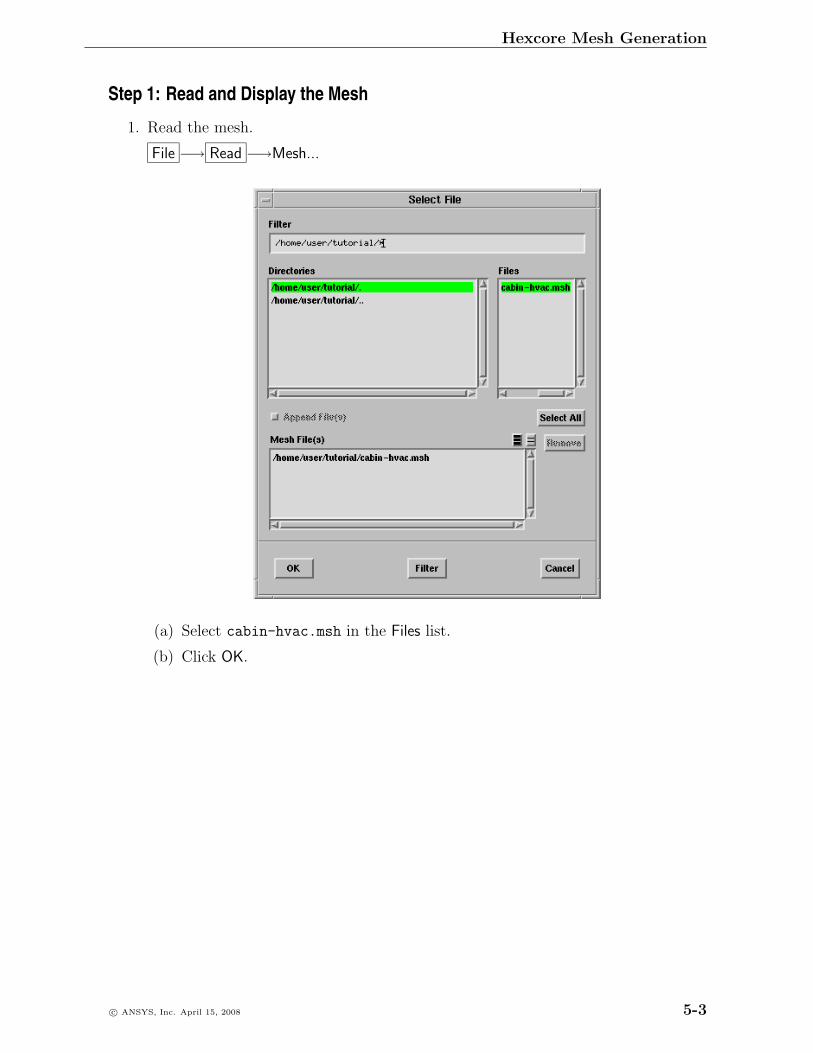
Hexcore Mesh Generation
Step 1: Read and Display the Mesh
1. Read the mesh.
File −→ Read −→Mesh...
(a) Select cabin-hvac.msh in the Files list.
(b) Click OK.
c© ANSYS, Inc. April 15, 2008 5-3
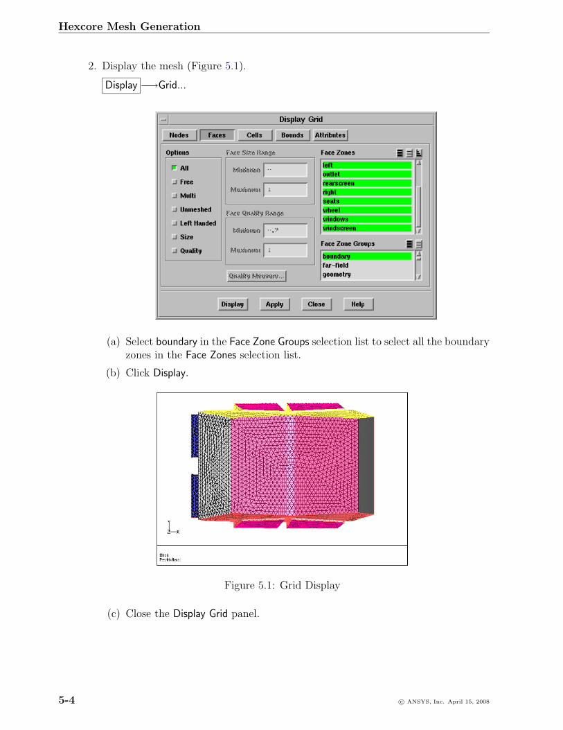
Hexcore Mesh Generation
2. Display the mesh (Figure 5.1).
Display −→Grid...
(a) Select boundary in the Face Zone Groups selection list to select all the boundaryzones in the Face Zones selection list.
(b) Click Display.
Figure 5.1: Grid Display
(c) Close the Display Grid panel.
5-4 c© ANSYS, Inc. April 15, 2008
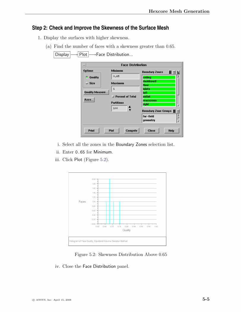
Hexcore Mesh Generation
Step 2: Check and Improve the Skewness of the Surface Mesh
1. Display the surfaces with higher skewness.
(a) Find the number of faces with a skewness greater than 0.65.
Display −→ Plot −→Face Distribution...
i. Select all the zones in the Boundary Zones selection list.
ii. Enter 0.65 for Minimum.
iii. Click Plot (Figure 5.2).
Figure 5.2: Skewness Distribution Above 0.65
iv. Close the Face Distribution panel.
c© ANSYS, Inc. April 15, 2008 5-5
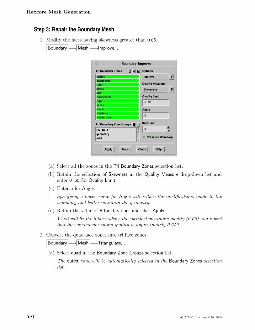
Hexcore Mesh Generation
Step 3: Repair the Boundary Mesh
1. Modify the faces having skewness greater than 0.65.
Boundary −→ Mesh −→Improve...
(a) Select all the zones in the Tri Boundary Zones selection list.
(b) Retain the selection of Skewness in the Quality Measure drop-down list andenter 0.65 for Quality Limit.
(c) Enter 5 for Angle.
Specifying a lower value for Angle will reduce the modifications made to theboundary and better maintain the geometry.
(d) Retain the value of 5 for Iterations and click Apply.
TGrid will fix the 6 faces above the specified maximum quality (0.65) and reportthat the current maximum quality is approximately 0.649.
2. Convert the quad face zones into tri face zones.
Boundary −→ Mesh −→Triangulate...
(a) Select quad in the Boundary Zone Groups selection list.
The outlet zone will be automatically selected in the Boundary Zones selectionlist.
5-6 c© ANSYS, Inc. April 15, 2008
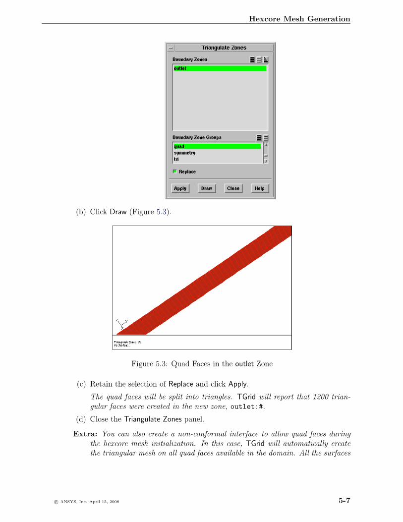
Hexcore Mesh Generation
(b) Click Draw (Figure 5.3).
Figure 5.3: Quad Faces in the outlet Zone
(c) Retain the selection of Replace and click Apply.
The quad faces will be split into triangles. TGrid will report that 1200 trian-gular faces were created in the new zone, outlet:#.
(d) Close the Triangulate Zones panel.
Extra: You can also create a non-conformal interface to allow quad faces duringthe hexcore mesh initialization. In this case, TGrid will automatically createthe triangular mesh on all quad faces available in the domain. All the surfaces
c© ANSYS, Inc. April 15, 2008 5-7

Hexcore Mesh Generation
having quad elements will be copied and remeshed with triangular cells. Thefree nodes of the triangular mesh will be merged with the original surface mesh.
3. Check the quality of the surface mesh.
(a) Select all the zones in the Tri Boundary Zones selection list in the BoundaryImprove panel.
(b) Retain the selection of Skewness in the Quality Measure drop-down list and0.65 for Quality Limit.
(c) Click Apply.
The maximum skewness reported is still less than 0.65, hence the mesh isacceptable.
(d) Close the Boundary Improve panel.
4. Save the mesh file.
File −→ Write −→Mesh...
Step 4: Generate the Tetrahedral Mesh
1. Generate a tetrahedral mesh with the default settings.
Mesh −→Tri/Tet...
(a) Enable Delete Dead Zones in the Tri Tet Zones group box.
(b) Retain the default settings for the remaining parameters and click Init&Refine.
The number of cells generated is approximately 204763 while the maximumskewness reported is around 0.856. The exact number may vary slightly ondifferent platforms.
(c) Close the Tri/Tet panel.
2. Display a slide of cells at y = 50.
Display −→Grid...
(a) Retain the selection of all the boundary zones in the Face Zones selection list.
(b) Click the Bounds tab and click Compute.
5-8 c© ANSYS, Inc. April 15, 2008
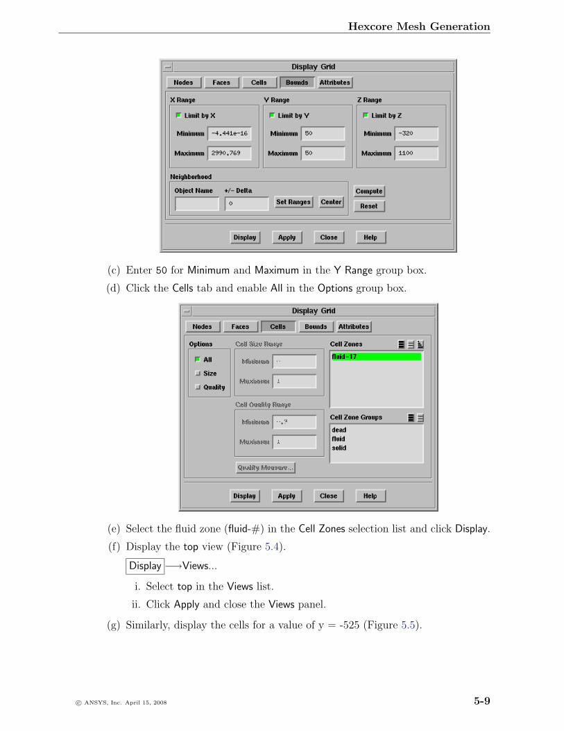
Hexcore Mesh Generation
(c) Enter 50 for Minimum and Maximum in the Y Range group box.
(d) Click the Cells tab and enable All in the Options group box.
(e) Select the fluid zone (fluid-#) in the Cell Zones selection list and click Display.
(f) Display the top view (Figure 5.4).
Display −→Views...
i. Select top in the Views list.
ii. Click Apply and close the Views panel.
(g) Similarly, display the cells for a value of y = -525 (Figure 5.5).
c© ANSYS, Inc. April 15, 2008 5-9
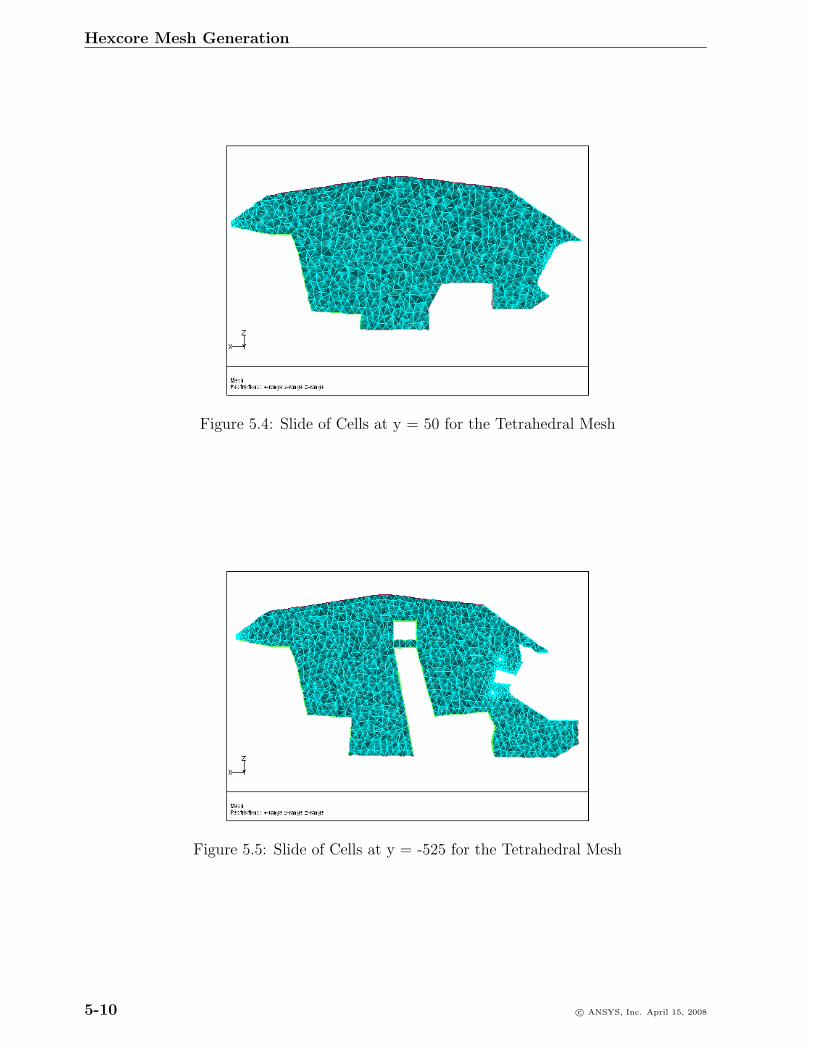
Hexcore Mesh Generation
Figure 5.4: Slide of Cells at y = 50 for the Tetrahedral Mesh
Figure 5.5: Slide of Cells at y = -525 for the Tetrahedral Mesh
5-10 c© ANSYS, Inc. April 15, 2008
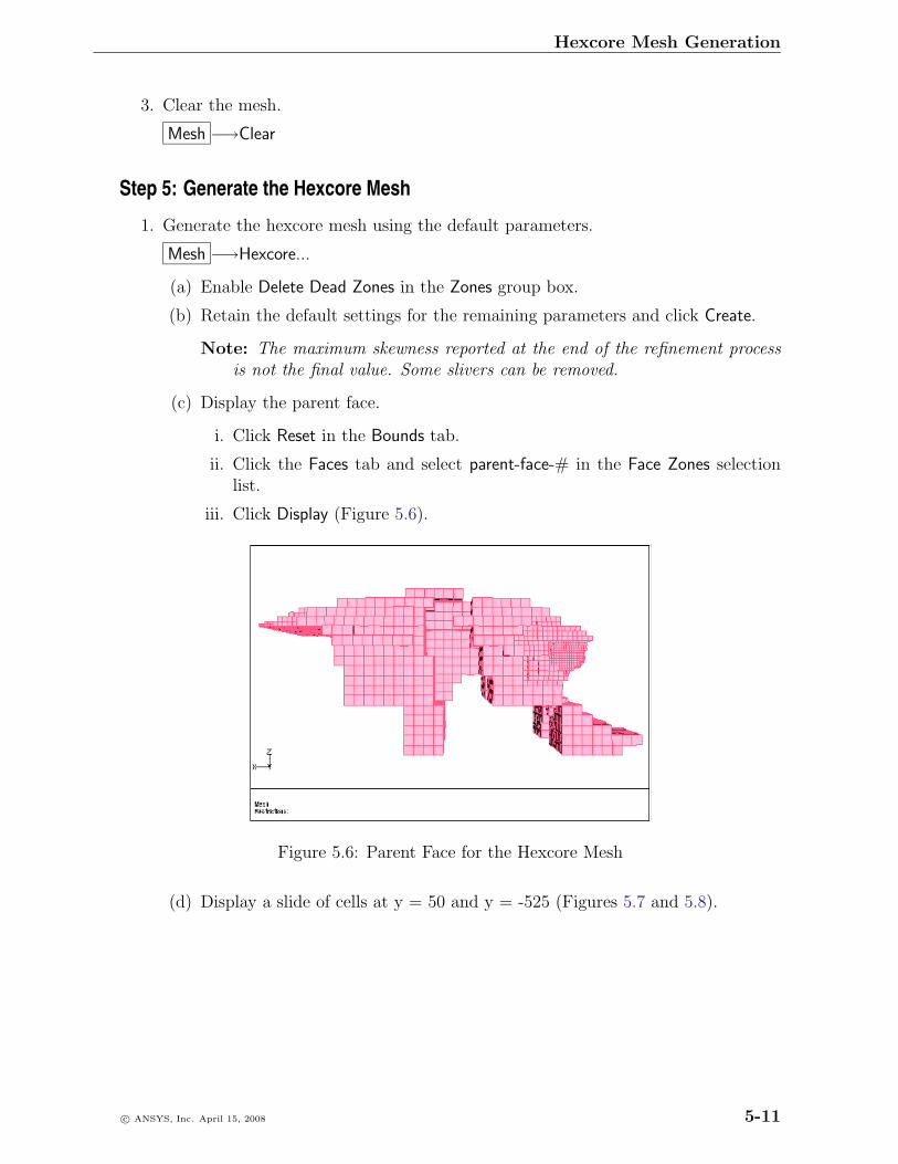
Hexcore Mesh Generation
3. Clear the mesh.
Mesh −→Clear
Step 5: Generate the Hexcore Mesh
1. Generate the hexcore mesh using the default parameters.
Mesh −→Hexcore...
(a) Enable Delete Dead Zones in the Zones group box.
(b) Retain the default settings for the remaining parameters and click Create.
Note: The maximum skewness reported at the end of the refinement processis not the final value. Some slivers can be removed.
(c) Display the parent face.
i. Click Reset in the Bounds tab.
ii. Click the Faces tab and select parent-face-# in the Face Zones selectionlist.
iii. Click Display (Figure 5.6).
Figure 5.6: Parent Face for the Hexcore Mesh
(d) Display a slide of cells at y = 50 and y = -525 (Figures 5.7 and 5.8).
c© ANSYS, Inc. April 15, 2008 5-11

Hexcore Mesh Generation
Figure 5.7: Slide of Cells at y = 50 for the Hexcore Mesh With Buffer Layers = 1
Figure 5.8: Slide of Cells at y = -525 for the Hexcore Mesh With Buffer Layers = 1
5-12 c© ANSYS, Inc. April 15, 2008
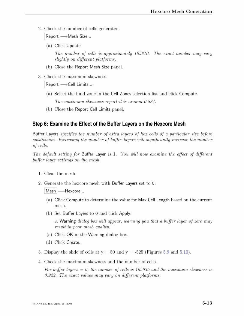
Hexcore Mesh Generation
2. Check the number of cells generated.
Report −→Mesh Size...
(a) Click Update.
The number of cells is approximately 185810. The exact number may varyslightly on different platforms.
(b) Close the Report Mesh Size panel.
3. Check the maximum skewness.
Report −→Cell Limits...
(a) Select the fluid zone in the Cell Zones selection list and click Compute.
The maximum skewness reported is around 0.884.
(b) Close the Report Cell Limits panel.
Step 6: Examine the Effect of the Buffer Layers on the Hexcore Mesh
Buffer Layers specifies the number of extra layers of hex cells of a particular size beforesubdivision. Increasing the number of buffer layers will significantly increase the numberof cells.
The default setting for Buffer Layer is 1. You will now examine the effect of differentbuffer layer settings on the mesh.
1. Clear the mesh.
2. Generate the hexcore mesh with Buffer Layers set to 0.
Mesh −→Hexcore...
(a) Click Compute to determine the value for Max Cell Length based on the currentmesh.
(b) Set Buffer Layers to 0 and click Apply.
A Warning dialog box will appear, warning you that a buffer layer of zero mayresult in poor mesh quality.
(c) Click OK in the Warning dialog box.
(d) Click Create.
3. Display the slide of cells at y = 50 and y = -525 (Figures 5.9 and 5.10).
4. Check the maximum skewness and the number of cells.
For buffer layers = 0, the number of cells is 165035 and the maximum skewness is0.922. The exact values may vary on different platforms.
c© ANSYS, Inc. April 15, 2008 5-13
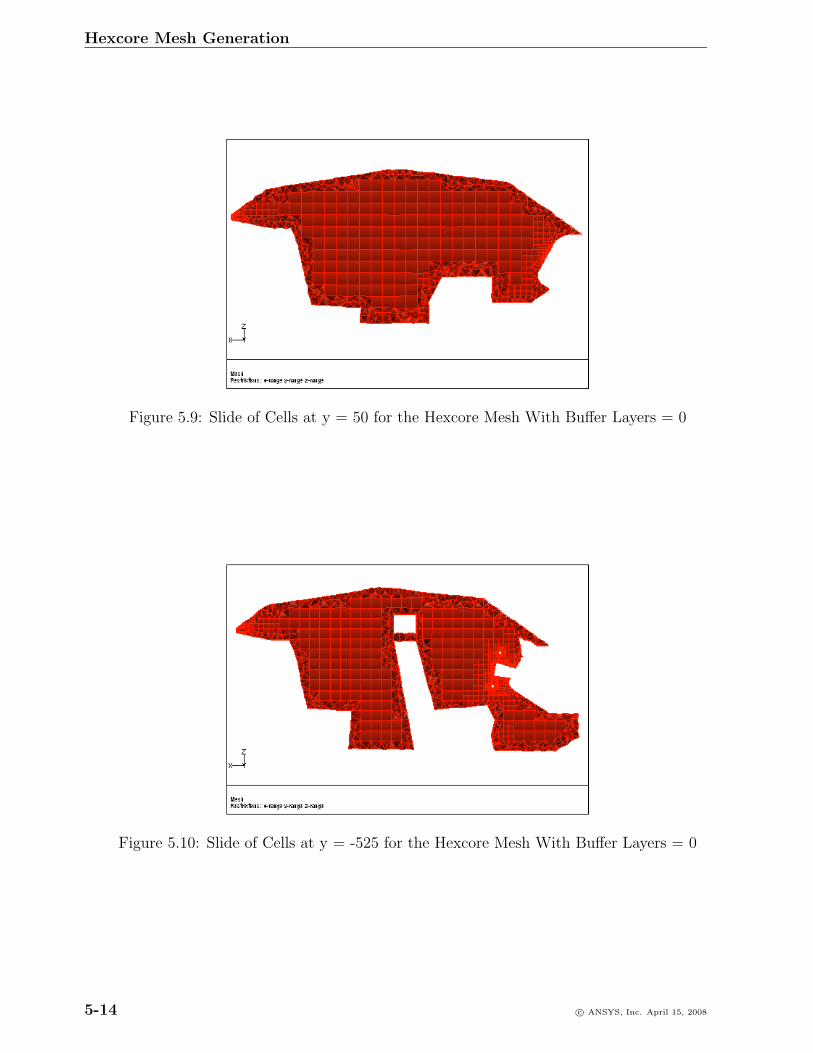
Hexcore Mesh Generation
Figure 5.9: Slide of Cells at y = 50 for the Hexcore Mesh With Buffer Layers = 0
Figure 5.10: Slide of Cells at y = -525 for the Hexcore Mesh With Buffer Layers = 0
5-14 c© ANSYS, Inc. April 15, 2008
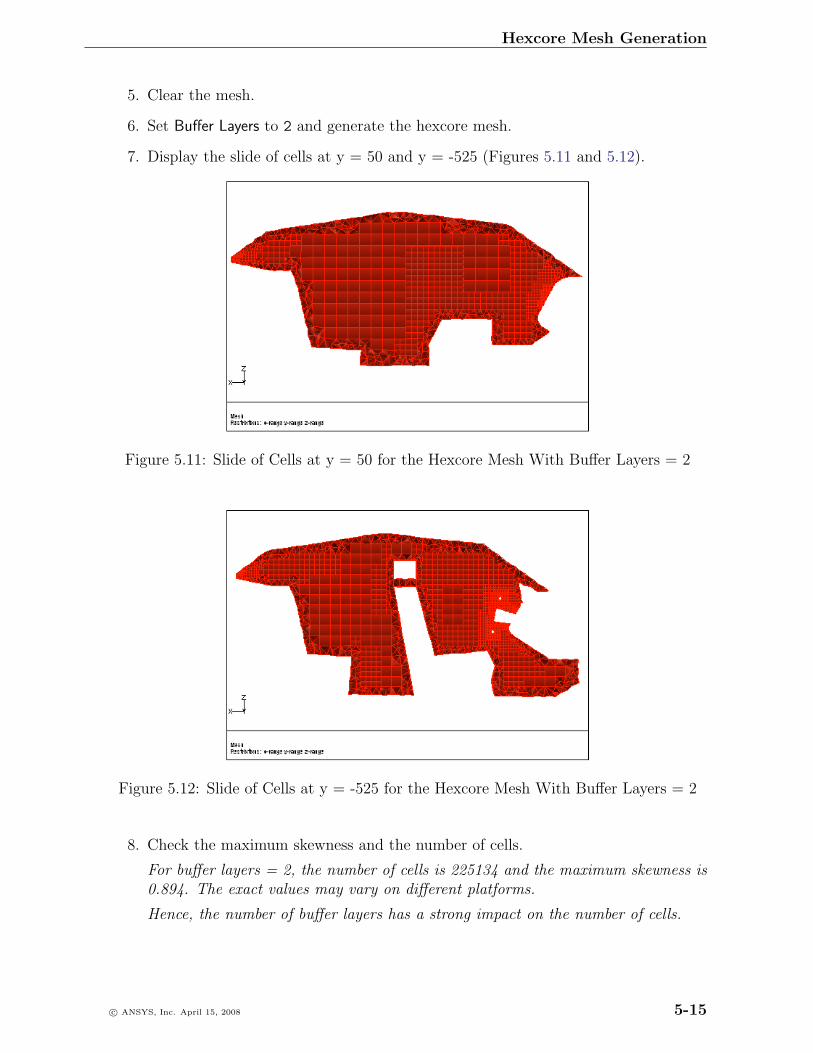
Hexcore Mesh Generation
5. Clear the mesh.
6. Set Buffer Layers to 2 and generate the hexcore mesh.
7. Display the slide of cells at y = 50 and y = -525 (Figures 5.11 and 5.12).
Figure 5.11: Slide of Cells at y = 50 for the Hexcore Mesh With Buffer Layers = 2
Figure 5.12: Slide of Cells at y = -525 for the Hexcore Mesh With Buffer Layers = 2
8. Check the maximum skewness and the number of cells.
For buffer layers = 2, the number of cells is 225134 and the maximum skewness is0.894. The exact values may vary on different platforms.
Hence, the number of buffer layers has a strong impact on the number of cells.
c© ANSYS, Inc. April 15, 2008 5-15
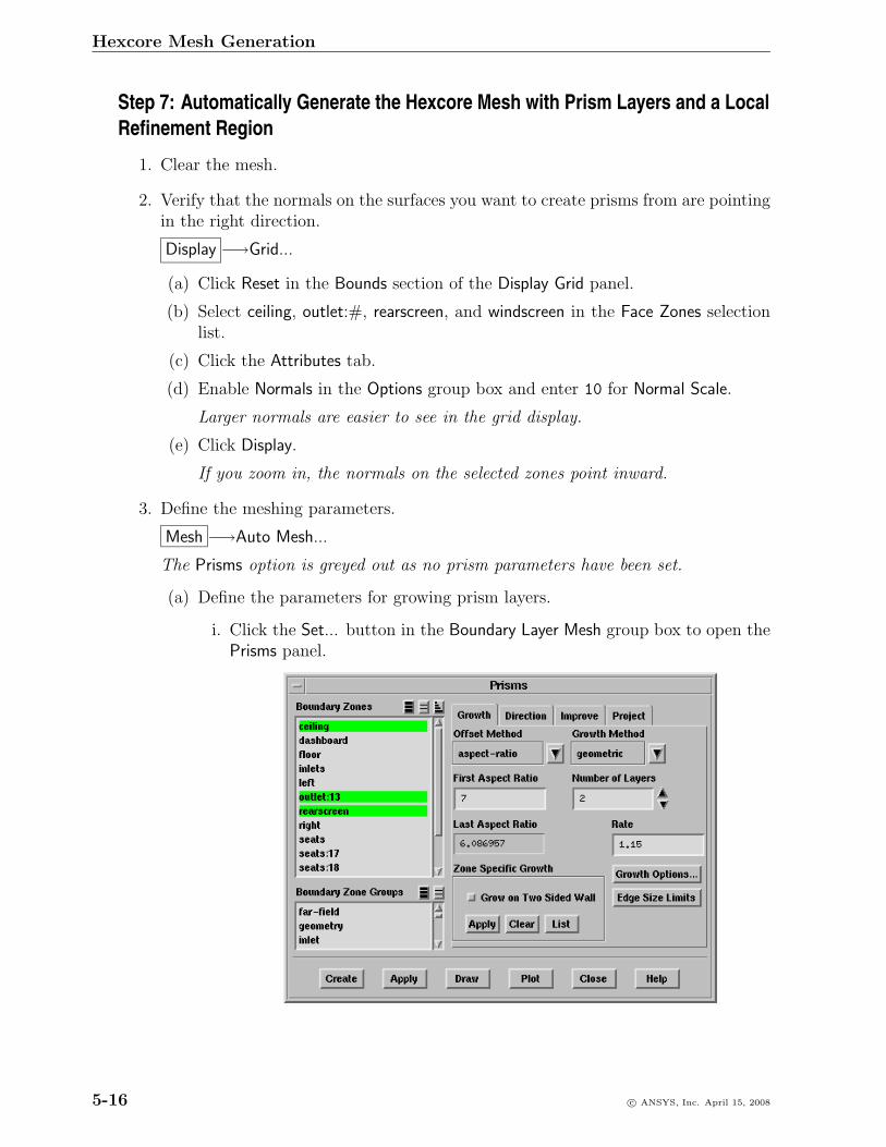
Hexcore Mesh Generation
Step 7: Automatically Generate the Hexcore Mesh with Prism Layers and a LocalRefinement Region
1. Clear the mesh.
2. Verify that the normals on the surfaces you want to create prisms from are pointingin the right direction.
Display −→Grid...
(a) Click Reset in the Bounds section of the Display Grid panel.
(b) Select ceiling, outlet:#, rearscreen, and windscreen in the Face Zones selectionlist.
(c) Click the Attributes tab.
(d) Enable Normals in the Options group box and enter 10 for Normal Scale.
Larger normals are easier to see in the grid display.
(e) Click Display.
If you zoom in, the normals on the selected zones point inward.
3. Define the meshing parameters.
Mesh −→Auto Mesh...
The Prisms option is greyed out as no prism parameters have been set.
(a) Define the parameters for growing prism layers.
i. Click the Set... button in the Boundary Layer Mesh group box to open thePrisms panel.
5-16 c© ANSYS, Inc. April 15, 2008

Hexcore Mesh Generation
ii. Select ceiling, outlet:#, rearscreen, and windscreen in the Boundary Zonesselection list.
iii. Select aspect-ratio in the Offset Method drop-down list and enter 7 for FirstAspect Ratio.
iv. Select geometric in the Growth Method drop-down list and set the Numberof Layers to 2.
v. Enter 1.15 for Rate.
vi. Click Apply in the Zone Specific Growth group box.
! It is necessary to apply the prism growth parameters on specific zones forTGrid to retain the growth parameters in memory. The Prisms option in theAuto Mesh panel will be visible only after applying zone-specific growth.
vii. Close the Prisms panel.
viii. Enable Prisms in the Boundary Layer Mesh group box in the Auto Meshpanel.
(b) Display all the surfaces except right using the Display Grid panel.
Make sure the display of normals is disabled in the Attributes tab.
(c) Define the parameters for hexcore meshing.
i. Select Hexcore in the Volume Fill list in the Auto Mesh panel and click theSet... button to open the Hexcore panel.
ii. Compute the average length of the faces on the ceiling zone.
A. Zoom in to the ceiling zone in the graphics display.
B. Use the hot-key Ctrl + N to enable the selection of nodes.
C. Select two adjacent nodes using the right mouse button.
D. Use the hot-key Ctrl + D to calculate the distance between the selectednodes.
The distance between the nodes is computed to be approximately 75.
iii. Enter 120 for Max Cell Length.
This is the maximum length for the hexahedral cells in the volume mesh.
iv. Set Buffer Layers to 1.
c© ANSYS, Inc. April 15, 2008 5-17
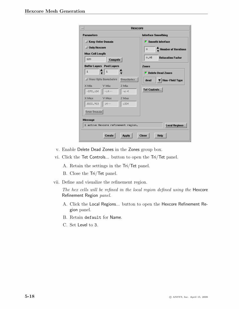
Hexcore Mesh Generation
v. Enable Delete Dead Zones in the Zones group box.
vi. Click the Tet Controls... button to open the Tri/Tet panel.
A. Retain the settings in the Tri/Tet panel.
B. Close the Tri/Tet panel.
vii. Define and visualize the refinement region.
The hex cells will be refined in the local region defined using the HexcoreRefinement Region panel.
A. Click the Local Regions... button to open the Hexcore Refinement Re-gion panel.
B. Retain default for Name.
C. Set Level to 3.
5-18 c© ANSYS, Inc. April 15, 2008
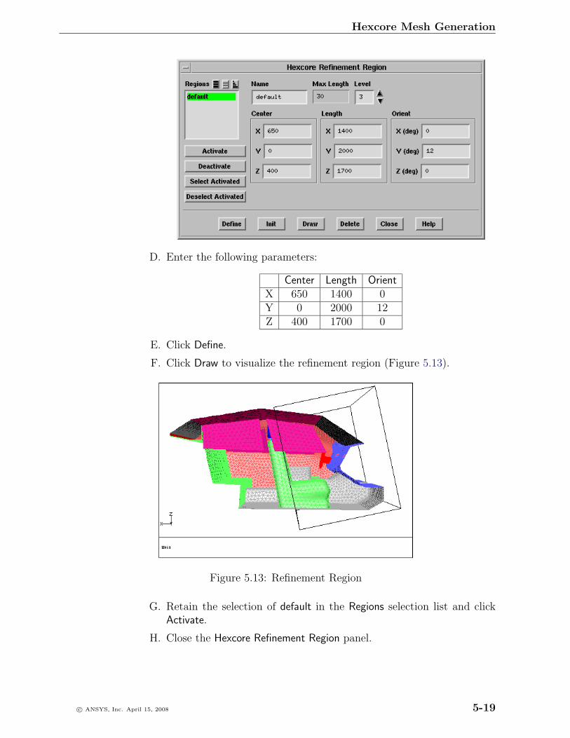
Hexcore Mesh Generation
D. Enter the following parameters:
Center Length OrientX 650 1400 0Y 0 2000 12Z 400 1700 0
E. Click Define.
F. Click Draw to visualize the refinement region (Figure 5.13).
Figure 5.13: Refinement Region
G. Retain the selection of default in the Regions selection list and clickActivate.
H. Close the Hexcore Refinement Region panel.
c© ANSYS, Inc. April 15, 2008 5-19
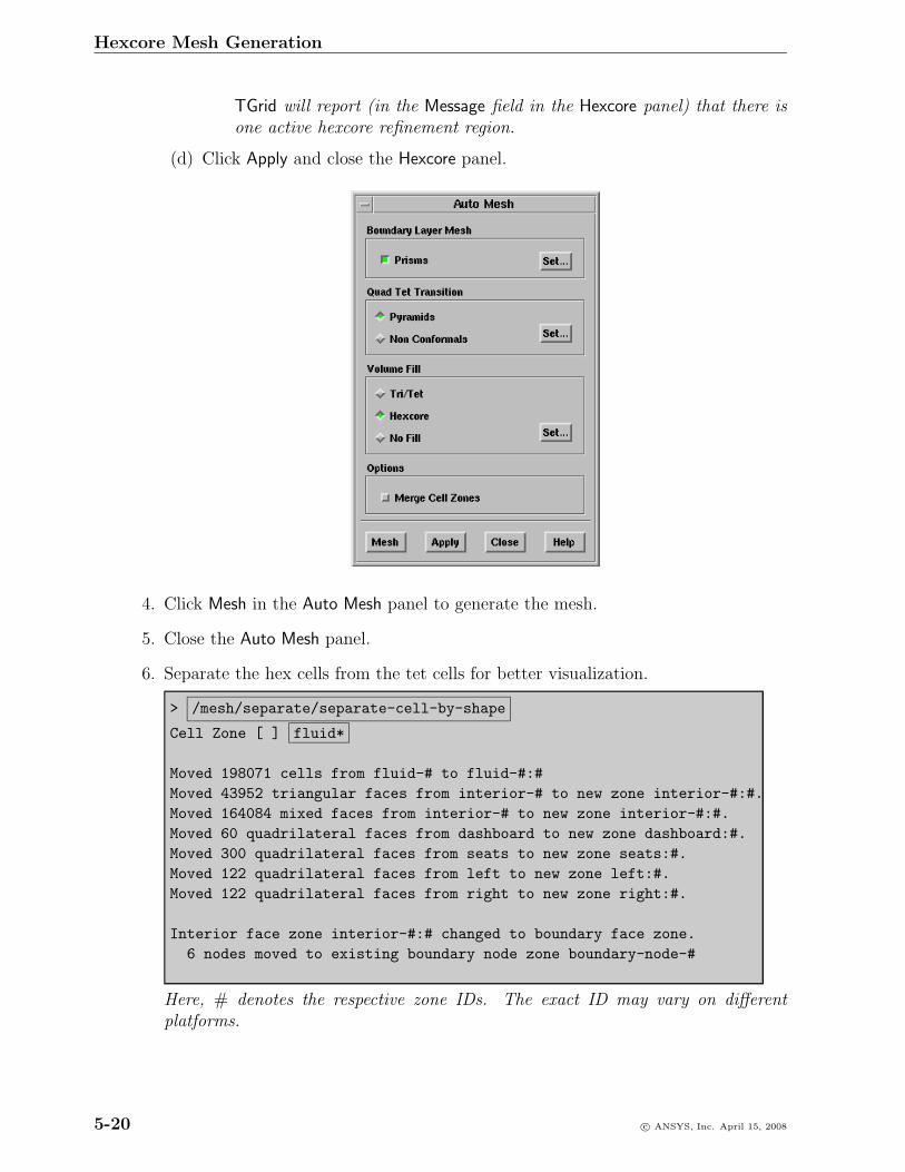
Hexcore Mesh Generation
TGrid will report (in the Message field in the Hexcore panel) that there isone active hexcore refinement region.
(d) Click Apply and close the Hexcore panel.
4. Click Mesh in the Auto Mesh panel to generate the mesh.
5. Close the Auto Mesh panel.
6. Separate the hex cells from the tet cells for better visualization.
> /mesh/separate/separate-cell-by-shape
Cell Zone [ ] fluid*
Moved 198071 cells from fluid-# to fluid-#:#Moved 43952 triangular faces from interior-# to new zone interior-#:#.Moved 164084 mixed faces from interior-# to new zone interior-#:#.Moved 60 quadrilateral faces from dashboard to new zone dashboard:#.Moved 300 quadrilateral faces from seats to new zone seats:#.Moved 122 quadrilateral faces from left to new zone left:#.Moved 122 quadrilateral faces from right to new zone right:#.
Interior face zone interior-#:# changed to boundary face zone.6 nodes moved to existing boundary node zone boundary-node-#
Here, # denotes the respective zone IDs. The exact ID may vary on differentplatforms.
5-20 c© ANSYS, Inc. April 15, 2008
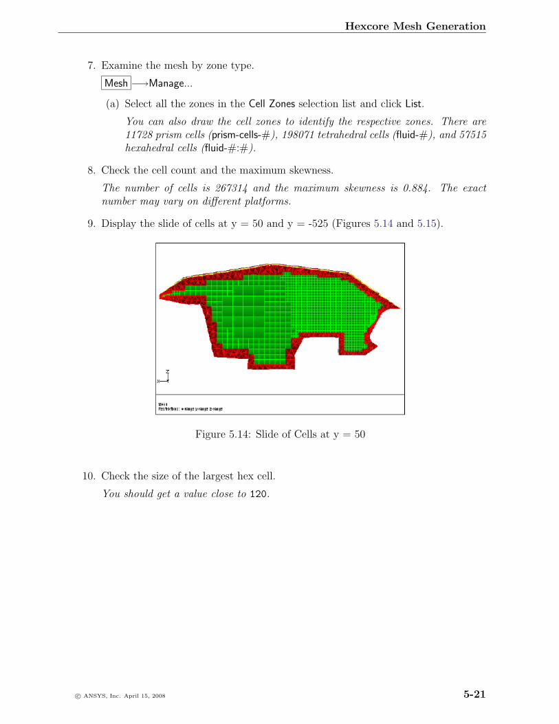
Hexcore Mesh Generation
7. Examine the mesh by zone type.
Mesh −→Manage...
(a) Select all the zones in the Cell Zones selection list and click List.
You can also draw the cell zones to identify the respective zones. There are11728 prism cells (prism-cells-#), 198071 tetrahedral cells (fluid-#), and 57515hexahedral cells (fluid-#:#).
8. Check the cell count and the maximum skewness.
The number of cells is 267314 and the maximum skewness is 0.884. The exactnumber may vary on different platforms.
9. Display the slide of cells at y = 50 and y = -525 (Figures 5.14 and 5.15).
Figure 5.14: Slide of Cells at y = 50
10. Check the size of the largest hex cell.
You should get a value close to 120.
c© ANSYS, Inc. April 15, 2008 5-21
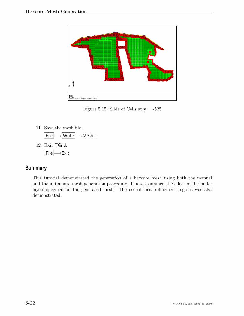
Hexcore Mesh Generation
Figure 5.15: Slide of Cells at y = -525
11. Save the mesh file.
File −→ Write −→Mesh...
12. Exit TGrid.
File −→Exit
Summary
This tutorial demonstrated the generation of a hexcore mesh using both the manualand the automatic mesh generation procedure. It also examined the effect of the bufferlayers specified on the generated mesh. The use of local refinement regions was alsodemonstrated.
5-22 c© ANSYS, Inc. April 15, 2008
Tutorial 6. Generating the Hexcore Mesh Upto DomainBoundaries
Introduction
When generating the hexcore mesh for external flow domains, it may not be necessary tohave a tetrahedral mesh at the domain boundaries. For such cases, you can generate thehexcore mesh until the domain boundaries, thereby also reducing the cell count. Thistutorial demonstrates the generation of the hexcore mesh upto the domain boundariesfor a sedan car.
This tutorial demonstrates how to do the following:
1. Read the mesh file and display the boundary mesh.
2. Set parameters for generating the hexcore mesh.
3. Set parameters for creating prism layers and the hexcore mesh using automaticmeshing.
4. Check and save the volume mesh.
Prerequisites
This tutorial assumes that you have some experience with TGrid, and that you are familiarwith the graphical user interface.
Preparation
1. Download hexcore-boundaries.zip from the FLUENT User Services Center toyour working directory. This file can be found from the Documentation link on theTGrid product page.
OR
Copy hexcore-boundaries.zip from the TGrid documentation CD to your work-ing directory.
c© ANSYS, Inc. April 15, 2008 6-1
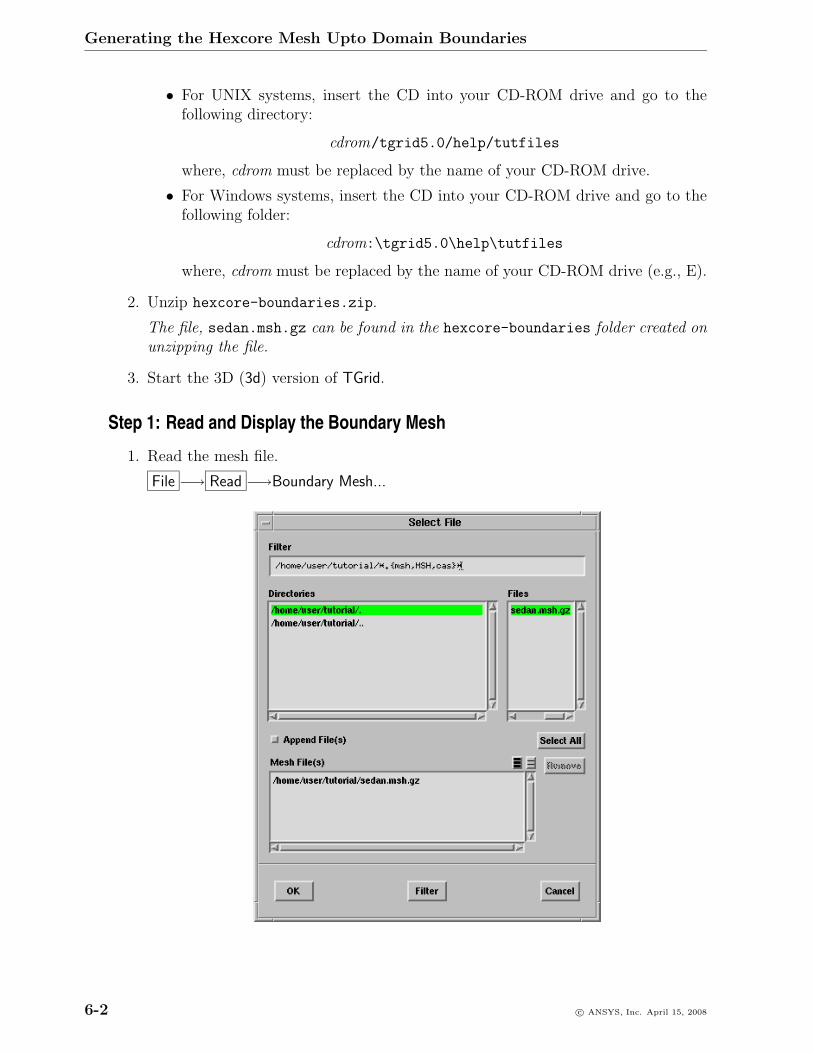
Generating the Hexcore Mesh Upto Domain Boundaries
• For UNIX systems, insert the CD into your CD-ROM drive and go to thefollowing directory:
cdrom/tgrid5.0/help/tutfiles
where, cdrom must be replaced by the name of your CD-ROM drive.
• For Windows systems, insert the CD into your CD-ROM drive and go to thefollowing folder:
cdrom:\tgrid5.0\help\tutfiles
where, cdrom must be replaced by the name of your CD-ROM drive (e.g., E).
2. Unzip hexcore-boundaries.zip.
The file, sedan.msh.gz can be found in the hexcore-boundaries folder created onunzipping the file.
3. Start the 3D (3d) version of TGrid.
Step 1: Read and Display the Boundary Mesh
1. Read the mesh file.
File −→ Read −→Boundary Mesh...
6-2 c© ANSYS, Inc. April 15, 2008
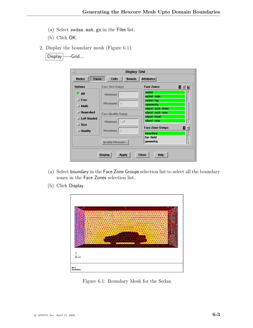
Generating the Hexcore Mesh Upto Domain Boundaries
(a) Select sedan.msh.gz in the Files list.
(b) Click OK.
2. Display the boundary mesh (Figure 6.1).
Display −→Grid...
(a) Select boundary in the Face Zone Groups selection list to select all the boundaryzones in the Face Zones selection list.
(b) Click Display.
Figure 6.1: Boundary Mesh for the Sedan
c© ANSYS, Inc. April 15, 2008 6-3
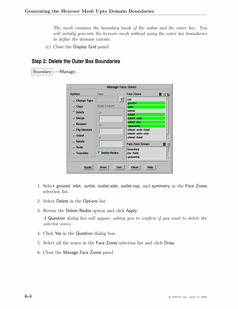
Generating the Hexcore Mesh Upto Domain Boundaries
The mesh contains the boundary mesh of the sedan and the outer box. Youwill initally generate the hexcore mesh without using the outer box boundariesto define the domain extents.
(c) Close the Display Grid panel.
Step 2: Delete the Outer Box Boundaries
Boundary −→Manage...
1. Select ground, inlet, outlet, outlet-side, outlet-top, and symmetry in the Face Zonesselection list.
2. Select Delete in the Options list.
3. Retain the Delete Nodes option and click Apply.
A Question dialog box will appear, asking you to confirm if you want to delete theselected zones.
4. Click Yes in the Question dialog box.
5. Select all the zones in the Face Zones selection list and click Draw.
6. Close the Manage Face Zones panel.
6-4 c© ANSYS, Inc. April 15, 2008
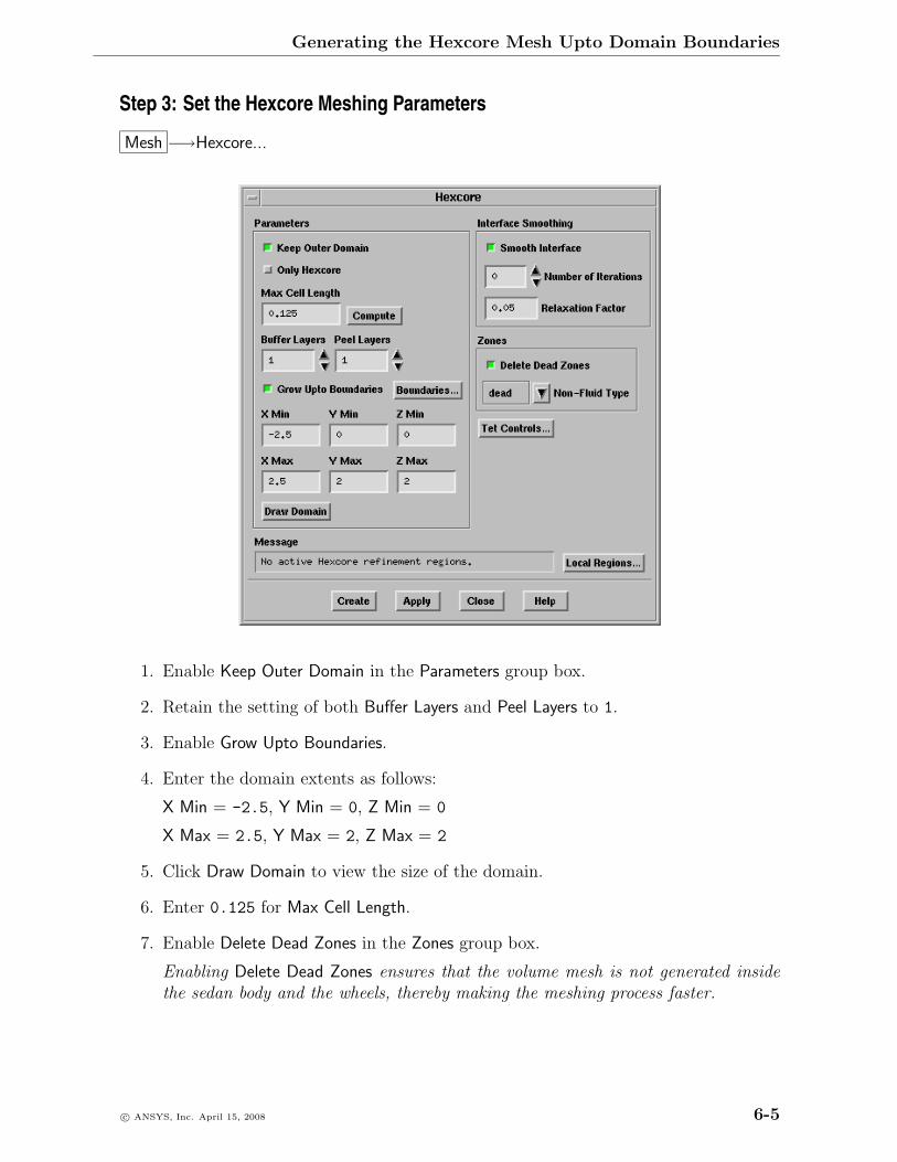
Generating the Hexcore Mesh Upto Domain Boundaries
Step 3: Set the Hexcore Meshing Parameters
Mesh −→Hexcore...
1. Enable Keep Outer Domain in the Parameters group box.
2. Retain the setting of both Buffer Layers and Peel Layers to 1.
3. Enable Grow Upto Boundaries.
4. Enter the domain extents as follows:
X Min = -2.5, Y Min = 0, Z Min = 0
X Max = 2.5, Y Max = 2, Z Max = 2
5. Click Draw Domain to view the size of the domain.
6. Enter 0.125 for Max Cell Length.
7. Enable Delete Dead Zones in the Zones group box.
Enabling Delete Dead Zones ensures that the volume mesh is not generated insidethe sedan body and the wheels, thereby making the meshing process faster.
c© ANSYS, Inc. April 15, 2008 6-5
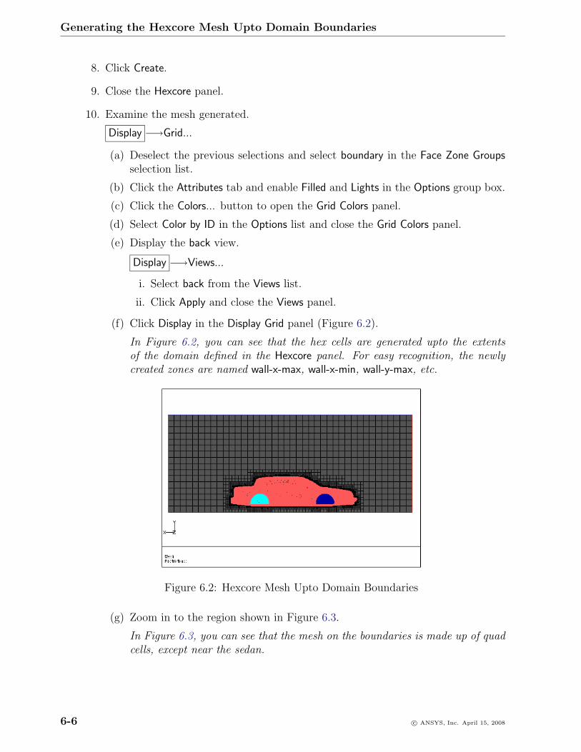
Generating the Hexcore Mesh Upto Domain Boundaries
8. Click Create.
9. Close the Hexcore panel.
10. Examine the mesh generated.
Display −→Grid...
(a) Deselect the previous selections and select boundary in the Face Zone Groupsselection list.
(b) Click the Attributes tab and enable Filled and Lights in the Options group box.
(c) Click the Colors... button to open the Grid Colors panel.
(d) Select Color by ID in the Options list and close the Grid Colors panel.
(e) Display the back view.
Display −→Views...
i. Select back from the Views list.
ii. Click Apply and close the Views panel.
(f) Click Display in the Display Grid panel (Figure 6.2).
In Figure 6.2, you can see that the hex cells are generated upto the extentsof the domain defined in the Hexcore panel. For easy recognition, the newlycreated zones are named wall-x-max, wall-x-min, wall-y-max, etc.
Figure 6.2: Hexcore Mesh Upto Domain Boundaries
(g) Zoom in to the region shown in Figure 6.3.
In Figure 6.3, you can see that the mesh on the boundaries is made up of quadcells, except near the sedan.
6-6 c© ANSYS, Inc. April 15, 2008
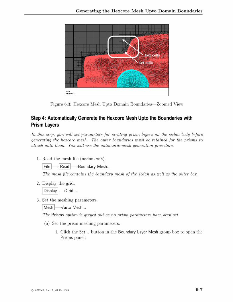
Generating the Hexcore Mesh Upto Domain Boundaries
Figure 6.3: Hexcore Mesh Upto Domain Boundaries—Zoomed View
Step 4: Automatically Generate the Hexcore Mesh Upto the Boundaries withPrism Layers
In this step, you will set parameters for creating prism layers on the sedan body beforegenerating the hexcore mesh. The outer boundaries must be retained for the prisms toattach onto them. You will use the automatic mesh generation procedure.
1. Read the mesh file (sedan.msh).
File −→ Read −→Boundary Mesh...
The mesh file contains the boundary mesh of the sedan as well as the outer box.
2. Display the grid.
Display −→Grid...
3. Set the meshing parameters.
Mesh −→Auto Mesh...
The Prisms option is greyed out as no prism parameters have been set.
(a) Set the prism meshing parameters.
i. Click the Set... button in the Boundary Layer Mesh group box to open thePrisms panel.
c© ANSYS, Inc. April 15, 2008 6-7
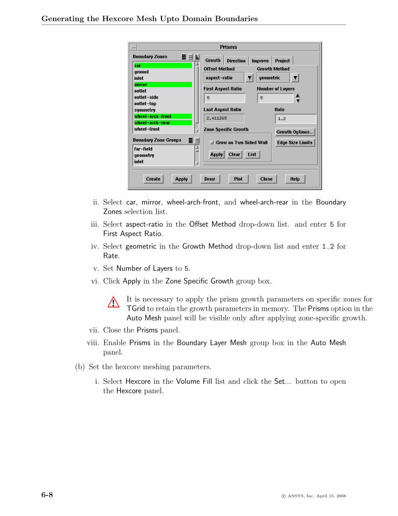
Generating the Hexcore Mesh Upto Domain Boundaries
ii. Select car, mirror, wheel-arch-front, and wheel-arch-rear in the BoundaryZones selection list.
iii. Select aspect-ratio in the Offset Method drop-down list. and enter 5 forFirst Aspect Ratio.
iv. Select geometric in the Growth Method drop-down list and enter 1.2 forRate.
v. Set Number of Layers to 5.
vi. Click Apply in the Zone Specific Growth group box.
! It is necessary to apply the prism growth parameters on specific zones forTGrid to retain the growth parameters in memory. The Prisms option in theAuto Mesh panel will be visible only after applying zone-specific growth.
vii. Close the Prisms panel.
viii. Enable Prisms in the Boundary Layer Mesh group box in the Auto Meshpanel.
(b) Set the hexcore meshing parameters.
i. Select Hexcore in the Volume Fill list and click the Set... button to openthe Hexcore panel.
6-8 c© ANSYS, Inc. April 15, 2008
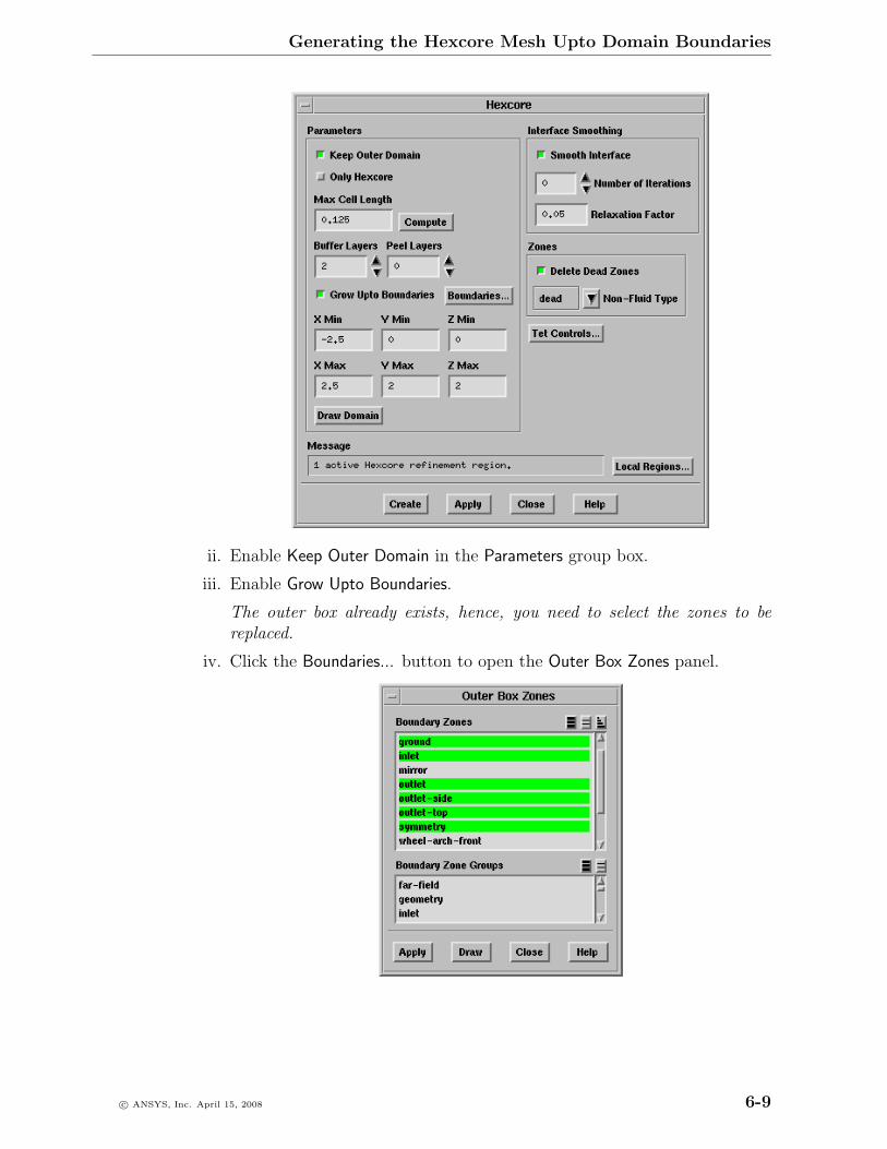
Generating the Hexcore Mesh Upto Domain Boundaries
ii. Enable Keep Outer Domain in the Parameters group box.
iii. Enable Grow Upto Boundaries.
The outer box already exists, hence, you need to select the zones to bereplaced.
iv. Click the Boundaries... button to open the Outer Box Zones panel.
c© ANSYS, Inc. April 15, 2008 6-9

Generating the Hexcore Mesh Upto Domain Boundaries
A. Select ground, inlet, outlet, outlet-side, outlet-top, and symmetry in theBoundary Zones selection list.
B. Click Apply and close the Outer Box Zones panel.
The domain extents will automatically be set to the size of the boundingbox. Make sure the domain extents are as follows:
X Min -2.5, Y Min 0, Z Min 0
X Max 2.5, Y Max 2, Z Max 2
v. Click Draw Domain to check the size of the domain to be meshed.
vi. Enter 0.125 for Max Cell Length.
vii. Set Buffer Layers to 2.
Setting the number of buffer layers to 2 ensures smoother size variation.
viii. Set Peel Layers to 0.
The peel layer controls the gap between the hexahedra core and the ge-ometry. The lower the peel layer specified, the fewer the tetrahedral cellsgenerated.
ix. Enable Delete Dead Zones in the Zones group box.
x. Click the Tet Controls... button to open the Tri/Tet panel.
A. Retain the default settings in the Initialization tab.
B. Click the Refinement tab and retain the selection of geometric in theCell Size Function drop-down list.
C. Enter 1.3 for Growth Rate and click Apply.
D. Close the Tri/Tet panel.
xi. Define the local refinement region.
A. Click the Local Regions... button to open the Hexcore Refinement Re-gion panel.
6-10 c© ANSYS, Inc. April 15, 2008
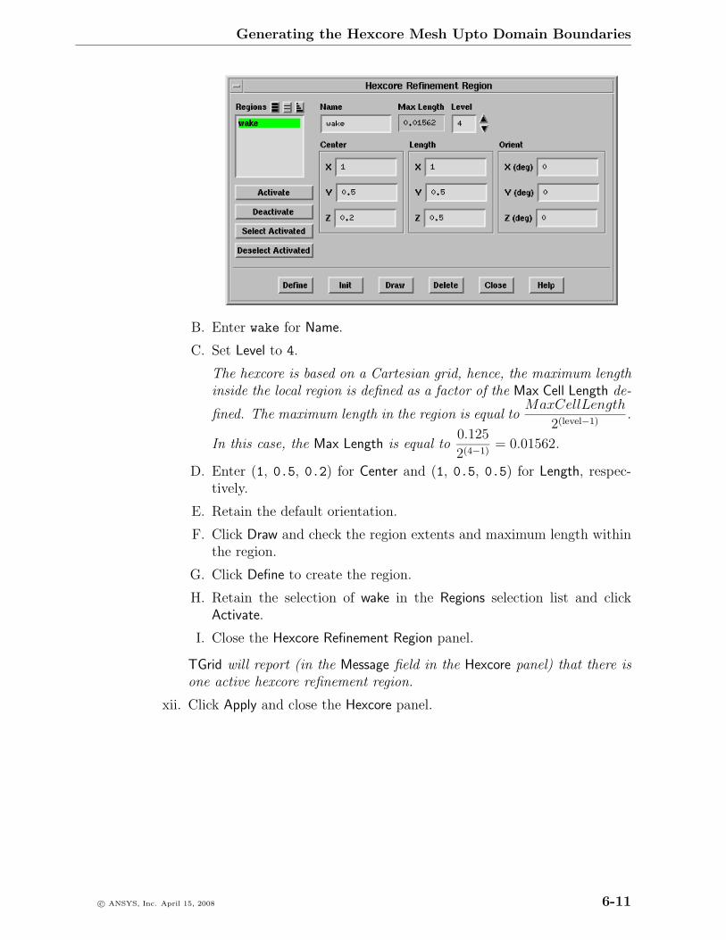
Generating the Hexcore Mesh Upto Domain Boundaries
B. Enter wake for Name.
C. Set Level to 4.
The hexcore is based on a Cartesian grid, hence, the maximum lengthinside the local region is defined as a factor of the Max Cell Length de-
fined. The maximum length in the region is equal toMaxCellLength
2(level−1).
In this case, the Max Length is equal to0.125
2(4−1)= 0.01562.
D. Enter (1, 0.5, 0.2) for Center and (1, 0.5, 0.5) for Length, respec-tively.
E. Retain the default orientation.
F. Click Draw and check the region extents and maximum length withinthe region.
G. Click Define to create the region.
H. Retain the selection of wake in the Regions selection list and clickActivate.
I. Close the Hexcore Refinement Region panel.
TGrid will report (in the Message field in the Hexcore panel) that there isone active hexcore refinement region.
xii. Click Apply and close the Hexcore panel.
c© ANSYS, Inc. April 15, 2008 6-11
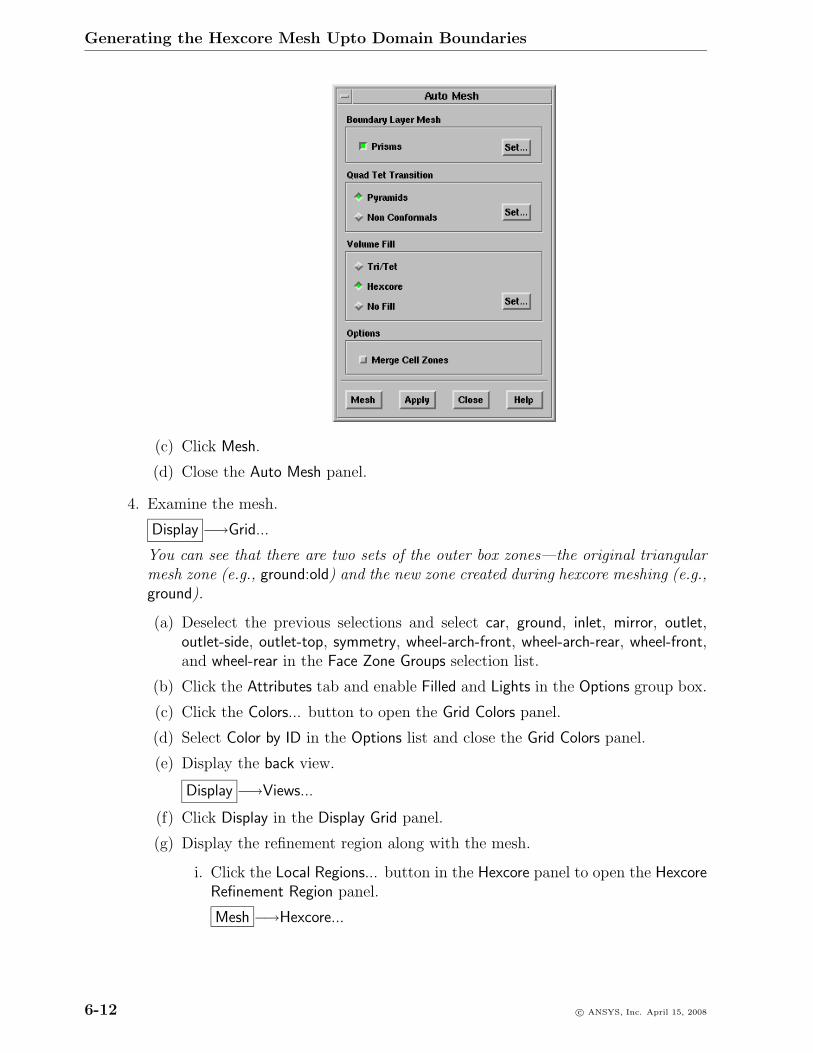
Generating the Hexcore Mesh Upto Domain Boundaries
(c) Click Mesh.
(d) Close the Auto Mesh panel.
4. Examine the mesh.
Display −→Grid...
You can see that there are two sets of the outer box zones—the original triangularmesh zone (e.g., ground:old) and the new zone created during hexcore meshing (e.g.,ground).
(a) Deselect the previous selections and select car, ground, inlet, mirror, outlet,outlet-side, outlet-top, symmetry, wheel-arch-front, wheel-arch-rear, wheel-front,and wheel-rear in the Face Zone Groups selection list.
(b) Click the Attributes tab and enable Filled and Lights in the Options group box.
(c) Click the Colors... button to open the Grid Colors panel.
(d) Select Color by ID in the Options list and close the Grid Colors panel.
(e) Display the back view.
Display −→Views...
(f) Click Display in the Display Grid panel.
(g) Display the refinement region along with the mesh.
i. Click the Local Regions... button in the Hexcore panel to open the HexcoreRefinement Region panel.
Mesh −→Hexcore...
6-12 c© ANSYS, Inc. April 15, 2008
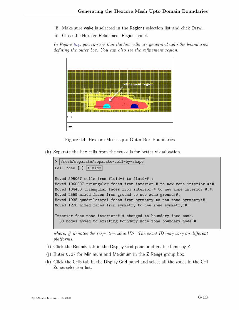
Generating the Hexcore Mesh Upto Domain Boundaries
ii. Make sure wake is selected in the Regions selection list and click Draw.
iii. Close the Hexcore Refinement Region panel.
In Figure 6.4, you can see that the hex cells are generated upto the boundariesdefining the outer box. You can also see the refinement region.
Figure 6.4: Hexcore Mesh Upto Outer Box Boundaries
(h) Separate the hex cells from the tet cells for better visualization.
> /mesh/separate/separate-cell-by-shape
Cell Zone [ ] fluid*
Moved 595067 cells from fluid-# to fluid-#:#Moved 1060007 triangular faces from interior-# to new zone interior-#:#.Moved 134450 triangular faces from interior-# to new zone interior-#:#.Moved 2559 mixed faces from ground to new zone ground:#.Moved 1935 quadrilateral faces from symmetry to new zone symmetry:#.Moved 1270 mixed faces from symmetry to new zone symmetry:#.
Interior face zone interior-#:# changed to boundary face zone.38 nodes moved to existing boundary node zone boundary-node-#
where, # denotes the respective zone IDs. The exact ID may vary on differentplatforms.
(i) Click the Bounds tab in the Display Grid panel and enable Limit by Z.
(j) Enter 0.37 for Minimum and Maximum in the Z Range group box.
(k) Click the Cells tab in the Display Grid panel and select all the zones in the CellZones selection list.
c© ANSYS, Inc. April 15, 2008 6-13
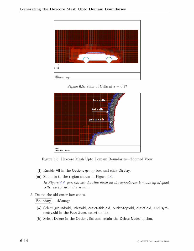
Generating the Hexcore Mesh Upto Domain Boundaries
Figure 6.5: Slide of Cells at z = 0.37
Figure 6.6: Hexcore Mesh Upto Domain Boundaries—Zoomed View
(l) Enable All in the Options group box and click Display.
(m) Zoom in to the region shown in Figure 6.6.
In Figure 6.6, you can see that the mesh on the boundaries is made up of quadcells, except near the sedan.
5. Delete the old outer box zones.
Boundary −→Manage...
(a) Select ground:old, inlet:old, outlet-side:old, outlet-top:old, outlet:old, and sym-metry:old in the Face Zones selection list.
(b) Select Delete in the Options list and retain the Delete Nodes option.
6-14 c© ANSYS, Inc. April 15, 2008

Generating the Hexcore Mesh Upto Domain Boundaries
(c) Click Apply.
A Question dialog will appear, asking you to confirm if you want to delete theselected zones.
(d) Click Yes in the Question dialog box.
(e) Close the Manage Face Zones panel.
6. Check the mesh.
Mesh −→Check
7. Save the mesh file.
File −→ Write −→Mesh...
8. Exit TGrid.
File −→Exit
Summary
This tutorial demonstrated the generation of a hexcore mesh upto the domain boundariesfor a sedan car. It also demonstrated the creation of prism layers and the use of localrefinement regions in conjunction with the hexcore mesh generation.
c© ANSYS, Inc. April 15, 2008 6-15

Generating the Hexcore Mesh Upto Domain Boundaries
6-16 c© ANSYS, Inc. April 15, 2008
Tutorial 7. Using the Boundary Wrapper
Introduction
Geometries imported from various CAD packages often contain gaps and/or overlapsbetween surfaces. Repairing such geometries manually is a tedious and time-consumingprocess. The boundary wrapper in TGrid can be used to repair such geometries auto-matically, thereby reducing the time required for preprocessing.
The wrapping procedure is based on the Cartesian grid (or overlay grid) approach. Ini-tially, a coarse Cartesian grid is overlaid on the input geometry and the intersectionbetween the Cartesian grid and the geometry is calculated. The intersecting cells areidentified and a watertight faceted representation is created along the boundary of thesecells. The nodes on the faceted representation are projected onto the input geometryresulting in a wrapper surface that closely resembles the input geometry.
This tutorial demonstrates how to do the following:
1. Read and display the mesh.
2. Perform pre-wrapping operations to close holes in the geometry.
3. Initialize the wrapper.
4. Check the region to be wrapped.
5. Refine the Cartesian grid using the local size function.
6. Wrap the surface and imprint necessary features.
7. Check the deviation of the wrapper surface from the original geometry.
8. Perform post-wrapping operations to improve wrapper surface quality.
9. Check and save the mesh.
The V-8 engine geometry used in this tutorial is provided by Platinum Pictures Multi-media Inc., www.3dcafe.com, and Michael Barthels.
Prerequisites
This tutorial assumes that you have some experience with TGrid, and that you are familiarwith the graphical user interface.
c© ANSYS, Inc. April 15, 2008 7-1
Using the Boundary Wrapper
Preparation
1. Download wrapper.zip from the FLUENT User Services Center
This file can be found from the Documentation link on the TGrid product page.
OR
Copy wrapper.zip from the TGrid documentation CD to your working directory.
• For UNIX systems, insert the CD into your CD-ROM drive and go to thefollowing directory:
cdrom/tgrid5.0/help/tutfiles/
where, cdrom must be replaced by the name of your CD-ROM drive.
• For Windows systems, insert the CD into your CD-ROM drive and go to thefollowing folder:
cdrom:\tgrid5.0\help\tutfiles\
where, cdrom must be replaced by the name of your CD-ROM drive (e.g., E).
2. Unzip wrapper.zip.
The files v8-airintake out.msh, v8-block out.msh, v8-cylinder-left out.msh,v8-cylinder-right out.msh, v8-generator out.msh, v8-manfold out.msh,v8-top-left out.msh, v8-top-right out.msh, and v8-wheels out.msh can befound in the v8 folder created on unzipping the file.
3. Start the 3D (3d) version of TGrid.
7-2 c© ANSYS, Inc. April 15, 2008
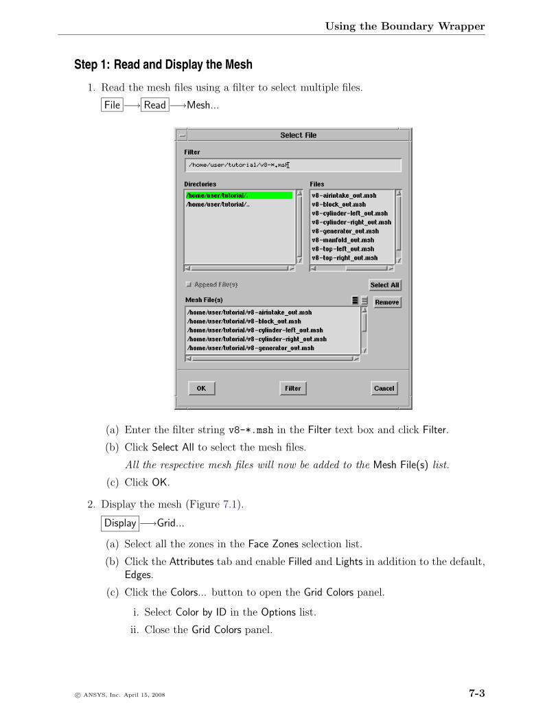
Using the Boundary Wrapper
Step 1: Read and Display the Mesh
1. Read the mesh files using a filter to select multiple files.
File −→ Read −→Mesh...
(a) Enter the filter string v8-*.msh in the Filter text box and click Filter.
(b) Click Select All to select the mesh files.
All the respective mesh files will now be added to the Mesh File(s) list.
(c) Click OK.
2. Display the mesh (Figure 7.1).
Display −→Grid...
(a) Select all the zones in the Face Zones selection list.
(b) Click the Attributes tab and enable Filled and Lights in addition to the default,Edges.
(c) Click the Colors... button to open the Grid Colors panel.
i. Select Color by ID in the Options list.
ii. Close the Grid Colors panel.
c© ANSYS, Inc. April 15, 2008 7-3
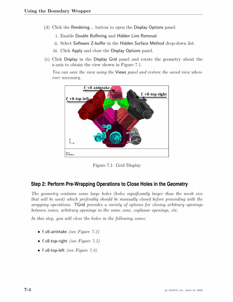
Using the Boundary Wrapper
(d) Click the Rendering... button to open the Display Options panel.
i. Enable Double Buffering and Hidden Line Removal.
ii. Select Software Z-buffer in the Hidden Surface Method drop-down list.
iii. Click Apply and close the Display Options panel.
(e) Click Display in the Display Grid panel and rotate the geometry about thex-axis to obtain the view shown in Figure 7.1.
You can save the view using the Views panel and restore the saved view when-ever necessary.
Figure 7.1: Grid Display
Step 2: Perform Pre-Wrapping Operations to Close Holes in the Geometry
The geometry contains some large holes (holes significantly larger than the mesh sizethat will be used) which preferably should be manually closed before proceeding with thewrapping operations. TGrid provides a variety of options for closing arbitrary openingsbetween zones, arbitrary openings in the same zone, coplanar openings, etc.
In this step, you will close the holes in the following zones:
• f v8-airintake (see Figure 7.2)
• f v8-top-right (see Figure 7.5)
• f v8-top-left (see Figure 7.8)
7-4 c© ANSYS, Inc. April 15, 2008
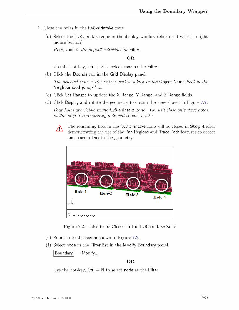
Using the Boundary Wrapper
1. Close the holes in the f v8-airintake zone.
(a) Select the f v8-airintake zone in the display window (click on it with the rightmouse button).
Here, zone is the default selection for Filter.
OR
Use the hot-key, Ctrl + Z to select zone as the Filter.
(b) Click the Bounds tab in the Grid Display panel.
The selected zone, f v8-airintake will be added in the Object Name field in theNeighborhood group box.
(c) Click Set Ranges to update the X Range, Y Range, and Z Range fields.
(d) Click Display and rotate the geometry to obtain the view shown in Figure 7.2.
Four holes are visible in the f v8-airintake zone. You will close only three holesin this step, the remaining hole will be closed later.
! The remaining hole in the f v8-airintake zone will be closed in Step 4 afterdemonstrating the use of the Pan Regions and Trace Path features to detectand trace a leak in the geometry.
Figure 7.2: Holes to be Closed in the f v8-airintake Zone
(e) Zoom in to the region shown in Figure 7.3.
(f) Select node in the Filter list in the Modify Boundary panel.
Boundary −→Modify...
OR
Use the hot-key, Ctrl + N to select node as the Filter.
c© ANSYS, Inc. April 15, 2008 7-5
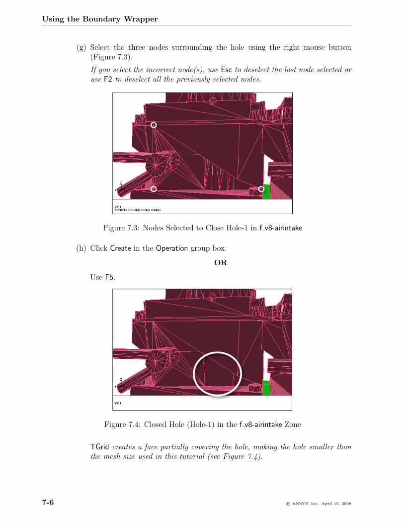
Using the Boundary Wrapper
(g) Select the three nodes surrounding the hole using the right mouse button(Figure 7.3).
If you select the incorrect node(s), use Esc to deselect the last node selected oruse F2 to deselect all the previously selected nodes.
Figure 7.3: Nodes Selected to Close Hole-1 in f v8-airintake
(h) Click Create in the Operation group box.
OR
Use F5.
Figure 7.4: Closed Hole (Hole-1) in the f v8-airintake Zone
TGrid creates a face partially covering the hole, making the hole smaller thanthe mesh size used in this tutorial (see Figure 7.4).
7-6 c© ANSYS, Inc. April 15, 2008
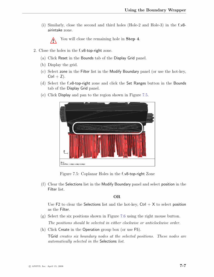
Using the Boundary Wrapper
(i) Similarly, close the second and third holes (Hole-2 and Hole-3) in the f v8-airintake zone.
! You will close the remaining hole in Step 4.
2. Close the holes in the f v8-top-right zone.
(a) Click Reset in the Bounds tab of the Display Grid panel.
(b) Display the grid.
(c) Select zone in the Filter list in the Modify Boundary panel (or use the hot-key,Ctrl + Z).
(d) Select the f v8-top-right zone and click the Set Ranges button in the Boundstab of the Display Grid panel.
(e) Click Display and pan to the region shown in Figure 7.5.
Figure 7.5: Coplanar Holes in the f v8-top-right Zone
(f) Clear the Selections list in the Modify Boundary panel and select position in theFilter list.
OR
Use F2 to clear the Selections list and the hot-key, Ctrl + X to select positionas the Filter.
(g) Select the six positions shown in Figure 7.6 using the right mouse button.
The positions should be selected in either clockwise or anticlockwise order.
(h) Click Create in the Operation group box (or use F5).
TGrid creates six boundary nodes at the selected positions. These nodes areautomatically selected in the Selections list.
c© ANSYS, Inc. April 15, 2008 7-7
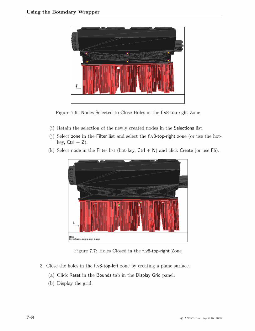
Using the Boundary Wrapper
Figure 7.6: Nodes Selected to Close Holes in the f v8-top-right Zone
(i) Retain the selection of the newly created nodes in the Selections list.
(j) Select zone in the Filter list and select the f v8-top-right zone (or use the hot-key, Ctrl + Z).
(k) Select node in the Filter list (hot-key, Ctrl + N) and click Create (or use F5).
Figure 7.7: Holes Closed in the f v8-top-right Zone
3. Close the holes in the f v8-top-left zone by creating a plane surface.
(a) Click Reset in the Bounds tab in the Display Grid panel.
(b) Display the grid.
7-8 c© ANSYS, Inc. April 15, 2008
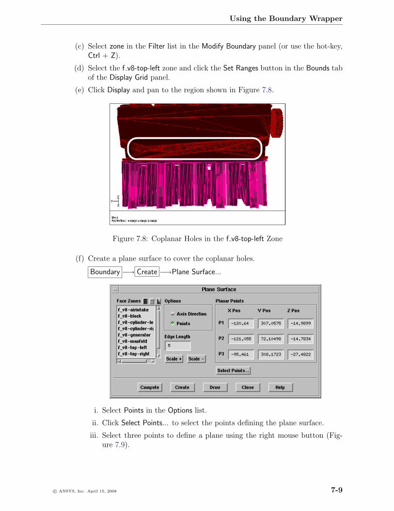
Using the Boundary Wrapper
(c) Select zone in the Filter list in the Modify Boundary panel (or use the hot-key,Ctrl + Z).
(d) Select the f v8-top-left zone and click the Set Ranges button in the Bounds tabof the Display Grid panel.
(e) Click Display and pan to the region shown in Figure 7.8.
Figure 7.8: Coplanar Holes in the f v8-top-left Zone
(f) Create a plane surface to cover the coplanar holes.
Boundary −→ Create −→Plane Surface...
i. Select Points in the Options list.
ii. Click Select Points... to select the points defining the plane surface.
iii. Select three points to define a plane using the right mouse button (Fig-ure 7.9).
c© ANSYS, Inc. April 15, 2008 7-9
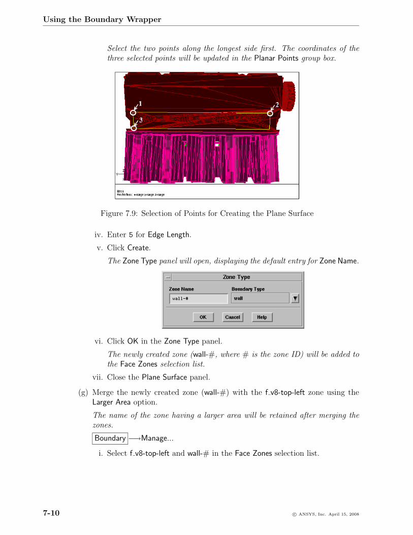
Using the Boundary Wrapper
Select the two points along the longest side first. The coordinates of thethree selected points will be updated in the Planar Points group box.
Figure 7.9: Selection of Points for Creating the Plane Surface
iv. Enter 5 for Edge Length.
v. Click Create.
The Zone Type panel will open, displaying the default entry for Zone Name.
vi. Click OK in the Zone Type panel.
The newly created zone (wall-#, where # is the zone ID) will be added tothe Face Zones selection list.
vii. Close the Plane Surface panel.
(g) Merge the newly created zone (wall-#) with the f v8-top-left zone using theLarger Area option.
The name of the zone having a larger area will be retained after merging thezones.
Boundary −→Manage...
i. Select f v8-top-left and wall-# in the Face Zones selection list.
7-10 c© ANSYS, Inc. April 15, 2008
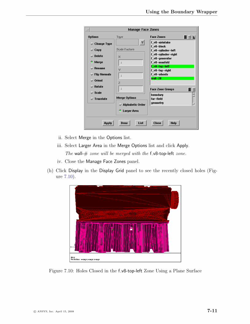
Using the Boundary Wrapper
ii. Select Merge in the Options list.
iii. Select Larger Area in the Merge Options list and click Apply.
The wall-# zone will be merged with the f v8-top-left zone.
iv. Close the Manage Face Zones panel.
(h) Click Display in the Display Grid panel to see the recently closed holes (Fig-ure 7.10).
Figure 7.10: Holes Closed in the f v8-top-left Zone Using a Plane Surface
c© ANSYS, Inc. April 15, 2008 7-11
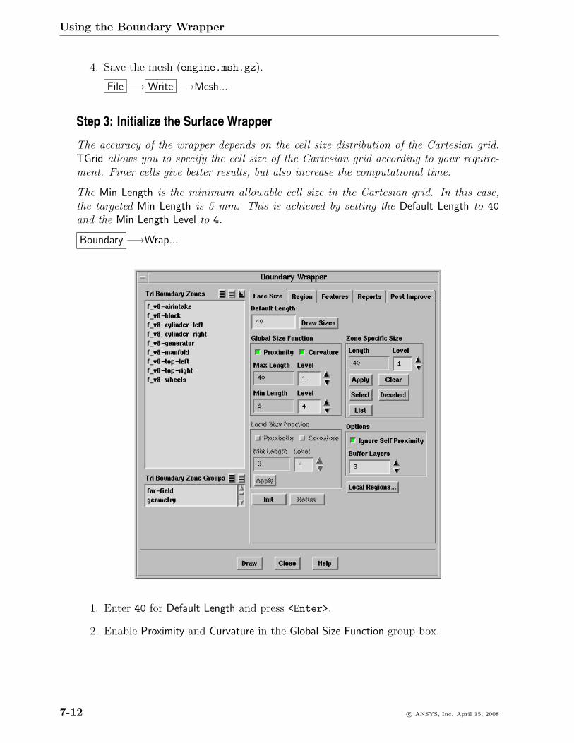
Using the Boundary Wrapper
4. Save the mesh (engine.msh.gz).
File −→ Write −→Mesh...
Step 3: Initialize the Surface Wrapper
The accuracy of the wrapper depends on the cell size distribution of the Cartesian grid.TGrid allows you to specify the cell size of the Cartesian grid according to your require-ment. Finer cells give better results, but also increase the computational time.
The Min Length is the minimum allowable cell size in the Cartesian grid. In this case,the targeted Min Length is 5 mm. This is achieved by setting the Default Length to 40
and the Min Length Level to 4.
Boundary −→Wrap...
1. Enter 40 for Default Length and press <Enter>.
2. Enable Proximity and Curvature in the Global Size Function group box.
7-12 c© ANSYS, Inc. April 15, 2008
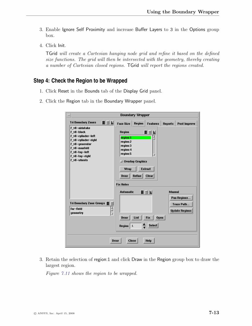
Using the Boundary Wrapper
3. Enable Ignore Self Proximity and increase Buffer Layers to 3 in the Options groupbox.
4. Click Init.
TGrid will create a Cartesian hanging node grid and refine it based on the definedsize functions. The grid will then be intersected with the geometry, thereby creatinga number of Cartesian closed regions. TGrid will report the regions created.
Step 4: Check the Region to be Wrapped
1. Click Reset in the Bounds tab of the Display Grid panel.
2. Click the Region tab in the Boundary Wrapper panel.
3. Retain the selection of region:1 and click Draw in the Region group box to draw thelargest region.
Figure 7.11 shows the region to be wrapped.
c© ANSYS, Inc. April 15, 2008 7-13
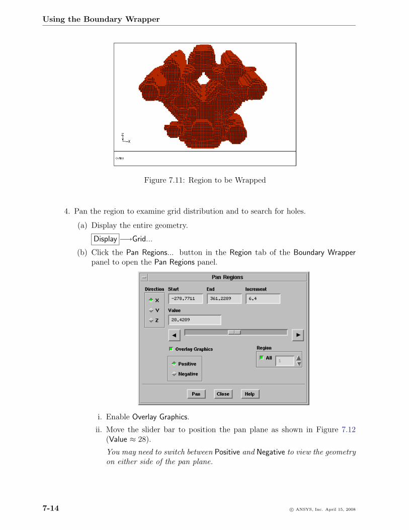
Using the Boundary Wrapper
Figure 7.11: Region to be Wrapped
4. Pan the region to examine grid distribution and to search for holes.
(a) Display the entire geometry.
Display −→Grid...
(b) Click the Pan Regions... button in the Region tab of the Boundary Wrapperpanel to open the Pan Regions panel.
i. Enable Overlay Graphics.
ii. Move the slider bar to position the pan plane as shown in Figure 7.12(Value ≈ 28).
You may need to switch between Positive and Negative to view the geometryon either side of the pan plane.
7-14 c© ANSYS, Inc. April 15, 2008
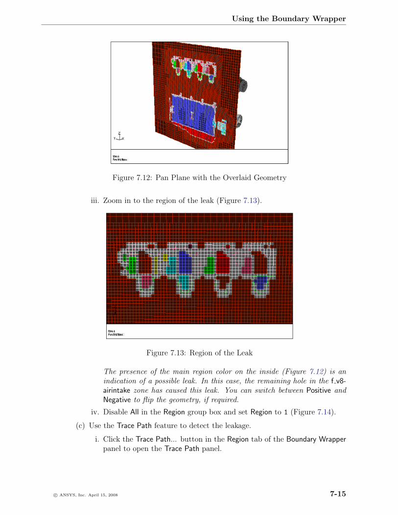
Using the Boundary Wrapper
Figure 7.12: Pan Plane with the Overlaid Geometry
iii. Zoom in to the region of the leak (Figure 7.13).
Figure 7.13: Region of the Leak
The presence of the main region color on the inside (Figure 7.12) is anindication of a possible leak. In this case, the remaining hole in the f v8-airintake zone has caused this leak. You can switch between Positive andNegative to flip the geometry, if required.
iv. Disable All in the Region group box and set Region to 1 (Figure 7.14).
(c) Use the Trace Path feature to detect the leakage.
i. Click the Trace Path... button in the Region tab of the Boundary Wrapperpanel to open the Trace Path panel.
c© ANSYS, Inc. April 15, 2008 7-15
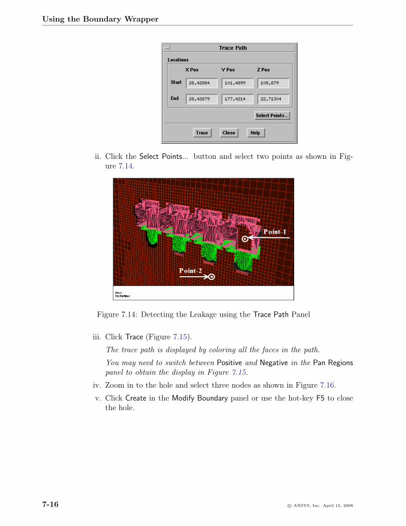
Using the Boundary Wrapper
ii. Click the Select Points... button and select two points as shown in Fig-ure 7.14.
Figure 7.14: Detecting the Leakage using the Trace Path Panel
iii. Click Trace (Figure 7.15).
The trace path is displayed by coloring all the faces in the path.
You may need to switch between Positive and Negative in the Pan Regionspanel to obtain the display in Figure 7.15.
iv. Zoom in to the hole and select three nodes as shown in Figure 7.16.
v. Click Create in the Modify Boundary panel or use the hot-key F5 to closethe hole.
7-16 c© ANSYS, Inc. April 15, 2008
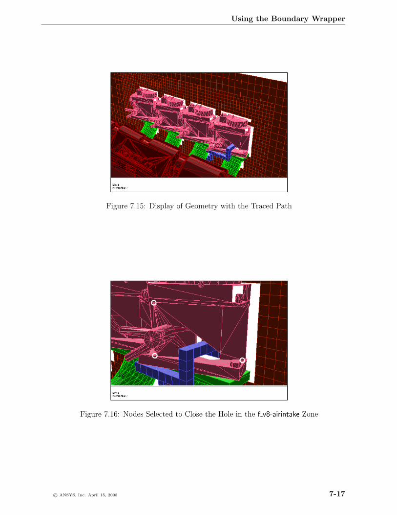
Using the Boundary Wrapper
Figure 7.15: Display of Geometry with the Traced Path
Figure 7.16: Nodes Selected to Close the Hole in the f v8-airintake Zone
c© ANSYS, Inc. April 15, 2008 7-17
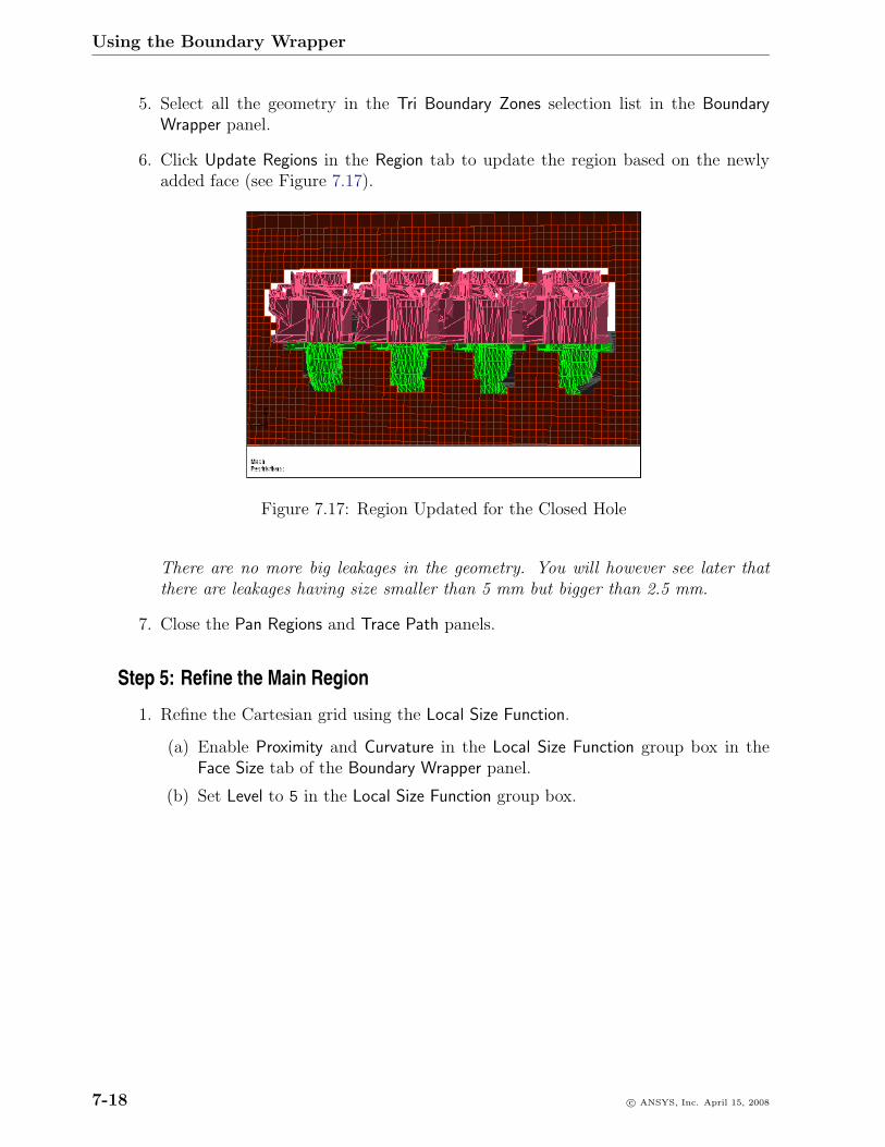
Using the Boundary Wrapper
5. Select all the geometry in the Tri Boundary Zones selection list in the BoundaryWrapper panel.
6. Click Update Regions in the Region tab to update the region based on the newlyadded face (see Figure 7.17).
Figure 7.17: Region Updated for the Closed Hole
There are no more big leakages in the geometry. You will however see later thatthere are leakages having size smaller than 5 mm but bigger than 2.5 mm.
7. Close the Pan Regions and Trace Path panels.
Step 5: Refine the Main Region
1. Refine the Cartesian grid using the Local Size Function.
(a) Enable Proximity and Curvature in the Local Size Function group box in theFace Size tab of the Boundary Wrapper panel.
(b) Set Level to 5 in the Local Size Function group box.
7-18 c© ANSYS, Inc. April 15, 2008
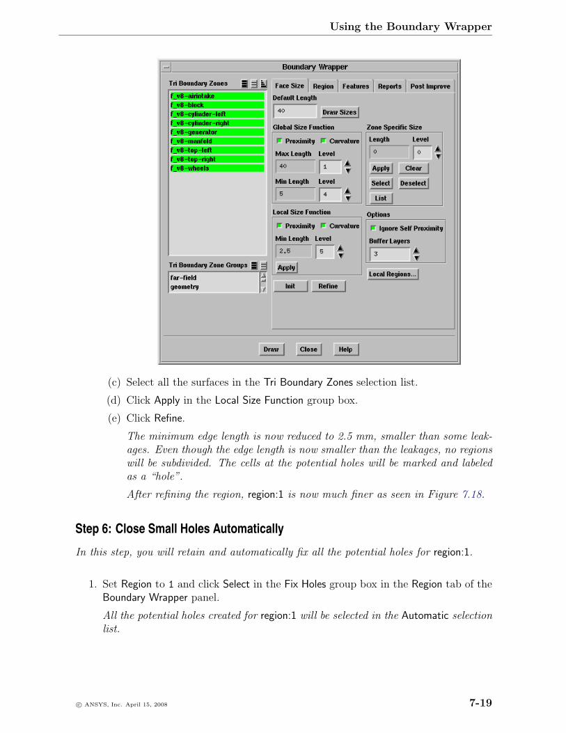
Using the Boundary Wrapper
(c) Select all the surfaces in the Tri Boundary Zones selection list.
(d) Click Apply in the Local Size Function group box.
(e) Click Refine.
The minimum edge length is now reduced to 2.5 mm, smaller than some leak-ages. Even though the edge length is now smaller than the leakages, no regionswill be subdivided. The cells at the potential holes will be marked and labeledas a “hole”.
After refining the region, region:1 is now much finer as seen in Figure 7.18.
Step 6: Close Small Holes Automatically
In this step, you will retain and automatically fix all the potential holes for region:1.
1. Set Region to 1 and click Select in the Fix Holes group box in the Region tab of theBoundary Wrapper panel.
All the potential holes created for region:1 will be selected in the Automatic selectionlist.
c© ANSYS, Inc. April 15, 2008 7-19
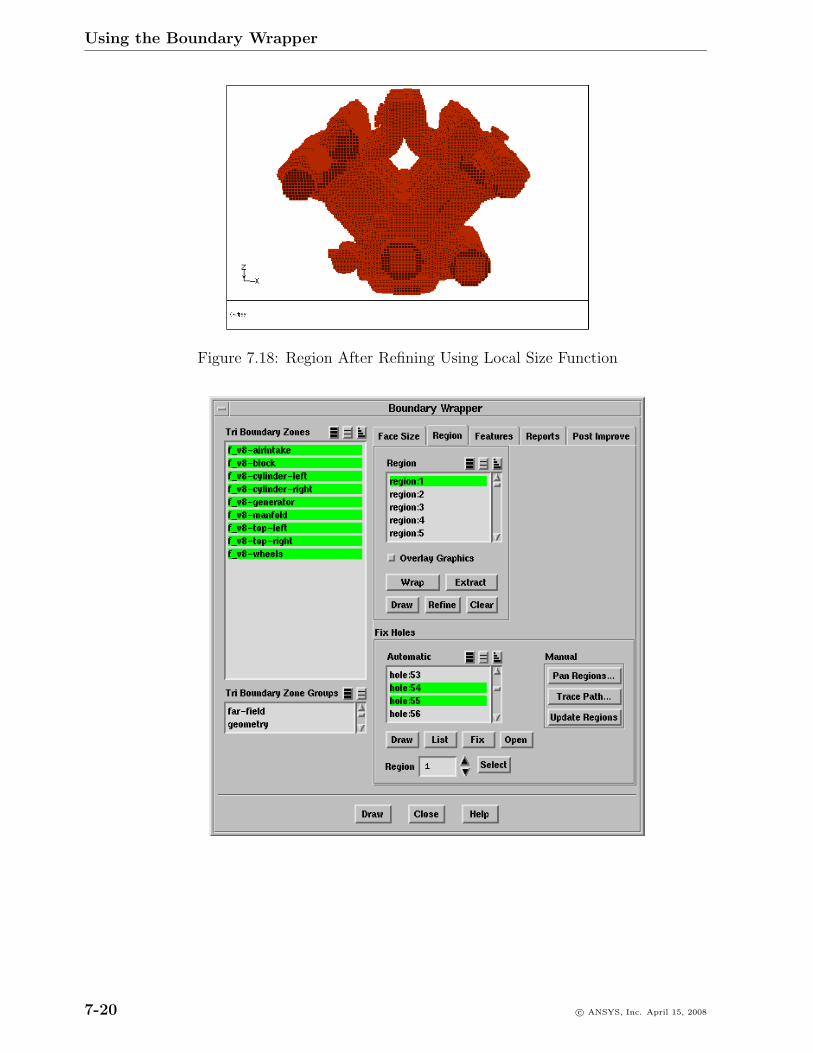
Using the Boundary Wrapper
Figure 7.18: Region After Refining Using Local Size Function
7-20 c© ANSYS, Inc. April 15, 2008
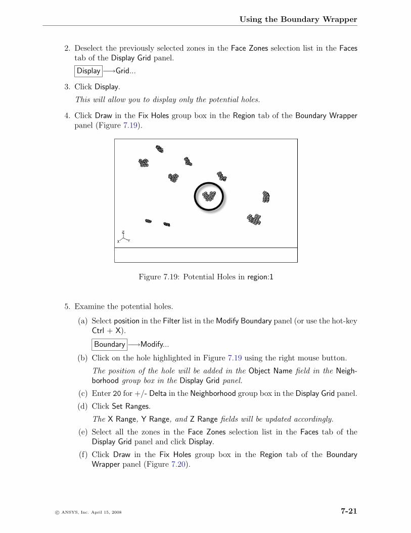
Using the Boundary Wrapper
2. Deselect the previously selected zones in the Face Zones selection list in the Facestab of the Display Grid panel.
Display −→Grid...
3. Click Display.
This will allow you to display only the potential holes.
4. Click Draw in the Fix Holes group box in the Region tab of the Boundary Wrapperpanel (Figure 7.19).
Figure 7.19: Potential Holes in region:1
5. Examine the potential holes.
(a) Select position in the Filter list in the Modify Boundary panel (or use the hot-keyCtrl + X).
Boundary −→Modify...
(b) Click on the hole highlighted in Figure 7.19 using the right mouse button.
The position of the hole will be added in the Object Name field in the Neigh-borhood group box in the Display Grid panel.
(c) Enter 20 for +/- Delta in the Neighborhood group box in the Display Grid panel.
(d) Click Set Ranges.
The X Range, Y Range, and Z Range fields will be updated accordingly.
(e) Select all the zones in the Face Zones selection list in the Faces tab of theDisplay Grid panel and click Display.
(f) Click Draw in the Fix Holes group box in the Region tab of the BoundaryWrapper panel (Figure 7.20).
c© ANSYS, Inc. April 15, 2008 7-21
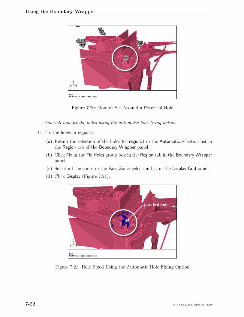
Using the Boundary Wrapper
Figure 7.20: Bounds Set Around a Potential Hole
You will now fix the holes using the automatic hole fixing option.
6. Fix the holes in region:1.
(a) Retain the selection of the holes for region:1 in the Automatic selection list inthe Region tab of the Boundary Wrapper panel.
(b) Click Fix in the Fix Holes group box in the Region tab in the Boundary Wrapperpanel.
(c) Select all the zones in the Face Zones selection list in the Display Grid panel.
(d) Click Display (Figure 7.21).
Figure 7.21: Hole Fixed Using the Automatic Hole Fixing Option
7-22 c© ANSYS, Inc. April 15, 2008
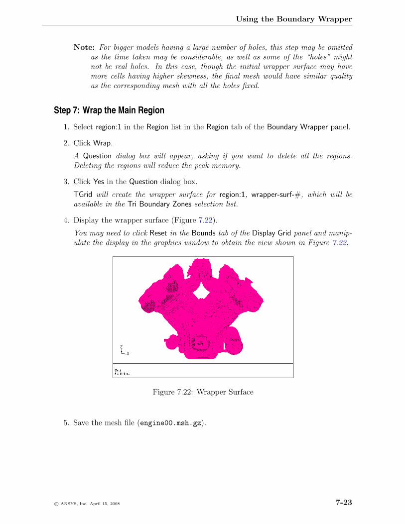
Using the Boundary Wrapper
Note: For bigger models having a large number of holes, this step may be omittedas the time taken may be considerable, as well as some of the “holes” mightnot be real holes. In this case, though the initial wrapper surface may havemore cells having higher skewness, the final mesh would have similar qualityas the corresponding mesh with all the holes fixed.
Step 7: Wrap the Main Region
1. Select region:1 in the Region list in the Region tab of the Boundary Wrapper panel.
2. Click Wrap.
A Question dialog box will appear, asking if you want to delete all the regions.Deleting the regions will reduce the peak memory.
3. Click Yes in the Question dialog box.
TGrid will create the wrapper surface for region:1, wrapper-surf-#, which will beavailable in the Tri Boundary Zones selection list.
4. Display the wrapper surface (Figure 7.22).
You may need to click Reset in the Bounds tab of the Display Grid panel and manip-ulate the display in the graphics window to obtain the view shown in Figure 7.22.
Figure 7.22: Wrapper Surface
5. Save the mesh file (engine00.msh.gz).
c© ANSYS, Inc. April 15, 2008 7-23
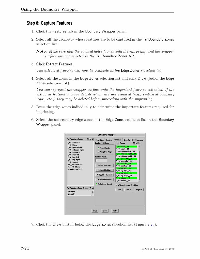
Using the Boundary Wrapper
Step 8: Capture Features
1. Click the Features tab in the Boundary Wrapper panel.
2. Select all the geometry whose features are to be captured in the Tri Boundary Zonesselection list.
Note: Make sure that the patched holes (zones with the vs prefix) and the wrappersurface are not selected in the Tri Boundary Zones list.
3. Click Extract Features.
The extracted features will now be available in the Edge Zones selection list.
4. Select all the zones in the Edge Zones selection list and click Draw (below the EdgeZones selection list).
You can reproject the wrapper surface onto the important features extracted. If theextracted features include details which are not required (e.g., embossed companylogos, etc.), they may be deleted before proceeding with the imprinting.
5. Draw the edge zones individually to determine the important features required forimprinting.
6. Select the unnecessary edge zones in the Edge Zones selection list in the BoundaryWrapper panel.
7. Click the Draw button below the Edge Zones selection list (Figure 7.23).
7-24 c© ANSYS, Inc. April 15, 2008
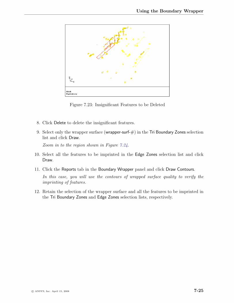
Using the Boundary Wrapper
Figure 7.23: Insignificant Features to be Deleted
8. Click Delete to delete the insignificant features.
9. Select only the wrapper surface (wrapper-surf-#) in the Tri Boundary Zones selectionlist and click Draw.
Zoom in to the region shown in Figure 7.24.
10. Select all the features to be imprinted in the Edge Zones selection list and clickDraw.
11. Click the Reports tab in the Boundary Wrapper panel and click Draw Contours.
In this case, you will use the contours of wrapped surface quality to verify theimprinting of features.
12. Retain the selection of the wrapper surface and all the features to be imprinted inthe Tri Boundary Zones and Edge Zones selection lists, respectively.
c© ANSYS, Inc. April 15, 2008 7-25
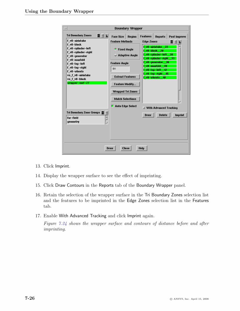
Using the Boundary Wrapper
13. Click Imprint.
14. Display the wrapper surface to see the effect of imprinting.
15. Click Draw Contours in the Reports tab of the Boundary Wrapper panel.
16. Retain the selection of the wrapper surface in the Tri Boundary Zones selection listand the features to be imprinted in the Edge Zones selection list in the Featurestab.
17. Enable With Advanced Tracking and click Imprint again.
Figure 7.24 shows the wrapper surface and contours of distance before and afterimprinting.
7-26 c© ANSYS, Inc. April 15, 2008
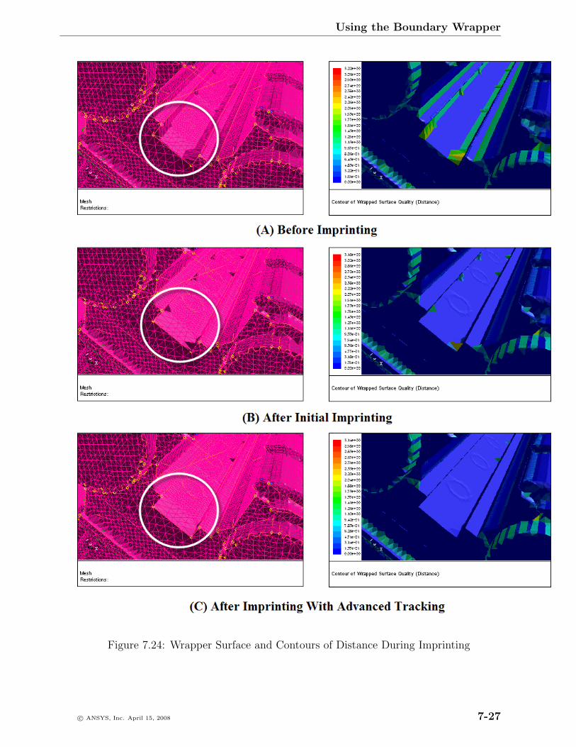
Using the Boundary Wrapper
Figure 7.24: Wrapper Surface and Contours of Distance During Imprinting
c© ANSYS, Inc. April 15, 2008 7-27
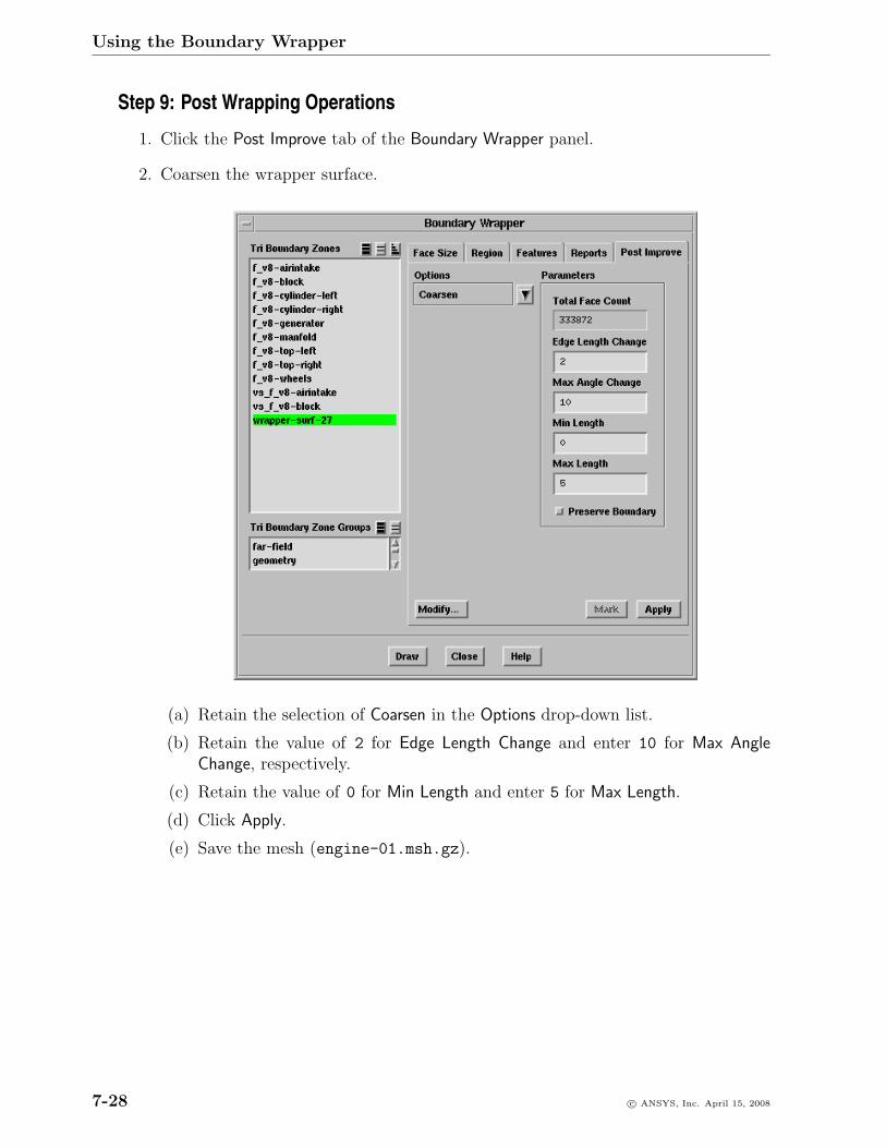
Using the Boundary Wrapper
Step 9: Post Wrapping Operations
1. Click the Post Improve tab of the Boundary Wrapper panel.
2. Coarsen the wrapper surface.
(a) Retain the selection of Coarsen in the Options drop-down list.
(b) Retain the value of 2 for Edge Length Change and enter 10 for Max AngleChange, respectively.
(c) Retain the value of 0 for Min Length and enter 5 for Max Length.
(d) Click Apply.
(e) Save the mesh (engine-01.msh.gz).
7-28 c© ANSYS, Inc. April 15, 2008
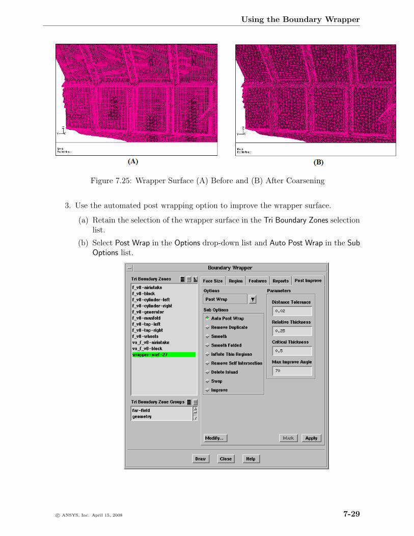
Using the Boundary Wrapper
Figure 7.25: Wrapper Surface (A) Before and (B) After Coarsening
3. Use the automated post wrapping option to improve the wrapper surface.
(a) Retain the selection of the wrapper surface in the Tri Boundary Zones selectionlist.
(b) Select Post Wrap in the Options drop-down list and Auto Post Wrap in the SubOptions list.
c© ANSYS, Inc. April 15, 2008 7-29
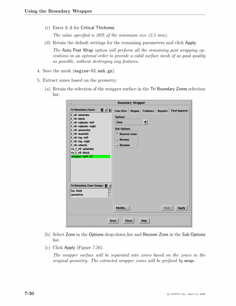
Using the Boundary Wrapper
(c) Enter 0.5 for Critical Thickness.
The value specified is 20% of the minimum size (2.5 mm).
(d) Retain the default settings for the remaining parameters and click Apply.
The Auto Post Wrap option will perform all the remaining post wrapping op-erations in an optimal order to provide a valid surface mesh of as good qualityas possible, without destroying any features.
4. Save the mesh (engine-02.msh.gz).
5. Extract zones based on the geometry.
(a) Retain the selection of the wrapper surface in the Tri Boundary Zones selectionlist.
(b) Select Zone in the Options drop-down list and Recover Zone in the Sub Optionslist.
(c) Click Apply (Figure 7.26).
The wrapper surface will be separated into zones based on the zones in theoriginal geometry. The extracted wrapper zones will be prefixed by wrap-.
7-30 c© ANSYS, Inc. April 15, 2008
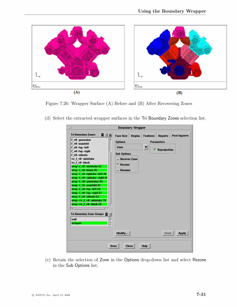
Using the Boundary Wrapper
Figure 7.26: Wrapper Surface (A) Before and (B) After Recovering Zones
(d) Select the extracted wrapper surfaces in the Tri Boundary Zones selection list.
(e) Retain the selection of Zone in the Options drop-down list and select Rezonein the Sub Options list.
c© ANSYS, Inc. April 15, 2008 7-31
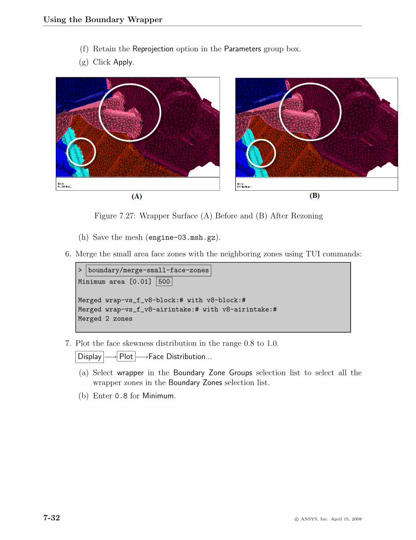
Using the Boundary Wrapper
(f) Retain the Reprojection option in the Parameters group box.
(g) Click Apply.
Figure 7.27: Wrapper Surface (A) Before and (B) After Rezoning
(h) Save the mesh (engine-03.msh.gz).
6. Merge the small area face zones with the neighboring zones using TUI commands:
> boundary/merge-small-face-zones
Minimum area [0.01] 500
Merged wrap-vs_f_v8-block:# with v8-block:#Merged wrap-vs_f_v8-airintake:# with v8-airintake:#Merged 2 zones
7. Plot the face skewness distribution in the range 0.8 to 1.0.
Display −→ Plot −→Face Distribution...
(a) Select wrapper in the Boundary Zone Groups selection list to select all thewrapper zones in the Boundary Zones selection list.
(b) Enter 0.8 for Minimum.
7-32 c© ANSYS, Inc. April 15, 2008
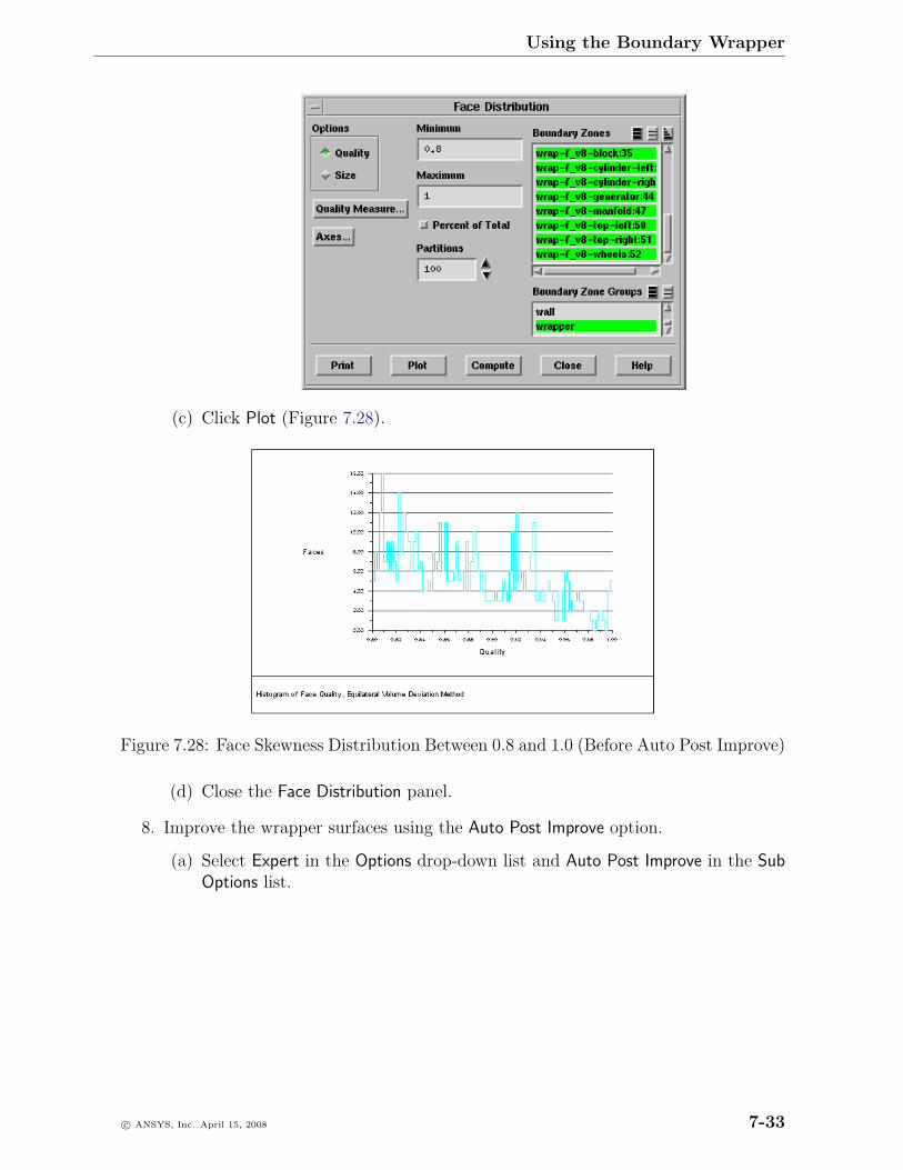
Using the Boundary Wrapper
(c) Click Plot (Figure 7.28).
Figure 7.28: Face Skewness Distribution Between 0.8 and 1.0 (Before Auto Post Improve)
(d) Close the Face Distribution panel.
8. Improve the wrapper surfaces using the Auto Post Improve option.
(a) Select Expert in the Options drop-down list and Auto Post Improve in the SubOptions list.
c© ANSYS, Inc. April 15, 2008 7-33
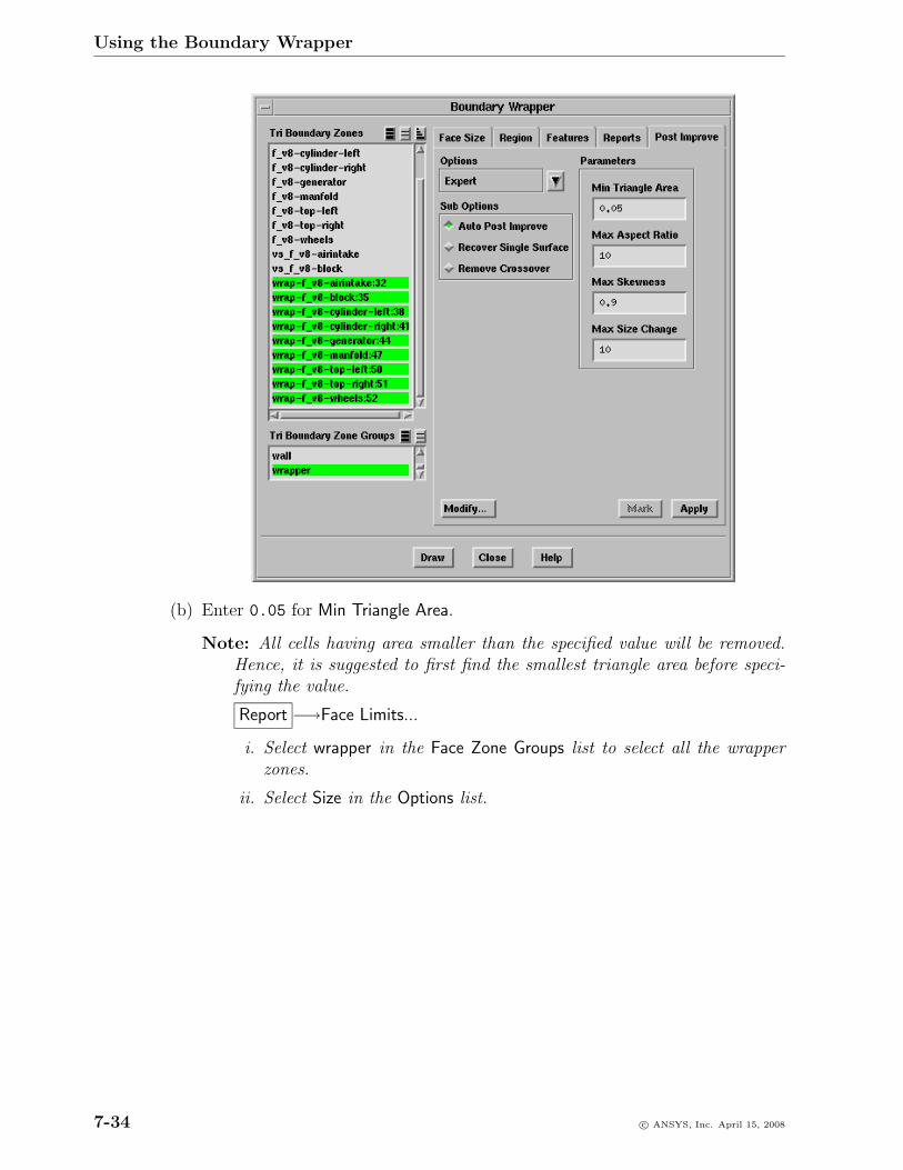
Using the Boundary Wrapper
(b) Enter 0.05 for Min Triangle Area.
Note: All cells having area smaller than the specified value will be removed.Hence, it is suggested to first find the smallest triangle area before speci-fying the value.
Report −→Face Limits...
i. Select wrapper in the Face Zone Groups list to select all the wrapperzones.
ii. Select Size in the Options list.
7-34 c© ANSYS, Inc. April 15, 2008
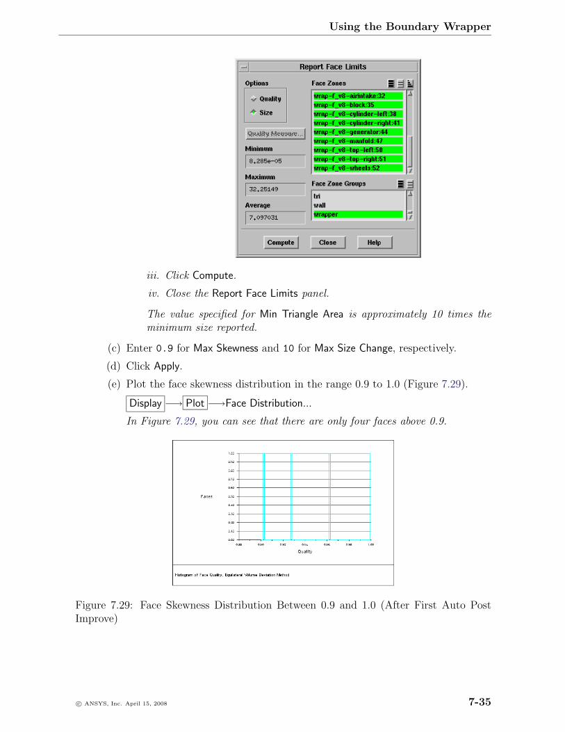
Using the Boundary Wrapper
iii. Click Compute.
iv. Close the Report Face Limits panel.
The value specified for Min Triangle Area is approximately 10 times theminimum size reported.
(c) Enter 0.9 for Max Skewness and 10 for Max Size Change, respectively.
(d) Click Apply.
(e) Plot the face skewness distribution in the range 0.9 to 1.0 (Figure 7.29).
Display −→ Plot −→Face Distribution...
In Figure 7.29, you can see that there are only four faces above 0.9.
Figure 7.29: Face Skewness Distribution Between 0.9 and 1.0 (After First Auto PostImprove)
c© ANSYS, Inc. April 15, 2008 7-35
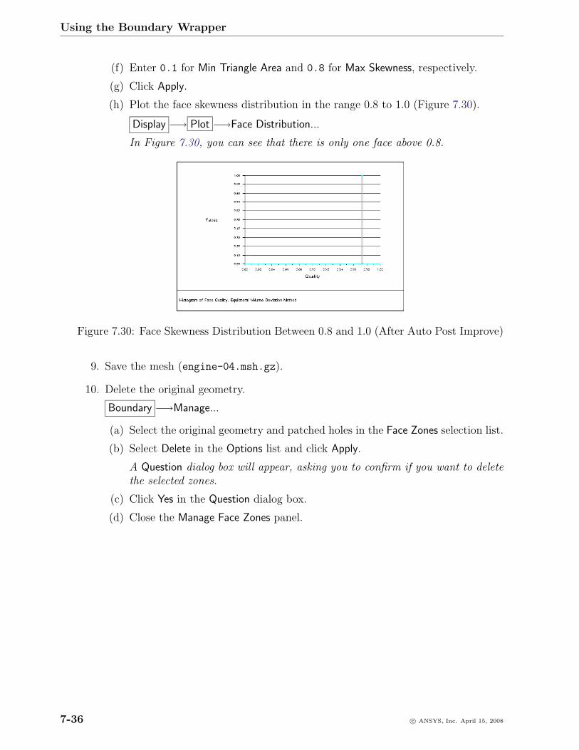
Using the Boundary Wrapper
(f) Enter 0.1 for Min Triangle Area and 0.8 for Max Skewness, respectively.
(g) Click Apply.
(h) Plot the face skewness distribution in the range 0.8 to 1.0 (Figure 7.30).
Display −→ Plot −→Face Distribution...
In Figure 7.30, you can see that there is only one face above 0.8.
Figure 7.30: Face Skewness Distribution Between 0.8 and 1.0 (After Auto Post Improve)
9. Save the mesh (engine-04.msh.gz).
10. Delete the original geometry.
Boundary −→Manage...
(a) Select the original geometry and patched holes in the Face Zones selection list.
(b) Select Delete in the Options list and click Apply.
A Question dialog box will appear, asking you to confirm if you want to deletethe selected zones.
(c) Click Yes in the Question dialog box.
(d) Close the Manage Face Zones panel.
7-36 c© ANSYS, Inc. April 15, 2008
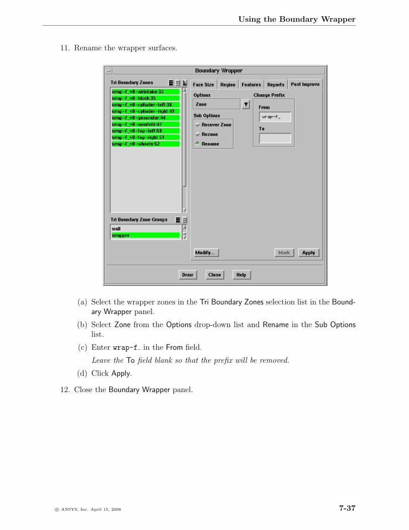
Using the Boundary Wrapper
11. Rename the wrapper surfaces.
(a) Select the wrapper zones in the Tri Boundary Zones selection list in the Bound-ary Wrapper panel.
(b) Select Zone from the Options drop-down list and Rename in the Sub Optionslist.
(c) Enter wrap-f in the From field.
Leave the To field blank so that the prefix will be removed.
(d) Click Apply.
12. Close the Boundary Wrapper panel.
c© ANSYS, Inc. April 15, 2008 7-37
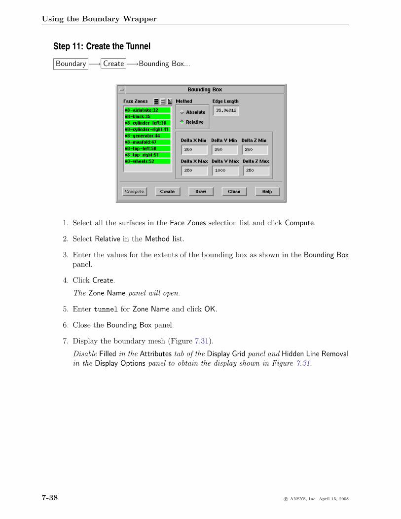
Using the Boundary Wrapper
Step 11: Create the Tunnel
Boundary −→ Create −→Bounding Box...
1. Select all the surfaces in the Face Zones selection list and click Compute.
2. Select Relative in the Method list.
3. Enter the values for the extents of the bounding box as shown in the Bounding Boxpanel.
4. Click Create.
The Zone Name panel will open.
5. Enter tunnel for Zone Name and click OK.
6. Close the Bounding Box panel.
7. Display the boundary mesh (Figure 7.31).
Disable Filled in the Attributes tab of the Display Grid panel and Hidden Line Removalin the Display Options panel to obtain the display shown in Figure 7.31.
7-38 c© ANSYS, Inc. April 15, 2008
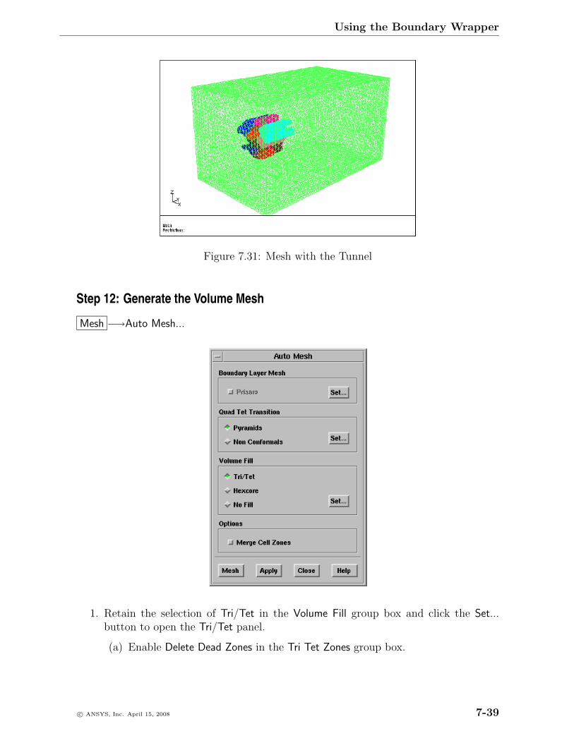
Using the Boundary Wrapper
Figure 7.31: Mesh with the Tunnel
Step 12: Generate the Volume Mesh
Mesh −→Auto Mesh...
1. Retain the selection of Tri/Tet in the Volume Fill group box and click the Set...button to open the Tri/Tet panel.
(a) Enable Delete Dead Zones in the Tri Tet Zones group box.
c© ANSYS, Inc. April 15, 2008 7-39
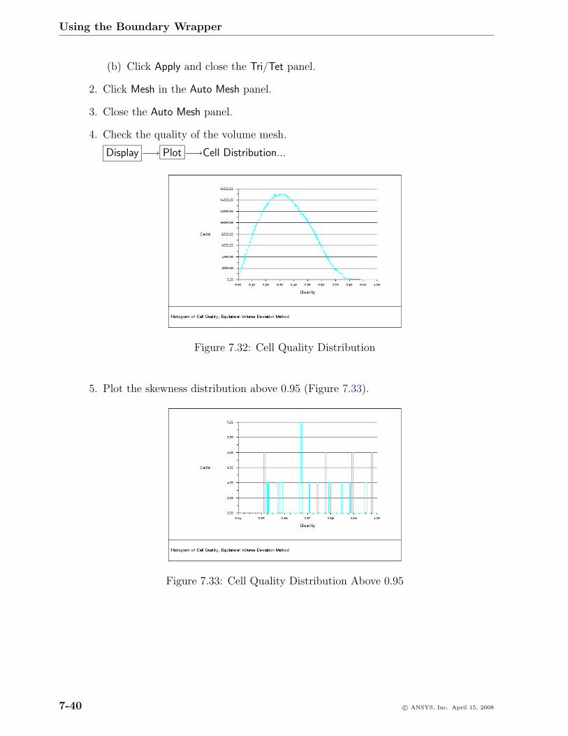
Using the Boundary Wrapper
(b) Click Apply and close the Tri/Tet panel.
2. Click Mesh in the Auto Mesh panel.
3. Close the Auto Mesh panel.
4. Check the quality of the volume mesh.
Display −→ Plot −→Cell Distribution...
Figure 7.32: Cell Quality Distribution
5. Plot the skewness distribution above 0.95 (Figure 7.33).
Figure 7.33: Cell Quality Distribution Above 0.95
7-40 c© ANSYS, Inc. April 15, 2008
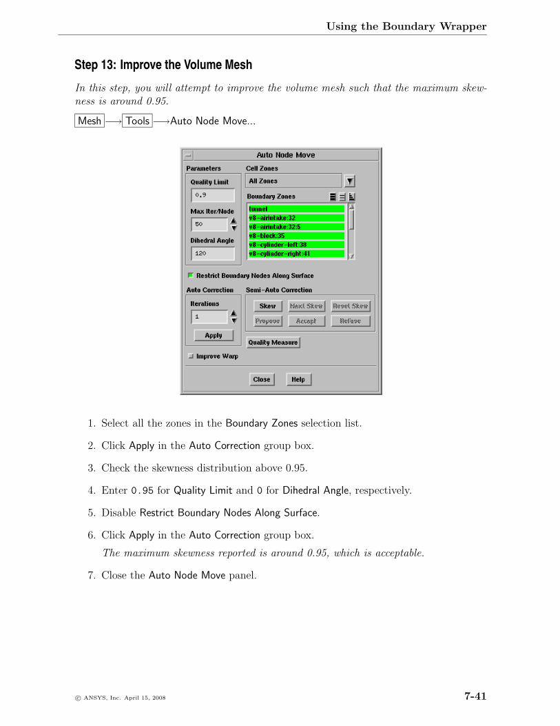
Using the Boundary Wrapper
Step 13: Improve the Volume Mesh
In this step, you will attempt to improve the volume mesh such that the maximum skew-ness is around 0.95.
Mesh −→ Tools −→Auto Node Move...
1. Select all the zones in the Boundary Zones selection list.
2. Click Apply in the Auto Correction group box.
3. Check the skewness distribution above 0.95.
4. Enter 0.95 for Quality Limit and 0 for Dihedral Angle, respectively.
5. Disable Restrict Boundary Nodes Along Surface.
6. Click Apply in the Auto Correction group box.
The maximum skewness reported is around 0.95, which is acceptable.
7. Close the Auto Node Move panel.
c© ANSYS, Inc. April 15, 2008 7-41
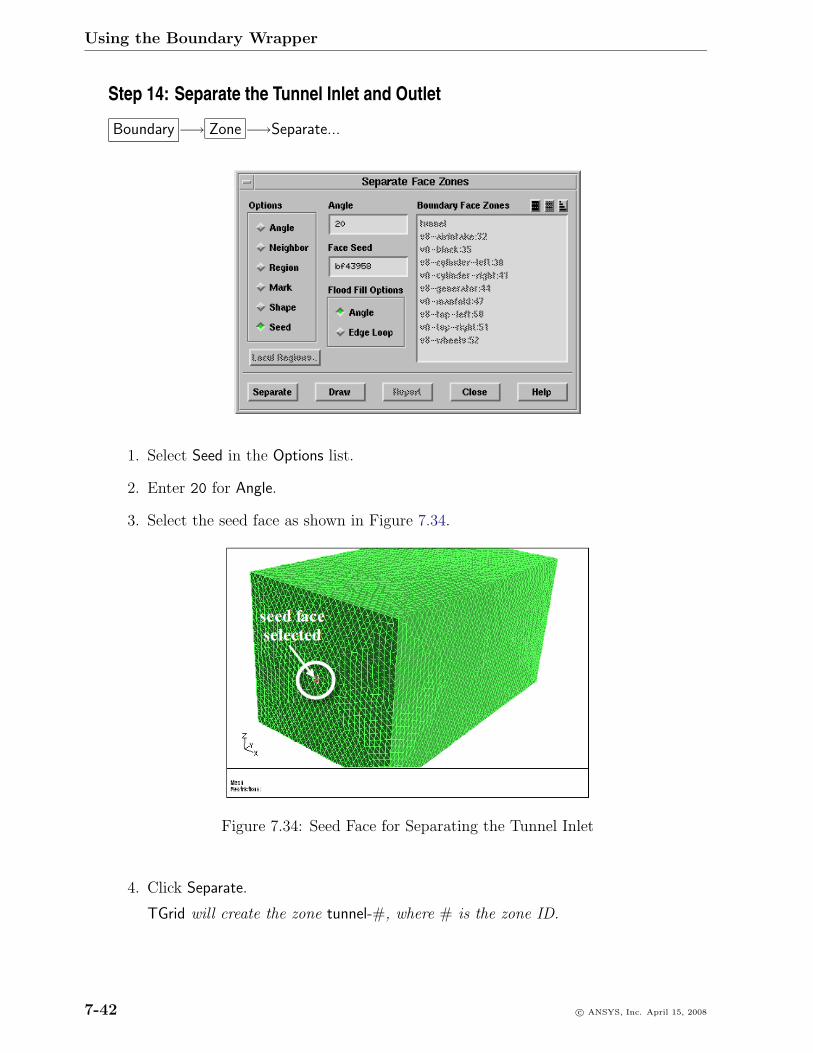
Using the Boundary Wrapper
Step 14: Separate the Tunnel Inlet and Outlet
Boundary −→ Zone −→Separate...
1. Select Seed in the Options list.
2. Enter 20 for Angle.
3. Select the seed face as shown in Figure 7.34.
Figure 7.34: Seed Face for Separating the Tunnel Inlet
4. Click Separate.
TGrid will create the zone tunnel-#, where # is the zone ID.
7-42 c© ANSYS, Inc. April 15, 2008
Using the Boundary Wrapper
5. Rename tunnel-# to inlet.
Boundary −→Manage...
(a) Select tunnel-# in the Face Zones selection list.
(b) Select Rename in the Options list.
(c) Enter inlet for Name and click Apply.
6. Similarly, separate the tunnel outlet and rename it to outlet.
7. Save the mesh (engine-final.msh.gz).
8. Exit TGrid.
Summary
This tutorial demonstrated the wrapping procedure for a V-8 engine mesh. You ini-tially performed pre-wrapping operations to close large holes in the geometry. You theninitialized the wrapper, examined the region to be wrapped and updated the region toaccount for the fixed leakage. The tutorial also demonstarted the use of the automatichole fixing functionality to close small holes detected when refining the Cartesian gridusing local size functions. After wrapping the main region, and imprinting necessary fea-tures of the geometry, you performed post-wrapping operations to improve the wrappersurface quality. You then created a tunnel encompassing the geometry and generated thevolume mesh. The tutorial also described the procedure for using the Auto Node Movefunctionality to improve the quality of the volume mesh.
c© ANSYS, Inc. April 15, 2008 7-43

Using the Boundary Wrapper
7-44 c© ANSYS, Inc. April 15, 2008
Tutorial 8. Cavity Remeshing
Introduction
Cavity remeshing is useful in parametric studies as it allows you to add, remove, orreplace different parts of an existing mesh. This tutorial demonstrates the procedure forreplacing an object in the existing mesh with another by creating a cavity and remeshingit. This tutorial demonstrates how to do the following:
1. Create and remesh a cavity to replace the mirror in a tetrahedral mesh.
2. Create and remesh a cavity in a hybrid mesh (tetrahedra and prisms) having asingle fluid zone.
3. Create and remesh a cavity in a hybrid mesh (tetrahedra and prisms) having mul-tiple fluid zones.
4. Create and remesh a cavity in a hexcore mesh.
Prerequisites
This tutorial assumes that you have some experience with TGrid, and that you are familiarwith the graphical user interface.
Preparation
1. Download cavity.zip from the FLUENT User Services Center to your workingdirectory. This file can be found from the Documentation link on the TGrid productpage.
OR
Copy cavity.zip from the TGrid documentation CD to your working directory.
• For UNIX systems, insert the CD into your CD-ROM drive and go to thefollowing directory:
cdrom/tgrid5.0/help/tutfiles
where, cdrom must be replaced by the name of your CD-ROM drive.
c© ANSYS, Inc. April 15, 2008 8-1

Cavity Remeshing
• For Windows systems, insert the CD into your CD-ROM drive and go to thefollowing folder:
cdrom:\tgrid5.0\help\tutfiles
where, cdrom must be replaced by the name of your CD-ROM drive (e.g., E).
2. Unzip cavity.zip.
The files, sedan tetra.msh.gz, sedan hyb-1zone.msh.gz, sedan hyb-2zones.msh.gz,sedan hexcore.msh.gz, mirror.msh.gz, and sedan hyb-2zones-cavity.jou canbe found in the cavity folder created on unzipping the file.
3. Start the 3D (3d) version of TGrid.
Case A. For a Tetrahedral Mesh
Step 1: Read and Display Mesh1. Read the mesh file.
File −→ Read −→Mesh...
(a) Select sedan tetra.msh.gz in the Files list.
(b) Click OK.
2. Examine the mesh.
Display −→Grid...
(a) Select car, mirror-old, wheel-arch-front, wheel-arch-rear, wheel-front, and wheel-rear, in the Face Zones selection list.
(b) Click Display (Figure 8.1).
(c) Click the Cells tab and enable All in the Options group box.
(d) Select fluid in the Cell Zone Groups selection list.
(e) Click the Bounds tab and enable Limit by X in the X Range group box.
(f) Enter -0.37 for both Minimum and Maximum in the X Range group box.
(g) Click Display.
8-2 c© ANSYS, Inc. April 15, 2008
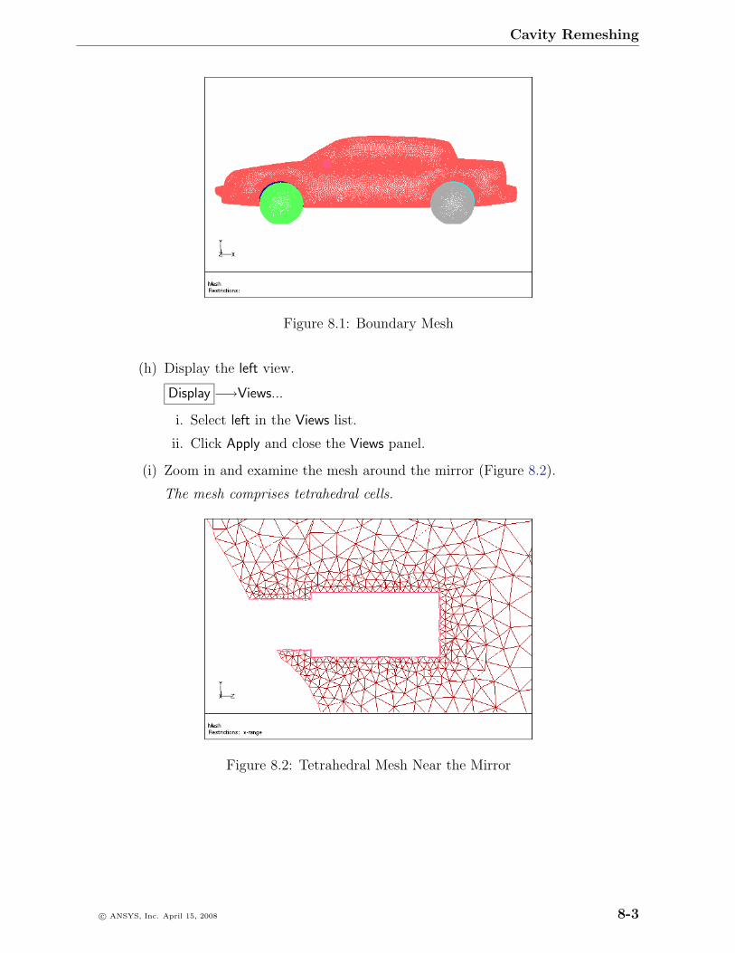
Cavity Remeshing
Figure 8.1: Boundary Mesh
(h) Display the left view.
Display −→Views...
i. Select left in the Views list.
ii. Click Apply and close the Views panel.
(i) Zoom in and examine the mesh around the mirror (Figure 8.2).
The mesh comprises tetrahedral cells.
Figure 8.2: Tetrahedral Mesh Near the Mirror
c© ANSYS, Inc. April 15, 2008 8-3
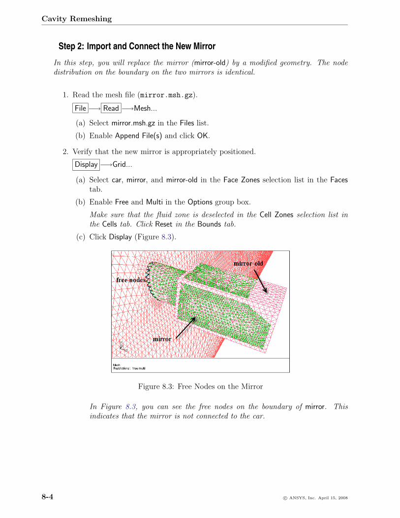
Cavity Remeshing
Step 2: Import and Connect the New Mirror
In this step, you will replace the mirror (mirror-old) by a modified geometry. The nodedistribution on the boundary on the two mirrors is identical.
1. Read the mesh file (mirror.msh.gz).
File −→ Read −→Mesh...
(a) Select mirror.msh.gz in the Files list.
(b) Enable Append File(s) and click OK.
2. Verify that the new mirror is appropriately positioned.
Display −→Grid...
(a) Select car, mirror, and mirror-old in the Face Zones selection list in the Facestab.
(b) Enable Free and Multi in the Options group box.
Make sure that the fluid zone is deselected in the Cell Zones selection list inthe Cells tab. Click Reset in the Bounds tab.
(c) Click Display (Figure 8.3).
Figure 8.3: Free Nodes on the Mirror
In Figure 8.3, you can see the free nodes on the boundary of mirror. Thisindicates that the mirror is not connected to the car.
8-4 c© ANSYS, Inc. April 15, 2008
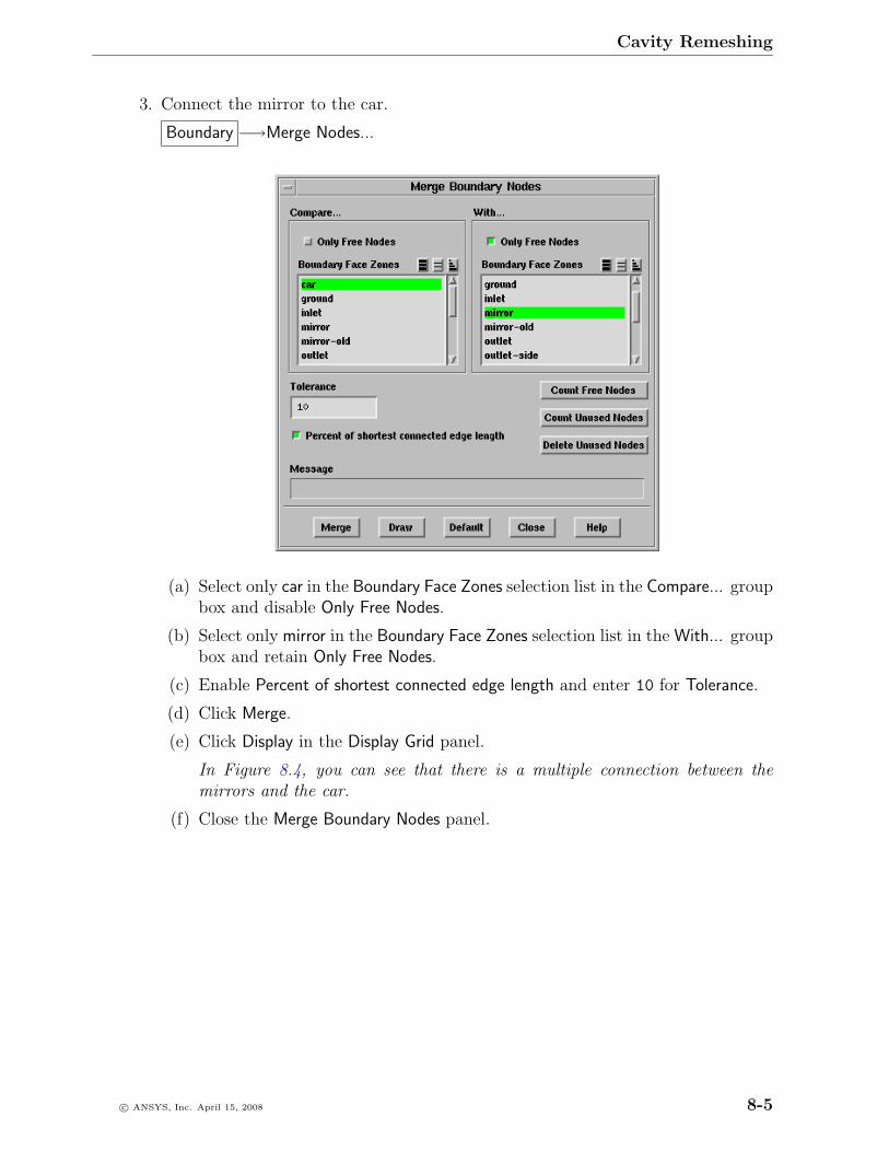
Cavity Remeshing
3. Connect the mirror to the car.
Boundary −→Merge Nodes...
(a) Select only car in the Boundary Face Zones selection list in the Compare... groupbox and disable Only Free Nodes.
(b) Select only mirror in the Boundary Face Zones selection list in the With... groupbox and retain Only Free Nodes.
(c) Enable Percent of shortest connected edge length and enter 10 for Tolerance.
(d) Click Merge.
(e) Click Display in the Display Grid panel.
In Figure 8.4, you can see that there is a multiple connection between themirrors and the car.
(f) Close the Merge Boundary Nodes panel.
c© ANSYS, Inc. April 15, 2008 8-5
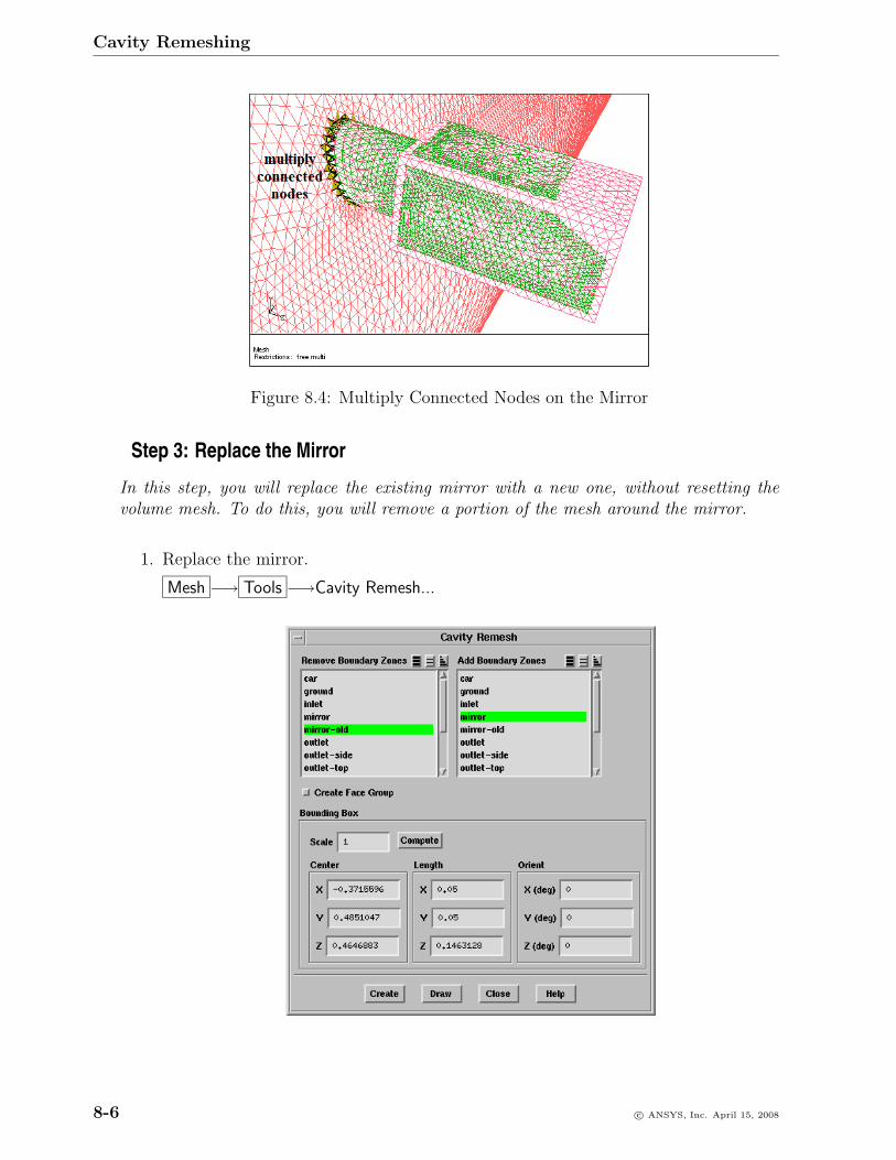
Cavity Remeshing
Figure 8.4: Multiply Connected Nodes on the Mirror
Step 3: Replace the Mirror
In this step, you will replace the existing mirror with a new one, without resetting thevolume mesh. To do this, you will remove a portion of the mesh around the mirror.
1. Replace the mirror.
Mesh −→ Tools −→Cavity Remesh...
8-6 c© ANSYS, Inc. April 15, 2008
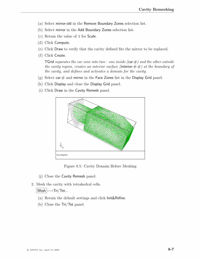
Cavity Remeshing
(a) Select mirror-old in the Remove Boundary Zones selection list.
(b) Select mirror in the Add Boundary Zones selection list.
(c) Retain the value of 1 for Scale.
(d) Click Compute.
(e) Click Draw to verify that the cavity defined fits the mirror to be replaced.
(f) Click Create.
TGrid separates the car zone into two—one inside (car:#) and the other outsidethe cavity region, creates an interior surface (interior-#:#) at the boundary ofthe cavity, and defines and activates a domain for the cavity.
(g) Select car:# and mirror in the Face Zones list in the Display Grid panel.
(h) Click Display and close the Display Grid panel.
(i) Click Draw in the Cavity Remesh panel.
Figure 8.5: Cavity Domain Before Meshing
(j) Close the Cavity Remesh panel.
2. Mesh the cavity with tetrahedral cells.
Mesh −→Tri/Tet...
(a) Retain the default settings and click Init&Refine.
(b) Close the Tri/Tet panel.
c© ANSYS, Inc. April 15, 2008 8-7
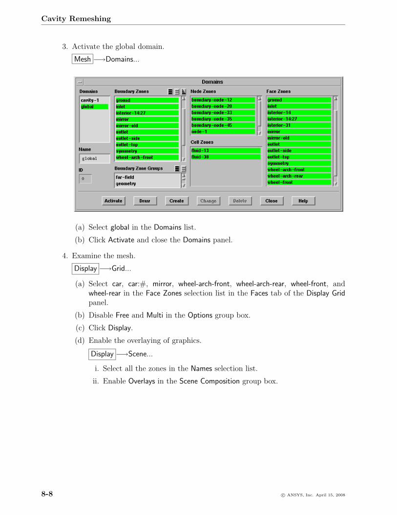
Cavity Remeshing
3. Activate the global domain.
Mesh −→Domains...
(a) Select global in the Domains list.
(b) Click Activate and close the Domains panel.
4. Examine the mesh.
Display −→Grid...
(a) Select car, car:#, mirror, wheel-arch-front, wheel-arch-rear, wheel-front, andwheel-rear in the Face Zones selection list in the Faces tab of the Display Gridpanel.
(b) Disable Free and Multi in the Options group box.
(c) Click Display.
(d) Enable the overlaying of graphics.
Display −→Scene...
i. Select all the zones in the Names selection list.
ii. Enable Overlays in the Scene Composition group box.
8-8 c© ANSYS, Inc. April 15, 2008
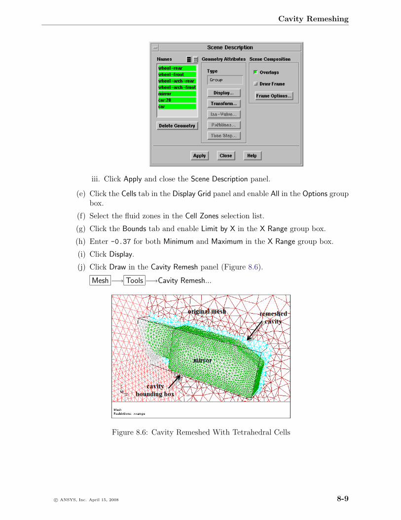
Cavity Remeshing
iii. Click Apply and close the Scene Description panel.
(e) Click the Cells tab in the Display Grid panel and enable All in the Options groupbox.
(f) Select the fluid zones in the Cell Zones selection list.
(g) Click the Bounds tab and enable Limit by X in the X Range group box.
(h) Enter -0.37 for both Minimum and Maximum in the X Range group box.
(i) Click Display.
(j) Click Draw in the Cavity Remesh panel (Figure 8.6).
Mesh −→ Tools −→Cavity Remesh...
Figure 8.6: Cavity Remeshed With Tetrahedral Cells
c© ANSYS, Inc. April 15, 2008 8-9
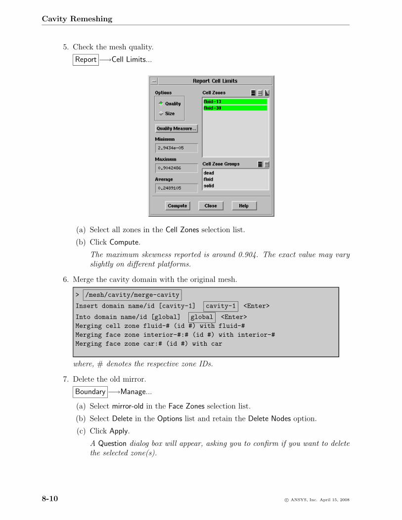
Cavity Remeshing
5. Check the mesh quality.
Report −→Cell Limits...
(a) Select all zones in the Cell Zones selection list.
(b) Click Compute.
The maximum skewness reported is around 0.904. The exact value may varyslightly on different platforms.
6. Merge the cavity domain with the original mesh.
> /mesh/cavity/merge-cavity
Insert domain name/id [cavity-1] cavity-1 <Enter>
Into domain name/id [global] global <Enter>Merging cell zone fluid-# (id #) with fluid-#Merging face zone interior-#:# (id #) with interior-#Merging face zone car:# (id #) with car
where, # denotes the respective zone IDs.
7. Delete the old mirror.
Boundary −→Manage...
(a) Select mirror-old in the Face Zones selection list.
(b) Select Delete in the Options list and retain the Delete Nodes option.
(c) Click Apply.
A Question dialog box will appear, asking you to confirm if you want to deletethe selected zone(s).
8-10 c© ANSYS, Inc. April 15, 2008

Cavity Remeshing
(d) Click Yes in the Question dialog box.
(e) Close the Manage Face Zones panel.
8. Check the mesh.
Mesh −→Check
9. Save the mesh (sedan-tet-cavity.msh.gz).
File −→ Write −→Mesh...
Case B. For a Hybrid Mesh (Tetrahedra and Prisms) Having a Single Fluid Zone
1. Read the mesh file (sedan hyb-1zone.msh.gz).
File −→ Read −→Mesh...
(a) Select sedan hyb-1zone.msh.gz in the Files list.
(b) Click OK.
2. Examine the mesh.
Display −→Grid...
(a) Click the Cells tab and enable All in the Options group box.
(b) Select fluid in the Cell Zone Groups selection list.
(c) Click the Bounds tab and enable Limit by X in the X Range group box.
(d) Enter -0.37 for both Minimum and Maximum in the X Range group box.
(e) Click Display.
(f) Display the left view.
Display −→Views...
(g) Zoom in and examine the mesh around the mirror (Figure 8.7).
3. Import and connect the mirror.
(a) Read the mesh file mirror.msh.gz with the Append File(s) option enabled.
File −→ Read −→Mesh...
c© ANSYS, Inc. April 15, 2008 8-11
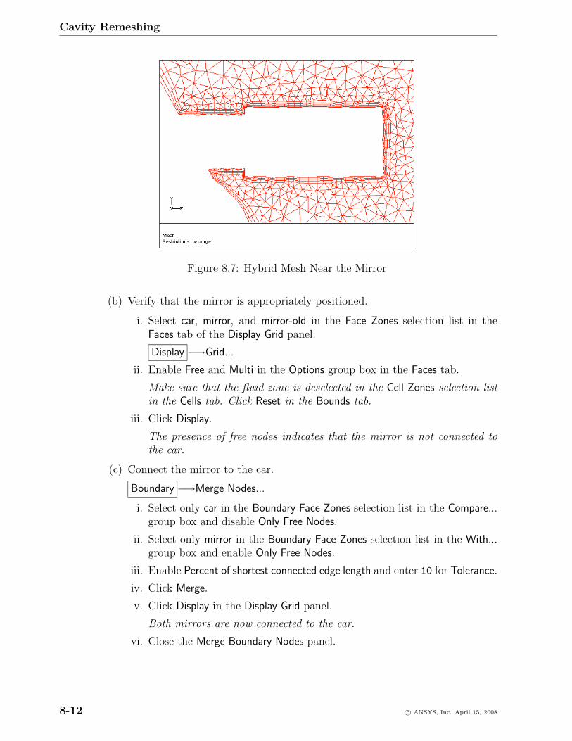
Cavity Remeshing
Figure 8.7: Hybrid Mesh Near the Mirror
(b) Verify that the mirror is appropriately positioned.
i. Select car, mirror, and mirror-old in the Face Zones selection list in theFaces tab of the Display Grid panel.
Display −→Grid...
ii. Enable Free and Multi in the Options group box in the Faces tab.
Make sure that the fluid zone is deselected in the Cell Zones selection listin the Cells tab. Click Reset in the Bounds tab.
iii. Click Display.
The presence of free nodes indicates that the mirror is not connected tothe car.
(c) Connect the mirror to the car.
Boundary −→Merge Nodes...
i. Select only car in the Boundary Face Zones selection list in the Compare...group box and disable Only Free Nodes.
ii. Select only mirror in the Boundary Face Zones selection list in the With...group box and enable Only Free Nodes.
iii. Enable Percent of shortest connected edge length and enter 10 for Tolerance.
iv. Click Merge.
v. Click Display in the Display Grid panel.
Both mirrors are now connected to the car.
vi. Close the Merge Boundary Nodes panel.
8-12 c© ANSYS, Inc. April 15, 2008
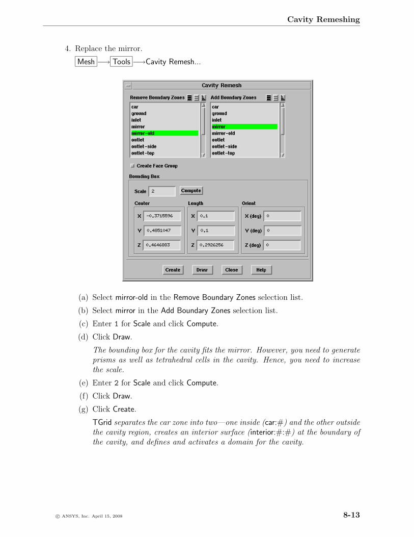
Cavity Remeshing
4. Replace the mirror.
Mesh −→ Tools −→Cavity Remesh...
(a) Select mirror-old in the Remove Boundary Zones selection list.
(b) Select mirror in the Add Boundary Zones selection list.
(c) Enter 1 for Scale and click Compute.
(d) Click Draw.
The bounding box for the cavity fits the mirror. However, you need to generateprisms as well as tetrahedral cells in the cavity. Hence, you need to increasethe scale.
(e) Enter 2 for Scale and click Compute.
(f) Click Draw.
(g) Click Create.
TGrid separates the car zone into two—one inside (car:#) and the other outsidethe cavity region, creates an interior surface (interior:#:#) at the boundary ofthe cavity, and defines and activates a domain for the cavity.
c© ANSYS, Inc. April 15, 2008 8-13
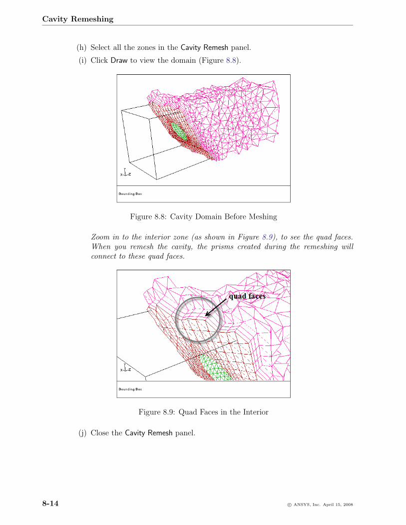
Cavity Remeshing
(h) Select all the zones in the Cavity Remesh panel.
(i) Click Draw to view the domain (Figure 8.8).
Figure 8.8: Cavity Domain Before Meshing
Zoom in to the interior zone (as shown in Figure 8.9), to see the quad faces.When you remesh the cavity, the prisms created during the remeshing willconnect to these quad faces.
Figure 8.9: Quad Faces in the Interior
(j) Close the Cavity Remesh panel.
8-14 c© ANSYS, Inc. April 15, 2008
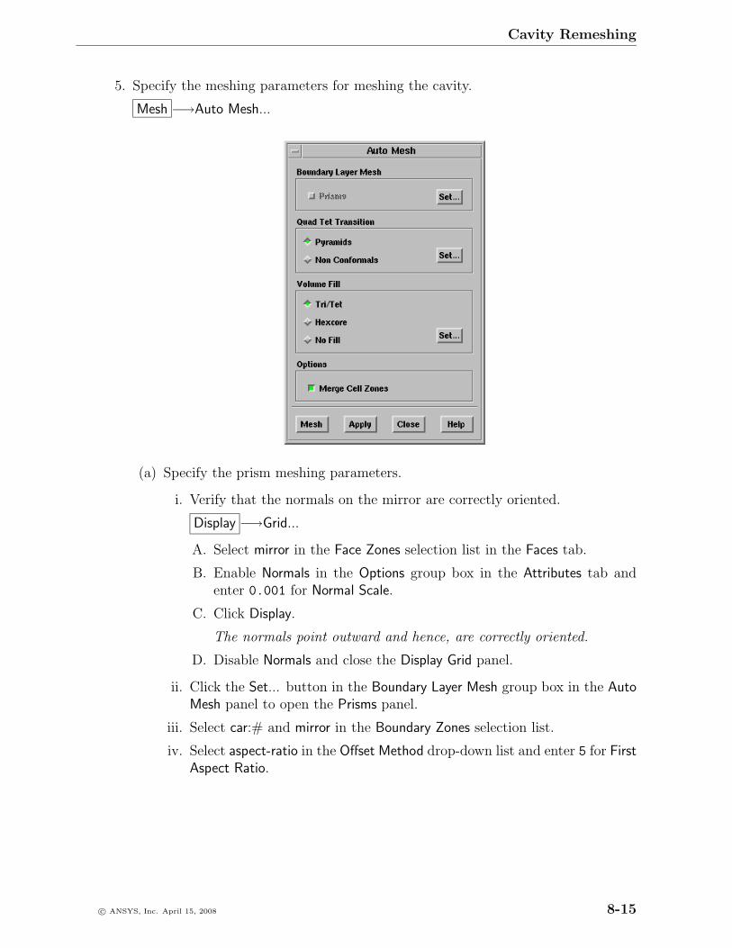
Cavity Remeshing
5. Specify the meshing parameters for meshing the cavity.
Mesh −→Auto Mesh...
(a) Specify the prism meshing parameters.
i. Verify that the normals on the mirror are correctly oriented.
Display −→Grid...
A. Select mirror in the Face Zones selection list in the Faces tab.
B. Enable Normals in the Options group box in the Attributes tab andenter 0.001 for Normal Scale.
C. Click Display.
The normals point outward and hence, are correctly oriented.
D. Disable Normals and close the Display Grid panel.
ii. Click the Set... button in the Boundary Layer Mesh group box in the AutoMesh panel to open the Prisms panel.
iii. Select car:# and mirror in the Boundary Zones selection list.
iv. Select aspect-ratio in the Offset Method drop-down list and enter 5 for FirstAspect Ratio.
c© ANSYS, Inc. April 15, 2008 8-15
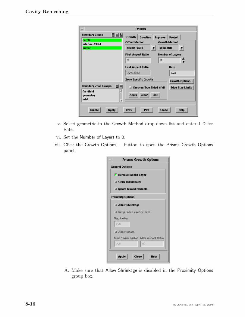
Cavity Remeshing
v. Select geometric in the Growth Method drop-down list and enter 1.2 forRate.
vi. Set the Number of Layers to 3.
vii. Click the Growth Options... button to open the Prisms Growth Optionspanel.
A. Make sure that Allow Shrinkage is disabled in the Proximity Optionsgroup box.
8-16 c© ANSYS, Inc. April 15, 2008
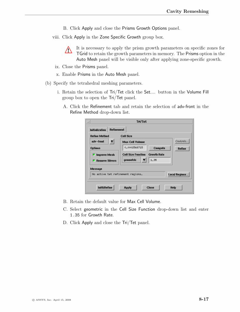
Cavity Remeshing
B. Click Apply and close the Prisms Growth Options panel.
viii. Click Apply in the Zone Specific Growth group box.
! It is necessary to apply the prism growth parameters on specific zones forTGrid to retain the growth parameters in memory. The Prisms option in theAuto Mesh panel will be visible only after applying zone-specific growth.
ix. Close the Prisms panel.
x. Enable Prisms in the Auto Mesh panel.
(b) Specify the tetrahedral meshing parameters.
i. Retain the selection of Tri/Tet click the Set.... button in the Volume Fillgroup box to open the Tri/Tet panel.
A. Click the Refinement tab and retain the selection of adv-front in theRefine Method drop-down list.
B. Retain the default value for Max Cell Volume.
C. Select geometric in the Cell Size Function drop-down list and enter1.35 for Growth Rate.
D. Click Apply and close the Tri/Tet panel.
c© ANSYS, Inc. April 15, 2008 8-17
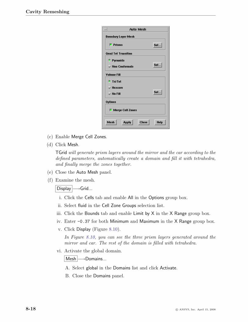
Cavity Remeshing
(c) Enable Merge Cell Zones.
(d) Click Mesh.
TGrid will generate prism layers around the mirror and the car according to thedefined parameters, automatically create a domain and fill it with tetrahedra,and finally merge the zones together.
(e) Close the Auto Mesh panel.
(f) Examine the mesh.
Display −→Grid...
i. Click the Cells tab and enable All in the Options group box.
ii. Select fluid in the Cell Zone Groups selection list.
iii. Click the Bounds tab and enable Limit by X in the X Range group box.
iv. Enter -0.37 for both Minimum and Maximum in the X Range group box.
v. Click Display (Figure 8.10).
In Figure 8.10, you can see the three prism layers generated around themirror and car. The rest of the domain is filled with tetrahedra.
vi. Activate the global domain.
Mesh −→Domains...
A. Select global in the Domains list and click Activate.
B. Close the Domains panel.
8-18 c© ANSYS, Inc. April 15, 2008
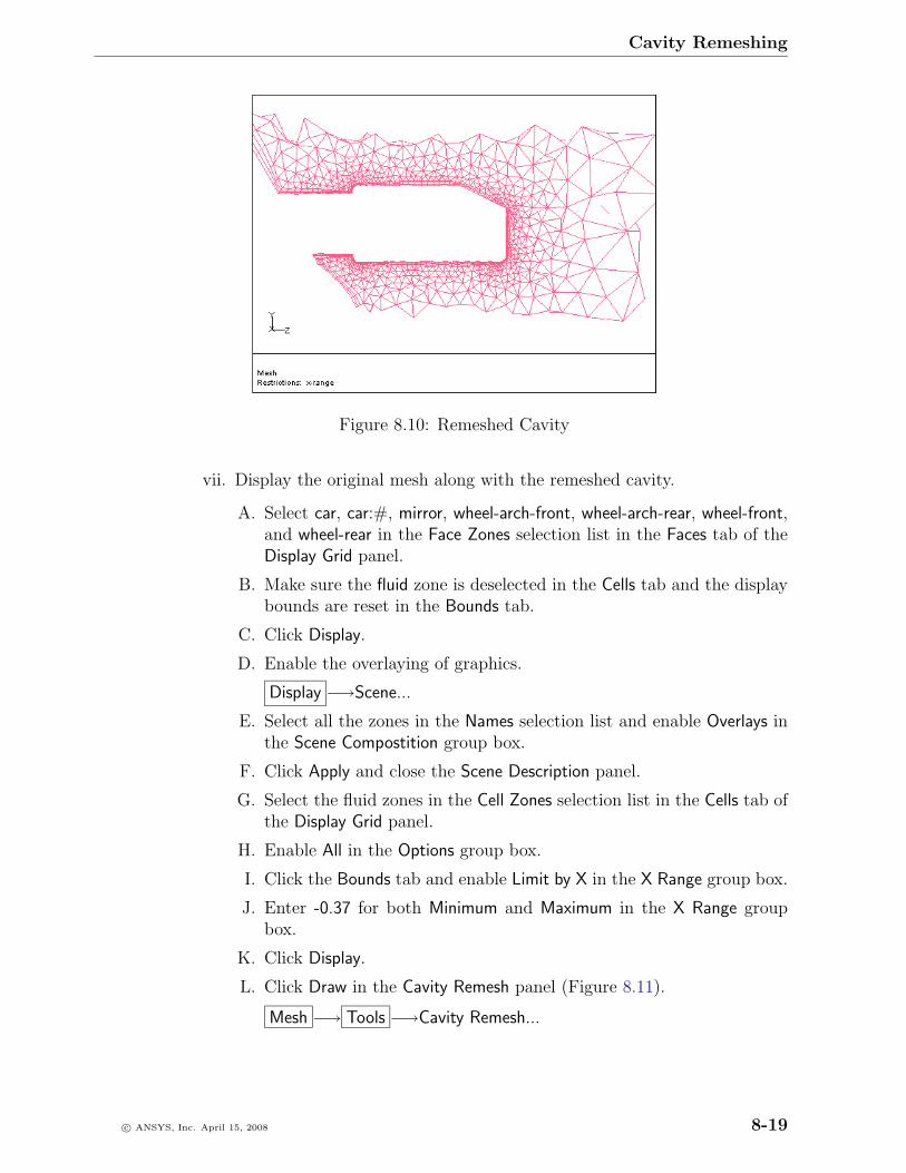
Cavity Remeshing
Figure 8.10: Remeshed Cavity
vii. Display the original mesh along with the remeshed cavity.
A. Select car, car:#, mirror, wheel-arch-front, wheel-arch-rear, wheel-front,and wheel-rear in the Face Zones selection list in the Faces tab of theDisplay Grid panel.
B. Make sure the fluid zone is deselected in the Cells tab and the displaybounds are reset in the Bounds tab.
C. Click Display.
D. Enable the overlaying of graphics.
Display −→Scene...
E. Select all the zones in the Names selection list and enable Overlays inthe Scene Compostition group box.
F. Click Apply and close the Scene Description panel.
G. Select the fluid zones in the Cell Zones selection list in the Cells tab ofthe Display Grid panel.
H. Enable All in the Options group box.
I. Click the Bounds tab and enable Limit by X in the X Range group box.
J. Enter -0.37 for both Minimum and Maximum in the X Range groupbox.
K. Click Display.
L. Click Draw in the Cavity Remesh panel (Figure 8.11).
Mesh −→ Tools −→Cavity Remesh...
c© ANSYS, Inc. April 15, 2008 8-19

Cavity Remeshing
Figure 8.11: Cavity Remeshed With Hybrid Mesh
In Figure 8.10, you can see that the mesh outside the cavity has notbeen modified. The mesh inside the cavity is connected in a conformalmanner with the original mesh.
6. Merge the cavity domain with the original mesh.
> /mesh/cavity/merge-cavity
Insert domain name/id [tet] cavity-2 <Enter>
Into domain name/id [cavity-2] global <Enter>Merging cell zone fluid-# (id #) with fluid-#Merging face zone interior-#:# (id #) with interior-#Merging face zone car:# (id #) with car
where, # denotes the respective zone IDs.
7. Delete the old mirror.
Boundary −→Manage...
(a) Select mirror-old in the Face Zones selection list.
(b) Select Delete in the Options list and retain the Delete Nodes option.
(c) Click Apply.
A Question dialog box will open asking you to confirm if you want to delete theselected zone(s).
(d) Click Yes to close the Question dialog box.
(e) Close the Manage Face Zones panel.
8-20 c© ANSYS, Inc. April 15, 2008
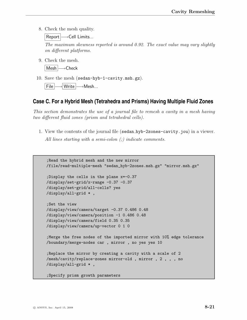
Cavity Remeshing
8. Check the mesh quality.
Report −→Cell Limits...
The maximum skewness reported is around 0.92. The exact value may vary slightlyon different platforms.
9. Check the mesh.
Mesh −→Check
10. Save the mesh (sedan-hyb-1-cavity.msh.gz).
File −→ Write −→Mesh...
Case C. For a Hybrid Mesh (Tetrahedra and Prisms) Having Multiple Fluid Zones
This section demonstrates the use of a journal file to remesh a cavity in a mesh havingtwo different fluid zones (prism and tetrahedral cells).
1. View the contents of the journal file (sedan hyb-2zones-cavity.jou) in a viewer.
All lines starting with a semi-colon (;) indicate comments.
;Read the hybrid mesh and the new mirror/file/read-multiple-mesh "sedan_hyb-2zones.msh.gz" "mirror.msh.gz"
;Display the cells in the plane x=-0.37/display/set-grid/x-range -0.37 -0.37/display/set-grid/all-cells? yes/display/all-grid * ,
;Set the view/display/view/camera/target -0.37 0.486 0.48/display/view/camera/position -1 0.486 0.48/display/view/camera/field 0.35 0.35/display/view/camera/up-vector 0 1 0
;Merge the free nodes of the imported mirror with 10% edge tolerance/boundary/merge-nodes car , mirror , no yes yes 10
;Replace the mirror by creating a cavity with a scale of 2/mesh/cavity/replace-zones mirror-old , mirror , 2 , , , no/display/all-grid * ,
;Specify prism growth parameters
c© ANSYS, Inc. April 15, 2008 8-21
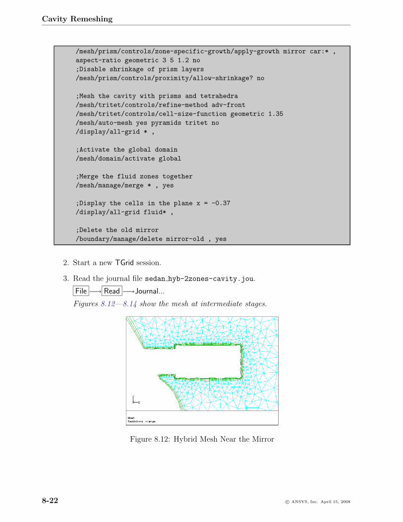
Cavity Remeshing
/mesh/prism/controls/zone-specific-growth/apply-growth mirror car:* ,aspect-ratio geometric 3 5 1.2 no;Disable shrinkage of prism layers/mesh/prism/controls/proximity/allow-shrinkage? no
;Mesh the cavity with prisms and tetrahedra/mesh/tritet/controls/refine-method adv-front/mesh/tritet/controls/cell-size-function geometric 1.35/mesh/auto-mesh yes pyramids tritet no/display/all-grid * ,
;Activate the global domain/mesh/domain/activate global
;Merge the fluid zones together/mesh/manage/merge * , yes
;Display the cells in the plane x = -0.37/display/all-grid fluid* ,
;Delete the old mirror/boundary/manage/delete mirror-old , yes
2. Start a new TGrid session.
3. Read the journal file sedan hyb-2zones-cavity.jou.
File −→ Read −→Journal...
Figures 8.12—8.14 show the mesh at intermediate stages.
Figure 8.12: Hybrid Mesh Near the Mirror
8-22 c© ANSYS, Inc. April 15, 2008
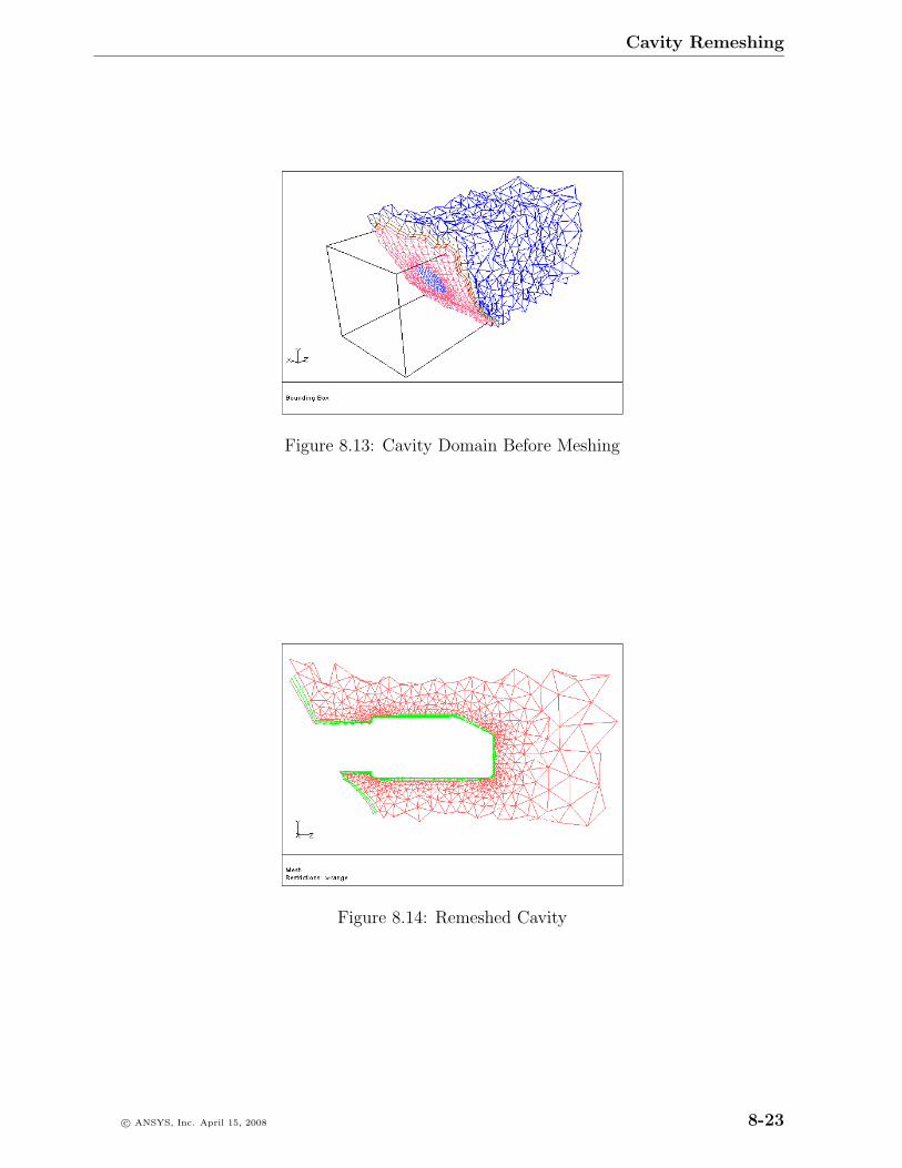
Cavity Remeshing
Figure 8.13: Cavity Domain Before Meshing
Figure 8.14: Remeshed Cavity
c© ANSYS, Inc. April 15, 2008 8-23
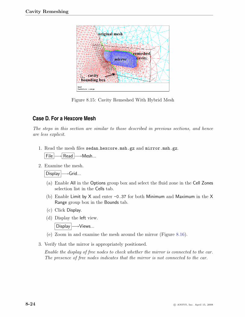
Cavity Remeshing
Figure 8.15: Cavity Remeshed With Hybrid Mesh
Case D. For a Hexcore Mesh
The steps in this section are similar to those described in previous sections, and henceare less explicit.
1. Read the mesh files sedan hexcore.msh.gz and mirror.msh.gz.
File −→ Read −→Mesh...
2. Examine the mesh.
Display −→Grid...
(a) Enable All in the Options group box and select the fluid zone in the Cell Zonesselection list in the Cells tab.
(b) Enable Limit by X and enter -0.37 for both Minimum and Maximum in the XRange group box in the Bounds tab.
(c) Click Display.
(d) Display the left view.
Display −→Views...
(e) Zoom in and examine the mesh around the mirror (Figure 8.16).
3. Verify that the mirror is appropriately positioned.
Enable the display of free nodes to check whether the mirror is connected to the car.The presence of free nodes indicates that the mirror is not connected to the car.
8-24 c© ANSYS, Inc. April 15, 2008
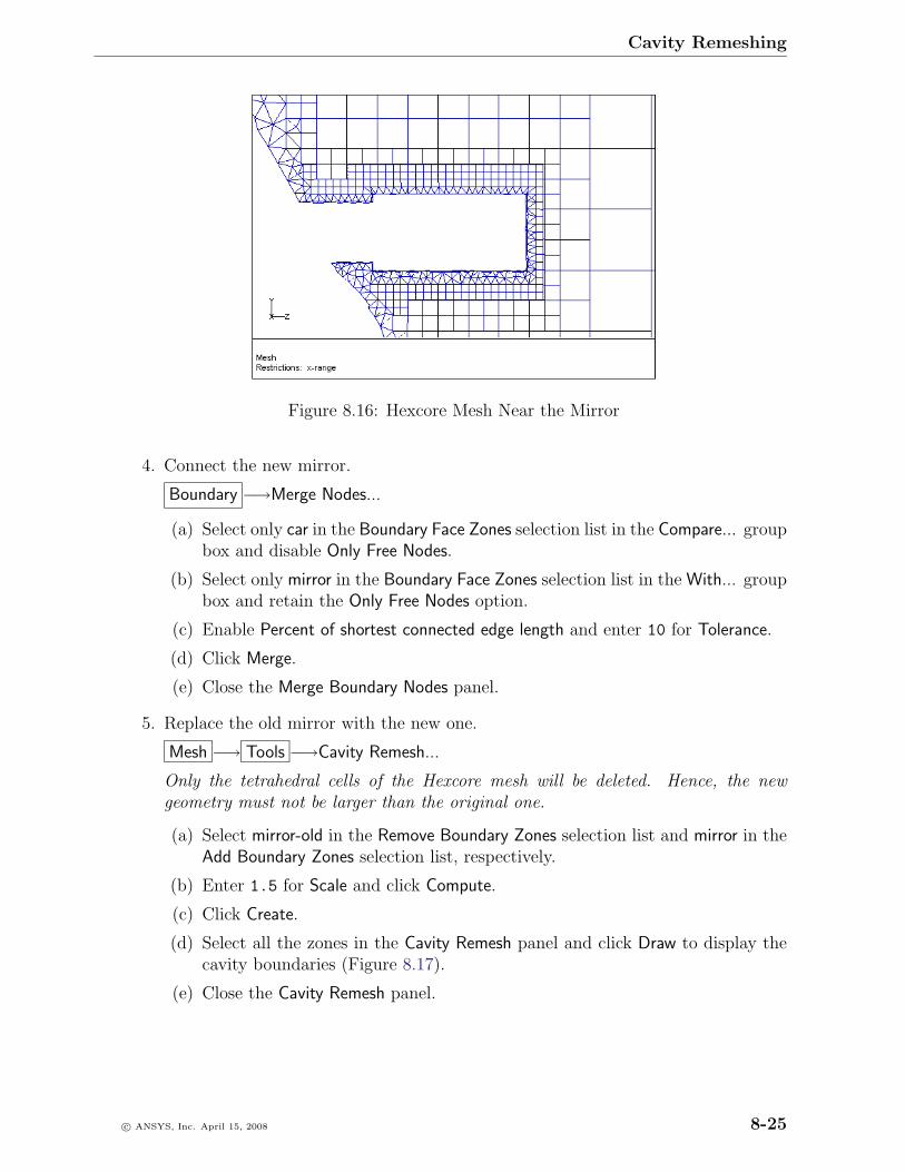
Cavity Remeshing
Figure 8.16: Hexcore Mesh Near the Mirror
4. Connect the new mirror.
Boundary −→Merge Nodes...
(a) Select only car in the Boundary Face Zones selection list in the Compare... groupbox and disable Only Free Nodes.
(b) Select only mirror in the Boundary Face Zones selection list in the With... groupbox and retain the Only Free Nodes option.
(c) Enable Percent of shortest connected edge length and enter 10 for Tolerance.
(d) Click Merge.
(e) Close the Merge Boundary Nodes panel.
5. Replace the old mirror with the new one.
Mesh −→ Tools −→Cavity Remesh...
Only the tetrahedral cells of the Hexcore mesh will be deleted. Hence, the newgeometry must not be larger than the original one.
(a) Select mirror-old in the Remove Boundary Zones selection list and mirror in theAdd Boundary Zones selection list, respectively.
(b) Enter 1.5 for Scale and click Compute.
(c) Click Create.
(d) Select all the zones in the Cavity Remesh panel and click Draw to display thecavity boundaries (Figure 8.17).
(e) Close the Cavity Remesh panel.
c© ANSYS, Inc. April 15, 2008 8-25
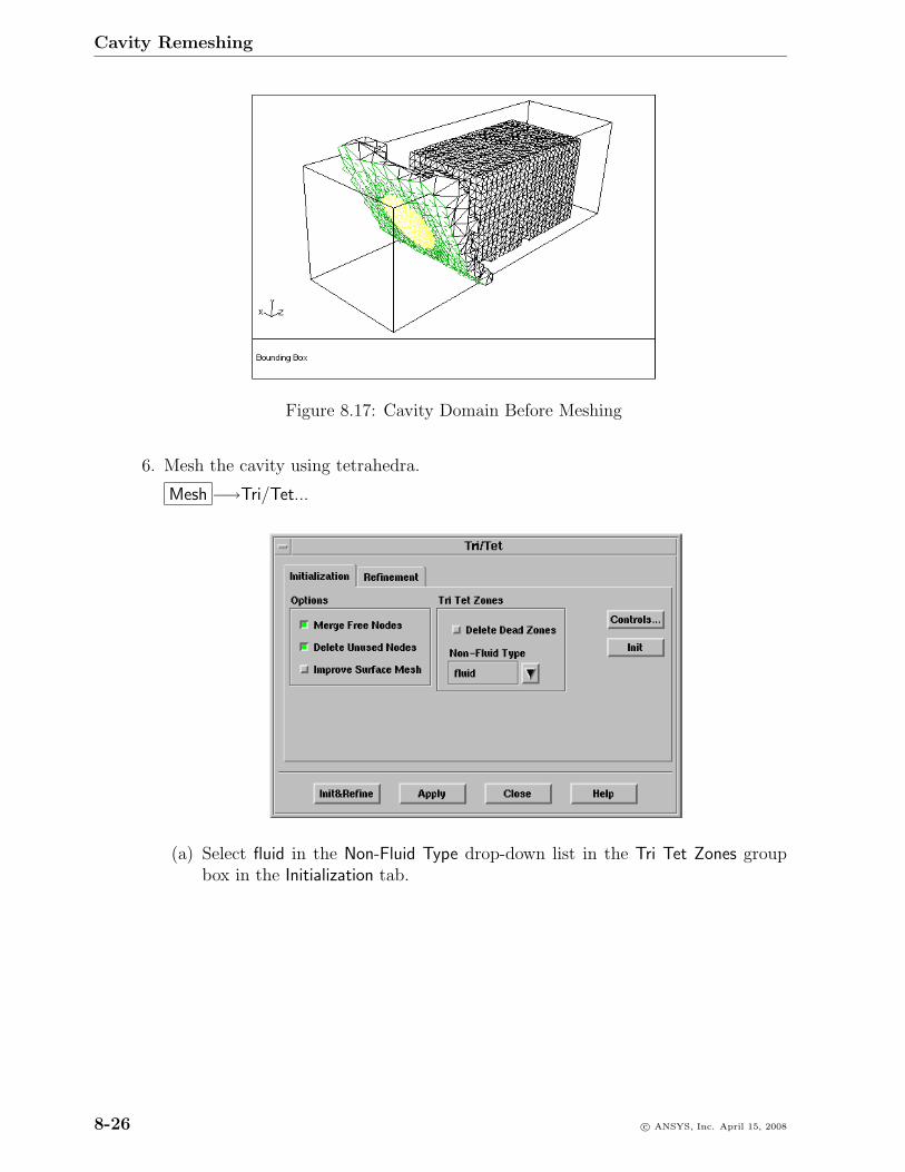
Cavity Remeshing
Figure 8.17: Cavity Domain Before Meshing
6. Mesh the cavity using tetrahedra.
Mesh −→Tri/Tet...
(a) Select fluid in the Non-Fluid Type drop-down list in the Tri Tet Zones groupbox in the Initialization tab.
8-26 c© ANSYS, Inc. April 15, 2008
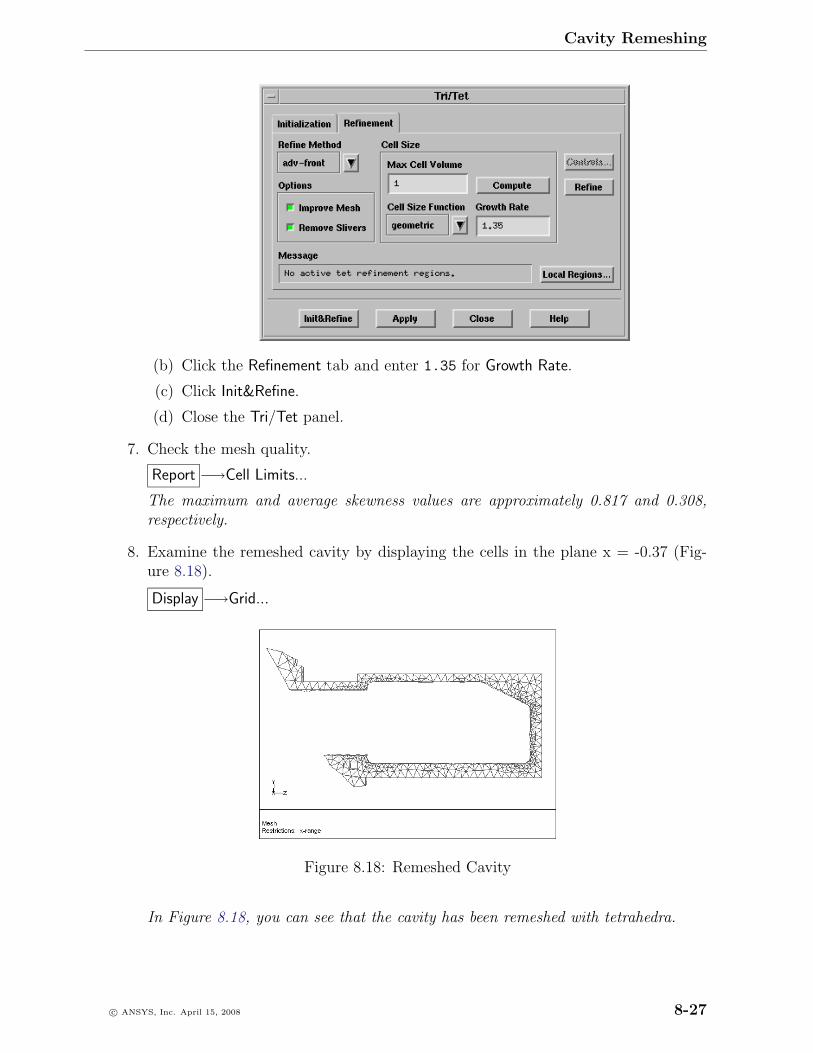
Cavity Remeshing
(b) Click the Refinement tab and enter 1.35 for Growth Rate.
(c) Click Init&Refine.
(d) Close the Tri/Tet panel.
7. Check the mesh quality.
Report −→Cell Limits...
The maximum and average skewness values are approximately 0.817 and 0.308,respectively.
8. Examine the remeshed cavity by displaying the cells in the plane x = -0.37 (Fig-ure 8.18).
Display −→Grid...
Figure 8.18: Remeshed Cavity
In Figure 8.18, you can see that the cavity has been remeshed with tetrahedra.
c© ANSYS, Inc. April 15, 2008 8-27
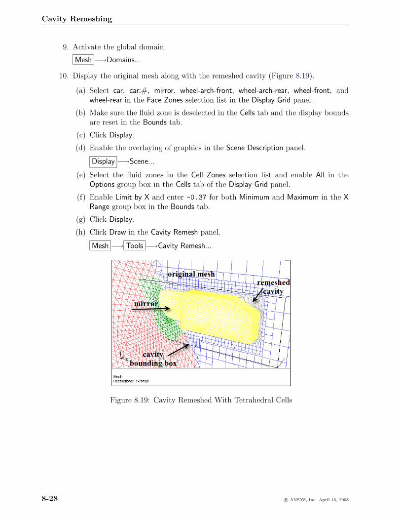
Cavity Remeshing
9. Activate the global domain.
Mesh −→Domains...
10. Display the original mesh along with the remeshed cavity (Figure 8.19).
(a) Select car, car:#, mirror, wheel-arch-front, wheel-arch-rear, wheel-front, andwheel-rear in the Face Zones selection list in the Display Grid panel.
(b) Make sure the fluid zone is deselected in the Cells tab and the display boundsare reset in the Bounds tab.
(c) Click Display.
(d) Enable the overlaying of graphics in the Scene Description panel.
Display −→Scene...
(e) Select the fluid zones in the Cell Zones selection list and enable All in theOptions group box in the Cells tab of the Display Grid panel.
(f) Enable Limit by X and enter -0.37 for both Minimum and Maximum in the XRange group box in the Bounds tab.
(g) Click Display.
(h) Click Draw in the Cavity Remesh panel.
Mesh −→ Tools −→Cavity Remesh...
Figure 8.19: Cavity Remeshed With Tetrahedral Cells
8-28 c© ANSYS, Inc. April 15, 2008
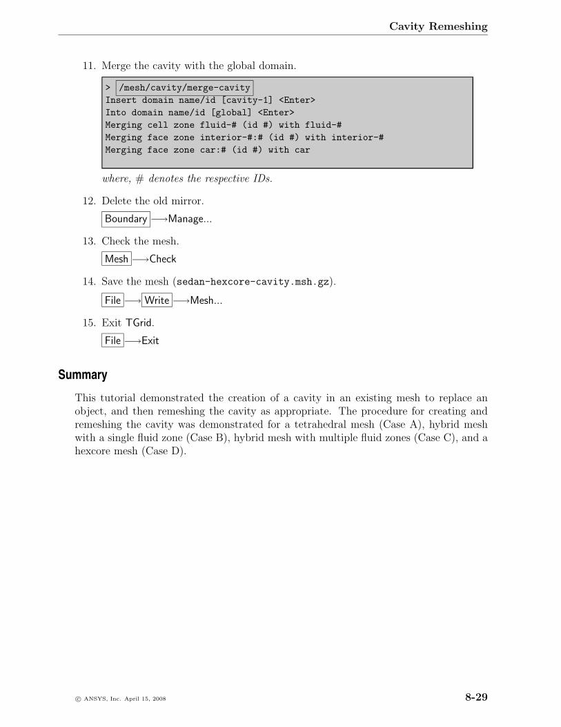
Cavity Remeshing
11. Merge the cavity with the global domain.
> /mesh/cavity/merge-cavityInsert domain name/id [cavity-1] <Enter>Into domain name/id [global] <Enter>Merging cell zone fluid-# (id #) with fluid-#Merging face zone interior-#:# (id #) with interior-#Merging face zone car:# (id #) with car
where, # denotes the respective IDs.
12. Delete the old mirror.
Boundary −→Manage...
13. Check the mesh.
Mesh −→Check
14. Save the mesh (sedan-hexcore-cavity.msh.gz).
File −→ Write −→Mesh...
15. Exit TGrid.
File −→Exit
Summary
This tutorial demonstrated the creation of a cavity in an existing mesh to replace anobject, and then remeshing the cavity as appropriate. The procedure for creating andremeshing the cavity was demonstrated for a tetrahedral mesh (Case A), hybrid meshwith a single fluid zone (Case B), hybrid mesh with multiple fluid zones (Case C), and ahexcore mesh (Case D).
c© ANSYS, Inc. April 15, 2008 8-29

Cavity Remeshing
8-30 c© ANSYS, Inc. April 15, 2008