Fluid Dynamicsby Finite Element AnalysisIrrotational and Viscous Flow in 2D and 3D

Using FlexPDE Version 5

Gunnar Backstrom

This electronic book is available in the form of Adobe® Acrobat®

5.0 PDF files. It may also be read using later versions of the program.The reader may not transfer the PDF file to other persons, in any formor by any means. You may print the text for your private purposes butnot transfer copies to others.

How to Start Reading

Double-click on the PDF icon to start the Adobe® Acrobat® Reader.View the list of contents by pushing the F5 keyboard button.

Toggle by F5 to view the text only.

Copyright © 2005by GB Publishing® and Gunnar Backstrom

Malmo, Sweden

All rights reserved.

Preface

This book is a sequel to the e-book Deformation and Vibration byFinite Element Analysis. The present volume hence starts withChapter 18. Using the same software (FlexPDE version 5) it expandsthe applications to irrotational and viscous flow of incompressiblefluids.

The preceding part started with an introductory chapter ongraphical facilities, which may be studied without applying boundaryconditions and without solving any PDE. There seems to be no reasonto repeat this material here, and hence it is omitted.

As before, there is no index since the Acrobat program lets yousearch for words and even word combinations. After selecting Edit,Find (or pushing the keys Ctrl+f) if suffices to enter the item ofinterest. The table of contents is also available and may be brought upto the left of the text by clicking on Bookmarks (or by pushing F5). Asimple click on a subtitle opens that section immediately.

Since this is the last of the four Fields volumes, I should again liketo thank my late friend Dr. Russell Ross, University of East Anglia,for reading and commenting the work. The admirable programmerbehind FlexPDE, Mr. Bob Nelson, kindly continued to support thisfinal round of applications.

Gunnar Backstrom

The finite-element software package used for this book (FlexPDE) ismarketed by

PDE Solutions IncPO Box 4217, Antioch, CA 94531-4217, USAPhone: +1 925 776 2407 Fax: +1 925 776 2406Email: sales@pdesolutions.comhttp://www.pdesolutions.com

Contents

18 Irrotational Flow of Liquids in (x,y) Space 226 Flow through a Constricted Channel 227 Cylindrical Obstacle across a Straight Channel 231 Obstacle Close to a Wall 234 Drag and Lift on an Inclined Plate 23519 Circulation around an Obstacle 240 Circulation Integral 243 Combined Velocity Fields 244 Forces on an Inclined Plate 24820 Viscous Flow in Channels 252 Boundary Conditions 255 Steady Flow at Small Speeds (Re<<1) 256 Flow Due to a Moving Wall at Re<<1 257 Pressure-Driven Flow through a Channel 259 Viscous Flow through a Constricted Channel 262 Comparison with Irrotational Flow 266 Tangential Input Velocity 267 Channel with a Lateral Cavity 269 Uniform Velocity of Injection 271 Dynamic Similarity 27221 Viscous Flow past an Obstacle 277 Viscous Flow past a Circular Cylinder 277 Viscous Force on a Solid Surface 280 Forces on a Circular Cylinder 282 Force Equilibrium 283 Viscous Dissipation 285 Drag and Lift on an Inclined Plate 287

22 Irrotational Flow in (ρ,z) Space 290 Constricted Tube 291 Constricted Tube with a Spherical Obstacle 294

23 Viscous Flow in (ρ,z) Space 297 Boundary Conditions 298 Steady Flow at Small Speeds 299 Tube with Uniform Driving Pressure 300 Tube with Uniform Input Velocity 302 Viscous Flow by Gravity through a Funnel 305 Forces on the Funnel 307 Dissipation in the Funnel 308 Viscous Flow past a Sphere 310 Comparison with an Analytic Solution 31224 Seeping through Porous Materials 316 Percolation in (x,y) Space 316 Percolation in (x,y) by Navier-Stokes PDE 318 Percolation in (ρ,z) Space 322 Percolation in (ρ,z) by Navier-Stokes 32425 Viscous Flow at Re>>1 in (x,y) 328 Viscous Flow in a Channel 329 Viscous Flow past a Circular Cylinder 332 Viscous Boundary Layer 335 Viscous Flow past a Rotating Cylinder 337 Viscous Flow past an Inclined Plate 340 Viscous Flow past an Airfoil 34326 Viscous Flow at Re>>1 in (ρ,z) 346 Parabolic Velocity Injection into a Tube 348 Jet into a Liquid 350 Viscous Flow Past a Sphere 35227 Transient Viscous Flow at Re<<1 355 Transient Flow due to a Moving Wall in (x,y) 356 Transient Flow due to a Localized Force 357 Heat Transport by Conduction and Convection 361

Natural Convection in (x,y) 363 Natural Convection in (ρ,z) 36628 Viscous Flow in Three Dimensions 369 Extension of the Formalism to 3D 369 Flow through a Rectangular Duct 370 Flow through a Box with Two Orifices 374 Viscous Flow around a Cubical Obstacle 377 Viscous Flow by Gravity through a Funnel 380 Rotating Flow through a Funnel 383 Seeping through a Concrete Plate with a Pillar 38529 Simplified PDEs for Viscous Flow 389 Steady Flow in a Constricted Channel at Re<<1 390 Flow past a Circular Cylinder at Re<<1 392 Flow through a Box with Two Orifices (3D) 394 Steady Viscous Flow at Re>>1 396 Flow past a Circular Cylinder at Re>>1 397 Flow in (ρ,z) past a Sphere at Re>>1 399References 402

Vocabulary 403

226

18 Irrotational Flow of Liquids in (x,y)

This is the second volume on mechanical fields, and the introductorychapters on graphics, Laplace, and Poisson equations will not berepeated here. Instead, we occasionally refer to the preceding bookfor elementary details.

Since the density of a liquid normally changes little within therange of pressures occurring in practical applications, we assume thedensity to be constant. In this chapter we also make more daringassumptions, i.e. that the liquid slips freely over solid surfaces andthat viscous forces are vanishingly small compared to inertial forces.These assumptions are known to be useful, however, in manysituations.

The conservation of mass may be expressed as8p52

∇⋅ = −( )ρ ∂ρ∂0

0vt

where ρ0 is the mass density and v the velocity vector. Assumingconstant density, this leads us to the conservation of volume∇⋅ =v 0

or in explicit form

∂∂

∂∂

vx

vy

x y+ = 0

This PDE is not of 2nd order, which is a prerequisite for solving itby FlexPDE. Fortunately, we may arrange this by expressing thevelocity components as derivatives of a common function φ . Hence,let us choose the definitions

vxx =

∂φ∂

, vyy =

∂φ∂

In this manner we arrive at

227

∂ φ∂

∂ φ∂

2

2

2

2 0x y+ =

which is the well known Laplace equation (see Chapter 5 inDeformation and Vibration).

So far, we have only used the principle of conservation of mass,but it is important to note that any solution to the above PDE will alsobe irrotational (∇× =v 0), because

∇× = − = − =va fz y xvx

vy x y y x

∂∂

∂∂

∂ φ∂ ∂

∂ φ∂ ∂

2 20

Energy conservation next leads us to the Bernoulli equation ofmotion, which states8p116

12 0

20ρ ρv p g y+ + = constant

where v v vx y= +2 2 is the magnitude of the velocity (speed), p thepressure, and g the acceleration due to gravity (assuming the y-axis tobe vertical).

Flow through a Constricted Channel

Our first application of the above equations will be to the flowthrough a horizontal channel, limited by plane surfaces perpendicularto our domain.

The following descriptor defines the problem and introduces thePDE for the velocity potential φ . After solving for phi we simplydifferentiate to obtain the components of velocity. Having obtainedthese components we then form the magnitude of the velocity (v).Assuming horizontal flow, where the gravity terms cancel, theBernoulli equation gives us12

120

20 0

20ρ ρv p v p+ = +

and we finally obtain the expression for the pressure p included in thedefinitions segment.

228

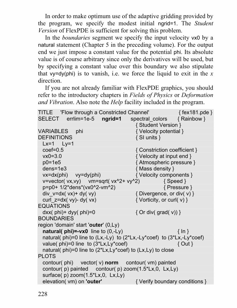
In order to make optimum use of the adaptive gridding provided bythe program, we specify the modest initial ngrid=1. The StudentVersion of FlexPDE is sufficient for solving this problem.

In the boundaries segment we specify the input velocity vx0 by anatural statement (Chapter 5 in the preceding volume). For the outputend we just impose a constant value for the potential phi. Its absolutevalue is of course arbitrary since only the derivatives will be used, butby specifying a constant value over this boundary we also stipulatethat vy=dy(phi) is to vanish, i.e. we force the liquid to exit in the xdirection.

If you are not already familiar with FlexPDE graphics, you shouldrefer to the introductory chapters in Fields of Physics or Deformationand Vibration. Also note the Help facility included in the program.TITLE 'Flow through a Constricted Channel' { fex181.pde }SELECT errlim=1e-5 ngrid=1 spectral_colors { Rainbow } { Student Version }VARIABLES phi { Velocity potential }DEFINITIONS { SI units } Lx=1 Ly=1 coef=0.5 { Constriction coefficient } vx0=3.0 { Velocity at input end } p0=1e5 { Atmospheric pressure } dens=1e3 { Mass density } vx=dx(phi) vy=dy(phi) { Velocity components } v=vector( vx,vy) vm=sqrt( vx^2+ vy^2) { Speed } p=p0+ 1/2*dens*(vx0^2-vm^2) { Pressure } div_v=dx( vx)+ dy( vy) { Divergence, or div( v) } curl_z=dx( vy)- dy( vx) { Vorticity, or curl( v) }EQUATIONS dxx( phi)+ dyy( phi)=0 { Or div( grad( v)) }BOUNDARIESregion 'domain' start 'outer' (0,Ly) natural( phi)=-vx0 line to (0,-Ly) { In } natural( phi)=0 line to (Lx,-Ly) to (2*Lx,-Ly*coef) to (3*Lx,-Ly*coef) value( phi)=0 line to (3*Lx,Ly*coef) { Out } natural( phi)=0 line to (2*Lx,Ly*coef) to (Lx,Ly) to closePLOTS contour( phi) vector( v) norm contour( vm) painted contour( p) painted contour( p) zoom(1.5*Lx,0, Lx,Ly) surface( p) zoom(1.5*Lx,0, Lx,Ly) elevation( vm) on 'outer' { Verify boundary conditions }

229

contour( div_v) contour( curl_z)END

The modifier norm here follows the vector plot command. Thismeans that the arrows will be normalized to a standard length, but thecolor code indicates the magnitude, i.e. the speed. This plot showsthat the speed is constant across the ends and that there is an increasefrom input to output. The elevation plot on the boundary shows thisfact more clearly.

The vector plot below thus represents the velocity field. We noticethat the streamlines are parallel to the boundaries, where they comeclose, but the speed does not vanish there. We also notice that thespeed distribution at the exit appears to be roughly twice that at theentrance.

We also see from the plot of vm (not shown here) that the speedincreases by a factor of about two from input to output, i.e. in inverseproportion to the channel width. This is of course in accord with theconservation of mass and volume, a principle that was incorporatedinto the PDE by the vanishing divergence. Notice, however, that wedid not explicitly introduce this constancy in the boundary conditionsat the ends, although we could well have done so.

230

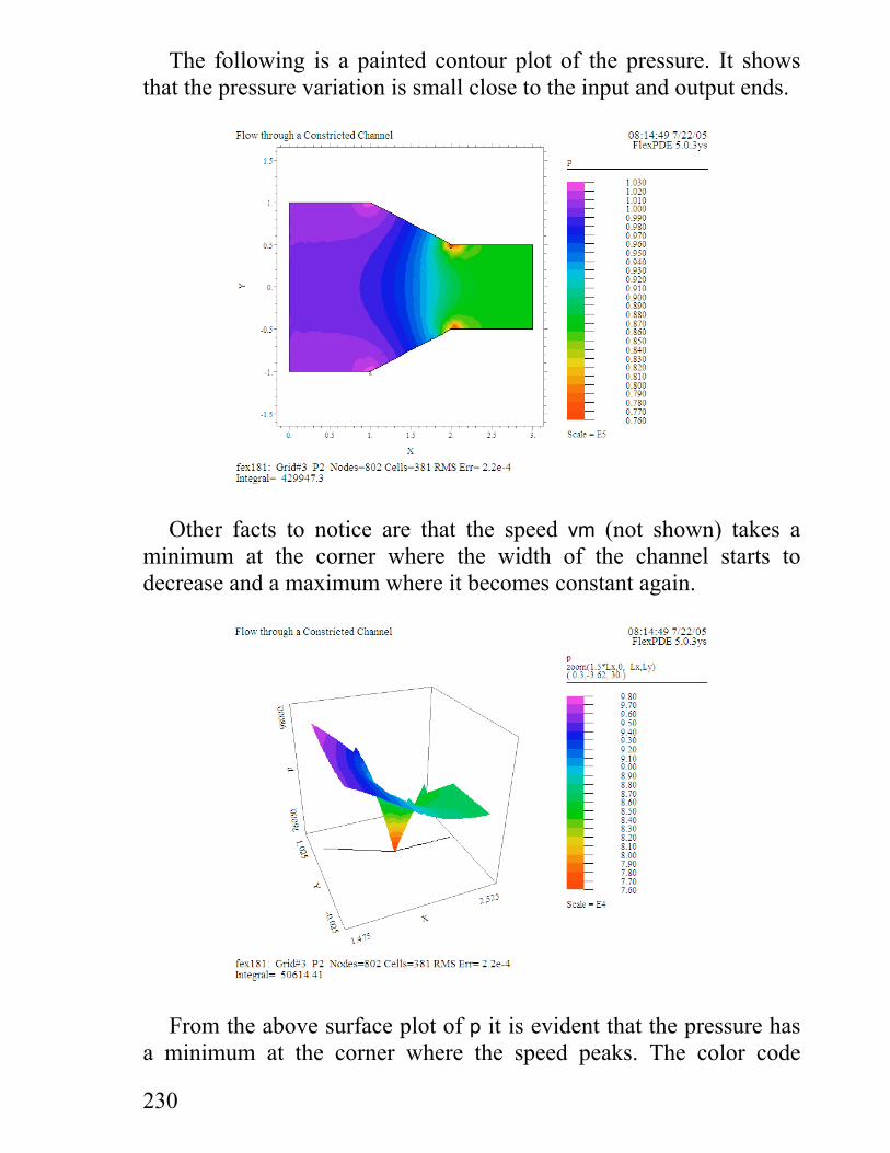
The following is a painted contour plot of the pressure. It showsthat the pressure variation is small close to the input and output ends.

Other facts to notice are that the speed vm (not shown) takes aminimum at the corner where the width of the channel starts todecrease and a maximum where it becomes constant again.

From the above surface plot of p it is evident that the pressure hasa minimum at the corner where the speed peaks. The color code

231

indicates that this minimum is about 70% of the value at the inputend, as gathered from the un-zoomed plot. From the latter plot wealso deduce that the pressure decreases from input to output, but notin proportion to the width.

The last two plots demonstrate that the divergence as well as thecurl of the velocity field vanishes.

Cylindrical Obstacle across a Straight Channel

We shall next consider flow around an obstacle, and in particular theforces exerted on it by the stream. In the descriptor, which is based onfex181, we introduce a bar of circular cross-section across thechannel.TITLE 'Obstacle across a Straight Channel' { fex182.pde }SELECT errlim=1e-4 ngrid=1 spectral_colorsVARIABLES phi { Velocity potential }DEFINITIONS Lx=1.0 Ly=1.0 a=0.2 vx0=5.0 { x-component of velocity at left end } p0=1e5 { Atmospheric pressure at left end } dens=1e3 { Mass density } vx=dx( phi) vy=dy( phi) { Velocity components } v=vector( vx,vy) vm=magnitude( v) p=p0+ 0.5*dens*( vx0^2- vm^2) { Pressure }EQUATIONS div( grad( phi))=0BOUNDARIESregion 'domain' start 'outer' (-Lx,Ly) point value( phi)= 0 natural( phi)=-vx0 line to (-Lx,-Ly) { In } natural( phi)=0 line to (Lx,-Ly) { Wall } natural( phi)=vx0 line to (Lx,Ly) { Out } natural( phi)=0 line to close { Wall } start 'obstacle' (a,0) { Cut-out } natural( phi)=0 arc( center=0,0) angle=360 closePLOTS contour( vm) painted vector( v) norm vector( v) norm zoom(-3*a/2,-a/2, 2*a,2*a) contour( p) painted elevation( p) on 'obstacle'END

232

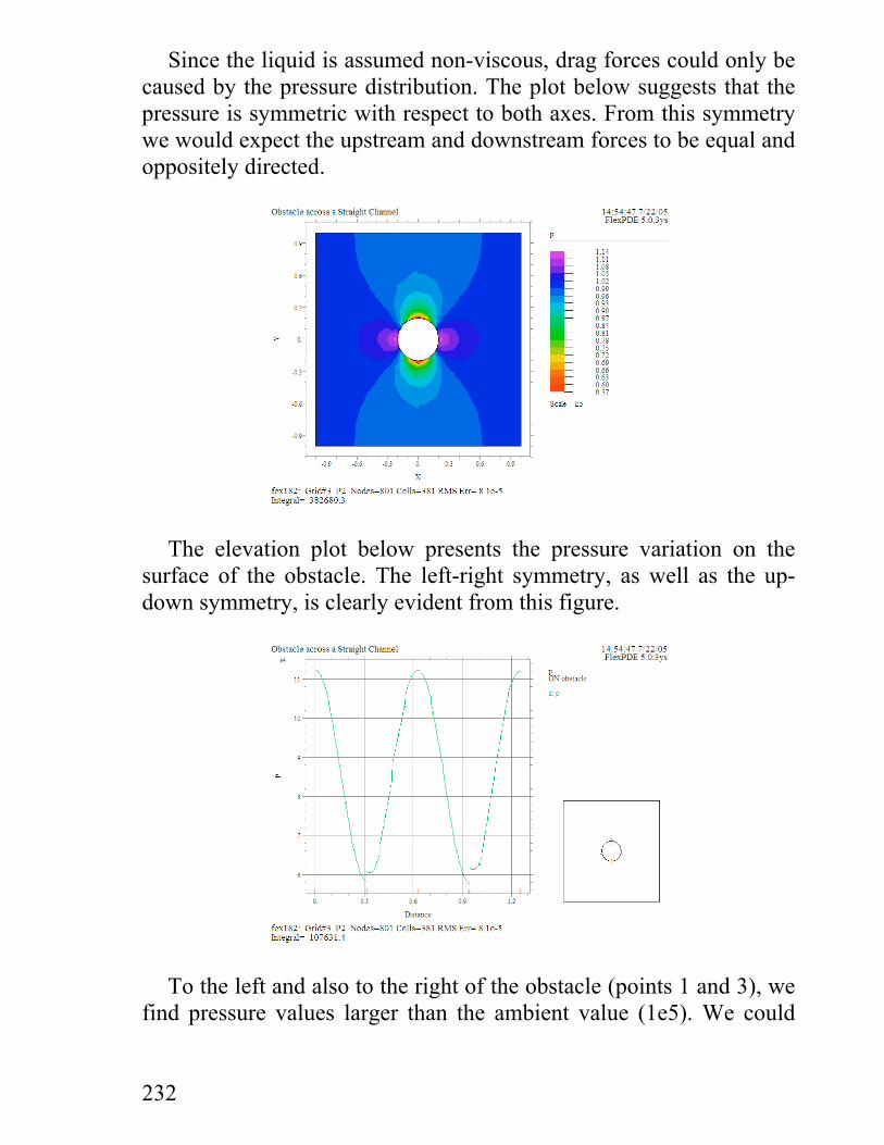
Since the liquid is assumed non-viscous, drag forces could only becaused by the pressure distribution. The plot below suggests that thepressure is symmetric with respect to both axes. From this symmetrywe would expect the upstream and downstream forces to be equal andoppositely directed.

The elevation plot below presents the pressure variation on thesurface of the obstacle. The left-right symmetry, as well as the up-down symmetry, is clearly evident from this figure.

To the left and also to the right of the obstacle (points 1 and 3), wefind pressure values larger than the ambient value (1e5). We could

233

also calculate this maximum value directly from the Bernoulliequation (p.227 2)12

12

202

0ρ ρv p v p+ = +

for a point of flow stagnation ( )v = 0 , obtaining the result p=1.125e5.The pressure on the sides parallel to the mainstream (points 2 and

4) is much lower than the ambient value. This pressure reduction is awell-known consequence of the Bernoulli equation.

The left-right symmetry of the pressure plot indicates the absenceof a force dragging the object along the stream. This may be sur-prising at first. As is apparent from the following vector plot,however, the incoming flow deviates to become parallel to the frontface, but the acceleration required is equal and opposite to thatrequired for making the stream parallel again on the opposite side.

The plot also illustrates the phenomenon of stagnation. The colorserves to indicate the magnitude. Here, the speed vanishes at y = 0 ona line perpendicular to the figure.

It is clear from the above (symmetric) plots of p that the pressureforces on the liquid sum to the value zero. Since the liquid slips onthe boundaries, the total force vanishes, and hence the force on theobstacle.

234

Even if there is no resultant force on the cylinder, we do findexcess pressure on the left and right sides and a deficit at the bottomand top sides. Hence, if the obstacle were elastic it would deform.

Obstacle Close to a Wall

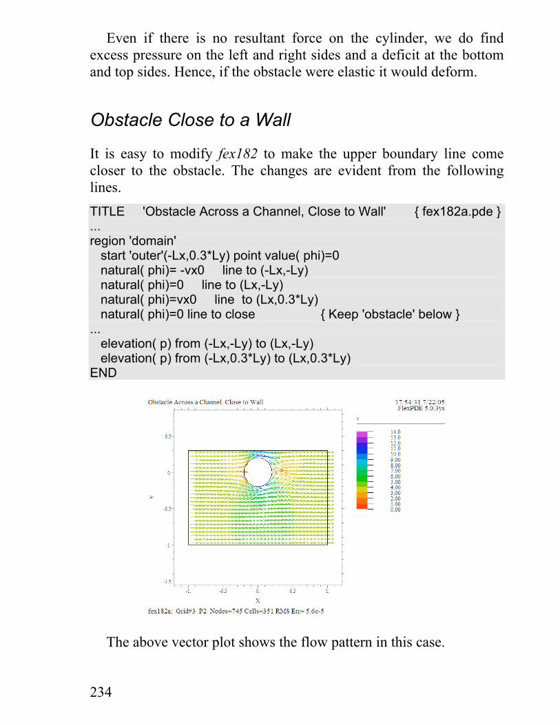
It is easy to modify fex182 to make the upper boundary line comecloser to the obstacle. The changes are evident from the followinglines.TITLE 'Obstacle Across a Channel, Close to Wall' { fex182a.pde }...region 'domain' start 'outer'(-Lx,0.3*Ly) point value( phi)=0 natural( phi)= -vx0 line to (-Lx,-Ly) natural( phi)=0 line to (Lx,-Ly) natural( phi)=vx0 line to (Lx,0.3*Ly) natural( phi)=0 line to close { Keep 'obstacle' below }... elevation( p) from (-Lx,-Ly) to (Lx,-Ly) elevation( p) from (-Lx,0.3*Ly) to (Lx,0.3*Ly)END

The above vector plot shows the flow pattern in this case.

235

As is evident from the following plot, p is still left-right symmetric,but the pressure is now lower on the top than at the bottom of thecylinder. From this it is clear that an upward force acts on theobstacle.

Evidently, the pressure pushes the obstacle toward the nearby wall.This effect is vaguely analogous to the suction felt when you standclose to a passing train.

The elevation plots present the pressure on the top and bottomsides of the domain, and from these we may read off the integrals,which are equal to the forces on the liquid, caused by the cylinder.The conclusion is that the force on the latter is 195527-188798=6729.

Drag and Lift on an Inclined Plate

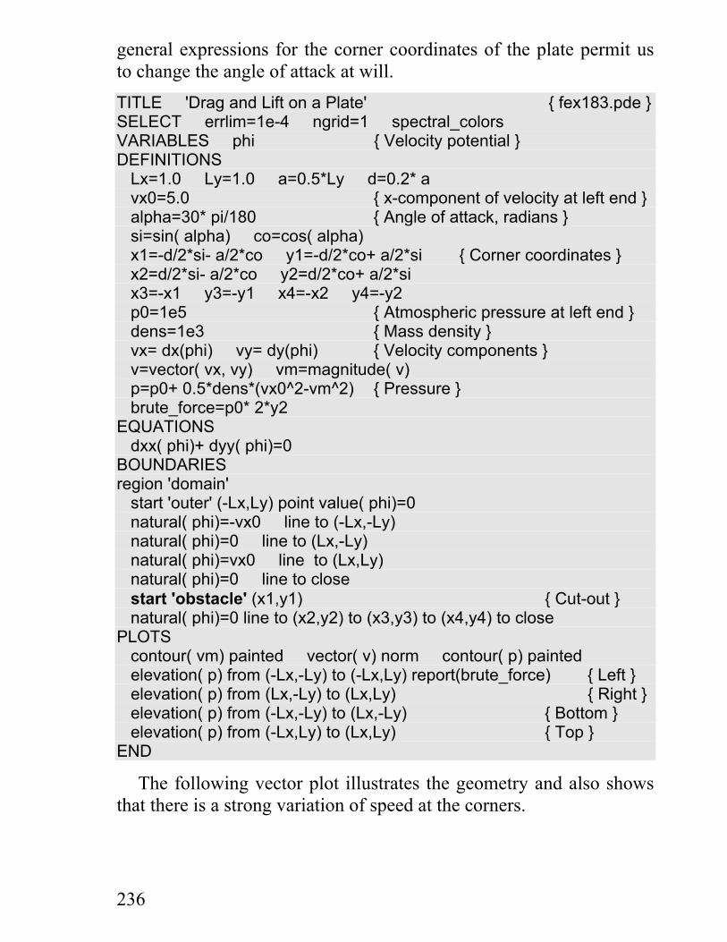
Let us now turn to a situation where we all know from experience thata lifting force may occur, both in air and in water. The geometryshould be clear from the figure below. As before, we have a stream ofliquid from left to right with constant velocity at the verticalboundaries. In the following descriptor the obstacle is a rectangularplate at an angle of attack (alpha) with respect to the main stream. The

236

general expressions for the corner coordinates of the plate permit usto change the angle of attack at will.TITLE 'Drag and Lift on a Plate' { fex183.pde }SELECT errlim=1e-4 ngrid=1 spectral_colorsVARIABLES phi { Velocity potential }DEFINITIONS Lx=1.0 Ly=1.0 a=0.5*Ly d=0.2* a vx0=5.0 { x-component of velocity at left end } alpha=30* pi/180 { Angle of attack, radians } si=sin( alpha) co=cos( alpha) x1=-d/2*si- a/2*co y1=-d/2*co+ a/2*si { Corner coordinates } x2=d/2*si- a/2*co y2=d/2*co+ a/2*si x3=-x1 y3=-y1 x4=-x2 y4=-y2 p0=1e5 { Atmospheric pressure at left end } dens=1e3 { Mass density } vx= dx(phi) vy= dy(phi) { Velocity components } v=vector( vx, vy) vm=magnitude( v) p=p0+ 0.5*dens*(vx0^2-vm^2) { Pressure } brute_force=p0* 2*y2EQUATIONS dxx( phi)+ dyy( phi)=0BOUNDARIESregion 'domain' start 'outer' (-Lx,Ly) point value( phi)=0 natural( phi)=-vx0 line to (-Lx,-Ly) natural( phi)=0 line to (Lx,-Ly) natural( phi)=vx0 line to (Lx,Ly) natural( phi)=0 line to close start 'obstacle' (x1,y1) { Cut-out } natural( phi)=0 line to (x2,y2) to (x3,y3) to (x4,y4) to closePLOTS contour( vm) painted vector( v) norm contour( p) painted elevation( p) from (-Lx,-Ly) to (-Lx,Ly) report(brute_force) { Left } elevation( p) from (Lx,-Ly) to (Lx,Ly) { Right } elevation( p) from (-Lx,-Ly) to (Lx,-Ly) { Bottom } elevation( p) from (-Lx,Ly) to (Lx,Ly) { Top }END

The following vector plot illustrates the geometry and also showsthat there is a strong variation of speed at the corners.

237

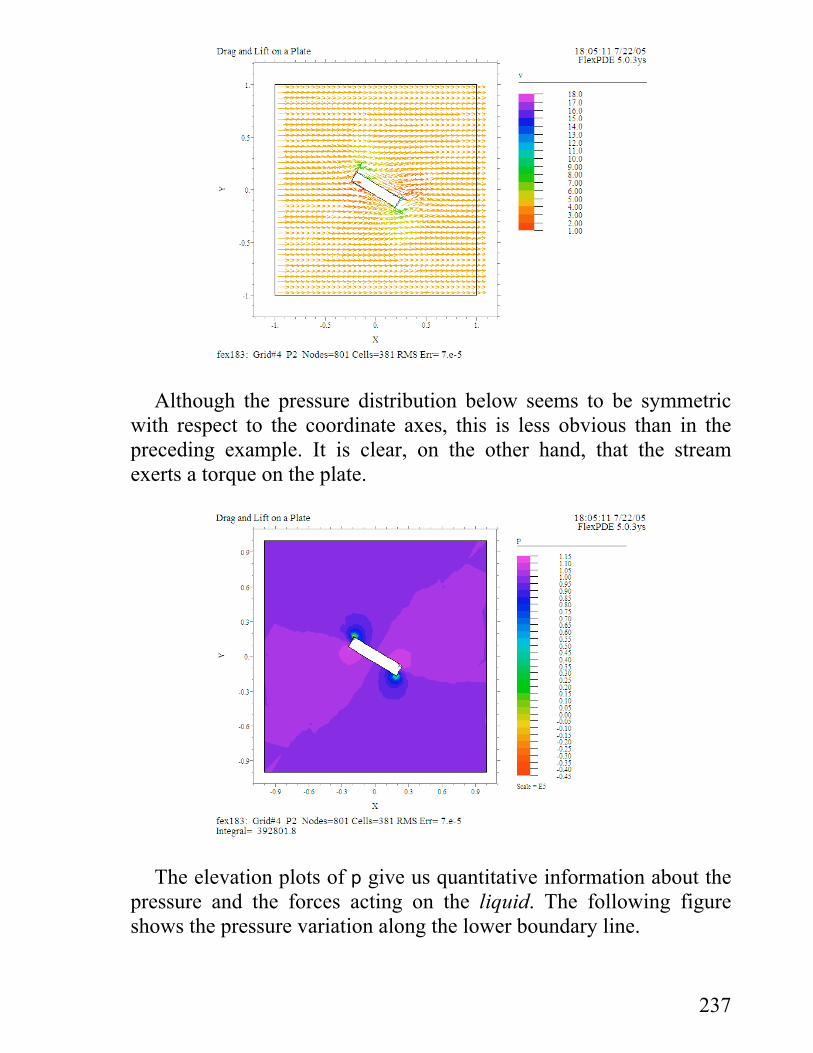
Although the pressure distribution below seems to be symmetricwith respect to the coordinate axes, this is less obvious than in thepreceding example. It is clear, on the other hand, that the streamexerts a torque on the plate.

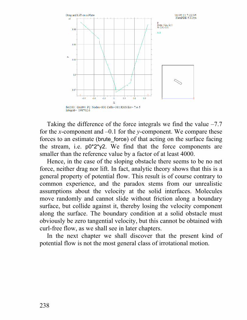
The elevation plots of p give us quantitative information about thepressure and the forces acting on the liquid. The following figureshows the pressure variation along the lower boundary line.

238

Taking the difference of the force integrals we find the value –7.7for the x-component and –0.1 for the y-component. We compare theseforces to an estimate (brute_force) of that acting on the surface facingthe stream, i.e. p0*2*y2. We find that the force components aresmaller than the reference value by a factor of at least 4000.

Hence, in the case of the sloping obstacle there seems to be no netforce, neither drag nor lift. In fact, analytic theory shows that this is ageneral property of potential flow. This result is of course contrary tocommon experience, and the paradox stems from our unrealisticassumptions about the velocity at the solid interfaces. Moleculesmove randomly and cannot slide without friction along a boundarysurface, but collide against it, thereby losing the velocity componentalong the surface. The boundary condition at a solid obstacle mustobviously be zero tangential velocity, but this cannot be obtained withcurl-free flow, as we shall see in later chapters.

In the next chapter we shall discover that the present kind ofpotential flow is not the most general class of irrotational motion.

239

Exercises

Change the boundary condition at the output end of the constrictedchannel (fex181), such that you specify the appropriate horizontalvelocity. Compare the results to those of the original example. Thenchange the output speed in the boundary condition by 10 % andobserve the consequences.

Change fex181 so that the horizontal input velocity will varyacross the channel according to the function u y Lx y0

23 1= −[ ( / ) ],still keeping φ equal to zero at the output end.

Use an input speed of 7.0 m/s in fex181 and notice the minimumvalue of pressure resulting from the solution. Suggest a physicalinterpretation of the astonishing outcome.

Change the angle of attack and the thickness of the inclined plate(fex183) according to your own taste.

Expand fex181 to fit the simplest model of a symmetrical Venturitube8p120.

240

19 Circulation around an Obstacle

In the preceding chapter on potential flow we obtained velocity fieldswith vanishing curl, known as irrotational. We shall now find thatwhenever there is an obstacle in the stream, alternative irrotationalsolutions exist. By adding such a solution to that of potential flow weobtain a more general kind of motion.

Let us start from the expression for the curl component relevant tomotion in the ( , )x y plane.

∇× = − =va fz y xvx

vy

∂∂

∂∂

ω

The quantity ω is usually called vorticity. In irrotational flow, thevorticity has to vanish everywhere in the liquid, but the velocity fieldinside the obstacle does not have to obey this condition. Of course,nothing will be moving in the solid obstacle, but the solution mayformally extend into this region.

The problem at hand is to solve the above PDE, which is of firstorder only. We thus proceed as on p.226 to transform it into astandard 2nd order PDE involving a new potential function, ψ . Sincethis type of flow as well involves a potential, we could call itcirculating potential flow. With the definitions

vyx =

∂ψ∂

, vxy = −

∂ψ∂

the above PDE takes the form of a Poisson equation, viz.

∂ ψ∂

∂ ψ∂

ω ψ ω2

2

2

22 0

x y+ + ≡ ∇ + =

where ω must be zero in the liquid while it may take different valuesin the region inside the obstacle. The descriptor below implementsthis idea in the simplest way, using the Student Version of FlexPDE.

241

TITLE 'Circulation around an Obstacle' { fex191.pde }SELECT errlim=1e-4 spectral_colors { Student Version }VARIABLES psi { Circulation potential }DEFINITIONS { SI units } Lx=1.0 Ly=1.0 a=0.2 omega { Source of curl, vorticity } vx=dy( psi) vy=-dx( psi) { Velocity components } v=vector( vx, vy) vm=magnitude( v)EQUATIONS div( grad( psi))+ omega=0BOUNDARIESregion 'domain' omega=0 start 'outer' (-Lx,Ly) value( psi)=0 { Vanishing normal velocity } line to (-Lx,-Ly) to (Lx,-Ly) to (Lx,Ly) to closeregion 'obstacle' omega=1.0 start 'circle' (0,-a) natural( psi)=0 { Vanishing normal velocity } arc( center=0,0) angle=360PLOTS contour( psi) contour( vm) painted vector( v) norm contour( div( v)) on 'domain' contour( curl( v)) elevation( normal( v), tangential( v)) on 'outer' elevation( normal( v), tangential( v)) on 'circle'END

The vector plot below demonstrates (by color) that the flow isfastest close to the obstacle.

242

According to the above plot, the velocity on the outer boundary isparallel to the border. The first elevation plot, comparing the normaland tangential components of v confirms this fact.

The above plot also demonstrates that the velocity follows theborderline of the obstacle, which is essential. The last elevation plotof normal(v) shows this even more clearly.

The following contour plot of the speed vm indicates the maximumand minimum points clearly.

In the definitions segment we declared the vorticity omega to be avariable, but we waited until boundaries to assign values to it. Theplot of div(v) shows the result to be zero in the liquid, and the nextplot suggests that curl(v) also vanishes, as required.

The solution inside the obstacle is of course purely fictitious and isonly used to introduce circulation in the liquid by means of the PDE.In the solid, curl(v) should be equal to ω = 10. according to ourdefinition. The plot suggests that curl(v) is about unity in that region,but the sparse node points give us only a very rough confirmation.

243

Circulation Integral

We shall now explore the circulation of the vector field quantitativelyby line integrals along closed curves. The formal definition ofcirculation is

Γ = ⋅ =z zv ld v dlt

Since an elevation plot may present the tangential velocity vt usingthe length as the independent variable, the integral value cited at thebottom of the plot is in fact equal to Γ . The following modificationsto fex191 are needed to calculate a few line integrals of this kind.TITLE 'Circulation Integral ' { fex191a.pde }...feature start 'circle3' (0,-3*a) arc( center=0,0) angle=360PLOTS elevation( tangential( v)) on 'circle' as 'circulation' elevation( tangential( v)) on 'circle3' as 'circulation' elevation( tangential( v)) on 'outer' as 'circulation'END

Under boundaries we have added a new closed curve with a radiusthree times that of the obstacle. The command feature lets us add linesinside the domain in the way we create regions.

244

We now calculate the circulation over three different curves, allenclosing the region where ω is non-zero. The above plot shows thetangential velocity-component on the square boundary. We find theother two integral values to be about the same.

Here, we may compare the circulation to an analytic expression bymeans of the Stokes integral theorem1p364

v l v⋅ = ∇ × =z zz zzd dx dy dx dyC zA A

a f ω

where the first integral refers to a closed curve C, and the second andthird ones to a region of area A enclosed by it. Since we have ω = 10.inside the cross-section of the obstacle, the last integral evaluates toωπ a2 012566= . , in fair agreement with the line integrals.

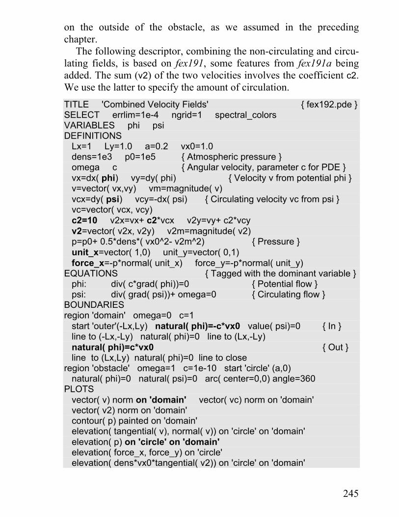
Combined Velocity Fields

In order to obtain a more general solution for irrotational liquid flowwe add a circulating field to the potential field from fex182. Aconvenient way of adding these fields is to calculate both by the samedescriptor. We are perfectly free to solve for φ and ψsimultaneously, but the solution domains must be identical.Unfortunately, the potential field had a void for the obstacle, whilethe domain for the circulating velocity field was defined over a theentire square without an excluded region.

In order to solve for φ over the full domain, we may use a PDEthat is slightly different from p.226 1, i.e.

∂∂

∂∂

φ( ) ( ) ( ) ( )cvx

cvy

c cx y+ ≡ ∇⋅ = ∇ ⋅ ∇ =v 0

The idea is to define the constant c to be unity in the liquid and totake a suitably small value co in the region of the obstacle. The FEAprogram arranges to make the normal component ( )c nv continuousacross the interface from obstacle to liquid. This means that therelation 1⋅ =v c vn o on will make vn on the liquid side much smallerthan v in the region of the obstacle, which in turn is of the order ofthe input speed. In other words, the velocity will be closely tangential

245

on the outside of the obstacle, as we assumed in the precedingchapter.

The following descriptor, combining the non-circulating and circu-lating fields, is based on fex191, some features from fex191a beingadded. The sum (v2) of the two velocities involves the coefficient c2.We use the latter to specify the amount of circulation.TITLE 'Combined Velocity Fields' { fex192.pde }SELECT errlim=1e-4 ngrid=1 spectral_colorsVARIABLES phi psi DEFINITIONS Lx=1 Ly=1.0 a=0.2 vx0=1.0 dens=1e3 p0=1e5 { Atmospheric pressure } omega c { Angular velocity, parameter c for PDE } vx=dx( phi) vy=dy( phi) { Velocity v from potential phi } v=vector( vx,vy) vm=magnitude( v) vcx=dy( psi) vcy=-dx( psi) { Circulating velocity vc from psi } vc=vector( vcx, vcy) c2=10 v2x=vx+ c2*vcx v2y=vy+ c2*vcy v2=vector( v2x, v2y) v2m=magnitude( v2) p=p0+ 0.5*dens*( vx0^2- v2m^2) { Pressure } unit_x=vector( 1,0) unit_y=vector( 0,1) force_x=-p*normal( unit_x) force_y=-p*normal( unit_y)EQUATIONS { Tagged with the dominant variable } phi: div( c*grad( phi))=0 { Potential flow } psi: div( grad( psi))+ omega=0 { Circulating flow } BOUNDARIESregion 'domain' omega=0 c=1 start 'outer'(-Lx,Ly) natural( phi)=-c*vx0 value( psi)=0 { In } line to (-Lx,-Ly) natural( phi)=0 line to (Lx,-Ly) natural( phi)=c*vx0 { Out } line to (Lx,Ly) natural( phi)=0 line to closeregion 'obstacle' omega=1 c=1e-10 start 'circle' (a,0) natural( phi)=0 natural( psi)=0 arc( center=0,0) angle=360PLOTS vector( v) norm on 'domain' vector( vc) norm on 'domain' vector( v2) norm on 'domain' contour( p) painted on 'domain' elevation( tangential( v), normal( v)) on 'circle' on 'domain' elevation( p) on 'circle' on 'domain' elevation( force_x, force_y) on 'circle' elevation( dens*vx0*tangential( v2)) on 'circle' on 'domain'

246

contour( curl( v2)) contour( div( v2))END

The following figure is a vector plot of the combined velocity v2. Itshows that the speed is now higher below the obstacle, as we mightexpect.

The plot below tests to what extent the normal velocity vanishes onthe circle.

247

The above plot shows that vn is in fact smaller than vt butfluctuates noticeably around zero. This is the best that can be done,however, with this limited number of nodes. Using the ProfessionalVersion with a smaller value of errlim we obtain less scatter and novisible net variation.

In order to calculate the force acting on the obstacle, we integrate− p n xcos( , ) over the circle to obtain the x-component of the force,and so on. In practice, we construct a unit vector field unit_x, whichcombines with normal to give us the direction cosine.

In this example, the pertinent velocity field exists in the liquidregion, which we have to keep in mind when plotting and calculatingline integrals. Under boundaries we first define a total domain andthen reserve a circular region for the obstacle. As a consequence ofthis definition, 'domain' becomes equivalent to the remainder, i.e. theliquid region.

For the line integrals, FlexPDE permits us to specify both the curvefor integration ('circle') and the region where the data are to befetched. We specify this by the modifier on 'circle' on 'domain'.

The elevation plot of the local forces shows that the integral offorce_x is now small compared to force_y, which takes a negativevalue (-1302). The force is thus perpendicular to the main stream anddirected downwards, as is also evident from the contour plot of thepressure.

Kutta and Joukovski8p156 used a complex formalism to derive anexpression for the force on a cylindrical object of general shape. Theresult for the lift force isF vy x= −ρ 0Γ

Judging from the last elevation plot, which yields the circulation (Γ),our integrated value agrees reasonably well with the analytic resultfor the negative lift force.

We have seen that the circulating mode of motion may produce aforce on the obstacle, transverse to the input velocity vx0. This issimilar to the Magnus effect8p159, which is easily observed in a tenniscourt. There is no drag force, however, on a cylinder in a non-viscousliquid.

248

Finally, the contour plots of div(v2) and curl(v2) confirm that thecombined velocity field conserves mass and is irrotational.

Forces on an Inclined Plate

Let us now apply the above PDEs to fex183 in the preceding chapter,exploiting suitable fractions of fex192. Here, we exploit the featurethat a boundary condition need not be repeated if unchanged.TITLE 'Forces on an Inclined Plate' { fex193.pde }SELECT errlim=1e-4 ngrid=1 spectral_colorsVARIABLES phi psi DEFINITIONS Lx=1.0 Ly=1.0 a=0.5*Ly d=0.2*a{ Geometric parameters for inclined plate } alpha=30* pi/180 { Angle of attack, radians } si=sin( alpha) co=cos( alpha) x1=-d/2*si- a/2*co y1=-d/2*co+ a/2*si { Corners } x2=d/2*si- a/2*co y2=d/2*co+ a/2*si x3=-x1 y3=-y1 x4=-x2 y4=-y2 dens=1e3 p0=1e5 { Atmospheric pressure at left end } vx0=5 vx=dx(phi) vy=dy(phi) { Velocity from potential phi } v=vector( vx, vy) vm=magnitude( v) unit_x=vector( 1,0) unit_y=vector( 0,1) omega c { Angular velocity and parameter for PDE } vcx=dy( psi) vcy=-dx( psi) { Circulating field from psi } vc=vector( vcx, vcy) vcm=magnitude( vc){ Combining velocities v and vc to obtain v2 } c2=-30 v2x=vx+ c2*vcx v2y=vy+ c2*vcy v2=vector( v2x, v2y) v2m=magnitude( v2) p2=p0+ 0.5*dens*( vx0^2- v2m^2) { Pressure } force_x=-p2*normal( unit_x) force_y=-p2*normal( unit_y)EQUATIONS { Tagged } phi: div( c*grad( phi))=0 { Potential flow } psi: div( grad( psi))+ omega=0 { Circulating flow }BOUNDARIESregion 'domain' omega=0 c=1 start 'outer' (-Lx,Ly) natural( phi)=-c*vx0 value( psi)=0 line to (-Lx,-Ly) { In } natural( phi)=0 line to (Lx,-Ly) natural( phi)=c*vx0 line to (Lx,Ly) { Out }

249

natural( phi)=0 line to closeregion 'obstacle' omega=1 c=1e-10 start 'rectangle' (x4,y4) natural( phi)=0 natural( psi)=0 line to (x3,y3) to (x2,y2) to (x1,y1) to closePLOTS vector( v) norm on 'domain' vector( vc) norm on 'domain' vector( v2) norm on 'domain' contour( p2) painted on 'domain' elevation( tangential( v), normal( v)) on 'rectangle' on 'domain' elevation( force_x, force_y) on 'rectangle' on 'domain' elevation( dens*vx0* tangential( v2)) on 'rectangle' on 'domain'END

The following vector plot indicates that the liquid flows along thesides of the plate as required. Since we now have chosen a negativevalue of c2, the combined velocity is higher on the top face of theplate, which we expect to result in a lift force.

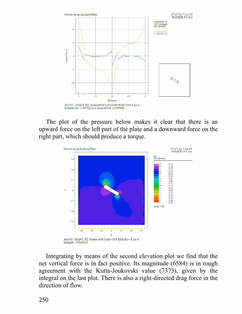
The following plot of vt and vn illustrates that the normal com-ponent is relatively small on the long sides, but that the few nodepoints on the short sides do not yield the ideal zero, but positive andnegative slopes.

250

The plot of the pressure below makes it clear that there is anupward force on the left part of the plate and a downward force on theright part, which should produce a torque.

Integrating by means of the second elevation plot we find that thenet vertical force is in fact positive. Its magnitude (6584) is in roughagreement with the Kutta-Joukovski value (7373), given by theintegral on the last plot. There is also a right-directed drag force in thedirection of flow.

251

In summary of this chapter, we note that an added circulating fieldreproduces to some extent the lift force found by experience. Therequired amount of circulation ( )Γ is not directly given by the Kutta-Joukovski theory, however, which means that the coefficient c2 has tobe determined by trial and error to provide smooth flow-off.

Most importantly, combining potential flow and circulating flowdoes not yield zero speed on the surface of the obstacle. This meansthat the detailed velocity field is unphysical, even if it predictsreasonable forces.

Exercises

Investigate if fex191 may be modified to accommodate an obstacleof square cross-section.

Explore how the lift and drag forces obtained by fex193 vary withthe angle of attack. What happens at negative alpha?

Adapt fex193 to treat flow around an obstacle of square cross-section.

252

20 Viscous Flow in Channels

In this chapter we shall deal with realistic situations in ( , )x y , where aliquid locally is at rest with respect to the solid objects in contact withit. Under such conditions curl(v) will in general be non-zero.

Classical mechanics applied to a liquid yields the Navier-Stokesequation8p59. That equation expresses Newton’s law of motion

ρ0ddt tot

v f=

for the total force ftot on a fluid element that is carried along with thestream. (That kind of derivative is also commonly denoted D Dv / t .)Here, ρ0 is the constant mass density of the fluid. Since the velocityin a chosen volume element is a function of ( , , )t x y , we may write

ddt t x

d xdt y

d ydt t

vx

vy tx y

v v v v v v v v v v= + + = + + = + ⋅∇∂∂

∂∂

∂∂

∂∂

∂∂

∂∂

∂∂

( )

With this expression for the derivative, Newton’s law takes the form

ρ ∂∂

ρ η0 02 0v v v F v

tp+ ⋅∇ − +∇ − ∇ =( )

where F is an external force (e.g. gravity), −∇p the force due topressure, and η∇2v the one proportional to viscosity8pp57,69. Thisvector PDE is known as the Navier-Stokes (N-S) equation.

The second term, ρ0 ( )v v⋅∇ , has the dimension of force but it isreally part of the time derivative and hence called an inertial force.This term is obviously second-order in v.

The last term corresponds to the viscous force on the volumeelement. Normally, ∇2 operates on a scalar and ∇2 v should be takenas shorthand for the vector ( )i j∇ + ∇2 2v vx y .

The simplest case of flow occurs at such small speeds that the non-linear inertial force become negligible compared to viscous force, and

253

in the present chapter we shall consider liquid motion under suchconditions. The ratio of inertial-to-viscous forces is usually expressedin the form of the dimensionless Reynolds number, defined by

Re = ρη

0 0 0v L

where v0 is a typical speed and L0 a typical size of the solutiondomain. This number gives us an order-of-magnitude indication ofthe sort of flow we are dealing with. At sufficiently small values ofRe, the inertial term is negligible compared to the viscous force andthe problem can be treated as linear in the dependent variables. ThePDEs then yield solutions corresponding to laminar flow.

Above the first critical value (Re )= 1 the solutions may remainlaminar, even if the PDEs are non-linear. Above a much higher value(Re=100 or much more depending of the details of the problem) thesolution becomes turbulent and time-dependent (permanentlyunstable).

In Cartesian coordinates, the component Navier-Stokes equationsmay thus be written (for the x- and y-directions respectively)

ρ

∂∂∂∂

ρ

∂∂∂∂

η

∂∂

∂∂

∂∂

∂∂

0 0

2

2

2

2

2

2

2

2

0

vt

vt

FF

pxpy

vx

vy

vx

vy

x

y

x

y

x x

y y

RS||

T||

UV||

W||+ ⋅∇ −

RSTUVW+

RS||

T||

UV||

W||−

+

+

RS||

T||

UV||

W||=( )v v

Here, we have kept the second term unexpanded, since it may bedisregarded until a later chapter.

So far, we have only two equations for the three dependentvariables vx , vy , and p. Conservation of mass at constant densitygives us a third equation8p52, i.e.

∇⋅ = ∇ ⋅ = +FHG

IKJ =( )ρ ρ ρ ∂

∂∂∂0 0 0 0v v v

xvy

x y

but unfortunately this is a PDE of first order only, which FlexPDEwould not accept.

254

Using ∇⋅ =v 0 together with the equation of motion we may,however, generate a relation containing second-order derivatives in p.Applying the divergence operator to the N-S equation we obtain11

ρ ∂∂

ρ η0 02 2 0

tp∇⋅ + ∇ ⋅ ⋅∇ −∇ ⋅ + ∇ − ∇⋅ ∇ =v v v F v( ) ( )

where the first term vanishes because of mass conservation.Furthermore, we may eliminate the last term using the identities

η η η∇⋅ ∇ = ∇ ∇⋅ = ∇ =( ) ( ) ( )2 2 2 0 0v v

The remainder of the modified N-S equation is

∇ + ∇⋅ ⋅∇ −∇⋅ =20 0p ρ ( )v v F

If the volume force F is constant in space the last term will vanish.Expressed in Cartesian coordinates, this PDE takes the form

∂∂

∂∂

ρ2

2

2

2 0 0px

py

+ + ∇ ⋅ ⋅∇ −∇⋅ =( )v v F

Even in this equation we leave the term containing ρ0 unexpanded,since it will not be used in the present chapter.

We now have a total of three PDEs for calculating vx , vy and p.Although we derived the equation for p using mass conservation, itwould be wrong to assume that any solution to these three PDEswould necessarily satisfy ∇⋅v=0. In fact, one may show11 that this istrue only in special cases. We shall see that the first two examples inthis chapter are sufficiently simple for the divergence to vanishautomatically.

It could never be wrong, however, to add ∇⋅v, multiplied by afactor, to the equation for p, since the divergence should vanish in thefinal stage of the solution process. Hence we settle for the followingform

∂∂

∂∂

ρ2

2

2

2 0 0px

py

f+ + ∇⋅ ⋅∇ −∇ ⋅ − ∇ ⋅ =∇( )v v F v

where we may choose the factor f∇ freely according to the problemat hand, to ensure vanishing divergence. Trial runs lead us to employ

255

a negative factor. We may always verify by means of plots that thedivergence vanishes for a given solution.

The factor f∇ may not be taken as a fixed number, however, sinceit has a physical dimension, in fact the same as η /L0

2 . Hence, weshould write

f CL∇ =η

02

where the parameter L0 is a typical size of the domain. The number Cis to be chosen empirically, large enough to ensure vanishing ∇⋅ v ,but not so large that it impairs convergence in FlexPDE calculationsor requires unreasonably long runtimes.

Although the divergence term was introduced on intuitive groundsand proves itself in practical use, we may understand approximatelyhow it works. In the derivation of p.252 1 we used the term f = −∇pfor the force generated by pressure. The Gauss theorem6p43 now yields

∇ = ∇⋅∇ = − ∇ ⋅ = −zzz zzz zzz zz2 pdV p dV dV f d snf

Let us now consider a small region around a point of interest. Bysubtracting a certain amount from the ∇2p term in p254 2 weeffectively create an outward force on the boundary of that region,which transports fluid away from the point considered. This nudgesthe calculations toward vanishing divergence.

Boundary Conditions

Now that we have a PDE for pressure, we must find out whatboundary conditions to use with it. This is easy enough where thepressure takes known values, but what about boundaries that just limitthe fluid flow?

The alternative to value is a natural statement. In the latter case weneed an expression for ∂ ∂p n p/ ≡ ⋅∇n , where n is the outwardnormal ( n = 1) at the boundary of the domain. The N-S equation(p.252) provides the answer rather directly11:

256

∇ = + ∇ − − ⋅∇pt

F v v v vη ρ ∂∂

ρ20 0 ( )

If the pressure is not known on a boundary segment, we may thus usethe following general expression for the natural boundary condition

∂ ∂ η ρ ∂∂

ρ

η ρ ∂∂

ρ

p n pt

n F n F n v n vtx x y y x x y y

/ ( )

( )

= ⋅∇ = ⋅ + ⋅∇ − ⋅ − ⋅ ⋅∇ =

+ + ∇ + ∇ − ⋅ − ⋅ ⋅∇

n n F n v n v n v v

n v n v v

20 0

2 20 0

where ρ ∂ ∂0 v tn / will vanish in the steady state, and we defer theexpansion of the last term until it is required later.

Steady Flow at Small Speeds (Re<<1)

In this chapter and the next one we shall only be concerned withsteady flow, which means that we omit the time derivative. We alsoassume Re to be small enough to permit us to neglect the PDE termproportional to the density. The three PDEs then take the simplerform

∂∂∂∂

η

∂∂

∂∂

∂∂

∂∂

pxpy

vx

vy

vx

vy

x x

y y

RS||

T||

UV||

W||−

+

+

RS||

T||

UV||

W||=

2

2

2

2

2

2

2

2

0

∂∂

∂∂

η ∂∂

∂∂

2

2

2

202 0p

xp

yC

Lvx

vy

x y+ − +FHG

IKJ =

We shall soon see that in the most elementary examples, involvingparallel flow, we may even neglect the last (divergence) term.

For small Re, the natural boundary condition for pressuresimplifies into∂ ∂ ηp n n F n F n v n vx x y y x x y y/ = + + ∇ + ∇2 2d i

257

Flow Due to a Moving Wall at Re<<1

We shall now consider the motion of a liquid confined between twoparallel walls. One wall is kept stationary and the other one moveswith speed vx0, at constant spacing between the walls. In order toobtain a small Reynolds number with the usual domain size andreasonable velocity, we have chosen a hypothetical liquid of veryhigh viscosity.

In the two preceding chapters we imposed the ambient pressure p0,because there was a risk of large negative pressures at corners,leading to voids. In the N-S PDE, only derivatives of p occur, andhence we may ignore p0 in the solution process. We may always addthe ambient pressure later to the solution for p to ensure that the totalpressure remains positive.

Under boundaries we specify the velocity components on the solidsurfaces. We assume that the moving wall, rather than a pressuredifference, drives the motion and hence the pressure is taken to bezero on both of the vertical sides. In the above expression for ∂ ∂p n/we have ny = 1 on the upper horizontal side, since the outwardnormal to the boundary points in the direction of positive y. On thelower boundary we must enter ny = −1.

TITLE 'Flow Due to a Moving Wall' { fex201.pde }SELECT errlim=1e-5 spectral_colors { Student Version }VARIABLES vx vy pDEFINITIONS Lx=1.0 Ly=1.0 vx0=1e-3 visc=1e4 { Viscosity } dens=1e3 Re=dens*vx0*2*Ly/visc { Reynolds number } v=vector( vx, vy) vm=magnitude( v) { Speed }EQUATIONS { Tagged by dominant variable } { For vanishing Re } vx: dx( p)- visc*div( grad( vx))=0 vy: dy( p)- visc*div( grad( vy))=0 p: div( grad( p))=0 { Divergence term neglected }BOUNDARIESregion 'domain' start 'outer' (-Lx,Ly) natural( vx)=0 value( vy)=0 value(p)=0 line to (-Lx,-Ly) { Left } value( vx)=0 value( vy)=0 natural(p)=-visc*div( grad( vy)) line to (Lx,-Ly) natural( vx)=0 value( vy)=0 value(p)=0 { Right } line to (Lx,Ly) value( vx)=vx0 value( vy)=0 { Upper }

258

natural(p)=visc*div( grad( vy)) line to closePLOTS elevation( vx, vy) on 'outer' report( Re) contour( vx) contour( vy) contour( p) vector( v) norm contour( div( v)) contour( curl( v)) paintedEND

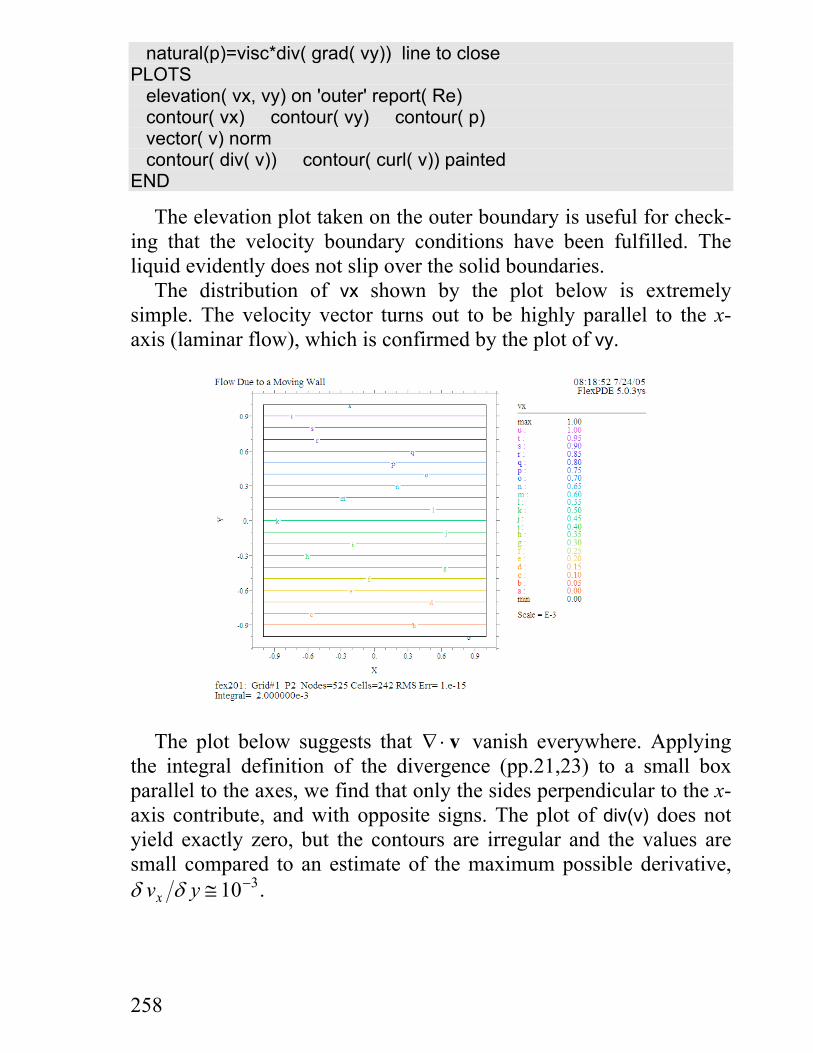
The elevation plot taken on the outer boundary is useful for check-ing that the velocity boundary conditions have been fulfilled. Theliquid evidently does not slip over the solid boundaries.

The distribution of vx shown by the plot below is extremelysimple. The velocity vector turns out to be highly parallel to the x-axis (laminar flow), which is confirmed by the plot of vy.

The plot below suggests that ∇⋅ v vanish everywhere. Applyingthe integral definition of the divergence (pp.21,23) to a small boxparallel to the axes, we find that only the sides perpendicular to the x-axis contribute, and with opposite signs. The plot of div(v) does notyield exactly zero, but the contours are irregular and the values aresmall compared to an estimate of the maximum possible derivative,δ δv yx ≅ −10 3.

259

Using the line integral definition of curl (p.21), we first notice thatits value must be the same everywhere. The local curl must thus equalthe average value we obtain from a line integral along the boundary,which amounts to ( ) / ( )0 2 2 20− ⋅v L L Lx x x y = − = − −v ex0 2 5 4/ . Thisresult is borne out by the plot of curl(v).

Pressure-Driven Flow through a Channel

As a second elementary example we study steady flow between twoparallel walls, driven by a prescribed pressure difference δp . Sincethe main velocity component will not be known beforehand, wecalculate the Reynolds number using globalmax, which yields thelargest value over the solution domain.

We shall use fex201 as a template for the following descriptor. Thenatural boundary conditions are equally simple in this case, since onlyny is non-zero on the solid boundaries. On the left and rightboundaries we specify natural(vx)=0, which means ∂ ∂v xx / = 0 on theend faces.

This problem has a simple analytic solution8p8, i.e.

v p w yx = −δ

η/l

22 2d i, vy = 0

260

where δp is the pressure difference between the ends, l the length ofthe channel, and 2w its width. Since vx is independent of x, thepressure gradient in that direction must be constant for symmetryreasons. The pressure p x( ) must thus be a linear function. This set offunctions may easily be shown to satisfy the PDEs and the boundaryconditions. We enter the expression for the horizontal velocity underthe notation vx_ex. The modifications to fex201 are as follows.TITLE 'Pressure-Driven Flow through a Channel' { fex202.pde }… Lx=1.0 Ly=1.0 visc=1e4 delp=100 { Driving pressure } vx_ex=delp/(2*Lx)/(2*visc)*(Ly^2- y^2) { Exact solution } dens=1e3 Re=dens*globalmax( vx)*2*Ly/visc…region 'domain' start 'outer' (-Lx,Ly) natural( vx)=0 value( vy)=0 value(p)=delp { In } line to (-Lx,-Ly) value( vx)=0 value( vy)=0 natural(p)=-visc*div( grad( vy)) line to (Lx,-Ly) natural( vx)=0 value( vy)=0 value(p)=0 { Out } line to (Lx,Ly) value( vx)=0 value( vy)=0 natural(p)=visc*div(grad( vy)) line to close… contour( vx- vx_ex) report( globalmax( vx))END

The plot below shows the solution for the horizontal component ofvelocity, vx. The value is zero at the horizontal boundaries and takes amaximum at mid-distance.

Comparing the contour plots of vx and vy we find that the velocityis accurately horizontal everywhere. This is another example oflaminar flow, and the simplicity of the motion makes it obvious thatdiv(v) must be zero.

261

The plot of the speed error (not shown here) indicates that vx istrue to about one part in 1012.

The plot below illustrates that curl(v) is non-zero everywhere,except in the symmetry plane, where this function changes sign.

We may also calculate the vorticity from the analytic solution as−∂ ∂v yx / . This is another example of innocent-looking, laminar flowthat proves to be rotational.

262

Viscous Flow through a Constricted Channel

The following is a modification of fex181, which should make it validfor viscous flow. Here, we have used the unit vector field which isexpedient for expressing the direction cosines ( , )n nx y occurring inthe natural boundary conditions for p. On the input and output faceswe have specified ∂ ∂v xx / = 0 , assuming that there is negligiblechange in vx close to the ends.

TITLE 'Viscous Flow through a Constricted Channel' { fex203.pde }SELECT errlim=1e-4 ngrid=1 spectral_colors VARIABLES vx vy pDEFINITIONS Lx=1.0 Ly=1.0 coef=0.5 visc=1e4 delp=100 { Driving pressure } dens=1e3 Re=dens*globalmax( vx)*2*Ly/visc v=vector( vx, vy) vm=magnitude( v) unit_x=vector(1,0) unit_y=vector(0,1) { Unit vector fields } nx=normal( unit_x) ny=normal( unit_y) {Direction cosines }{ Natural boundary condition for p: } natp=visc*[ nx*div( grad( vx))+ ny*div( grad( vy))]EQUATIONS vx: dx( p)- visc*div( grad( vx))=0 vy: dy( p)- visc*div( grad( vy))=0 p: div( grad( p))=0BOUNDARIESregion 'domain' start 'outer' (0,Ly) natural( vx)=0 value( vy)=0 value( p)=delp { In } line to (0,-Ly) value( vx)=0 value( vy)=0 natural( p)=natp line to (Lx,-Ly) to (2*Lx,-Ly*coef) to (3*Lx,-Ly*coef) natural( vx)=0 value( vy)=0 value( p)=0 { Out } line to (3*Lx,Ly*coef) value( vx)=0 value( vy)=0 natural( p)=natp line to (2*Lx,Ly*coef) to (Lx,Ly) to closePLOTS elevation( nx, ny) on 'outer' as 'direction cosines' contour( vx) report(Re) contour( vm) vector( v) norm contour( p) contour( div( v)) painted contour( curl( v)) painted elevation( vx) from (0.5*Lx,-Ly) to (0.5*Lx,Ly) elevation( vx) from (2.5*Lx,-Ly*coef) to (2.5*Lx,Ly*coef)END

263

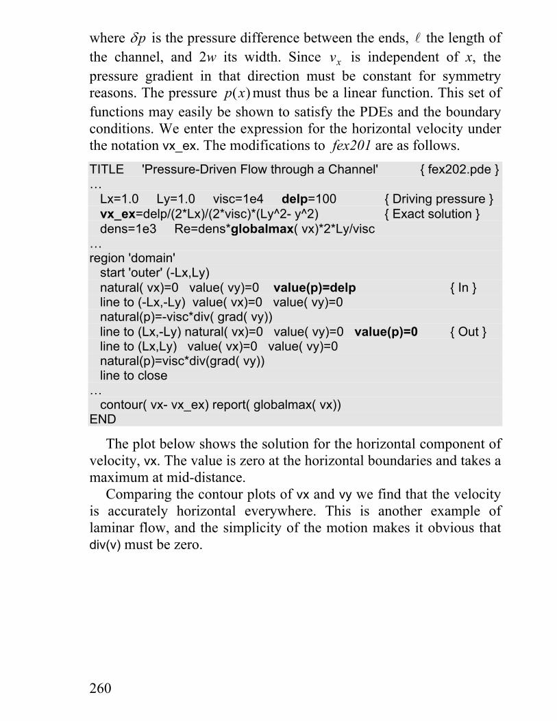
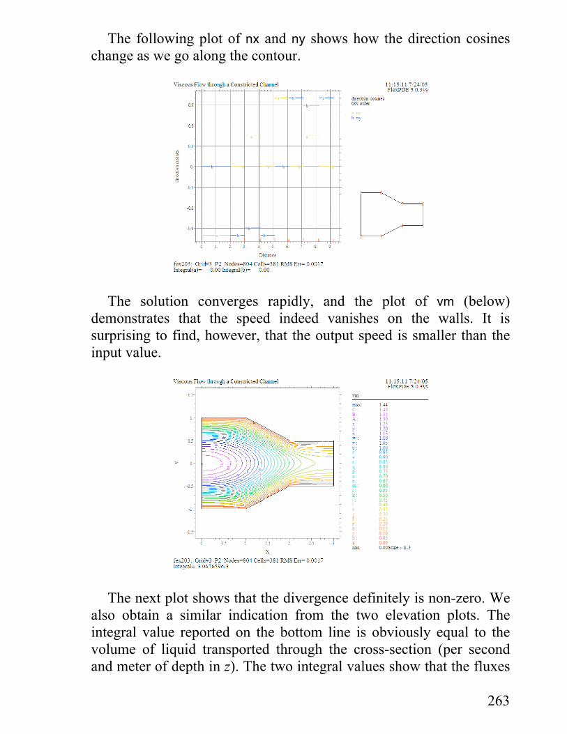
The following plot of nx and ny shows how the direction cosineschange as we go along the contour.

The solution converges rapidly, and the plot of vm (below)demonstrates that the speed indeed vanishes on the walls. It issurprising to find, however, that the output speed is smaller than theinput value.

The next plot shows that the divergence definitely is non-zero. Wealso obtain a similar indication from the two elevation plots. Theintegral value reported on the bottom line is obviously equal to thevolume of liquid transported through the cross-section (per secondand meter of depth in z). The two integral values show that the fluxes

264

through the cross-sections are different. In short, the solution does notconserve mass and is definitely wrong!

The cause of this discrepancy is that we have not yet used the extraterm in the 3rd PDE that was designed to suppress div(v).

Acting on the warning received, we now introduce the termcontaining div(v) in the last PDE of fex203. The numerical factor 1e4has been found suitable by trial and error.TITLE 'Constricted Channel with Divergence Term' { fex203a.pde }...EQUATIONS vx: dx( p)- visc*div( grad( vx))=0 vy: dy( p)- visc*div( grad( vy))=0 p: div( grad( p))- 1e4*visc/Lyˆ2*div(v)=0... contour( div( v)) elevation( natp) on 'outer'END

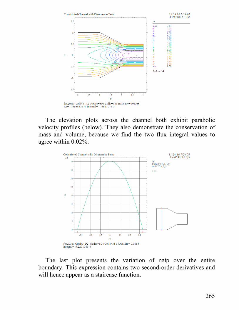
From the following plot of vx we notice that the maximum speed atthe exit now is about twice that at the entrance. The plot of div(v) nowexhibits the irregular contours that characterize a vanishing function.

265

The elevation plots across the channel both exhibit parabolicvelocity profiles (below). They also demonstrate the conservation ofmass and volume, because we find the two flux integral values toagree within 0.02%.

The last plot presents the variation of natp over the entireboundary. This expression contains two second-order derivatives andwill hence appear as a staircase function.

266

Comparison with Irrotational Flow

It might be interesting to compare viscous flow through a constrictedchannel with that pertaining to a velocity potential φ (p.226). In orderto bring the boundary conditions into closer agreement we change thespeed distribution at the input, such as to produce a parabolic velocityprofile. The definition of vx0 in fex181 needs to be modified, and weshould adapt the plots to the new situation.TITLE 'Constricted Channel, Parabolic vx0' { fex181a.pde }... vx0=4.0e-4*(Ly^2- y^2)/Ly^2 { Velocity at input end }...PLOTS elevation( vx0) from (0,-Ly) to (0,Ly) elevation( vx) from (Lx/2,-Ly) to (Lx/2,Ly) elevation( vx) from (3*Lx,-Ly) to (3*Lx,Ly) vector( v) norm contour( vx) painted contour( vm) painted contour( div(v)) contour( curl(v))END

267

The elevation plots illustrate that the initially parabolic distributionchanges and finally becomes nearly flat at the end, in contrast to whatwe observed in fex203a. The following vector plot confirms this.

This example shows that the behavior of viscous flow isdramatically different from that of potential flow. It is possible,however, to consider viscous flow through a channel as potential flowin a region sufficiently far from the walls. The region close to thewall, where the vorticity is large (the boundary layer), may be treatedseparately.

Tangential Input Velocity

We now return to an example involving a rectangular domain. Here,we specify a constant vertical velocity vy0 at the left face, whilekeeping the other three sides closed by fixed walls. In practice, wecould impose this lateral velocity by an endless tape, driven overrollers at constant velocity past the left face. The template for thisexample is fex203a.TITLE 'Tangential Input Velocity' { fex204.pde }SELECT errlim=1e-4 ngrid=1 spectral_colorsVARIABLES vx vy pDEFINITIONS Lx=1.0 Ly=1.0 visc=1.0

268

vy0=1e-5 { Input velocity } dens=1e3 Re=dens*globalmax( vx)*2*Ly/visc v=vector( vx, vy) vm=magnitude( v) unit_x=vector(1,0) unit_y=vector(0,1) { Unit vector fields } nx=normal( unit_x) ny=normal( unit_y) { Direction cosines } natp=visc*[ nx*div( grad( vx))+ ny*div( grad( vy))]EQUATIONS vx: dx( p)- visc*div( grad( vx))=0 vy: dy( p)- visc*div( grad( vy))=0 p: div( grad( p))- 1e4*visc/Lyˆ2*div( v)=0BOUNDARIESregion 'domain' start 'outer' (-Lx,-Ly) value( vx)=0 value( vy)=0 natural(p)=natp line to (Lx,-Ly) to (Lx,Ly) to (-Lx,Ly) value( vx)= 0 value( vy)=vy0 line to closePLOTS vector( v) norm report(Re) contour( vm) contour( p) contour( div( v)) contour( curl( v)) paintedEND

We again exploit a convenient feature of FlexPDE that makes anyboundary condition valid for the following segments, until modified.For instance, natp need not be repeated for each of the sides.

The above vector plot displays a kind of circulation, centered on apoint not far from the left face. This is not circulation in the sense ofthe preceding chapter, however, because another plot shows that

269

curl(v) is definitely non-zero. In fact, the vorticity appears to takeopposite signs in different regions.

The contour plot of div(v) yields the irregular contours of valuezero that we usually associate with a vanishing function.

Channel with a Lateral Cavity

In fex202, the channel walls assured parallel flow. Let us now studythe case of a channel provided with a lateral cavity as shown in thenext figure. We keep a few lines from the descriptor fex204 andmodify the others as follows.

Under boundaries, five line segments will have equal boundaryconditions, and hence we may simplify by specifying those only once.TITLE 'Channel with a Lateral Cavity' { fex205.pde }…DEFINITIONS Lx=1.0 Ly=1.0 visc=0.1 delp=1e-6 { Replaces vy0 }...region 'domain' start 'outer' (0,Ly) natural(vx)=0 value( vy)=0 value(p)=delp { In } line to (0,0) value(vx)=0 value(vy)=0 natural(p)=natp line to (Lx,0) to (Lx,-Ly) to (2*Lx,-Ly) to (2*Lx,0) to (3*Lx,0) natural(vx)= 0 value(p)=0 line to (3*Lx,Ly) { Out } value(vx)= 0 natural(p)=natp line to closePLOTS vector( v) norm report( Re) contour( vm) vector( v) norm zoom(Lx,-Ly, Lx,Ly) contour( p) contour( div( v)) contour( curl(v)) painted elevation( vx) from (0.5*Lx,0) to (0.5*Lx,Ly) elevation( vx) from (1.5*Lx,-Ly) to (1.5*Lx,Ly) elevation( vx) from (2.5*Lx,0) to (2.5*Lx,Ly)END

The plot of vm below shows that the flow is mainly confined to thethrough part of the channel, the velocity being much lower in theadjacent cavity. Clearly, this plot is symmetric with respect to theplane x = 1 5. .

270

Both vector plots demonstrate that circulation occurs in the cavity,and the curl is again non-zero. The plot below clearly shows thecenter of circulation.

The plot of div(v) demonstrates that the solution is compatible withmass and volume conservation. In particular, the three elevation plotsacross the channel quantitatively confirm that no mass is lost alongthe stream.

271

Uniform Velocity of Injection

So far we have injected fluid into a channel at uniform pressure. Analternative would be to impose uniform input velocity, resulting in anon-uniform pressure distribution over the input area. We shall nowsolve this problem for the constricted channel (fex203).

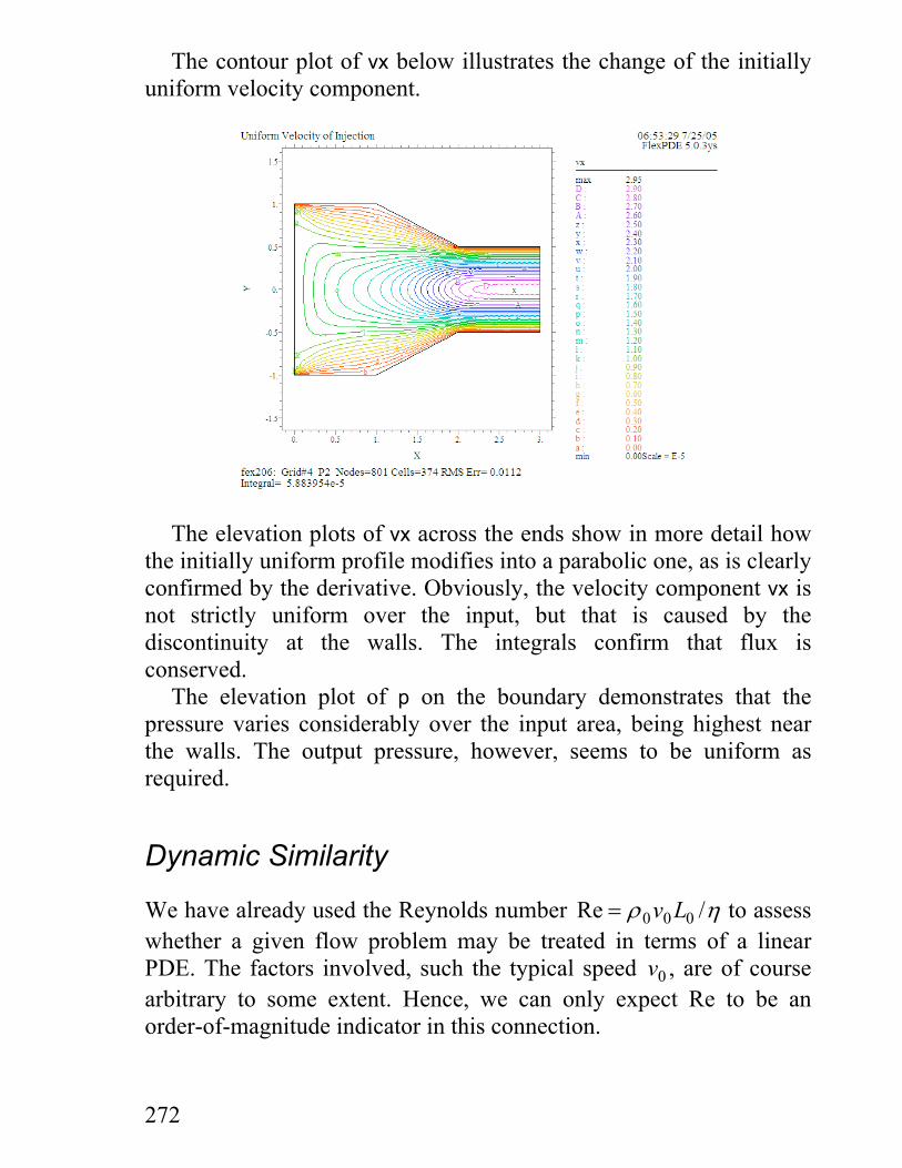
The boundary conditions for pressure are by derivatives (natural),except at the exit where we specify the value p = 0. To obtain thetotal pressure we just add the ambient value. We now modify fex204to obtain the following file.TITLE 'Uniform Velocity of Injection' { fex206.pde }SELECT errlim=1e-3 ngrid=1 spectral_colorsVARIABLES vx vy p { Pressure minus ambient }DEFINITIONS Lx=1.0 Ly=Lx coef=0.5 visc=1.0 vx0=1e-5 { Input velocity } dens=1e3 Re=dens*vx0*2*Ly/visc v=vector( vx, vy) vm=magnitude( v) unit_x=vector(1,0) unit_y=vector(0,1) { Unit vector fields } nx=normal( unit_x) ny=normal( unit_y) {Direction cosines } natp=visc*[ nx*div( grad( vx))+ ny*div( grad( vy))]EQUATIONS vx: dx( p)- visc*div( grad( vx))=0 vy: dy( p)- visc*div( grad( vy))=0 p: div( grad( p))- 1e4*visc/Lyˆ2*div( v)=0BOUNDARIESregion 'domain' start 'outer' (0,Ly) value( vx)=vx0 natural( vy)=0 natural( p)=natp { In } line to (0,-Ly) value( vx)=0 value( vy)=0 natural( p)=natp line to (Lx,-Ly) to (2*Lx,-Ly*coef) to (3*Lx,-Ly*coef) { Wall } natural( vx)=0 natural( vy)=0 value( p)=0 { Out } line to (3*Lx,Ly*coef) value( vx)=0 value( vy)=0 natural( p)=natp line to (2*Lx,Ly*coef) to (Lx,Ly) to close { Wall }PLOTS elevation( vx) from (0,-Ly) to (0,Ly) elevation( vx, 0.1*dy( vx)) from (3*Lx,-Ly*coef) to (3*Lx,Ly*coef) elevation( p) on 'outer' vector( v) norm report(Re) contour( vx) contour( vy) contour( vm) contour( p) contour( div( v)) contour( curl( v)) paintedEND

272

The contour plot of vx below illustrates the change of the initiallyuniform velocity component.

The elevation plots of vx across the ends show in more detail howthe initially uniform profile modifies into a parabolic one, as is clearlyconfirmed by the derivative. Obviously, the velocity component vx isnot strictly uniform over the input, but that is caused by thediscontinuity at the walls. The integrals confirm that flux isconserved.

The elevation plot of p on the boundary demonstrates that thepressure varies considerably over the input area, being highest nearthe walls. The output pressure, however, seems to be uniform asrequired.

Dynamic Similarity

We have already used the Reynolds number Re = ρ η0 0 0v L / to assesswhether a given flow problem may be treated in terms of a linearPDE. The factors involved, such the typical speed v0 , are of coursearbitrary to some extent. Hence, we can only expect Re to be anorder-of-magnitude indicator in this connection.

273

Another application of Re is to exploit knowledge gained fromcalculation or experiment to predict the flow in an enlarged orreduced geometry – still at the same value of Re. Here, the predictionis accurate, as we shall see.

To reveal the similarity between situations characterized by agiven value of Re, we start from the N-S vector equation. (Theadditional equation (p.254 1) only arranges to make ∇⋅ =v 0 andneed not concern us here.) We thus consider the PDE

ρ ∂∂

ρ η0 02 0v v v F v

tp+ ⋅∇ − +∇ − ∇ =( )

The key to the prediction is a transformation of the variables intonon-dimensional form. The new (primed) variables may be expressedas follows.t t v L' /= 0 (time) r r' /= L (position) v v' /= v0 (velocity)

p p v' /( )= ρ0 02 (pressure) F F' /( / )= ρ0 0

2v L ( volume force )

The new variables t ' , r' , and v' are obviously non-dimensional,but the reference length L and speed v0 must be identically defined inthe problems to be compared. For instance, we might choose themaximum value of the variable, or the value for a point at the middleof the stream. The actual values, however, would be different.

All five terms in the above N-S equation have the same dimension.Comparing the second and fourth terms we see that (dimensionally)

ρ ν0

02

LpL

⇔

and hence that ρ0 02v must have the same dimension as p. Of course,

you can also see this by expanding the dimensional expressions.A similar comparison of the third and fourth terms leads us to an

expression for the non-dimensional variable F' .Applying the above transformations we obtain the non-

dimensional form for the N-S equation.

ρ ∂∂

ρ ρ ρ η00

00

02

0 02

0 02

02

2 0vL v t

vL

vL

vL

p vL/

''

( ' ) ' ' ' 'v v v F v+ ⋅∇ − + ∇ − ∇ =

274

Multiplying through by L v/( )ρ0 02 gives us the simpler PDE

∂∂

v v v F v''

( ' ) ' ' 'Re

't

p+ ⋅∇ − +∇ − ∇ =1 02

From this it is clear that the solution in terms of primed variables onlydepends on the value of Re, if the boundary conditions are the same.Knowing the solution to one such problem we can thus generatesolutions to an infinite number of problems having the same value ofRe.

Let us now explore whether two problems with similar boundaryconditions and proportional geometric dimensions have the sameprimed solutions. We first modify fex206 to display the primedvariables, using vx0 and Lx as reference values. We need nottransform x and y, since the geometrical factors will be reducedautomatically on plotting. In anticipation we also calculate the meanvalue of v' (vpm) to facilitate comparison.

TITLE 'Dynamic Similarity' { fex206a.pde }… { Primed variables: } vxp=vx/vx0 vyp=vy/vx0 vp=vector( vxp, vyp) vpm=magnitude( vp) pp=p/(dens*vx0^2) area=area_integral(1) vpm_mean=area_integral( vpm)/areaEQUATIONS…PLOTS vector( vp) norm report(Re) contour( vpm) report(vpm_mean) contour( pp) contour( abs( pp)/area)END

We are now ready to compare to a problem with other parameters.Since Re depends on four quantities, we must change at least two ofthem to produce the same value. In the following descriptor, based onfex206a, we modify three factors.TITLE 'Dynamic Similarity, Other Parameters' { fex206b.pde }… Lx=0.1 Ly=Lx coef=0.5 visc=0.01 vx0=1e-6…

If we make both scripts show the plots, enlarging the second plotof each, we may compare corresponding figures quickly by clicking

275

on the tabs at the top. We can then proceed similarly with the otherplots.

We find that the following plot reports the same mean value for themagnitude vpm to five digits. It is possible to transform back tounprimed variables in order to obtain results in the usual form.

From the third plot it appears that pp varies over the same range inthe two descriptors. In order to make a more accurate comparison, wecould integrate the results. Considering that the geometrical sizes aredifferent (by a factor of 100), we should also divide by the area toobtain mean values. These also turn out to be nearly equal.

We finally note that the dimensional expression for the ratio of theinertial-to-viscous terms is

ρη

ρη

02

0 02

0

0 02

( ) //

Rev vv⋅∇

∇≅ =

v Lv L

which means that Re is a rough measure of the importance of the non-linear term in the PDE.

276

Exercises

Show analytically that the function vx_ex (p.260) satisfies thePDEs and the boundary conditions.

Verify the numeric calculation of curl(v) in fex202 using thefunction vx_ex.

Modify fex203a such as to produce a sudden constriction at x Lx= . Modify fex203a to produce a sudden widening of the channel at

x Lx= . Use Ly=0.4 and coef=2.0. Explore the results of fex206 using coef=1.0 and coef=2.0. Repeat

the solution for Lx=2.0. Create circular constrictions on the channel in fex205 as indicated

by the figure below. Let the minimum channel width be 0.2.

277

21 Viscous Flow past an Obstacle

We shall now study slow viscous flow in a channel containing anobstacle. The practical difference with respect to the precedingchapter is that we shall have to exclude a region corresponding to theobstacle and specify boundary conditions on its surface.

Viscous Flow past a Circular Cylinder

Here, we revisit an example from the chapter on irrotational flow(fex182, p.231). We need to add the PDEs for viscous flow and thepertinent boundary conditions, using the convenient formulation for ageneral orientation (natp) from fex203.

Empirically it has been found that natp=0 often is a sufficientlygood approximation to the full expression, at least for Re<<1. In thenext example we test this simplification by successive runs, using thestages device. The program sets the parameter stage to be 1 in thefirst run and 2 in a second run, where we use the full natp.TITLE 'Viscous Flow past a Circular Cylinder' { fex211.pde }SELECT errlim=1e-3 ngrid=1 spectral_colors stages=2VARIABLES vx vy pDEFINITIONS Lx=2.0 Ly=1.0 a=0.2 visc=1e4 delp=100 { Driving pressure } dens=1e3 Re=dens*globalmax( vx)*2*Lx/visc v=vector( vx, vy) vm=magnitude( v) unit_x=vector(1,0) unit_y=vector(0,1) { Unit vector fields } nx=normal( unit_x) ny=normal( unit_y) { Direction cosines } natp= if stage=2 then visc*[ nx*div( grad( vx))+ ny*div( grad( vy))] else 0EQUATIONS vx: dx( p)- visc*div( grad( vx))=0 vy: dy( p)- visc*div( grad( vy))=0 p: div( grad( p))- 1e4*visc/Lyˆ2*div( v)=0

278

BOUNDARIESregion 'domain' start 'outer' (-Lx,Ly) natural( vx)=0 natural( vy)=0 value(p)=delp { In } line to (-Lx,-Ly) value( vx)=0 value( vy)=0 natural(p)=natp { Wall} line to (Lx,-Ly) natural( vx)=0 natural( vy)=0 value(p)=0 { Out } line to (Lx,Ly) value( vx)=0 value( vy)=0 natural(p)=natp { Wall } line to close start 'outline' (a,0) { Exclude cylinder } value( vx)=0 value( vy)=0 natural(p)=natp arc( center=0,0) angle=360 closePLOTS contour( vx) report( Re) contour( vy) contour( vm) painted contour( p) vector( v) norm vector(v) norm zoom(-2*a,-2*a, 4*a,4*a) contour( div( v)) contour( curl( v)) painted elevation( vx, vy) from (-Lx,0) to (Lx,0)END

The program runs the script in two stages. By clicking onFile,View we may easily compare the results with natp=0 to thoseexploiting the full expression for natp. We only need to select the twoplots and then switch from one to the other by means of Ctrl-Shift n(for next) and Ctrl-Shift b (for back).

The following plot for stage=2 illustrates that the speed vanisheson the solid surfaces and that the maximum speed occursapproximately midway between the cylinder and the wall.

279

Switching between stages 1 and 2 we find no visible change of thecontours of vx, and the integral values differ only in the fourthdecimal. The variation is about as small for vm and p. For the rest ofthe examples in this chapter we shall thus replace natp by 0 on thebasis of experience.

The information contained here and in the vector plots indicatesthat the flow is symmetric with respect to y = 0. Thus, there is nocirculation of the liquid around the obstacle.

In addition, the above plot suggests that the speed is symmetricwith respect to x = 0, as also appears from the two vector plots of v.The final elevation plot illustrates this symmetry in more detail.

The next figure illustrates the pressure field. We notice that thereare high values on the front side of the obstacle and negative valueson the rear side. The effect of this is to create a pressure force on theobstacle, in addition to viscous drag.

To the above pressure values we may add the ambient pressure(1e5), which makes the total pressure positive everywhere.

280

Viscous Force on a Solid Surface

In order to gain deeper insight, we shall consider the forces on thewalls and on a solid cylinder in the channel. In an earlier chapter(p.245) we only calculated the force due to pressure, but we must nowinclude the effects of viscosity. For a solid surface perpendicular tothe y-axis, the definition of viscosity directly gives us the viscousforce per unit area8p4, i.e.

f vyxx= η ∂

∂

For a solid surface of arbitrary orientation we may write the tangentialforce per unit area as

f vntt= η ∂

∂

With v v t v tt x x y y= ⋅ = +v t , where t is the tangential unit vector, weobtain the general expression

f vn

vn

tvn

ttt x

xy

y= = +FHG

IKJη ∂

∂η ∂

∂∂∂

or after expanding the derivatives

f vx

xn

vy

yn

t vx

xn

vy

yn

ttx x

xy y

y= +FHG

IKJ + +FHG

IKJ

RSTUVW

η ∂∂

∂∂

∂∂

∂∂

∂∂

∂∂

∂∂

∂∂

f vx

n vy

n t vx

n vy

n ttx

xx

y xy

xy

y y= +FHG

IKJ + +FHG

IKJ

RSTUVW

η ∂∂

∂∂

∂∂

∂∂

where we have used the components of the normal unit vector n. Forthe Cartesian components of this force per unit area we obtainf f tx t x= , f f ty t y=

After having developed the expressions required, we now return tothe example of the circular cylinder to explore the forces caused bythe flow.

281

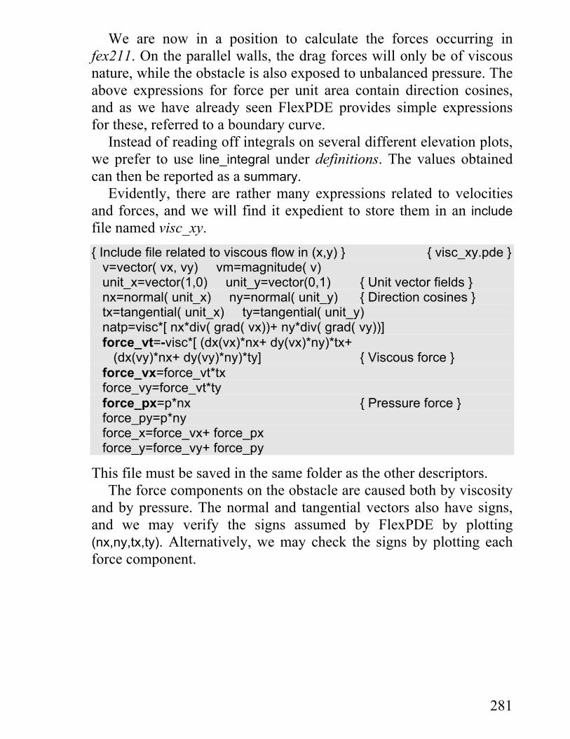
We are now in a position to calculate the forces occurring infex211. On the parallel walls, the drag forces will only be of viscousnature, while the obstacle is also exposed to unbalanced pressure. Theabove expressions for force per unit area contain direction cosines,and as we have already seen FlexPDE provides simple expressionsfor these, referred to a boundary curve.

Instead of reading off integrals on several different elevation plots,we prefer to use line_integral under definitions. The values obtainedcan then be reported as a summary.

Evidently, there are rather many expressions related to velocitiesand forces, and we will find it expedient to store them in an includefile named visc_xy.{ Include file related to viscous flow in (x,y) } { visc_xy.pde } v=vector( vx, vy) vm=magnitude( v) unit_x=vector(1,0) unit_y=vector(0,1) { Unit vector fields } nx=normal( unit_x) ny=normal( unit_y) { Direction cosines } tx=tangential( unit_x) ty=tangential( unit_y) natp=visc*[ nx*div( grad( vx))+ ny*div( grad( vy))] force_vt=-visc*[ (dx(vx)*nx+ dy(vx)*ny)*tx+ (dx(vy)*nx+ dy(vy)*ny)*ty] { Viscous force } force_vx=force_vt*tx force_vy=force_vt*ty force_px=p*nx { Pressure force } force_py=p*ny force_x=force_vx+ force_px force_y=force_vy+ force_py

This file must be saved in the same folder as the other descriptors.The force components on the obstacle are caused both by viscosity

and by pressure. The normal and tangential vectors also have signs,and we may verify the signs assumed by FlexPDE by plotting(nx,ny,tx,ty). Alternatively, we may check the signs by plotting eachforce component.

282

Forces on a Circular Cylinder

Let us now introduce the above commands into fex211 and calculatethe various force components. Here, we employ the standard name'outline' for the contour of the obstacle.TITLE 'Flow past a Circular Cylinder, Forces' { fex211a.pde }SELECT errlim=1e-3 ngrid=1 spectral_colorsVARIABLES vx vy pDEFINITIONS Lx=2.0 Ly=1.0 a=0.2 visc=1e4 delp=100 { Driving pressure } dens=1e3 Re=dens*globalmax( vx)*2*Lx/visc#include 'visc_xy.pde' F_wall_x=line_integral( force_vx,'outer') { Force on walls } F_vx=line_integral( force_vx,'outline') { Viscous force } F_px=line_integral( force_px,'outline') { Pressure force } F_x=line_integral( force_x,'outline') { Sum of x-forces } F_vy=line_integral( force_vy,'outline') { Viscous force } F_py=line_integral( force_py,'outline') { Pressure force } F_y=line_integral( force_y,'outline') { Sum of y-forces }EQUATIONS vx: dx( p)- visc*div( grad( vx))=0 vy: dy( p)- visc*div( grad( vy))=0 p: div( grad( p))- 1e4*visc/Lyˆ2*div( v)=0BOUNDARIESregion 'domain' start 'outer' (-Lx,Ly) natural( vx)=0 natural( vy)=0 value(p)=delp { In } line to (-Lx,-Ly) value( vx)=0 value( vy)=0 natural(p)=0 { natp=0 } line to (Lx,-Ly) natural( vx)=0 natural( vy)=0 value(p)=0 { Out } line to (Lx,Ly) value( vx)=0 value( vy)=0 natural(p)=0 { natp=0 } line to close start 'outline' (a,0) { Exclude } value( vx)=0 value( vy)=0 natural(p)=0 { natp=0 } arc( center=0,0) angle=360 closePLOTS contour( vx) report( Re) elevation( force_vx) on 'outline'summary report(F_wall_x) report( F_vx) report( F_px) report(F_x) report( F_vy) report( F_py) report(F_y)END

283

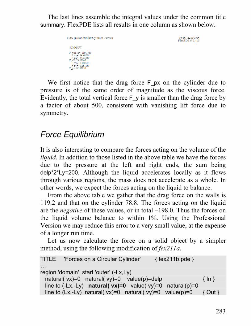
The last lines assemble the integral values under the common titlesummary. FlexPDE lists all results in one column as shown below.

We first notice that the drag force F_px on the cylinder due topressure is of the same order of magnitude as the viscous force.Evidently, the total vertical force F_y is smaller than the drag force bya factor of about 500, consistent with vanishing lift force due tosymmetry.

Force Equilibrium

It is also interesting to compare the forces acting on the volume of theliquid. In addition to those listed in the above table we have the forcesdue to the pressure at the left and right ends, the sum beingdelp*2*Ly=200. Although the liquid accelerates locally as it flowsthrough various regions, the mass does not accelerate as a whole. Inother words, we expect the forces acting on the liquid to balance.

From the above table we gather that the drag force on the walls is119.2 and that on the cylinder 78.8. The forces acting on the liquidare the negative of these values, or in total –198.0. Thus the forces onthe liquid volume balance to within 1%. Using the ProfessionalVersion we may reduce this error to a very small value, at the expenseof a longer run time.

Let us now calculate the force on a solid object by a simplermethod, using the following modification of fex211a.TITLE 'Forces on a Circular Cylinder' { fex211b.pde }…region 'domain' start 'outer' (-Lx,Ly) natural( vx)=0 natural( vy)=0 value(p)=delp { In } line to (-Lx,-Ly) natural( vx)=0 value( vy)=0 natural(p)=0 line to (Lx,-Ly) natural( vx)=0 natural( vy)=0 value(p)=0 { Out }

284

line to (Lx,Ly) natural( vx)=0 value( vy)=0 natural(p)=0 line to close…

The difference is that we now specify essentially slip (natural)boundary conditions on the walls. This increases the average speedand reduces the viscous force on the wall to negligible proportions.We thus expect the drag force on the object to balance the pressureforce on the liquid domain.

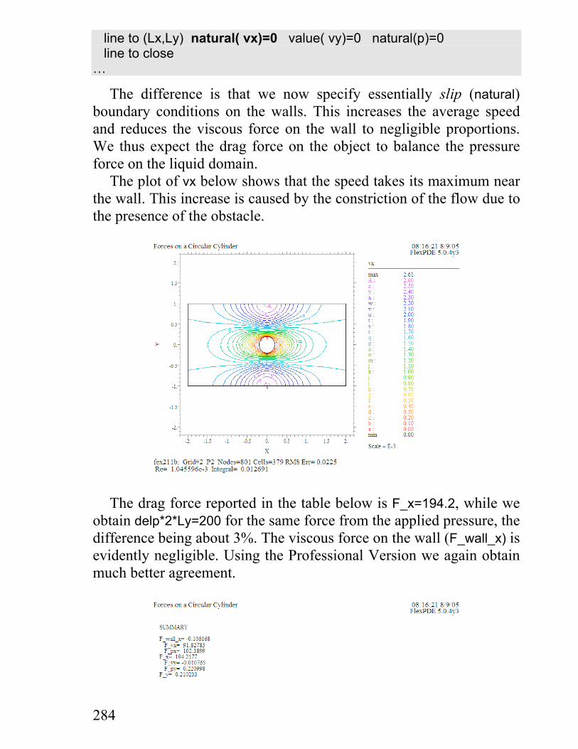
The plot of vx below shows that the speed takes its maximum nearthe wall. This increase is caused by the constriction of the flow due tothe presence of the obstacle.

The drag force reported in the table below is F_x=194.2, while weobtain delp*2*Ly=200 for the same force from the applied pressure, thedifference being about 3%. The viscous force on the wall (F_wall_x) isevidently negligible. Using the Professional Version we again obtainmuch better agreement.

285

Viscous Dissipation

Motion in a viscous medium involves internal friction that willgenerate heat. From an expression for the rate of change of kineticenergy and the N-S equation one obtains8p193,9p153 for the dissipatedpower per unit volume

P vk

vk

vid

i

ik

i k= +FHG

IKJ∑η ∂

∂∂∂

∂∂

where i and k are understood to run through the symbols x and y. Inexplicit form this sum expands into

P vx

vy

vx

vy

vx

vyd

x x y x y y=FHGIKJ +FHGIKJ +FHGIKJ + +

FHGIKJ

RS|T|

UV|W|

η ∂∂

∂∂

∂∂

∂∂

∂∂

∂∂

2 2 22 2 2 2

P vx

vy

vx

vyd

x x y y=FHGIKJ + +FHG

IKJ +FHGIKJ

RS|T|

UV|W|

η ∂∂

∂∂

∂∂

∂∂

2 22 2 2

The following descriptor, which is a modified fex211a, exploresthe energy balance by comparing the dissipated power with the rate ofwork done at the entrance.TITLE 'Flow past a Circular Cylinder, Dissipation' { fex211c.pde }… P_diss=visc*[2*dx(vx)^2+ (dy(vx)+ dx(vy))^2+ 2*dy(vy)^2]EQUATIONS…PLOTS contour( vm) painted contour( P_diss) elevation( vx*p) from (-Lx,Ly) to (-Lx,-Ly)END

The following plot shows that the dissipated power is largest onthe solid surfaces and close to the speed maximum, which could beexpected.

286

The elevation plot below permits us to compare this dissipatedpower (0.0685 per unit length in z) with the expended work (0.0669)on driving the liquid through the channel. The integral values for therates of dissipated energy and work evidently agree rather well.

287

Drag and Lift on an Inclined Plate

Having developed formalisms for forces we can now extend theanalysis to an inclined plate, combining features of fex193 andfex211b. The elevation plot on p.249 suggests that the expressions forthe force components, involving derivatives of vx and vy, would bedifficult to integrate because of the sharp corners. Hence, we preferthe boundary force formalism, based on the integrated force on theliquid volume.TITLE 'Drag and Lift on an Inclined Plate' { fex212.pde }SELECT errlim=1e-3 ngrid=1 spectral_colorsVARIABLES vx vy pDEFINITIONS Lx=1.0 Ly=1.0 a=0.5 d=0.1 visc=1.0{ Geometric parameters for inclined plate } alpha=30* pi/180 { Angle of attack, radians } si=sin( alpha) co=cos( alpha) x1=-d/2*si- a/2*co y1=-d/2*co+ a/2*si x2=d/2*si- a/2*co y2=d/2*co+ a/2*si x3=-x1 y3=-y1 x4=-x2 y4=-y2 delp=1e-5 { Driving pressure } dens=1e3 Re=dens*globalmax( vx)*2*Lx/visc#include 'visc_xy.pde'EQUATIONS vx: dx( p)- visc*div( grad( vx))=0 vy: dy( p)- visc*div( grad( vy))=0 p: div( grad( p))- 1e4*visc/Lyˆ2*div( v)=0BOUNDARIESregion 'domain' start 'outer' (-Lx,Ly) natural( vx)=0 natural( vy)=0 value(p)=delp { In } line to (-Lx,-Ly) natural( vx)=0 value( vy)=0 natural(p)=0 line to (Lx,-Ly) natural( vx)=0 natural( vy)=0 value(p)=0 { Out } line to (Lx,Ly) natural( vx)=0 value( vy)=0 natural(p)=0 line to close start 'outline' (x1,y1) { Exclude } value( vx)=0 value( vy)=0 natural(p)=0 line to (x2,y2) to (x3,y3) to (x4,y4) to closePLOTS contour( vx) report( Re) contour( vm) painted vector( v) norm contour( p) painted elevation( visc*dy( vx)) from (-Lx,-Ly) to (Lx,-Ly) { Fx on ''wall'' }

288

elevation( p) from (-Lx,-Ly) to (Lx,-Ly) { Force_y on liquid } elevation( p) from (-Lx,Ly) to (Lx,Ly) elevation( -p*normal( unit_y)) on 'outer' { Total Fy on plate }END

Here, we let the liquid slip over the upper and lower boundaries inorder to reduce the viscous drag on the walls compared to that actingon the obstacle.

The figure below shows the velocity distribution. The vector fieldmay look somewhat like that on p.249, but notice that the speed nowvanishes on the surface of the plate.

From the first elevation plot we find that the viscous force on thelower boundary is about –1.9e-8. The force on this boundary is thusnegligible compared with the pressure force on the entrance (2.0e-5).

The second and third elevation plots, with their integrals, yield they-component of the force. The pressure is higher on the lower wall,and the result is that the liquid is subjected to a lift force of about1.98e-6, which becomes transmitted to the plate.

The following plot on the outer boundary combines the twopreceding ones on the walls. The factor normal( unit_y) eliminates thecontributions from the ends and provides signs for the major forces.

289

We have thus found that the combined force from both walls issmall compared to the force (2.0*delp=2e-5) applied by the drivingpressure. The lift force is only about 10% of the drag force on theplate, which demonstrates that an airplane does not fly well at smallspeed in a highly viscous medium.

Exercises

From fex211a it might appear that the force on the wall is equal tothat on the obstacle. Change the radius to a=0.3 to decide whether thisis true.

Change fex211a to calculate the drag force on a bar of squarecross-section, the side length being equal to the previous diameter.

Calculate the viscous dissipation for a square obstacle across thechannel. Compare to the work supplied at the ends of the channel.

Repeat the preceding exercise for a bar rotated by 450 around itsaxis.

Investigate how the drag and lift forces vary with the angle ofattack (alpha) in fex212. Try 0, 20 and 40 degrees.