1986-1

WCRP and ICTP Interpreting Climate Change Simulations: CapacityBuilding for Developing Nations Seminar

Kendal McGuffie

26 - 30 November 2007

Department of Physics and Advance Materials, University of TechnologySydney

History of climate model.

Kendal McGuffie Department of Physics and Advanced MaterialsUniversity of Technology Sydney

History of Climate Models

limate modeling is perhaps the largest computational challenge thehuman race has attempted to date. Only a handful of applicationsexist on a larger scale, and none require the same level of detail. Thenumber of components required to work together is also

unprecedented in the field of computational science: atmosphere, land, oceanand ice models (joined by a flux coupler) must work with radiation, cloud,chemistry, advection, soil, vegetation, and water runoff models (not tomention a whole host of subgrid parameterizations) to produce meaningfulresults. We can simplify some of these models, depending on the question tobe answered, but our climate system’s complex interactions will continue tostrain the limits of our largest supercomputers for the foreseeable future.

C

Spotz, W.F.; Swarztrauber, P.N.Computing in Science & EngineeringVolume 4, Issue 5, Sep/Oct 2002 Page(s): 24 - 25

Lecture Summary

• Deep beginnings

• History of climate models (sort of)

• Main theme: Six key catalysts in model development have drive climate modelling’s directions

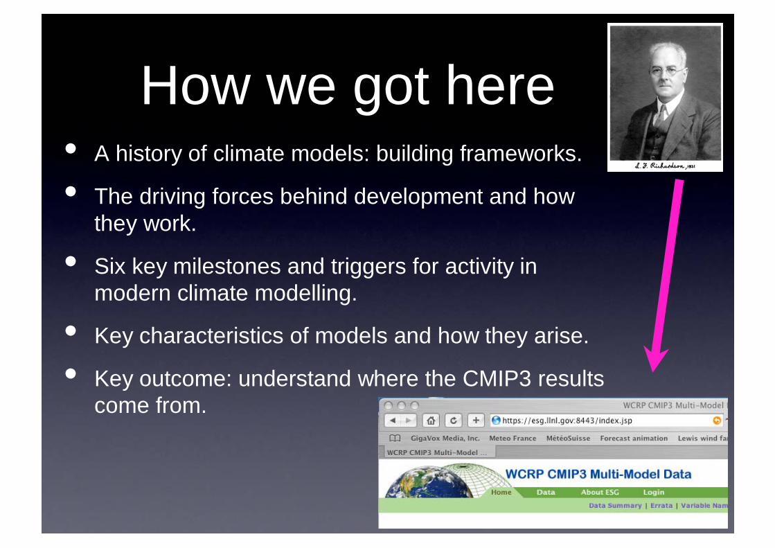
How we got here• A history of climate models: building frameworks.

• The driving forces behind development and how they work.

• Six key milestones and triggers for activity in modern climate modelling.

• Key characteristics of models and how they arise.

• Key outcome: understand where the CMIP3 results come from.

In the beginning• By the 19th century, the pattern of winds on the globe is mapped

and the search for explanations based on our understanding of a heated rotating sphere begins.

• Explanations of climate are little more than story-telling and hand-waving.

• In 1897, Bjerknes constructs the equations that describe a the motion and thermodynamics of a non-homogeneous fluid.

• Bjerknes argues that a physical description of the atmosphere could be used for prediction “Hopefully, the time will also soon come, when a complete statement of atmospheric conditions can be made either daily or on specified dates. At that point, the first condition for scientific weather forecasting will be met.” Published in the Magazine of Meteorology, January 1904(Meteorologische Zeitschrift)

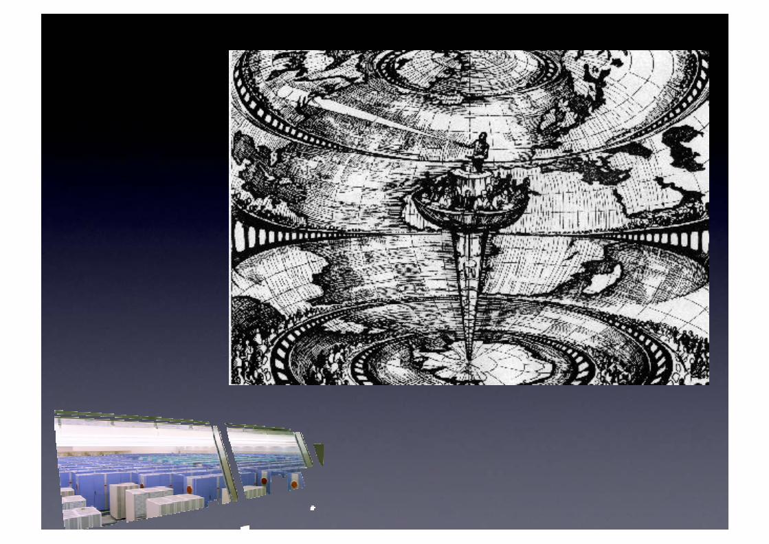
• L.F. Richardson formulates numerical basis for weather forecasts

Richardson developed a scheme for numerical prediction of the atmospheric state. His experiment did not produced a realistic result and he concluded that “The scheme is complicated because the atmosphere itself is complicated.

He envisages a

‘forecast factory’

After 6 weeks of pencil work, he wonders if one in the dim future it will be possible to advance the calculations faster than the weather advances.

History• History is, more or less, bunk. — Henry Ford

• A chronological record of significant events—Webster’s Dictionary

• History is indeed little more than the register of the crimes, follies, and misfortunes of mankind —Edward Gibbon

• There is properly no history; only biography —Ralph Waldo Emerson

If you would understand anything, observe its beginning and its development.— AristotleHistory is the distillation of rumour.

— Thomas Carlyle

For my part, I consider that it will be found much better by all parties to leave the past to history, especially as I propose to write that history myself.Winston Churchill

History

• History, real solemn history, I cannot be interested in.... I read it a little as a duty; but it tells me nothing that does not either vex or weary me. The quarrels of popes and kings, with wars and pestilences in every page; the men all so good for nothing, and hardly any women at all - it is very tiresome. — Jane Austen (from Northanger Abbey)

Today we have coupled models

incorporating many aspects of

the climate system.

How did we get here and how do we use the tools available to go

further?

Climate Model Pyramid

• A simple description of climate models is the climate modelling pyramid.

• Simple models are at the base and more complex models at the top.

• Higher means more complex, but not necessarily ‘better’.

GFDL

NCAR

IPCC

GISS

UKMO

‘data’ from Spencer Weart’s AIP page

Factors affecting population development

• Mutation: a sudden change in genotype caused by a small change in the DNA

• Gene flow: genetic material flows from other populations

• Natural selection: some environments favour certain characteristics and these individuals come to dominate the population

• Genetic Drift: changes due to random chance

• Inbreeding & Inbreeding Depression: a restricted pool of genetic material leads to a reduction in vigour due to expression of deleterious recessive alleles.

Between population diversity

• populations diverge for a number of reasons

• natural selection (of parameterisations)

• genetic drift (modellers get smarter and have lucky breaks)

• mutations (e.g. funding cuts and increases)

• gene flow: movement of scientists and information reduces inter-population variation Natural selection

genetic drift

mutation

gene flow

Within population variation

• Variation within a population is controlled (reduced) by

• natural selection (the best individuals dominate)

• genetic drift

• inbreeding (leads to reduced vigour)

• increased by gene flow and mutation (new model versions created)

Natural selection

genetic drift

mutation gene flow

inbreeding

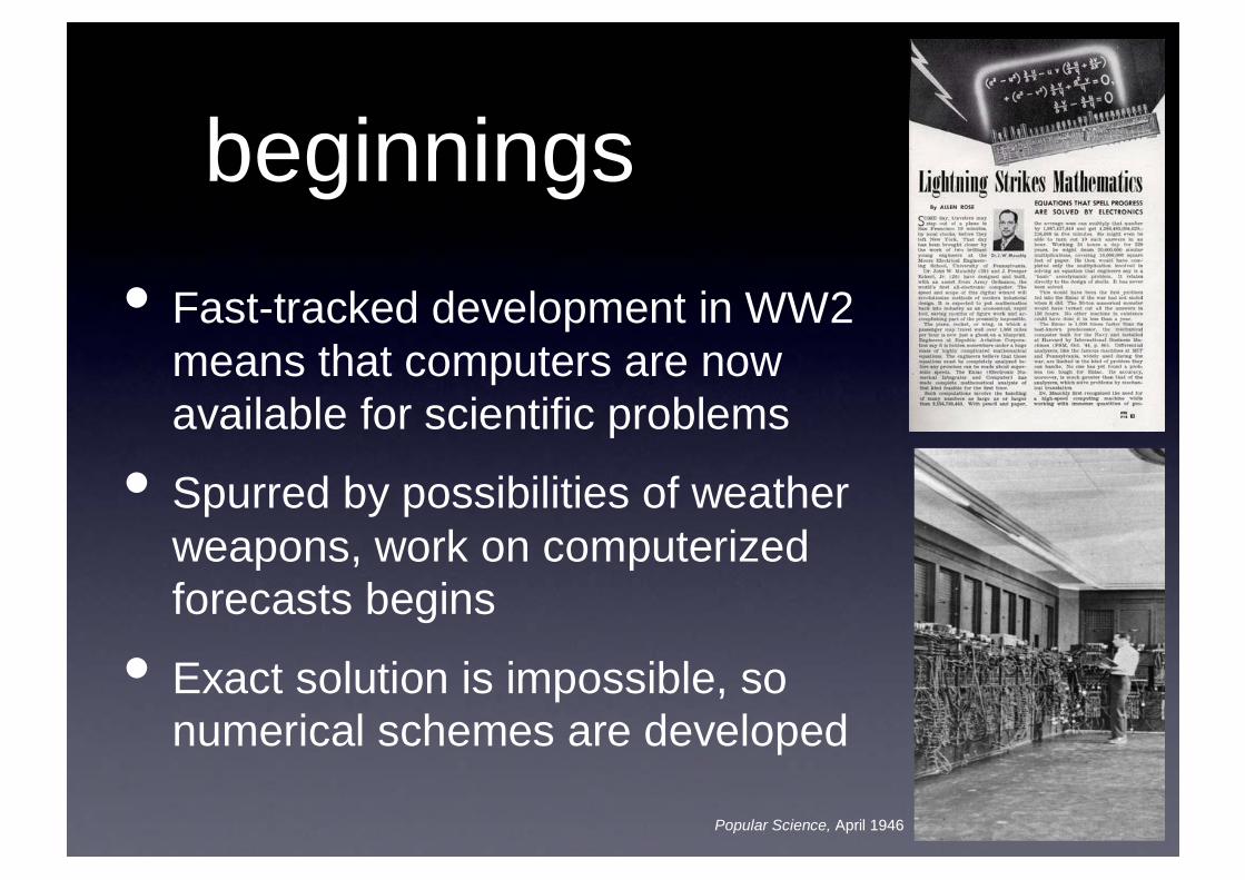
beginnings• Fast-tracked development in WW2

means that computers are now available for scientific problems

• Spurred by possibilities of weather weapons, work on computerized forecasts begins

• Exact solution is impossible, so numerical schemes are developed

Popular Science, April 1946April 1946

In 1952 Bert Bolin concluded that “there is very little hope for the

possibility of deducing a theory for the general

circulation of the atmosphere from the

complete hydrodynamic and thermodynamic

equations.

Already Von Neuman had started working on numerical computations

of the atmosphere

Smagorinsky

Charney

by 1949, results were looking fairly realistic.

“the machine will give a greater scope to the

making and testing of physical hypotheses”

Forties and Fifties

Arakawa, Manabe, Phillips, Wetherald, Mintz,

Milestone1. The Transistor

Early years: the invention of a machine

• Formulation of models

• Direct programming of hardware by a few individuals

• Dealing with new paradigms poses problems (what is status of model output)

• Computers still barely able to do the job required

Early highlights• Von Neuman sees parallels between explosion simulations and

weather predictions and advocates the use of computers

• Jules Charney is invited to head a new meteorology group and by 1950 has a 24 hour forecast that takes 24 hours to produce a 24 hour forecast (700km grid over USA)

• Charney’s success sparks further action. By 1958 Smagorinsky has employed a young Japanese physicist (Manabe) who goes on to build one of the longest lasting GCM programmes.

• Manabe studies all aspects of the climate system and by 1965, the lab has a nine level model of the global atmosphere (no geography)

• Meanwhile at UCLA, a young Arakawa has been recruited and by 1964 has a 2 layer, global model with geography, moutains, oceans and ice (representations anyway)

Milestone 2: FORTRAN

1960s and FORTRAN• High level languages and ‘programmers’

are invented. Scientists can now focus on science.

• Modelling at this point is a secret society. Programming is a complex task, heavily machine dependent. Higher level languages are primitive compared to today and storage capacity is minimal.

• At this point, models begin to emerge around the world as computers improve and knowledge spreads. Gene flow increases but mutations and genetic drift dominate.

1960s• Decent simulations of climate (e.g.

Smagorinksy, 1963; Leith, 1965)

• Development of ocean model (Bryan, 1969; Manabe & Bryan, 1969)

• 1D RC simulations (Manabe & Wetherald, 1967)

• Role of the surface hydrology (Manabe, 1969)

• Energy Balance Models (Budyko 1969; Sellers, 1969)

• Credibility established and conceptual aspects being explored

60s• Basic building blocks are

constructed and modellers begin to expand their horizons

• Implementation is ‘basic’ at best

• Computers are getting better but still a rare and expensive resource

• ...enter Seymour Cray

Milestone 3: Supercomputer

1970s• Computers keep getting bigger, storage

improves, understanding improves

• Modellers start to catalogue their tools

• Recognition of a lack of knowledge about the real atmosphere spawns GARP and FGGE (1979)

• Modelling begins to develop different schools of thought that continue to this day

Classifying modellers• Seers & formalists emerge as genres

• Seers: Model’s simulated climate has many characteristics of the real climate the important features are included (ocean, atmosphere, surface hydrology)

• Formalists pursue detail

• In the 70s, a heirarchy begins to emerge (e.g. Schneider and Dickinson) and modelling continues to develop.

At this time, we see the

emergence of ‘model

experiments’and a framework

for analysis of these

experiments

70s classics• Manabe & Wetherald 1975; Effects of CO2

doubling

• Chervin et al 1976; On determining statistical significance

• Bourke et al., 1977 Modelling using spectral methods

• Schneider and Dickinson, 1974, Review of Climate Modelling

• GARP 1975

Milestone 4: Sub-second response

1980s• The arrival of sub-second

response and interactive desktop computing

• The Economic Value of Rapid Response TimeNovember, 1982 W. J. Doherty, A. J. Thadani, “When a computer and its users interact at a pace that ensures that neither has to wait on the other, productivity soars, the cost of the work done on the computer tumbles, employees get more satisfaction from their work, and its quality tends to improve”.

System response timeTr

ansa

ctio

ns p

er h

our (

prod

uctiv

ity)

The rise of the formalists

• You can never have too much detail

• push to higher resolution

• push to longer simulations

• push for more processes (soil layers, stomates, crops, trees, rivers, sea ice etc.)

• the model is an end in itself

The formalists begin to dominate as the balance of external forces

changes

80s classics

• Semtner & Chervin, 1988

• Sellers et al., 1986 (SiB)

• Henderson-Sellers &Wilson 1983

• Washington et al., 1980

5. WWW

1990s: Intercomparisons and

Assessments• New communications spurs better

documentation and sharing of data

• New generation of code sharing

• Model intercomparison projects abound

• IPCC begins to influence community

90s classics

• Cess et al., 1989 (FANGIO)

• Cess et al., 1991 (Snow-Climate Feedback analysis and intercomparison)

• Gates, 1992, AMIP

• IPCC Assessment reports begin to frame progress

6. Giant Magneto-resistance

Hadley Centre

• Greene, M.T., 2006, Looking for a General for some Modern Major Models, Endeavour, 30, 55–59.

Isolated model future

Rich modelers

Under-resourced

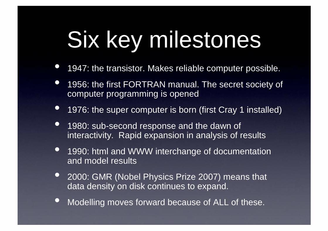
Six key milestones• 1947: the transistor. Makes reliable computer possible.

• 1956: the first FORTRAN manual. The secret society of computer programming is opened

• 1976: the super computer is born (first Cray 1 installed)

• 1980: sub-second response and the dawn of interactivity. Rapid expansion in analysis of results

• 1990: html and WWW interchange of documentation and model results

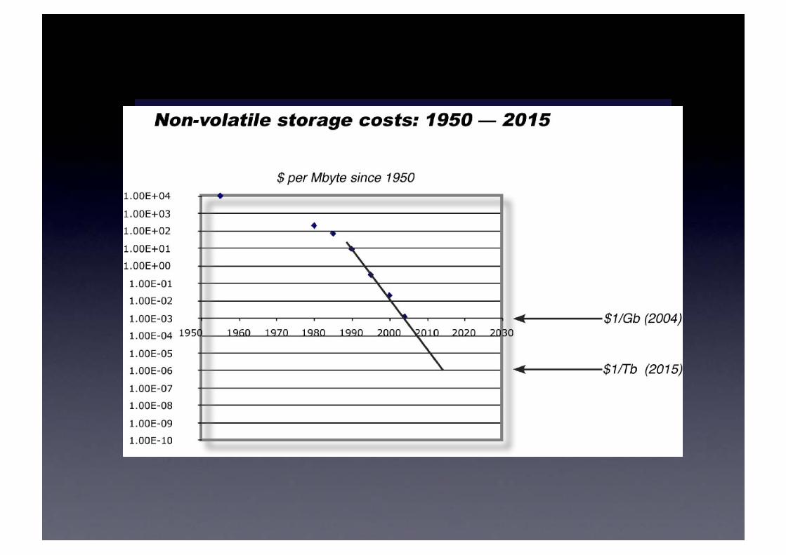
• 2000: GMR (Nobel Physics Prize 2007) means that data density on disk continues to expand.

• Modelling moves forward because of ALL of these.

END OF PRESENTATION