13-1

Copyright © 2005 by The McGraw-Hill Companies, Inc. All rights reserved. McGraw-Hill/Irwin

13

Performance Evaluation and Risk Management

13-3

It is Not the Return On My Investment ...

“It is not the return on my investmentthat I am concerned about.

It is the return of my investment!”

– Will Rogers

13-4

However,

“We’ll GUARANTEE you a 25% return of your investment!”

– Tom and Ray Magliozzi

13-5

Performance Evaluation and Risk Management

• Our goals in this chapter are to learn methods of – Evaluating risk-adjusted investment performance, and – Assessing and managing the risks involved with specific

investment strategies

13-6

Performance Evaluation

• Can anyone consistently earn an “excess” return, thereby “beating” the market?

• Performance evaluation is a term for assessing how well a money manager achieves a balance between high returns and acceptable risks.

13-7

Performance Evaluation Measures

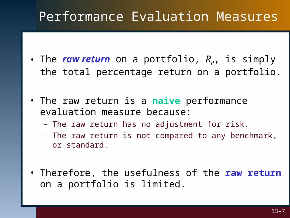
• The raw return on a portfolio, RP, is simply the total percentage return on a portfolio.

• The raw return is a naive performance evaluation measure because:– The raw return has no adjustment for risk.– The raw return is not compared to any benchmark, or standard.

• Therefore, the usefulness of the raw return on a portfolio is limited.

13-8

Performance Evaluation Measures

The Sharpe Ratio

• The Sharpe ratio is a reward-to-risk ratio that focuses on total risk.

• It is computed as a portfolio’s risk premium divided by the standard deviation for the portfolio’s return.

p

fp

σ

RRratio Sharpe

13-9

Performance Evaluation Measures

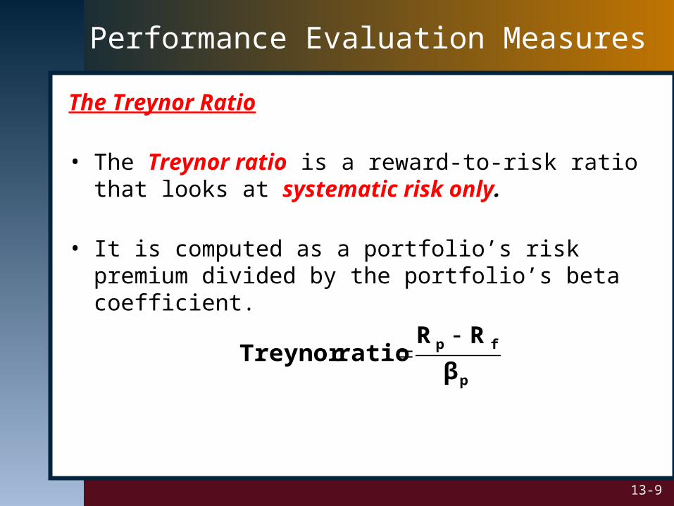
The Treynor Ratio

• The Treynor ratio is a reward-to-risk ratio that looks at systematic risk only.

• It is computed as a portfolio’s risk premium divided by the portfolio’s beta coefficient.

p

fp

β

RRratio Treynor

13-10

Performance Evaluation Measures

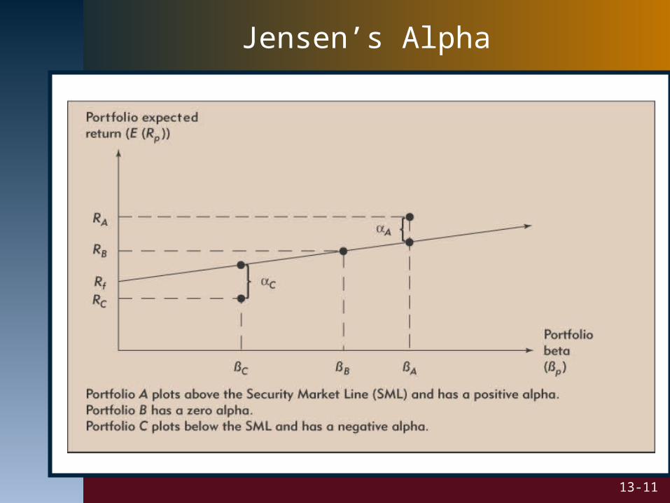
Jensen’s Alpha

• Jensen’s alpha is the excess return above or below the security market line. It can be interpreted as a measure of how much the portfolio “beat the market.”

• It is computed as the raw portfolio return less the expected portfolio return as predicted by the CAPM.

Actual return

CAPM Risk-Adjusted ‘Predicted’ Return“Extra” Return

RREβ R Rα fMpfpp

13-11

Jensen’s Alpha

13-12

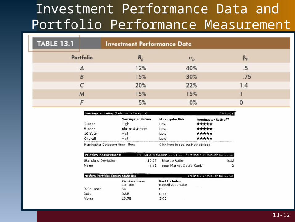
Investment Performance Data and Portfolio Performance Measurement

13-13

Comparing Performance Measures, I.

• Because the performance rankings can be substantially different, which performance measure should we use?

Sharpe ratio:

• Appropriate for the evaluation of an entire portfolio.

• Penalizes a portfolio for being undiversified, because in general, total risk systematic risk only for relatively well-diversified portfolios.

13-14

Comparing Performance Measures, II.

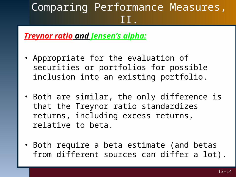
Treynor ratio and Jensen’s alpha:

• Appropriate for the evaluation of securities or portfolios for possible inclusion into an existing portfolio.

• Both are similar, the only difference is that the Treynor ratio standardizes returns, including excess returns, relative to beta.

• Both require a beta estimate (and betas from different sources can differ a lot).

13-15

Sharpe-Optimal Portfolios, I.

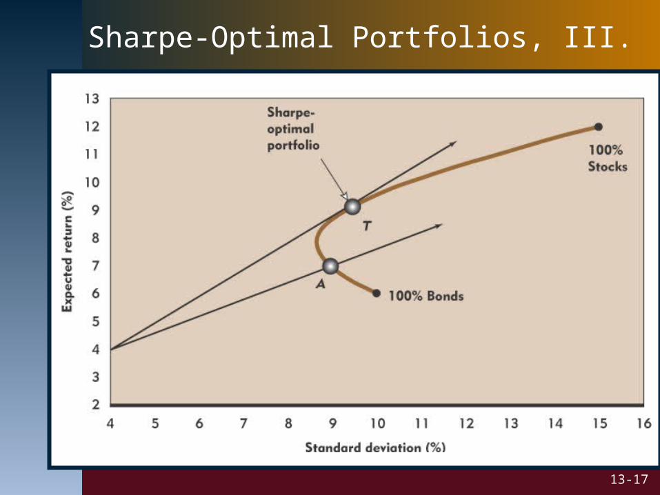
• Allocating funds to achieve the highest possible Sharpe ratio is said to be Sharpe-optimal.

• To find the Sharpe-optimal portfolio, first look at the plot of the possible risk-return possibilities, i.e., the investment opportunity set.

ExpectedReturn

Standard deviation

××

××

×

×

××

×

×

×× ×

×

×

×

13-16

ExpectedReturn

Standard deviation

× A

Rf

A

fA

σ

RREslope

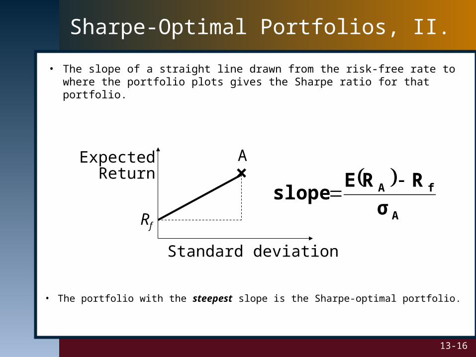
Sharpe-Optimal Portfolios, II.

• The slope of a straight line drawn from the risk-free rate to where the portfolio plots gives the Sharpe ratio for that portfolio.

• The portfolio with the steepest slope is the Sharpe-optimal portfolio.

13-17

Sharpe-Optimal Portfolios, III.

13-18

Example: Solving for a Sharpe-Optimal Portfolio

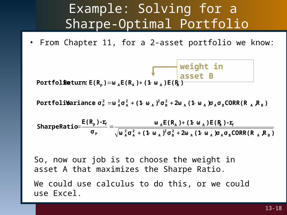
• From Chapter 11, for a 2-asset portfolio we know:

So, now our job is to choose the weight in asset A that maximizes the Sharpe Ratio.

We could use calculus to do this, or we could use Excel.

)R,CORR(Rσ)σω(12ωσ)ω(1σω

r -))E(Rω(1)E(Rω

σ

r-)E(RRatio Sharpe

)R,CORR(Rσ)σω(12ωσ)ω(1σωσ : VariancePortfolio

))E(Rω(1)E(Rω)E(R :Return Portfolio

BABAAA2B

2A

2A

2A

fBAAA

P

fp

BABAAA2B

2A

2A

2A

2P

BAAAp

weight in asset B

13-19

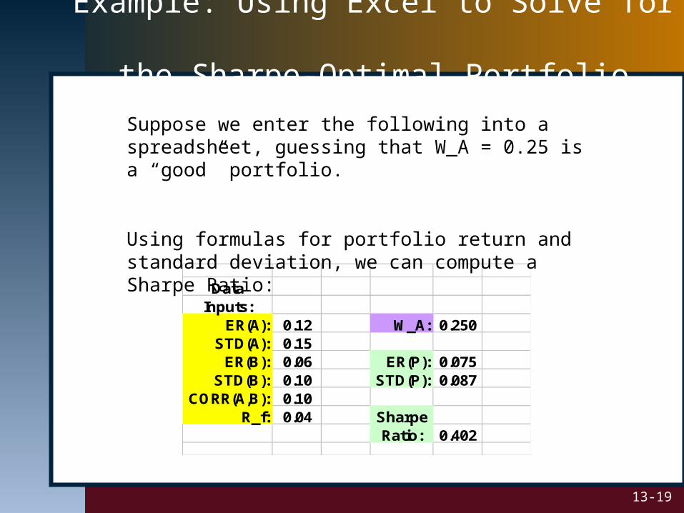
Example: Using Excel to Solve for the Sharpe-Optimal Portfolio

DataInputs:

ER(A): 0.12 W_A: 0.250STD(A): 0.15

ER(B): 0.06 ER(P): 0.075STD(B): 0.10 STD(P): 0.087

CORR(A,B): 0.10R_f: 0.04 Sharpe

Ratio: 0.402

Suppose we enter the following into a spreadsheet, guessing that W_A = 0.25 is a “good” portfolio.

Using formulas for portfolio return and standard deviation, we can compute a Sharpe Ratio:

13-20

Example: Using Excel to Solve for the Sharpe-Optimal Portfolio, Cont.

• Now, we let Excel solve for the weight in portfolio A that maximizes the Sharpe Ratio.

• We use the Solver, found under Tools.

Data ChangerInputs: Cell:

ER(A): 0.12 W_A: 0.700STD(A): 0.15

ER(B): 0.06 ER(P): 0.102STD(B): 0.10 STD(P): 0.112

CORR(A,B): 0.10R_f: 0.04 Sharpe

Ratio: 0.553

Solving for the Optimal Sharpe Ratio

Given the data inputs below, we can use theSOLVER function to find the Maximum Sharpe Ratio:

Target Cell Well, the guess of 0.25 was a tad low….

13-21

Investment Risk Management

• Investment risk management concerns a money manager’s control over investment risks, usually with respect to potential short-run losses.

• We will focus on what is known as the Value-at-Risk (VaR) approach.

13-22

Value-at-Risk (VaR)

• Value-at-Risk (VaR) is a technique of assessing risk by stating the probability of a loss that a portfolio may experience within a fixed time horizon.

• If the returns on an investment follow a normal distribution, we can state the probability that a portfolio’s return will be within a certain range, if we have the mean and standard deviation of the portfolio’s return.

13-23

Example: VaR Calculation

• Suppose you own an S&P 500 index fund.

• What is the probability of a return of -7% or worse in a particular year?

• That is, one year from now, what is the probability that your portfolio value is down by 7 percent (or more)?

13-24

Example: VaR Calculation, II.

• First, the historic average return on the S&P index is about 13%, with a standard deviation of about 20%.– A return of -7 percent is exactly one standard deviations below

the average, or mean (i.e., 13 – 20 = -7).– We know the odds of being within one standard deviation of the

mean are about 2/3, or 0.67.

• In this example, being within one standard deviation of the mean is another way of saying that:

Prob(13 – 20 RS&P500 13 + 20) 0.67

or Prob (–7 RS&P500 33) 0.67

13-25

Example: VaR Calculation, III.

• That is, the probability of having an S&P 500 return between -7% and 33% is 0.67.

• So, the return will be outside this range one-third of the time.

• When the return is outside this range, half the time it will be above the range, and half the time below the range.

• Therefore, we can say: Prob (RS&P500 –7) 1/6 or 0.17

13-26

Example: A Multiple Year VaR, I.

• Once again, you own an S&P 500 index fund.

• Now, you want to know the probability of a loss of 30% or more over the next two years.

• As you know, when calculating VaR, you use the mean and the standard deviation.

• To make life easy on ourselves, let’s use the one year mean (13%) and standard deviation (20%) from the previous example.

13-27

Example: A Multiple Year VaR, II.

• Calculating the two-year average return is easy, because means are additive. That is, the two-year average return is:

13 + 13 = 26%

• Standard deviations, however, are not additive.

• Fortunately, variances are additive, and we know that the variance is the squared standard deviation.

• The one-year variance is 20 x 20 = 400. The two-year variance is:

400 + 400 = 800.

• Therefore, the 2-year standard deviation is the square root of 800, or about 28.28%.

13-28

Example: A Multiple Year VaR, III.

• The probability of being within two standard deviations is about 0.95.

• Armed with our two-year mean and two-year standard deviation, we can make the probability statement:

Prob(26 – 228 RS&P500 26 + 228) .95

or

Prob (–30 RS&P500 82) .95

• The return will be outside this range 5 percent of the time. When the return is outside this range, half the time it will be above the range, and half the time below the range.

• So, Prob (RS&P500 –30) 2.5%.

13-29

Computing Other VaRs.

• In general, for a portfolio, if T is the number of years,

5%Tσ1.645TRERProb

2.5%Tσ1.96TRERProb

1%Tσ2.326TRERProb

ppTp,

ppTp,

ppTp,

TRERE pTp, Tσσ pTp,

Using the procedure from before, we make make probability statements. Three very useful one are:

13-30

Useful Websites

• www.stanford.edu/~wfsharpe (visit Professor Sharpe’s homepage)

• www.morningstar.com (Comprehensive source of investment information)

• www.gloriamundi.org (learn all about Value-at-Risk)

• www.garp.org (The Global Association of Risk Professionals)

• www.riskmetrics.com (Check out risk grades)

13-31

Chapter Review

• Performance Evaluation– Performance Evaluation Measures

• The Sharpe Ratio• The Treynor Ratio• Jensen’s Alpha

• Comparing Performance Measures– Sharpe-Optimal Portfolios

• Investment Risk Management– Value-at-Risk (VaR)

• More on Computing Value-at-Risk