Determination of the blocking temperature of magnetic nanoparticles:The good, the bad and the ugly

P. Mendoza Zelis,1, 2, a) I.J. Bruvera,1, b) M.Pilar Calatayud,3, 4 G.F. Goya,3, 4 and F.H. Sanchez11)IFLP-CCT- La Plata-CONICET and Departamento de Fısica, Facultad de Ciencias Exactas, C. C. 67,Universidad Nacional de La Plata, 1900 La Plata, Argentina2)Departamento de Ciencias Basicas, Facultad de Ingenierıa, Universidad Nacional de La Plata, 1900 La Plata,Argentina3)Aragon Institute of Nanoscience (INA), University of Zaragoza, 50018, Spain4)Condensed Matter Physics Department, Science Faculty, University of Zaragoza, 50009,Spain

In a magnetization vs. temperature (M vs. T) experiment, the blocking region of a magnetic nanoparticle(MNP) assembly is the interval of T values were the system begins to respond to an applied magnetic fieldH when heating the sample from the lower reachable temperature. The location of this region is determinedby the anisotropy energy barrier depending on the applied field H, the volume V, the magnetic anisotropyconstant K of the MNPs and the observing time of the technique. In the general case of a polysized sample,a representative blocking temperature value TB can be estimated from ZFC-FC experiments as a way todetermine the effective anisotropy constant.

In this work, a numerical solved Stoner-Wolfharth two level model with thermal agitation is used to sim-ulate ZFC-FC curves of monosized and polysized samples and to determine the best method for obtaining arepresentative TB value of polysized samples. The results corroborate a technique based on the T derivativeof the difference between ZFC and FC curves proposed by Micha et al (the good) and demonstrate its relationwith two alternative methods: the ZFC maximum (the bad) and inflection point (the ugly). The derivativemethod is then applied to experimental data, obtaining the TB distribution of a polysized Fe3O4 MNP samplesuspended in hexane with an excellent agreement with TEM characterization.

I. INTRODUCTION

Magnetic nanoparticles (MNPs) are been extensivelystudied due to their multiple applications in technology1

and biomedicine2,3. Particles with sizes in the range[5, 100]nm4 present a magnetic behaviour determined byits volume, shape and composition, matrix viscosity andtemperature, among other factors. In the simplest (how-ever very useful) model, the MNPs of volume V and satu-ration magnetization Ms are considered as almost spher-ical ellipsoids with a permanent moment m = MsV anda preferential magnetization axis (easy axis) in which theanisotropy energy EK = KV sin2[δ] is minimum, beingK the effective anisotropy density constant and δ the an-gle between m and the easy axis. If the MNPs are fixedin the matrix and separated one from each other by a dis-tance d > 3V 1/3, dipolar interactions can be neglected5

and the energy of the system can be expressed as thesum of the anisotropy energy and the Zeeman energyEH = −mH cos[θ]:

E = EK + EH , (1)

with θ the angle between m and H (fig. 1). This config-uration is usually called Stoner-Wolfharth system sincethe publication of a work6 in which the authors perform

a)Electronic mail: pmendoza@fisica.unlp.edu.arb)Electronic mail: bruvera@fisica.unlp.edu.ar

a numerical calculation of the M vs. H curves of orderedsystems with different orientations i.e. systems of identi-cal MNPs with a single value of φ, and the M vs.H curveof a disordered system i.e. with a uniform distribution ofφ values. Since no thermal agitation was considered byStoner and Wolfharth, their calculations were made justfinding the positions θi of the minima of equation 1 foreach value of H.

FIG. 1. MNP model. The energy is determined by the angle δbetween the magnetization M and the field H, and the angleθ between M and the easy axis K. For calculation simplicitythe angle φ = θ + δ between K and H is used.

In order to calculate the temperature dependence ofthe magnetic response for MNPs systems, it is neces-sary to consider the effect of thermal fluctuations that

arX

iv:1

508.

0441

3v1

[co

nd-m

at.m

es-h

all]

18

Aug

201

5

2

allow transitions between stable configurations. Doingso, it is possible to simulate M vs. T experiments as theextensively performed Zero Field Cooling-Field Cooling(ZFC-FC) routine. In this kind of experiments, a sampleis cooled from a temperature where all particles show su-perparamagnetic behaviour to the lowest reachable tem-perature (usually around 3K), then, a small constantfield usually lower than 8kA/m is applied, and the sam-ple is heated to a temperature high enough to observe aninitial growth and subsequent decrease in magnetization,i.e. were the sample show again superparamagnetic be-haviour .The sample is then cooled again to the lowesttemperature with the constant field still applied.

In the ideal case of a monosized, non interacting MNPssample; a narrow temperature region should exist inwhich the system performs a transition between irre-versible and reversible regimes. When heating withapplied field, the thermal energy kT is initially muchsmaller than the anisotropy barrier KV so the magne-tization remains null. Due to the exponential depen-dence of the Neel relaxation time with temperature7,when kT ∼ KV , the magnetization grows rapidly untilits thermodynamic equilibrium value, defining the afore-mentioned transition region. The Blocking TemperatureTB can be considered as the inflection point of this grow-ing and its experimental determination is an importantgoal of the MNPs characterization.

Real samples always present a size dispersion, usuallyreasonably well described by a log-normal distribution.Different particle size implies different anisotropy bar-rier KV and therefore a different TB for each size frac-tion, so, in real ZFC-FC experiments, the blocking re-gion is wide and the representative TB value is not welldefined. There are several different criteria used to de-fine a representative TB from ZFC-FC data of polysizedsamples. Some authors maintain the inflexion point (IP)criterion8 while others report the maximum ZFC mag-netization temperature (MAX)910, being all this criteriastill in discussion11. In an alternative approach, Michaet al.12 propose a method in which the TB distribution isobtained from the T derivative of the difference betweenZFC and FC curves. An approximated theoretical jus-tification for this method was presented by Mamiya etal13.

In this work, a SW model with thermal agitation isapplied to obtain the temporal dependence of the mag-netization M(t) for an ordered system of identical MNPsin a similar way to previous works of Lu14, Usov15

and Carrey16. Temperature dependence dM(T )/dT isthen obtained in order to numerically simulate the ZFC-FC curves. In contrast to the method implemented byUsov17 where a stair-step approximation for the time evo-lution of the temperature was used, we consider a con-tinuous time evolution. Finally, an ordered polysize sys-tem response is simulated by linear combination of themonosize curves weighted by a discrete log-normal dis-tribution.

The validity of the method proposed by Micha et al

was verified by comparing the T derivative of this ZFC-FC curve with the TB distribution obtained from theinflection points of each volume of the distribution. Theresultant mean blocking temperature value < TB > isthen compared, for several volume distributions, with thecommonly used criteria for a representative TB : the in-flection point temperature IP and the maximum MAX ofthe ZFC curve.

Additionally, Micha’s method is tested with experi-mental data of a magnetite MNPs frozen ferrofluid sus-pended in hexane comparing the obtained TB distribu-tion with the one calculated from the TEM size informa-tion. In order to obtain an ordered system, the ferrofluidwas frozen while a large constant was field applied.

II. MODEL

A SW-like model with thermal agitation and zerowidth energy minima approximation was developed inorder to obtain ZFC-FC curves of fixed MNPs with sizedispersion. Only the simplest case of an ordered systemwas considered, with all the MNPs oriented (easy axisorientation) in the direction of the field. This situationcan be achieved experimentally by freezing a ferrofluidsample under a sufficiently strong applied field (∼ 7T ).

A. Magnetization vs. time equation

For a system of identical, fixed, non interacting MNPsof volume V , anisotropy constant K and saturation mag-netization Ms, with their anisotropy axes parallel to anexternal field H, the energy can be expressed as the sumof the anisotropy energy Ek and the Zeeman energy Eh

6:

E = Ek + Eh = KV Sin(θ)2 − µ0MsV Cos(θ)

= KV

(Sin(θ)2 − 2hCos(θ)

),

(2)

being h = H/Hk and Hk = µ0Ms/2K.In the range θ = [0, 2π], this energy landscape presents

two minima, of E(0) = −2KVh and E(π) = 2KVh and a

maximum of E(arccos(−h)) = KV

(1 + h2

)(fig. 2).

The frequency of thermal inversions between minima iand j is the inverse of the Neel relaxation time1819,:

fij = f0eDij/(kT ) (3)

with f0 the “intrinsic frequency”, times the Boltzman“success probability” depending on the ratio betweenthermal energy kT and barrier height Dij . The barrierbetween minima is symmetric for h = 0 with Ddu =Dud = KV (naming u and d to θ = 0 and θ = π direc-tions respectively) and smaller for inversion to the field

3

Π

2Π

3 Π

2Π 2 Π

-2

-1

0

1

2

Θ

E�K

V

t

FIG. 2. Energy landscapes as a function of theta for a fixedMNP under a magnetic field at θ = 0. Each color stands for adifferent value of the reduced field factor 2h. Blue: 2h = 0.1,purple: 2h = 0.5, gold: 2h = 2.

direction otherwise:

∆ud = E(arccos(−h))− E(π) = KV

(1 + h

)2

∆du = E(arccos(−h))− E(0) = KV

(1− h

)2(4)

It is a good approximation to consider the same f0value for both frequencies20.

Sample magnetization M in the direction of the ap-plied field can be expressed in terms of saturation magne-tization Ms and the number of particles per unit volumemagnetized in each direction Nu and Nd:

M =

(Nu −Nd

)Ms/N = Ms

(2Nu/N − 1

), (5)

with N the total number of particles per unit volume. Sothe time derivative of the magnetization can be writtenin terms of the population variation which is equal to theactual population times the inversion probability to eachdirection

dM

dt= 2

Ms

N

dNu

dt. (6)

dNu

dt= −dNd

dt= fd→uNd − fu→dNu. (7)

so the time derivative of the relative magnetization m isdetermined by the transcendental equation

dm

dt= 2f0e

−C(1+h2

){sinh(2C h)−m cosh(2C h)}. (8)

where C = KV/kT .

FIG. 3. Simulation result for an ordered assembly of MNPs.The system is first cooled with zero field applied from a hightemperature where all particles show superparamagnetic be-haviour (ZFC, no showed), then, the field is turned on and thesystem is heated beyond the blocking region (ZFCW). Main-taining the applied field, the system is cooled (FC). The finalheating can be performed with (FCW) or without appliedfield (TRM).

B. Magnetization vs. Temperature equation: ZFC-FCsimulation

Temperature dependence of the magnetization can beobtained from 8 via the equation

dm

dT=dm

dt

dt

dT. (9)

For a linear temperature variation T (t) = Bt+T0, themagnetization derivative is

dm

dT=

1

B

dm

dt=

2f0Be−C

(1+h2

){sinh(2C h)−m cosh(2C h)}

(10)Solving this equation by numerical methods it is pos-

sible to simulate a ZFC-FC experiment for a monosizesample. A Matlab script based on the ODE15s21 func-tion was developed. An example of the result for a mono-size assembly of ordered MNPs is shown in figure 3. Linecolours stand for different parts of the routine.

During the warming after zero field cooling (ZFCWfor this chapter, usually called just ZFC), the exponen-tial dependence of the inversion frequency with tempera-ture in equation 3 determines a narrow “blocking region”wherein the MNPs, which were “blocked” at low temper-ature begin to respond to the field. Magnetization growswith temperature since the applied field has decreasedthe energy barrier for θ = π to θ = 0 inversion. Themagnetization increasing reverts when thermal energy is

4

FIG. 4. Comparison between ZFC-FC simulations for small(σ = 10−8) and large (σ = 0.5) dispersion systems.

much higher than the barrier, so the difference betweeninversion frequencies in each direction tends to disappear.The blocking temperature TB of the system is then de-fined as the inflection point of the magnetization growingwhen heating.

When the system is cooled again (FC), magnetiza-tion grows monotonically while the barrier height differ-ence between inversions becomes increasingly significantagainst thermal energy. This growth stops when thermalenergy becomes too low for inversions to occur withinthe experimental window time. If the system is thenheated maintaining the applied field (FCW), magnetiza-tion values are the same than FC except for the blockingregion where there is a small increase due to the assem-bly getting closer to the equilibrium state. If the finalwarming is done with no applied field (Thermal Rema-nent Magnetism, TRM), magnetization drops to zero inthe blocking region when thermal energy is enough forthe wells populations to equilibrate.

The magnetization values Mp for a polysized sampleare obtained by linear addition of the MV i values foreach contemplated size Vi, weighted by the correspondingvolume and log-normal distribution LnN(Vi) value:

Mp(T ) =

∑Ni=1MV i(T )ViLnN(V )∑N

i=1 ViLnN(V ), (11)

The ViLnN(Vi) product stands for the relative volumedistribution.

Figure 4 shows the comparison between ZFC-FC sim-ulations for samples with different size dispersion ex-pressed as the scale parameter σ of the log-normal num-ber distribution. A much wider transition region can beseen for the bigger dispersion so the different aforemen-tioned criteria would define very separated values for arepresentative TB .

FIG. 5. Scheme of the method verification. Monosize ZFC-FC curves are simulated from the dM(T)/dT equations of themodel. In one path, TB for every particle size is calculatedas the IP of the monosize ZFC curve. In the other path,a polysize ZFC-FC curve is simulated by linear addition ofthe monosize values. Then the T derivative of the differenceZFC-FC is calculated.

III. BLOCKING TEMPERATURE DETERMINATION

A. Micha’s method verification

In order to verify Micha’s method, several polysizeZFC-FC experiments were simulated using differents pa-rameter sets varying σ and the mean radius. For eachone of the used sets, the T derivative of the ZFC-FC dif-ference was calculated. Then, the TB distribution wasobtained from the monosize curves that were added toconstruct the polyzise simulation in equation 11: a ZFCcurve was calculated for each class of the size distributionso each TB class comes from a volume class, maintain-ing the same relative height. Also IP and MAX valuesof the polysize ZFC curve were calculated and comparedwith the mean value < TB > of the distribution in eachsimulation (fig. 5).

In all cases, the TB distribution and the ZFC-FCderivative are identical. Figure 6 shows the results for thesimulation with 4.5 nm mean radius, σ = 0.5, 16kJ/m3

anisotropy constant and a 4K/min heating rate.Also, for a set of ZFC-FC curves calculated with the

same mean volume, saturation magnetization, heatingrate and anisotropy constant, by increasing scale param-eter σ, < TB > stays constant while the polysize curve IPshifts to smaller temperatures and MAX shifts in oppo-site direction. Figure 7 shows the results for 4.5nm meanradius, 16kJ/m3 anisotropy constant, 4K/min heatingrate and σ = [0.1, 0.6].

This behaviour is the same in the hole studied sizerange. By normalizing IP values by the TB mean, allpoints fall in the same curve as shown in figure 8 whilethe variation for MAX is small.

Varying the heating rate and K does not affect therelation IP/< TB >. Meanwhile, the MAX/< TB >ratio changes strongly in the range [0.04; 400]K/min andnoticeably in the range [1; 10]K/min and also dependson the K value. Figure 9 shows the results of varying

5

FIG. 6. Comparison between the TB distribution obtaineddirectly from the size distribution used in the simulation andthe derivative d(ZFC-FC)/dT of the simulated curves.

FIG. 7. Values of TB mean, MAX and IP of the simulatedcurves as a function of the scale parameter σ for 4.5nm meanradius, 16kJ/m3 anisotropy constant and 4K/min heatingrate.

the heating rate for Rm = 10nm, K = 16kJ/m3 andMs = 281kA/m.

Figure 10 shows a parabolic fit over the IP/ < TB >values obtained for all the simulations. The curve isuniversal with small fluctuations due to numeric reso-lution. The obtained polynomial with fitting errors is

IP<TB> (σ) = 1.00(2)− 0.21(2)σ − 0.79(2)σ2.

B. Experimental application

The Micha’s analysis was conducted on ZFC-FC mea-surements of a FF of magnetite MNPs suspended in hex-ane with a concentration of 12(1)g/L. TEM images were

FIG. 8. Values of MAX (circles) and IP (squares) of thesimulated curves divided by TB mean for different MNP radii.The behavior is the same for all sizes.

FIG. 9. MAX (circles) and IP (squares) relative to < TB >for 10nm NPM mean radius at different temperature rates.

taken in order to determine the size distribution of theparticles (fig 11). A narrow log-normal number diame-ter distribution (LnN(x)) was obtained with a 9.54nmmean and a 1.73nm standard deviation. The relativeTEM volume distribution was obtained from this resultsand fitted with a xLnN(x) function obtaining a scaleparameter σ = 0.55(2).

The ZFC-FC routine was carried with a 2.4K/min rateand a 8kA/m field on an encapsulated FF sample frozenunder a 7T field in order to obtain an ordered systemwith all the MNP easy axes oriented parallel to the field.The ZFC-FC derivative was calculated and fitted with axLnN(x) distribution using the TEM σ as a fixed pa-rameter with a very good correspondence (figure 12).

6

FIG. 10. Parabolic fitting of the universal curve IP/< TB >.

FIG. 11. Size distribution from TEM images. Inset: TEMimage example with a magnification showing the crystallinityof the particles.

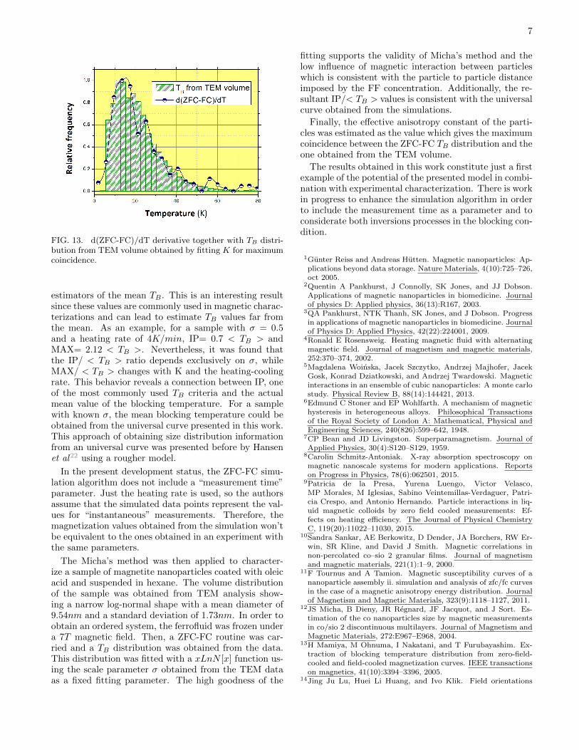
Figure 13 shows the comparison between TB distribu-tion obtained from TEM information and the ZFC-FCderivative curve. The translation from TEM volume toTB was made considering the blocking condition in whichthe inversion time of the MNPs is approximately equalto the measurement time of the magnetization value:

τ(K,V, h, T ) = τ0 exp

(KV

kTB(1− h)2

)≈ τm

⇒ TB =KV (1− h)2

k log(τm/τ0), (12)

where τ0 = 1/f0 is the inverse of the intrinsic inver-sion frequency. For a known volume distribution, thiscomparison can be used to determine the effective K

FIG. 12. Log-normal fit on the d(ZFC-FC)/dT derivative.Inset: ZFC and FC experimental curves.

value as the one that maximizes the coincidence betweenTEM and ZFC-FC distributions. In this case, a value of34(2)kJ/m3 was obtained with a very good correspon-dence between TEM and ZFC-FC data. This calculationimplies some approximations: Ms is considered indepen-dent from the temperature in the region of interest, andthe relaxation time expression used for the blocking con-dition 12 considerate only the inversions in the directionof the field. While the first approximation is very reason-ably, the blocking condition expression is accurate onlyin experiments with high µH/(kT ) ratios, where the re-versal frequency are much smaller for the inversions tothe antiparallel state.

Additionally, the IP/< TB > ratio was calculated ob-taining a value of 0.7(1), compatible with polynomial ex-pression obtained from the simulations.

IV. DISCUSSION AND CONCLUSIONS

The validity of the Micha’s method to determine theTB distribution of non interacting MNPs assembly wasdemonstrated by numerical simulations and experimentaldata analysis.

A Stoner-Wolfarth model with thermal agitation wasdeveloped in order to simulate the ZFC-FC curves ofpolysized MNPs assembles. From this simulation it wasclearly demonstrated that the temperature derivative ofthe ZFC-FC difference is in full coincidence with the TBdistribution of the sample, calculated as the inflectionpoints of each size ZFC curve. Additionally, it cameclear from the results that the maximum (MAX) andthe inflection point (IP) of the polysized ZFC curve areaffected not only by the mean size of the particles, but bythe size dispersion. Thus neither IP or MAX are direct

7

FIG. 13. d(ZFC-FC)/dT derivative together with TB distri-bution from TEM volume obtained by fitting K for maximumcoincidence.

estimators of the mean TB . This is an interesting resultsince these values are commonly used in magnetic charac-terizations and can lead to estimate TB values far fromthe mean. As an example, for a sample with σ = 0.5and a heating rate of 4K/min, IP= 0.7 < TB > andMAX= 2.12 < TB >. Nevertheless, it was found thatthe IP/ < TB > ratio depends exclusively on σ, whileMAX/ < TB > changes with K and the heating-coolingrate. This behavior reveals a connection between IP, oneof the most commonly used TB criteria and the actualmean value of the blocking temperature. For a samplewith known σ, the mean blocking temperature could beobtained from the universal curve presented in this work.This approach of obtaining size distribution informationfrom an universal curve was presented before by Hansenet al22 using a rougher model.

In the present development status, the ZFC-FC simu-lation algorithm does not include a “measurement time”parameter. Just the heating rate is used, so the authorsassume that the simulated data points represent the val-ues for “instantaneous” measurements. Therefore, themagnetization values obtained from the simulation won’tbe equivalent to the ones obtained in an experiment withthe same parameters.

The Micha’s method was then applied to character-ize a sample of magnetite nanoparticles coated with oleicacid and suspended in hexane. The volume distributionof the sample was obtained from TEM analysis show-ing a narrow log-normal shape with a mean diameter of9.54nm and a standard deviation of 1.73nm. In order toobtain an ordered system, the ferrofluid was frozen undera 7T magnetic field. Then, a ZFC-FC routine was car-ried and a TB distribution was obtained from the data.This distribution was fitted with a xLnN [x] function us-ing the scale parameter σ obtained from the TEM dataas a fixed fitting parameter. The high goodness of the

fitting supports the validity of Micha’s method and thelow influence of magnetic interaction between particleswhich is consistent with the particle to particle distanceimposed by the FF concentration. Additionally, the re-sultant IP/< TB > values is consistent with the universalcurve obtained from the simulations.

Finally, the effective anisotropy constant of the parti-cles was estimated as the value which gives the maximumcoincidence between the ZFC-FC TB distribution and theone obtained from the TEM volume.

The results obtained in this work constitute just a firstexample of the potential of the presented model in combi-nation with experimental characterization. There is workin progress to enhance the simulation algorithm in orderto include the measurement time as a parameter and toconsiderate both inversions processes in the blocking con-dition.

1Gunter Reiss and Andreas Hutten. Magnetic nanoparticles: Ap-plications beyond data storage. Nature Materials, 4(10):725–726,oct 2005.

2Quentin A Pankhurst, J Connolly, SK Jones, and JJ Dobson.Applications of magnetic nanoparticles in biomedicine. Journalof physics D: Applied physics, 36(13):R167, 2003.

3QA Pankhurst, NTK Thanh, SK Jones, and J Dobson. Progressin applications of magnetic nanoparticles in biomedicine. Journalof Physics D: Applied Physics, 42(22):224001, 2009.

4Ronald E Rosensweig. Heating magnetic fluid with alternatingmagnetic field. Journal of magnetism and magnetic materials,252:370–374, 2002.

5Magdalena Woinska, Jacek Szczytko, Andrzej Majhofer, JacekGosk, Konrad Dziatkowski, and Andrzej Twardowski. Magneticinteractions in an ensemble of cubic nanoparticles: A monte carlostudy. Physical Review B, 88(14):144421, 2013.

6Edmund C Stoner and EP Wohlfarth. A mechanism of magnetichysteresis in heterogeneous alloys. Philosophical Transactionsof the Royal Society of London A: Mathematical, Physical andEngineering Sciences, 240(826):599–642, 1948.

7CP Bean and JD Livingston. Superparamagnetism. Journal ofApplied Physics, 30(4):S120–S129, 1959.

8Carolin Schmitz-Antoniak. X-ray absorption spectroscopy onmagnetic nanoscale systems for modern applications. Reportson Progress in Physics, 78(6):062501, 2015.

9Patricia de la Presa, Yurena Luengo, Victor Velasco,MP Morales, M Iglesias, Sabino Veintemillas-Verdaguer, Patri-cia Crespo, and Antonio Hernando. Particle interactions in liq-uid magnetic colloids by zero field cooled measurements: Ef-fects on heating efficiency. The Journal of Physical ChemistryC, 119(20):11022–11030, 2015.

10Sandra Sankar, AE Berkowitz, D Dender, JA Borchers, RW Er-win, SR Kline, and David J Smith. Magnetic correlations innon-percolated co–sio 2 granular films. Journal of magnetismand magnetic materials, 221(1):1–9, 2000.

11F Tournus and A Tamion. Magnetic susceptibility curves of ananoparticle assembly ii. simulation and analysis of zfc/fc curvesin the case of a magnetic anisotropy energy distribution. Journalof Magnetism and Magnetic Materials, 323(9):1118–1127, 2011.

12JS Micha, B Dieny, JR Regnard, JF Jacquot, and J Sort. Es-timation of the co nanoparticles size by magnetic measurementsin co/sio 2 discontinuous multilayers. Journal of Magnetism andMagnetic Materials, 272:E967–E968, 2004.

13H Mamiya, M Ohnuma, I Nakatani, and T Furubayashim. Ex-traction of blocking temperature distribution from zero-field-cooled and field-cooled magnetization curves. IEEE transactionson magnetics, 41(10):3394–3396, 2005.

14Jing Ju Lu, Huei Li Huang, and Ivo Klik. Field orientations

8

and sweep rate effects on magnetic switching of stoner–wohlfarthparticles. Journal of applied physics, 76(3):1726–1732, 1994.

15NA Usov and Yu B Grebenshchikov. Hysteresis loops ofan assembly of superparamagnetic nanoparticles with uniaxialanisotropy. Journal of Applied Physics, 106(2):023917, 2009.

16Julian Carrey, Boubker Mehdaoui, and Marc Respaud. Sim-ple models for dynamic hysteresis loop calculations of magneticsingle-domain nanoparticles: Application to magnetic hyperther-mia optimization. Journal of Applied Physics, 109(8):083921,2011.

17NA Usov. Numerical simulation of field-cooled and zero field-cooled processes for assembly of superparamagnetic nanopar-ticles with uniaxial anisotropy. Journal of Applied Physics,109(2):023913, 2011.

18Roger Balian and Dirk Haar. From microphysics to macrophysics:

methods and applications of statistical physics, volume 2.Springer Science & Business Media, 2006.

19L Neel. Influence des fluctuations thermiques a l aimantation desparticules ferromagnetiques. Comptes Rendus de l’Academie desSciences, 228:664–668, 1949.

20Amikam Aharoni. Introduction to the Theory ofFerromagnetism, volume 109. Oxford University Press,2000.

21Lawrence F Shampine and Mark W Reichelt. The matlab odesuite. SIAM journal on scientific computing, 18(1):1–22, 1997.

22Mikkel Fougt Hansen and Steen Mørup. Estimation of block-ing temperatures from zfc/fc curves. Journal of Magnetism andMagnetic Materials, 203(1):214–216, 1999.