10/16/2001 CS 638, Fall 2001

Today

• Visibility– Overview

– Cell-to-Cell

– Cell-to-Region

– Eye-To-Region

– Occlusion Culling (maybe)

10/16/2001 CS 638, Fall 2001

Visibility

• Visibility algorithms aim to identify everything that will be visible, but not much more– Typical: Identify more than what is visible and pass it through to the

rendering hardware to identify precisely what is visible– Exact visibility is also possible, but too expensive for games– Trade-off is: Time spent in software to do visibility vs. time spent in

hardware drawing invisible stuff

• The simplest are view-frustum algorithms that eliminate objects outside the view frustum– These algorithms don’t do very well on scenes with high depth

complexity, or many objects behind a single pixel• Buildings are a classic case of high depth complexity

10/16/2001 CS 638, Fall 2001

Classifying Visibility Information

• Cell-to-Cell visibility– Tells us which other cells are visible from some point within a cell– Does not tell us which parts of each cell might be visible, nor if the cell

is actually visible from where the viewer is now

• Cell-to-Region visibility– Tells us which parts of other cells are visible from some point in the cell– Also Cell-To-Object: Tells us which objects might be visible from a

given cell

• Eye-To-Region visibility– Tells us which parts of which cells are visible from the current

viewpoint– Also Eye-to-Cell and Eye-To-Object

10/16/2001 CS 638, Fall 2001

Cell-Portal Structures

• Many visibility algorithms assume a cell and portal data structure– A graph in which nodes are cells and edges are portals– Portals are holes in the wall between two cells

• Portal shape typically stored as polygons• Can be more than one portal joining any two cells

• Many ways to build the graph– Kd-trees and BSP trees are used to generate the cell structure and find

neighbors and portals– By hand as part of the level design– Built as part of an automated level generation process

• What makes an environment good for cells and portals?

10/16/2001 CS 638, Fall 2001

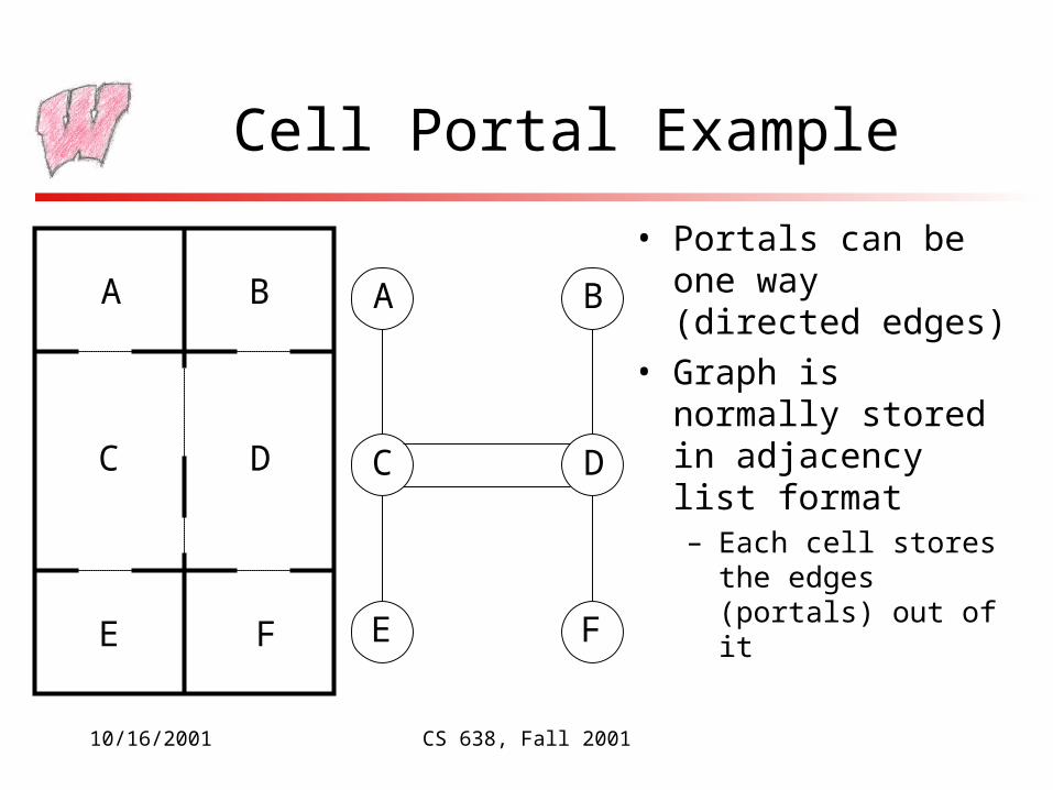
Cell Portal Example

• Portals can be one way (directed edges)

• Graph is normally stored in adjacency list format– Each cell stores the

edges (portals) out of it

A B

C D

E F

A B

C D

E F

10/16/2001 CS 638, Fall 2001

Cell-Portal Visibility

• Keep track of which cell the viewer is in

• Somehow walk the graph to enumerate all the visible regions– Can be done as a preprocess to identify the potentially visible set (PVS)

for each cell• Cell-to-region visibility, or cell-to-object visibility

– Can be done at run-time for a more accurate visible set• Start at the known viewer location

• Eye-to-region or Eye-to-cell visibility

– Trade-off is between time spent rendering more than is necessary vs. time spent computing a smaller set

• Depends on the environment, such as the size of cells, density of objects, …

10/16/2001 CS 638, Fall 2001

Potentially Visible Sets

• PVS: The set of cells/regions/objects/polygons that can be seen from a particular cell– Generally, choose to identify objects that can be seen– Trade-off is memory consumption vs. accurate visibility

• Computed as a pre-process– Have to have a strategy to manage dynamic objects

• Used in various ways:– As the only visibility computation - render everything in the PVS

for the viewer’s current cell• LithTech’s visibility strategy (cell-to-region, as far as I can tell)

– As a first step - identify regions that are of interest for more accurate run-time algorithms

10/16/2001 CS 638, Fall 2001

Cell-to-Cell PVS

• Cell A is in cell B’s PVS if there exist a stabbing line that originates on a portal of B and reaches a portal of A– A stabbing line is a line segment intersecting only portals

– Neighbor cells are trivially in the PVS

I J

H

GA

CB E

F

D

PVS for I contains:B, C, E, F, H, J

10/16/2001 CS 638, Fall 2001

Finding Stabbing Lines

• In 2D, have to find a line that separates the left edges of the portals from the right edges– A linearly separable set problem

solvable in O(n) where n is the number of portals

• In 3D, more complex because portals are now a sequence of arbitrarily aligned polygons– Put rectangular bounding boxes

around each portal and stab those– O(nlogn) algorithm

L L

LLR

R

R

R

10/16/2001 CS 638, Fall 2001

Stab Trees

• A stab tree indicates:– The PVS for a cell

– The portal sequences to get from one to the other

• Used in further visibility processing– Restricts number of

cells/portals that must be looked at

A

C

DE

A/C

C/D1

C/D2C/E

A B

C D

E F

D

F

D/F

10/16/2001 CS 638, Fall 2001

Why Use Cell-to-Cell?

• Most algorithms go further than just cell-to-cell visibility– It overestimates by quite a lot – gets rid of approx 90% of the

model, when in some cases 99.6% is actually invisible, and better visibility gets rid of 98% (Teller 91)

– Cost/benefit favors more time on visibility

• But, keeping cell-to-cell visibility is good for dynamic objects– It is best to track which cell a moving object is in

• Cells are static, and don’t change with the viewer location

• More on updating this information near the end of the semester

– Draw a moving object if the cell(s) it is in is/are visible

10/16/2001 CS 638, Fall 2001

Why not use Cell-to-Cell?

• Problems:– Marks all of a cell as potentially visible, even if only a

small portion is potentially visible• Not good if we are going to list potentially visible objects –

have to list all objects in the cell

– Does not take into account the viewer’s location, so reports things that the viewer cannot possibly see

• More processing can fix these things

10/16/2001 CS 638, Fall 2001

Cell-To-Region Visibility

• Identify which regions are visible from some point within a cell– Then, generally, add objects within region to PVS as a preprocessing

step– Only render objects in PVS for viewer’s cell at run-time

• Key idea is separating planes (or lines in 2D):– Lines going through left edge of one portal and right edge of the

other, and vice versa– In 3D, have to find maximal planes (those that make region biggest)

This picture should remind you of something (Hint: Think of the left portal as a light source)

10/16/2001 CS 638, Fall 2001

Cell-To-Region (More)

• If the sequence has multiple portals:– Find maximal separating lines

• This work originates from many sources, including shadow computations and mesh generation for radiosity

• More applications of separating and supporting planes later

10/16/2001 CS 638, Fall 2001

Enhancing Cell-to-Anything

• If the viewer cannot go everywhere in the cell, then and cell-to-something visibility will be too pessimistic

• One solution is to add special cells that the viewer can see into, but can’t see out of– Put them in places that the viewer cannot go, but can still see

• Above a certain altitude in outdoor games

• Below the player’s minimum eye level

– Basically implemented as one-way portals• The portals only exist in the direction into the cell

– Note, doesn’t work if the player should be able to see through

– LithTech calls them Terrain Hulls

10/16/2001 CS 638, Fall 2001

Run-Time Visibility

• PVS approaches are entirely pre-processing– At run time, just render PVS

• Better results can be obtained with a little run-time processing– Sometimes guided by PVS

– It appears that most games don’t bother, the trade-off favors pre-processed visibility and over-rendering

• At run time the viewer’s location is known, hence Eye-to-Region visibility

10/16/2001 CS 638, Fall 2001

Eye-to-Cell

• Recall that finding stabbing lines involved finding a line that passed through all the portals

• The viewer adds some constraints:– The stabbing line must pass through the eye

– It must be inside the view frustum

• The resulting problem is still reasonably fast to solve– Results in knowledge of which cells are visible from the eye

– Use the stab tree from the PVS computation to avoid wasting effort

– Further optimization is to keep reducing the view frustum as it passes through each portal, which leads us to…

10/16/2001 CS 638, Fall 2001

Eye-to-Region Visibility

• Define a procedure renderCell:– Takes a view frustum and a cell

• Viewer not necessarily in the cell

– Draws the contents of the cell that are in the frustum

– For each portal out of the cell, clips the frustum to that portal and recurses with the new frustum and the cell beyond the portal

• Make sure not to go to the cell you entered

• Start in the cell containing the viewer, with the full viewing frustum

• Stop when no more portals intersect the view frustum

10/16/2001 CS 638, Fall 2001

Eye-to-Region Example (1)

View

10/16/2001 CS 638, Fall 2001

Eye-to-Region Example (2)

10/16/2001 CS 638, Fall 2001

Implementation

• Each portal that is passed through contributes some clipping planes to the frustum– If the hardware has enough planes, add them as hardware clipping

planes

– Or, clip object bounding volumes against them to determine which objects to draw

• Mirrors are reasonably easy to deal with– Flip the view frustum about the mirror

– Add appropriate clipping planes to make sure the right things are drawn

• A very effective algorithm if the portals are simple

10/16/2001 CS 638, Fall 2001

No Cell or Portals?

• Many scenes do not admit a good cell and portal structure– Scenes without large co-planar polygons to act as

blockers or cell walls– Canonical example is a forest – you can’t see through it,

but no one leaf is responsible

• What can we do?– Find occluders and use them to cull geometry– Inverse of cells as portals: Assume all space is open and

explicitly look at places where it is blocked

10/16/2001 CS 638, Fall 2001

Using Occluders (Gems Ch 4.8)

• Assume the occluder is a polygon– If not, use silhouette of object

• Form clipping planes using the eye point and the polygon edges– Supporting planes

• Objects inside all of the occluder’s clipping planes are NOT visible– Occluder itself is a clipping plane– Can use tests similar to view frustum

culling, but note that now we trivially accept as soon as the object is outside a clipping plane

eye

occluder

supporting planes

10/16/2001 CS 638, Fall 2001

Finding Occluders

• Occluders are normally found in a preprocessing step– Identify sets of occluders with regions of space

– At run time, use occluders from the viewer’s region

• What makes a good occluder?– Things that occlude lots of stuff

– What properties will a good occluder have?

10/16/2001 CS 638, Fall 2001

Occluder Issues

• Works best when there are large polygons close to the viewer– Dashboards are a good example

• Objects can be fused to form large occluders– Fuse many tree billboards to form a larger occluder– Put the occluding polygon behind the original polygons– In other words, the occluding polygons can be specially created and

positioned by a level editor• Each occluder good for only a limited range of motion

• Problem: If an object is partially hidden by one occluder, and partially by another, it is hard to determine whether the entire object is occluded

10/16/2001 CS 638, Fall 2001

Combining Occluders

• Using multiple occluders to hide one object is an active research problem– Green’s Hierarchical Z-Buffer builds occluders in screen space and

does occlusion tests in screen space• Requires special hardware or a software renderer

– Zhang et.al. Hierarchical Occlusion Maps render occluders into a texture map, then compare objects to the map

• Uses existing hardware, but pay for texture creation operations at every frame

• Allows for approximate visibility if desired (sometimes don’t draw things that should be)

– Schaufler et.al. Occluder Fusion builds a spatial data structure of occluded regions