The Economic Origins of Democracy Reconsidered

John R. Freeman

University of Minnesota

Dennis Quinn

Georgetown University

10 November 2008 (v2)

Draft – comments welcome

The first version of this paper was presented at the Annual Meeting of the American Political Science Association, Boston, August 28, 2008. We thank James Galbraith, Irfan Nooruddin, Pietra Rivoli, and Vineeta Yadav for comments and suggestions. The paper also benefited from comments at a presentation at the Political Economy working group series at Georgetown. The authors thank Naphat Kissamrej, Dafina Nikolova, Erica Owen, and Ravi Tayal for excellent research assistance. We thank Aart Kraay for discussions of the inequality data sets available, and Keith Ord for advice on the research design. Sections of this paper draw on work done jointly in other projects with Manmohan Kumar and Hans-Joachim Voth.

ABSTRACT

The effect of economic changes sparked by globalization on democracy and

autocracy is a central research question in the social sciences. We review the prevailing

arguments about the links among inequality, financial integration and democratization,

focusing in particular on the contributions of Acemoglu and Robinson (2006) and Boix

(2003). In contrast to the arguments of these scholars, we propose that, because financial

globalization is associated with increasing income inequality and increasing capital

taxation, the relationship between inequality and democratization is a “U.” Countries

with lower and higher levels of income inequality are more likely to democratize. Our

test employs the most current and reliable income inequality and financial globalization

measures available. Despite employing the same design as Acemoglu and Robinson

recently employed in Acemoglu, Johnson, Robinson, Yared (2008), we find no support

for Acemoglu and Robinson’s main causal claims. Rather the hump-shape predicted by

Acemoglu and Robinson or the declining linear relationship in Boix (2003), we find a U-

shaped pattern between these inequality and democratization. We also find little support

for the claim that financial globalization promotes democracy either directly or indirectly.

In fact, contrary to Acemoglu and Robinson and Eichengreen and Leblang (2008), we

find that more inward capital account openness produces lower levels of democratization.

2

The economic origins of democracy and dictatorship continue to be debated. A

prominent theme is that a society’s level of income inequality, joined to elite and citizen

expectations about how political liberalization will influence future changes in income

inequality, are important determinants of political liberalization or retreat.

One well-developed argument is that transitions to democracy are most likely to

occur under moderate levels of income inequality. Democracies are also more likely to

consolidate when income inequality is moderate as well. Democracy is a credible

commitment to income distribution and so, when the poor demand (enjoy) democracy,

they are, in effect demanding (realizing) a change in income inequality. How elites

respond to this demand then determines whether a transition (coup) occurs. Because of

the way international financial globalization affects factor prices, it and other forms of

economic globalization supposedly enhance the prospects for democracy. To be more

specific, financial openness increases wages. This makes the median voter prefer lower

taxes. At the same time, financial integration enhances the ability of elites to exit the

government’s jurisdiction; knowledge of this fact, presumably leads the median voter to

moderate her preferred tax rate. A recent version of this argument can be found in the

book by Acemoglu and Robinson, Economic Origins of Dictatorship and Democracy

(2006; AR hereafter). It was anticipated by Midlarksky (1999).1

A second well-developed argument is that transitions to democracy are most

likely to occur under low levels of income inequality because lower levels of income

inequality reduce the redistributive impact of democracy. While this line of argument has

1 The argument that the origins of democracy can be traced to income and other forms of inequality has been around for many years. T.H.Marshall made an argument of this kind to explain the piecewise extension of democratic rights and privileges in Western societies.

3

a long antecedence, a recent statement with important analytic developments of this

argument is Boix, Democracy and Redistribution (2003).2 As with AR, Boix proposes

that capital mobility (as the term is defined) enhances democratic prospects by limiting

the ability to tax assets of either the ruler or the voters.

The implication in both arguments is that economic integration – particularly

financial globalization – is a force for both democratization and democratic

consolidation. As autocracies become more financially open to inward and outward

capital flows, they ought to be more likely to democratize. Similarly, financial and other

forms of economic integration should help young democracies consolidate. The

mechanism at work in both AR and Boix is that highly mobile capital assets are

somewhere between lightly taxed and untaxed because, with capital mobility, mobile

capital assets will be located in countries offering “tax havens.” With the decreasing

ability to tax (and hence redistribute) wealth from capital, the costs of democracy

decrease, and elites are more likely to accept democratization.

Recent results by Eichengreen and Leblang (2008) offer support for this

perspective. While Eichengreen and Leblang do not explicitly examine the democracy

and inequality linkage, they do find that capital account openness is strongly associated

with subsequent democratization.

Our paper offers a revised theory regarding relationships among inequality,

financial globalization, and democratization, and tests this and other theories. Our test

employs the soundest and most current income inequality and financial globalization

measures available. The investigation is divided into three parts. We begin by briefly

2 Aristotle (Politics, Book V) is of course the progenitor of most of the “materialist” arguments about how desire for changes in the distribution of wealth within a polity spawned revolution and political turmoil.

4

reviewing and critiquing the prevailing arguments about the link between inequality and

financial integration and democratization, in particular the contribution of Acemoglu and

Robinson (2006) and Boix (2003). In the process, we illuminate several causal linkages

that must exist if their thesis is to hold. We propose that, because financial globalization

has effects on income inequality contrary to those proposed in Acemoglu/Robinson and

Boix, countries with lower and higher levels of inequality are likely to either democratize

or consolidate democracy. Given financial globalization, it is countries with intermediate

levels of inequality, we propose, that are less likely to democratize.

Part two of the paper takes up the relevant measurement issues, especially the

difficulties associated with gauging income distribution cross-nationally. Within this

section, we also discuss some specification and estimation issues. In the end, we settle on

essentially the same research design employed by Acemoglu, Johnson, Robinson and

Yared in the recent article on income and democracy (2008).

The results are presented in part three. Simply put, despite the fact that we employ

the same design as they recently employed (ibid), we find no support for Acemoglu and

Robinson’s main causal claims. We do not find that the intermediate ranges of income

inequality promote democracy. Rather than the hump-shape predicted by Acemoglu and

Robinson or the downward sloping line predicted in Boix, we find a U-shaped

relationship between these inequality and democratization. We also find little support for

the claim that financial integration promotes democracy either directly or indirectly. In

fact, contrary to Acemoglu and Robinson and Eichengreen and Leblang 2008, we find

that capital account liberalization is negatively associated with democratization.

5

The Microfoundations of the Arguments3

The arguments of AR and Boix are similar, though their conclusions differ. AR

partition society into two groups, the poor and the rich (p, r), an architecture that Boix

2003 closely follows from earlier AR published work.4 The poor outnumber the rich by

a considerable margin.5 The two groups have complete information. They struggle over

the distribution of resources; redistribution is accomplished by means of a common

proportional tax, the proceeds of which are transferred (in equal shares) to all members of

society. Democracy is an institution that makes commitments to redistribution more

credible than the promises to redistribute by the rich (in autocracy). The questions are: 1)

Do the poor accept the policies and promises offered by the rich or do they choose to

revolt?; and, concomitantly, 2) Do the rich offer tax rates that are their most preferred

policy (zero taxation), “concessionary” rates that are nonzero but also not the rates most

preferred by the poor, or choose to democraticize?

AR and Boix use game theory to derive the best responses (strategies) of the rich

and poor under a variety of conditions pertaining to democratic and autocratic societies.

Their account of democracy is based on previous work by Meltzer and Richard (1981)

and others.

The core intuition is that the median voter’s preferences are determinative, and

that the median voter is a poor individual. Her most preferred tax policy takes into

account the deadweight loss of taxation, C(τ). But, even then, unlike the rich, she still

3 In the interest of brevity we focus here on the explanation of the transition from autocracy to democracy. There is a parallel argument concerning democratic consolidation. 4 See AR 2006, p. 87 for a discussion of the relationship of their work to Boix’s., and see Boix 2003, p. 11, for a discussion of the relationship of his work to theirs. 5 In several places in their book AR consider more complex partitionings of society, including the possibility of a middle class. But their core argument is framed in terms of a distributional struggle between the poor and the rich.

6

favors a nonzero tax rate, τp. Moreover, her preferred tax rate increases with the level of

inequality in society; mathematically, this follows from the assumption that the share of

income held by the rich, θ, is greater than the share of the population that is poor, δ.

Therefore, in democracy, the median voter’s preferences are always implemented and

this leaves the poor better off and the rich worse off in terms of post-tax income.6

The situation in autocracy is a bit more complicated. AR’s most simple static set-

up implies that the rich have a choice between imposing a tax rate that is no better than τp

or suffering a revolution and losing all their wealth. For their part, the poor must choose

between accepting the tax rate imposed by the rich or opting for revolution. A key

assumption regarding the latter option is that revolutions destroy forever a share of

societal resources, μ. This means that after the revolution, while the rich have no income,

the poor earn a reduced rate than what would be possible in a democracy where the

preferences of the (poor) median voter were adopted.7 So, for the poor, the question, in

the simplest static model, is whether their post tax income is higher under the tax rate

offered them by the autocratic rich relative to the post tax income they would obtain after

losing a share of societal resources in the revolution. This is called the revolutionary

constraint. AR show it is equivalent to the condition θ> μ.8

6Pre tax incomes of the two groups are expressed as yp = [(1-θ) y /(1-δ)] and yr = (θ y )/δ where θ is the share of the income accruing to the rich, δ is the fraction of the population that is rich (assumed to be less than .50), and y is the average income of individuals in the society. Post tax income is expressed as V(yi | τ) = (1 – τ) yi + T = (1 – τ)yi + (τ – C(τ)) y where V denotes indirect utility, yi is the income of individual i, τ is the tax rate, T is the transfer (from government collected taxes), C(τ) is the deadweight loss of taxation, and y is defined as before. AR show that the derivative of τp with respect to the level of inequality in society, θ, is positive. 7 That is, after revolution the payoff to the rich, Vr(R,μ) = 0 and the payoff to the poor is Vp(R,μ)= [(1-μ) y ]/(1-δ) where μ is the share resources destroyed forever by the revolution, y is average societal income and δ is the share of the population that is poor. 8 This derives from the condition Vp(R,μ) > yp.

7

Democratization occurs when revolution is relatively more attractive to the poor

than the concessions the rich might offer and, for the rich, repression is more costly than

democratization.9 Given these results, AR then show that democratization is likely only

under intermediate levels of inequality, θ. For low levels of θ, revolution is not a viable

option for the poor. Hence, the rich may be able to implement their most preferred tax

policy and; therefore, autocracy survives. Above a certain high threshold level of θ, elites

have more to lose from democracy than they do from repression (or from concessions).

The rich, therefore, opt for repression and all agents suffer a loss in income. But this

leaves the rich relatively better off than they would be if they agreed to democracy and

the poor were able to choose their most preferred tax policy.10

AR produce causal propositions. The one they most highlight is:

AR Proposition 1. There is a (convex) hump-shaped relationship between societal inequality and democratization within and across countries.

Boix argues that lower levels of inequality or increasing capital mobility lead to

democracy: “democracy prevails when either economic equality or capital mobility are

high in a given country.” (2003, 3.) With lower levels of inequality, elites have fewer

incentives to resist democracy as the costs of redistribution are lower.

9See Proposition 6.2, AR p. 189. 10This essentially is AR’s Corollary 6.1. To derive this key corollary, AR examine the conditions relative to θ, that (the promise of) concessionary taxation is just enough to prevent revolution, the condition relative to θ under which the value of democracy is equal to that of revolution for the poor. They show there is a range of inequality levels where democracy can be be conceded by the rich, the rich end up better off than if they had repressed (given the value of the cost of repression) and the poor do are satisfied with the tax policy of the median voter. There is, however, an upper threshold in equality that produces democracy, however. Beyond this upper threshold, democracy—the tax policy of the median (poor) voter—leaves the rich worse off than they would be under repression. Put another way, at this upper level of inequality, the cost of repression has to be very high before the rich would opt for democratization. At this upper level, either a) (promises of) concessionary taxation don’t work, the poor prefer revolution, and repression is the only option for the rich (to avoid a total loss of income) or b) the poor prefer democracy to revolution, but the rich still are better off repressing the poor than agreeing to democracy and accruing the post-tax income produced by the tax policy of the median (poor) voter, τp.

8

How does economic globalization figure in the microfoundations of these

arguments? International economic forces further enhance the prospects for

democratization for both sets of scholars. AR assume that in most autocratic countries

labor is abundant and capital is scarce. They also assume that trade encourages factor

price equalization. The result is an increase in the returns to poor--an increase in the

poor’s income--and a reduction in the poor’s preferred tax rate. After trade, a relatively

lower income loss to the rich relative to the poor is sufficient to make democracy the

preferred choice over repression (because democracy means a higher post-tax income

when the poor (median voter) chooses the lower, post trade tax rate).

Capital mobility supposedly has some of the same effect as trade on the prospects

for democratization. Capital inflows occur, before financial integration, in developing

countries, because the return to capital is higher domestically than internationally;

eventually these rates of return are assumed to equalize at which point capital inflows

stop. The equalization (increase) in wage rates occurs at the same time and, again, this

lowers the preferred tax rate of the poor, making democracy relatively more attractive

than repression. This impact on wage rates is sufficient to make democracy more likely.

One reason is that, in their analysis of the inflow case, AR assume there are no local taxes

on foreign capital and no taxation of capital abroad.11

In regards to capital outflows, AR assume a global (post-tax) rate of return on

capital that is higher than the domestic (post-tax) return. They contend that, in

11 AR also assume no cost to foreign capital from coups. They do not say if there is a cost to foreign capital from revolution. It appears this cost also ruled out by AR. This argument about capital inflows is for the developed country case. In the opening to the chapter on opening economies, AR point out that effects on wages and on capital are reversed in developed countries. In this case, wages fall and the returns to capital rise. But since these countries have “fully consolidated democracies” the implied, resulting “marginal increase in redistribution” will not provoke a coup. In other words, parameter values depend on the duration of democratic consolidation (see AR p. 323).

9

democracy, the poor are forced to equalize the two rates, or capital will flow out of the

country (reducing post-tax income). As with trade, this lowers the preferred tax rate for

the poor (median voter) to some τ p < τp. This, again, makes the payoff of democracy

relatively higher to the rich than it would be without capital outflows. In turn, repression

is less attractive. To be more specific, with capital outflow, repression has to be cheaper

(because there is less of an income loss) for it to be preferred by the rich. Thus,

democratization is encouraged by capital outflows.

AR’s analysis of the impact of economic openness on democratization produces a

clear causal expectation:

AR Proposition 2. In developing countries, both inward capital account liberalization and outward capital account liberalization lead to democratization though the mechanisms differ; inward liberalization leads to reductions in inequality, and outward liberalization limits redistributive taxation.

Boix does not discuss financial globalization in the more traditional sense of

either capital account deregulation or inward and outward capital flows. Instead, Boix

focuses on “the specificity of capital,” which is “a reduction a reduction in the cost of

moving capital away from its country of origin.”12 (2003, 12.) The less “specific” the

asset, the more mobile is capital. The link between lower asset specificity (capital

mobility) and democracy is straightforward:

….this book predicts that a decline in the extent to which capital can be either taxed or expropriated as result of its characteristics also fosters the emergence of a democratic regime. As the mobility of capital increases, tax rates necessarily decline since otherwise capital holders would have an incentive to transfer their assets abroad.

12 Readers of the literatures in international business and foreign direct investment will note immediately that scholars in these fields see the international investment assets of globalized firms as being highly specialized and “specific,” far more so than investments of purely domestic firms.

10

The “specificity” of an asset for Boix depends on its value outside the country of origin:

…capital can be thought of as being somewhat specific to the country in which it is being used. The extent to which an asset is specific is measured by its productivity at home relative to its productivity abroad. Whenever capital is moved abroad, it loses a share (σ) of its value. More exactly, capital k, which at home would produce y=k, produces abroad y=k(1- σ). Thus, the more specific the capital, that is the larger the σ, the less attractive the option of moving capital abroad becomes to its owners. The degree of specificity varies across types of capital: it is practically complete for land, yet extremely low for money or generic skills. (2003, 12)

As less specific assets are harder to tax, lower redistribution possibilities come with them,

as does greater likelihood of democratization.

Recent studies of this subject by other scholars are noteworthy for their focus on

the related, but different argument that it is capita income levels and GDP growth that

determine democratization and consolidation (Barro 1999, Boix and Stokes 2003, Epstein

et al 2006, Acemoglu, Johnson, Robinson, and Yared 2008). The use of income equality

occasionally is included in the robust checks for the models relating income levels

(growth) to democratization. This variable, however, is typically omitted. Sometimes the

investigator says he would like to include income equality in the democratization

(consolidation) model but data paucity prevents this (Svolik, 2008, 165).13

Of course a few scholars have examined the relationship between foreign investment and

income equality. The results of their investigations, however, are contradictory.14

13 Barro (1999, S169-171) includes income and educational inequality in the robustness checks for his SUR model relating income levels and growth to democratization. He finds only weak evidence of relationships for this inequality measures. Acemoglu, Johnson, Robinson and Yared (2008) show Barro’s model is sensitive to the omission of fixed effects and some forms of endogeneity. AR cite the study of Epstein et al as support for their nonmonotonicity result (p. 193). But this is the working paper version of the Epstein et al. The published version of Epstein et al (2006) does not use income inequality as a regressor in explaining democratic transitions and(or) consolidations. 14Jensen and Rosas (2007), in a study of the Mexican experience find direct foreign investment (DFI) reduces income inequality. In cross-national, pooled analysis of a collection of 69 countries, Reuveny and

11

Evaluation and Hypothesis Development

Both main arguments about the link between income inequality and

democratization (democratic consolidation) rest on empirical footing worthy of

reinvestigation, and on theoretical assumptions that are debatable. We focus in particular

on four elements: 1) the absence of empirical support for AR’s argument; 2) the

possibility of endogeneity in relationships; 3) the role of financial globalization in

influencing the democracy and inequality relationships; and 4) the soundness of the

assumption about capital taxation under conditions of financial globalization. We

propose that financial globalization has effects on income inequality such that

inequality’s effect on democratization is non-linear and “U” shaped – more equal and

highly unequal societies are more likely to democratize or consolidate democracies than

are nations characterized by intermediate levels of inequality.

Evidence. Little meaningful evidence has been provided in support of the AR argument

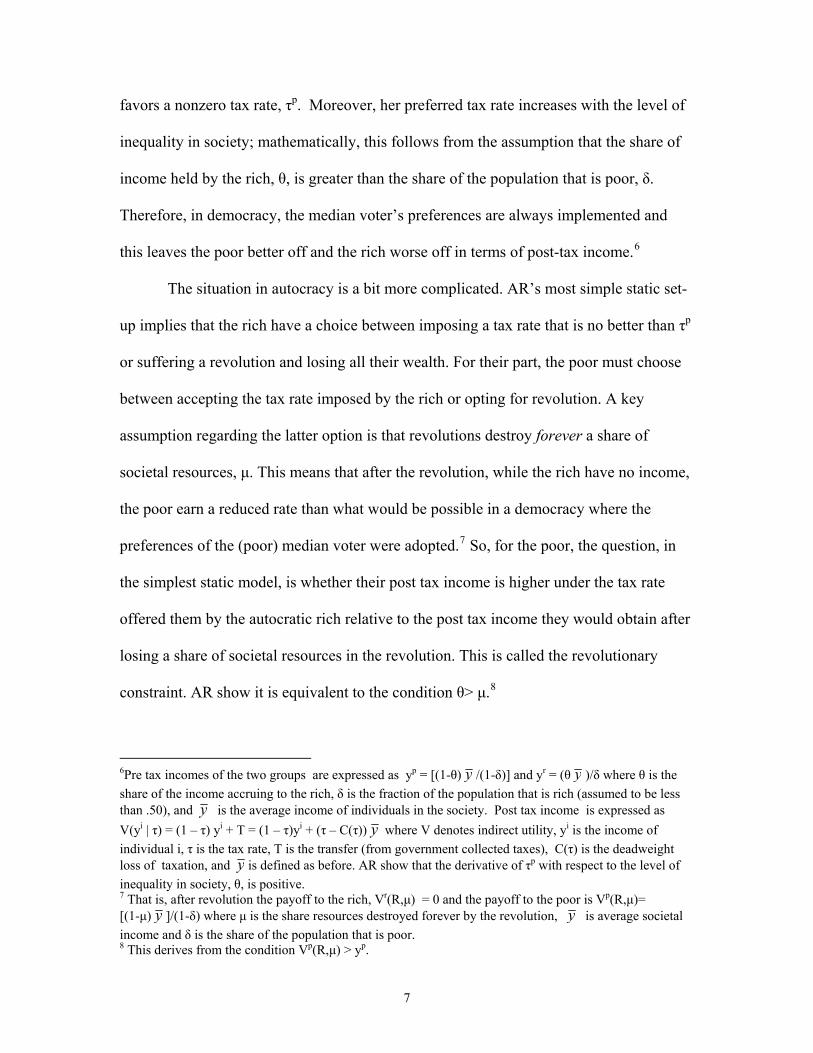
in particular. AR offer a few scatterplots in support of the idea that income inequality

and democracy are correlated (Figure 1). These scatterplots, however, actually show a

curiously monotonic relationship (even though their central thesis is that the relationship

is nonmontonic).15 In fact, the relationship in AR’s Figure looks more like that predicted

by Boix (2003). At no other place in their book do they produce any statistical analysis in

support of their argument. In fact, in their analysis of the impact of international

Li (2003) found democracy and trade reduce income inequality, DFI actually increases income inequality, and “finance capital” had no effect on income inequality. 15Later, in Chapter 6, AR report data on a single downturn in inequality in Korea-Taiwan and of a relatively flat trend in income inequality in Singapore (Figure 6.3, p. 192) as evidence of the nonmonotonic relationship. Needless to say, these data do not support the strong claim they make about nonmonotonicity. Below, we review the logic behind the thesis that income inequality of intermediate levels is only likely to produce democracy (2006, p. 37, 189-193).

12

economic forces on inequality and democracy, they admit that the evidence is “unsettled”

or “equivocal” (2006, 344-5, 347; see also 325).

Figure 1 Acemoglu and Robinson’s (2006) Figure 3.16

The results obtained from the simple correlational (graphical) approach used by

AR are not reassuring. For example, scatterplots for our most current data on income

inequality and changes in polity scores show no clear relationship (Figure 2). The

coefficients on contemporaneous and lagged Gini variables raised the second and third

13

powers in regressions explaining changes in Polity scores are statistically insignificant at

conventional levels.16

Figure 2 Lagged Gini Scores and Change in Polity Scores for 424 Country Years

Endogeneity. Another concern is the possibility of endogeneity. Consider the following

schematic representation of the argument in AR’s tenth chapter linking financial

openness to democratization:

16AR (2006, p. 59) use Dollar and Kraay’s (2002) data for their Gini scores. As we explain below, our Gini data subsumes the Dollar-Kraay Gini scores as well as several more recent income inequality data sets. As regards the simple regression analyses, we estimated models with Gini scores squared and squared and cubed. We used both contemporaneous average Gini scores and lagged average Gini scores. None of the coefficients in these simple regressions were statistically significant at the .05 level. In a parallel analysis using a lagged endogenous variable for change in democracy, time dummies we also found no statistically significant curvilinear relationship. This supplemental analysis used several measures of democracy and all five our measures of inequality. See Appendix (August 12 email).

14

This causal chain is a recursion and therefore relatively easy to estimate. But, if

the causal arrows point in both directions, the estimation obviously will be more difficult.

In particular, endogeneity will be an issue. And there are many places in AR’s analysis

that suggest endogeneity is present. One is their analysis of the impact of concessionary

taxation in autocracy; concessionary taxation may affect income inequality.17 Statistical

tests therefore not only must “control” for the variables left out of AR’s analysis but also

17 AR treat the level of income inequality in autocracy as exogenous, fixed parameter. Yet one of their main insights is that the rich, under certain conditions, can (promise to) redistribute some income to stave off revolution; this rate is expressed in equation (2) in the text. How this concessionary taxation affects the level of income inequality is not clear. In addition, AR go back and forth—sometimes even in the same passage (e.g., p. 189) between talking about the promise to redistribute income via concessionary taxation and the actual redistribution of concessionary taxes. They also do this in their dynamic analysis (pps. 198-199). Once more, how concessionary taxation and redistribution could leave θ unaffected is not explained. Another likely form of endogeneity is the relationship between capital outflows and the size of the capital stock. The loss of capital in this case may have the same impact as the loss of capital due to revolution or coups.

15

estimation must take endogeneity into account. Unfortunately, AR give us little guidance

how best to accomplish these things.

Please see the technical appendix for further evaluation of the AR model. We

endeavor in this paper to evaluate empirically their argument, taking particular note of the

differing theorized effects of inward and outward capital on inequality and hence

democracy.

Boix 2003 offers more systematic tests of his argument. Using panel methods and

simple maximum likelihood estimation, Boix (2003, 79-83) generally finds negative

associations between inequality as an independent variable and subsequent

democratization.

The models and tests did not allow, however, for estimation of the necessary

endogeneity in relationships in both the AR and Boix arguments.18 In Boix (as with AR),

the core argument is that it is actor expectations about how elites and “masses” pursue or

resist future democratization in light of their preferences regarding current and future

distributions of income that influence the likelihood of a country’s democratization.

Therefore, expectations of about future democracy potentially influence current

distribution of resources; and, expectations about future democracy influences

expectations about future income distribution, all of which in turn is correlated with

current distribution.

Note that many papers explicitly reverse the dependent and independent variables

in the AR and Boix investigations, and instead model the effect of democracy and

18 Boix acknowledges that the democracy and inequality variables are endogenous, especially in a cross-sectional research design (2003, 74). But, Boix says “even if inequality is an endogenous variable to political regime, it is determined previously to the political game we are playing.” If, as Chong 2004 and others note, independent and dependent variables exhibit persistence over time, an instrumenting procedure is advisable.

16

autocracy on income inequality (Reuveny and Li 2003, e.g.). Some recent papers model

the relationships endogenously; see, e.g., Chong 2004 (especially 193, 203) in which a

GMM_System set-up is used to explore the effects of democracy on changes in

inequality. We propose that an econometric examination of the effects of inequality on

democracy should be undertaken at least in part using some form of instrument variable

regression analysis.

Financial Globalization and Inequality. Capital account mobility’s effect on

redistributive taxation is crucial for Boix as well as for AR. Boix operationalizes asset

specificity, and hence capital account mobility, with indicators of a country’s agriculture

share of GDP, the value of its fuel exports over other its exports, the average years of

schooling of its population, and economic concentration of its markets, as well as

national income.

Capital account mobility, however, is the result of capital account liberalization (a

treatment variable), which produces financial integration (an outcome variable). Both

variables can be measured directly, though neither is evidently measured by the above

indicators.

Capital account liberalization changes the meaning and economic value of “asset

specificity.” With capital account liberalization, capital assets – including land – are no

longer “specific” in an economic sense (cf. Ansell and Samuels 2008). Owners of land

are able to sell property rights to foreigners (who are presumably seeking diversified

portfolios). Those land-owners are able to, in turn, purchase assets in foreign markets.

Argentine landowners, e.g., with capital account liberalization, can sell assets to overseas

investors, and invest the proceeds internationally. Even labor is not quite so “specific” as

17

laborers can sell “labor” to foreign investors, and these workers can invest the returns of

their labor in overseas markets. Capital account liberalization has been a core, if not the

core, contributing factor to asset market integration (Quinn and Voth 2008).

Indeed, insuring that that an investor’s assets are not too “specific” (or, more

correctly, not too idiosyncratic in risk) is the key recommendation of modern portfolio

theory - international diversification, in particular, is good for investors. A long lineage of

work, starting with Henry Lowenfeld, in his The Geographical Distribution of Capital

(1909) demonstrates that international equity market correlations are lower than industry

correlations within one country. Consequently, investors should be able to improve the

risk/return profile of their portfolio significantly if they move assets out of “specific”

classes of investments, and partly into foreign equities and assets (Grubel (1968), Levy

and Sarnat (1970)). Paradoxically, with capital account openness, specific assets (or

those that have idiosyncratic risk that are uncorrelated with returns in global capital

markets) become highly valuable to foreign investors as components of a diversified

portfolio.

Hence, we expect that, following capital account liberalization, local investors

will see high returns through asset sales to foreigners, which will increase – not decrease

– income inequality. And, assuming that capital account liberalization limits, a la both

AR and Boix, “excessive” taxation of investor gains, this increase in inequality will be

extensive.

Empirical studies offer some evidence that financial globalization will lead to

increasing income inequality. Financial globalization was found to be a robust correlate

of rising income inequality in a cross-section of countries examined in Quinn 1997. A

18

recent paper by Jaumotte, Lall, and Papgeorgiou (2008) uses panel OLS methods to

disentangle the effects on income inequality of technological innovation, trade, and

financial globalization. They find that, while trade does have the effect of reducing

income inequality, inward FDI flows have increased income inequality. A study in 2008

by the International Labor Organization (ILO) also uses OLS panel methods to document

the correlation between rising income inequality and stock of FDI as a percentage of

GDP (ILO 2008). See also Figini and Görg (2006), which show initial rises in wage

inequality from inward FDI.

Financial globalization, we propose in this light, will have complex effects on

democratic prospects – rising inequality will hurt democratic prospects, but limits to the

taxing of the rising inequality should lessen elite opposition to democratization. Hence,

the relationship among financial globalization, rising inequality, and democratic

prospects is likely to be non-linear.

Financial Globalization and Capital Taxation. A key assumption in both AR and Boix

is that capital is either not taxed (i.e., inward investment by non-residents) or taxed at low

rates (~a low global rate of taxation). These assumptions are consistent with standard

predictions from small, open economy macro models, which have long suggested that

capital and corporate taxation in smaller economies with open capital accounts are

difficult to sustain, and are vulnerable to a “race to the bottom.” (See Devereux,

Lockwood, and Redoano 2007 and Tanzi 1995 for models. See Haufler 2001 for a

review.) The prediction of the open capital accounts models is generally that a

government’s revenue from capital taxation disappears, even if governments persist in

maintaining tax rates.

19

Paradoxically, in the models advanced in AR and Boix, the unsustainability of

high levels of taxation on mobile capital with open capital accounts is good news

normatively for democracy; without revenue to redistribute, democracy becomes less

costly to the elite, and opposition to democracy becomes more limited. This “good

news” is a reversal of sorts of earlier arguments made in political science that open

capital accounts limit democratic choice.

It is difficult, however, to think of an area of international political economy

research that has produced predictions more at odds with the observed behavior of

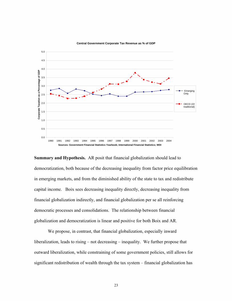
governments and economic actors. Consider Figures 4, 5, and 6.19 Figures 4 and 5

report OECD corporate tax collections and rates for 1970 and 2005, both years of world

business cycle expansion.20 For the average OECD country, corporate tax revenues as a

percentage of GDP have risen in the past 35 years from 2.5% of GDP to 3.6%; the 35

years between 1970 and 2005 are a period of financial globalization among OECD

countries, with no significant capital controls remaining in 2005. (Similar results are

found for more open emerging market countries from 1960-1989. See Quinn 1997.) Top

corporate tax rates have fallen on average during the same period (see Figure 5), but the

tax base has been broadened through reductions in incentives and other deductions, and

base-broadening has contributed to the steep rise in corporate tax collections. (See

Devereux, Griffith, and Klemm 2002 for a review of the policy debate around cutting top

tax rates while “tax-base broadening.” See also Swank and Steinmo 2002.) Emerging

19 We use corporate capital taxation (revenue and rates) as our proxy for capital taxation. Data on corporate taxation is reliable, in contrast to data for the more general category, “capital” taxation. What constitutes “capital” income varies extensively cross-nationally, in contrast to corporate income. 20 Because taxation is frequently counter-cyclical, controlling for stages of the business cycle is important in analysis over time. Both 1970 and 2005 were part of peak world business cycles, with world growth averaging 5% both year. See IMF, World Economic Outlook, April 2007, p. 1.

20

market corporate tax collections (Figure 6) in recent year have not grown, in contrast to

collections for OECD member countries, but they have remained relatively stable.

Addressing the discrepancy between theory and evidence in a paper entitled

“Why is there no race to the bottom in capital taxation?,” Plümper, Troeger, and Winner

(forthcoming) argue that fiscal rules and equity norms (measured by Gini coefficients)

put upward pressure on capital taxation, both rates and revenue. While “tax competition”

does cause some shifting of tax burdens to less mobile factors, fiscal rules and social

fairness norms trump. Their model and results confirm that countries with open capital

account do not converge on capital tax policies in general, and do not “race to the

bottom” in particular. Their findings are consistent with the “system of constraints”

argument and evidence in Swank and Steinmo (2002) and the “tournament” model in

Basinger and Hallerberg (2004). See also Countries, while not free in these analyses to

tax capital at confiscatory rates, are able to capture substantial income from capital

taxation under conditions of capital account openness.

The implication we draw is that governments are able to extract substantial

revenue from owners of capital assets under conditions of financial openness. Financial

globalization does not necessarily eliminate the tax burden on capital, and does not

necessarily reduce the incentives of elites to resist democracy. Indeed, if financial

globalization increases inequality and allows for redistribution, financial globalization

under some conditions might increase an elite’s resistance to democratic reform.

21

Figure 4 - OECD Corporate Tax Revenue Collections as % of GDP - 1970 vs. 2005

0

1

2

3

4

5

6

7

Greece

Denmark

Spain

Austria Ita

ly

Finlan

d

Sweden

German

y

France

Belgium

Netherl

ands

Irelan

d

United

King

dom

Austra

lia

New Zea

land

United

States

Canad

aJa

pan

AVERAGE

sources: OECD Revenue Statistics, 1965-2007 (2008 ed.)

Tax

Rev

enue

as

% o

f GD

P

Tax % GDP 1970Tax % GDP 2005

Figure 5 - Central Government Top Corporate Tax Rates - 1970 vs. 2005

0

10

20

30

40

50

60

Italy

Belgium Spa

in

Irelan

d

Greece

Denmark

Japa

n

Sweden

United

King

dom

Finlan

d

Netherl

ands

Canad

a

Austria

Austra

lia

United

Stat

es

New Zea

land

France

German

y

AVERAGE

Sources: OECD, Revenue Statistics, Part II, Table II.1 (2008); KPMG Corporate Tax Rate Survey 2006(note: "combined" corporate tax rates, which include subnational government tax rates, are not shown)

Top

Mar

gina

l Cor

pora

te T

ax R

ate

Tax Rates 1970Tax Rates 2005

22

Central Government Corporate Tax Revenue as % of GDP

0.0

0.5

1.0

1.5

2.0

2.5

3.0

3.5

4.0

4.5

5.0

1990 1991 1992 1993 1994 1995 1996 1997 1998 1999 2000 2001 2002 2003 2004

Sources: Government Financial Statistics Yearbook; International Financial Statistics; WDI

Cor

pora

te T

axat

ion

as a

Per

cent

age

of G

DP

EmergingOnly

OECD (22traditional)

Summary and Hypothesis. AR posit that financial globalization should lead to

democratization, both because of the decreasing inequality from factor price equilibration

in emerging markets, and from the diminished ability of the state to tax and redistribute

capital income. Boix sees decreasing inequality directly, decreasing inequality from

financial globalization indirectly, and financial globalization per se all reinforcing

democratic processes and consolidations. The relationship between financial

globalization and democratization is linear and positive for both Boix and AR.

We propose, in contrast, that financial globalization, especially inward

liberalization, leads to rising – not decreasing – inequality. We further propose that

outward liberalization, while constraining of some government policies, still allows for

significant redistribution of wealth through the tax system – financial globalization has

23

been associated, at least in part, with increasing corporate tax collections. If rising

inequality harms the prospects for democratic consolidation and democratic reform, and

if the “ceiling” on taxation under financial globalization is high, then the financial

globalization→inequality→democracy relationship is likely to be non-linear. We

propose that, as inequality from globalization rises, democratic prospects should

diminish. At some point, however, rising inequality is high enough so that, with financial

globalization and a given ceiling on capital taxation, elites will be less resisting of

democracy. Therefore, we posit a U-shape relationship among financial globalization,

inequality, and democracy.

The next sections describe the data used and put forth such a design. We then

conduct a test of these propositions.

Data and Measures

Data choices significantly influence many scholarly studies. We outline here

some of the choices investigators face in estimating models using measures of

democracy, inequality, and financial globalization. We then assess the consequences of

these choices. Where feasible, we use multiple indicators of key variables.

Democracy. Our core dependent variable in this investigation is democracy, which we

measure by using Polity II and Regime.21 These democracy measures are standards in

political economy. We estimate models using the two variables to demonstrate

robustness of our results. In using the 21 point Polity measure, we allow for minor as well

as major changes in democratic institutions to be modeled. In using the 0,1 Regime

21 Polity II is from Marshall, Jaggers and Gurr 2000 (updated at www.bsos.umd.edu/cidcm/polity). Regime is from Przeworski et al. 2000 (upates available from Cheibub and Ghandi 2004, as cited by http://www.nsd.uib.no/macrodataguide/set.html?id=1&sub=1.

24

variable, we focus on larger changes. (Note that in a five year panel, the dichotomous

Regime variable is transformed into an interval level variable taking values between 0

and 1, and which is continuous and normally distributed). Regime is rescaled so that

large values indicate greater levels of democracy or of civil liberties.

We show below that the choice of the democracy indicator is not per se a crucial

choice in the investigation. Regime, however, has fewer observations than Polity II, and

the end of the respective series coincides with important changes in history. But, regime

ends in 2000, and misses recent events. Polity II covers the period between 1945 and

2004, and therefore contains more identifying variance.

Inequality. In contrast to the democracy indicators, which are broadly comparable across

space and time, the cross-national inequality indicators are plagued with measurement

difficulties. We use as our measure of inequality Gini coefficients22 from three standards

sources: Deininger and Squires 1996 (D&S); Milanovic 2005, and United Nations

University-World Institute for Development Economics Research’s World Income

Inequality Database (WIID) 2008. The D&S and WIID data, however, contain

information from diverse sources using diverse methods on diverse populations. These

data need to be adjusted before using in cross-national, time-series analyses.23 The

Milanovic/World Bank survey data are comparable across time and space, but are limited

in time to at most three observations per country.

22 Gini coefficients are a way of measure a nation’s income inequality. They are scaled between 0-100. Gini coefficients measure the dispersion of income, with high values indicating higher inequality. 23 The main differences are whether surveys measure income or expenditure, households or individuals, and are net of taxes and transfers or are gross income. We use GINI indicators that are a) national in origin, b) are rated as having a WIID quality of at least “3,” and c) where possible, consistent by methodology within country.

25

Dollar and Kraay 2002 (DK) and Babones and Alvarez-Rivadulla 2007 (SIDD)

each offer transforming metrics that allow for the GINI indicators to be turned into

measures useful for comparative research. 24 We use DK’s transformation algorithm to

adjust the 2008 WIID data. As noted below, we find that a third variable (household vs.

person) is influential in the new 2008 WIID; we estimate a transformation with the third

dimension added (FQ3). We also estimate a two variable GINI adjustment model, and

find that the consumption coefficient is larger than the DK adjustment: we refer to this

series as FQ2. While the transforming metrics differ, the intercorrelations between and

among the measures are reassuringly quite high: great than 0.9. (See Appendix Table

A1.) We offer an assessment of whether differences in methodology (as well as

differences in sample size) influence the investigation below.

The Galbraith and Kum 2005 inequality indicator, EHII, uses United Nations

Industrial Organization (UNIDO) wage data with a Theil T’s statistic to generate over

3,000 country year observations of GINI. An advantage of their approach is that a fuller

data set using wage data is estimated. A disadvantage is that their data end in 1999,

whereas the new WIID data extend to 2006. The correlation between EHII and the other

GINI indicators is not high: ~.6. We show below that the results of the investigation

24 Dollar and Kraay 2002 (Table 2) use a regression on GINI using dummy variables for gross income and expenditure (consumption), plus regional dummies. They then subtracted the coefficient estimates of the gross income and expenditure dummies from the GINI coefficient. Identical results are given by extracting the residuals of the regression, and adding them to the intercept. Dollar and Kraay did not use a dummy for household vs. person as they do not find a statistically significant effect (Email correspondence, A. Kraay and D. Quinn, 21 July 2008; phone conversation, 17 July 2008.) We replicate nearly exactly Dollar and Kraay’s results for Table 2 on their sample. In the WIID 2008 updated sample, however, we find that the coefficient estimate for household is now statistically significant, and that the regional dummy effects in Dollar and Kraay are now very different from prior findings. A simple model regressing GINI with dummies for all three types of surveys is what we use. We also estimate a model without the household dummy. The coefficient estimate for expenditure surveys remains consistent with the early Dollar Kraay result, but the coefficient on the gross income dummy is now twice the size as before. We use both results.

26

will sometimes differ, depending on which of these GINI indicators are used. (See the

Appendix Tables A1 and A2, which illustrate the correlations across measures.)

Financial Globalization. We operationalize international financial regulation as two

indicators of change in international financial openness or closure, which are described in

Quinn (1997) and Quinn and Toyoda (2007). CAPITAL and FINANCIAL_CURRENT

(FIN_CURRENT hereafter) are the main components of openness created from the text

published in the annual AREAER volume that reports on the laws used to govern

international financial transactions. These indicators take a different approach in creating

an index for a government’s policy stance toward capital account liberalization and

financial current account liberalization by offering a measure not only of the existence

(absence) of restrictions, but also of the severity or magnitude of those restrictions.

We chose nations for coding based primarily upon how early their information

appeared in AREAER. For example, descriptions of the financial arrangements as of

1949 for 47 nations appeared in the first volume (1950), and all these nations (save three

whose data were subsequently interrupted) appear in the data set. Up through the 1960s,

as other nations entered AREAER, we added them to the data set, which currently

contains information for 111 nations. Our aim has been the “longest t,” rather than the

“broadest N.” CAPITAL is scored 0-4, in half integer units, with 4 representing an

economy fully open to capital flows. This measure is transformed into a 0 to 100 scale by

calculating 100*(CAPITAL/4)

CAPITAL distinguishes between restrictions on residents and non-residents,

which correspond to restrictions on capital outflows and inflows, respectively. (See IMF

(1993), pp. 80-1, for a discussion).

27

To measure a country’s integration into global financial markets, scholars often

turn to non-index, de facto or “blended” measurements. These indices exploit observable

phenomena resulting from increased capital mobility, such as the magnitude of gross

capital flows (IMF 2001), share of domestic equities that are available for foreign

purchase (Bekaert (1995); Edison and Warnock (2003)), decreasing correlations between

savings and investment (Feldstein and Horioka (1980)), or convergence between external

and domestic interest rates (Dooley, et al. (1997); Quinn and Jacobson (1989)). Reuveny

and Li 2003 used FDI inflows and Portfolio inflows as indicators of financial

globalization in their study.

In this investigation, however, we cannot use FDI and portfolio indicators as

measures of financial globalization. Our analysis spans 1955 to 2004, a time period in

which four different “investment regimes” prevailed, rendering the FDI and Portfolio

measures not comparable across investment regime. To be specific, the 1993 IMF

Balance of Payments Manual (BoPM), 5th edition, revised the definition of FDI as

constituting the purchase by non-residents of 10% or more of the ordinary shares (or

voting equity stake) of a company. The 4th edition (IMF (1977), 137) gave a range of 10

to 25% to distinguish FDI from portfolio investment. The 3rd edition (IMF (1961), 120)

gave a range of 25 to 75%, depending on the circumstances.

The data reported for FDI and portfolio flows are not adjusted back in time, with

the result that some of the increases in FDI flows in the 1990s in particular derive from

changes in threshold definition for FDI: 10-25% of an investment stake vs. 10% after

1993. Moreover, countries used and continue to use inconsistent definitions, albeit with

28

IMF permission. See IMF (1996) and IMF (1993, 87).25 Because of the inconsistencies

in FDI and portfolio data across time, we use the de jure measures of financial

globalization.

Models and Methods

In this investigation, we are interested in exploring the separate and joint effects

of financial globalization and income inequality on democratization. Pooled, cross-

section, time-series (PCSTS) models are useful in evaluating the question of why, over

time, some nations become more democratic while others do not. That is, the variation in

the dependent variables comes from both the time series and the cross-sections. Some

pooling of data is necessary to address the questions.

Because AR (2006) offer little guidance regarding the appropriate design for their

propositions, we start with five year explanatory models of democratization proposed and

estimated in their related work, Acemoglu, Johnson, Robinson, and Yared 2008, hereafter

AJRY. The AJRY model is a country and time fixed effect model with an indicator of

Democracy in levels as a dependent variable, estimated with a lagged endogenous

variable on the right-hand side. In their specification, AJRY add one key variable, log of

income, lagged once.

The AJRY model, while the starting point for our investigation, is underspecified

regarding other determinants of democracy. AJRY (2008, 809) acknowledge that “fixed

effects are not a panacea for omitted variable bias.” We add to the base model for

democracy regressors representing domestic political and economic variables, most of

25 The discussion group for the 6th edition of the BoPM, scheduled for release in 2008, has proposed 20% as the new threshold for distinguishing FDI flows from Portfolio flows.

29

which are standard in the literature: growth in PPP adjusted per capita income, log of

levels of investment (as a share of GDP), annual population growth, and log of levels of

trade openness (imports + exports as a percentage of gross domestic product). (See

Gassebner, Lamla, and Vreeland 2007 for a review of some of the standard regressors in

the literature. See also Milner and Mukerjee 2009.) We add to this model an indicator of

change in global oil prices. The oil price indicator is correlated with the period fixed

effects used in AJRY, and we prefer to use a variable with a substantive interpretation to

variables representing time.

Recent scholarship stresses the importance of investigating and controlling for

unobserved cross-sectional or spatial correlation in time-series panel studies. (See

Franzese and Hays 2007.) Of particular concern in this investigation is whether the

changes in democratic processes for a given country are fully independent of the

processes at work regionally and(or) globally. Gleditsch and Ward (2006) find that a

country’s democratic processes are influenced by both regional and global forces, as

measured by regional and global averages for democracy. (See also Simmons and Elkins

2004.) To capture the spatial correlations and unobserved global influences, we follow

Gleditsch and Ward 2006 and estimate models with the contemporaneous change in the

global average of democracy as an independent variable.26 To assess the influence of the

behavior of regional neighbors, we compute the regional average democracy for a given

country (removing the value for that country).27 We also represent the effects of some

regional forces in using a dummy variable to signify a country membership in either the

European Union (a club of democracies) or in the Soviet Bloc (a club of autocracies).

26 We remove the contribution of the value of each dependent variable pair from the global average. 27 We use the World Bank’s regional definitions.

30

To this base model, we add the variables needed to test the main Propositions in

the AR’s argument. Capital account openness, inward capital account openness, outward

capital account openness, various GINI indicators (described below), and the squared

GINI indicator terms are entered sequentially or jointly in to the base model.

Like AJRY and others, we use five year averages of our variables. This is

because the timing of the effects of the independent variables is not obvious, and because

some of our key independent variables have gaps in the annual series. While AJRY use

five year models, but they use the initial value of the variables in their five year models:

e.g., the data for 1960-64 are represented with data for 1960 only. They find averaging

data induces serial correlation (AJRY 2008, 814, 819). We instead average the data for

all available years in each five year span. We also use models that eliminate serial

correlation (described below).

AJRY used fixed effects models to control for “country-specific, historical factors

influencing both political and economic development” which are “time-invariant” (AJRY

2008, p. 810). We also adopt this procedure. We estimate fixed-effects models because

tests invariably reject the use of random effects models.28 Fixed effects models are

particularly appropriate in cases such as this, where unobservable, country-specific

characteristics might affect the dependent variable, and might be correlated with the

independent variables.

OLS estimations are potentially plagued by several methodological problems

including serial correlation and possible endogeneity. We test for serial correlation, and

28 We estimate a Wald test version of the Hausman test. The classic Hausman test is whether the coefficient estimates from a random effects model are unaffected by the omission of unit effects; the null hypothesis is that the beta of fixed effects model equal the betas of random effects models. This will be true only if the fixed effects are jointly zero. We directly test whether the unit effects are zero with a Wald test.

31

find that, as did AJRY, models with one lag of the dependent variable are plagued with

extensive serial correlation. 29 We find, however, in the democracy models, two or three

lags of the lagged endogenous variable invariably eliminate evidence of serial correlation.

The endogeneity problem for the relationships between democracy and economic

inequality is potentially serious. Some scholars have focused on the contemporaneous

effects of democracy on inequality (e.g., Reuveny and Li 2003), while others focus on the

effects of inequality on democracy (e.g., Acemoglu and Robinson 2006). The

relationship between financial globalization and democracy is also potentially

endogenous. For example, Quinn and Toyoda 2007 look at democracy’s influence on

financial globalization whereas Guiliano, Mishra, Scalise, and Spilimbergo 2008 examine

the reverse relationship. Eichengreen and Leblang find a mutually reinforcing

relationship between democratization and financial globalization in an instrument

variable (IV) setup. (See also Giavazzi and Tabellini 2006; Milner and Murkerjee 2009.)

Five year lags in variables attenuate the possible endogeneity bias, but they do not

eliminate it.

To further address the endogeneity issues, we use GMM-system estimations, which

are a form of IV regression. The standard GMM approach, sometimes called GMM_Dif,

is due to Arellano and Bond 1991. The investigator estimates the equation in differences

using lagged values of the endogenous and RHS variables as instruments. As has been

noted in the literature, however, GMM Dif suffers in small samples from weak

29 We assess serial correlation in the OLS models by computing the residuals of a model, and running a model with the lagged residuals on the residuals: or u(s-1) on u(s),. And test T*adjR-square using a Chi-square distribution. This procedure is appropriate when a lagged endogenous variable is present, and provides a more accurate representation of possible serial correlation in the presence of a lagged endogenous variable than Durbin’s h. See Kennedy 2003, 149 for a discussion.

32

instruments and sometimes produces inconsistent results. (See Kennedy 2003, 151-2 for

a critique of earlier generations of GMM_Dif models.)

Instead we use the GMM_System method (Blundell and Bond 1998). This is the same

estimator used by Eichengreen and Leblang 2003 and Quinn and Toyoda 2007, 2008,

among others. GMM_Sys estimators combine the GMM_Dif equation in first

differences, which again used lagged levels as instrument, with a second equation in

levels using lagged first differences as instruments. Other information can be added to

the levels equation. Here we add country dummies and, as pure instruments, four

plausibly exogenous variables: Latitude, Ethnic Fractionalization, Islamic populations,

and a Country’s legal origins (common law=1, 0 otherwise). GMM_Sys estimators offer

more reliable estimates than GMM_Dif estimators.

The validity of the instruments is assessed through the Sargan test of over-identifying

restrictions.30 The null hypothesis is that the instruments are uncorrelated with the error

term, and a rejection of the null hypothesis at conventional levels of statistical

significance means that instruments are not valid: the number in brackets is the p-value of

the test. For example, [1.000] equals a p-value of one, and indicates that the instruments

are valid. The estimating procedure includes a differences transformation. All our GMM

system models use country fixed effects. No serial correlation is indicated by negative,

statistically significant first order serial correlation, and no statistically significant

correlation on second order term: this is sometimes referred to as the AB m1 and AB m2

test.

These are five-year non-overlapping models, with i=1,2,...,x and the index s

represents five-year intervals, starting at 1955-59 and continuing to 2000-04. This 30 To be more specific, we use the two-step Sargan test, as recommended in Doornik and Hendry 2001, 69.

33

means, e.g., that Democracyi,s for the s=1985-1989 period is examined using data from

the s-1=1980-84 period. Brackets ,“[],” in the model below refer to terms that are

included if needed to eliminate serial correlation in the residuals, or terms that substitute

for other terms in the model.

We find, as AJRY do, persistent serial correlation in the simple model using five

year averages. We overcome the serial correlation by amending their model with an

additional lag of the dependent variable. (See also Barro 1999). The amended base

AJRY 2008 OLS model is:

Democracyi,s = ß0 + ß1(Incomei,s-1) + ß2(Democracyi,s-1 ) +ß3(Democracyi,s-2) +

(Country Dummy Variables) + (Period Dummies) + εi,s

i=1,2,...,99 s=1955….2004 (1.1)

This model is identical in terms of the coefficients of interest to:

ΔDemocracyi,s = ß0 + ß1(Incomei,s-1) + ß2(ΔDemocracyi,s-1 ) +ß3(Democracyi,s-2)

+ (Country Dummy Variables) + (Period Dummies) + εi,s

i=1,2,...,99 s=1955….2004 (1.2)

We use this simple OLS AJRY model to explore the potentially nonlinear

relationship derived in AR between inequality and subsequent democratization by using a

version of 1.2, employing various indicators of inequality.

ΔDemocracyi,s = ß0 + ß1(ΔDemocracyi,s-1) + [ß2(Democracyi,s-2)] + ß3(GINIi,s-1) +

ß4(GINIsquarei,s-1) + (Country Dummy Variables) + (Period Dummies) + εi,s

i=1,2,...,81-91 s=1955….2004 (2)

34

This model is also clearly underspecified. For instance, it does not address the

endogeneity problem. The GMM-SYS model employed here explicitly treats the

independent variables as endogenous, uses internal instruments and fixed effects to

account for these endogenous relationships, and is differenced-transformed.. The main

base GMM-system model is:

ΔDemocracyi,s = ß0 + ß1(Democracyi,s-1) + ß2(Democracyi,s-2 ) + [ß3(Democracyi,s-

3)] + ß4(ΔEconomic Growthi,s-1) + ß5(ΔIncomei,s-1 ) +ß6(ΔInvestmenti,s-1) +

ß7(ΔPopulation Growthi,s-1) + ß8(ΔTrade Opennessi,s-1) + ß9(ΔOil Pricei,s-1) +

ß10(ΔCAPITALi,s-1) + [ß10.i(ΔCAPITAL_ini,s-1) + ß10.ii(ΔCAPITAL_outi,s-1)] +

ß11(ΔEU Membership i,s-1) + ß12(ΔSoviet Bloc Membershipi,s-1) + ß13(ΔGlobal

Democracyj,s) + ß14(ΔRegional Democracy)j,s-1 + (Country Dummy Variables) +

εi,s

i=1,2,...,86-91. (3)

The instruments for the transformed equation are lags 3 through 6 of the right-

hand side variables plus some instruments/regressors standard to the growth literature: a

nation’s latitude, the presence of an English common law tradition, ethnic

fractionalization, and the percentage of a nation’s citizens adhering to Islam. The

instruments for the levels equations are the second lags of the right-hand side variables

and the country fixed effects.

We add to the model various Gini indicators, including, in the main model, the

level of GINI and the squared term. A hump shaped relationship, as derived by AR in

their Corollary 6.1, would imply that intermediate levels of inequality facilitate

35

democratization. It would appear as a statistically significant positive coefficient on the

level of Gini and a statistically significant negative coefficient on Gini squared. A “U”-

shaped relationship between the two variables would have the opposite signs on the

respective coefficients. This U shape would imply, contrary to Corollary 6.1, that low

and high levels of income inequality facilitate democratization.

To test properly the second parts of AR’s and Boix’s arguments - the claims about

the impact of financial integration - we need to estimate models of income inequality. As

explained above, AR’s argument is that financial integration’s positives influence on

democracy works, at least in part, through changes in income inequality. AR further

argue that Capital_In and Capital_Out have subtly different effects on inequality, the rich,

and therefore on the transition to democracy. (See especially pp. 338-340 on “Capital-in

and Democracy,” and pp. 340-342 on “Capital-out and Democracy.”) As we noted

earlier, the schematic relationships are:

1) Inward Financial openness → factor price equalization → greater income

equality → democracy is likely to result in less redistribution and repression is

relatively less attractive in relation to democracy → greater probability of

transition to democracy (and of democratic consolidation).; and

2) Outward financial openness → greater incentives for capital flight for elites in

the presence of high tax policies imposed by democracy → reduction in median

voter’s preferred tax rate to somewhere between “safe haven” and global average

tax rate → democracy is likely to result in less redistribution, and repression is

relatively less attractive in relation to democracy → greater probability of

transition to democracy (and of democratic consolidation).

36

Modeling inequality, however, requires adding additional information to the

inequality base model. As Tanzi (1998, 4) noted, “inequality is generally determined by

the interplay of various factors ….[of which] the main systemic factors are social norms

or institutions, broad economic changes, and the role of Government.” We operationalize

social norms in terms of global anticapitalist sentiment, as in Quinn and Toyoda 2007.31

To represent economic changes, we enter indicators of per capita income, investment,

changes in global oil prices, and population growth. To represent changes in

government’s role, we add an indicator of Government expenditures. We follow

Reuveny and Li 2003 and add trade openness to the model. We test for the “Kuznets

effect” by adding income squared as a regressor (Kuznets 1955). Because we find that

the coefficient estimates of the income squared indicator are always smaller than the

corresponding standard errors, we omit the term from the reported results. The capital

account variables are central to the analysis as AR suggest that easing both inward and

outward capital restrictions will influence inequality’s dynamics. Capital inflows should

raise incomes of lower wage workers in capital scare economies, and the threat of capital

outflows should limit the demands for redistributive taxation. We also test for the direct

effects of capital account openness as distinguishing clearly between capital inflow

restrictions and capital outflow restrictions is difficult because of the extensive

collinearity between the variables (~.7).

GINIi,s = ß0 + ß1(GINIi,s-1) + ß2(Government Expenditurei,s-2 ) + ß3(Global

Communist Party Votingi,s-1) + ß4(ΔEconomic Growthi,s-1) + ß5(ΔIncomei,s-1 )

31 Various measures of anticapitalist sentiment are used in that paper. We adopt one measure, which is the share of votes earned by Communist Parties in those countries in which the Communist Party was free to compete throughout the period.

37

+ß6(ΔInvestmenti,s-1) + ß7(ΔPopulation Growthi,s-1) + ß8(ΔTrade Opennessi,s-1)

+ ß9(ΔOil Pricei,s-1) + ß10(ΔCAPITALi,s-1)….[ß10.i(ΔCAPITAL_ini,s-1) +

ß10.ii(ΔCAPITAL_outi,s-1)] + ß11(ΔEU Membership i,s-1) + ß12(ΔSoviet Bloc

Membershipi,s-1) + (Country Dummy Variables) + εi,s

i=1,2,...,88. (4)

As AR note, financial globalization’s effect, if any, on democracy should work in

part through an inequality channel. To capture these “channel” effects, we estimate a

further, first stage, OLS model, which estimates the influence of financial globalization

on inequality, and which extracts the predicted values of inequality from financial

globalization.32 These predicted values are, therefore, the forecast of inequality resulting

from financial globalization. We then substituted the predicted values of inequality for

the observed values of inequality, and re-estimate we model 3 with the inequality terms.

Results

In Table 1, we report the estimates of an AJRY-style OLS model, using six

measures of income inequality and two measures of change in democracy, ΔPolity and

ΔRegime. For both measures of change in democracy, using five of the six indicators of

inequality, we find a “U” shape in the relationship between inequality and subsequent

changes in democracy. Bulgaria in 1980 and Brazil in 1990, for example, are near the

lower and upper boundaries, respectively, of the inequality spectrum. Both countries were

more likely to democratize, by this evidence, than countries near the nadir of the U:

32 The model includes country fixed effects as the independent variable is correlated with the unit effects.

38

China in 1995, Russia 1995, e.g. For the ΔPolity model using the Galbraith and Kum

2005 EHII measure, we find a simpler result. In this model, rising inequality is

associated with subsequent decreases in democratization, which is consistent with Boix’s

argument. For the ΔRegime model using EHII, we find no statistically significant results.

In none of the OLS models, do we see evidence consistent with the argument in AR

(Proposition 1).33

In Table 2, we assess the direct effects of capital account liberalization, capital

inward liberalization, and capital outward liberalization on democratization in the

GMM_System model (3). The models perform well from a statistical point of view: the

instruments are valid and no serial correlation is indicated for the residuals from any of

the models.

The results are not consistent, at least initially, with expectations from AR and

Boix. Neither are they consistent with the results in Eichengreen and Leblang 2009.

Change in capital account openness is negatively associated with subsequent change in

Polity. Change in inward capital account openness is negatively associated with

subsequent changes in both Polity and Regime. 34 Changes in outward capital account

openness have no apparent effect on subsequent democratization.

The other variables are controls. Growth has a negative and statistically

significant coefficient, which is consistent with the findings in Gassebner, Lamla, and

33 As an experiment, we estimated GMM_System versions of the models with country and time fixed-effects. The models with GINI and GINI-squared produced no statistically significant coefficients. Entering only the GINI variable, the coefficient estimate of inequality using the DK transformation was positive and highly statistically significant. 34 The conditioning information in our base models differs from that in Eichengreen and Leblang 2008 (E&L), as do the instruments. This is particularly true of the Capital variable, which was not fully available to E&L at the time of their study. Even when using the E&L instruments – income lagged two periods, the global average of capital account openness, and currency crises – and conditioning information in a fixed effects model, the negative and statistically significant coefficient on Capital on both Polity and Regime is found.

39

Vreeland 2007. As in AJRY (2008), income has no effect on changes in Polity, though

the income coefficient estimate is positive and statistically significant in the changes in

Regime model. The Polity result is reassuring insofar as it suggests we have faithfully

captured the AJRY recommended research design. Finally, as Gleditsch and Ward 2006

found, past changes in democracy within a country’s regional neighborhood are

positively associated with a home country’s subsequent changes.

Because the results are in contrast with the finding of Eichengreen and Leblang,

we replicate their results using their instruments and conditioning information. Please

see Appendix Tables A3 (Regime as dependent variable) and A4 (Polity as the dependent

variable). We confirm that, using a random effects model with Regime as the dependent

variable and their instruments, capital account liberalization is positively associated at a

high level of statistical significance with subsequent democratization in model with the

full sample of countries (model A3.1). The Wald tests strongly support the use of fixed

effects in this model, however. The coefficient estimates with fixed effects are negative

and statistically significant in models A3.2 and A3.4 (full and emerging market samples).

The negative results for capital account openness on change in Polity hold in all four

models, with or without fixed effects (models A4.1-A4.4). Exploring the divergent

effects of capital account liberalization on REGIME in fixed vs. random effects with

various instruments will be an avenue of further investigation.

In Table 3, we add lagged levels of inequality and inequality squared. To

conserve space we focus our attention of the GINI_DK and the GINI_EHII measures.

The other GINI indicators show results quite similar to the GINI_DK measure. Given its

salience in the literature, we focus on GINI_DK here. The signs and levels of statistical

40

significance of the respective coefficients are inconsistent with a hump in the relationship

between income inequality and democracy. Indeed, in several models that use the

GINI_EHII measure, we see further evidence of a “U:” countries at either extreme of

inequality were most likely to liberalize politically. The estimates of the capital account

variables are influenced by the inclusion of the inequality terms: the Capital and

Capital_In terms are no longer statistically significant.

The models in Table 3 are not fully consistent with the other key implications of

either AR’s or Boix’s theories.. Recall that Propositions 2 and 3 argue that financial

globalization influences inequality (by raising wages in developing contexts) or by

altering the feasible tax rate on wealthy individuals, thereby reducing the costs of

democracy to the rich. To test more completely this part of AR’s theory, we estimate

inequality models (4) in Table 4, focusing on the effects of inward and outward capital

account on income inequality. Because the GINI_FQ3 transformation shows modestly

different results from the GINI_DK transformations, we report them also.

For the GINI_DK and GINI_FQ3 models, the Capital_In coefficients are positive

and highly statistically significant. This suggests that inward capital openness increases

income inequality. These results are in line with the empirical findings in Figini and

Görg (2006); ILO (2008); Jaumotte, Lall, and Papgeorgiou (2008); and Quinn 1997.

They are inconsistent with theoretical expectations of AR and Boix. The coefficients on

change in Capital is positive and statistically significant. This indicates that increases in

financial openness also are associated with increasing inequality; cf. the GINI_FQ3 and

GINI_EHII models. Thus the results from this set of models also contradicts the main

41

propositions from AR . These results suggest that capital account openness is associated

with increasing inequality, confirming some findings in the prior literature.

The other variables in the models in Table 4 are control variables. Several results

are worth noting, even so. Trade openness has no evident role in increasing inequality,

whereas changes in global anticapitalist sentiment is negatively associated with rising

inequality – prior increases in Communist party voting worldwide is associated with

subsequent decreases in inequality.

In Appendix Table A5, we address the related question of whether capital account

openness is associated with changes in corporate tax rates. We do find, in both

GMM_System estimations and OLS models, a positive association between capital

account openness and corporate tax rates. One important question is whether a constraint

on a country’s tax rate is the difference between its top tax rate and the top tax rate for the

U.S. The highly statistically significant and negative coefficient for this variable suggests

that the higher the tax rate of a country relative to the U.S. rate, the larger the subsequent

decrease in that country’s corporate tax rate. This offers support for the proposition that

there is something like a “global tax rate” along the lines of AR and Boix. If the U.S. rate

is the benchmark rate, however, the rate is set at a relatively high rate.

In Table 5, we estimate the pathway effects of financial globalization on

democratization through inequality. As noted earlier, we estimate models of the

contribution of financial globalization to inequality, and extract the predicted values of

these models. In light of the results in Table 4, we focus on the effect of Capital_In on

GINI_DK and on the effect of Capital on GINI_EHII. We substitute the lagged predicted

42

values of change in inequality into model 3. The estimates of inequality now reflect the

influence of financial globalization, as called for the in AR model.

The striking results are that the GINI_DK and the GINI_EHII for both the

ΔRegime and the ΔPolity models shows strong evidence of a U. Both indicators have

negative and statistically significant coefficients in the base term and positive and

statistically significant coefficients on the squared inequality terms. It is countries that

are highly equitable and highly inequitable that appear to democratize as a consequence

of financial globalization’s influence on inequality.

Figures 8, 9, 10 and 11 show the relationship between changes in inequality as

predicted by financial globalization and changes in democracy – the coefficients from

models 1, 2, 3 and 4 from table 5 are used in figures 8, 10, 9 and 11, respectively. We

add illustrative country labels to the figures to give the reader some benchmarks. China

in 1995, Russia in 1995, and Indonesia in 1980 are at or near the nadir of the

democratization U. South Africa in 1990, Brazil in 1990, and many Eastern European

countries in the 1980s are at the ends of the democratization U.

South Africa (ZAF in the figures) offers a particular puzzle in light of the AR

model since South Africa is one of the illustrative cases they use of a country that is least

likely to democratize. Singapore is illustrative for AR of a relatively egalitarian country

with no incentives to democratize, but we find Singapore to characterized by levels of

inequality similar to China’s, and find neither like to democratize (give the assumptions

of our analysis).

In the GINI_EHII model, the Capital account openness coefficient is negative and

highly statistically significant. Changes in inequality are not the only pathway through

43

which financial globalization appears to influence democracy. (The results of

reestimating the model in Table 5, omitting the financial globalization variables, are

reported in Table A3 in the Appendix. The results are broadly consistent, though with

the results in Table 5.)

In Lieu of a Conclusion

The origin of democracy and dictatorship is undoubtedly one of the most

important topics we study in political science. The theoretical contributions of AR and

Boix to this literature are unquestionable. We propose amending their theories by 1)

relaxing the assumption financial globalization decreases capital income taxation, and 2)

reversing the assumption that financial globalization decreases income inequality.

Changing these two pillars of the AR and Boix theories alters the expectations regarding

the relationship between inequality and democracy. We propose that, once these

assumptions are relaxed or reversed, more equal and highly unequal societies will either

reform politically or consolidate reforms, whereas societies with intermediate levels of

inequality are less likely to democratize or consolidate democracy.

Until now, to our knowledge, the AR argument had not been rigorously tested,

and important elements of both the AR and Boix arguments regarding financial

globalization had not been tested. . Using a design suggested by the AR (AJRPY, 2008),

we find little support for the key propositions of either AR or Boix. Other causal claims

about the impact of financial integration (Eichengreen and Leblang, 2008) also failed to

obtain support. Instead, we find strong evidence that financial globalization leads to

higher levels of income inequality, which in turn have non-linear effects on

democratization.

44

Future work will be devoted to still additional measurement and specification

checks. This will include more complex provisions for conjunctural causal relationships

(e.g., interactions) and possibly more complex dynamic formulations (pooled vector

autoregressions). This is a first step toward the more comprehensive exploration.

45

References Acemoglu, D., S. Johnson, and J. A. Robinson. 2001. The colonial origins of comparative

economic development: an empirical investigation. American Economic Review 91, 1369-1401.

Acemoglu, Daron, Simon Johnson, James A. Robinson, and Pierre Yared. 2008.

“Income and Democracy” American Economic Review 98(3): 808-842. Acemoglu, Daron, and James A. Robinson 2006 Economic Origins of Dictatorship and

Democracy NY Cambridge University Press. Ansell, Ben and David Samuels. 2008. “Inequality and Democratization.” Paper

Presented at the 2008 Annual Meeting of the American Political Science Association, Boston.

Arellano, M., and O. Bover. 1995. Another look at the instrumental variables estimation

of error-components. Review of Economic Studies 68: 277-97. Babones, Salvatore J., and Maria Jose Alvarez-Rivadulla. 2007. "Standardized Income

Inequality Data for Use in Cross-National Research." Sociological Inquiry 77(1): 3-22.

Barrow, Robert J. 1999 “Determinants of Democracy” Journal of Political Economy

107(6): S158-S183. Basinger, Scott J., and Mark Hallerberg. 2004. „Remodeling the Competition for

Capital: How Domestic Erases the Race to the Bottom.” American Political Science Review 98(1):261-276.

Beck, N., and J. N. Katz. 1995. What to do (and not to do) with time-series-cross-section

data in comparative politics. American Political Science Review 89: 634-47. Blundell, R. W., and S. R. Bond. 1998. Initial conditions and moment restrictions in

dynamic panel data models. Journal of Econometrics 87: 115-43. Boix, Carles. 2003. Democracy and Redistribution. New York: Cambridge University

Press. Boix, Carles, and Susan Stokes. 2003. “Endogenous Democratization” World Politics

55(4):517-549.. Chong, Alberto. 2004. “Inequality, Democracy, and Persistence: Is There a Political

Kuznets Curve?” Economics and Politics 16(2):189-212.

46

Deininger, Klaus, and Lyn Squire. 1996. “A New Data Set Measuring Income Inequality.” World Bank Economic Review 10(3):565-592.

Devereux, Michael P., Rachel Griffith, and Alexander Klemm. 2002. “Corporate

Income Tax Reforms and International Competition.” Economic Policy 35(October):451-495.

Devereux, Michael P., Ben Lockwood, and Michela Redoano. 2007. “Do Countries

Compete Over Corporate Tax Rates?” Journal of Public Economics 92(5-6):1210-1235.

Dollar, David, and Aart Kraay. 2002. “Growth is Good for the Poor,” Journal of

Economic Growth Eichengreen, B. J., and D. Leblang. 2003. Capital account liberalization and growth: was

Mr. Mahathir right? International Journal of Finance and Economics 8: 205-224. Eichengreen, Barry J., and David Leblang. 2008. “Democracy and Globalization,”

Economics and Politics. Epstein, David L, Robert Bates, Jack Goldstone, Ida Kristensen, Sharyn O’Halloran

2006. “Democratic Transitions” American Journal of Political Science 50(3): 551-569.

Figini, Paolo, and Holger Görg. 2006. “Does Foreign Direct Investment Affect Wage

Inequality: An Empirical Investigation.” IZA (Forschunginstitut zur Zukunft der Arbeit) Workking Paper No. 2336.

Freedom House. 2007. Freedom in the World: Political Rights and Civil Liberties 2006-

2007. Freedom House, NY. Franzese, Jr., R. J., and J. C. Hays. 2007. Spatial econometric models for the analysis of

TSCS data in political science. Political Analysis 15(2):140-64. Gassebner, Martin, Michael J. Lamla, and James R. Vreeland. 2007. “Extreme Bounds

of Democracy.” Paper Presented at the Conference on Globalization and Democracy, Princeton University. Accessed at http://www.princeton.edu/~pcglobal/conferences/globdem/papers/Gassebner-Lamla-Vreeland.pdf.

Galbraith, James K., and Hyunsub Kum. 2005. “Estimating the Inequality of Household

Incomes: A Statistical Approach to the Creation of a Dense and Consistent Global Data Set.” Review of Income and Wealth 51(1):115:143.

Giavazzi, Francesco and Guido Tabellini. 2005. “Economic and Political

Liberalizations,” Journal of Monetary Economics 52:1297-1330.

47

Gleditsch, Kristian S., and Michael D. Ward. 2006. “Diffusion and the International

Context of Democratization.” International Organization 60(October):911-933. Grubel, Herbert, 1968, Internationally diversified portfolios: Welfare gains and flows,

American Economic Review 58, 1299-1314. Guiliano, Paulo, Prachi Mishra, Diego Scalise, and Antonio Spilimbergo. 2008. “What

Determines Structural Reforms in Developing Countries.” Paper Presented at the American Economic Association Annual Meeting, New Orleans.

Haufler, Andreas. 2001. Taxation in a Global Economy: Theory and Evidence. New

York: Cambridge University Press. Heston, A., R. Summers, and B. Aten. 2006. The Penn World Table, Version 6.2. Center

for International Comparisons of Production, Income and Prices at the University of Pennsylvania, September.

International Labor Organization. 2008. Income Inequalities in an Age of Financial

Globalization: World of Work Report 2008. Geneva: ILO. Jaumotte, Florence, Subir Lall, and Chris Papgeorgiou. 2008. “Rising Income

Inequality: Technology, or Trade and Financial Globalization?” IMF Working Paper WP/08/185.

Jensen, Nathan and Guillermo Rosas 2007. “Foreign Direct Investment and Income

Inequality in Mexico 1990-2000” International Organization 61: 467-487. Kennedy, Peter. 2003. A Guide to Econometrics: Fifth Edition. Oxford: Blackwell

Publishing. International Monetary Fund. Annual Report on Exchange Restrictions. Various years,

1950 on International Monetary Fund. Continued by Annual Report on Exchange Arrangements and Exchange Restrictions after 1979 and Exchange Arrangements and Exchange Restrictions after 1989.

International Monetary Fund. 1961. Balance of Payments Manual, 3rd ed. Washington,

D.C.: IMF. International Monetary Fund. 1977. Balance of Payments Manual, 4th ed. Washington,

D.C.: IMF. International Monetary Fund. 1993. Balance of Payments Manual, 5th ed. Washington,

D.C.: IMF. International Monetary Fund. 1996. “IMF/OECD Survey Shows Statistics on Direct

Investment Improving.” Balance of Payments Statistics Newsletter VI(2):12-15

48

Kraay, Aart. 2006. “When Is Growth Pro-Poor? Evidence from a Panel of Countries.”

Journal of Development Economics 80(June):198-227. Kristensen, Ida P., and Gregory Wawro. 2005. “Lagging the Dog? The robustness of

panel corrected standard errors in the presence of serial correlation and observation specific effects.” The Robustness of Panel Corrected Standard Errors in the Presence of Serial Correlation and Observation Specific Effects.” Working paper: Columbia University. Available at http://polmeth.wustl.edu/retrieve.php?id=54

Kuznets, Simon. 1955. “Economic Growth and Income Inequality.” American

Economic Review 45(1):1-28. Levy, Haim, and Marshall Sarnat, 1970, International diversification of investment

portfolios, American Economic Review 60, 668-75. Lowenfeld, Henry, 1909, Investment an exact science (The Financial review of reviews,

London, Eng.). Marshall, M., K. Jaggers, and R. T. Gurr. 2000. Polity IV Project. Accessed at

http://www.bsos.umd.edu/cidcm/polity/ Milanovic, Branko L. 2005. “Can We Discern the Effect of Globalization on Income

Distribution? Evidence from Household Budget Surveys.” World Bank Economic Review 19(1):21-44.

Midlarsky, Manus 1999. The Evolution of Inequaliy: War, State Survival and Democracy

In Comparative Perspective Stanford, CA. Stanford University Press. Milner, Helen V., and Bumba Mukerjee. 2009. “Democratization and Economic

Globalization.” Annual Review of Political Science 12(May): In Press. Plümper, Thomas, Vera Troeger, and Hannes Winner. Forthcoming. “Why Is There No

Race to the Bottom in Capital Taxation? Tax Competition Among Countries of Unequal Size, Different Levels of Budget Rigidities, and Heterogenous Fairness Norms.” International Studies Quarterly In Press.

Przeworski, Adam, Michael Alvarez, Joseph A. Cheibub and Fernando Limongi. 1996.

“What Makes Democracies Endure?” Journal of Democracy 7():39-55 Przeworski, Adam, Michael Alvarez, Joseph A. Cheibub and Fernando Limongi. 2000.

Democracy and Development: Political Institutions and Well-Being in the World, 1950-1990. New York: Cambridge University Press.

49

Przeworski, Adam, and Fernando Lemongi. 2000. “Modernization Theory: Facts and Fictions.” World Politics

Quinn, D. 1997. The correlates of change in international financial regulation. American

Political Science Review 91: 531-51. Quinn, D. P., and R. Jacobson. 1989. Industrial policy through the restriction of capital.

American Journal of Political Science 33(August): 700-36. Quinn, D. P., and A. M. Toyoda. 2007. Ideology and voter sentiment as determinants of

financial globalization. American Journal of Political Science 51(April): 344-363.

Quinn, Dennis P. and H. Joachim Voth. 2008. “A Century of Stock Market Correlations

and International Financial Openness.” American Economic Review 98(May, Papers and Proceedings):529-534.

Reuveny, Rafael and Quan Li 2003. “Economic Openness, Democracy and Income

Inequality” Comparative Political Studies 36(5): 575-601. Rigobon, R., and D. Rodrik. 2004. Rule of law, democracy, openness, and income:

estimating the interrelationships. Manuscript. MIT, Cambridge, MA and Harvard University, Cambridge, MA.

Rudra, Nita. 2005. “Globalization and the Strengthening of Democracy in the

Developing World,” American Journal of Political Science 49(3):704-730. Simmons, Beth A. and Zachary Elkins. 2004. The Globalization of Liberalization: Policy

Diffusion in the International Political Economy. American Political Science Review 98 (1):171-89.

Svolik, Milan 2008. “Authoritarian Reversals and Democratic Consolidation” American

Political Science Review 102(2): 153-168. Swank, Duane, and Sven Steinmo. 2002. “The New Political Economy of Taxation in

Advanced Capitalist Democracies.” American Journal of Political Science.46(3):642-655.

Tanzi, Vito. 1998. “Fundamental Determinants of Inequality and the Role of

Government.” Washington, D.C.: IMF Working Paper, 98/178. Tanzi, Vito. 1995. Taxation in an Integrated World. Washington: Brookings.

50

United Nations University-World Institute for Development Economics Research. 2008. World Income Inequality Database, V2.0c (May). Accessed at http://www.wider.unu.edu/research/Database/en_GB/database/ 26 June 2008.

51

Table 1 – The influence of Inequality of changes in Democracy Y=Change in Democracy Indicators

Variable

Model 1 ΔDem

Model 2 Model 3 ΔDem

Model 4 ΔDem

Model 5 Model 6 ΔDem ΔDem ΔDem

ΔDemocracy (s-1) 0.033 (0.057)

0.031 (0.057)

0.030 (0.057)

0.030 (0.057)

0.017 -0.062* (0.065) (0.039)

Gini (s-1) (no adj) -0.175* (0.122)

Gini Sq (s-1)(no adj) 0.002* (0.001)

Gini (s-1) (DK adj) -0.213* (0.129)

Gini Sq (s-1)(DK adj) 0.003*

(0.002)

Gini (s-1) (FQ2 adj) -0.215* (0.118)

Gini Sq (s-1)(FQ2 adj) 0.003*

(0.002)

Gini (s-1) (FQ3 adj) -0.216** (0.108)

Gini Sq (s-1)(FQ3 adj) 0.003** (0.001)

Gini (s-1) (SIDD adj) -0.229** (0.129)

Gini Sq (s-1)(SIDD2 adj)

0.003* (0.002)

Gini (s-1) (EHII adj) -0.068*** (0.019)

Adj. R2 .05 .06 .06 .06 .06 .02 Number of Countries 86 86 86 86 87 96 Number of Observations 419 419 419 419 351 574

Intercept 4.200* 4.000** 3.581* (2.541) (2.609) (2.280)

3.951** (2.067)

4.386** (2.623)

2.838*** (0.896)

Rho (Durbin’s m) 0.752 (1.197)

0.431 (1.084)

0.331 (1.042)

0.337 (0.932)

-0.686 (1.965)

0.718 (0.523)

Variable

Model 7 ΔRegime

Model 8 ΔRegime

Model 9 ΔRegime

Model 10 ΔRegime

Model 11 ΔRegime

Model 12 ΔRegime

ΔRegime (s-1) 0.030 (0.050)

0.028 (0.050)

0.029 (0.050)

0.032 0.037* (0.049) (0.053)

-0.052 (0.058)

Gini (s-1) (no adj) -0.032*** (0.009)

Gini Sq (s-1)(no adj) 0.0004*** (0.0001)

Gini (s-1) (DK adj) -0.034***

52

(0.009)

Gini Sq (s-1)(DK adj) 0.0004***

(0.0001)

Gini (s-1) (FQ2 adj) -0.030*** (0.008)

Gini Sq (s-1)(FQ2 adj) 0.0004***

(0.0001)

Gini (s-1) (FQ3 adj) -0.027*** (0.008)

Gini Sq (s-1)(FQ3 adj) 0.0004***

(0.0001)

Gini (s-1) (SIDD adj) -0.023*** (0.010)

Gini Sq (s-1)(SIDD2 adj)

0.0003*** (0.0001)

Gini (s-1) (EHII adj) -0.002 (0.002)

Adj. R2 .05 .06 .05 .05 .05 .01 Number of Countries 82 82 82 82 81 92 Number of Observations 348 348 348 348 317 464

Intercept 0.668*** (0.177)

0.674*** 0.571*** 0.512*** 0.535*** (0.188)

0.134** (0.066) (0.169) (0.147) (0.131)

Rho (Durbin’s m) 0.621 0.641 0.711 (0.619)

0.635 (0.616)

0.987 (0.742) (0.642) (1.142)

-1.046 (0.821)

Notes: These are OLS models with period dummies and a lagged endogenous variable. Six different indicators of inequality are described in the text. Serial correlation is assessed by re-estimating the models, adding a lagged value of the residuals. The coefficient estimate and the standard error are reported as durbin’s m. This procedure is appropriate in setting with a lagged endogenous variable. See Kennedy 2003 and fn #. *Statistically significant at 0.1 significance level; ** Statistically significant at 0.05 significance level; *** Statistically significant at 0.01 significance level.

53

Table 2 - Y=Change in Democracy, 1955-2004 (Polity) or 1955-1999 (Regime) Financial globalization variables added; GMM-System estimators

Variable

Model 1 Model 2 ∆Regime

Model 3 Model 4 ∆Regime ∆Polity ∆Polity

Polity or Regime (s-1) -0.353*** -0.383*** -0.447** (0.073)

-0.381*** (0.081) (0.093) (0.091)

Polity or Regime (s-2) -0.109** (0.051)

-0.060 (0.075) -0.071 (0.073)

∆World Democracy 0.003 0.091** 0.081** (0.003) (0.046) (0.049)

0.003 (0.003)

∆CAPITAL (s-1) -0.020* (0.011)

-0.001 (0.001)

∆CAPITAL_in (s-1) -0.041* (0.026)

-0.0034* (0.0018)

∆CAPITAL_out (s-1) -0.003 (0.024)

0.001 (0.002)

Regional Democracy (s-1) 0.022*** 0.450*** 0.021*** 0.419*** (0.008) (0.114) (0.123) (0.008)

Member of EU (0,1) (s-1) 0.010 0.250 0.028 0.020 (0.058) (0.760) (0.798) (0.059)

Member Soviet Bloc (0,1) (s-1)

0.270** 3.629** 0.394*** 2.865** (0.121) (1.724) (2.161) (0.168)

∆Income (s-1) 0.558 0.079** 0.515 (0.544) (0.043) (0.518)

0.080** (0.044)

∆Growth (s-1) -0.182*** -0.009** -0.187*** (0.049) (0.005) (0.055)

-0.009** (0.005)

∆Investment 1.631*** 0.060 1.777*** (0.551)

0.053 (0.055) (0.511) (Share of GDP) (s-1) (0.054)

Population Growth (s-1)

-0.186 (0.260)

-0.0004 (0.017)

-0.217 (0.272)

0.001 (0.017)

∆Oil Prices (s-1) -0.032*** (0.012)

-0.001 (0.001)

-0.029** (0.011)

-0.001 (0.001)

∆Trade Openness (s-1) -0.184 (0.636)

-0.067* -0.324 (0.051) (0.638)

-0.066 (0.053)

Adjusted R2 .21 .17 .19 .18 Wald (fixed effects) 3816.

[0.000]*** 1864.

[0.000]*** 1071.

[0.000]*** 488.4

[0.000]*** AR1 -4.578

[0.000]** -4.321

[0.000]** -4.027

[0.000]** -4.300

[0.000]** AR2 -0.72133

[0.471] -1.689 [0.091]

-1.802 [0.072]

-1.696 [0.090]

[1.000] [1.000] [1.000] Sargan test [0.319] Number of Observations 742 655 765 654 Number of Countries 89 86 91 86 Intercept -5.569*

(4.235) -0.276 -4.401

(4.293) -0.258

(0.316) (0.332)

54

Notes: The R2 is defined as 1-RSS/TSS, and is adjusted in the usual way. No serial correlation is indicated in GMM-SYS models when the Arellano-Bond test for second-order serial correlation is not significant at the .05 level and beyond, and the AR1 test shows evidence of significant negative serial correlation in the differenced residuals. The Sargan test examines whether the instruments are uncorrelated with the error; the null hypothesis is that the instruments are valid. For example, [1.000] equals a p-value of 1 and indicates that the instruments are valid. The Wald test examines whether u_i=0; the null hypothesis is that the fixed effects are jointly zero. For a discussions of the test statistics, see Doornik and Hendry (2001, 67-69). Fixed effects dummies are used. Period dummies are omitted as they are collinear with the oil price change variable. The instruments for the transformed equations include Islam, Ethnic Fractionalization, regional dummies, Latitude, English common law, and GMM lags 3 through 6of the endogenous variables. The Instruments for the level equations include country dummies, and GMM level (lag 2) for the endogenous variables. Changes in oil prices and global changes in democracy are treated as exogenous variables. Standard errors are listed below the coefficients. * p-value < .10; ** p-value < .05; *** p-value < .01

55

Table 3 - Y=Change in Democracy, 1955-2004, GMM-System Inequality measures added

Variable

Model 1 Model 2 Model 3 ∆Polity

Model 1 ∆Polity

Model 2 Model 3 ∆Polity ∆Polity ∆Regime ∆Regime

Polity or Regime (s-1) -0.482*** -0.412*** -0.311*** (0.083)

-0.425*** (0.073)

-0.436*** (0.101) (0.085) (0.058)

-0.433*** (0.071)

Polity or Regime (s-2) -0.253*** (0.073)

∆World Democracy 0.070 (0.059)

0.006* (0.004)

0.017 0.003 (0.007)

0.066 0.074 (0.109) (0.05) (0.113)

∆CAPITAL (s-1) -0.010 (0.012)

-0.001 -0.014 (0.015)

-0.001 (0.001) (0.001)

∆CAPITAL_in (s-1) -0.025 (0.024)

-0.001 (0.035)

∆CAPITAL_out (s-1) 0.000 (0.025)

-0.029 (0.023)

∆GINI_DK (s-1) 0.186 -0.022 (0.259) (0.021)

0.296 (0.244)

∆GINI_DK sq (s-1) -0.002 (0.003)

0.0004* -0.003 (0.0003) (0.003)

∆GINI_EHII (s-1) -1.378** -1.559** -0.072 (0.657) (0.067) (0.698)

∆GINI_EHII sq (s-1) 0.017** (0.008)

0.018** 0.001 (0.001) (0.008)

Regional Democracy (s-1) 0.343** (0.159)

0.007 (0.011)

0.348** (0.14)

0.015 0.188* 0.203* (0.013) (0.138) (0.133)

Member of EU (0,1) (s-1) -2.421** (1.083)

-1.73 (1.120)

-0.366 -0.171 (0.997) (1.154)

Member Soviet Bloc (0,1) (s-1)

4.890*** 0.251** (0.150)

6.869*** (1.907) (1.791)

0.092 (2.298)

0.110 (0.196)

1.601 (2.351)

∆Income (s-1) 0.771 0.085 0.700 (1.009)

1.780** (0.901)

0.172** 1.742** (0.996) (0.076) (0.085) (0.926)

∆Growth (s-1) -0.001 0.009* (0.006)

0.007 (0.077)

-0.143** (0.080)

-0.002 -0.173** (0.080) (0.007) (0.076)

∆Investment 0.629 -0.048 (0.052)

-0.043 (0.784)

-0.036 -0.022 -0.394 (0.753) (0.739) (Share of GDP) (s-1) (0.864) (0.069)

Population Growth (s-1)

-0.667** (0.369)

-0.015 (0.020)

-0.769 (0.417)

-0.132 -0.0001 (0.210) (0.020)

-0.148 (0.210)

∆Oil Prices (s-1) -0.029** -0.002* (0.001)

-0.024* (0.013)

-0.026 -0.001 (0.036) (0.013) (0.003)

-0.024 (0.034)

∆Trade Openness (s-1) 0.326 (1.099)

0.046 (0.077)

0.403 0.385 (0.688) (1.059)

-0.004 (0.056)

0.492 (0.686)

Adjusted R2 .26 .26 .39 .26 .25 .26 Wald (fixed effects) 167.0

[0.000]** 139.7

[0.000]** 222.6

[0.000] ** 8513.

[0.000]** 3848. 2747.0

[0.000]** [0.000]** AR1 -2.526

[0.012]* -2.392

[0.017]* -2.746

[0.006] ** -2.977

[0.003]** -3.468

[0.001]** -2.869

[0.004]** AR2 -0.9278 -1.606 0.2220 -1.067 -1.888 -1.162

56

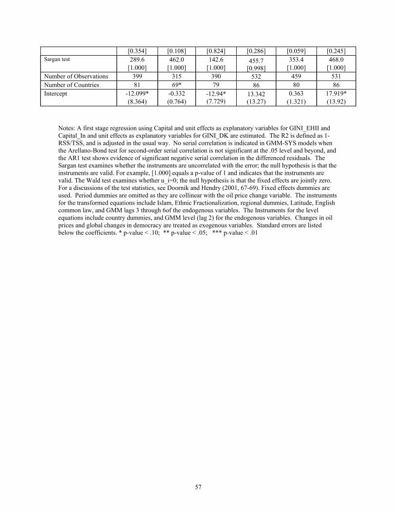
[0.354] [0.108] [0.824] [0.286] [0.059] [0.245] Sargan test 289.6 462.0 142.6 455.7

[0.998] 353.4

[1.000] 468.0

[1.000] [1.000] [1.000] [1.000] Number of Observations 399 315 390 532 459 531

81 69* Number of Countries 79 86 80 86 Intercept -12.099* -0.332 0.363

(0.764) -12.94* (7.729)

13.342 (13.27) (8.364) (1.321)

17.919* (13.92)

Notes: A first stage regression using Capital and unit effects as explanatory variables for GINI_EHII and Capital_In and unit effects as explanatory variables for GINI_DK are estimated. The R2 is defined as 1-RSS/TSS, and is adjusted in the usual way. No serial correlation is indicated in GMM-SYS models when the Arellano-Bond test for second-order serial correlation is not significant at the .05 level and beyond, and the AR1 test shows evidence of significant negative serial correlation in the differenced residuals. The Sargan test examines whether the instruments are uncorrelated with the error; the null hypothesis is that the instruments are valid. For example, [1.000] equals a p-value of 1 and indicates that the instruments are valid. The Wald test examines whether u_i=0; the null hypothesis is that the fixed effects are jointly zero. For a discussions of the test statistics, see Doornik and Hendry (2001, 67-69). Fixed effects dummies are used. Period dummies are omitted as they are collinear with the oil price change variable. The instruments for the transformed equations include Islam, Ethnic Fractionalization, regional dummies, Latitude, English common law, and GMM lags 3 through 6of the endogenous variables. The Instruments for the level equations include country dummies, and GMM level (lag 2) for the endogenous variables. Changes in oil prices and global changes in democracy are treated as exogenous variables. Standard errors are listed below the coefficients. * p-value < .10; ** p-value < .05; *** p-value < .01

57

Table 4a – The Determinants of Inequality Y=Change in Inequality, GMM-System

Variable Model 1 GINI_DK

Model 2 GINI_DK

Model 3 GINI_DK

Model 4 GINI_FQ3

∆GINI_DK (s-1) 0.313*** 0.305*** 0.198** (0.108) (0.110) (0.106)

∆GINI_FQ3 (s-1) 0.316*** (0.102)

∆CAPITAL (s-1) 0.022 (0.021)

0.034* (0.025)

∆CAPITAL_in (s-1) 0.105** (0.046)

-0.051 ∆CAPITAL_out (s-1) (0.048)

∆CAPITAL_in (s-1) emerging only

0.122** (0.054)

∆CAPITAL_out (s-1) emerging only

-0.044 (0.055)

∆Democracy 0.072 0.090 0.087 0.098 (0.113) (0.118) (0.129) (0.135)

∆Government Expenditures (s-1)

0.108* 0.097* 0.044 0.125* (0.070) (0.081) (0.068) (0.083)

∆Global Communist Party vote share (s-1)

-0.837** -1.041** -0.745 -0.872** (0.463) (0.444) (0.555) (0.630)

Member of EU (0,1) (s-1)

-0.942 8.300*** -0.677 (1.257) (1.459) (2.728)

-2.013 (1.924)

Member Soviet Bloc (0,1) (s-1)

-1.433 -0.394 -1.947 (2.124) (2.033) (1.973)

-1.991 (2.622)

∆Income (s-1) -3.216** -2.733** -1.798 (1.627) (1.546) (1.930)

-4.002** (1.782)

∆Growth (s-1) 0.222*** (0.090)

0.186** (0.094)

0.199** (0.087)

0.316*** (0.104)

∆Investment 0.262 (1.541)

0.515 (1.549)

-1.558 (1.748) (Share of GDP) (s-1)

-0.174 (1.655)

Population Growth (s-1)

-0.424 (0.455)

-0.561 -1.069* (0.473) (0.660)

-0.561 (0.614)

∆Oil Prices (s-1) 0.015 (0.015)

0.018 0.050*** 0.030** (0.016) (0.020) (0.018)

∆Trade Openness (s-1)

1.135 (1.607)

0.697 (1.514)

1.396 (1.605)

2.191 (1.951)

Adjusted R2 .81 .81 .80 .72

Wald (fixed effects) 157.8 177.6 213.5 [0.000]**

94.61

58

Table 4b – The Determinants of Inequality

[0.000]** [0.000]** [0.032]* AR1 -3.270 -3.317 -2.586

[0.010]** -3.723

[0.000]** [0.001]** [0.001]** AR2 -1.530 -1.796 -1.936

[0.053] -1.673 [0.094] [0.126] [0.072]

Sargan test 43.02 [1.000]

41.99 [1.000]

30.24 [1.000]

38.56 [1.000]

Number of Observations 329 328 219 329

Number of Countries 71 71 52 71 Intercept

Y=Change in Inequality, GMM-System

47.468*** (17.06)

44.660*** (16.61)

41.417** 49.518*** (20.86) (18.51)

Variable

Model 5 GINI_FQ3

Model 6 GINI_FQ3

Model 7 GINI_EHII

Model 8 GINI_EHII

∆GINI_DK (s-1) ∆GINI_FQ3 (s-1) 0.307*** 0.210** (0.100) (0.106)

∆GINI_EHII (s-1) 0.540*** 0.523*** (0.073) (0.073)

∆CAPITAL (s-1) 0.019** (0.010)

0.139*** 0.007 ∆CAPITAL_in (s-1) (0.057) (0.019) ∆CAPITAL_out (s-1) -0.050 0.022

(0.021) (0.062) 0.145**

(0.066) ∆CAPITAL_in (s-1)

emerging only

∆CAPITAL_out (s-1) emerging only

-0.045 (0.070)

0.123 0.125 -0.009 -0.008 ∆Democracy (0.142) (0.039) (0.152) (0.039) ∆Government Expenditures (s-1)

0.105* 0.026 0.0004 0.002 (0.082) (0.106) (0.033) (0.036)

∆Global Communist Party vote share (s-1)

-0.887 -0.784*** -0.954** (0.784) (0.217) (0.563)

-0.801*** (0.226)

Member of EU (0,1) (s-1)

-2.443* 6.730*** 1.740** (1.551) (1.605) (1.004)

1.730** (1.038)

Member Soviet Bloc (0,1) (s-1)

-0.784 -0.357 -3.373*** (2.495) (2.628) (0.889)

-2.511*** (0.750)

∆Income (s-1) -3.404** -2.313 -0.487 -0.694

59

(1.649) (2.113) (0.589) (0.621) ∆Growth (s-1) 0.272*** 0.284***

(0.107) 0.010

(0.068) -0.006

(0.111) (0.069) ∆Investment (Share of GDP) (s-1)

0.120 (1.676)

-2.182 (1.837)

-0.799 -1.001 (0.885) (0.860)

Population Growth (s-1)

-0.716 (0.638)

-1.272** -0.858** -0.832** (0.762) (0.449) (0.483)

∆Oil Prices (s-1) 0.034** (0.019)

0.070*** (0.022)

0.007 (0.009)

0.007 (0.009)

∆Trade Openness (s-1)

1.636 2.383 (1.931)

-0.654 (0.737)

-0.392 (1.845) (0.739)

Adjusted R2 .72 .79 .92 .92

Wald (fixed effects) 111.5 124.8 252.5 3518. [0.000]** [0.000]** [0.000]** [0.002]**

AR1 -3.763 [0.000]**

-2.995 [0.003]**

-3.932 -3.878 [0.000]** [0.000]**

AR2 -1.859 [0.063]

-1.626 [0.104]

0.4444 [0.657]

0.4356 [0.663]

Sargan test 34.70 [1.000]

23.87 [1.000]

20.39 [1.000]

18.33 [1.000]

Number of Observations 328 219 435 434

Number of Countries 52 78 78 71 Intercept 41.573** 32.742*** 45.697***

(17.71) (22.98) (7.740) 34.605***

(7.915) Notes: The R2 is defined as 1-RSS/TSS, and is adjusted in the usual way. No serial correlation is indicated in GMM-SYS models when the Arellano-Bond test for second-order serial correlation is not significant at the .05 level and beyond, and the AR1 test shows evidence of significant negative serial correlation in the differenced residuals. The Sargan test examines whether the instruments are uncorrelated with the error; the null hypothesis is that the instruments are valid. For example, [1.000] equals a p-value of 1 and indicates that the instruments are valid. The Wald test examines whether u_i=0; the null hypothesis is that the fixed effects are jointly zero. For a discussions of the test statistics, see Doornik and Hendry (2001, 67-69). Fixed effects dummies are used. Period dummies are omitted as they are collinear with the oil price change variable. The instruments for the transformed equations include Islam, Ethnic Fractionalization, regional dummies, Latitude, English common law, and GMM lags 3 through 6of the endogenous variables. The Instruments for the level equations include country dummies, and GMM level (lag 2) for the endogenous variables. Changes in oil prices and global changes in communist party vote shares are treated as exogenous variables. Standard errors are listed below the coefficients. * p-value < .10; ** p-value < .05; *** p-value < .01

60

Table 5 - Y=Change in Democracy, 1955-2004, GMM-System

The Pathway from Financial Globalization through Inequality to Democracy

Variable

Model 1 Model 2 Model 3 ∆Polity

Model 4 ∆Polity ∆Regime ∆Regime

Polity or Regime (s-1) -0.315*** -0.234*** (0.048)

-0.300*** (0.085) (0.078)

-0.333*** (0.110)

Polity or Regime (s-2) -0.243*** -0.321*** (0.081)

-0.226*** (0.078)

-0.352*** (0.071) (0.099)

∆World Democracy 0.002 (0.004)

0.060 0.002 (0.006)

0.019 (0.048) (0.098)

-0.048*** (0.017)

-0.004*** ∆CAPITAL (s-1) (0.001) ∆CAPITAL_in (s-1) -0.029 -0.001

(0.025) (0.002) -0.001

(0.023) 0.002 ∆CAPITAL_out (s-1) (0.002)

Predicted value of ∆GINI_DK (s-1) from Capital_In

-0.499* -0.045** (0.264) (0.022)

Predicted Value of ∆GINI_DK sq (s-1) from Capital_In

0.008** 0.001** (0.003) (0.000)

Predicted value of ∆GINI_EHII (s-1) from Capital

-5.093*** -0.295* (1.589) (0.167)

Predicted Value of ∆GINI_EHII sq (s-1) from Capital

0.072*** 0.004* (0.002) (0.023)

Regional Democracy (s-1) 0.334** (0.145)

0.007 (0.009)

0.244* 0.023** (0.138) (0.011)

Member of EU (0,1) (s-1) -1.802 (1.137)

-0.185** (0.091)

0.679 0.082 (0.867) (0.109)

Member Soviet Bloc (0,1) (s-1)

6.443*** (1.892)

0.620*** (0.184)

2.054 (1.768)

0.386*** (0.133)

∆Income (s-1) 0.463 0.056 (0.072)

1.397 (0.880)

0.160** (1.002) (0.069)

∆Growth (s-1) 0.016 0.005 (0.080) (0.006)

-0.195** (0.089)

-0.006 (0.007)

∆Investment -0.012 (0.775)

-0.035 (0.054)

-0.261 0.018 (0.720) (Share of GDP) (s-1) (0.104)

Population Growth (s-1)

-0.745* (0.387)

-0.010 (0.018)

-0.023 -0.013 (0.2113) (0.023)

∆Oil Prices (s-1) -0.024* (0.013)

-0.002* (0.001)

-0.029 (0.040)

-0.001 (0.003)

∆Trade Openness (s-1) 0.650 0.068 0.810 -0.017

61

Notes: A first stage regression using Capital and unit effects as explanatory variables for GINI_EHII and Capital_In and unit effects as explanatory variables for GINI_DK are estimated. The predicted values of

(1.112) (0.084) (0.639) (0.052) Adjusted R2 0.327 0.368 0.268 0.307

1827 203.7 22580 Wald (fixed effects) 8820 χ-square distribution [0.000] [0.000] [0.000] [0.000]

-2.703** -2.681** -3.602** -4.070** AR1 [0.007] [0.007] [0.000] [0.000] 0.1207 [0.904]

-1.546 [0.122]

1.057 [0.290]

0.3801 AR2 [0.704]

Sargan test 518.8 [1.000]

449.5 [1.000]

187.9 [1.000]

410.6 [0.990]

Number of Observations 390 311 521 425 Number of Countries 77 69 85 80

1.931 Intercept 0.181 73.381*** (2.52) (0.180) (25.43)

3.871 (2.602)

GINI are substituted for the observed values, and the models from Table 3 are reestimated in Table 5. The R2 is defined as 1-RSS/TSS, and is adjusted in the usual way. No serial correlation is indicated in GMM-SYS models when the Arellano-Bond test for second-order serial correlation is not significant at the .05 level and beyond, and the AR1 test shows evidence of significant negative serial correlation in the differenced residuals. The Sargan test examines whether the instruments are uncorrelated with the error; the null hypothesis is that the instruments are valid. For example, [1.000] equals a p-value of 1 and indicates that the instruments are valid. The Wald test examines whether u_i=0; the null hypothesis is that the fixed effects are jointly zero. For a discussions of the test statistics, see Doornik and Hendry (2001, 67-69). Fixed effects dummies are used. Period dummies are omitted as they are collinear with the oil price change variable. The instruments for the transformed equations include Islam, Ethnic Fractionalization, regional dummies, Latitude, English common law, and GMM lags 3 through 6of the endogenous variables. The Instruments for the level equations include country dummies, and GMM level (lag 2) for the endogenous variables. Changes in oil prices and global changes in democracy are treated as exogenous variables. Standard errors are listed below the coefficients. * p-value < .10; ** p-value < .05; *** p-value < .01

62

Appendix Table A1

Giniall giniadjustDK giniadjustFQ3 EHII Giniall 1 giniadjustDK 0.97886252 1 giniadjustFQ3 0.93311012 0.98650937 1 EHII 0.6294634 0.6087542 0.59235781 1

Notes: Gini_all is the unadjusted WIID 2008 data; Gini_adjust_DK is the WIID data adjusted using the algorithm in Dollar and Kraay 2002; Gini_adjust_FQ3 is the WIID data adjusted using the results of a regression estimated with dummy variables for dummy variables for consumption vs income, gross vs. net income, and household vs. individual surveys. EHII is the indicator from Galbraith and Kum 2005.

Appendix Table A2

EHII giniall5 giniallDK5 giniallFQ52 giniallFQ53 SIDD EU -0.30309 -0.29018 -0.21651 -0.15921 -0.1249 -0.18558 islam2 0.320977 -0.00828 -0.03831 -0.04 -0.05315 ETHFRAC 0.519283 0.405105 0.364185 0.335578 0.30023 SSA 0.350795 0.217032 0.203596 0.201444 0.18263 0.318472 EAP 0.000657 -0.01054 -0.06085 -0.09998 -0.09727 -0.03451 EUROPE -0.47712 -0.35585 -0.27314 -0.20925 -0.15819 -0.29338 SASIA 0.151731 -0.13774 -0.15768 -0.16001 -0.15782 -0.11105 MENA 0.142483 0.024686 0.032712 0.051285 0.045956 0.114516 LAC 0.300085 0.595267 0.572399 0.533584 0.493043 0.518573 ENGLISH 0.140851 0.001929 -0.03217 -0.05338 -0.04079 0.014456 LATITUDE -0.49232 -0.58817 -0.53244 -0.48216 -0.44229 -0.55859 FRENCH 0.334958 0.418734 0.424959 0.424013 0.400958 0.469111 SOCIAL -0.41 -0.3986 -0.39545 -0.38952 -0.40257 -0.51104 GERMAN -0.19226 -0.18793 -0.17664 -0.16963 -0.15423 -0.18126 OECD -0.56166 -0.413 -0.35103 -0.30494 -0.24784 -0.36156 soviet -0.37937 -0.33258 -0.33912 -0.34113 -0.3545 -0.42563

Notes: See notes for Appendix Table A1. The correlates are regional dummies from the World Bank or indicators of a country’s legal origin, or measures of its ethnic fractionalization, Islamic population percentages, or its latitude.

63

Table A3 – Dependent Variable = REGIME, 1960-2004, GMM-System Estimations 0=Autocracy, 1=Democracy; Instruments= Income (s-2); Currency Crises (s-1);

Global Average of Capital Account Openness (s-1) Variable

1

Full Sample

RE

2 3 Emerging Markets

RE

4 Emerging Markets

Full Sample

FE FE CAPITAL (s-1) 0.029***

(0.008) -0.005* (0.003)

0.012 (0.008)

-0.008** (0.003)

Prior Transitions to Dictatorship(s-1)

0.003** (0.001)

0.113 (0.126)

0.005** (0.002)

0.078 (0.091)

Log(Constitutional Age(s-1))

0.014 (0.010)

0.062*** (0.018)

0.007 (0.011) 0.004 (0.015)

World Democracy (s-1) -0.014 (0.011)

0.015*** (0.004)

0.002 (0.015)

0.025*** (0.006)

Natural Resource Export -0.017** (0.007)

-0.070*** (0.009)

-0.018* (0.010)

-0.084*** (0.021)

Socialist Legal Origin -0.002* (0.001)

-0.302*** (0.077)

-0.002 (0.002)

-0.014 (0.047)

Latin America -0.009** (0.003)

0.044** (0.022)

0.040* (0.021)

0.413*** (0.032)

Middle East and North Africa

-0.005** (0.002)

-0.702*** (0.089)

0.007** (0.003)

-0.208*** (0.036)

Sub-Saharan Africa -0.019** (0.008)

-0.340*** (0.005)

-0.048* (0.026)

0.009 (0.049)

Asia -0.018** (0.007)

-0.011 (0.019)

-0.030* (0.016)

0.146*** (0.019)

British Colonial Heritage -0.011** (0.005)

0.058*** 0.007

-0.030* (0.017)

0.166*** (0.010)

French Colonial Heritage -0.006* (0.003)

-0.058*** (0.022)

-0.0002 (0.002)

-0.005 (0.016)

Spanish Colonial Heritage -0.009** (0.004)

-0.009 (0.004)

0.028* (0.015)

0.167** (0.074)

Log(GDP Per Capita PPP(s-1))

-0.077* (0.040)

0.060 (0.062)

0.018 0.003 (0.031) (0.071)

Growth (s-1) -0.088 (0.054)

-0.023 (0.019)

-0.163** (0.073)

-0.012 (0.032) 0.172

Urban Population -0.033* (0.017)

0.217 (0.150)

0.042 (0.015) (0.136)

Population Density (s-1) 0.003 (0.002)

-0.118*** (0.015)

0.027 (0.013)

-0.014** (0.019)

Fixed Effects? No Yes No Yes Wald Test (Fixed Effects) χ-square distribution

163.00*** (0.00)

44.55

Countries/Observations 82/582 82/582 60/409 60/409 Number of Observations 582 582 409 409

Intercept -0.023** (0.010)

-0.507*** (0.064)

-0.032* (0.019)

-0.226* (0.119)

64

Table A4 - Dependent Variable = Change in POLITY, 1960-2004, GMM-System Estimations; Instruments= Income (s-2); Currency Crises (s-1); Global

Average of Capital Account Openness (s-1) Variable

1

Full Sample

RE

2 Full

Sample FE

3 Emerging Markets

RE

4 Emerging Markets

FE CAPITAL (s-1) -0.033***

(0.011)

-0.048*

(0.029) -0.117***

(0.035) -0.090** (0.037)

Democracy (s-1) -0.018

(0.035) 0.185

(0.134) 0.002

(0.024) -0.013 (0.032)

Prior Transitions to Dictatorship(s-1)

0.007*** (0.002)

3.389** (1.383)

0.007*** (0.002)

3.442*** (1.006)

Log(Constitutional Age(s-1))

0.142*** (0.036)

-0.151 (0.148)

0.259*** (0.067)

0.265 (0.172)

World Democracy (s-1) -0.043 (0.039)

-0.040 (0.039)

-0.019 (0.072)

0.005 (0.051)

Natural Resource Export 0.022*** (0.006)

-0.378*** (0.054)

0.025*** (0.007)

0.275 (0.261)

Socialist Legal Origin 0.008*** (0.002)

0.387 (0.683)

0.008*** (0.002)

-0.123 (0.483)

Latin America -0.005*** (0.002)

-0.005 (0.002)

0.004 (0.008)

-0.255 (0.219)

Middle East and North Africa

0.006*** (0.002)

-1.226** (0.588)

0.008*** (0.003)

-1.663*** (0.323)

Sub-Saharan Africa 0.045*** (0.011)

-0.409** (0.191)

0.035*** (0.012)

-0.215 (0.471)

Asia 0.009*** (0.002)

0.077 (0.167)

0.005 (0.005)

0.240 (0.209)

British Colonial Heritage 0.024*** (0.006)

0.024*** (0.006)

0.031*** (0.009)

-0.527*** (0.115)

French Colonial Heritage 0.035*** (0.009)

0.035* (0.009)

0.036*** (0.009)

-0.496*** (0.175)

Spanish Colonial Heritage -0.018*** (0.005)

-0.018 (0.005)

-0.012** (0.006)

1.245* (0.713)

Log(GDP Per Capita PPP(s-1))

0.341*** (0.085)

-0.221 (0.665)

0.646*** (0.168)

-0.726 (0.717)

Growth (s-1) -0.681*** (0.175)

-0.622*** (0.135)

-0.299*** (0.084)

-0.421* (0.254)

Urban Population 0.149*** (0.037)

1.859 (1.558)

0.315*** (0.083)

2.994** (1.448)

Population Density (s-1) 0.031*** (0.008)

0.545*** (0.181)

0.039*** (0.012)

0.725*** (0.196)

Fixed Effects? No Yes No Yes Wald Test (Fixed Effects)

χ-square distribution 1310.0***

(0.000) 967.4***

(0.000) Emerging Only? No No Yes Yes

Number of Countries 82/582 82/582 60/409 60/409 Intercept 0.149

(0.876) 0.028*** (0.007)

0.062*** (0.016)

0.210 (1.166)

65

Table A5 – Determinants of Corporate Tax Rates Dependent Variable = Top Corporate Tax Rate.

Variable

Model 1 Model 2 Model 3 Model 4 GMM_System Estimation

GMM_System Estimation

OLS with PCSE

OLS with PCSE

Full Sample Emerging Only Full SampleEmerging Only

Capital Tax Rates (s-1) 1.074*** 0.979*** 0.902*** 0.741*** (0.096) (0.120) (0.01) (0.157)

Home Capital Tax Rates minus U.S. Capital Tax Rates (s-1)

-0.493*** -0.443*** -0.412*** (0.077) (0.093) (0.078)

-0.334*** (0.106)

∆CAPITAL (s-1) 0.040* 0.054* 0.048** (0.021) (0.030) (0.019)

0.078*** (0.023)

Global Capital Account Openness (s-1

0.036 0.0286 -0.042 (0.048) (0.010) (0.054)

-0.186* (0.105)

∆Economic Growth (s-1)

-0.035 0.111 -0.134 (0.168) (0.094) (0.103)

0.024 (0.111)

∆Member of EU (0,1) 2.224 (1.424)

2.715 (1.693)

∆Income (s-1) 1.791 (1.407)

1.078 (2.117)

0.912 (1.136)

1.310 (1.414)

∆Investment (s-1) (Share of GDP)

-0.876 (1.288)

-0.119 -0.879 (1.316) (1.372)

-1.161 (1.439)

∆Government Share of GDP (s-1)

0.091 (0.075)

0.058 (0.090)

0.138** (0.066)

-0.048 (0.09)

∆Population Growth (s-1)

-0.744 (0.720)

0.680 1.012* (0.550)

0.565 (0.672) (1.473)

∆Democracy (s-1) 1.791 -0.077 (0.112)

0.138 (0.088)

-0.037 (0.105) (1.407)

∆Trade Openness(s-1) -0.087 -1.328 (1.655)

0.694 (1.298)

2.330 (1.812) (1.587)

∆Revolutions & Coups (s-1) -0.093 (0.289)

-0.004 (0.362)

-0.093 (0.222)

-0.110 (0.264)

Wald 430.1 [0.000]**

330.9 [0.000]**

Sargan 0.999 1.000 AR1 -4.076

[0.000]** -3.133

[0.002]**

AR2 -1.218 [0.223]

-1.696 [0.090]

Durbin’s M -0.031 -0.046 (0.051) (0.066)

Number of Obs 444 276 417 249 Countries 82 60 78 56 Constant -18.205

(12.230) -9.442

(16.770) -12.194 (14.010)

-7.938 (16.360)

66

Appendix Table 6 - Y=Change in Democracy, 1955-2004, GMM-System Channels from Financial Globalization to Inequality to Democracy

Capital or Capital_In Omitted Variable

Model 5 Model 6 Model 7 Model 8 ∆Regime ∆Polity ∆Regime ∆Polity

Polity or Regime (s-1) -0.360*** (0.092)

-0.319*** -0.235*** -0.359*** (0.115) (0.076) (0.051)

Polity or Regime (s-2) -0.167** (0.071)

-0.189*** -0.326*** -0.324*** (0.095) (0.063) (0.079)

∆World Democracy 0.005 (0.050)

0.053 0.002 0.001 (0.097) (0.004) (0.006)

∆CAPITAL (s-1) ∆CAPITAL_in (s-1)

-0.009 0.002 ∆CAPITAL_out (s-1) (0.026) (0.002)

Predicted value of ∆GINI_DK (s-1) from Capital_In

-38.199* -2.027 (20.20) (1.263)

0.370 0.022 (0.015)

Predicted Value of ∆GINI_DK sq (s-1) from Capital_In

(0.235)

-6.403*** Predicted value of ∆GINI_EHII (s-1) from Capital

(1.905) -0.414** (0.181)

Predicted Value of ∆GINI_EHII sq (s-1) from Capital

0.072*** 0.005** (0.002) (0.023)

Regional Democracy (s-1) 0.336** (0.148)

0.245* 0.008 (0.010)

0.021* (0.011) (0.138)

Member of EU (0,1) (s-1) 0.786 -0.167* (0.100)

0.093 (0.109)

-0.851 (0.844) (1.322)

Member Soviet Bloc (0,1) (s-1)

1.866 (1.845)

0.605*** (0.184)

0.330** 5.750*** (1.959) (0.141)

∆Income (s-1) 0.767 1.774** (0.889)

0.070 (0.075)

0.195** (1.079) (0.075)

∆Growth (s-1) 0.034 -0.203** 0.004 (0.006)

-0.006 (0.008) (0.085) (0.092)

∆Investment (Share of GDP) (s-1)

-0.165 (0.935)

-0.244 (0.673)

-0.037 (0.057)

0.024 (0.093)

Population Growth (s-1) -0.720* (0.407)

0.005 (0.217)

-0.009 -0.010 (0.018) (0.024) ∆Oil Prices (s-1) -0.026* -0.029 -0.002* -0.001

(0.013) (0.039) (0.001) (0.003) ∆Trade Openness (s-1) 0.977 0.437 0.074 -0.032

(1.238) (0.599) (0.085) (0.054) Adjusted R2 0.268 0.375 0.308 0.340

4.126e+9 137.7 4.468e+10 Wald (fixed effects) 192.8 [0.000] [0.000] [0.000] [0.000]

-2.657 -3.590 -2.673 AR1 -3.865

67

[0.008] [0.000] [0.008] [0.000] -0.347 0.670 -1.576 0.294 AR2 [0.729] [0.503] [0.115] [0.769]

289.9 238.9 397.0 Sargan test 147.8 [1.000] [1.000] [0.926] [1.000]

Number of Observations 521 311 452 382 Number of Countries 85 69 80 77 Intercept

Notes: A first stage regression using Capital and unit effects as explanatory variables for GINI_EHII and Capital_In and unit effects as explanatory variables for GINI_DK are estimated. The predicted values of GINI are substituted for the observed values, and the models from Table 3 are reestimated in Table 5. The R2 is defined as 1-RSS/TSS, and is adjusted in the usual way. No serial correlation is indicated in GMM-SYS models when the Arellano-Bond test for second-order serial correlation is not significant at the .05 level and beyond, and the AR1 test shows evidence of significant negative serial correlation in the differenced residuals. The Sargan test examines whether the instruments are uncorrelated with the error; the null hypothesis is that the instruments are valid. For example, [1.000] equals a p-value of 1 and indicates that the instruments are valid. The Wald test examines whether u_i=0; the null hypothesis is that the fixed effects are jointly zero. For a discussions of the test statistics, see Doornik and Hendry (2001, 67-69). Fixed effects dummies are used. Period dummies are omitted as they are collinear with the oil price change variable. The instruments for the transformed equations include Islam, Ethnic Fractionalization, regional dummies, Latitude, English common law, and GMM lags 3 through 6of the endogenous variables. The Instruments for the level equations include country dummies, and GMM level (lag 2) for the endogenous variables. Changes in oil prices and global changes in democracy are treated as exogenous variables. Standard errors are listed below the coefficients. * p-value < .10; ** p-value < .05; *** p-value < .01

68

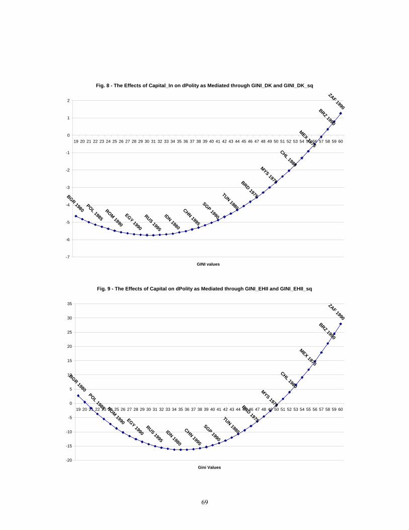
Fig. 8 - The Effects of Capital_In on dPolity as Mediated through GINI_DK and GINI_DK_sqZAF 1990BRZ 1990

MEX 1975CHL 1980

MYS 1975BRD 1975TUN 1980SGP 1990

CHN 1995IDN 1980

RUS 1995

EGY 1990

ROM 1990

POL 1985

BGR 1980

-7

-6

-5

-4

-3

-2

-1

0

1

2

19 20 21 22 23 24 25 26 27 28 29 30 31 32 33 34 35 36 37 38 39 40 41 42 43 44 45 46 47 48 49 50 51 52 53 54 55 56 57 58 59 60

GINI values

Fig. 9 - The Effects of Capital on dPolity as Mediated through GINI_EHII and GINI_EHII_sq

ZAF 1990BRZ 1990

MEX 1975

CHL 1980MYS 1975BRD 1975TUN 1980

SGP 1990

CHN 1995

IDN 1980

RUS 1995

EGY 1990

ROM 1990

POL 1985

BGR 1980

-20

-15

-10

-5

0

5

10

15

20

25

30

35

19 20 21 22 23 24 25 26 27 28 29 30 31 32 33 34 35 36 37 38 39 40 41 42 43 44 45 46 47 48 49 50 51 52 53 54 55 56 57 58 59 60

Gini Values

69

Fig. 10 - The Effect of Capital_In on dRegime as Mediated by GINI_DK & GINI_DK_sq

ZAF 1990BRZ 1990MEX 1975CHL 1980MYS 1975BRD 1975

TUN 1980SGP 1990

CHN 1995

IDN 1980

RUS 1995

EGY 1990

ROM 1990

POL 1985

BGR 1980

-0.7

-0.6

-0.5

-0.4

-0.3

-0.2

-0.1

019 20 21 22 23 24 25 26 27 28 29 30 31 32 33 34 35 36 37 38 39 40 41 42 43 44 45 46 47 48 49 50 51 52 53 54 55 56 57 58 59 60

Gini Values

Fig. 11 - The Effect of Capital on dRegime as Mediated by GINI_EHII & GINI_EHII_sq

ZAF 1990

BRZ 1990

MEX 1975

CHL 1980

MYS 1975BRD 1975TUN 1980

SGP 1990

CHN 1995

IDN 1980

RUS 1995

EGY 1990

ROM 1990

POL 1985

BGR 1980

-1.5

-1

-0.5

0

0.5

1

1.5

2

19 20 21 22 23 24 25 26 27 28 29 30 31 32 33 34 35 36 37 38 39 40 41 42 43 44 45 46 47 48 49 50 51 52 53 54 55 56 57 58 59 60

GINI values

70