1

Summarizing Data using Bottom-k Sketches

Edith Cohen AT&THaim Kaplan Tel Aviv University

2

The basic application setupThere is a universe of items, each has a weight

Keep a sketch of k items, so that you can estimate the weight of any subpopulation from the sketch. (also other aggregates, weight functions)

Example:

Items are flows going through a router w(i) is the number of packets of flow i . Queries supported by the sketch are estimates on the total weight of flows of a particular port, particular size, particular destination IP address, etc.

w(i1)

w(i2)

w(i3)

3

Application setup: Coordinated sketches for multiple

subsetsUniverse I of weighted items and a set of subsets over that universe.

Keep a size-k sketch of each subset, so that you can support both queries within a subset and queries on subset relations such as aggregates over union, or intersection, resemblance….These sketches are coordinated so that subset relations queries can be supported better.

4

…Sketches for multiple subsets

Example applications:

•Items are features and subsets are documents. Estimate similarity of documents.

•Items are documents and subsets are features. Estimate “correlation” of features.

•Items are files and subsets are neighborhoods in a p2p network. Estimate total size of distinct items in a neighborhood.

•Items are goods and subsets are consumers. Estimate marketing cost of all goods in a subset of consumers.

5

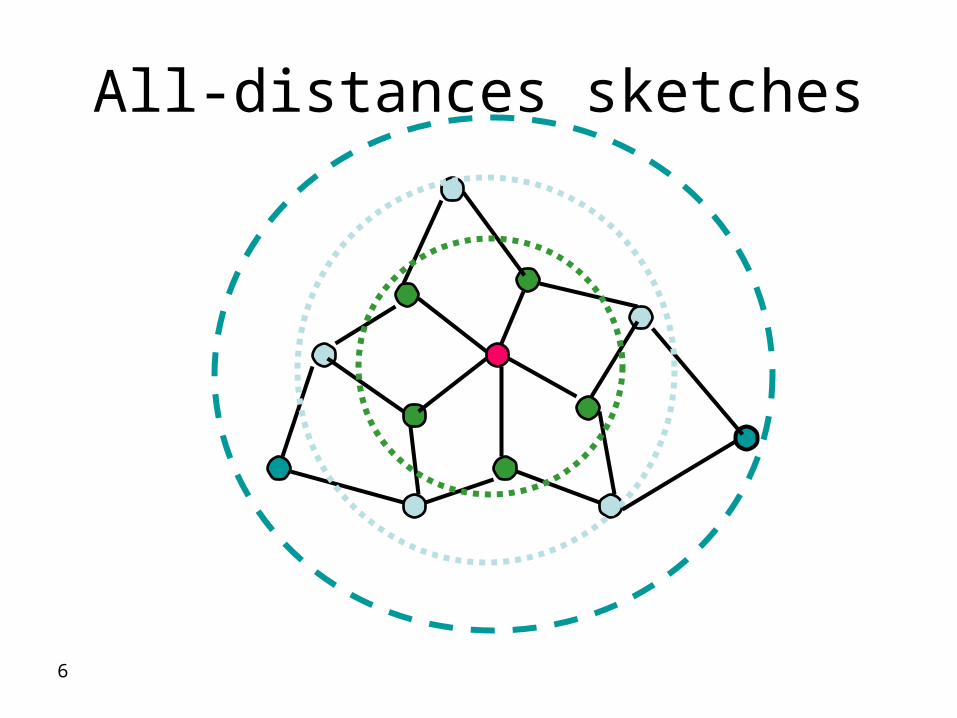
Application setup: All-distances sketches

Items are located in a metric space (data stream with time stamp or sequence number, network with distance).

All-distances sketch of a location v is a compact encoding of the sketches of ALL neighborhoods of v.

Efficient time-decaying and spatially-decaying aggregation

For each query distance d, the sketch of the set of items within distance d from v can be retrieved from the all-distances sketch v

6

All-distances sketches

7

One approach: k-mins sketches

•Each item i draws a rank r(i) from an exponential distribution with parameter w(i) (-ln u/w(i) u [0,1]∊ )

•Pick the item with the smallest rank to your set

•Repeat k times (possibly concurrently)

Equivalent to weighted sampling of k items with replacement, (convenient in distributed settings).

k-mins sketch (Cohen 97)

( (i2,r (1)(i2), (i2,r (k)(i2) )(i5,r (2)(i5) ,….

8

…… k-mins sketchesMultiple subsets: same r(1) ,…,r(k) for all subsets.

All-distances: encode min rank at any distance (0,0.8), (2,0.6), (10,0.5), (15,0.2)Estimators (examples):

•The fraction of blue items among the k in the sketch is an unbiased estimate of their fraction in the population

• (k-1)/sum(k min ranks) is an unbiased estimate of the weight of the set (error decreases with k)

•Multiple subsets: fraction of “common” coordinates is an unbiased estimator for resemblance (ratio of intersection and union)

x k

9

Applications of k-mins sketchesGraph theory: Estimate the size of the transitive closure of a directed graph and of neighborhoods without explicitly computing them (Cohen ’94)

Sensor networks: Estimating # of items, variance, in a neighborhood of a sensor (Cohen, Kaplan, SIGMOD’04), aggregation where weights decay with distance

Streaming: aggregation where weights decay with time (Cohen, Strauss, PODS’03)

Databases: Estimate the size of the “join” before actually computing it (Lewis, Cohen SODA’97)

Data mining: Estimate resemblance of Web pages and Web sites (Broder 97, Bharat, Broder 99,…)

Databases: Estimate association rules (CDFGM TKDE ’01)

10

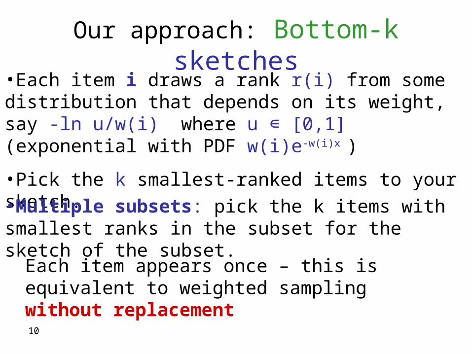
Our approach: Bottom-k sketches

Each item appears once – this is equivalent to weighted sampling without replacement

•Each item i draws a rank r(i) from some distribution that depends on its weight, say -ln u/w(i) where u [0,1]∊ (exponential with PDF w(i)e-

w(i)x )

•Pick the k smallest-ranked items to your sketch.•Multiple subsets: pick the k items with smallest ranks in the subset for the sketch of the subset.

11

Advantages of Bottom-k sketches

Intuitively the sample is more informative, in particular for Zipf-like distribution, where there are few large weights.

Often, more efficient to compute

Provide more accurate estimates

Bottom-k sketches can be used instead of k-mins sketches in almost every application

12

Bottom-k sketches can replace k-mins sketches in most

applications•Plain sketches for explicitly-represented subsets: Bottom-k sketches can be computed much more efficiently.

•All-distance sketches: Bottom-k sketches can be computed as efficiently

? Open: Euclidean plane

13

Multiple subsets with explicit representation

Items are processed one by one, sketch is updated when a new item is processed:

k-mins: The new item draws a vector of k random numbers

We compare each coordinate to the “winner” so far in that coordinate and update if the new one wins

O(k) time to test and updatebottom-k: The new item draws one random number

We compare the number to the k smallest so far and update if smaller

O(1) time to test O(log k) time to update

14

…Multiple subsets with explicit representation

The number of tests = sum of the sizes of subsets.

The number of updates is “generally” logarithmic (depends on item-weights distribution and the order items are processed) and about the same for k-mins and bottom-k sketches. (Precise analysis in the paper)

k-mins: O(k) time to test and update

bottom-k: O(1) time to test O(log k) time to update

15

All distances bottom-k sketches

Data structures are more complex than all-distances k-mins sketches -- maintain k smallest items in a single rank assignment instead of one smallest in k independent assignments.

We analyze the number of operations for

•Constructing all-distances k-mins and bottom-k sketches for different orders in which items are “processed”, weight distributions, and relations of weight and location.

•Querying sketches

The number of operations is comparable for both types of sketches.

16

Bottom-k sketches provide more accurate estimates

The red line shows an estimate based on k-mins sketch

All other lines are various estimators that use bottom-k sketch

17

Estimating with bottom-k sketches (by “mimicking”)

We can produce from a bottom-k sketch S a distribution D(S) on k-mins sketches.

Drawing S and then a k-mins sketch from D(S) is equivalent to drawing a k-mins sketchCan use all known estimators for k-mins sketch

We can do even better by taking expectation over D(S) or drawing from D(S) multiple times

bottom-k

sketches S

k-mins sketchesD(S)

18

Maximum likelihood estimate using bottom-k sketches

Lemma: Over sketches with item weights (w1,w2,…wk) The rank differences are independent, each distributed exponentially

r1 – r0 r2 – r1

...

rk-rk-1

exp. with parameter W= w(I)exp. with parameter W-w1

exp. with parameter W-w1-w2-...-wk-1

The probability that we see the particular differences is

1

111 1 2 1

1 ( )( )( )( )

11

( ) ( ) .....( )

k

i k ki

k W w r rWr W w r r

ii

We W w e W w e

The ML estimate is the W which maximizes this

19

Adjusted weights estimatorsOld technique by Horvitz and Thompson:

Let pi be the probability that item i is sampled.

Assign to item i an adjusted weight of a(i)=w(i)/pi if i is sampled and a(i)=0 otherwise. Then

a(i) is an unbiased estimator of w(i)

To estimate a subset J we sum up the adjusted weights of the elements of the sketch that are in J

)(0)1()(

))(( iwpp

iwpiaE i

ii

20

Subspace conditioningProblem: pi may be impossible or hard to compute from the information in the sketch.

Partition the probability space into subspaces and apply the technique within each subset.pi is now the probability that wi is in the sketch conditioned on the fact that the sketch is from a particular subspace.

Our idea:

21

Rank conditioning estimatorsPartition the sketches according to the (k+1)-smallest rank (rk+1) (kth smallest rank among all other items)Then pi is the probability that the rank of i is smaller than rk+1

Lemma: E(a(i)a(j)) = w(i)w(j) (cov(i,j)=0) i<>j

the variance of the estimator for a subset J is the sum of the variances of the adjusted weights of the items in J

1)(1 kriwi ep

22

Reducing the variance

Use a coarser partition of the probability space to do the conditioning

Lemma: The variance is smaller for a coarser partition.

Typically pi gets somewhat harder to compute

23

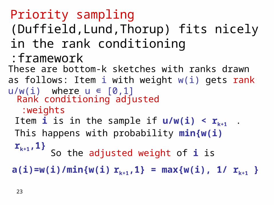
Priority sampling (Duffield,Lund,Thorup) fits nicely in the rank conditioning framework:

These are bottom-k sketches with ranks drawn as follows: Item i with weight w(i) gets rank u/w(i) where u ∊ [0,1]

Item i is in the sample if u/w(i) < rk+1 . This happens with probability min{w(i) rk+1,1}

So the adjusted weight of i is

a(i)=w(i)/min{w(i) rk+1,1} = max{w(i), 1/ rk+1 }

Rank conditioning adjusted weights:

24

Other weight functions

• We can estimate aggregates with respect to other weight functions, such as, number of distinct items, size distribution….

• For a numeric property h(i), h(i)a(i)/w(i) is an unbiased estimator of h(i). Therefore,

sJiJi iw

iaih

iw

iaih

)(

)()(

)(

)()(

is an unbiased estimator of h(J)

25

Other aggregates

• Selectivity of a subpopulation• Approximate quantiles• Variance and higher moments• Weighted random sample• ……

26

Summary: bottom-k sketches • Useful in many application setups:

– Sketch a single set– Coordinated sketches of multiple subsets– All-distances sketches

• A better alternative to k-mins sketches• We facilitate use of bottom-k sketches:

– Data structures, all-distances sketches– Analyze construction and query cost– Estimators, variance, confidence intervals

[also in further work]