1

Software Fault Tolerance (SWFT)Software Testing

Dependable Embedded Systems & SW Group www.deeds.informatik.tu-darmstadt.de

Prof. Neeraj Suri

Constantin Sârbu

Dept. of Computer ScienceTU Darmstadt, Germany

2

Fault Removal: Software Testing So far: checkpointing, recovery blocks, NVP, NCP, microreboots …

Verification & Validation Testing Techniques Static vs. Dynamic Black-box vs. White-box

Today: Testing of dependable systems Modeling Fault-injection (FI / SWIFI) Some existing tools for fault injection

Next 2 lectures: Testing of operating systems Fault injection aspects in OSs (WHEN / WHAT to inject) Profiling the OS extensions (state change @ runtime)

3

Why is PERFECT testing impossible? HW/OS/SW/Protocols our fault/error models are speculative failure modes and associated failure distributions are

probabilistic sequences (# of data cascades, # temporal links) do

not follow any meaningful distributions state space: fault classes only condense equivalent

behavior states – nothing more lack of details available! [processor level, gate,

device, transistor, VHDL?] fixing bugs often causes more bugs (bug re-injections) cause of bugs is more important: complex spec?

complex dependency?

How good are our system models?

4

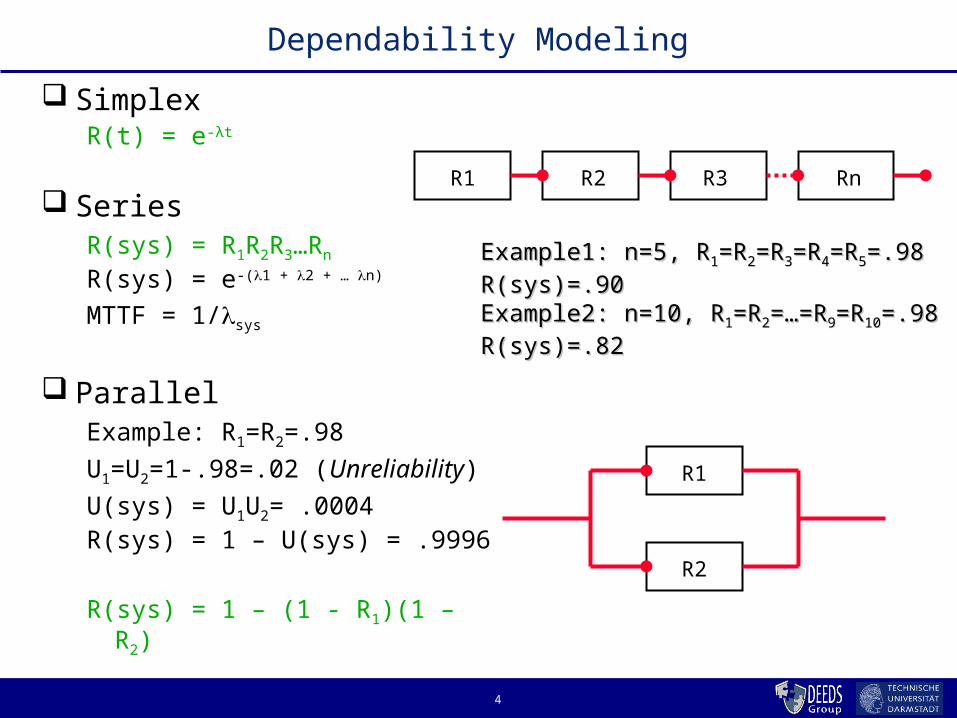
Dependability Modeling

SimplexR(t) = e-λt

Series R(sys) = R1R2R3…Rn R(sys) = e-(1 + 2 + … n)

MTTF = 1/sys

ParallelExample: R1=R2=.98

U1=U2=1-.98=.02 (Unreliability)

U(sys) = U1U2= .0004R(sys) = 1 – U(sys) = .9996

R(sys) = 1 – (1 - R1)(1 – R2)

R1 R2 R3 Rn

R1

R2

Example1: n=5, RExample1: n=5, R11=R=R22=R=R33=R=R44=R=R55=.98=.98R(sys)=.90R(sys)=.90Example2: n=10, RExample2: n=10, R11=R=R22=…=R=…=R99=R=R1010=.98=.98R(sys)=.82R(sys)=.82

5

Dependability Modeling

TMR: is this a parallel system? Works as long as two units

are fault-free Assumes independent faults Perfect voter No repair!

Reliability:

Where did this come from?

P1

P2

P3

= o/p tt eetR 32 23)(

6

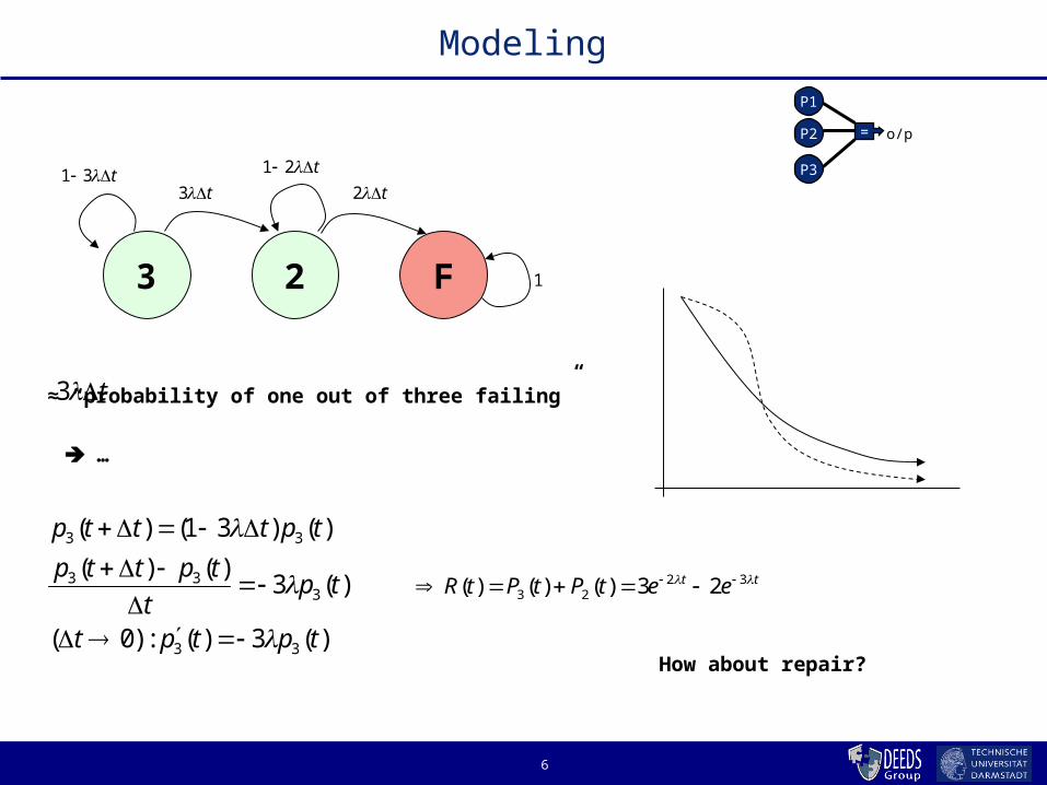
Modeling

P1

P2

P3

= o/p

2 F3

t3

t 21

t2

1

t3 ≈ “probability of one out of three failing”

…

)(3)(:)0(

)(3)()(

)()31()(

33

333

33

tptpt

tpt

tpttp

tptttp

tt eetPtPtR 3223 23)()()(

t 31

How about repair?

7

Modeling (Markov)

2 F3

t3

t 21

t2

1

t 31

t

Solving this system gives:

P1

P2

P3

= o/p

λ1

MTTF ntnonredunda =Do we always have perfect detection?

Can the system go directly from 3 to F?

2repair/w λ6μ

λ65

MTTF +=

but

λ65

MTTFrepairo/w

=

= 1000 h

= 833 h

= 17500 h

for λ = 0.001; µ =0.1

8

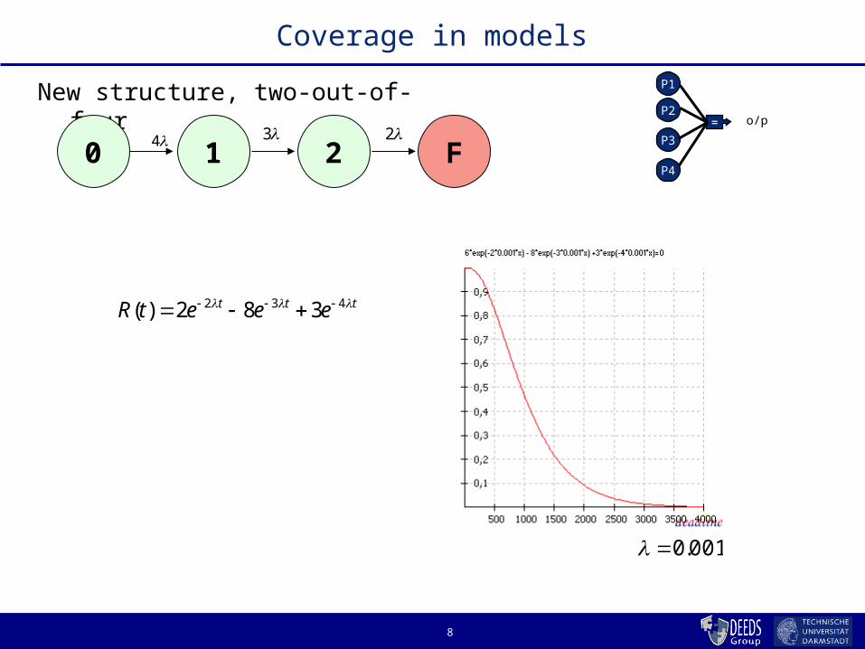
Coverage in models

New structure, two-out-of-four

2 F104 3 2

P1

P2

P3

= o/p

P4

ttt eeetR 432 382)(

001.0

9

Coverage in models

New structure, two-out-of-four P1

P2

P3

= o/p

P4

2234 )1(6)1(4)( ttttt eCeeeetR

5.0,001.0 C

2 F104 C3 2

)1(3 C

We add the coverage factor C

001.0

10

Fault Injection in One Sentence

Experimental evaluation using fault injection is the process of analyzing a system’s response to exceptional conditions by intentionally (& artificially) inserting abnormal states during normal operation and monitoring the reaction(s)

The Brute-Force Approach for Evaluating and Validating the Provisioning of Dependability

11

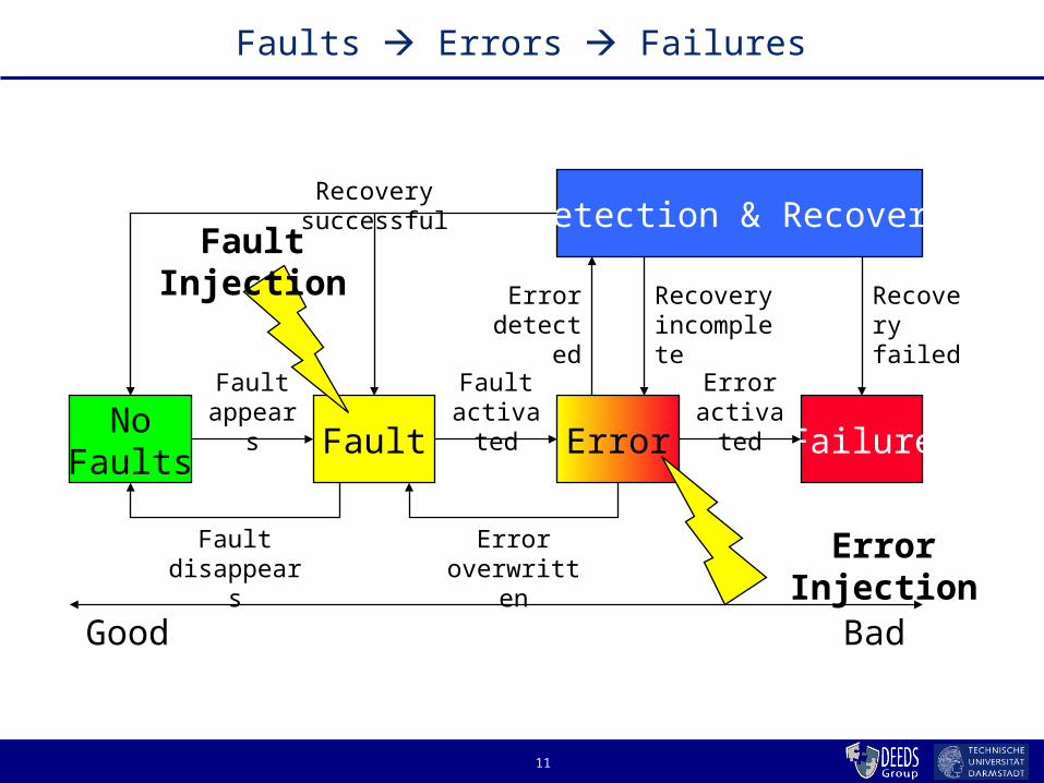
Faults Errors Failures

Fault Error Failure

Good Bad

Detection & Recovery

NoFaults

Fault appears

Fault activated

Error activated

Recovery failed

Fault disappears

Error overwritten

Recovery incomplete

Error detected

Recovery successful

Fault Injection

Error Injection

12

Basics of Fault Injection

Where: to apply change (location, abstraction/system level)

What: to inject (what should be injected/corrupted?) Which: trigger to use (event, instruction, timeout,

exception, code mutation?) When: to inject (corresponding to type of fault) How: often to inject (corresponding to type of fault) … What to record & interpret? To what purpose? How is the system loaded at the time of the

injection Applications running and their load (workload) System resources Real realistic synthetic workload

13

Various FI Approaches

Physical fault injection EMI, radiation, …

Simulated fault injection Injections into VHDL-model

Hardware fault-injection Pin-level injection Scan chains

Software implemented fault injection (SWIFI) Bit-flips, mutations Code and Data segments API’s, …

14

Coverage and Latency

Aim is to find characteristics of Event X Event X may be detection, recovery, etc.

Coverage of Event X Conditional probability of Event X occurring E.g. probability of error detection given that an error exists

in the system

Latency of Event X Time from the earliest (theoretically) possible occurrence

of Event X to the actual monitored occurrence E.g. time from error occurrence to error detection

15

Estimating Metrics in FI

Detection coverage = #detections/#injections Detection latency = mean (detection times) Recovery coverage = #recoveries/#detections Recovery latency = mean (recovery times)

16

Physical Fault Injection

Reproduce extreme environmental conditions EMI Radiation Heat Shock Voltage drops/spikes etc

Advantages “Real” faults Tangible Simple “test cases”

Disadvantages Difficult to control/repeat Needs at least a prototype

17

Simulation-based Fault Injection

Using a model of the system VHDL MatLab SystemC Spice

Advantages Usable during design Controllable

Disadvantages Requires a model Model accuracy? Slow

18

Simulated Fault Injection

Fault injection

Electrical level Logical level Functional level

Change currentChange voltage

Stuck at 0 or 1Inverted fault

Change CPU RegisterFlip memory bits, etc.

Electricalcircuits

Logic gatesFunctional

unitsPhysicalprocess

Logicoperation

19

Hardware-based Fault Injection

Inject faults using hardware (similar to physical) Pin-level injection Scan chains

Advantages Controllable Close to “real” faults

Disadvantages Requires special equipment Reachability?

20

SoftWare Implemented Fault Injection: SWIFI

Manipulate bits in memory locations and registers Emulation of HW faults Change text segment of processes

• Emulation of SW faults (bugs, defects) Dynamic: E.g., Op-code switch during operation Static: Change source code and recompile (a.k.a.

mutation)

21

SWIFI

PROS: No special hardware instrumentation Inexpensive and easy to control High observability (down to variables)

CONS: Only into locations accessible to software Instrumentation may disturb workload Difficult to observe short latency faults

Open questions: Is the injected fault representative of a “real” fault? Is the emulated/simulated environment (ops., load, tests)

representative of the real system?

22

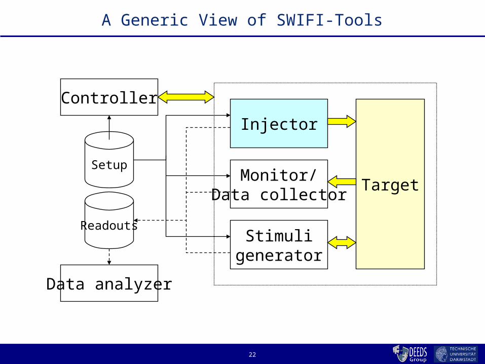
A Generic View of SWIFI-Tools

Controller

Data analyzer

Target

Injector

Stimuligenerator

Monitor/Data collector

Readouts

Setup

23

Many Tools Available

DEPEND, MEFISTO Evaluating HW/SW architectures using simulations

FERRARI, DOCTOR, RIFLE, Xception Evaluate tolerance against HW faults

DEFINE, FIAT, FTAPE Evaluate tolerance against HW and SW faults

MAFALDA, NFTAPE, PROPANE Evaluate effects of HW & SW faults and analyze error

propagation

Ballista OS Robustness testing

24

DEPEND and MEFISTO

Evaluation of system architectures E.g. validate TMR recovery protocols, synchronization

protocols etc.

Simulate system and components using SW DEPEND

uses object-oriented design for flexibility Models a system and it’s interactions and FTM’s

MEFISTO uses VHDL Testing of FTM’s Support for HW-based FI (validating Fault models)

25

FERRARI, DOCTOR and Xception

Evaluate system level effects of HW faults using SWIFI E.g. bit-errors in registers, address bus errors, etc.

FERRARI (Fault and ERRor Automatic Real-time Injector) Inject errors while applications are running Compare with golden run Registers, PC, Instruction type, branch and CC are targets

DOCTOR Injects CPU , memory and network faults Uses timeouts, traps and code mutations Used on distributed real-time systems

Xception (example on next slides) Uses debugging facilities in CPU’s

26

Xception

Goal: SWIFI using HW debugging support Minimizing intrusion using debugging interfaces Many fault triggers Detailed performance monitoring can be used Can affect any SW process (including kernel)

• No source code needed

Injector

Target App

Fault SetupExperiment

Manager

Module

Outputs

Faults

LogsResults

Fault Archive

Userspace

Kernelspace

27

Xception’s Fault Model

Duration Transient

Location Components inside processor

• Integer Unit, FPU, MMU, Buses, Registers, Branch processing

Trigger Temporal Opcode fetch, Operand load/store

Types Bit-flips Masks based on register/bus/memory sizes (e.g. 32 bits)

28

Xception

Data to collect Fault information System state information

• Instruction pointer etc Kernel and Application deviations

• Kernel error codes• Output of applications (workload)

Error detection status Performance monitoring information

29

Xception

Results for 4 node parallel computer running a Linda π calculation benchmark:

© J. Carreira et al, TOSE 24(2) 1998

Results for 4 node parallel computer running a Linda matrix multiplication benchmark (with FT algorithm):

© J. Carreira et al, TOSE 24(2) 1998

30

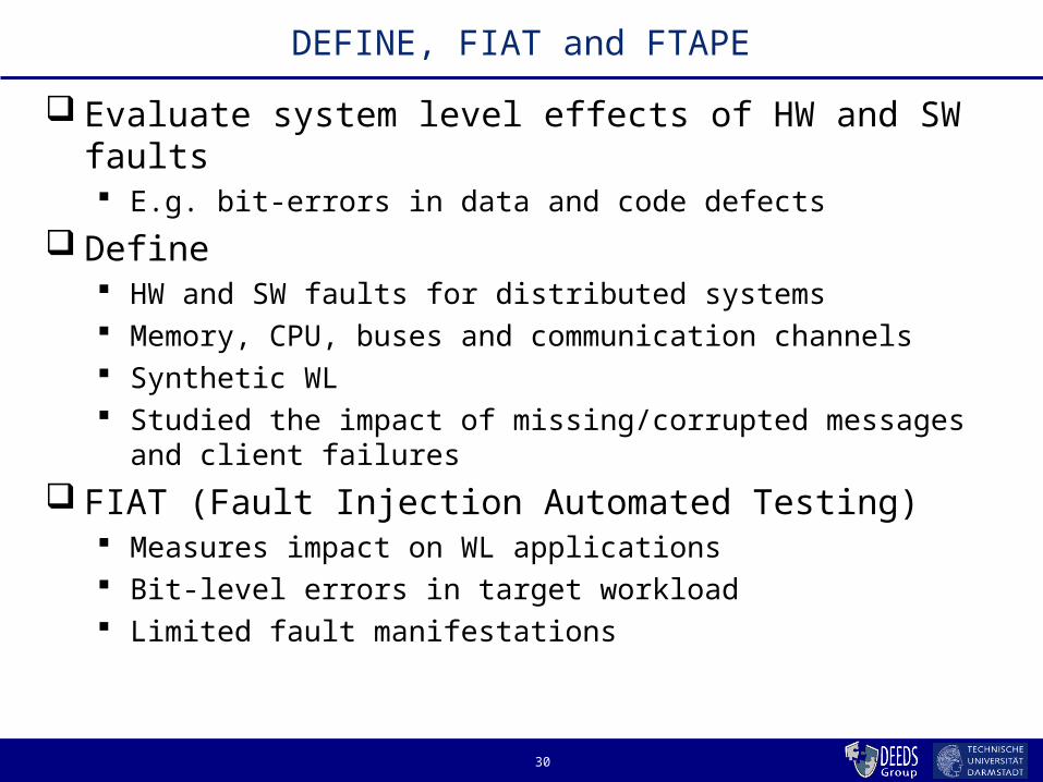
DEFINE, FIAT and FTAPE

Evaluate system level effects of HW and SW faults E.g. bit-errors in data and code defects

Define HW and SW faults for distributed systems Memory, CPU, buses and communication channels Synthetic WL Studied the impact of missing/corrupted messages and

client failures

FIAT (Fault Injection Automated Testing) Measures impact on WL applications Bit-level errors in target workload Limited fault manifestations

31

MAFALDA, NFTAPE and PROPANE

Evaluate effects of HW and SW faults, and analyze error propagation From system level down to variable level

Need instrumentation, but no HW-support MAFALDA focused on micro-kernels

Bit-flips in memory/data and API’s

NFTAPE tries to do everything in one tool! PROPANE purely software

32

Instrumentation Example (PROPANE)

int spherical_volume( double radius ){ double volume;

volume = 4.0 * (PI * pow(radius, 3.0)) / 3.0;

return volume;}

int spherical_volume( double radius ){ double volume;

/* Injection location for radius */ propane_inject( IL_SPHERE_VOL, &radius, PROPANE_DOUBLE );

/* Probe the value of radius */ propane_log_var( P_RADIUS, &radius );

volume = 4.0 * (PI * pow(radius, 3.0)) / 3.0;

/* Probe the value of volume */ propane_log_var( P_VOLUME, &volume );

return volume;}

Original codeOriginal code Instrumented codeInstrumented code

33

PROPANE

PROPANE = PROPagation ANalysis Environment

Highest Error RateHighest Error Rate

Lowest Error RateLowest Error Rate

ms_slot_nbr i

mscntpulscnt

slow_speed

stopped

IsValue

OutValue TOC2ADC

TCNTTIC1

PACNT

SetValue

CLOCK

PRES_S V_REG PRES_A

CALC

DIST_S

34

Code Mutations

Idea: Try to simulate real faults in binary code

1. Search real SW for faults2. Identify the fault patterns in the binaries3. Inject the patterns to your SW

35

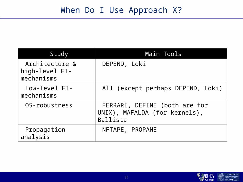
When Do I Use Approach X?

Study Main Tools

Architecture & high-level FI-mechanisms

DEPEND, Loki

Low-level FI-mechanisms

All (except perhaps DEPEND, Loki)

OS-robustness FERRARI, DEFINE (both are for UNIX), MAFALDA (for kernels), Ballista

Propagation analysis NFTAPE, PROPANE

36

Fault Injection

This is experimental and a statistical basis for establish a desired level of confidence in the system.

Keep in mind that:a) the statistical basis does not always apply to real systems esp.

SWb) statistically significant injections has little meaning if (a) appliesc) the injected fault is NOT the real fault

37

More Information

Iyer R., Tang D., ”Experimental Analysis of Computer System Dependability”, Chapter 5 in Pradhan’s book Fault-Tolerant Computer System Design, 1996

www.deeds.informatik.tu-darmstadt.de [Check papers on EPIC, Propane, M. Hiller’s PhD thesis]