1

Self-optimizing controlFrom key performance indicators to control of biological systems

Sigurd Skogestad

Department of Chemical Engineering

Norwegian University of Science and Technology (NTNU)

Trondheim

PSE 2003, Kunming, 05-10 Jan. 2004

2

Outline• Optimal operation

• Implememtation of optimal operation: Self-optimizing control

• What should we control?

• Applications– Marathon runner

– KPI’s

– Biology

– ...

• Optimal measurement combination

• Optimal blending example

Focus: Not optimization (optimal decision making)But rather: How to implement decision in an uncertain world

3

Optimal operation of systems

• Theory:– Model of overall system– Estimate present state– Optimize all degrees of freedom

• Problems: – Model not available and optimization complex– Not robust (difficult to handle uncertainty)

• Practice– Hierarchical system– Each level: Follow order (”setpoints”) given from level above– Goal: Self-optimizing

4

Process operation: Hierarchical structure

PID

RTO

MPC

5

What should we control?

y1 = c ? (economics)

y2 = ? (stabilization)

6

Self-optimizing Control

Self-optimizing control is when acceptable operation can be achieved using constant set points (c

s)

for the controlled variables c

(without re-optimizing when disturbances occur).

c=cs

7

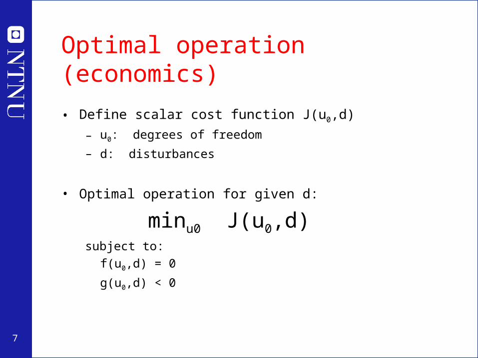
Optimal operation (economics)

• Define scalar cost function J(u0,d)

– u0: degrees of freedom

– d: disturbances

• Optimal operation for given d:

minu0 J(u0,d)subject to:

f(u0,d) = 0

g(u0,d) < 0

8

Implementation of optimal operation

• Idea: Replace optimization by setpoint control

• Optimal solution is usually at constraints, that is, most of the degrees of freedom u0 are used to satisfy “active constraints”, g(u0,d) = 0

• CONTROL ACTIVE CONSTRAINTS!– Implementation of active constraints is usually simple.

• WHAT MORE SHOULD WE CONTROL?– Find variables c for remaining

unconstrained degrees of freedom u.

9

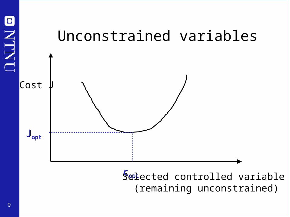
Unconstrained variables

Cost J

Selected controlled variable (remaining unconstrained)

ccoptopt

JJoptopt

10

Implementation of unconstrained variables is not trivial: How do we deal with uncertainty?

• 1. Disturbances d

• 2. Implementation error n

cs = copt(d*) – nominal optimization

nc = cs + n

d

Cost J Jopt(d)

11

Problem no. 1: Disturbance d

Cost J

Controlled variable ccoptopt(d(d**))

JJoptopt

dd**

d d ≠≠ dd**

Loss with constant value for c

) Want copt independent of d

12

Problem no. 2: Implementation error n

Cost J

ccss=c=coptopt(d(d**))

JJoptopt

dd** Loss due to implementation error for c

c = cs + n

) Want n small and ”flat” optimum

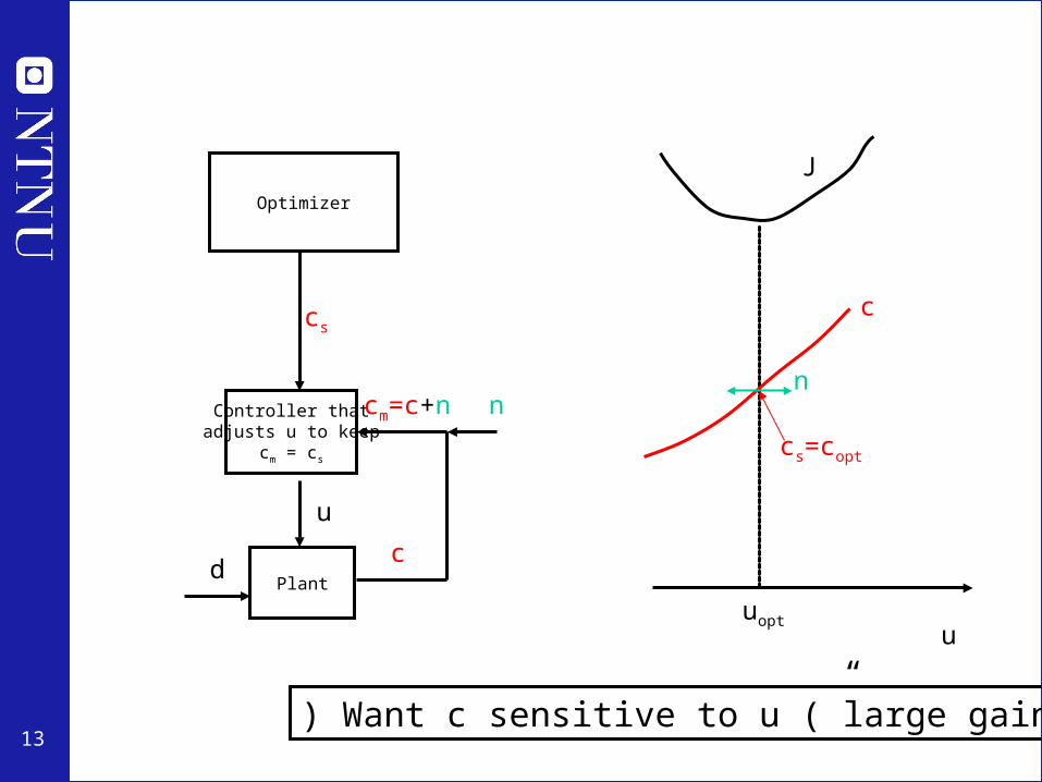
13

Optimizer

Controller thatadjusts u to keep

cm = cs

Plant

cs

cm=c+n

u

c

n

d

u

c

J

cs=copt

uopt

n

) Want c sensitive to u (”large gain”)

14

Which variable c to control?

• Define optimal operation: Minimize cost function J

• Each candidate variable c:

With constant setpoints cs compute loss L for expected disturbances d and implementation errors n

• Select variable c with smallest loss

15

Constant setpoint policy:Loss for disturbances (“problem 1”)

Acceptable loss ) self-optimizing control

16

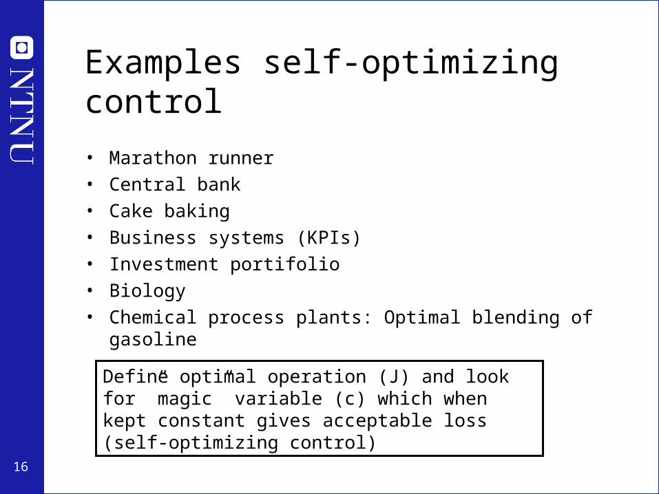
Examples self-optimizing control

• Marathon runner

• Central bank

• Cake baking

• Business systems (KPIs)

• Investment portifolio

• Biology

• Chemical process plants: Optimal blending of gasoline

Define optimal operation (J) and look for ”magic” variable (c) which when kept constant gives acceptable loss (self-optimizing control)

17

Self-optimizing Control – Marathon

• Optimal operation of Marathon runner, J=T– Any self-optimizing variable c (to control at constant

setpoint)?

18

Self-optimizing Control – Marathon

• Optimal operation of Marathon runner, J=T– Any self-optimizing variable c (to control at constant

setpoint)?• c1 = distance to leader of race

• c2 = speed

• c3 = heart rate

• c4 = level of lactate in muscles

19

Further examples

• Central bank. J = welfare. c=inflation rate (2.5%)• Cake baking. J = nice taste, c = Temperature (200C)• Business, J = profit. c = ”Key performance indicator (KPI), e.g.

– Response time to order– Energy consumption pr. kg or unit– Number of employees– Research spendingOptimal values obtained by ”benchmarking”

• Investment (portofolio management). J = profit. c = Fraction of investment in shares (50%)

• Biological systems:– ”Self-optimizing” controlled variables c have been found by natural

selection– Need to do ”reverse engineering” :

• Find the controlled variables used in nature• From this identify what overall objective J the biological system has been

attempting to optimize

20

Looking for “magic” variables to keep at constant setpoints.

How can we find them?

• Consider available measurements y, and evaluate loss when they are kept constant (“brute force”):

• More general: Find optimal linear combination (matrix H):

21

Optimal measurement combination (Alstad)

• Basis: Want optimal value of c independent of disturbances ) copt = 0 ¢ d

• Find optimal solution as a function of d: uopt(d), yopt(d)

• Linearize this relationship: yopt = F d • F – sensitivity matrix

• Want:

• To achieve this for all values of d:

• Always possible if

22

Example: Optimal blending of gasoline

Stream 1

Stream 2

Stream 3

Stream 4

Product 1 kg/s

Stream 1 99 octane 0 % benzene p1 = (0.1 + m1) $/kg

Stream 2 105 octane 0 % benzene p2 = 0.200 $/kg

Stream 3 95 → 97 octane 0 % benzene p3 = 0.120 $/kg

Stream 4 99 octane 2 % benzene p4 = 0.185 $/kg

Product > 98 octane < 1 % benzene

Disturbance

m1 = ? (· 0.4)

m2 = ?

m3 = ?

m4 = ?

23

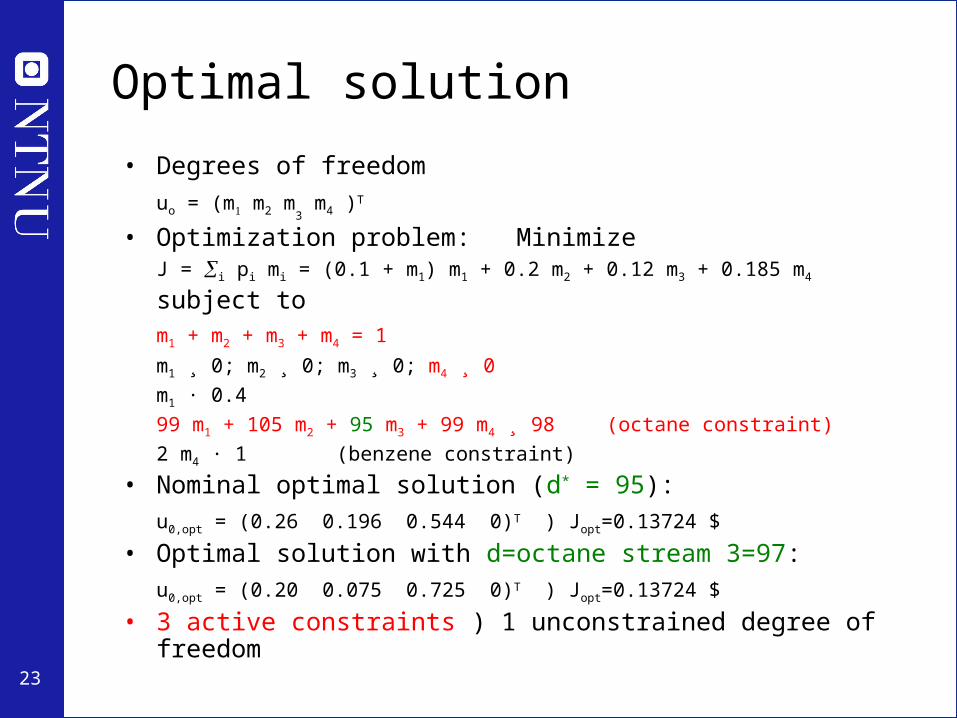
Optimal solution

• Degrees of freedom

uo = (m m2 m3 m4 )T

• Optimization problem: MinimizeJ = i pi mi = (0.1 + m1) m1 + 0.2 m2 + 0.12 m3 + 0.185 m4

subject tom1 + m2 + m3 + m4 = 1

m1 ¸ 0; m2 ¸ 0; m3 ¸ 0; m4 ¸ 0

m1 · 0.4

99 m1 + 105 m2 + 95 m3 + 99 m4 ¸ 98 (octane constraint)

2 m4 · 1 (benzene constraint)

• Nominal optimal solution (d* = 95):

u0,opt = (0.26 0.196 0.544 0)T ) Jopt=0.13724 $ • Optimal solution with d=octane stream 3=97:

u0,opt = (0.20 0.075 0.725 0)T ) Jopt=0.13724 $ • 3 active constraints ) 1 unconstrained degree of freedom

24

Implementation of optimal solution

• Available ”measurements”: y = (m1 m2 m3 m4)T

• Control active constraints:– Keep m4 = 0– Adjust one (or more) flow such that m1+m2+m3+m4 = 1– Adjust one (or more) flow such that product octane = 98

• Remaining unconstrained degree of freedom1. c=m1 is constant at 0.126 ) Loss = 0.00036 $

2. c=m2 is constant at 0.196 ) Infeasible (cannot satisfy octane = 98)

3. c=m3 is constant at 0.544 ) Loss = 0.00582 $

• Optimal combination of measurementsc = h1 m1 + h2 m2 + h3 ma

From optimization: mopt = F d where sensitivity matrix F = (-0.03 -0.06 0.09)T

Requirement: HF = 0 )

-0.03 h1 – 0.06 h2 + 0.09 h3 = 0This has infinite number of solutions (since we have 3 measurements and only ned 2):

c = m1 – 0.5 m2 is constant at 0.162 ) Loss = 0

c = 3 m1 + m3 is constant at 1.32 ) Loss = 0

c = 1.5 m2 + m3 is constant at 0.83 ) Loss = 0

• Easily implemented in control system

25

Example of practical implementation of optimal blending

• Selected ”self-optimizing” variable: c = m1 – 0.5 m2 • Changes in feed octane (stream 3) detected by octane controller (OC)• Implementation is optimal provided active constraints do not change • Price changes can be included as corrections on setpoint cs

FC

OC

mtot.s = 1 kg/s

mtot

m3

m4 = 0 kg/s

Octanes = 98

Octane

m2

Stream 2

Stream 1

Stream 3

Stream 4

cs = 0.162

0.5

m1 = cs + 0.5 m2

Octane varies

26

Conlusion

• Operation of most real system: Constant setpoint policy (c = cs)– Central bank– Business systems: KPI’s– Biological systems– Chemical processes

• Goal: Find controlled variables c such that constant setpoint policy gives acceptable operation in spite of uncertainty ) Self-optimizing control

• Method: Evaluate loss L = J - Jopt

• Optimal linear measurement combination: c = H y where HF=0

27

Engineering systems

• Most (all?) large-scale engineering systems are controlled using hierarchies of quite simple single-loop controllers – Large-scale chemical plant (refinery)

– Commercial aircraft

• 1000’s of loops

• Simple components: on-off + P-control + PI-control + nonlinear fixes + some feedforward

Same in biological systems

28

Good candidate controlled variables c (for self-optimizing control)

Requirements:

• The optimal value of c should be insensitive to disturbances (avoid problem 1)

• c should be easy to measure and control (rest: avoid problem 2)

• The value of c should be sensitive to changes in the degrees of freedom

(Equivalently, J as a function of c should be flat)

• For cases with more than one unconstrained degrees of freedom, the selected controlled variables should be independent.

Singular value rule (Skogestad and Postlethwaite, 1996):Look for variables that maximize the minimum singular value of the appropriately scaled steady-state gain matrix G from u to c