1

Robust Online Matrix Factorization forDynamic Background Subtraction

Hongwei Yong, Deyu Meng, Wangmeng Zuo, Lei Zhang

Abstract—We propose an effective online background subtraction method, which can be robustly applied to practical videos that havevariations in both foreground and background. Different from previous methods which often model the foreground as Gaussian orLaplacian distributions, we model the foreground for each frame with a specific mixture of Gaussians (MoG) distribution, which isupdated online frame by frame. Particularly, our MoG model in each frame is regularized by the learned foreground/backgroundknowledge in previous frames. This makes our online MoG model highly robust, stable and adaptive to practical foreground andbackground variations. The proposed model can be formulated as a concise probabilistic MAP model, which can be readily solved byEM algorithm. We further embed an affine transformation operator into the proposed model, which can be automatically adjusted to fita wide range of video background transformations and make the method more robust to camera movements. With using thesub-sampling technique, the proposed method can be accelerated to execute more than 250 frames per second on average, meetingthe requirement of real-time background subtraction for practical video processing tasks. The superiority of the proposed method issubstantiated by extensive experiments implemented on synthetic and real videos, as compared with state-of-the-art online and offlinebackground subtraction methods.

Index Terms—Background subtraction, mixture of Gaussians, low-rank matrix factorization, subspace learning, online learning.

F

1 INTRODUCTION

V IDEO processing is one of the main branches in imageprocessing and computer vision, which is targeted to

extract knowledge from videos collected from real scenes.As an essential and fundamental research topic in videoprocessing, background subtraction has been attracting in-creasing attention in the recent years. The main aim of back-ground subtraction is to separate moving object foregroundfrom the background in a video, which always makes thesubsequent video processing tasks easier and more efficient.Typical applications of background subtraction include ob-ject tracking [1], urban traffic detection [2], long-term scenemonitoring [3], video compression [4] and so on.

The initial strategies proposed to handle backgroundsubtraction are to directly distinguish background pixelsfrom foreground ones through some simple statistical mea-sures, like the median(mean) model [5], [6] and some his-togram models [7]. Later, more elaborate statistical models,like the MOG [8] and MOGG [9] models, were presented tobetter deliver the distributions of the image pixels located inthe background. These methods, however, ignore very use-ful video structure knowledge, like temporal similarity ofbackground scene and spatial contiguity of foreground ob-jects, and thus always cannot guarantee a good performanceespecially under complex scenarios. In recent decades, low-rank subspace learning models [10], [11] represent a newtrend and achieve state-of-the-art performance for this task

• Hongwei Yong and Deyu Meng (corresponding author) are with Schoolof Mathematics and Statistics and Ministry of Education Key Lab ofIntelligent Networks and Network Security, Xi’an Jiaotong University,Shaanxi, P.R. China. (e-mail:dymeng@mail.xjtu.edu.cn).

• Wangmeng Zuo is with School of Computer Science and Technology,Harbin Institute of Technology, Harbin P.R. China.

• Lei Zhang is with the Biometrics Research Center, Department of Com-puting, the Hong Kong Polytechnic University, Kowloon, Hong Kong.

due to their better consideration of video structure knowl-edge both in foreground and background. Especially, thesemethods assume a rational low-rank structure for videobackgrounds, which encodes the similarity of video back-grounds along time, and mostly consider useful prior fore-ground structures, like sparsity and spatial continuity. Sometypical models along this line are [12], [13], [14], [15], [16].

Albeit substantiated to be effective in some video se-quences with fixed lengthes, there is still a gap of uti-lizing such offline methodologies to real video processingapplications. Specifically, it is known that the amount ofvideos nowadays is dramatically increasing from surveil-lance cameras scattered all over the world. This not onlymakes it critical to calculate background subtraction fromsuch large amount of videos, but also urgently requiresto construct real-time techniques to handle the constantlyemerging videos. Online subspace learning has thus becomean important issue to alleviate this efficiency issue. Veryrecently, multiple online methods for background subtrac-tion have been designed [13], [17], [18], which speedup thecomputation by gradually updating the low-rank structureunder video background through incrementally treatingonly one frame at a time. Such online amelioration alwayssignificantly speeds up the calculation for the task, andmakes it possible to efficiently handle the task even in realtime under large-scaled video contexts.

However, the current online background subtractiontechniques still have evident defects when being appliedto real videos. On one hand, most current methods as-sume a low-rank structure for video background whileneglect frequently-occurring dynamic camera jitters, suchas translation, rotation, scaling and light/shade change,across video sequences. Such issues, however, always hap-pen in real life due to camera status switching or cir-

arX

iv:1

705.

1000

0v1

[cs

.CV

] 2

8 M

ay 2

017

2

(a) Bootstrap sequence (b) Campus sequenceFig. 1. Background subtraction results by the proposed OMoGMF method on (a) bootstrap sequence; (b) campus sequence. First row (from leftto right): Original frame, noise and background extracted by the proposed method. Second row: Three noise components (after scale processing)extracted by the method, corresponding to the moving object, the shadow along the object, weak camera noise (for (a)) and the moving object,leaves shaking variance, weak camera noise (for (b)), respectively.

cumstance changing over time and tend to damage theconventional low-rank assumption for video backgrounds.Actually, the image sequence formed by slightly translat-ing/rotating/scaling each of its single images will alwayshave no low-rank property at all. Thus the performanceof current methods tend to be evidently degenerated insuch background-changing cases, and it should be critical tomake the online learning capable of adapting such camerajitters.

On the other hand, all current online methods for thistask used a fixed loss term, e.g., L2 or L1 losses, in theirmodels, which implicitly assume that noises (foregrounds)involved in videos follow a fixed probability distribution,e.g., Gaussian or Laplacian. Such assumption, however, de-viates from the real scenarios where the foregrounds alwayshave dramatic variations over time. E.g., in some framesthere are no foreground objects existed, where noises canbe properly modeled as a Gaussian (i.e., L2-norm loss), inother cases there might be an object occluding a large areain the background, where noises should be better modeledas a long tailed Laplacian (i.e., L1-norm loss), while in moreoften cases, the foreground might contain multiple modal-ities of noises, as those depicted in Fig. 1, which requireto consider more complex noise models. The ignoring ofsuch important insight of video foreground diversity alwaysmakes current methods not robust enough to finely adaptreal-time foreground/noise variations in practice.

To alleviate the aforementioned issues, in this work wepropose a new online background subtraction method. Thecontribution can be summarized as follows:

Firstly, instead of using fixed noise distribution through-out all video frames as conventional, the proposed methodmodels the noise/foregound of each video frame as a sep-arate mixture of Gaussian (MoG) distribution, regularizedby a penalty for enforcing its parameters close to thosecalculated from the previous frames. Such penalty can beequivalently reformulated as the conjugate prior, encodingthe noise knowledge previous learned, for the MoG noiseof current frame. Due to the good approximation capabilityof MoG to a wide range of distributions, our method canfinely adapt video foreground variations even when thevideo noises are with dynamic complex structures.

Secondly, we have involved an affine transformationoperator for each video frame into the proposed model,

which can be automatically fitted from the temporal videocontexts. Such amelioration makes our method capable ofadapting wide range of video background transformations,like translation, rotation, scaling and any combinationsof them, through properly aligning video backgrounds tomake them residing on a low-rank subspace in an onlinemanner. The proposed method can thus perform evidentlymore robust on the videos with dynamical camera jitters ascompared with previous methods.

Thirdly, the efficiency of our model is further enhancedby embedding the sub-sampling technique into calculation.By utilizing this strategy, the proposed method can beaccelerated to execute more than 250 frames per secondon average (in Matlab platform), while still keeping a goodperformance in accuracy, which meets the real-time require-ment for practical video processing tasks. Besides, attributedto the MoG noise modeling methodology, the separatedforeground layers always can be interpreted with certainphysical meanings, as shown in Fig. 1, which facilitates usto get more intrinsic knowledge under video foreground.

Fourthly, our method can be easily extended to othersubspace alignment tasks, like image alignment and videostabilization applications. This implies the good generaliza-tion of the proposed method.

The paper is organized as follows: Section 2 reviewssome related works. Section 3 proposes our model andrelated algorithms. Its sub-sampling amelioration and otherextensions are also introduced in this section. Section 4shows experimental results on synthetic and real videos,to substantiate the superiority of the proposed method.Discussions and concluding remark are finally given.

2 RELATED WORK

2.1 Low Rank Matrix Factorization

low rank matrix factorization (LRMF) is one of themost commonly utilized subspace learning approaches forbackground subtraction. The main idea is to extract the low-rank approximation of the data matrix from the productof two smaller matrices, corresponding to the basis matrixand coefficient matrix, respectively. Based on the loss termsutilized to measure the approximation extent, the LRMFmethods can be mainly categorized into three classes. L2-LRMF methods [19] utilizes L2-norm loss in the model, im-

3

plicitly assuming that the noise distribution in data is Gaus-sian. Typical L2-LRMF methods include weighted SVD [20],WLRA [21], L2-Wiberg [22] and so on. To make the LRMFmethod less sensitive to outliers, some robust loss functionshave been utilized, in which the L1-LRMF methods are themost typical ones. The L1-LRMF utilizes the L1 loss term,implying that the data noise follows a Laplacian distribu-tion. Due to the heavy-tailed characteristic of Laplacian,such method always could perform more robust in thepresence of heavy noises/outliers. Some commonly adoptedL1-LRMF methods include: L1Wiberg [23], RegL1MF [24],PRMF [13] and so on. To adapt more complex noise configu-rations in data, several models have recently been proposedto encode the noise as a parametric probabilistic model,and accordingly learn the loss term as well as the modelparameters simultaneously. In this way, the model is capableof adapting wider range of noises as compared with theprevious ones with fixed noise distributions. The typicalmethods in this category include the MoG-LRMF [16], [25]and MoEP-LRMF [26] methods, representing noise distri-butions as a MoG and a mixture of exponential powerdistributions, respectively. Despite having been verified tobe effective in certain scenarios, these methods implicitlyassume stable backgrounds across all video frames and fixednoise distribution for foreground objects throughout videos.As we have analyzed, neither is proper for practically col-lected videos, which tends to degenerate their performance.

2.2 Background Subtraction

As a fundamental research topic in video processing,background subtraction has been investigated widely nowa-days. The initial strategies mainly assumed that the dis-tribution (along time) of background pixels can be distin-guished from that of foreground ones. Thus by judgingif a pixel is significantly deviated from the backgroundpixel distribution, we can easily categorize if a pixel islocated in background/foreground. The simplest methodsalong this line directly utilize a statistic measure, like themedian [6] or mean [5] to encode background knowledge.Later more complex distributions on background pixels,like MOG [8], MOGG [9] and so on [27] [28], are moreeffective. The disadvantage of these methods is that theyneglect useful video structure knowledge, e.g., temporalsimilarity of background scene and spatial contiguity offoreground objects, and thus always cannot guarantee agood performance practically. Low-rank subspace learningmodels represent the recent state-of-the-art for this task ongeneral surveillance videos due to their better considerationof video structures. These methods implicitly assume stablebackground in videos, which are naturally with a low-rank structure. Multiple models have been raised on thistopic recently, typically including PCP [12], GODEC [15],and DECOLOR [14]. Albeit obtaining state-of-the-art per-formance in some benchmark video sets, these methodsstill cannot be effectively utilized in real-time problems dueto both their simplified assumptions in video backgrounds(with stationary background scenes) and foreground (withfixed type of noise distributions along time). They also tendto encounter efficiency problem for real-time requirements,especially for large scaled videos. Very recently, some deepneural network works [29], [30] were also attempted on

the task against specific scenes, while need large amountof pre-annotations. In this paper we mainly focus on han-dling general surveillance videos without any supervisedforeground/background knowledge, and thus have not con-sidered this approach in our experiment comparison.

2.3 Online Subspace LearningNowadays, it has been attracting increasing attention to

design online subspace learning method to handle real-timebackground subtraction issues [31], [32]. The basic idea isto calculate only one frame at a time, and gradually ame-liorate the background based on the real-time video vari-ations. The state-of-the-art methods along this line includeGRASTA [17], OPRMF [13], GOSUS [18], PracReProCS [33]and incPCP [34], [35]. GRASTA used a L1 norm loss for eachframe to encode sparse foreground objects, and employedADMM strategy for subspace updating. Similar to GRASTA,OPRMF also optimized a L1-norm loss term while addedregularization terms to subspace parameters to alleviateoverfitting. GOSUS designed a more complex loss term toencode the structure of video foreground, and the updatingalgorithm is designed similar to that of GRASTA. Besides,PracReProCS and incPCP were recently proposed, which arethe incremental extensions of the classical PCP algorithm.

However, these methods are still deficient due to theirinsufficient consideration on variations both in backgroundand foreground in real videos. On one hand, they assume alow-rank structure for the video background, which ignoresvery often existed background changes and camera jittersacross video sequences. On the other hand, they all fixthe loss term in their models, which implicitly assumesthat noise involved in data is generated from a fixedprobability distribution. This, however, under-estimates thetemporal variations of the foreground objects in videos.That is, in some frames the foreground signals might bevery weak while in others they might be very evident.The noise distributions are thus not fixed while varyingacross video frames. The underestimation of both fore-ground/background knowledge incline to degenerate theircapability for real online tasks.

2.4 Robust Subspace AlignmentRecently, multiple subspace learning strategies have

been constructed to learn transformation operators on videoframes to make the methods robust to camera jitters. Atypical method is RASL (robust alignment by sparse andlow-rank decomposition) [36], which poses the learning oftransformation operators into the classical robust principalcomponent analysis (RPCA) model, and simultaneouslyoptimize the parameters involved in such operators as wellas the low-rank (background) and sparse (foreground) ma-trices. Other similar works are extended by [37], [38], [39].However, such batch-mode methods are generally slow torun and can only deal with moderate scaled videos. To thisissue, incPCP TI [40] is extended from incPCP by takingtranslation and rotation into consideration to deal withimage rigid transformation. t-GRASTA [41] realized a moregeneral subspace alignment by embedding an affine trans-formation operator into online subspace learning. Althoughcapable of speeding up the offline methods, the methodsutilized a simple L1-norm loss to model foreground. This

4

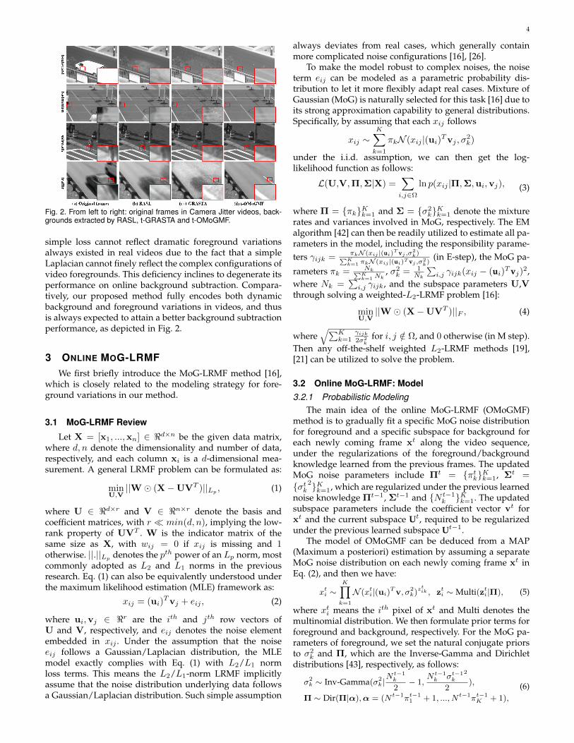
Fig. 2. From left to right: original frames in Camera Jitter videos, back-grounds extracted by RASL, t-GRASTA and t-OMoGMF.

simple loss cannot reflect dramatic foreground variationsalways existed in real videos due to the fact that a simpleLaplacian cannot finely reflect the complex configurations ofvideo foregrounds. This deficiency inclines to degenerate itsperformance on online background subtraction. Compara-tively, our proposed method fully encodes both dynamicbackground and foreground variations in videos, and thusis always expected to attain a better background subtractionperformance, as depicted in Fig. 2.

3 ONLINE MOG-LRMFWe first briefly introduce the MoG-LRMF method [16],

which is closely related to the modeling strategy for fore-ground variations in our method.

3.1 MoG-LRMF Review

Let X = [x1, ...,xn] ∈ <d×n be the given data matrix,where d, n denote the dimensionality and number of data,respectively, and each column xi is a d-dimensional mea-surement. A general LRMF problem can be formulated as:

minU,V||W (X−UVT )||Lp , (1)

where U ∈ <d×r and V ∈ <n×r denote the basis andcoefficient matrices, with r min(d, n), implying the low-rank property of UVT . W is the indicator matrix of thesame size as X, with wij = 0 if xij is missing and 1otherwise. ||.||Lp

denotes the pth power of an Lp norm, mostcommonly adopted as L2 and L1 norms in the previousresearch. Eq. (1) can also be equivalently understood underthe maximum likelihood estimation (MLE) framework as:

xij = (ui)Tvj + eij , (2)

where ui,vj ∈ <r are the ith and jth row vectors ofU and V, respectively, and eij denotes the noise elementembedded in xij . Under the assumption that the noiseeij follows a Gaussian/Laplacian distribution, the MLEmodel exactly complies with Eq. (1) with L2/L1 normloss terms. This means the L2/L1-norm LRMF implicitlyassume that the noise distribution underlying data followsa Gaussian/Laplacian distribution. Such simple assumption

always deviates from real cases, which generally containmore complicated noise configurations [16], [26].

To make the model robust to complex noises, the noiseterm eij can be modeled as a parametric probability dis-tribution to let it more flexibly adapt real cases. Mixture ofGaussian (MoG) is naturally selected for this task [16] due toits strong approximation capability to general distributions.Specifically, by assuming that each xij follows

xij ∼K∑k=1

πkN (xij |(ui)Tvj , σ2k)

under the i.i.d. assumption, we can then get the log-likelihood function as follows:

L(U,V,Π,Σ|X) =∑i,j∈Ω

ln p(xij |Π,Σ,ui,vj), (3)

where Π = πkKk=1 and Σ = σ2kKk=1 denote the mixture

rates and variances involved in MoG, respectively. The EMalgorithm [42] can then be readily utilized to estimate all pa-rameters in the model, including the responsibility parame-ters γijk =

πkN (xij |(ui)T vj ,σ

2k)∑K

k=1 πkN (xij |(ui)T vj ,σ2k)

(in E-step), the MoG pa-

rameters πk = Nk∑Kk=1Nk

, σ2k = 1

Nk

∑i,j γijk(xij − (ui)Tvj)2,

where Nk =∑i,j γijk, and the subspace parameters U,V

through solving a weighted-L2-LRMF problem [16]:

minU,V||W (X−UVT )||F , (4)

where√∑K

k=1γijk2σ2

kfor i, j /∈ Ω, and 0 otherwise (in M step).

Then any off-the-shelf weighted L2-LRMF methods [19],[21] can be utilized to solve the problem.

3.2 Online MoG-LRMF: Model3.2.1 Probabilistic Modeling

The main idea of the online MoG-LRMF (OMoGMF)method is to gradually fit a specific MoG noise distributionfor foreground and a specific subspace for background foreach newly coming frame xt along the video sequence,under the regularizations of the foreground/backgroundknowledge learned from the previous frames. The updatedMoG noise parameters include Πt = πtkKk=1, Σt =

σtk2Kk=1, which are regularized under the previous learned

noise knowledge Πt−1, Σt−1 and N t−1k Kk=1. The updated

subspace parameters include the coefficient vector vt forxt and the current subspace Ut, required to be regularizedunder the previous learned subspace Ut−1.

The model of OMoGMF can be deduced from a MAP(Maximum a posteriori) estimation by assuming a separateMoG noise distribution on each newly coming frame xt inEq. (2), and then we have:

xti ∼K∏k=1

N (xti|(ui)Tv, σ2k)z

tik , zti ∼ Multi(zti|Π), (5)

where xti means the ith pixel of xt and Multi denotes themultinomial distribution. We then formulate prior terms forforeground and background, respectively. For the MoG pa-rameters of foreground, we set the natural conjugate priorsto σ2

k and Π, which are the Inverse-Gamma and Dirichletdistributions [43], respectively, as follows:

σ2k ∼ Inv-Gamma(σ2

k|N t−1k

2− 1,

N t−1k σt−1

k

2

2),

Π ∼ Dir(Π|α),α = (N t−1πt−11 + 1, ..., N t−1πt−1

K + 1),

(6)

5

Fig. 3. The graphical model for OMoGMF.

where N t−1 =∑Kk=1N

t−1k , πt−1

k = N t−1k /N t−1. It can be

calculated that the maximum of the above conjugate priorsare Σt−1 and Πt−1. This implies that the priors implicitlyencode the previously learned noise knowledge into theOMoGMF model, and help rectify the MoG parameters ofthe current frame not too far from the previous learned ones.For the subspace of background, a Gaussian distributionprior can be easily set for its each row vector:

ui ∼ N (ui|uit−1,1

ρAt−1i ), (7)

where 1ρAt−1

i is a positive semi-definite matrix.This facili-tate the to-be-learned subspace variable U being well reg-ularized by the previously learned Ut−1. Details of how toset At−1

i will be introduced in Sec. 3.4. To make a completeBayesian model, we also set a noninformative prior p(v) forv, which does not intrinsically influence the calculation. Thefull graphical model is depicted as Fig. 3.

3.2.2 Objective Function

All hyperparameters are denoted by Θt−1, and aftermarginalizing the latent variable zt, we can get the posteriordistribution of Π,Σ,v,U in the following form:

p(Π,Σ,v,U|xt,Θt−1) ∝p(xt|Π,Σ,v,U)p(Σ|Θt−1)p(Π|Θt−1)p(U|Θt−1)p(v).

(8)

Based on the MAP principle, we can get the followingminimization problem for calculating Πt,Σt,vt,Ut:

Lt(Π,Σ,v,U) = − ln p(xt|Π,Σ,v,U) +RtF (Π,Σ) +RtB(U), (9)

where

ln p(xt|Π,Σ,v,U) =∑i

ln(

K∑k=1

πkN (xti|(ui)Tv, σ2k)),

RtF (Π,Σ) =

K∑k=1

N t−1k (

1

2

σt−1k

2

σ2k

+ lnσk)−N t−1K∑k=1

πt−1k lnπk,

RtB(U) = ρ

d∑i=1

(ui − uit−1)T (At−1

i )−1(ui − uit−1).

In the above problem, the first term is the likelihood term,which enforces the learned parameters adapt to the currentframe xt. The second term RtF (Π,Σ) is the regularizationterm for noise distribution, whose function can be moreintuitively interpreted by the following equivalent form:

RtF (Π,Σ) =

K∑k=1

N t−1k DKL(N (x|0, σt−1

k

2)||N (x|0, σk2))

+N t−1DKL(Multi(z|Πt−1)||Multi(z|Π)) + C

= N t−1DKL(p(x, z|Πt−1,Σt−1)||p(x, z|Π,Σ)) + C,

(10)

where p(x, z|Π,Σ) =∏Kk=1 πk

zkN (x|0, σk2)zk , DKL(·||·)denotes the KL divergence between two distributions. It canbe evidently observed that RtF (Π,Σ) functions to rectifythe foreground distribution on the current tth frame (withparameters Π,Σ) to approximate the previously learnedone (with parameters Πt−1,Σt−1). Besides, the third termRtB(U) in (9) corresponds to a Mahalanobis distance be-tween each row vector of U to that of Ut−1, thus functioningto rectify the current learned subspace by the previouslylearned one. The compromising parameter N t−1 and ρ con-trol the strength of the priors, and their physical meaningsand setting manners will be introduced in Sec. 3.4.

To easily compare differences of our model with theprevious ones, we list typical models along this researchline, as well as ours, in Table 1.

3.3 Online MoG-LRMF: Algorithm

The online-EM algorithm can be readily utilized for solv-ing the OMoGMF model (9), by alternatively implementingthe following E-step and M-step on a new frame sample xt.

Online E Step: As the traditional EM strategy, this stepaims to estimate the expectation of posterior probability forlatent variable ztik, which is also known as responsibility γtik.The updating equation is as follows:

E(ztik) = γtik =πkN (xti|(ui)Tv, σk2)∑Kk=1 πkN (xti|(ui)Tv, σk2)

. (11)

Online M Step: On updating MoG parameters Π,Σ, weneed to minimize the following sub-optimization problem:

L′t(Π,Σ) = −Eztln p(xt, zt|Π,Σ,v,U)+RtF (Π,Σ). (12)

The closed-form solution is1:

πk = πt−1k − N

N(πt−1k − πk);

σk2 = σt−1

k

2 − Nk

Nk(σt−1k

2 − σk2)

(13)

whereN = d; Nk =

d∑i

γtik; πk =Nk

N;

σk2 =

1

Nk

d∑i=1

γtik(xti − (ui)Tv)2);

N = N t−1 +N ;Nk = N t−1k +Nk.

(14)

On updating coefficient parameter v, we need to solvethe sub-optimization problem of (9) with respect to v as:

minv||wt (xt −Uv)||2F , (15)

where each element of wt is wti =√∑K

k=1γtik

2σk2 for i =

1, 2, ..., d. This problem is a weighted least square problem,and has the closed-form solution as:

v = (UT diag(wt)2U)−1UT diag(wt)2xt. (16)

1. Inference details are listed in the supplementary material (SM).

6

TABLE 1Model comparison of typical subspace-based background subtraction methods

Method Foreground/BackgroundDecomposition Objective Function Constraint/Basic Assumption Implementation Scheme

RPCA [12] X = L + S minL,S ||L||∗ + λ||S||1 No OfflineGODEC [15] X = L + S + E minL,S ||E||2F rank(L) ≤ K, card(S) ≤ s Offline

RegL1 [24] X = UVT + S minU,V ||S||1 + λ||V||∗ UT U = I OfflinePRMF [13] X = UVT + E minU,V − ln p(X|U,V) + λ1||U||2F + λ2||V||2F eij ∼ L(e|0, λ) Offline

DECOLOR [14] X = L + EminL,S ||S⊥ E||2F + λ1||L||∗

+λ2||S||1 + λ3||S||TVsij ∈ 0, 1 Offline

GRASTA [17] xt = Uv + s minv ||s||1 UT U = I Online: Heuristically update UOPRMF [13] xt = Uv + e minv − ln p(xt|U,v) + λ||v||22 ei ∼ L(e|0, λ) Online: Heuristically update U

GOSUS [18] xt = Uv + s + e minv ||e||22 +∑L

l=1 λl||Dls||2 UT U = I Online: Heuristically update U

OMoGMF xt = Uv + eminΠ,Σ,v,U− ln p(xt|Π,Σ,v,U)

+RtF (Π,Σ) +Rt

B(U)ei ∼

∑Kk=1 πkN (e|0, σ2

k) Online: Optimize U

On updating the subspace parameter U, we need tosolve the following sub-problem of (9):

L′t(U) = −Eztln p(xt, zt|Π,Σ,v,U)+RtB(U)

= ||wt (xt −Uvt)||2F +Rtb(U),(17)

and it has closed-form solution for each its row vector as:

uti =(ρ(At−1

i )−1 + wti2vtvt

T)−1

(ρ(At−1i )−1ut−1

i +wti2xtiv

tT ).

In order to get a simple updating rule, we set

(Ati)−1 = ρ(At−1

i )−1 + wti2vtvt

T;

bti = ρ(At−1i )−1ui

t−1 + wti2xtiv

tT ,(18)

and then we have uit = At

ibti. By using matrix inverse

equation [43] and the equation uit−1 = At−1

i bt−1i , the

update rules for Ati and bti can be reformulated as:

Ati =

1

ρ

(At−1i − wti

2At−1i vtvt

TAt−1i

ρ+ wti2vtTAt−1

i vt

);

bti = ρbt−1i + wti

2xtiv

t.

(19)

Thus in each step of updating Ut, we only need to saveAt−1

i di=1, bt−1i di=1 calculated in the last step, which only

needs fixed storage memory. Note that since the matrixinverse computations are avoided in the above updatingequations, the efficiency of the algorithm is guaranteed.

Since the subspace, representing the background knowl-edge, changes relatively slowly along the video sequence,we only fine-tune U once after recursively implementing theabove E-M steps on updating γtikik, Πt, Σt, and vt untilconvergence for each new sample xt under fixed subspaceUt−1. The subspace can then be fine-tuned to adjust thetemporal background change in this video frame. Note thatthere are only simple computations involved in the aboveupdating process, except that in (16), we need to computethe inverse of a r × r matrix. In the background subtractioncontexts, the rank r is generally with a small value and farless than d, n. We thus can very efficiently calculate thismatrix inverse in general.

The OMoGMF algorithm can then be summarized inAlgorithm 1. About initialization, we need a warm-startfor starting our algorithm by running PCA on a smallbatch of starting video frames to get an initial subspace,employing MoG algorithm on the extracted noise to getinitial MoG parameters, and calculating the initial Aidi=1,bidi=1 for subspace learning.

Algorithm 1 [OMoGMF] online MoG-LRMF

Input: the MoG parameters: Πt−1,Σt−1, N t−1; model vari-ables: At−1

i di=1, bt−1i di=1, Ut−1; data: xt

Initialization: Π,Σ = Πt−1,Σt−1, vt

1: while not converged do2: Online E-step: compute γtik by (11)3: Online M-step: compute Π,Σ, N by (13) and v by (16)4: end while5: for each uti , i = 1, 2, ..., d do6: compute At

idi=1, btidi=1 by (19)7: compute uti by uti = At

ibti

8: end forOutput: Πt,Σt, N t, vt, At

idi=1, btidi=1, Ut.

3.4 Several remarks

On relationship between conjugate prior and KL diver-gence: Actually we can prove a general result to understandthe conjugate prior as an equivalent KL divergence regular-ization. For the fully exponential family distributions, wehave the following theorem2:Theorem 1 If a distribution p(x|θ) belongs to the full exponen-tial family with the form: p(x|θ) = η(θ)exp(θTφ(x)), and itsconjugate prior follows: p(θ|X , γ) = f(X , γ)η(θ)γexp(γθTX ),

then we have:

ln p(θ|X , γ) = −γDKL(p(x|θ∗)||p(x|θ)) + C,

where θ∗ = argmaxθ p(θ|X , γ) and C is a constant indepen-dent of θ.

Since both Gaussian and multinomial distributions be-long to the full exponential family, both conjugate priorsin (6) can be written in their equivalent KL divergence ex-pressions (10). We prefer to use the latter form in our studysince it can more intuitively deliver the noise regularizationinsight underlying our model in a deterministic manner.

On relationship to batch-mode model: Under the modelsetting of (9) (especially for the two regularization termsRtF (Π,Σ) and RtB(U)), there is an intrinsic relationshipbetween our online model incrementally implemented oncurrent sample xt with a batch-mode one on all learnedsamples xjtj=1, as described in the following theorem:Theorem 2 By setting N t−1 = (t−1)d and ρ = 1, minimizing

2. All proofs are presented in SM due to page limitation.

7

Frame index

Fig. 4. Tendency curves of the largest variance (σt1)2(with scale 10−2)

and ||Ut||F (with scale 103) along time under different values of Nt−1

and ρ, respectively, for curtain sequence. Typical video frames andsome foregrounds extracted by our method along time are also depicted.

(12) for Π,Σ and (17) for U are equivalent to calculating:

Πt,Σt = argmaxΠ,Σ

t∑j=1

ln p(xj , zj |Π,Σ,vj ,Uj),

Ut = argmaxU

t∑j=1

ln p(xj , zj |Πj ,Σj ,vj ,U),

(20)

respectively. Moreover, under these settings, it holds that:

||Σt −Σt−1||F ≤ O(1

t), ||Πt −Πt−1||F ≤ O(

1

t),

||Ut −Ut−1||F ≤ O(1

t).

(21)

The above result demonstrates the batch-mode understand-ing of our online learning schemes, under fixed previouslylearned variables (zj ,vj ,Uj ,Πj ,Σjt−1

j=1), which have notbeen stored in memory in the online implementation man-ner and cannot be re-calculated on previous frames.

On parameters N t−1 and ρ : Although the naturalchoices for them are N t−1 = (t − 1)d and ρ = 1 basedon Theorem 2, under these settings, the prior knowledgelearned from previous frames will be gradually accumu-lated (note that the value of N t−1 will increase to infinity),and the function of the likelihood term (i.e., the effect of thecurrent frame) will be more and more alleviated with time.However, as the motivation of this work, we expect that ourmethod can consistently fit the foreground variations anddynamically adapt the noise changes with time, and thushope that the likelihood term can constantly play roles inthe computation. In our algorithm, we just easily setN t−1 asa fixed constant Kd (N t−1

k = N t−1πt−1k correspondingly),

meaning that we dominate the adjacent K frames to rectifythe online parameter updating of the current frame. Inpractical cases, a moderate K (e.g., we set it as 50 in all ourexperiments) is preferred to make the method adaptivelyreflect temporal variations of video foreground, while nottoo sensitive to single frame change, as clearly depictedin Fig. 4. Similarly, we easily set ρ as 0.98 throughout ourexperiments to let the updated subspace slightly lean to thecurrent frame.

3.5 Efficiency and Accuracy AmeliorationWe then introduce two useful techniques to further en-

hance the efficiency and accuracy of the proposed method.

3.5.1 Sub-sampling

It can be shown that a large low-rank matrix can bereconstructed from a small number of its entries [44] undercertain low-rank assumption. Inspired by some previous at-tempts [17] on this issue, we also prefer to use sub-samplingtechnique to further improve efficiency of our method.

For a newly coming frame x, we randomly sample someof its entries to get the sub-sampling data xΩ, where Ω isthe index set of the sampled entries, and then we only usexΩ to update the parameters involved in our model. Theupdating of MoG parameters Π and Σ is similar to theoriginal method, and v can be solved under the sampledsubspace UΩ. While for U, we only need to update its rowentries on Ω through using Aii∈Ω and bii∈Ω.

Generally speaking, the sub-sampling rate is inverselyproportional to the performance of our method, and wethus need to find a trade-off between efficiency and accuracyin real cases. E.g., in evidently low-rank background cases,the sampling rate should be larger while for scenes withcomplex backgrounds across videos, we need to samplemore data entries to guarantee accuracy.

3.5.2 TV-norm regularization

The foreground is defined as any objects which areoccluded before the background during a period of time. Inreal-world scenes, as we know, one foreground object oftenappears in a continuous shape and the region of one objectgenerally is with an evident spatial smoothness. In ouronline method, we also consider such spatial smoothness tofurther improve its accuracy on foreground object detection.

There are several strategies to encode the smoothnessproperty of an image, e.g., Markov random field (MRF) [3],[45], [46], Total Variation (TV) minimization [4], [47], andstructure sparsity [18], [48]. Considering effectiveness andefficiency, we employ the TV-minimization approach in ourmethod. For a foreground frame obtained by our method,we calculate the following TV-minimization problem:

FG′ = argminF

1

2||F− FG||22 + λ||F||TV , (22)

where || · ||TV is the TV norm and FG denotes the fore-ground got by our method. The optimization problem (22)can be readily solved by TV-threshold algorithm [49], [50]. Inour experiments, we just empirically set λ as about 1.5σ2 (σ2

is the largest variance among MoG components), and ourmethod can perform well throughout all our experiments.

3.6 Transformed Online MoG-LRMF

Due to camera jitter or circumstance changes, videos col-lected from real scenes always contain background changesover time, which tends to hamper the low-rank assumptionon subspace learning models. A real-time alignment is thusrequired to guarantee the soundness of the online subspacelearning methods on the background subtraction task. Tothis aim, we embed a transformation operator into ourmodel and optimize its parameters as well as other subspaceand noise parameters to facilitate our model adaptable tosuch misaligned videos. Specifically, for a newly comingframe x, we aim to learn a transformation operator τ underthe current subspace U. Denote the MoG noise as

8

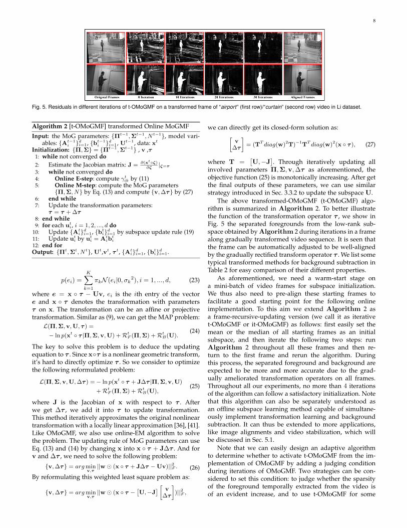
Fig. 5. Residuals in different iterations of t-OMoGMF on a transformed frame of “airport” (first row)/“curtain” (second row) video in Li dataset.

Algorithm 2 [t-OMoGMF] transformed Online MoGMF

Input: the MoG parameters: Πt−1,Σt−1, N t−1, model vari-ables: At−1

i di=1, bt−1i di=1, Ut−1, data: xt

Initialization: Π,Σ = Πt−1,Σt−1 , v ,τ1: while not converged do2: Estimate the Jacobian matrix: J = ∂(xtζ)

∂ζ|ζ=τ

3: while not converged do4: Online E-step: compute γtik by (11)5: Online M-step: compute the MoG parameters

Π,Σ, N by Eq. (13) and compute v,∆τ by (27)6: end while7: Update the transformation parameters:

τ = τ + ∆τ8: end while9: for each uti , i = 1, 2, ..., d do

10: Update Atidi=1, btidi=1 by subspace update rule (19)

11: Update uti by uti = Atibti

12: end forOutput: Πt,Σt, N t, Ut,vt, τ t, At

idi=1, btidi=1.

p(ei) =K∑k=1

πkN (ei|0, σk2), i = 1, ..., d, (23)

where e = x τ − Uv, ei is the ith entry of the vectore and x τ denotes the transformation with parametersτ on x. The transformation can be an affine or projectivetransformation. Similar as (9), we can get the MAP problem:L(Π,Σ,v,U, τ ) =

− ln p(xt τ |Π,Σ,v,U) +RtF (Π,Σ) +RtB(U).(24)

The key to solve this problem is to deduce the updatingequation to τ . Since xτ is a nonlinear geometric transform,it’s hard to directly optimize τ . So we consider to optimizethe following reformulated problem:

L(Π,Σ,v,U,∆τ ) =− ln p(xt τ + J∆τ |Π,Σ,v,U)

+RtF (Π,Σ) +RtB(U),(25)

where J is the Jacobian of x with respect to τ . Afterwe get ∆τ , we add it into τ to update transformation.This method iteratively approximates the original nonlineartransformation with a locally linear approximation [36], [41].Like OMoGMF, we also use online-EM algorithm to solvethe problem. The updating rule of MoG parameters can useEq. (13) and (14) by changing x into x τ + J∆τ . And forv and ∆τ , we need to solve the following problem:

v,∆τ = argminv,τ||w (x τ + J∆τ −Uv)||2F . (26)

By reformulating this weighted least square problem as:

v,∆τ = argminv,τ||w (x τ −

[U,−J

] [ v∆τ

])||2F ,

we can directly get its closed-form solution as:[v

∆τ

]= (TT diag(w)2T)−1TT diag(w)2(x τ ), (27)

where T =[U,−J

]. Through iteratively updating all

involved parameters Π,Σ,v,∆τ as aforementioned, theobjective function (25) is monotonically increasing. After getthe final outputs of these parameters, we can use similarstrategy introduced in Sec. 3.3.2 to update the subspace U.

The above transformed-OMoGMF (t-OMoGMF) algo-rithm is summarized in Algorithm 2. To better illustratethe function of the transformation operator τ , we show inFig. 5 the separated foregrounds from the low-rank sub-space obtained by Algorithm 2 during iterations in a framealong gradually transformed video sequence. It is seen thatthe frame can be automatically adjusted to be well-alignedby the gradually rectified transform operator τ . We list sometypical transformed methods for background subtraction inTable 2 for easy comparison of their different properties.

As aforementioned, we need a warm-start stage ona mini-batch of video frames for subspace initialization.We thus also need to pre-align these starting frames tofacilitate a good starting point for the following onlineimplementation. To this aim we extend Algorithm 2 asa frame-recursive-updating version (we call it as iterativet-OMoGMF or it-OMoGMF) as follows: first easily set themean or the median of all starting frames as an initialsubspace, and then iterate the following two steps: runAlgorithm 2 throughout all these frames and then re-turn to the first frame and rerun the algorithm. Duringthis process, the separated foreground and background areexpected to be more and more accurate due to the grad-ually ameliorated transformation operators on all frames.Throughout all our experiments, no more than 4 iterationsof the algorithm can follow a satisfactory initialization. Notethat this algorithm can also be separately understood asan offline subspace learning method capable of simultane-ously implement transformation learning and backgroundsubtraction. It can thus be extended to more applications,like image alignments and video stabilization, which willbe discussed in Sec. 5.1.

Note that we can easily design an adaptive algorithmto determine whether to activate t-OMoGMF from the im-plementation of OMoGMF by adding a judging conditionduring iterations of OMoGMF. Two strategies can be con-sidered to set this condition: to judge whether the sparsityof the foreground temporally extracted from the video isof an evident increase, and to use t-OMoGMF for some

9

TABLE 2Model comparison of typical transformed background subtraction methods

Method Foreground/BackgroundDecomposition Objective Function Constraint/Basic Assumption Implementation Scheme

RASL [36] τ X = L + S minL,S,τ ||L||∗ + λ||S||1 No OfflineEbadi et al. [38] τ X = L + S + E minL,S,τ ||E||2F + λ||S||1 rank(L) ≤ k OfflineincPCP TI [40] xt = h ∗ (α l) + s + e minl,s,h,α ||e||2F + λ1||s||1 + λ2||h||1 rank(Lt) ≤ k Onlinet-GRASTA [41] τ xt = Uv + s minv ||s||1 UT U = I Online: Heuristically update U

t-OMoGMF τ xt = Uv + eminΠ,Σ,v,U,τ − ln p(τ xt|Π,Σ,v,U)

+RtF (Π,Σ) +Rt

B(U)ei ∼

∑Kk=1 πkN (e|0, σ2

k) Online: Optimize U

TABLE 3F-measure(%) comparison of all competing methods on all video sequences in Li dataset. Each value is averaged over all foreground-annotated

frames in the corresponding video. The most right column lists the average performance of each competing method over all video sequences. Thebest result in each video sequence is highlighted in bold and the second best is in italic. The methods with bold titles denote the online methods.

Methods dataairp. boot. shop. lobb. esca. curt. camp. wate. foun. Average

RPCA [12] 71.11 67.67 72.79 78.12 64.09 81.65 44.56 65.56 72.39 68.66GODEC [15] 62.69 58.39 70.71 73.29 57.42 59.84 43.71 48.79 66.01 60.09RegL1 [24] 65.63 62.46 71.97 75.27 60.95 62.69 44.42 57.86 73.17 63.82PRMF [13] 65.87 62.29 71.99 75.32 60.20 65.17 44.04 61.95 72.98 64.42

OPRMF [13] 66.17 61.82 71.95 73.99 60.12 70.86 42.89 61.89 71.80 64.61GRASTA [17] 61.87 58.07 71.47 60.98 57.26 68.20 44.53 75.88 69.23 63.05incPCP [34] 59.84 62.47 71.28 75.83 45.59 61.10 44.55 74.94 70.49 62.90

PracReProCS [33] 70.01 63.71 71.61 61.89 56.08 77.74 42.28 87.53 62.76 65.96OMoGMF 74.08 59.87 71.80 78.01 61.42 86.08 44.48 87.34 71.78 70.54

DECOLOR [14] 63.98 59.97 65.37 68.93 75.93 89.56 77.14 64.03 86.76 72.41GOSUS [18] 65.80 61.95 72.12 80.97 86.27 68.26 51.30 84.37 73.15 71.35

OMoGMF+TV 77.20 61.17 72.43 83.47 66.37 92.54 65.88 93.14 82.53 77.19

(a) Original frames (b) Transformed framesFig. 6. Typical frames in 9 video sequences of the original and trans-formed Li dataset.

equidistant frames to detect whether the calculated transfor-mation operator is an approximate identity mapping. Bothstrategies can be easily formulated. Such amelioration tendsto facilitate the proposed strategy to better adapt real scenes.

4 EXPERIMENTS

In this section we depict the performance of the pro-posed methods on videos with static and dynamic back-grounds, respectively. All experiments were implementedon a personal computer with i7 CPU and 32G RAM.

4.1 On videos without camera jitterDataset. In this experiments we employ the Li dataset3,

including 9 video sequences, each pictured under a fixedsurvivance camera to certain scene. Typical frames in thesevideos are depicted in Fig. 6(a). These video sequencesrange over a wide range of background cases, like staticbackground (e.g., airport, bootstrap, shoppingmall), illumina-tion changes (e.g., lobby), dynamic background indoors (e.g.,

3. http://perception.i2r.a-star.edu.sg/bk model/bk index.html

escalator, curtain) and dynamic background outdoors (e.g.,campus, watersurface, fountain)4. For each video, we choose200 frames for training. Each sequence contains multipleframes with pre-annotated groundtruth foregrounds andthey are also added into the training data for evaluating theaccuracy of foreground region by each competing method.

Comparison methods. We adopted a series of typicaloffline and online state-of-the-art background subtractionmethods for experiment comparison. The utilized offlinemethods include: PRCA5, GODEC6, RegL17, PRMF8, DE-COLOR9, and online methods include: OPRMF8, GOSUS10,GRASTA11, incPCP12, PracReProCS13. Beyond other com-peting methods, DECOLOR, GOSUS and OMoGMF+TVspecifically consider the spatial smoothness over the fore-ground region, making them always get higher accuracy incapturing foreground objects.

Experiments setup. For RPCA, RegL1, PRMF, OPRMF,DECOLOR, GRASTA,incPCP and PracReProCS, we usethe default parameter settings in the original codes. ForGODEC, we set the sparse parameter by using the resultof RPCA. For GOSUS, we set λ using cross-validation, andset others by default settings. For all low-rank methods,we empirically set a proper rank for each video, and thisrank parameter is set the same for all competing methods in

4. We use the first three/four letters of each sequence name as itsabbreviation in later experiments.

5. http://perception.csl.illinois.edu/matrix-rank/home.html6. https://tianyizhou.wordpress.com/7. https://sites.google.com/site/yinqiangzheng/8. http://winsty.net/prmf.html9. http://bioinformatics.ust.hk/decolor/decolor.html10. http://pages.cs.wisc.edu/ jiaxu/projects/gosus/11. http://sites.google.com/site/hejunzz/grasta12. https://sites.google.com/a/istec.net/prodrig/Home/en/pubs/incpcp13. http://www.ece.iastate.edu/%7Ehanguo/PracReProCS.html

10

Original frames Ground truth RPCA GODEC RegL1 PRMF OPRMF GRASTA incPCP PracReProCS OMoGMF DECOLOR GOSUS OMoGMF+TV

Fig. 7. From left to right: typical frames from curtain and watersurface sequences, groundtruth foreground objects, foregrounds detected by allcompeting methods.

TABLE 4FPS of online competing methods on three videos, each with 200

frames while with different frame size, in Li dataset.

Video esca. airp. shop.Frame Size 130× 160 144× 176 256× 320

OPRMF [13] 0.5 0.4 0.1PracReProCS [33] 1.5 1.2 0.2

GOSUS [18] 3.8 2.7 0.6OMoGMF+TV 18.5 14.8 3.5

OMoGMF 99.6 63.0 5.2GRASTA [17] 166.9 123.9 28.7incPCP [34] 274.5 220.8 85.2

GRASTA&1%SS 303.2 246.7 65.5OMoGMF&1%SS 332.0 263.6 104.7

each video. For all online competing methods, we randomlychoose some frames and use robust batch method and PCAto initialize the subspace. We use GMM on the residualsto initialize the MoG parameters for OMoGMF, and thenumber of MoG components is set as 3 throughout allour experiments. The foreground obtained by the proposedmethods are taken as the MoG noise component with thelargest variance. More details on parameter setting in ourexperiments are introduced in SM.

Performance Evaluation. The F-measure is utilized asthe quantitative metric for performance evaluation. TheF-measure is calculated as follows:

F-measure = 2× precision · recallprecision+ recall

,

where precision =|Sf

⋂Sgt|

|Sf | and recall =|Sf

⋂Sgt|

|Sgt| , Sfand Sgt denote the support sets of the foreground calculatedfrom the method and the ground truth one, respectively. F-measure is close to the smaller one of precision and recall.Besides, we choose the value of the threshold which canmake F-measure largest for each competing method. Thelarger the F-measure, the more accurate the foreground objectis detected by the method.

Foreground detection accuracy comparison. Table 3lists the average F-measure over all foreground-annotatedframes calculated from all competing methods on all videosequences in Li dataset. It is seen that in average OMoGMFhas an evidently better performance than other competingmethods without considering spatial smoothness of videos,and so does OMoGMF+TV than all. This superiority of theOMoGMF and OMoGMF+TV methods can also be observedfrom Fig. 7, which shows the detected foregrounds ontypical frames of tested videos by all competing methods. It

is easy to see that the detected foregrounds by the proposedmethods are closer to the groundtruth ones, which conductsits larger F-measures in experiments.

The advantage of the proposed methods can be easilyexplained by their flexible noise fitting capability along time.Specifically, while other competing methods only assumea fixed noise distribution throughout a video sequenceand separate one layer of foreground from the video, ourmethods can adapt a specific MoG noise for each videoframe, and thus can more elaborately recover multiple lay-ers of foreground knowledge. Especially, the extracted noisecomponent with largest variance generally dominates theforeground object, while other noise components character-ize smaller variations accompanied besides the object. E.g.,for lobby and campus sequences, except that the noise com-ponent with largest variance properly delivers the movingobjects in the video, the other two components finely cap-ture the shadow along the object + weak camera noise andleaves shaking variance + weak camera noise, respectively,as clearly depicted in Fig. 1. Due to such ability of clearingaway trivial noise variations, our methods then rationallyattain better foreground object extraction performance14.

Effects on videos with background changes andmissing entries. Beyond offline methods, which are rela-tively sensitive to background changes, the proposed onlinemethod can finely adapt sudden background changes. Fig.8(a) shows the background subtraction result by OMoGMFfor frames in lobby sequence with a illumination change. Itis seen that OMoGMF can gradually adapt a proper back-ground after multiple frames’ self-ameliorating. Further-more, OMoGMF can also be used to deal with videos withmissing entries by adopting the sub-sampling technique.Fig. 8(b) shows background subtraction result on airportsequence, with 85% of its entries missed under a randomsubspace initialization. It is easy to see that our onlinemethod can gradually recover the proper background.

Speed Evaluations. In our experiments, just as substan-tiated by previous research, all offline competing methodsare significantly slower than online methods, which is es-pecially more evident for those videos with relatively moreframes and larger sizes. So here we only compare the speedof the online competing methods. The FPS (frames persecond) is utilized as the comparison metric. Table 4 showsthe FPS of all online competing methods on three videoswith different frame sizes. Though the FPS of OMoGMF

14. More demos on depicting such noise fitting capability of the pro-posed methods are shown in http://gr.xjtu.edu.cn/web/dymeng/7.

11

TABLE 5F-measure(%) and FPS of OMoGMF and GRASTA under different sub-sampling rates on 3 videos, each with 1000 frames and different framesize, in Li dataset. The average is computed on the results of both methods on all 9 videos of Li dataset. Detailed results are reported in SM.

Sub-Sampling rate 1% 10% 30% 50% 100%Dataset frame size method F-M FPS F-M FPS F-M FPS F-M FPS F-M FPS

esca. 130× 160 OMoGMF 61.01 332.0 61.19 265.9 61.26 172.3 61.28 137.5 61.20 99.6GRASTA 45.81 303.2 58.97 264.6 58.70 212.8 58.21 180.2 57.32 166.9

airp. 144× 176 OMoGMF 71.31 263.6 72.30 181.6 72.38 115.7 72.42 91.7 72.41 63.0GRASTA 63.12 246.7 64.03 209.6 63.25 167.6 62.56 141.3 61.94 123.9

shop. 256× 320 OMoGMF 69.42 104.7 69.46 40.2 69.47 16.1 69.48 10.2 69.50 5.2GRASTA 65.35 65.5 71.00 56.7 71.43 44.2 71.51 37.1 71.46 28.7

AverageOMoGMF 69.82 273.4 70.30 189.4 70.33 114.2 70.35 86.1 70.34 57.6GRASTA 57.16 244.0 64.30 213.9 65.16 171.1 64.58 145.7 63.07 128.7

TABLE 6F-measure(%) of different competing methods on Li dataset added with artificial transformations.

Methods dataairp. boot. shop. lobb. esca. curt. camp. wate. foun. Average

RPCA [12] 58.53 59.10 53.67 19.48 44.87 62.04 32.81 51.40 38.49 46.71GRASTA [17] 52.96 50.38 41.38 9.19 32.85 58.54 24.23 44.22 19.93 37.08

OMoGMF 51.97 49.35 39.71 9.36 28.19 66.77 21.05 74.35 19.90 40.07RASL [36] 68.94 66.46 76.42 61.17 72.53 69.91 58.87 30.18 71.17 63.96

t-GRASTA [41] 69.23 56.91 46.57 56.35 64.26 83.01 51.15 88.34 72.89 65.41t-OMoGMF 75.21 65.08 74.92 65.57 66.16 89.62 53.65 89.79 79.41 73.27

t=400 t=440 t=480 t=520

(a) Video sequence with illumination change

t=1 t=30 t=80 t=200

(b) Sequence with missing entries

Fig. 8. Performance of OMoGMF on video sequences with (a) suddenillumination change and (b) missing entries. From upper to lower: (a)Original video frames, extracted backgrounds and residuals; (b) Originalvideo frames, 15% subsampling frames, extracted backgrounds.

is not the highest, the OMoGMF can achieve the real-timeprocessing in most case. Sub-sampling technique can be eas-ily used into GRASTA and OMoGMF to further acceleratetheir computation. We also show the FPS of GRASTA andOMoGMF with 1% subsampling rate in this table. Underlow subsampling rate, OMoGMF can attain more than 200

Fig. 9. From upper to lower: original frames in the shoppingmall video,backgrounds and residuals (brightening 0.5 gray scales for all pixels forbetter visualization) obtained by OMoGMF with 1% sub-sampling rate.

FPS on average for executing these videos while also keep ahigh F-measure so that it can meet the real-time requirementin practice. To better clarify this point, Table 5 shows theperformance of OMoGMF and GRASTA under differentsub-sampling rates on 3 videos with different sizes, eachwith 1000 frames. It can be seen that as the sub-samplingrate decreasing, OMoGMF is gradually more accurate andfaster than GRASTA in all videos. Specifically, in 5 of 9videos, GRASTA has an evident drop in F-measure15. Com-paratively, even under 1% sub-sampling rate, the F-measureobtained by OMoGMF is only very slightly decreased thanthat on the original videos. As shown in Fig. 9, even undersuch a low sub-sampling rate, OMoGMF can still finelycapture foreground and background of original videos.

15. On multiple videos, the GRASTA method has a surprising in-crease on F-measure under 1% sub-sampling rate than the method onthe original videos. This might be due to the fact that the sub-samplingtechnique helps alleviate the negative influence of the complex noiseconfigurations, especially in the videos with dynamic backgrounds.

12

TABLE 7F-measure(%) comparison of transformed methods on real data with

camera jitter

Methods databadm. boul. side. traf. Average

RASL [36] 72.86 73.62 47.16 67.77 65.35t-GRASTA [41] 68.99 72.62 56.20 67.28 66.27

t-OMoGMF 69.97 69.78 59.20 83.44 70.60

Fig. 10. From upper to lower: original frames in airport video; alignedframes, backgrounds and foregrounds obtained by t-OMoGMF.

4.2 On videos with camera jitter

We then test the t-OMoGMF method on videos withcamera jitter. The comparison methods include state-of-the-art subspace alignment methods: RASL16 and t-GRASTA17.

Synthetic data: As [41], we design 9 synthetic jittervideo sequences from Li dataset with background trans-formations. 400 adjacent frames are selected from eachvideo, and each frame is randomly rotated with an angle in[−5, 5] and translated in both axes with a range in [-5,5],respectively. Typical frames of all videos so generated areshown in Fig. 6(b). We randomly choose 30 frames for eachvideo for subspace initialization. The rank is set as 3 for allcompeting methods. Table 6 shows the F-measure obtainedby t-OMoGMF, RASL and t-GRASTA in all test videos. Be-sides, the results of PRCA, GRASTA and OMoGMF, whichdo not consider frame transformations, are also comparedto show the function of the involvement of this transforma-tion operator. The superiority of t-OMoGMF can be easilyobserved: It performs the best/the second best in 5/4 out of9 videos, and on average it performs more than 10% betterthan other methods. For better observation, Fig. 10 showsthe result of t-OMoGMF on multiple frames of transformedairport sequence. It is easy to see that t-OMoGMF canwell align video frames, which naturally leads to its betterforeground/background separation. About computationalspeed, our method can run more than 5 times faster thanRASL and slightly faster than t-GRASTA on average.

Real data: In this experiment, we use a set of real-world videos for assessing the performance of the pro-posed t-OMoGMF method. The dataset contains 4 video se-quences18: badminton, boulevard, sidewalk and traffic, all withevident camera jitters. As set in synthetic experiments, weset subspace rank as 3 for all competing methods, and ran-domly choose 30 frames from each video to train the initial

16. http://perception.csl.uiuc.edu/matrix-rank/rasl.html17. https://sites.google.com/site/hejunzz/t-grasta18. http://www.changedetection.net

Fig. 11. From upper to lower: original frames in sidewalk video; resid-uals on unaligned frames; frames aligned by t-OMoGMF; backgroundsobtained by t-OMoGMF; foregrounds detected by t-OMoGMF.

subspace and model parameters. In all our experiments, t-OMoGMF can properly align all video frames, and simulta-neously appropriately separate background and foregroundfrom the jitter videos19. Some typical frames are shown inFig. 11. Furthermore, Table 7 quantitatively compares theperformance of all competing methods in terms of the F-measure on these real videos, and the superiority of theproposed t-OMoGMF can still be observed on average. Be-sides, while RASL and GRASTA may also detect foregroundobjects from videos, our method can always more clearlyrecover the background and clean up various unexpectednoise variations from the video, as clearly depicted in Fig. 2.

5 CONCLUSION AND DISCUSSION

5.1 Extension to other tasksAs aforementioned in Section 3.6, the proposed it-

OMoGMF method can be easily extended to image align-ment and video stabilization tasks. Here we provide somepreliminary tests to illuminate this point.

Two datasets were adopted in this experiment: one is the“dummy” imageset [36], a synthetic face dataset containing100 misaligned faces with block occlusions and illuminationvariations; the other is the “Gore” video sequence [36], a140-frame video of Al Gore talking, obtained by applying aface detector to each frame independently. Due to inherentimprecision of the detector, there is significant jitters fromframe to frame [36]. As previous state-of-the-art methodsimplemented on these datasets, the proposed it-OMoGMFmethod can also finely align all of the images/frames intwo datasets, as clearly demonstrated in Fig. 12 and 13,respectively. Yet beyond other methods, it-OMoGMF canmore elaborately separate multiple layers of noises fromdata, which always have certain physical meanings. E.g.,the noise components with largest variance in two datasetsclearly represent the occlusion part for “dummy” imagesand expression variations for ”Gore” video, respectively.

5.2 Concluding remarksIn this paper, we have proposed a new online sub-

space learning method aiming to make background sub-traction available in practical videos both in speed and

19. Please see more demos in http://gr.xjtu.edu.cn/web/dymeng/7.

13

Fig. 12. From upper to lower: original images in “dummy” set; imagesaligned by it-OMoGMF; images recovered by it-OMoGMF; occlusionsand small variations detected by it-OMoGMF. The last column is aver-aged over all images.

accuracy. On one hand, the computational speed of thenew method reaches the real-time requirement for videoprocessing (more than 25 FPS), and on the other hand,the method can adaptively fit real-time dynamic varia-tions in both foreground and background of videos. Inparticular, through specifically learning a foreground dis-tribution and a background subspace regularized by thepreviously learned knowledge for each video frame, themethod can properly deliver variations of video foregroundand background along the video sequence. Through furtherinvolving the variables to encode affine transformation op-erators on each video frame, the method can further adaptthe background transformations, like rotations, transforma-tions, scalings and distortions, generally existed in practicalvideos. Furthermore, by virtue of the sub-sampling and TV-norm regularization technique amelioration, the efficiencyand accuracy of the proposed method can be further im-proved. The superiority of the proposed method has beenextensively substantiated, as compared with other state-of-the-art online and offline methods along this research line,by experiments on synthetic and real-world videos.

5.3 Future work

In our future investigations, we will try to embed thesub-sampling technique into t-OMoGMF and it-OMoGMFto further improve their speed and apply our methods tolarger real-time video streaming. Also, more video process-ing tasks are worthy to be intrinsically integrated with theproposed methods, especially to make full use of the real-timely detected foreground objects by the proposed meth-ods. Recently, there are multiple literatures discussing theparameter selection issue, like the subspace rank [25] andthe number of noise components [26], in subspace learning.We’ll also consider to combine these techniques into ourmethod to make its parameter selection more proper andautomatic. Besides, we will try to extend our method toother computer vision and image processing applications.

REFERENCES

[1] C. Beleznai, B. Fruhstuck, and H. Bischof, “Multiple object trackingusing local PCA,” in Pattern Recognition, 2006. ICPR 2006. 18thInternational Conference on, vol. 3. IEEE, 2006, pp. 79–82.

Fig. 13. From upper to lower: original frames from “Gore” video; framesaligned by it-OMoGMF; frames recovered by it-OMoGMF; expressionchanges and small variations detected by it-OMoGMF. The last columnis averaged over all frames.

[2] S.-C. S. Cheung and C. Kamath, “Robust background subtractionwith foreground validation for urban traffic video,” Eurasip Journalon applied signal processing, vol. 2005, pp. 2330–2340, 2005.

[3] A. W. Senior, Y. Tian, and M. Lu, “Interactive motion analysis forvideo surveillance and long term scene monitoring,” in ComputerVision–ACCV 2010 Workshops. Springer, 2011, pp. 164–174.

[4] “A novel tensor robust pca.”[5] B. Lee and M. Hedley, “Background estimation for video surveil-

lance,” IVCNZ02, pp. 315–320, 2002.[6] N. J. McFarlane and C. P. Schofield, “Segmentation and tracking

of piglets in images,” Machine vision and applications, vol. 8, no. 3,pp. 187–193, 1995.

[7] J. Zheng, Y. Wang, N. Nihan, and M. Hallenbeck, “Extractingroadway background image: Mode-based approach,” Transporta-tion Research Record: Journal of the Transportation Research Board, no.1944, pp. 82–88, 2006.

[8] C. Stauffer and W. E. L. Grimson, “Adaptive background mixturemodels for real-time tracking,” in Computer Vision and PatternRecognition, 1999. IEEE Computer Society Conference on., vol. 2.IEEE, 1999.

[9] M. S. Allili, N. Bouguila, and D. Ziou, “A robust video foregroundsegmentation by using generalized gaussian mixture modeling,”in Computer and Robot Vision, 2007. CRV’07. Fourth Canadian Con-ference on. IEEE, 2007, pp. 503–509.

[10] T. Bouwmans and E. H. Zahzah, “Robust PCA via principalcomponent pursuit: A review for a comparative evaluation invideo surveillance,” Computer Vision and Image Understanding, vol.122, pp. 22–34, 2014.

[11] T. Bouwmans, A. Sobral, S. Javed, S. K. Jung, and E.-H. Za-hzah, “Decomposition into low-rank plus additive matrices forbackground/foreground separation: A review for a comparativeevaluation with a large-scale dataset,” Computer Science Review,2016.

[12] E. J. Candes, X. Li, Y. Ma, and J. Wright, “Robust principalcomponent analysis?” Journal of the ACM (JACM), vol. 58, no. 3,p. 11, 2011.

[13] N. Wang, T. Yao, J. Wang, and D.-Y. Yeung, “A probabilistic ap-proach to robust matrix factorization,” in Computer Vision–ECCV2012. Springer, 2012, pp. 126–139.

[14] X. Zhou, C. Yang, and W. Yu, “Moving object detection by detect-ing contiguous outliers in the low-rank representation,” PatternAnalysis and Machine Intelligence, IEEE Transactions on, vol. 35, no. 3,pp. 597–610, 2013.

[15] T. Zhou and D. Tao, “GODEC: Randomized low-rank & sparsematrix decomposition in noisy case,” 2011.

[16] D. Meng and F. De la Torre, “Robust matrix factorization withunknown noise,” in IEEE International Conference on ComputerVision, 2013, pp. 1337–1344.

[17] J. He, L. Balzano, and A. Szlam, “Incremental gradient on theGrassmannian for online foreground and background separationin subsampled video,” in Computer Vision and Pattern Recognition(CVPR), 2012 IEEE Conference on. IEEE, 2012, pp. 1568–1575.

[18] J. Xu, V. K. Ithapu, L. Mukherjee, J. M. Rehg, and V. Singh,“GOSUS: Grassmannian online subspace updates with structured-sparsity,” in Computer Vision (ICCV), 2013 IEEE International Con-ference on. IEEE, 2013, pp. 3376–3383.

14

[19] F. De La Torre and M. J. Black, “A framework for robust subspacelearning,” International Journal of Computer Vision, vol. 54, no. 1-3,pp. 117–142, 2003.

[20] K. R. Gabriel and S. Zamir, “Lower rank approximation of matricesby least squares with any choice of weights,” Technometrics, vol. 21,no. 4, pp. 489–498, 1979.

[21] N. Srebro, T. Jaakkola et al., “Weighted low-rank approximations,”in ICML, vol. 3, 2003, pp. 720–727.

[22] T. Okatani and K. Deguchi, “On the Wiberg algorithm for matrixfactorization in the presence of missing components,” InternationalJournal of Computer Vision, vol. 72, no. 3, pp. 329–337, 2007.

[23] A. Eriksson and A. Van Den Hengel, “Efficient computation ofrobust low-rank matrix approximations in the presence of missingdata using the L1 norm,” in Proceedings of IEEE Conference onComputer Vision and Pattern Recognition, 2010, pp. 771–778.

[24] Y. Zheng, G. Liu, S. Sugimoto, S. Yan, and M. Okutomi, “Practicallow-rank matrix approximation under robust L1-norm,” in Com-puter Vision and Pattern Recognition (CVPR), 2012 IEEE Conferenceon. IEEE, 2012, pp. 1410–1417.

[25] Q. Zhao, D. Meng, Z. Xu, W. Zuo, and L. Zhang, “Robust principalcomponent analysis with complex noise,” in Proceedings of the 31stInternational Conference on Machine Learning (ICML-14), 2014, pp.55–63.

[26] X. Cao, Y. Chen, Q. Zhao, D. Meng, Y. Wang, D. Wang, andZ. Xu, “Low-rank matrix factorization under general mixture noisedistributions,” in International Conference on Computer Vision, 2015.

[27] T. M. Nguyen and Q. J. Wu, “Robust student’s-t mixture modelwith spatial constraints and its application in medical imagesegmentation,” Medical Imaging, IEEE Transactions on, vol. 31, no. 1,pp. 103–116, 2012.

[28] T. S. Haines and T. Xiang, “Background subtraction with Dirichletprocesses,” in Computer Vision–ECCV 2012. Springer, 2012, pp.99–113.

[29] M. Braham and M. Van Droogenbroeck, “Deep background sub-traction with scene-specific convolutional neural networks,” inSystems, Signals and Image Processing (IWSSIP), 2016 InternationalConference on. IEEE, 2016, pp. 1–4.

[30] M. Babaee, D. T. Dinh, and G. Rigoll, “A deep convolu-tional neural network for background subtraction,” arXiv preprintarXiv:1702.01731, 2017.

[31] S. Javed, A. Sobral, T. Bouwmans, and S. K. Jung, “OR-PCA withdynamic feature selection for robust background subtraction,” inProceedings of the 30th Annual ACM Symposium on Applied Comput-ing. ACM, 2015, pp. 86–91.

[32] S. Javed, S. Ho Oh, A. Sobral, T. Bouwmans, and S. Ki Jung, “Back-ground subtraction via superpixel-based online matrix decompo-sition with structured foreground constraints,” in Proceedings of theIEEE International Conference on Computer Vision Workshops, 2015,pp. 90–98.

[33] H. Guo, C. Qiu, and N. Vaswani, “An online algorithm for sep-arating sparse and low-dimensional signal sequences from theirsum,” IEEE Transactions on Signal Processing, vol. 62, no. 16, pp.4284–4297, 2014.

[34] P. Rodriguez and B. Wohlberg, “Incremental principal componentpursuit for video background modeling,” Journal of MathematicalImaging and Vision, vol. 55, no. 1, pp. 1–18, 2016.

[35] ——, “A MATLAB implementation of a fast incremental principalcomponent pursuit algorithm for video background modeling,”in Image Processing (ICIP), 2014 IEEE International Conference on.IEEE, 2014, pp. 3414–3416.

[36] Y. Peng, A. Ganesh, J. Wright, W. Xu, and Y. Ma, “RASL: Robustalignment by sparse and low-rank decomposition for linearlycorrelated images,” Pattern Analysis and Machine Intelligence, IEEETransactions on, vol. 34, no. 11, pp. 2233–2246, 2012.

[37] S. E. Ebadi and E. Izquierdo, “Approximated RPCA for fast andefficient recovery of corrupted and linearly correlated images andvideo frames,” in Systems, Signals and Image Processing (IWSSIP),2015 International Conference on. IEEE, 2015, pp. 49–52.

[38] S. E. Ebadi, V. G. Ones, and E. Izquierdo, “Efficient backgroundsubtraction with low-rank and sparse matrix decomposition,”in Image Processing (ICIP), 2015 IEEE International Conference on.IEEE, 2015, pp. 4863–4867.

[39] ——, “Dynamic tree-structured sparse RPCA via column subsetselection for background modeling and foreground detection,”in Image Processing (ICIP), 2016 IEEE International Conference on.IEEE, 2016, pp. 3972–3976.

[40] P. Rodrıguez and B. Wohlberg, “Translational and rotational jit-ter invariant incremental principal component pursuit for videobackground modeling,” in Image Processing (ICIP), 2015 IEEE In-ternational Conference on. IEEE, 2015, pp. 537–541.

[41] J. He, D. Zhang, L. Balzano, and T. Tao, “Iterative Grassmannianoptimization for robust image alignment,” Image and Vision Com-puting, vol. 32, no. 10, pp. 800–813, 2014.

[42] A. P. Dempster, N. M. Laird, and D. B. Rubin, “Maximum likeli-hood from incomplete data via the EM algorithm,” Journal of theroyal statistical society. Series B (methodological), pp. 1–38, 1977.

[43] C. M. Bishop, Pattern recognition and machine learning. springer,2006.

[44] E. J. Candes and B. Recht, “Exact matrix completion via convexoptimization,” Foundations of Computational mathematics, vol. 9,no. 6, pp. 717–772, 2009.

[45] N. Wang and D.-Y. Yeung, “Bayesian robust matrix factorizationfor image and video processing,” in Computer Vision (ICCV), 2013IEEE International Conference on. IEEE, 2013, pp. 1785–1792.

[46] T.-F. Su, Y.-L. Chen, and S.-H. Lai, “Over-segmentation basedbackground modeling and foreground detection with shadowremoval by using hierarchical MRFs,” in Computer Vision–ACCV2010. Springer, 2011, pp. 535–546.

[47] X. Cao, L. Yang, and X. Guo, “Total variation regularized RPCA forirregularly moving object detection under dynamic background,”2015.

[48] J. Huang, T. Zhang, and D. Metaxas, “Learning with structuredsparsity,” The Journal of Machine Learning Research, vol. 12, pp.3371–3412, 2011.

[49] J. Wang, Q. Li, S. Yang, W. Fan, P. Wonka, and J. Ye, “A highlyscalable parallel algorithm for isotropic total variation models,” inProceedings of the 31st International Conference on Machine Learning(ICML-14), 2014, pp. 235–243.

[50] S. Yang, J. Wang, W. Fan, X. Zhang, P. Wonka, and J. Ye, “Anefficient ADMM algorithm for multidimensional anisotropic totalvariation regularization problems,” in Proceedings of the 19th ACMSIGKDD international conference on Knowledge discovery and datamining. ACM, 2013, pp. 641–649.