1

LIQUIDITY AND LIQUIDITY RISK IN THE CORPORATE

BOND MARKET

Gady Jacoby, George Theocharides

and Steven X. Zheng

Seminar PresentationSeoul National University

November 17th, 2008

2

Outline

• Introduction & Related Literature• Contribution• Theoretical Modeling of Liquidity and Liquidity Risk

(LCAPM)• Data• Empirical Methodology• Results• Robustness Tests• Other Tests

3

Introduction

What do we know about asset pricing and liquidity?

• Asset-specific liquidity impacts asset prices [Amihud and Mendelson (1986, 1989), Brennan et al. (1998), Amihud (2002), Chen, Lesmond, and Wei (2007)]

• Market liquidity impacts asset prices as a systematic risk factor [Pastor and Stambaugh (2003), Acharya and Pedersen (2005), Sadka (2006)]

• Commonality in liquidity affects asset prices [Chordia et al. (2000), Hasbrouck and Seppi (2001), Huberman and Halka (2001), and Acharya and Pedersen (2005)]

4

Related Literature

Empirical evidence

• There is ample evidence that liquidity and liquidity risk affect asset prices in the:

- Equity Market[Amihud and Mendelson (1986, 1989), Brennan and Subrahmanyam (1996), Brennan et al. (1998), Chordia, Roll, and Subrahmanyam (2000, 2001), Amihud (2002), Pastor and Stambaugh (2003), Acharya and Pedersen (2005), Lee (2005), Lesmond (2005)], and in the

- Treasury Market[Sarig and Warga (1989), Amihud and Mendelson (1991), Warga (1992), Kamara (1994), Elton and Green (1998), Krishnamurthy (2002), Longstaff (2004)]

5

Related LiteratureEmpirical evidence…

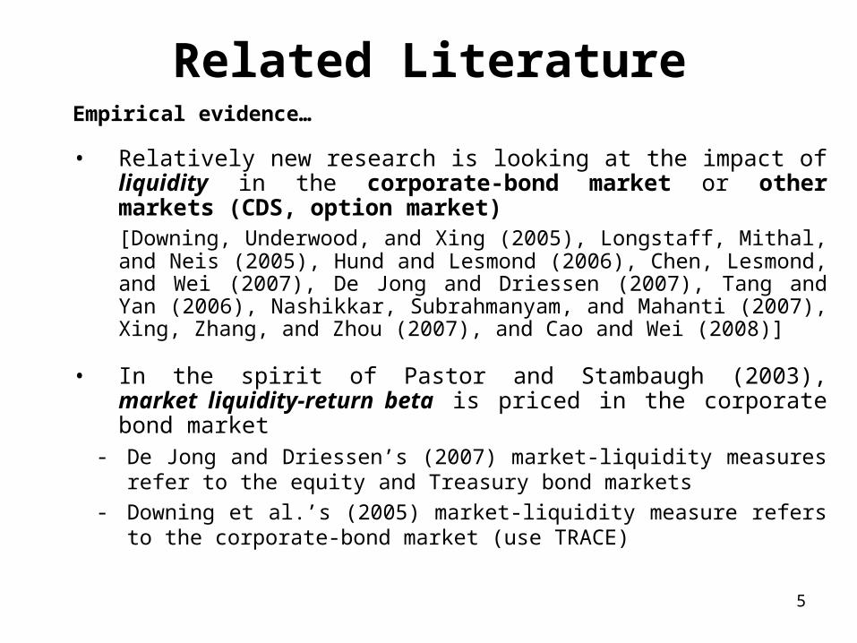
• Relatively new research is looking at the impact of liquidity in the corporate-bond market or other markets (CDS, option market)[Downing, Underwood, and Xing (2005), Longstaff, Mithal, and Neis (2005), Hund and Lesmond (2006), Chen, Lesmond, and Wei (2007), De Jong and Driessen (2007), Tang and Yan (2006), Nashikkar, Subrahmanyam, and Mahanti (2007), Xing, Zhang, and Zhou (2007), and Cao and Wei (2008)]

• In the spirit of Pastor and Stambaugh (2003), market liquidity-return beta is priced in the corporate bond market

- De Jong and Driessen’s (2007) market-liquidity measures refer to the equity and Treasury bond markets

- Downing et al.’s (2005) market-liquidity measure refers to the corporate-bond market (use TRACE)

6

Related LiteratureEmpirical evidence…

• Commonality in liquidity is priced in the corporate bond market- Xing et al. (2007) measure commonality in liquidity with respect to

the corporate-bond markets (use TRACE)

Our Contribution

• The current paper examines the effect of liquidity and liquidity risk, in the context of the Acharya and Pedersen’s (2005) LCAPM, and simultaneously considers the effect of all sources of liquidity risk (arising from the corporate bond, Treasury, and equity markets) on expected or realized bond returns

7

Theoretical Modeling of Liquidity and Liquidity Risk

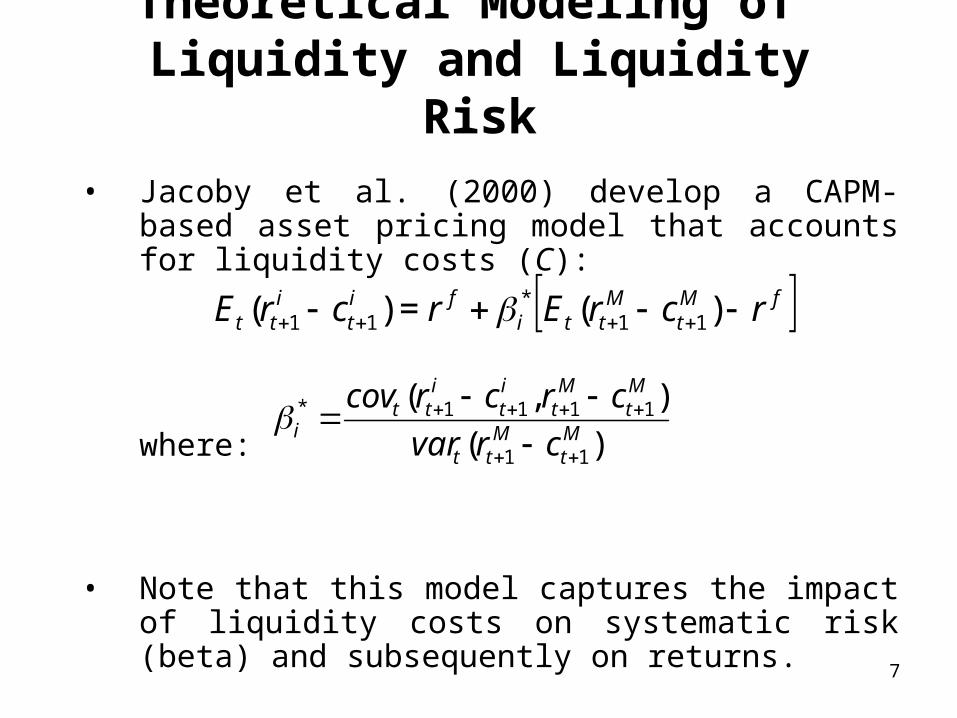
• Jacoby et al. (2000) develop a CAPM-based asset pricing model that accounts for liquidity costs (C):

where:

• Note that this model captures the impact of liquidity costs on systematic risk (beta) and subsequently on returns.

fMt

Mtti

fit

itt rcrErcrE )(=)( 11

*11

)(

),(

11

1111*Mt

Mtt

Mt

Mt

it

itt

i crvar

crcrcov

8

Theoretical Modelling of Liquidity and Liquidity Risk…

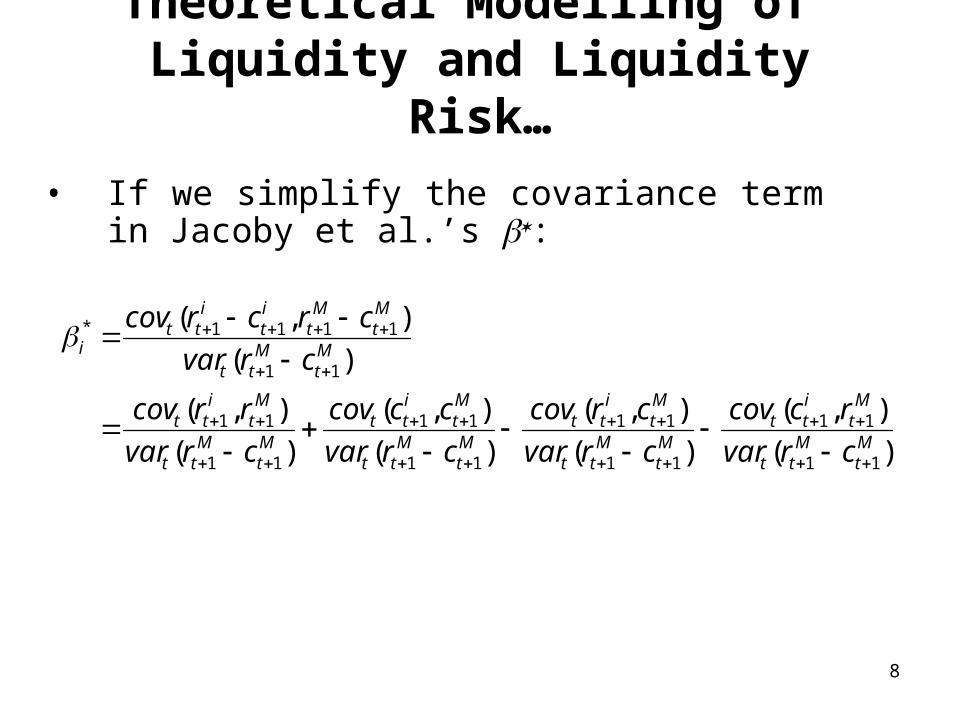
• If we simplify the covariance term in Jacoby et al.’s :

)(

),(

)(

),(

)(

),(

)(

),(

)(

),(

11

11

11

11

11

11

11

11

11

1111*

Mt

Mtt

Mt

itt

Mt

Mtt

Mt

itt

Mt

Mtt

Mt

itt

Mt

Mtt

Mt

itt

Mt

Mtt

Mt

Mt

it

itt

i

crvar

rccov

crvar

crcov

crvar

cccov

crvar

rrcov

crvar

crcrcov

9

Theoretical Modelling of Liquidity and Liquidity Risk…

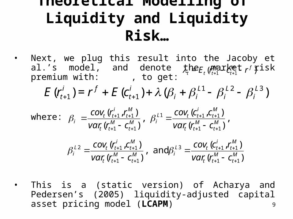
• Next, we plug this result into the Jacoby et al.’s model, and denote the market risk premium with: , to get:

where:

• This is a (static version) of Acharya and Pedersen’s (2005) liquidity-adjusted capital asset pricing model (LCAPM)

)(= 11fM

tM

ttt rcrE

)()(=)( 32111

Li

Li

Lii

it

fit cErrE

,)(

),( ,

)(

),(

11

111

11

11Mt

Mtt

Mt

ittL

iMt

Mtt

Mt

itt

i crvar

cccov

crvar

rrcov

)(

),( and ,

)(

),(

11

113

11

112Mt

Mtt

Mt

ittL

iMt

Mtt

Mt

ittL

i crvar

rccov

crvar

crcov

10

The LCAPM: Intuition

The LCAPM is simple and intuitive. It states that the required return is a function of:

• the asset expected illiquidity cost, , and

• four betas (or covariances) times the market risk premium ().

- The four betas depend on the asset returns and liquidity costs.

- The LCAPM yields three additional betas, regarded as three forms of liquidity risks.

)( 1itcE

11

The LCAPM: Intuition…

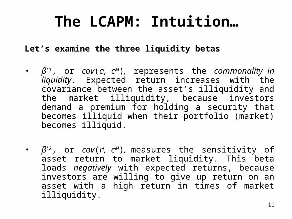
Let’s examine the three liquidity betas

• βL1, or cov(ci, cM), represents the commonality in liquidity. Expected return increases with the covariance between the asset’s illiquidity and the market illiquidity, because investors demand a premium for holding a security that becomes illiquid when their portfolio (market) becomes illiquid.

• βL2, or cov(ri, cM), measures the sensitivity of asset return to market liquidity. This beta loads negatively with expected returns, because investors are willing to give up return on an asset with a high return in times of market illiquidity.

12

The LCAPM: Intuition…

Let’s examine the three liquidity betas…

• βL3, or cov(ci, rM), measures the sensitivity of asset liquidity to market return. This beta also loads negatively with expected returns, because investors are willing to give up return on a security that is liquid in a down market. When the market declines, investors are poor and the ability to easily sell becomes valuable.

• Acharya and Pederson (2005) show that, in general, empirically all four betas can help to explain returns in the U.S. equity market.

13

Data• We test the LCAPM using the newly formed Trade Reporting and Compliance

Engine (TRACE) system.

• TRACE was established by NASD on July 1, 2002, in an effort to increase post-trade transparency for corporate bonds.

• NASD requires from all its members (dealers) to report in a relatively-short period of time all transactions on bonds that are eligible under the TRACE system (according to a press release on February 7th, 2005 found on the NASD's website, by the end of 2004 82% of transactions were reported in five minutes or less).

• Majority of transactions are by retail investors (according to a report on Sept. 30 th, 2004, 65% of corporate bond transactions are of $100,000 or less in size).

• Information reported to TRACE but not yet disseminated includes indicators for whether it's a buy or sell by the customer; inter-dealer trades; whether the broker-dealer reporting the transaction is acting as agent or principal; and the identification of the dealer and the counterparty.

14

• TRACE disseminated trade information in phases:- Phase I (July 1, 2002): Included 550 investment-grade (IG)

bonds with an original issue size of at least $1 billion, as well as 50 low-grade (high yield, HY) bonds.

- Phase IIa (March 3, 2003): the number of bonds under dissemination increased to 4,200 (bonds with an issue size of at least $100 million and an A3/A- rating or higher were added).

- Phase IIb (April, 2003): Another 120 BBB-rated bonds were added.

- Phase III (October 1, 2004): The entire universe of U.S. corporate bonds is included under TRACE.

Data…

15

• Data set utilized in our study covers the period from Jan. 1, 2003, to Dec., 31, 2006. It is merged with FISD to obtain issue/issuer characteristics

• We include callable bonds, but exclude bonds carrying other options

• Cancelled, corrected, commission and outlier trades (obs. that fall in the top/bottom 1% of the sample) are removed. Also, we remove observations with negative spreads, or negative excess bond returns.

• Final dataset consists of 4,577,001 transactions

Data…

16

Panel A: No. of trans. by year Issues/year Issuers/year

N % N N2003-2006 4,577,001 100.0 5,673 1,502

2003 767,041 16.8 2,327 6962004 908,602 19.9 4,061 1,1242005 1,415,186 30.9 5,010 1,4212006 1,486,172 32.5 4,329 1,298

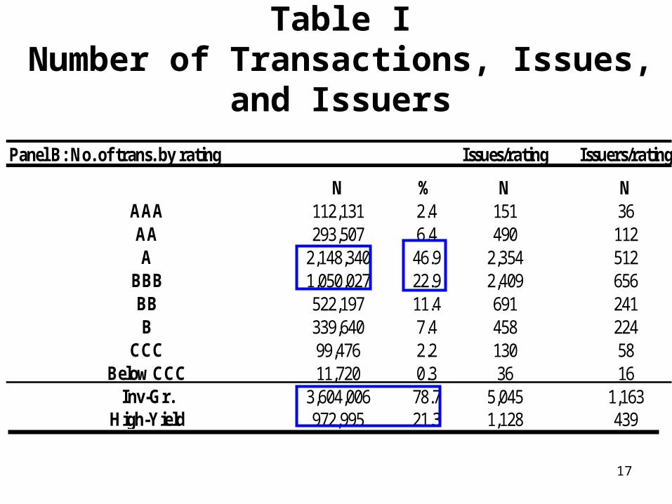
Table INumber of Transactions, Issues, and Issuers

17

Panel B: No. of trans. by rating Issues/rating Issuers/rating

N % N NAAA 112,131 2.4 151 36AA 293,507 6.4 490 112A 2,148,340 46.9 2,354 512

BBB 1,050,027 22.9 2,409 656BB 522,197 11.4 691 241B 339,640 7.4 458 224

CCC 99,476 2.2 130 58Below CCC 11,720 0.3 36 16

Inv-Gr. 3,604,006 78.7 5,045 1,163High-Yield 972,995 21.3 1,128 439

Table INumber of Transactions, Issues, and Issuers

18

Panel C: No. of trans. by industry Issues/industry Issuers/industryN % N N

Industrial 2,625,902 57.4 2,846 822Financial 1,518,512 33.2 1,893 411

Utility 432,587 9.5 1,134 269

Table INumber of Transactions, Issues, and Issuers

19

Panel D: No. of trans. by maturity Issues/maturity Issuers/maturity

N % N NShort (0-7 yrs) 2,850,511 62.3 4,121 1,338

Medium (7-15 yrs) 947,807 20.7 1,403 776Long (15 yrs-30 yrs) 737,897 16.1 1,015 497

V. Long (30 yrs-onwards) 40,786 0.9 148 110

Table INumber of Transactions, Issues, and Issuers

20

Table IIBond Characteristics

Mean Median 25% quantile 75% quantile Max

Issue Size ($million) 250 200 100 300 3,000

Original maturity (years) 14 10 9 15 100

Years to maturity 7.92 4.89 2.31 9.10 100.02

Age (years) 5.53 4.85 2.32 8.15 69.52

Trade size ($K) 440 25 10 200 5000

Daily volume ($K) 1,874 200 40 1,340 434,771

Number of daily trades 4.3 2.0 1.0 5.0 1452.0

Days between trades 4.07 1.00 1.00 4.00 1059.00

21

We use two different proxies

Yield Spreads: the difference between the yield on the corporate bond and the yield on a Treasury bond (with matched maturity). We use linear interpolation to obtain estimates of the yield curve from the Federal Reserve’s Constant Maturity Treasury (CMT) series.

Expected Excess Bond Returns: following Campello et al. (2007) we use a spread-based measure:

where: = expected bond return = risk-free rate= yield spread= expected default loss rate = expected tax compensation

Proxies for Expected Excess Bond Returns

itititf

tiBt ETCEDLYSrR =

iBtRf

tr

itYS

itEDLitETC

22

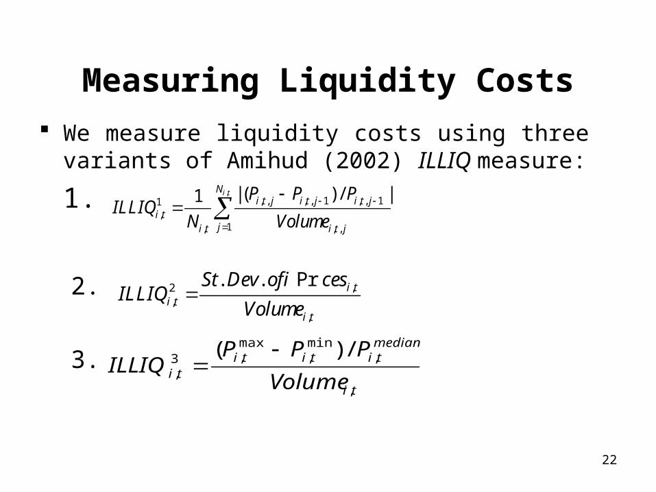
Measuring Liquidity Costs

We measure liquidity costs using three variants of Amihud (2002) ILLIQ measure:

1.

2.

3.

,2,

,

. . Pr i ti t

i t

St Dev of icesILLIQ

Volume

ti

mediantititi

ti Volume

PPPILLIQ

,

,min,

max,3

,

/)(

,, , , , 1 , , 11

,1, , ,

| ( ) / |1 i tNi t j i t j i t j

i tji t i t j

P P PILLIQ

N Volume

23

Empirical Methodology

We construct equal-weighted portfolios to be used as test assets (to remove the effect of noise embedded in individual securities)

These portfolios are created based on three criteria:- maturity- credit rating- illiquidity

We also construct an equal-weighted market-wide portfolio We then compute ILLIQ, and innovations in ILLIQ (because of persistence

in illiquidity) for each portfolio in each trading week (equal-weighting) We use the following specification for the innovations (similar to Acharya

and Pedersen (2005) & Pastor and Stambaugh (2003)):

We then estimate the liquidity betas (over entire sample period)

0 1 1 2 2=p p pt t t tILLIQ ILLIQ ILLIQ

24

ILLIQ1 ILLIQ2 ILLIQ3

Panel A : Time-series average, followed by cross-sectional average

ILLIQ1 1.00

ILLIQ2 0.50 1.00(<.0001)

ILLIQ3 0.52 0.99 1.00(<.0001) (<.0001)

Panel B : Cross-sectional average, followed by time-series average

ILLIQ1 1.00

ILLIQ2 0.47 1.00(<.0001)

ILLIQ3 0.50 0.98 1.00(<.0001) (<.0001)

Table IVCorrelation of Bond Illiquidity Measures

25

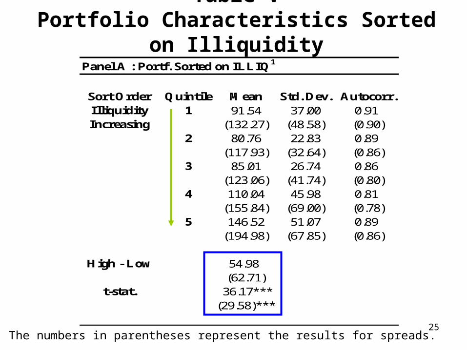
Panel A : Portf. Sorted on ILLIQ1

Sort Order Quintile Mean Std. Dev. Autocorr.Illiquidity 1 91.54 37.00 0.91Increasing (132.27) (48.58) (0.90)

2 80.76 22.83 0.89(117.93) (32.64) (0.86)

3 85.01 26.74 0.86(123.06) (41.74) (0.80)

4 110.04 45.98 0.81(155.84) (69.00) (0.78)

5 146.52 51.07 0.89(194.98) (67.85) (0.86)

High - Low 54.98(62.71)

t-stat. 36.17***(29.58)***

Table VPortfolio Characteristics Sorted on Illiquidity

The numbers in parentheses represent the results for spreads.

26

Panel C : Portf. Sorted on Maturity and ILLIQ1

Illiquidity Increasing1 2 3 4 5 Portf. 5 - 1 t-stat.

Maturity 1 76.72 67.70 74.55 94.09 143.14 66.41 24.99***Increasing (37.57) (29.31) (18.16) (31.22) (48.03) (38.42)

2 73.89 57.17 66.31 85.64 118.29 44.39 17.99***(45.85) (31.54) (46.12) (61.33) (49.64) (35.68)

3 103.40 98.27 88.27 106.21 140.41 37.01 8.44***(72.41) (87.59) (67.07) (84.51) (102.66) (63.40)

4 105.59 106.71 101.09 117.11 143.27 37.68 7.54***(40.56) (33.55) (40.78) (71.48) (99.49) (72.21)

5 105.34 108.05 126.78 148.48 157.49 52.16 25.57**(29.64) (29.20) (35.68) (48.50) (48.31) (29.48)

Panel D : Portf. Sorted on Credit Rating and ILLIQ1

Illiquidity IncreasingRating 1 2 3 4 5 Portf. 5 - 1 t-stat.AAA 51.42 48.52 49.87 54.53 71.80 20.39 7.33***

(33.80) (55.47) (46.87) (18.21) (22.66) (39.44)AA 60.40 51.02 52.00 61.60 77.65 17.43 7.88***

(26.53) (20.94) (19.11) (17.88) (21.44) (31.89)A 61.52 56.67 61.67 71.56 95.68 34.16 42.10***

(14.50) (12.59) (13.12) (15.09) (11.86) (11.73)BBB 91.67 86.13 101.28 121.97 144.82 53.15 24.24***

(40.03) (24.25) (33.44) (42.84) (36.66) (31.70)JUNK 235.40 234.31 246.76 295.15 351.29 115.89 9.78***

(78.79) (80.02) (120.33) (154.57) (197.29) (171.25)

Table VIPortfolio Characteristics Sorted on Maturity &

Illiquidity, and Credit Rating & Illiquidity Excess Returns (Standard Deviation)

27

Standardized Innovations in Market Illiquidity

Figure 1: Standardized Innovations of MarketIlliquidity

-6

-4

-2

0

2

4

6

8

2003

2003

2003

2003

2004

2004

2004

2005

2005

2005

2005

2006

2006

2006

Time (Jan. 1, 2003 - Dec. 31, 2006)

Inn

ova

tio

ns

in M

arke

tIl

liq

uid

ity ILLIQ1

ILLIQ2

ILLIQ3

28

Section A: ILLIQ1 Section B: ILLIQ2

β βL1 βL2 βL3 E(cp) β βL1 βL2 βL3 E(cp)

Panel A: Portfolios sorted on illiquidity1 0.61 0.02 -1.87 0.03 0.39 0.28 0.03 -2.53 -0.01 0.192 0.27 0.37 -0.96 0.19 4.75 0.36 0.15 -3.96 -0.03 0.793 0.28 1.06 0.82 0.29 17.55 0.73 0.50 -5.68 -0.09 2.554 0.39 2.19 -0.05 0.57 44.76 0.47 1.80 -4.35 -0.24 9.755 0.69 13.90 -2.39 0.01 192.53 0.43 14.90 -3.25 -3.53 99.44

Panel B: Portfolios sorted on maturity and illiquidity1.1 0.27 0.01 -0.51 0.01 0.20 0.41 0.02 1.72 -0.01 0.141.5 0.95 5.49 2.51 1.11 109.64 0.85 7.57 -1.02 -2.66 57.602.1 0.64 -0.01 -1.68 0.06 0.58 0.87 0.03 -7.35 0.00 0.222.5 0.88 12.56 -0.35 1.06 140.49 0.27 8.50 -1.53 -1.91 71.923.1 1.11 0.09 1.50 0.21 1.00 1.09 0.05 -12.16 -0.01 0.233.5 1.48 11.65 0.23 3.40 165.80 1.34 9.45 -17.60 -1.38 69.094.1 0.28 0.01 -2.34 0.00 0.40 0.23 0.03 -3.04 0.00 0.154.5 -0.31 9.96 1.25 -0.61 167.24 0.75 8.99 -3.92 0.32 67.715.1 0.48 0.10 -2.25 0.17 0.78 0.97 0.12 -0.30 -0.01 0.395.5 0.65 26.25 -5.62 -2.09 337.02 0.52 34.05 0.47 -6.62 214.30

Panel C: Portfolios sorted on credit rating and illiquidityAAA,1 0.02 0.07 0.49 -0.06 0.80 -0.06 0.06 0.42 -0.01 0.26AAA,5 -0.04 25.17 2.08 5.44 201.15 -0.17 15.13 2.48 4.99 135.73AA,1 0.22 0.36 1.08 5.19 0.50 0.20 0.03 2.30 -0.01 0.19AA,5 -0.25 3.51 1.98 -3.48 163.45 -0.36 19.66 4.42 -7.02 95.11A,1 0.10 -0.03 -0.43 2.58 0.58 0.16 0.03 6.31 -0.01 0.21A,5 0.10 14.06 1.81 -2.05 190.11 -0.10 13.34 0.66 -3.18 97.47

BBB,1 0.06 0.39 2.11 -1.30 0.31 -0.24 0.03 1.42 0.00 0.11BBB,5 0.24 12.68 6.91 0.86 188.38 -0.04 21.46 3.16 -7.07 95.38JUNK,1 -0.36 -0.32 3.48 0.79 0.64 -0.91 0.06 -8.14 0.00 0.27JUNK,5 -0.74 13.29 26.20 2.25 172.00 -0.77 5.12 -7.86 3.57 54.73

Table VIIBetas on Test Portfolios (for Excess Returns)

29

Section C: ILLIQ3

β βL1 βL2 βL3 E(cp)

Panel A: Portfolios sorted on illiquidity1 0.13 0.08 -0.83 -0.01 0.632 0.15 0.40 -2.26 -0.03 2.523 0.15 1.28 -4.29 -0.08 7.814 0.22 4.34 -5.55 -0.21 28.225 0.16 29.67 -2.96 -2.73 248.61

Panel B: Portfolios sorted on maturity and illiquidity1.1 0.26 0.04 0.69 -0.01 0.431.5 0.34 13.89 -0.14 -1.68 142.422.1 0.07 0.08 -3.07 0.01 0.772.5 0.26 16.60 -3.38 -1.25 179.883.1 0.07 0.14 -4.92 -0.02 0.823.5 0.04 19.29 -17.46 -1.13 174.224.1 -0.07 0.10 0.28 0.00 0.524.5 0.34 18.32 -5.53 0.26 170.335.1 0.42 0.34 -1.26 -0.01 1.215.5 0.35 67.61 1.23 -5.12 528.21

Panel C: Portfolios sorted on credit rating and illiquidityAAA,1 -0.02 0.12 0.37 -0.01 0.88AAA,5 -0.06 19.83 2.06 2.76 307.48AA,1 0.07 0.08 2.09 -0.01 0.65AA,5 -0.13 34.81 3.85 -6.37 223.73A,1 0.05 0.07 5.30 -0.01 0.70A,5 -0.03 26.29 0.45 -2.62 240.64

BBB,1 -0.09 0.07 0.99 0.00 0.36BBB,5 -0.01 39.37 2.96 -4.33 238.79

JUNK,1 -0.33 0.16 -2.89 0.00 0.99JUNK,5 -0.30 15.64 -7.63 3.84 154.81

Table VIIBetas on Test Portfolios (Excess Returns)

30

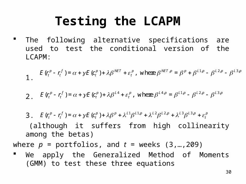
Testing the LCAPM The following alternative specifications are used to test the

conditional version of the LCAPM:

1.

2.

3.

(although it suffers from high collinearity among the betas)

where p = portfolios, and t = weeks (3,…,209) We apply the Generalized Method of Moments (GMM) to test

these three equations

, 1, 2, 3,( ) = ( ) , where =p f p NET p NET p p L p L p L pt t t tE r r E c

4 4, 1, 2, 3,( ) = ( ) , where =p f p L p L p L p L p L pt t t tE r r E c

1 1, 2 2, 3 3,( ) = ( )p f p p L L p L L p L L p pt t t tE r r E c

31

Table VIIIGMM Estimation of LCAPM (Excess Returns)

Section A : ILLIQ1

Intercept E(cp) β βL1 βL2 βL3 βL4 βNET Adj. R2

Panel A : Portfolios sorted on illiquidity1 84.61 -0.03 3.95 0.279

(57.00)*** (0.58) (6.37)***2 86.05 -0.04 4.1 0.279

(59.31)*** (0.68) (6.31)***3 48.74 -0.41 57.93 9.32 -2.45 60.89 0.345

(15.99)*** (5.49)*** (9.31)*** (8.75)*** (3.25)*** (9.76)***

Panel B: Portfolios sorted on maturity and illiquidity1 90.56 0.14 1.37 0.127

(97.21)*** (4.00)*** (4.03)***2 90.99 0.14 1.30 0.125

(97.53)*** (4.19)*** (3.76)***3 86.36 0.23 4.47 -0.16 -3.69 4.41 0.139

(68.77)*** (3.82)*** (2.18)** (0.21) (8.17)*** (3.04)***

Panel C: Portfolios sorted on credit rating and illiquidity1 60.79 0.70 -9.83 0.379

(29.99)*** (20.04)*** (24.86)***2 60.53 0.14 1.30 0.369

(29.29)*** (19.87)*** (24.34)***3 59.42 0.11 -45.79 -1.58 11.31 1.21 0.482

(27.68)*** (3.50)*** (12.68)*** (4.43)*** (23.09)*** (2.74)***

32

Table VIIIGMM Estimation of LCAPM (Excess Returns)

Section B : ILLIQ2

Intercept E(cp) β βL1 βL2 βL3 βL4 βNET Adj. R2

Panel A : Portfolios sorted on illiquidity1 70.12 -0.66 5.59 0.176

(22.35)*** (5.17)*** (8.01)***2 71.93 -0.68 5.76 0.176

(24.04)*** (5.22)*** (7.97)***3 61.65 -0.63 -47.59 10.33 -13.3 13.43 0.180

(14.98)*** (3.95)*** (3.65)*** (3.00)*** (6.15)*** (1.01)

Panel B: Portfolios sorted on maturity and illiquidity1 96.33 0.01 1.05 0.024

(60.34)*** (0.30) (3.69)***2 97.36 0.03 0.94 0.023

(63.74)*** (0.65) (3.37)***3 94.47 -0.33 10.34 4.81 -0.27 5.96 0.050

(53.81)*** (4.45)*** (4.85)*** (8.48)*** (0.97) (4.97)***

Panel C: Portfolios sorted on credit rating and illiquidity1 110.02 -0.19 2.17 0.013

(45.50)*** (4.76)*** (9.90)***2 108.11 -0.31 3.37 0.032

(46.31)*** (5.74)*** (12.67)***3 89.93 -0.06 -101.11 1.38 -11.11 -2.05 0.484

(66.61)*** (1.92)** (36.62)*** (4.55)*** (20.22)*** (3.54)***

33

Table VIIIGMM Estimation of LCAPM (Excess Returns)

Section C : ILLIQ3

Intercept E(cp) β βL1 βL2 βL3 βL4 βNET Adj. R2

Panel A : Portfolios sorted on illiquidity1 101.84 -0.11 2.37 0.115

(30.73)*** (1.31) (2.84)***2 102.14 -0.11 2.34 0.114

(29.81)*** (1.27) (2.80)***3 32 -0.3 313.83 -13.88 -6.97 -188.29 0.230

(2.38)** (3.52)*** (2.97)*** (3.19)*** (6.40)*** (4.25)***

Panel B: Portfolios sorted on maturity and illiquidity1 104.53 -0.04 1.20 0.045

(72.25)*** (2.58)*** (9.40)***2 104.74 -0.03 1.18 0.044

(71.80)*** (2.38)** (9.20)***3 86.00 -0.14 37.08 2.86 -0.77 10.97 0.089

(52.91)*** (3.96)*** (9.70)*** (8.73)*** (2.44)*** (5.47)***

Panel C: Portfolios sorted on credit rating and illiquidity1 113.83 0.12 -1.25 0.008

(42.89)*** (4.58)*** (5.30)***2 113.2 0.10 -0.97 0.006

(42.82)*** (4.18)*** (4.42)***3 83.43 -0.1 -242.34 2.58 -11.53 5.7 0.496

(63.05)*** (4.40)*** (26.32)*** (8.59)*** (19.25)*** (4.81)***

34

Robustness Tests

• Exclude the callable bonds and rerun the tests (callable bonds constitute almost half of the sample).

• Rearrange the rating groups to have a more representative number of transactions in each bucket (e.g. 1st bucket: ‘AAA, AA+, AA, AA-, A+’, 2nd bucket: ‘A, A-’, etc.).

• Construct portfolios/market returns and illiquidity using a value-weighted approach (based on bond amount outstanding).

• Because of the different phases of TRACE, we separate the sample into the partial-information sample (prior to Feb. 7th, 2005) and the full sample (between Feb. 2005, and end of December, 2006) and re-run our tests.

• TRACE suffers from the fact that it truncates the volume of the transaction (above 5MM for IG, and 1MM for HY). We therefore exclude these transactions and rerun the tests.

35

Robustness Tests…• Construct a weekly return-based measure (for every issue) based

on Downing et al. (2005):

• Normalize the ILLIQ measure similar to Acharya and Pedersen (2005):

where stands for the ratio of capitalizations between end of week t-1, and end of week 1.– The normalization makes the ILLIQ fairly stationary.

• Use various restrictions (minimum number of observations) in constructing the ILLIQ measure.

( ) /i last first firstt t t tr p p p

1min[0.25 0.30* * ]i i Mt t tc ILLIQ P

1M

tP

36

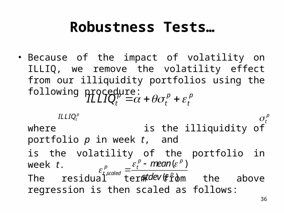
Robustness Tests…

• Because of the impact of volatility on ILLIQ, we remove the volatility effect from our illiquidity portfolios using the following procedure:

where is the illiquidity of portfolio p in week t, and

is the volatility of the portfolio in week t.

The residual term from the above regression is then scaled as follows:

p p pt t tILLIQ

,

( )

( )

p pp t

t scaled p

mean

stdev

ptILLIQ p

t

37

Other Tests

• Following the papers by Chordia, Sarkar, and Subrahmanyam (2005) and Goyenko (2005) where they document a spillover of illiquidity, we include in our GMM regression three liquidity betas of each portfolio with respect to the Treasury market, three liquidity betas with respect to the equity markets, as well as the PIN [Easley, Kiefer, O’Hara, and Paperman (1996)] from equity data and Roll’s (1984) negative serial covariance of price changes measure (for bonds). The resulting specification is as follows:

, 4,_ _

4,_

, 1, 2, 3,_

4, 1, 2, 3,_

4,_

( ) = ( )

,

where =

=

=

p f p NET p L pt t t CORP MARKET TREAS MARKET

L p p p pEQUITY MARKET t t t

NET p p L p L p L pCORP MARKET

L p L p L p L pTREAS MARKET

L p LEQUITY MARKET

E r r E c

PIN ROLL

1, 2, 3,p L p L p

38

Other Tests…

• The Treasury market illiquidity & return is computed as follows:– Using a Treasury market index from Bloomberg that includes domestically i

ssued fixed rate government bonds (bullets, callable, and puttable issues are also included) of minimum size of $2 billion, we construct a weekly Treasury market return.

– Combining the weekly Treasury market return with weekly Treasury volume data provided by the New York Fed’s website (primary dealer transactions on U.S. government securities with inter-dealer brokers & others), we construct a proxy for the weekly Treasury market illiquidity (ILLIQ).

• The equity market illiquidity & return is computed as follows:– Using CRSP database we compute the weekly equity market return.

– Using TAQ and CRSP we compute the effective half-spread (distance between the quote midpoint prior to a trade and the trade price) for each stock, and then take a cross-sectional average to get a weekly equity market liquidity. We also compute the Amihud measure.

39

Conclusions

• Univariate analysis shows that, after controlling for maturity & credit rating, portfolio returns/spreads increase with illiquidity.

• On average, more illiquid portfolios tend to have higher values for the three illiquidity betas.

• Cross-sectional regressions provide evidence that liquidity risk arising from the corporate bond market is priced in the U.S. corporate bonds.

• Results, on average, seem to be robust for all illiquidity measures used.

40

Thank You