1 lecture 6 first order circuits (i). linear time-invariant first-order circuit, zero input...
Post on 20-Dec-2015
232 views
TRANSCRIPT

1
Lecture 6Lecture 6
First order Circuits (i).
Linear time-invariant first-order circuit, zero input response.
The RC circuits.
•Charging capacitor
•Discharging capacitor
The RL circuits.
The zero-input response as a function of the initial state.
Mechanical examples.
Zero-state response (Constant current input, Sinusoidal input).
Complete response: transient and steady-state.
2
Why first order?
In this lecture we shall analyze circuits with more than one kind of element; as a consequence, we shall have to use differentiation and/or integration.
We shall restrict ourselves here to circuits that can be described by first-order differential equations; hence we give them the name first-order circuitsfirst-order circuits
3
Linear Time –invariant First order Circuit. Linear Time –invariant First order Circuit. Zero-input ResponseZero-input Response
TheThe RCRC Circuits Circuits
k2
RC
kk11
v=Vv=V00
E=VE=V0 0
i(t)i(t)+
_
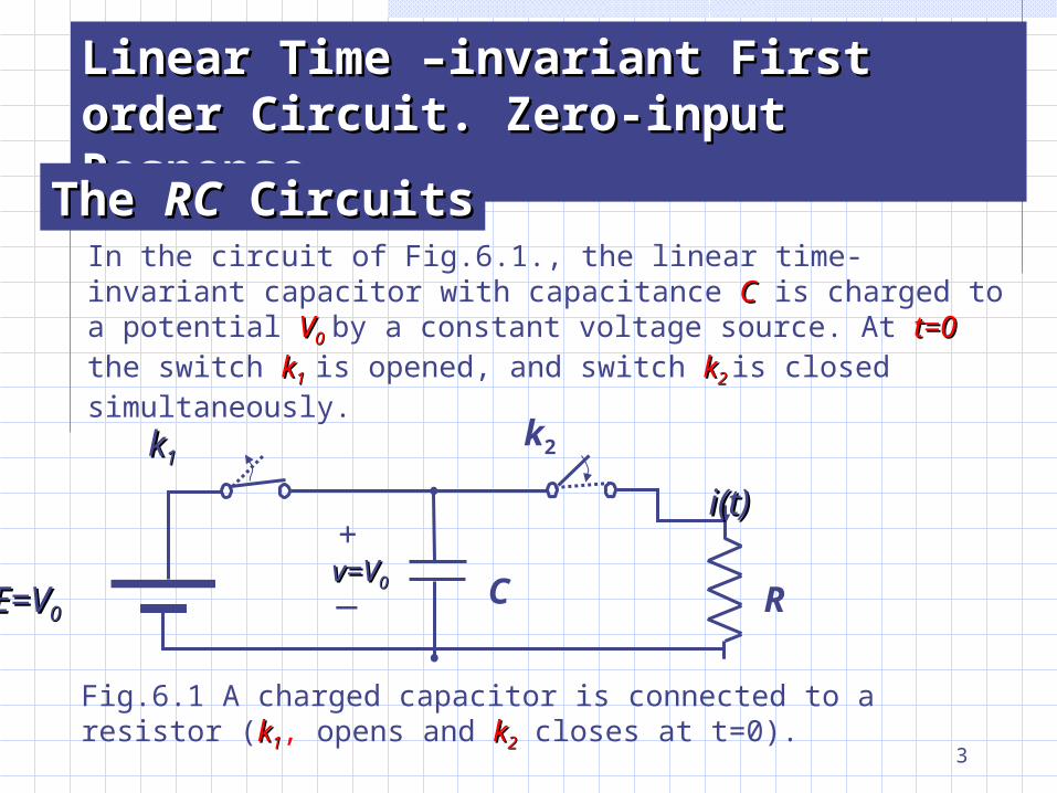
Fig.6.1 A charged capacitor is connected to a resistor (kk11, opens and kk22 closes at t=0).
In the circuit of Fig.6.1., the linear time-invariant capacitor with capacitance CC is charged to a potential VV00 by a constant voltage source. At t=0t=0 the switch kk11 is opened, and switch kk2 2 is closed simultaneously.
4
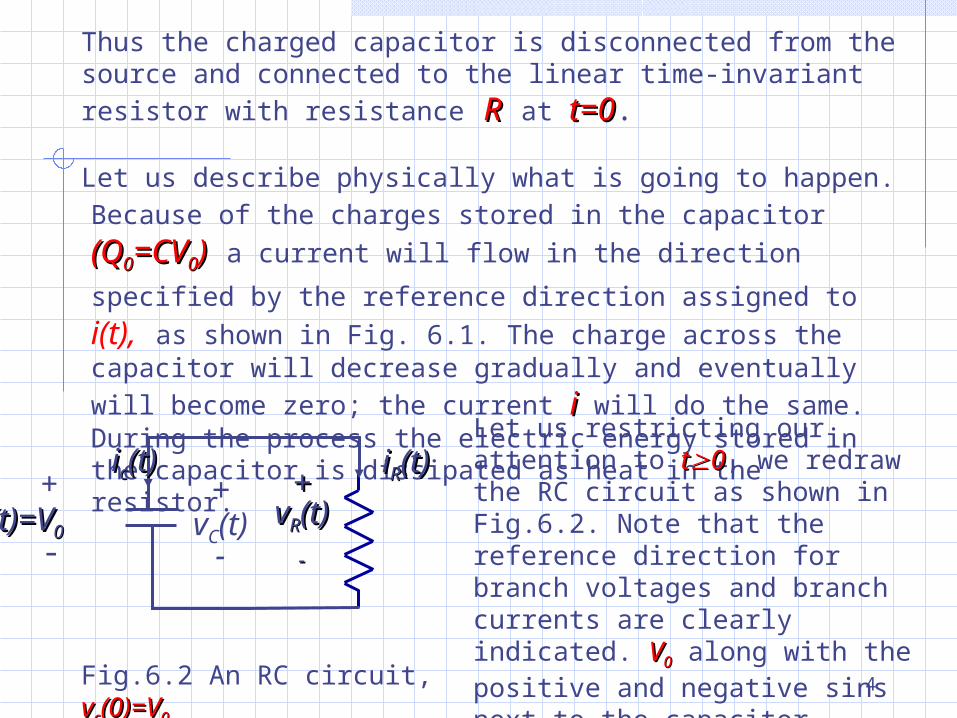
Thus the charged capacitor is disconnected from the source and connected to the linear time-invariant resistor with resistance RR at t=0t=0.
Let us describe physically what is going to happen. Because of the charges stored in the capacitor (Q(Q00=CV=CV00)) a current will flow in the direction specified by the reference direction assigned to i(t), as shown in Fig. 6.1. The charge across the capacitor will decrease gradually and eventually will become zero; the current ii will do the same. During the process the electric energy stored in the capacitor is dissipated as heat in the resistor.
Fig.6.2 An RC circuit, vvcc(0)=V(0)=V00
iiRR(t)(t)++
vvRR(t)(t)
--
+vC(t)
-
+vvcc(t)=V(t)=V00
-
iicc(t)(t)Let us restricting our attention to tt00, we redraw the RC circuit as shown in Fig.6.2. Note that the reference direction for branch voltages and branch currents are clearly indicated. VV00 along with the positive and negative sins next to the capacitor, specifies the magnetite and polarity of the initial voltage.

5
Kirchoff`’s laws and topology dictate the following equations:
0 )()( ttvtv RC (6.1)KVL:
KCL: 0 0)()( ttiti RC(6.2)
The two branch equations for the two circuit elements are
Resistor: RR Ritv )( (6.3)
Capacitor: 0 and Vvdt
dvCi C
CC (6.4a)
or, equivalently
tdtiC
Vvt
CC )(1
0
0(6.4b)
In Eq.(6.4a) we want to emphasize that the initial condition
6
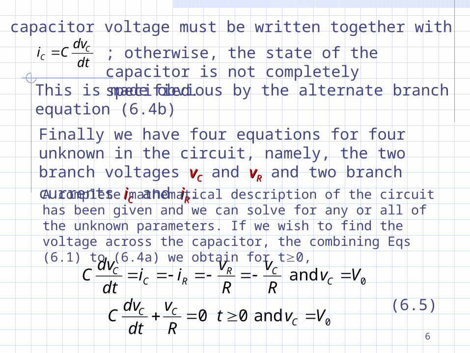
Of the capacitor voltage must be written together with
dt
dvCi C
C ; otherwise, the state of the capacitor is not completely specified.
This is made obvious by the alternate branch equation (6.4b)
Finally we have four equations for four unknown in the circuit, namely, the two branch voltages vvCC and vvRR and two branch currents iiCC and iiRR. A complete mathematical description of the circuit has been given and we can solve for any or all of the unknown parameters. If we wish to find the voltage across the capacitor, the combining Eqs (6.1) to (6.4a) we obtain for t0,
0 and VvR
v
R
vii
dt
dvC C
CRRC
C
0 and 0 0 VvtR
v
dt
dvC C
CC (6.5)

7
This is a first-order linear homogeneous differential equation with constant coefficients. Its solution is of the exponential form
This easily verified by direct substitution of Eqs. (6.6) and (6.7) in the differential equation (6.5). In (6.6) K is a constant to be determined from the initial conditions. Setting t=0t=0 in Eq.(6.6), we obtain vvCC(0)=K=V(0)=K=V00. Therefore, the solution to the problem is given by
tsC Ketv 0)( (6.6)
where
RCs
10
0 )(1
0
teVtvt
RCC
(6.7)
(6.8)

8
In Eq.(6.8), vvCC(t)(t) is specified for tt00 since for negative t the voltage across the capacitor is a constant, according to our original physical specification.
RCTeVtv TtC )( /
0
00 TT 2T2T 3T3T 4T4T tt
vvCC
VV00
0.377V0.377V00
Fig.6.3 The discharge of the Capacitor of Fig. 6.2 is given by an experimental curve
The voltage vvCC(t)(t) is plotted in Fig. 6.3 as a function of time. Of course, we can immediately the other three branch variables once vvCC(t)(t) is known. From Eq.(6.4a) we have
0 )(1
0
t eR
V
dt
dvCti
tRCC
C (6.9)From Eq.(6.2) we have
0 )()(1
0
t eR
Vtiti
tRC
CR(6.10)
From Eq. (6.3) we have
0 )()(1
0
t eVtvtvt
RCRC
(6.11)

9
0
tt
R
V0
iiCC
R
V0iiRR
vvRR0V
tt
tt
Fig.6.4. Network variables iiCC ,i ,iRR and vvR R
against time for t0.
Exercise Show that the red line in Fig. 6.3, which is tangent to the curve vc(t)=0+, intersects the time axis at the abscissa T
10
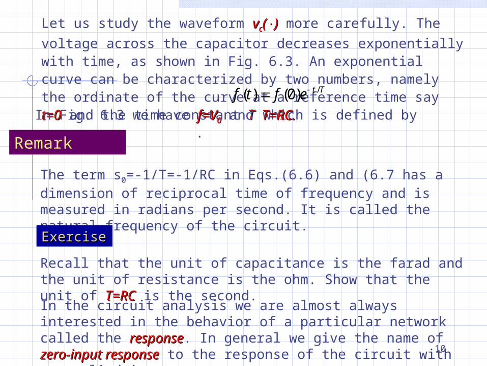
Let us study the waveform vvcc(()) more carefully. The voltage
across the capacitor decreases exponentially with time, as shown in Fig. 6.3. An exponential curve can be characterized by two numbers, namely the ordinate of the curve at a reference time say t=0t=0 and the time constant TT which is defined by .
Tteftf /)0()( In Fig. 6.3 we have f=Vf=V00 and T=RC.T=RC.
Remark
The term s0=-1/T=-1/RC in Eqs.(6.6) and (6.7 has a dimension of reciprocal time of frequency and is measured in radians per second. It is called the natural frequency of the circuit.
ExerciseExercise
Recall that the unit of capacitance is the farad and the unit of resistance is the ohm. Show that the unit of T=RCT=RC is the second.In the circuit analysis we are almost always interested in the behavior of a particular network called the responseresponse. In general we give the name of zero-input responsezero-input response to the response of the circuit with no applied input
11
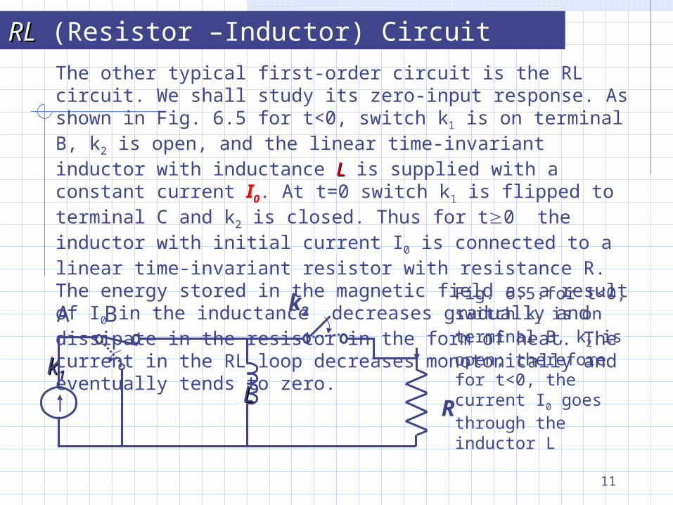
The RLRL (Resistor –Inductor) Circuit
k2
R
kk11
II0 0
LL
A B
The other typical first-order circuit is the RL circuit. We shall study its zero-input response. As shown in Fig. 6.5 for t<0, switch k1 is on terminal B, k2 is open, and the linear time-invariant inductor with inductance LL is supplied with a constant current I0. At t=0 switch k1 is flipped to terminal C and k2 is closed. Thus for t0 the inductor with initial current I0 is connected to a linear time-invariant resistor with resistance R. The energy stored in the magnetic field as a result of I0 in the inductance decreases gradually and dissipate in the resistor in the form of heat. The current in the RL loop decreases monotonically and eventually tends to zero.
Fig. 6.5.for t<0, switch k1 is on terminal B, k2 is open; therefore for t<0, the current I0 goes through the inductor L
12
iiRR
++vvRR
--
+vL(t)
-iiLL(0)=I(0)=I00
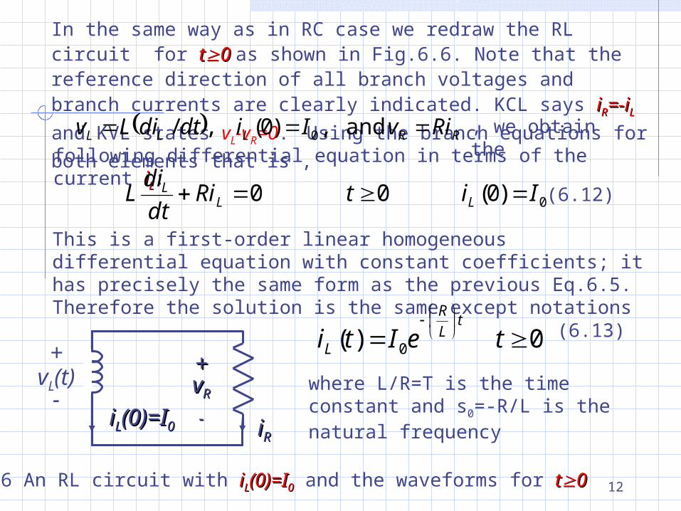
In the same way as in RC case we redraw the RL circuit for tt0 0 as shown in Fig.6.6. Note that the reference direction of all branch voltages and branch currents are clearly indicated. KCL says iiRR=-i=-iLL and KVL states vL-vR=0. Using the branch
equations for both elements that is , RRLLL RivIidtdiLv and ,)0( ,/ 0 , we obtain the
following differential equation in terms of the current iiLL:
0)0( 0 0 IitRidt
diL LL
L (6.12)
Fig.6.6 An RL circuit with iiLL(0)=I(0)=I00 and the waveforms for tt00
This is a first-order linear homogeneous differential equation with constant coefficients; it has precisely the same form as the previous Eq.6.5. Therefore the solution is the same except notations
0 )( 0
teItit
L
R
L(6.13)
where L/R=T is the time constant and s0=-R/L is the natural frequency
13
The zero-input response as a function of the initial stateThe zero-input response as a function of the initial state
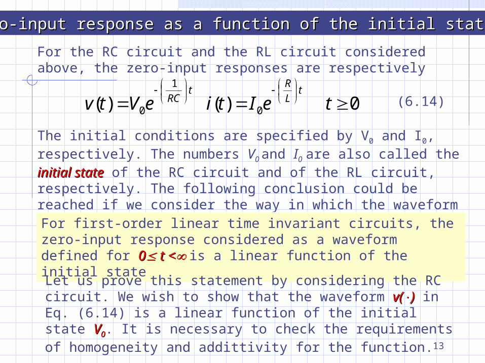
For the RC circuit and the RL circuit considered above, the zero-input responses are respectively
0 )( )( 0
1
0
teItieVtvt
L
Rt
RC (6.14)
The initial conditions are specified by V0 and I0, respectively. The numbers V0 and I0 are also called the initial stateinitial state of the RC circuit and of the RL circuit, respectively. The following conclusion could be reached if we consider the way in which the waveform of the zero-input response depends on the initial state.For first-order linear time invariant circuits, the zero-input response considered as a waveform defined for 00 t < t < is a linear function of the initial state
Let us prove this statement by considering the RC circuit. We wish to show that the waveform v(v()) in Eq. (6.14) is a linear function of the initial state VV00. It is necessary to check the requirements of homogeneity and addittivity for the function.
14
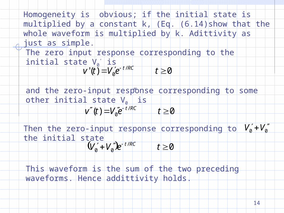
Homogeneity is obvious; if the initial state is multiplied by a constant k, (Eq. (6.14)show that the whole waveform is multiplied by k. Adittivity as just as simple.
The zero input response corresponding to the initial state V0’
is 0 )(' /
0 teVtv RCt
and the zero-input response corresponding to some other initial state V0” is
0 )( /0 teVtv RCt
Then the zero-input response corresponding to the initial state
00 VV
0 /00 teVV RCt
This waveform is the sum of the two preceding waveforms. Hence addittivity holds.

15
Remark
This property does not hold in the case of nonlinear circuits. Consider the RC circuit shown in Fig. 6.7a. The capacitor is linear and time invariant and has a capacitance of 1 farad, and the resistor is nonlinear with characteristic
3RR vi
The two elements have the same voltage v, and expressing the branch currents in terms of v, we obtain from KCL
03 )0( 0 Vvv
dt
dvi
dt
dvC R
iiRR++vvRR
--
+v-
C=1 FC=1 F
Hencedt
v
dv
3
If we integrate between 0 an t, the voltage takes the initial value V0 and the final value v(t); hence
Fig.6.7a Nonlinear RC circuit and two of its zero-input resistance. The capacitor is linear and the resistor 3
RR vi

16
tVtv
2
02 2
1
)(2
1
or0
21)(
20
0
ttV
Vtv
This is the zero-input response of this nonlinear RCRC circuit starting from the initial state VV00 at time 0. The waveforms corresponding to VV00=0.5=0.5 and VV00=2=2 are plotted in Fig 6.7b.
VV00=2=2
VV00=0.5=0.5
03 vdt
dv
0.5
2.0
1.0
1.5
21
)(2
0
0
tV
Vtv
tt
vv
Fig. 6.7b
It is obvious that the top curve (VV00=2=2) cannot be obtained from the lower one (for VV00=0.5=0.5) by multiplying its ordinates by 4.
(6.15)

17
Mechanical example
Let us consider a familiar mechanical system that has a behavior similar to that of the linear time invariant RCRC and RLRL circuits above.
MMv(t) v(0)=Vv(t) v(0)=V00
Bv (friction forces)Bv (friction forces)
Fig. 6.8 A mechanical system which is described by a first order differential equation
Figure 6.8 shows a block of mass MM moving at an initial velocity VV00 at t=0t=0.
As time proceeds, the block will slow down gradually because friction tends to oppose the motion. Friction is represented by friction forces that are all ways in the direction opposite to the velocity v, as shown in the figure. Let us assume that these forces are proportional to the magnitude of the velocity; thus, f=Bvf=Bv, where the constant BB is called the damping coefficient. From Newton’s second law of motion we have, for tt0,0,
18
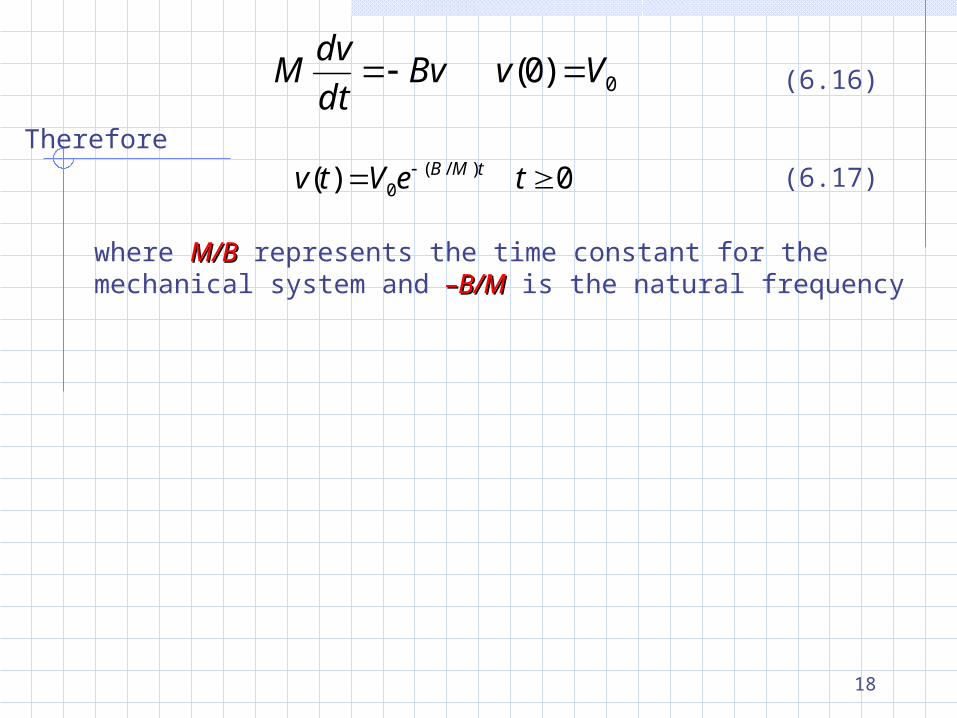
0)0( VvBvdt
dvM (6.16)
Therefore
0 )( )/(0 teVtv tMB (6.17)
where M/BM/B represents the time constant for the mechanical system and –B/M–B/M is the natural frequency

19
Zero-state ResponseZero-state Response
Constant Current Input
Rkkiiss(t)=I(t)=I CC
Fig.6.9 RC circuit with current source input. At t=0, switch k is opned
In the circuit of Fig. 6.9 a current source iiss is switched to a parallel linear time invariant RC circuit. For simplicity we consider first the case when the current iiss is constant and equal to II. Prior to the opening of the switch the current source produces a circulating current in the short circuit. At t =0, the switch is opened and thus the current source is connected the RC circuit. From KVL we see that the voltage across all three elements is the same. Let us design this voltage by vv and assume that vv is the response of interest. Writing the KCL equation in terms of v, we obtain the following network equation:
20
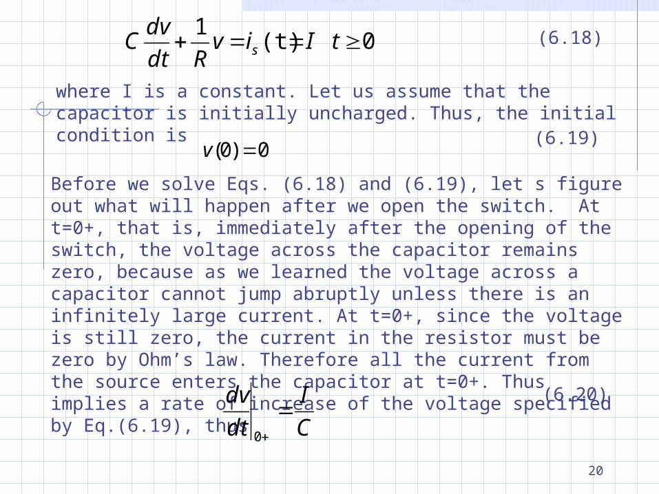
0 (t)1
tIivRdt
dvC s
(6.18)
where I is a constant. Let us assume that the capacitor is initially uncharged. Thus, the initial condition is
0)0( v(6.19)
Before we solve Eqs. (6.18) and (6.19), let s figure out what will happen after we open the switch. At t=0+, that is, immediately after the opening of the switch, the voltage across the capacitor remains zero, because as we learned the voltage across a capacitor cannot jump abruptly unless there is an infinitely large current. At t=0+, since the voltage is still zero, the current in the resistor must be zero by Ohm’s law. Therefore all the current from the source enters the capacitor at t=0+. Thus implies a rate of increase of the voltage specified by Eq.(6.19), thus
C
I
dt
dv
0
(6.20)

21
As time proceeds, vv increases, and v/Rv/R, the current through the resistor, increases also. Long after the switch is opened the capacitor is completely charged, and the voltage is practically constant. Then and thereafter, dv/dtdv/dt00. All the current from the source goes through the resistor, and the capacitor behaves as an open circuit, that is
RIv (6.21)This fact is clear form Eq.(6.18), and it is also shown in Fig.6.10. The circuit is said to have reached a steady state. It only remains to show how the whole change of voltage takes place. For that we rely on the following analytical treatment.
v
RI
t
C
I:Slope
The solution of a linear no homogeneous differential equation can be written in the following form:
ph vvv (6.22)
Fig. 6.10. Initial and final behavior of the voltage across the capacitor.

22
The general solution of the homogeneous equation is of the form
RCseKv ts
h
1 01
0 (6.23)
where K1 is any constant. The most convenient particular solution for a constant current input is a constant
RIvp (6.24)
since the constant RI satisfies the differential equation (6.18). Substituting (6.23) and (6.24) in (6.22), we obtain the general solution of (6.18)
011 RI teKv(t) /RC)t( (6.25)
where K1 is to be evaluated from the initial condition specified by Eq.(6.19). Setting t=0 in (6.25), we have
where vvhh is a solution of the homogeneous differential equation and vvpp is any particular solution of the nonhomogenous differential equation. vvpp depends on the input.
23
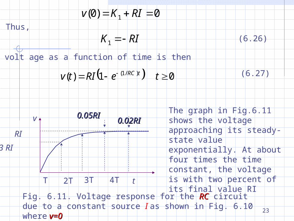
Thus,
RIK 1(6.26)
The volt age as a function of time is then
0 1)( )/1( teRItv tRC (6.27)
v
RI
t
Fig. 6.11. Voltage response for the RCRC circuit due to a constant source I as shown in Fig. 6.10 where v=0v=0
0)0( 1 RIKv
0.02RI0.02RI
4T3T
0.05RI0.05RI
2TT
0.63 RI
The graph in Fig.6.11 shows the voltage approaching its steady-state value exponentially. At about four times the time constant, the voltage is with two percent of its final value RI
24
Exercise 1
Sketch with appropriate scales the zero state response of the of Fig.6.10 with
a. I=200 mA, R=1 k, and C=1F
b. I=2 mA, R=50 , and C=5 nF
Exercise 2
a. Calculate and sketch the waveforms ps() (the power delivered by the source), pR() (the power dissipated by the resistor) and EC(), (the energy stored in the capacitor)
b. Calculate the efficiency of the process, i.e the ratio of the energy eventually stored in the capacitor to the energy delivered by the source [ ]
dttps )(0
25
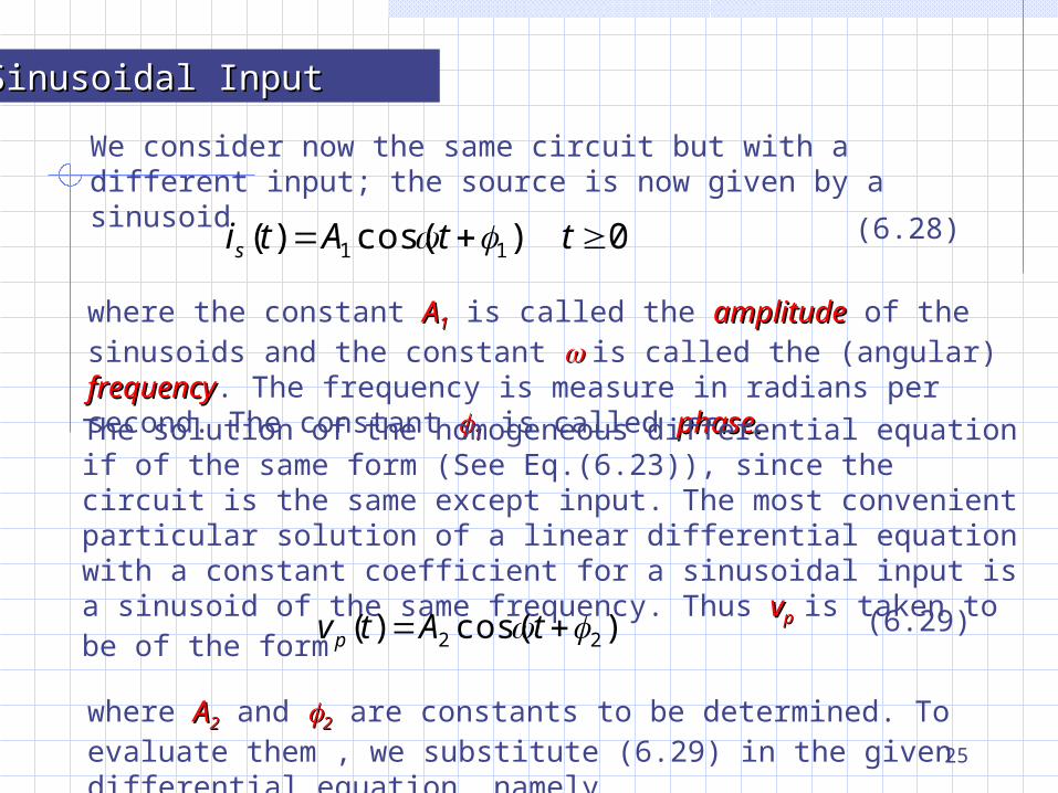
Sinusoidal InputSinusoidal Input
We consider now the same circuit but with a different input; the source is now given by a sinusoid
0 )cos()( 11 ttAtis (6.28)
where the constant AA11 is called the amplitudeamplitude of the sinusoids and the constant is called the (angular) frequencyfrequency. The frequency is measure in radians per second. The constant 11 is called phase.phase.The solution of the homogeneous differential equation if of the same form (See Eq.(6.23)), since the circuit is the same except input. The most convenient particular solution of a linear differential equation with a constant coefficient for a sinusoidal input is a sinusoid of the same frequency. Thus vvpp is taken to be of the form )cos()( 22 tAtvp
(6.29)
where AA22 and 22 are constants to be determined. To evaluate them , we substitute (6.29) in the given differential equation, namely
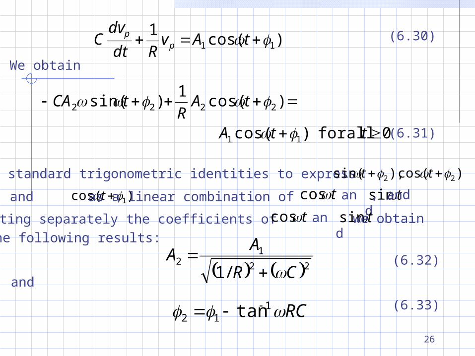
26
)cos(1
11 tAvRdt
dvC p
p (6.30)
We obtain
0 forall )cos(
)cos(1
)sin(
11
2222
ttA
tAR
tCA
(6.31)
Using standard trigonometric identities to express )cos(),sin( 22 tt
and )cos( 1 t as a linear combination of tcos and
tsin, and
equating separately the coefficients of tcos and
tsinwe obtain
the following results:
22
12
/1 CR
AA
(6.32)
and
RC 112 tan (6.33)

27
Here tantan-1-1RCRC denotes the angle between 0 and 90o whose tangent is equal to RCRC . This particular solution and the input current are plotted in Fig. 6.12.
AA11
1
2
iiss
tt
tt
tt11
AA22
111 tan
1
RCt
Fig.6.12 Input current and a particular solution for the output voltage of the RC circuit in Fig.6.9.
vvpp

28
Exercise
Derive Eqs. (6.32) and (6.33) in detail.
The general solution of (6.31) is therefore of the form
0 )cos()( 22/1
1 ttAeKtv tRC (6.34)
Setting t=0t=0, we have
cos)0( 221 AKv (6.35)
that is cos 221 AK (6.36)
Therefore the response is given by
0 )cos(cos)( 22/1
22 ttAeAtv tRC (6.37)
where AA22 and 22 are defined in Eqs.(6.32) and (6.33). The graph of vv, that is the zero-state response to the input AA11 cos( cos(t+t+11),), is plotted in Fig.6.13.

29
vv
ttvvhh
vvpp
v(t)v(t)
Fig.6.13. Voltage response of the circuit in Fig. 6.13 with v(0)=0v(0)=0 and iiss(t)=A(t)=A11cos(cos(t+t+11))
In the two cases treated in this lecture we considered the voltage vv as the response and the current source iiss as the input. The initial condition in the circuit is zero; that is, the voltage across the capacitor is zero before the application of the input. In general we say that a circuit is in the zero state is all the initial conditions in the circuit are zero. The response of a circuit which starts from the zero state, is due exclusively to the input. By definition, the zero-state response is the response of a circuit to an input applied at some arbitrary time, say, tt00, subject to the condition that the circuit be in the zero state just prior to the application of the input (that is, at time tt00--).
In calculating zero-state responses, our primary interest is the behavior of the response for tttt00. It means that the input and the zero-state response are taken to be identically zero at t<tt<t00.

30
Complete Response: Transient and Steady stateComplete Response: Transient and Steady state
Complete response.
The response of the circuit to both an input and the initial conditions is called the complete response of the circuit. Thus the zero-input response and the zero-state response are special cases of the complete response.
Let us demonstrate that for the simple linear RC circuit for the simple linear RC circuit considered, the complete response is the sum of the zero-considered, the complete response is the sum of the zero-input response and the zero-state response.input response and the zero-state response.
R
kk
iiss(t)(t)
CC
BB
AA VV00
+
-vv+
-
Fig.6.14 RC RC circuit with v(0)=Vv(0)=V00 is excited by a current source
iiss(t).(t). The switch kk is flipped from AA to BB at t=0t=0.
Consider the circuit in Fig. 6.14 where the capacitor is initially charged; that isv(0)=Vv(0)=V0000, and a current input is switched into the circuit at t=0.

31
By definition, the complete response is the waveform v(v()) caused by both the input and the initial iiss(()) state VV00.
0 )( ttiGvdt
dvC s (6.38)
with0)0( Vv (6.39)
Where VV00 is the initial voltage of the capacitor. Let vvi i be the zero-input response; by definition, it is the solution of
0 0 tGvdt
dvC i
i
with0)0( Vvi
Let vv0 0 be the zero-state response; by definition, it is the solution of
0 (t)00 tiGv
dt
dvC s
with 0)0(0 v

32
From these four equations we obtain, by addition
0 )(00 ttivvGvvdt
dC sii
and00 )0()0( Vvvi
However these two equations show that the waveform vvii(())
+v+v00(()) satisfies both the required differential equation (6.38) and the initial condition (6.39). Since the solution of a differential equation such as (6.38), subject to initial conditions such as (6.39), is unique, it follows that the complete response vv is given by
0 )()()( 0 ttvtvtv i
that is, the complete response vv is the sum of the zero-input response vvii and the zero-state response vv00.

33
ExampleExample
If we assume that the input is a constant current source applied at t=0t=0, that is, iiss=I=I, the complete response of the current can be written immediately since we have already calculated the zero-input response and the zero-state response. Thus, 0 )()()( 0 ttvtvtv i
From Eq.(6.8) we have
0 )(1
0
teVtvt
RCi
And from Eq.(6.27) we have
0 1)( )/1(0 teRItv tRC
Thus the complete response is
0 1)( )/1()/1(0 teRIeVtv tRCtRC
Complete
response
Zero-input Response
vvii
Zero-state
Response vv00
The responses are shown in Fig.(6.15)
(6.40)

34
v
RI
t
v0
vi
Fig.6.15 Zero-input, zero state and complete response of the simple RC RC circuit. The input is a constant current source II applied at t=0t=0.
Remark Remark
We shall prove later that for the linear time invariant parallel RC circuit the complete response can be explicitly written in the following form for any arbitrary input iiss:
1
)( /
0
)/1(0 t)dt(ie
CeVtv s
RCttt
tRC Complet
e respons
e
Zero-input Response
Zero-state Response Exercise
By direct substitution show that the expression for the complete response given in the remark satisfies (6.38) and (6.39)
35
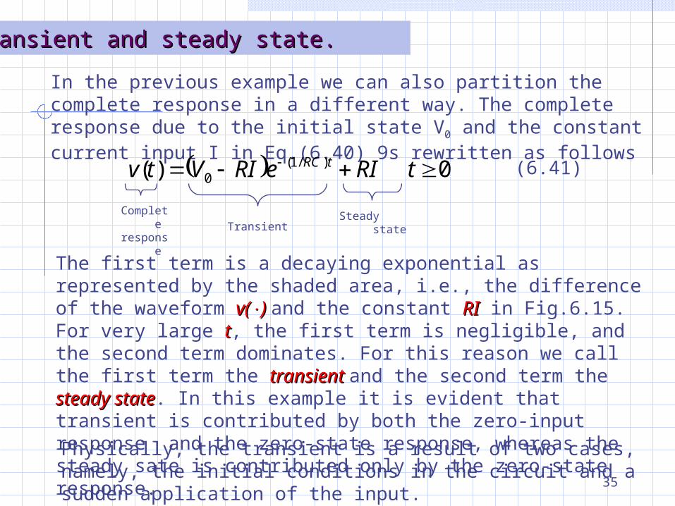
Transient and steady state.Transient and steady state.
In the previous example we can also partition the complete response in a different way. The complete response due to the initial state V0 and the constant current input I in Eq.(6.40) 9s rewritten as follows 0 )( )/1(
0 tRIeRIVtv tRC
Complete
response
Transient Steady state
(6.41)
The first term is a decaying exponential as represented by the shaded area, i.e., the difference of the waveform v(v() ) and the constant RIRI in Fig.6.15. For very large tt, the first term is negligible, and the second term dominates. For this reason we call the first term the transient transient and the second term the steady statesteady state. In this example it is evident that transient is contributed by both the zero-input response and the zero-state response, whereas the steady sate is contributed only by the zero-state response.Physically, the transient is a result of two cases, namely, the initial conditions in the circuit and a sudden application of the input.

36
The steady state is a result of only the input and has a waveform closely related to that of the input. If the input, for example, is a constant, the steady state response is also a constant; if the input is a sinusoid of angular frequency , the steady state response is also a sinusoid of the same frequency. In the example of sinusoid inpput, the input is )cos()( 11 tAtis ,the response has a steady state portion
)cos( 22 tA and a transient portion 1expcos 22 /RC)t) ((-φA
-1iis s
1F1F vv+
-
Fig.6.16 Exercise on steady state.
ExerciseExercise
The circuit shown in Fig. 6.16 contains 1-farad linear capacitor and a linear resistor with a negative resistance. When the current source is applied, it is in the zero state at time t=0t=0, so that for tt0, i0, iss=I=Immcoscost.t.
Calculate and sketch the response v. v.
Is there a sinusoidal steady state?

37
Circuits with Two Time ConstantsCircuits with Two Time Constants
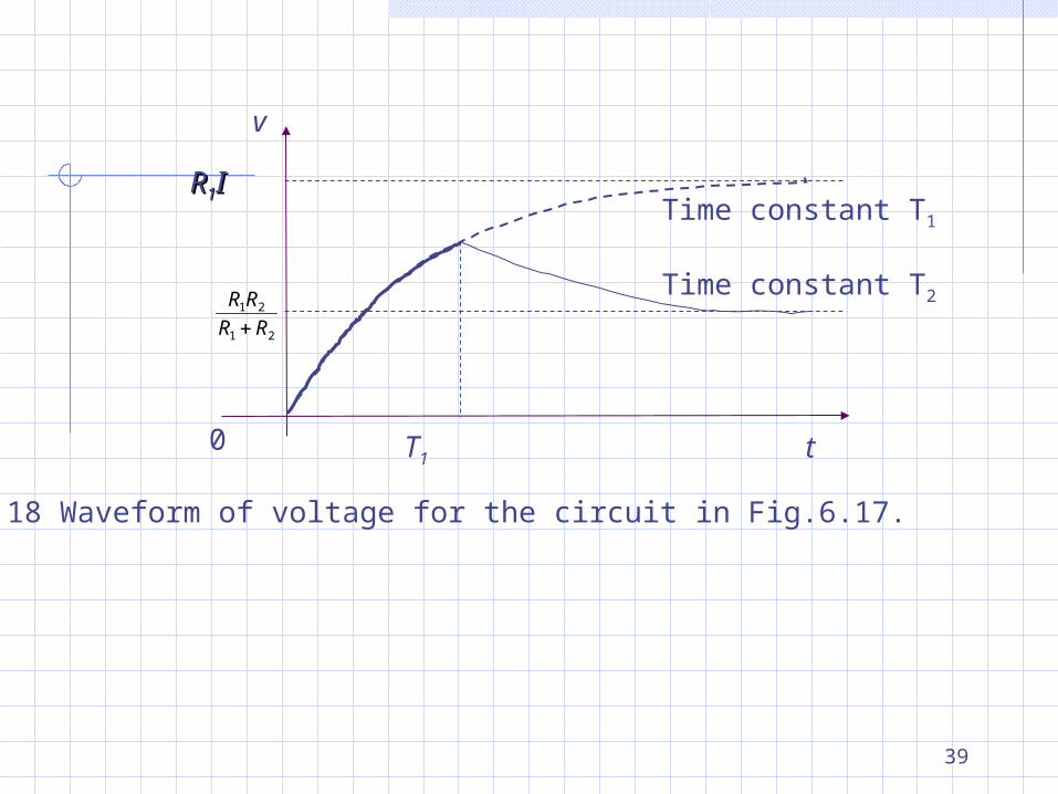
Problems involving the calculation of transients occur frequently in circuits with switches. Let us illustrate such a problem with the circuit shown in Fig. 6.17. Assume that the capacitor and resistors are linear and time invariant, and that the capacitor is initially uncharged. For t<0 t<0 switch kk11 is closed and switch kk22 is open. Switch k1is opened at t=0t=0 and thus connects the constant current source to the parallel RC circuit. The capacitor is gradually charged with the time constant TT11=R=R11CC11. Suppose that t=Tt=T11 ,switch kk22 is closed. The problem is to determine the voltage waveform across the capacitor for tt00.
R1kk11II
CC
k2
vv
+
-
R2
Fig.6.17 A simple transient problem. The switch kk11 is opened at t=0t=0; the switch kk22 is closed at t=Tt=T11=R=R11CC11.
We can divide the problem into to parts, the interval [0,T1] and the interval [T1, ]. First we determine the voltage in [0,T1] before switch k2 closes.

38
Since v(0)=0v(0)=0 by assumption, the zero-state response can be found immediately. Thus,
1
/1 0 )1(
0 0)(
1 TteIR
ttv
Tt
(6.42)
At t=Tt=T11
eIRTv
11)( 11
(6.43)
Which represents the initial condition for the second part of our problem. For t>Tt>T11 , since switch kk22 is closed we have a parallel combination of C, RC, R11 and RR22; the time constant is
21
212 RR
RRCT (6.44)
and the input is II. The complete response for this second part is, for ttTT11.
1/)(
21
21/)(1 )1(
11)( 2121 TteI
RR
RRe
eIRtv TTtTTt
(6.45)
39
v
t
Time constant T1
Time constant T2
0
21
21
RR
RR
RR11II
T1
Fig.6.18 Waveform of voltage for the circuit in Fig.6.17.
40
a
b
R
C
II
q C e t RC 1 /
t
q
RC 2RC
0
C
C
a
b+
- -
R+
I I
q
RC 2RC
0t
q C e t RC /
C
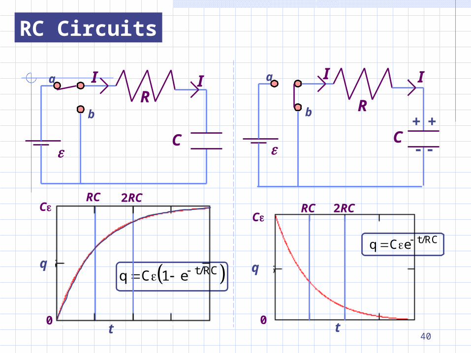
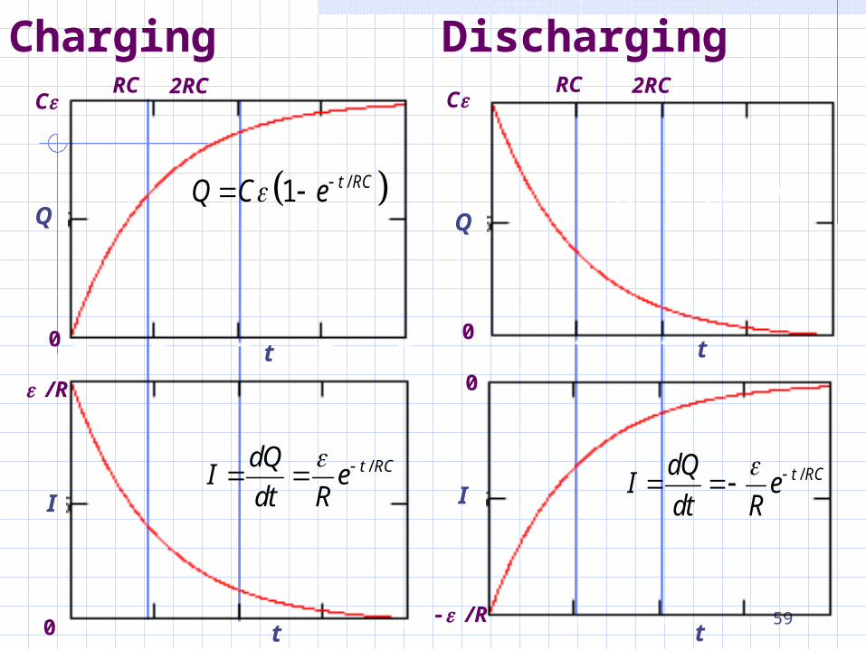
RC Circuits

41
• Calculate Charging of Capacitor through a Resistor
• Calculate Discharging of Capacitor through a Resistor
42
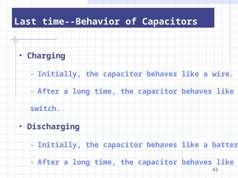
Last time--Behavior of Capacitors
• Charging
– Initially, the capacitor behaves like a wire.
– After a long time, the capacitor behaves like an open
switch.
• Discharging
– Initially, the capacitor behaves like a battery.
– After a long time, the capacitor behaves like a wire.

43
3) What is the voltage across the capacitor immediately after switch S1 is closed?
a) Vc = 0 b) Vc = E
c) Vc = 1/2 E
E
4) Find the voltage across the capacitor after the switch has beenclosed for a very long time.
a) Vc = 0 b) Vc = E
c) Vc = 1/2 E
The capacitor is initially uncharged, and the two switches are open.

44
Initially: Q = 0 VC = 0 I = E/(2R)
After a long time: VC = E Q = E C I = 0

45
6) After being closed a long time, switch 1 is opened and switch 2 is closed. What is the current through the right resistor immediately after the switch 2 is closed?
E
a) IR= 0
b) IR=E/(3R)
c) IR=E/(2R)
d) IR=E/R
Preflight 11:

46
After C is fully charged, S1 is opened and S2 is closed. Now, the battery and the resistor 2R are disconnected from the circuit. So we now have a different circuit.Since C is fully charged, VC = E. Initially, C acts like a battery, and I = VC/R.
47
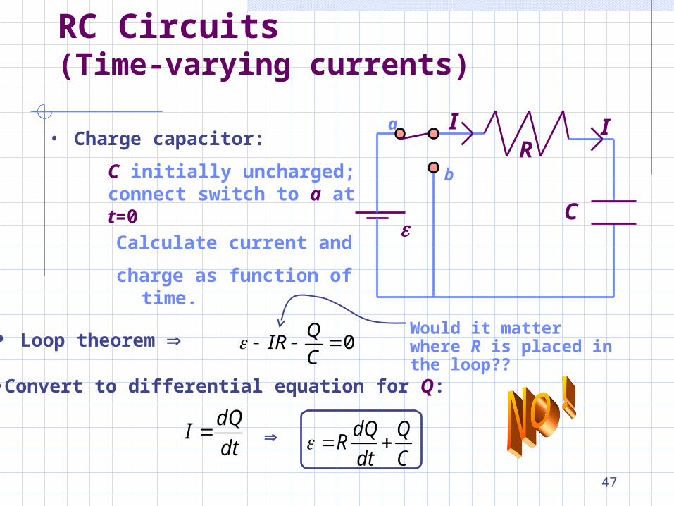
RC Circuits(Time-varying currents)
• Charge capacitor:
C initially uncharged; connect switch to a at t=0
• Loop theorem
•Convert to differential equation for Q:
a
b
R
C
II
Calculate current and
charge as function of time.
dt
dQI
C
Q
dt
dQR
Would it matter where R is placed in the loop??0
QIR
C

48
RC Circuits(Time-varying currents)
• Guess solution:
•Check that it is a solution:
00 Qt
CQt
Note that this “guess” incorporates the
boundary conditions:
a
b
R
C
II
dQ QR
dt C
Charge capacitor:
/ 1t RCdQC e
dt RC
)1(/ RC
tRCt ee
C
Q
dt
dQR !
(1 )t
RCQ C e

49
RC Circuits(Time-varying currents)
• Current is found from differentiation:
• Charge capacitor: a
b
R
C
II
/1 t RCQ C e
/t RCdQI e
dt R
Conclusion:
• Capacitor reaches its final charge(Q=C) exponentially with time constant = RC.
• Current decays from max (=/R) with same time constant.
50
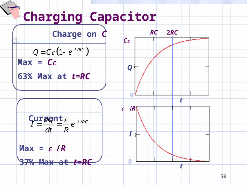
Charging Capacitor
Q
0
C Charge on C
Max = C
63% Max at t=RC
/1 t RCQ C e
t
RC 2RC
I
0t
R /t RCdQ
I edt R
Current
Max =/R
37% Max at t=RC
51
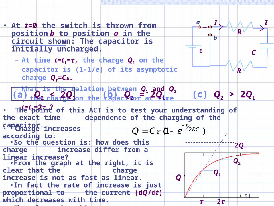
• At t=0 the switch is thrown from position b to position a in the circuit shown: The capacitor is initially uncharged.
– At time t=t1=, the charge Q1 on the capacitor is (1-1/e) of its asymptotic charge Qf=C.
– What is the relation between Q1 and Q2 , the
charge on the capacitor at time t=t2=2 ?
a
b
R
C
II
R
(a) Q2 < 2Q1 (b) Q2 = 2Q1 (c) Q2 > 2Q1
•From the graph at the right, it is clear that the charge increase is not as fast as linear.•In fact the rate of increase is just proportional
to the current (dQ/dt) which decreases with time.
•Therefore, Q2 < 2Q1.
Q
Q2
2Q1
Q1
• The point of this ACT is to test your understanding of the exact time dependence of the charging of the capacitor.
•So the question is: how does this charge increase differ from a linear increase?
)1( 2RCt
eCQ
• Charge increases according to:
52
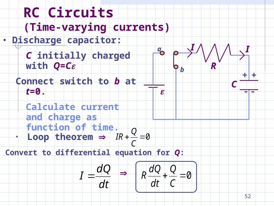
RC Circuits (Time-varying currents)
• Discharge capacitor:
C initially charged with Q=C
Connect switch to b at t=0.
Calculate current and charge as function of time.
• Convert to differential equation for Q:
C
a
b+ +
- -
R
I I
dt
dQI 0
C
Q
dt
dQR
0C
QIR• Loop theorem
53
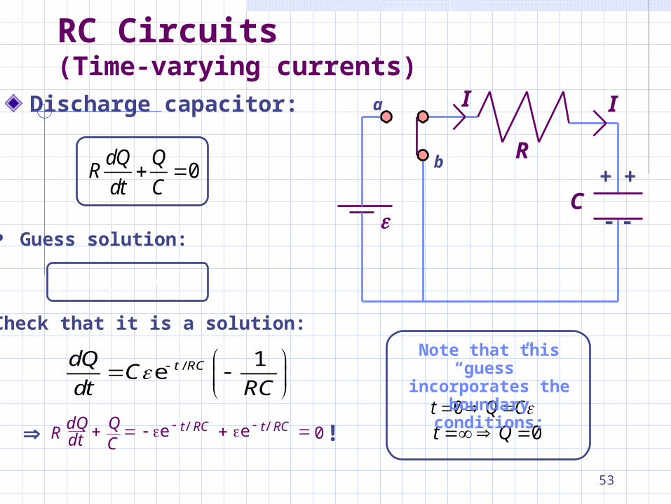
RC Circuits(Time-varying currents)
• Guess solution:
Q = Ce-t/RC
• Check that it is a solution:
/ 1e t RCdQ
Cdt RC
CQt 00 Qt
Note that this “guess” incorporates the
boundary conditions:
C
a
b+ +
- -
R0
dQ QR
dt C
I IDischarge capacitor:
!RdQdt
QC
e et RC t RC / / 0
54
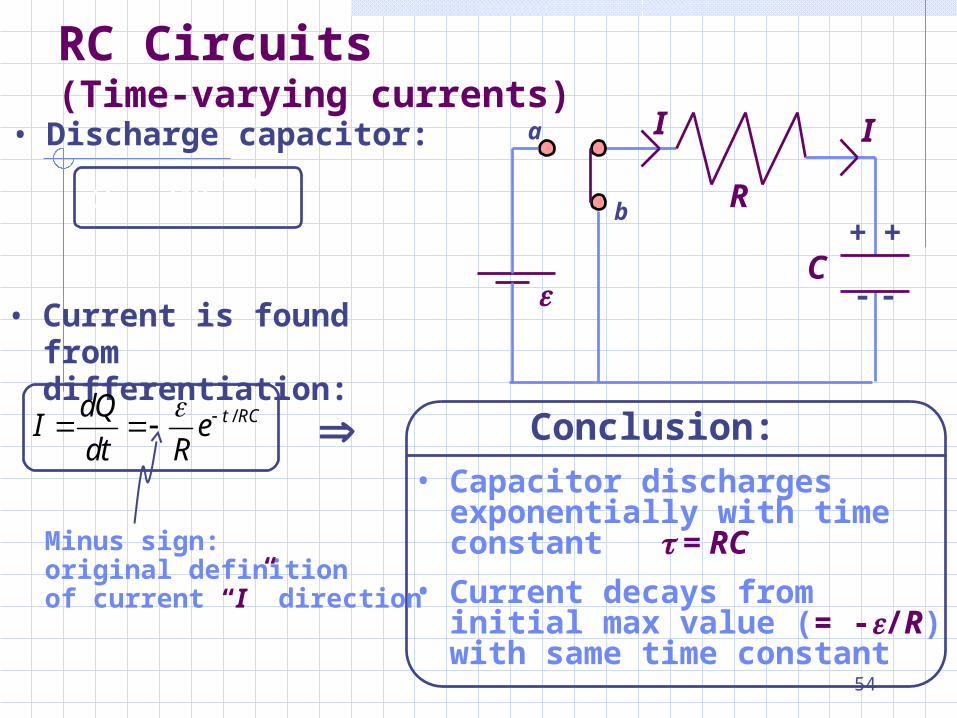
RC Circuits(Time-varying currents)
Conclusion: • Capacitor discharges
exponentially with time constant = RC
• Current decays from initial max value (= -/R) with same time constant
• Discharge capacitor: a
Q = Ce-t/RC
C
b+
- -
R+
I I
• Current is found from differentiation:
/t RCdQI e
dt R
Minus sign:original definitionof current “I” direction
55
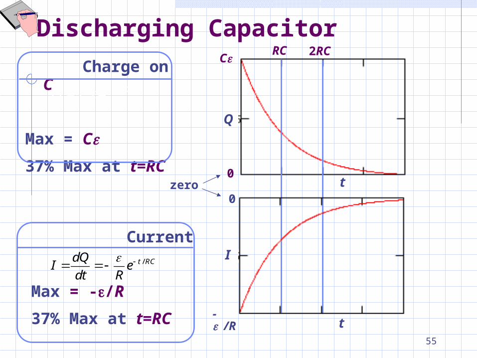
Discharging Capacitor
Charge on C
Max = C
37% Max at t=RC
Q = Ce-t/RC
/t RCdQ
I edt R
Current
Max = -/R
37% Max at t=RC
t
Q
0
C RC 2RC
0
-/R
I
t
zero
56
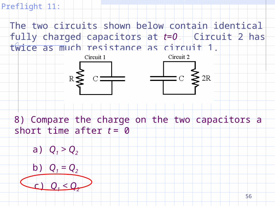
The two circuits shown below contain identical fully charged capacitors at t=0. Circuit 2 has twice as much resistance as circuit 1.
8) Compare the charge on the two capacitors a short time after t = 0
a) Q1 > Q2
b) Q1 = Q2
c) Q1 < Q2
Preflight 11:

57
Initially, the charges on the two capacitorsare the same. But the two circuits have different time constants:1 = RC and 2 = 2RC. Since 2 > 1 it takes circuit 2 longer to discharge its capacitor. Therefore, at any given time, the charge on capacitor is bigger than that on capacitor 1.
58
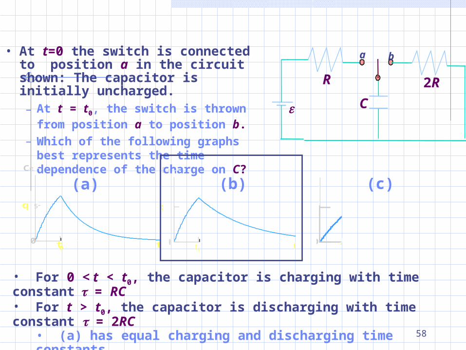
• At t=0 the switch is connected to position a in the circuit shown: The capacitor is initially uncharged.– At t = t0, the switch is thrown from
position a to position b.
– Which of the following graphs best represents the time dependence of the charge on C?
C
a b
R 2R
(a) (b) (c)
t
q
0
C
0 1 2 3 40
0.5
1
t/RC
Q f( )x
x
t0 t
q
0
C
0 1 2 3 40
0.5
1
t/RC
Q f ( )x
x
t 0 0 1 2 3 40
0.5
1
t/RCQ f ( )x
x
q
0
C
tt0
• For 0 < t < t0, the capacitor is charging with time constant = RC• For t > t0, the capacitor is discharging with time constant = 2RC
• (a) has equal charging and discharging time constants• (b) has a larger discharging t than a charging • (c) has a smaller discharging t than a charging
59
Charging DischargingRC 2RC
t
t
Q
0
C
I
0
/R
/1 t RCQ C e
/t RCdQI e
dt R
RC
t
2RC
0
-/R
I
t
Q
0
C
Q = C e -t/RC
/t RCdQI e
dt R

60
A very interesting RC circuitI1
I3
I2
R2C
R1
First consider the short and long term behavior of this circuit.
• Short term behavior:
Initially the capacitor acts like an ideal wire. Hence,
and
•Long term behavior:
Exercise for the student!!

61
10) Find the current through R1 after the switch has been closed for a long time.
a) I1 = 0 b) I1 = E/R1 c) I1 = E/(R1+ R2)
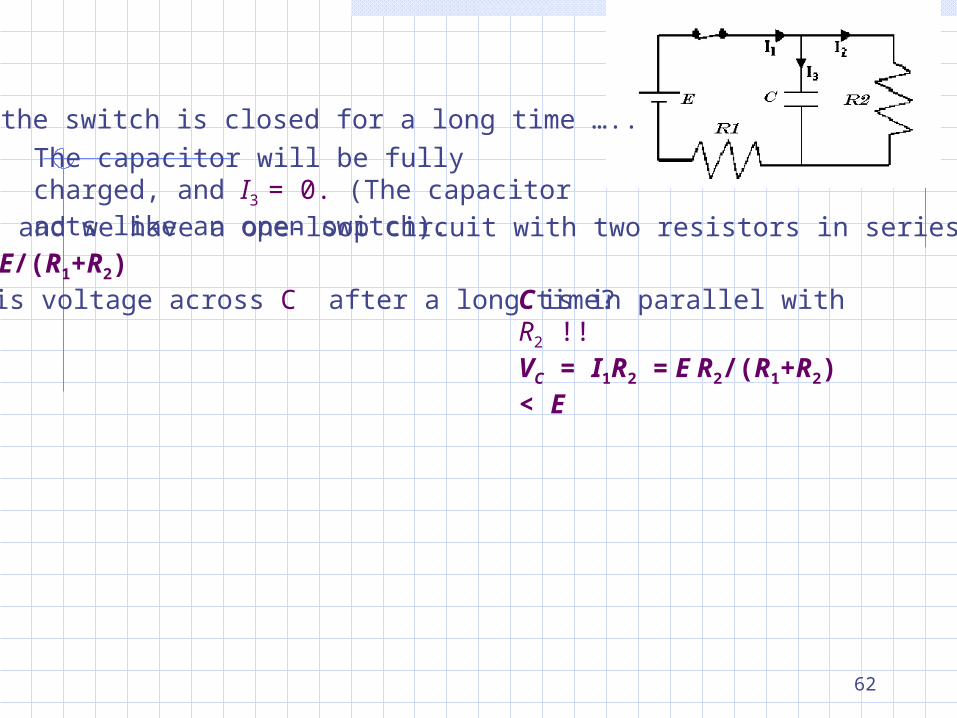
The circuit below contains a battery, a switch, a capacitor and two resistors
Preflight 11:
62
After the switch is closed for a long time …..
The capacitor will be fully charged, and I3 = 0. (The capacitor acts like an open switch).So, I1 = I2, and we have a one-loop circuit with two resistors in series,hence I1 = E/(R1+R2)What is voltage across C after a long time? C is in parallel with R2 !!
VC = I1R2 = E R2/(R1+R2) < E

63
Very interesting RC circuit continued
I1
I3
I2
R2C
R1
Loop 1
Loop 2
• Node:
Loop 1: 1 1 0Q
I RC
Loop 2: 2 2 1 1 0I R I R
321 III
Eliminate I1 in L1 and L2 using Node equation:
Loop 1: 1 2 0Q dQ
R IC dt
Loop 2: 2 2 1 2 0dQ
I R R Idt
eliminate I2 from this
Final differential eqn:1 1 2
1 2
dQ Q
R dt R RC
R R

64
Very interesting RC circuit continued
• Try solution of the form:
– and plug into ODE to get parameters A and τ
Final differential eqn:
1
21
21 RC
RRRR
Q
dt
dQ
time constant: parallel combination
of R1 and R2
/1)( teAtQ
Obtain results that agree with initial and final conditions:
CRR
RR
21
212
1 2
RA C
R R
I1
I3
I2
R2C
R1
Loop 1
Loop 2
65
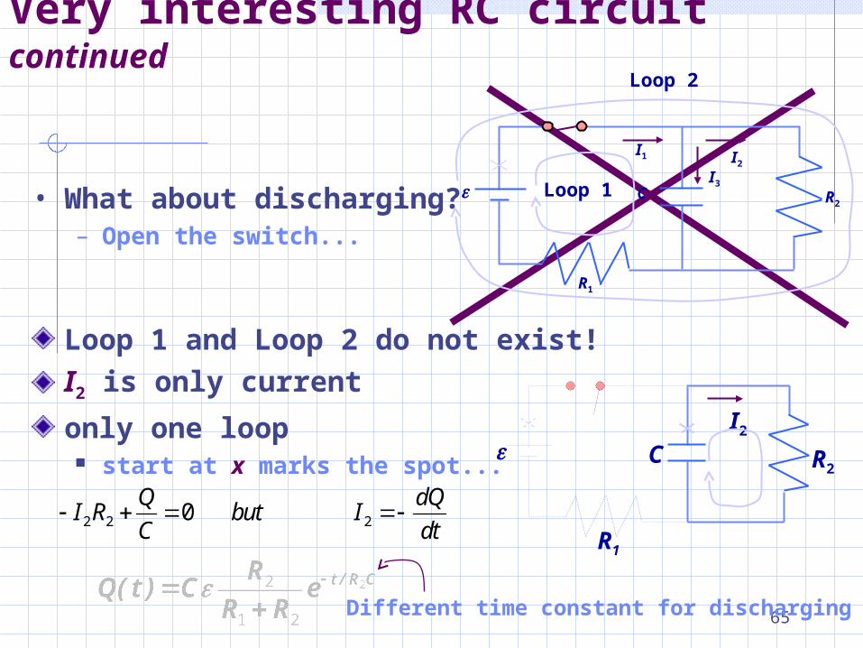
Very interesting RC circuit continued
• What about discharging?– Open the switch...
Loop 1 and Loop 2 do not exist!
I2 is only current
only one loop start at x marks the spot...
I2 R2
C
R1
2 2 20Q dQ
I R but IC dt
Different time constant for discharging
I1
I3
I2
R2C
R1
Loop 1
Loop 2

66
• Kirchoff’s Laws apply to time dependent circuits they give differential equations!
• Exponential solutions– from form of differential equation
• time constant = RC
– what R, what C?? You must analyze the problem!
• series RC charging solution
• series RC discharging solution Q = C e -t/RC
/1 e t RCQ C
Q = C e -t/RC