1 introduction to graph mining sangameshwar patil systems research lab trddc, tcs, pune

1

Introduction to Graph Mining

Sangameshwar PatilSystems Research Lab

TRDDC, TCS, Pune

2

Outline

• Motivation– Graphs as a modeling tool– Graph mining

• Graph Theory: basic terminology • Important problems in graph mining• FSG: Frequent Subgraph Mining Algorithm

3

Motivation

• Graphs are very useful for modeling variety of entities and their inter-relationships

– Internet / computer networks• Vertices: computers/routers• Edges: communication links

– WWW• Vertices: webpages• Edges: hyperlinks

– Chemical molecules• Vertices: atoms• Edges: chem. Bonds

– Social networks (Facebook, Orkut, LinkedIn)• Vertices: persons• Edges: friendship

– Citation/co-authorship network – Disease transmission– Transport network (airline/rail/shipping)– Many more…

4

Motivation: Graph Mining

• What are the distinguishing characteristics of these graphs?

• When can we say two graphs are similar?• Are there any patterns in these graphs?• How can you tell an abnormal social network

from a normal one? • How do these graph evolve over time?• Can we generate synthetic, but realistic graphs?

– Model evolution of Internet?

• …

5

Terminology-I

• A graph G(V,E) is made of two sets– V: set of vertices– E: set of edges

• Assume undirected, labeled graphs– Lv: set of vertex labels

– LE: set of edge labels

• Labels need not be unique – e.g. element names in a molecule

6

Terminology-II

• A graph is said to be connected if there is path between every pair of vertices

• A graph Gs (Vs, Es) is a subgraph of another graph G(V, E) iff – Vs is subset of V and Es is subset of E

• Two graphs G1(V1, E1) and G2(V2, E2) are isomorphic if they are topologically identical– There is a mapping from V1 to V2 such that each edge

in E1 is mapped to a single edge in E2 and vice-versa

7

Example of Graph Isomorphism

ƒ(a ) = 1

ƒ(b ) = 6

ƒ(c ) = 8

ƒ(d ) = 3

ƒ(g ) = 5

ƒ(h ) = 2

ƒ(i ) = 4

ƒ(j ) = 7

8

Terminology-III: Subgraph isomorphism problem

• Given two graphs G1(V1, E1) and G2(V2, E2): find an isomorphism between G2 and a subgraph of G1

– There is a mapping from V1 to V2 such that each edge in E1 is mapped to a single edge in E2 and vice-versa

• NP-complete problem– Reduction from max-clique or hamiltonian cycle

problem

9

Need for graph isomorphism

• Chemoinformatics– drug discovery (~ 1060 molecules ?)

• Electronic Design Automation (EDA)– designing and producing electronic systems ranging

from PCBs to integrated circuits

• Image Processing• Data Centers / Large IT Systems

10

Other applications of graph patterns

• Program control flow analysis– Detection of malware/virus

• Network intrusion detection• Anomaly detection• Classifying chemical compounds• Graph compression• Mining XML structures• …

11

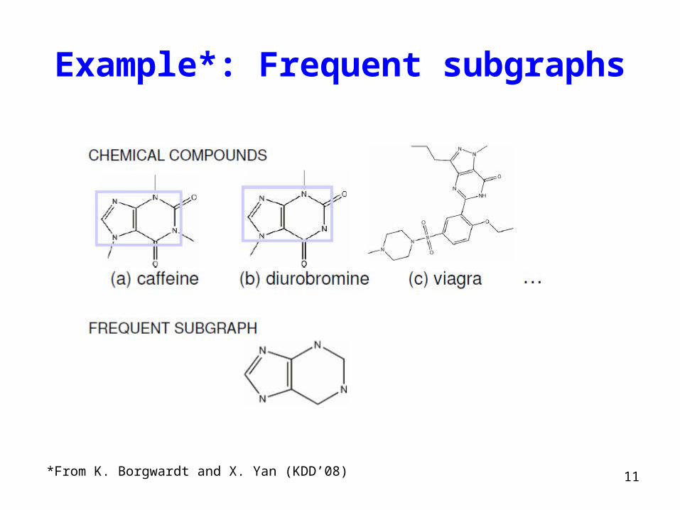
Example*: Frequent subgraphs

*From K. Borgwardt and X. Yan (KDD’08)

12

Questions ?

13

An Efficient Algorithm for Discovering Frequent Sub-

graphs

IEEE ToKDE 2004 paper

by

Kumarochi & Karypis

14

Outline

• Motivation / applications• Problem definition• Recap of Apriori algorithm• FSG: Frequent Subgraph Mining Algorithm

– Candidate generation– Frequency counting– Canonical labeling

16

Outline

• Motivation / applications• Problem definition

– Complexity class GI

• Recap of Apriori algorithm• FSG: Frequent Subgraph Mining Algorithm


17

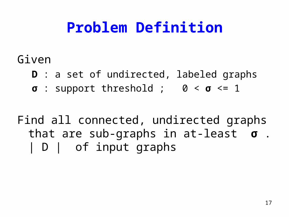
Problem Definition

Given D : a set of undirected, labeled graphs

σ : support threshold ; 0 < σ <= 1

Find all connected, undirected graphs that are sub-graphs in at-least σ . | D | of input graphs

18

Complexity

• Sub-graph isomorphism– Known to be NP-complete

• Graph Isomorphism (GI)– Ambiguity about exact location of GI in conventional complexity

classes • Known to be in NP• But is not known to be in P or NP-C• (factoring is another such problem)

– A class in its own• Complexity class GI • GI-hard• GI-complete

19

Outline



20

Apriori-algorithm: Frequent Itemsets

Ck: Candidate itemset of size k

Lk: frequent itemset of size kFrequent: count >= min_support

• Find frequent set Lk−1.• Join Step

– Ck is generated by joining Lk−1 with itself

• Prune Step – Any (k−1)-itemset that is not frequent cannot be a

subset of a frequent k -itemset, hence should be removed.

21

Apriori: Example

Set of transactions : { {1,2,3,4}, {2,3,4}, {2,3}, {1,2,4}, {1,2,3,4}, {2,4} }

min_support: 3

L1 C2 L2L3

{1,2,3} and {1,3,4} were pruned as {1,3} is not frequent.

{1,2,3,4} not generated since {1,2,3} is not frequent. Hence algo terminates.

22

Outline



23

FSG: Frequent Subgraph Discovery Algo.

• ToKDE 2004– Updated version of ICDM 2001 paper by same authors

• Follows level-by-level structure of Apriori• Key elements for FSG’s computational

scalability– Improved candidate generation scheme– Use of TID-list approach for frequency counting– Efficient canonical labeling algorithm

24

FSG: Basic Flow of the Algo.

• Enumerate all single and double-edge subgraphs

• Repeat– Generate all candidate subgraphs of size (k+1) from

size-k subgraphs– Count frequency of each candidate– Prune subgraphs which don’t satisfy support

constraint

Until (no frequent subgraphs at (k+1) )

25

Outline



26

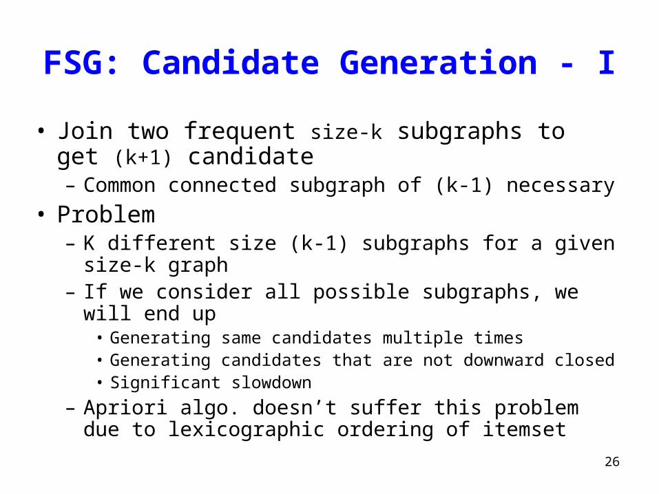
FSG: Candidate Generation - I

• Join two frequent size-k subgraphs to get (k+1) candidate– Common connected subgraph of (k-1) necessary

• Problem– K different size (k-1) subgraphs for a given size-k

graph– If we consider all possible subgraphs, we will end up

• Generating same candidates multiple times• Generating candidates that are not downward closed• Significant slowdown

– Apriori algo. doesn’t suffer this problem due to lexicographic ordering of itemset

27

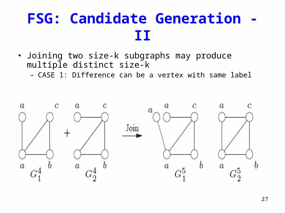
FSG: Candidate Generation - II

• Joining two size-k subgraphs may produce multiple distinct size-k – CASE 1: Difference can be a vertex with same label

28

FSG: Candidate Generation - III

• CASE 2: Primary subgraph itself may have multiple automorphisms

• CASE 3: In addition to joining two different k-graphs, FSG also needs to perform self-join

29

FSG: Candidate Generation Scheme

• For each frequent size-k subgraph Fi , define

primary subgraphs: P(Fi) = {Hi,1 , Hi,2}

• Hi,1 , Hi,2 : two (k-1) subgraphs of Fi with smallest and second smallest canonical label

• FSG will join two frequent subgraphs Fi and Fj iff

P(Fi) ∩ P(Fj) ≠ Φ

This approach correctly generates all valid candidates and leads to significant performance improvement over the ICDM 2001 paper

30

Outline



31

FSG: Frequency Counting

• Naïve way– Subgraph isomorphism check for each candidate against each graph

transaction in database– Computationally expensive and prohibitive for large datasets

• FSG uses transaction identifier (TID) lists– For each frequent subgraph, keep a list of TID that support it

• To compute frequency of Gk+1 – Intersection of TID list of its subgraphs– If size of intersection < min_support,

• prune Gk+1 – Else

• Subgraph isomorphism check only for graphs in the intersection• Advantages

– FSG is able to prune candidates without subgraph isomorphism– For large datasets, only those graphs which may potentially contain the

candidate are checked

32

Outline



33

Canonical label of graph

• Lexicographically largest (or smallest) string obtained by concatenating upper triangular entries of adj. matrix (after symmetric permutation)

• Uniquely identifies a graph and its isomorphs– Two isomorphic graphs will get same canonical label

34

Use of canonical label

• FSG uses canonical labeling to– Eliminate duplicate candidates– Check if a particular pattern satisfies the downward

closure property

• Existing schemes don’t consider edge-labels– Hence unusable for FSG as-is

• Naïve approach for finding out canonical label is O( |v| !)– Impractical even for moderate size graphs

35

FSG: canonical labeling

• Vertex invariants– Inherent properties of vertices that don’t change across

isomorphic mappings– E.g. degree or label of a vertex

• Use vertex invariants to partition vertices of a graph into equivalent classes

• If vertex invariants cause m partitions of V containing p1, p2, …, pm vertices respectively, then number of different permutations for canonical labeling

π (pi !) ; i = 1, 2, …, m

which can be significantly smaller than |V| ! permutations

36

FSG canonical label: vertex invariant - I

• Partition based on vertex degrees and labels

Example: number of permutations reqd = 1 ! x 2! x 1! = 2Instead of 4! = 24

37

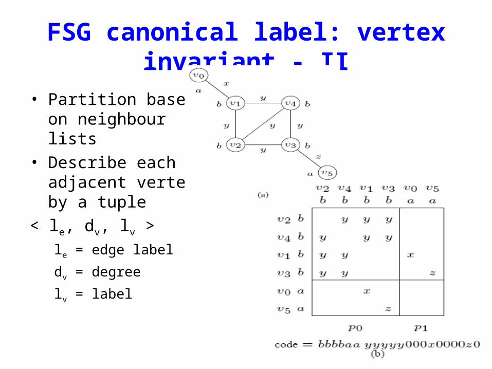
FSG canonical label: vertex invariant - II

• Partition based on neighbour lists

• Describe each adjacent vertex by a tuple

< le, dv, lv >

le = edge label

dv = degree

lv = label

38

FSG canonical label: vertex invariant - II

• Two vertices in same partition iff their nbr. lists are same• Example: only 2! Permutations instead of 4! x 2!

39

FSG canonical label: vertex invariant - III

• Iterative partitioning• Different way of

building nbr. list • Use pair <pv, le> to

denote adjacent vertex– pv = partition number of

adj. vertex c– le = edge label

40


Iter 1: degree based partitioning

41


Nbr. List of v1 is different from v0, v2. Hence new partition introduced.

Renumber partitions and update nbr. lists. Now v5 is different.

42


43

Next steps

• What are possible applications that you can think of?– Chemistry– Biology

• We have only looked at “frequent subgraphs”– What are other measures for similarity between two graphs?– What graph properties do you think would be useful?– Can we do better if we impose restrictions on subgraph?

• Frequent sub-trees• Frequent sequences• Frequent approximate sequences

• Properties of massive graphs (e.g. Internet)– Power law (zipf distribution)– How do they evolve?– Small-world phenomenon (6 hops of separation, kevin beacon number)

44

Questions ?

Thanks

1 introduction to graph mining sangameshwar patil systems research lab trddc, tcs, pune

Documents

vertices e

graph g s v s

graph gv

subset of e

graphs g

e iff v s

graph mining fsg

pune slide