1 intr - yale university · alba, nic k dero os, mireia jofre-bonet, jennifer murdo c k, katja...
TRANSCRIPT

Rational Addiction and Rational Cessation: A
Dynamic Structural Model of Cigarette
consumption�
by Eugene Choo,
Yale University y
20th November 2000
Comments welcome.
Abstract
Much of the existing empirical literature on smoking addiction takes a re-
duced form approach. While interesting and simple to implement, this approach
only allows a restricted range of possible policy experiments, usually in the form
of price changes. This paper builds and estimates a dynamic structural model of
rational addiction and cessation using longitudinal data from a smoking cessation
study. A new methodological framework is presented that explains quitting and
smoking behavior, and allows interesting and pertinent policy experiments that
existing models have diÆculty analyzing. This model allows us to consider the ef-
fects of regulating the level of nicotine in cigarettes, subsidizing quitting behavior,
�nding a cure for lung cancer as well as temporal changes in prices. It explicitly
models the unobserved addiction and health process. Using additional data from
medical studies, I exogenously identify the health generating process and incorpo-
rate it into the model. The paper shows that the addition of health e�ects into a
model of rational addiction is important in explaining smoking dynamics.
�I am grateful to my advisors, Steve Berry and Ariel Pakes for guidance and advice, John Rust, ChrisTimmins, Pat Bayer, G�unter Hitsch, and Oleg Melnikov for immeasurably helpful discussions, supportand encouragements. I also thank Tracy Falba, Nick DeRoos, Mireia Jofre-Bonet, Jennifer Murdock,Katja Seim, Nikolay Moshkin, Martin Pesendorfer, the seminar participants at Yale and Harvard forhelpful comments. I am indebted to William Lyn at the National Cancer Institute who graciouslyprovided the COMMIT study data. Any errors and ommissions are my own.
yAuthor's contact information: email: [email protected], Phone: (203) 432 3567, Fax: (203)432 6323, Homepage: http://www.econ.yale.edu/�echoo
1

1 Introduction and Motivation
There is a long history of empirical research modeling cigarette addiction. Much of
the existing empirical literature takes a reduced form approach that attempts to explain
observed smoking and quitting behavior using past (and future1) behavior, prices, and
demographic characteristics. While interesting and easy to implement, this approach
has not been able to look at some of the policy experiments that this paper considers.
This is an empirical study of smoking using a model of rational addiction. It presents a
framework that explains smoking and quitting behavior, and allows us to consider a va-
riety of policy experiments that the existing empirical literature has diÆculty analyzing.
More importantly, it provides a practical and intuitive way of incorporating health when
modeling smoking addiction. While there has been much medical evidence showing the
negative health e�ects of smoking and the health bene�ts of smoking cessation,2 formal
empirical modeling of the dynamic health process and the way it interacts with smoking
and quitting behavior has not been attempted. This is largely because of the diÆculty
of observing the health status of individuals. The data used in this paper have similar
limitations. This paper introduces a stochastic health process using external medical
data and shows that health e�ects are important in explaining quitting behavior. I �rst
discuss the limitations of the existing literature and then explain what this paper has
to o�er.
The traditional reduced form approach of modeling cigarette consumption estimates
a generalized linear model and uses it to evaluate the e�ectiveness of excise tax policies3
or other regulatory policies4 on smoking. This approach typically requires either individ-
ual or aggregate level data on observed consumers' responses to policy changes in order
to estimate an empirical relationship between individuals' behavior as a function of the
policy instrument of interest. This methodology only allows us to evaluate the e�ects of
policy experiments that have already been conducted. As such, these models will have
1In the existing empirical rational addiction literature including Chaloupka (1991) and Becker, Gross-man, and Murphy (1994), lead consumption and prices are also included as regressors in the linearmodel.
2Examples of references include US Dept. of Health of Human Services (1989) and (1990).3Examples include Lewit and Coate (1982), Wasserman, Manning, Newhouse, and Winkler (1991),Becker, Grossman, and Murphy (1994) and Chaloupka (1991).
4Some papers that analyze policies other than prices include Hu, Sung, and Keeler (1995), Barnett, Hu,Sung, and Keeler (1995), which looked at the e�ectiveness of antismoking media policies in California,and Chaloupka and Wechsler (June, 1997), which looked at control policies on youth smoking.
2

diÆculty analyzing policy experiments that have not yet been conducted. Examples of
these policy experiments include analyzing the impact of regulating the level of nicotine
in cigarettes, the e�ects of subsidizing quitting behavior, and the impact of �nding a cure
for lung cancer. Even though these policy experiments have never been conducted, they
remain options for both state and federal regulators interested in regulating smoking.
Second, traditional models have not focused on explaining the patterns of smok-
ing and quitting behavior observed in data. Empirical evidence suggests that quitting
usually occurs `cold turkey', with many quitters often relapsing to the level they were
smoking before they quit for good. Smokers who continue smoking smoke a relatively
stable number of cigarettes. Traditional models have diÆculty generating and explain-
ing these extreme behaviors: small changes in consumption amongst continuing smokers
and large discrete changes among quitters. The attractive feature about a generalized
linear model is that the error term can take any value on the real line. Hence, it can be
�tted to all observed behaviors, even though upon simulation these models do poorly at
replicating behaviors seen in data.
The morbidity associated with smoking addiction has been well documented. Evi-
dence suggests that many smokers begin to experience the negative consequences from a
lifetime of smoking when they reach middle-age (Behrman, Sickles, and Taubman (1990)
and (2000)). Studies have also shown that health concerns and health events become im-
portant initiators of smoking cessation among smokers of this age group (Falba (2000)).
While much is known about the health consequences of cigarette smoking, there has been
little formal empirical modeling of the health process and quantifying its importance in
observed quitting dynamics.5
The empirical rational addiction literature (like Chaloupka (1991) and others that
follow) often uses the in uential model of Becker and Murphy (1988) as the theoretical
base for the empirical application. These papers make a functional form assumption on
the individual's utility function that generalizes the Euler equation to a simple linear
model. This simpli�cation allows the implications of the rational addiction model to be
tested in an empirically tractable way. However, these derivations usually ignore the
binding constraint that quitting behavior poses on the �rst order condition of a utility
maximizing individual. As such, the empirical moment conditions taken to data no
5Notable references that looks at the importance of health in smoking cessation include Jones (1994)and Hu, Ren, Keeler, and Bartlett (1995).
3

longer accurately represent the �rst order conditions implied by the rational addiction
model. Further more, these papers do not try to estimate the structural parameters that
are of signi�cant policy interest. These include the parameters of the utility function and
those that govern the evolution of the state variables.6 See Section 7.1 of the Appendix
for an example of the derivation of the Euler equation for a habit formation model that
correctly account for the binding constraint on the choice set.
This paper attempts to remedy the aforementioned limitations. It develops a dy-
namic structural model of rational addiction and cessation, and estimates it using longi-
tudinal data from a National Cancer Institute (NCI) study into smoking cessation. The
paper explicitly models the individuals smoking and quitting behavior using a utility
maximising framework with uncertainty while taking into account the e�ects the indi-
vidual's behavior has on the addiction and health process. It expicitly puts a dynamic
structure on the stochastic addiction and health process.7 I make structural assump-
tions about the decision making process, the beliefs of the individual, the nature of the
stochastic addiction and health process, and the manner in which it a�ects the individ-
ual's well-being. These assumptions drive the estimation of the structural parameters.
Having these parameter estimates provides us with additional degree of freedom when
looking policy experiments.
This paper has two main goals. The �rst is to present a framework that allows us to
consider a larger variety of experiments than currently possible. This is accomplished
by providing a structural model of rational addiction and cessation that can be taken
to data. It is the structural parameters of the model that allow us to consider the new
variety of policy experiments that traditional models have diÆculty analyzing. This
paper allows us to consider, for example, the e�ects of regulating the level of nicotine
in cigarettes, subsidizing quitting behavior, �nding a cure for lung cancer, and temporal
changes in prices.
6The Euler equation that accounts for this choice constraint will have to assume that the smoker whoquits will resume smoking sometime in the future in order to arrive at a compensating change neededfor the �rst order conditions to hold for an optimizing individual. Hence, an implicit assumptionunderlying the moment condition approach is that a smoker would never permanently quit.
7Many addictions typically involve an unobserved addiction process that a�ects current behavior andbehaviors in the future. Putting a dynamic structure on how this unobserved state evolves is importantwhen making long run predictions of policy changes. A policy change, like a price increase, will causesmokers to alter their short-run behavior. These short run behavioral changes will a�ect the way theaddiction process evolves. Existing models that do not explicitly model the changes to this unobservedaddiction process may give misleading long run predictions, even for policy experiments for which thereare data.
4

The second goal is to provide a model that explains smoking and quitting behav-
ior. I show that the speci�cation of a simple habit formation model with the stochastic
addiction stock being the only unobserved state, is not suÆciently rich to explain the
dynamics observed in data. Instead, a model that incorporates a health process is shown
to be able to explain the discrete jumps associated with cold turkey quits and relapse.
This health process, which incorporates the morbidity of smoking addiction, is identi�ed
using data from an external medical study (into diseases associated with tobacco use).
I show through simulation that the addition of health e�ects to a simple habit forma-
tion/rational addiction model is important in explaining smoking and quitting dynamics.
Finally, the framework presented also has applications outside cigarette addiction.
The natural extension would be in modeling other forms of addiction (like gambling, al-
cohol and drug addiction, etc.) or clinical experiments involving an addiction process.8
This model can also be extended to situations where individuals or �rms repeatedly
engage in an activity that has dynamic consequences. Possible applications in empirical
industrial organization include modeling repeated retail purchases of a consumer good
with habit or taste formation, or a �rm's advertising or investment expenditure con-
tributing to an unobserved state like goodwill9 or �rm's productivity.
The paper is organized as follow. Section 2 provides a brief review of related litera-
ture. A description and preliminary analysis of the data is provided in section 3. Section
4 de�nes the model and provides a brief outline of the intuition behind its setup. Monte
Carlo simulation is presented in Section 5 and Section 6 concludes.
2 Existing Literature
Economists have long been puzzled by the many inconsistencies of addiction. The
main distinguishing feature being individuals repeatedly engaging in an activity that
provides immediate gratication and pleasure, while knowingly ignoring its adverse con-
sequences in the future. Non-addicts do not face this impulsive need and are able to
stay away from these activities. Economic models that analyze addiction fall into two
8The current speci�cation of the model assumes that addiction only contributes to a reinforcement
e�ect, which is not a reasonable approximation of all addictions. This is something I intend to relaxin future extensions of this research.
9A recent empirical industrial organization paper by Hitsch (2000) has this feature in his model.
5

broad categories.
One response has been to ignore the rational choice framework and develop models of
irrational behavior. An exhaustive review on this sizeable body of theoretical literature
is beyond the scope of this paper.10 Some themes emphasized in this literature include
the compulsiveness of addictive consumption (Shefrin (1984)), self control and myopia
(e.g. Thaler and Shefrin (1981) and O'Donoghue and Rabin (1999)), and timing incon-
sistencies ( Akerlof (1991) and Ainslie and Haslam (1992)). For example, Ainslie and
Haslam (1992) provide evidence of timing inconsistencies, and consider the implications
if time discounting is hyperbolic rather than the exponential as assumed in standard
rational choice theory. Thaler and Shefrin (1981) and Shefrin (1984) explain complu-
siveness and myopia by allowing the individual to have multiple sets of preferences that
may be con icting. Identifying and testing the behavioral predictions of these models
has been restricted to experimental studies.
The other response is to explain these apparently irrational behaviors using the stan-
dard assumptions of the rational choice framework. The seminal paper of Stigler and
Becker (1977) and Becker and Murphy (1988), argued that addictive consumption is
consistent with rational, forward looking, utility maximizing behavior. Becker and Mur-
phy (1988) relax the intertemporal separability assumption of utility by allowing current
consumption to add to a consumption capital that lowers overall utility, while increasing
the marginal utility from the good in the future. The model explains the reinforcement,
tolerance, and withdrawal features of addiction and is able to motivate binging and
`cold turkey' quitting behavior. This model has been praised as well as criticized for
being inconsistent with observed addictive behavior. A number of papers have intro-
duced modi�cations to this model to arrive at more realistic predictions. Dockner and
Feichtinger (1993) allow for a more general addiction process where the addictive good
accumulates to two di�erent stocks of consumption capital. Their modi�cation allows
for a variety of cyclical consumption pro�les over time. Orphanides and Zervos (1995) al-
low for individual uncertainty about the addictive nature of the consumption good. The
authors explain rational addiction in terms of learning through experimentation. Their
followup paper, Orphanides and Zervos (1998), allow for state dependent discount rates.
Introducing this general discount rate reconciles myopic behavior amongst addicts and
10Rabin (1998) provides a nice discussion of many of the ideas in behavioral economics, not necessarilyrelated to addiction.
6

optimizing far-sighted behavior amongst non-addicts within the rational choice frame-
work.
A number of empirical papers have taken Becker and Murphy's (1988) rational ad-
diction model to data. Papers like Chaloupka (1991) and Becker, Grossman, and Mur-
phy (1994) use a discrete time version of Becker and Murphy's (1988) model with the
assumption that the utility function takes a quadratic form. This linearizes the �rst
order condition and can be estimated using a general method of moments procedure.
Chaloupka (1991) applies this to individual level data to test the implications of the ra-
tional model. As mentioned earlier, this and subsequent paper using the Euler condition
ignore the binding constraints quitting behavior places on the choice set. Furthermore,
these papers do not try to estimate the structural parameters and have not focused on
trying to explain actual smoking and quitting behavior.11
A growing body of empirical papers have looked at the e�ects of health on smoking
and quitting behavior. Jones (1994) uses survey data from Britain's Health and Lifestyle
Survey to investigate the e�ects that various measures of health status, social interaction
and addiction have on the likelihood that a smoker attempts and succeeds at quitting.
Using current health status to proxy for past health, he �nds the interesting result that
poor health is associated with a lower likelihood of cessation, while smokers with long
standing disability or illness have a higher likelihood of quitting. Using data from the
Health and Retirement Study (HRS), Falba (2000) looks at the e�ects that a new diag-
nosis of an acute illness and decline in functionality have on smoking cessation in middle
aged married couples. The author �nds that the new diagnosis of an acute or chronic
illness is a strong motivator for smoking cessation. Other studies include Wray, Her-
zog, Willis, and Wallace (1998) that looked at the e�ects heart attack has on continued
smoking, and Smith et al. (2000) uses the HRS panel to assess how health events change
the life expectations of smoker and non-smokers. These papers highlight the importance
of morbidity in determining quitting behavior amongst middle-aged smokers.12
As a further example of the importance of health status in smoking and quitting
decisions, participants of the COMMIT study, (used in this paper and to be described
in Section 3) were asked to give their reasons for attempting to quit in the �nal inter-
11Section 7.1 of the Appendix provides a derivation of the Euler condition that correctly re ect thebounded choice set.
12Quitting has been posed as either a curative or preventive measure taken by a smoker when faced withthe prospect of increase health problems in the future from continual smoking. See Jones (1994).
7

view. The results, taken from another study using the same data are shown in Table 2.
The most common reasons given were concern over health and the expense associated
with smoking. In this paper, I extend this idea further by formally putting a dynamic
structure to the health process and integrating this into a rational choice framework.
Insert Table 2 here. Note that some tables are left to the end of the paper.
3 The Data
This section provides a brief description of the data sets used in this paper. Some de-
tails on the sampling process of this study have been left to Section 7.2 of the Appendix.
The main longitudinal dataset comes from a NCI funded project entitled `The Com-
munity Intervention Trial for Smoking Cessation' (COMMIT hereafter). This project
was created to investigate the e�ectiveness of community wide interventions in help-
ing smokers achieve and maintain long-term smoking cessation. The project began in
1989 and lasted till 1993. It was conducted in 11 matched pairs of communities, 10
pairs in the US, and the remaining pair in Canada. A community is broadly de�ned to
include a portion of a major metropolitan area or two small cities in the same geograph-
ical location. There is a distinct geographical boundary separating these communities
to ensure independence of intervention activities and minimize contamination. These
selected communities were matched for general socio-demographic characteristics, like
population size, demographic pro�le, (such as age and income distribution, ethnicity),
smoking prevalence rate, access to intervention channels, etc. Table 3.1 shows some
general statistics on the communities enrolled under COMMIT. One of the communi-
ties in each pair was randomized into an intervention group. The intervention activities
were organized around four task forces that include health care providers, work sites and
organizations, cessation resources and services, and public education.
Insert Table 3.1 here
Table B1 describes the selection process used to generate the �nal dataset for this
analysis. A total of 20,347 smokers were recruited from the 11 pairs of communities,
66 percent of this sample completed the �nal survey in 1993, and 30 percent were lost
to follow-ups and could not be located in the �nal period. Some 2.5 percent of the
sample passed away and 1.5 percent refused to continue with the study. After dropping
observations with incomplete information, a total of 7,765 observations are included for
8
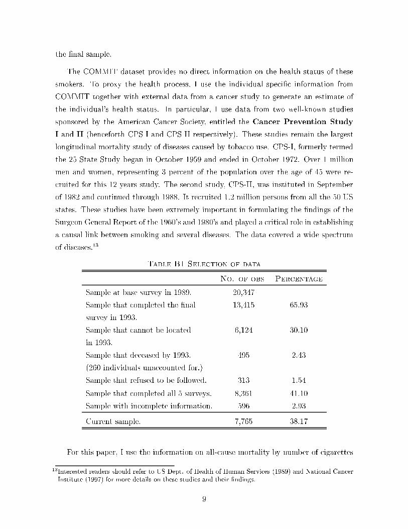
the �nal sample.
The COMMIT dataset provides no direct information on the health status of these
smokers. To proxy the health process, I use the individual speci�c information from
COMMIT together with external data from a cancer study to generate an estimate of
the individual's health status. In particular, I use data from two well-known studies
sponsored by the American Cancer Society, entitled the Cancer Prevention Study
I and II (henceforth CPS-I and CPS-II respectively). These studies remain the largest
longitudinal mortality study of diseases caused by tobacco use. CPS-I, formerly termed
the 25 State Study began in October 1959 and ended in October 1972. Over 1 million
men and women, representing 3 percent of the population over the age of 45 were re-
cruited for this 12 years study. The second study, CPS-II, was instituted in September
of 1982 and continued through 1988. It recruited 1.2 million persons from all the 50 US
states. These studies have been extremely important in formulating the �ndings of the
Surgeon General Report of the 1960's and 1980's and played a critical role in establishing
a causal link between smoking and several diseases. The data covered a wide spectrum
of diseases.13
Table B1 Selection of data
No. of obs Percentage
Sample at base survey in 1989. 20,347
Sample that completed the �nal 13,415 65.93
survey in 1993.
Sample that cannot be located 6,124 30.10
in 1993.
Sample that deceased by 1993. 495 2.43
(260 individuals unaccounted for.)
Sample that refused to be followed. 313 1.54
Sample that completed all 5 surveys. 8,361 41.10
Sample with incomplete information. 596 2.93
Current sample. 7,765 38.17
For this paper, I use the information on all-cause mortality by number of cigarettes
13Interested readers should refer to US Dept. of Health of Human Services (1989) and National CancerInstitute (1997) for more details on these studies and their �ndings.
9

smoked, attained age and duration of smoking to parameterize the relationship between
the mortality risk ratio for current smokers and these individual speci�c characteris-
tics.14 A polynomial log model of smokers characteristics is �tted over these data. Table
3.2 compares the risk ratio estimates with that reported in National Cancer Institute
(1997) for the study CPS I for two consumption levels. The log model gives a reasonable
overall �t to the data. This model is used together with the mortality rates from the
1991 Life Tables (for a non-smoker) to estimate the mortality rates for the COMMIT
data.
Insert Table 3.2 here
3.1 Preliminary Analysis of the Data
This section provides some descriptive statistics. An observation at year t is the
average number of cigarettes smoked per day by the enrolled individual during the time
of the annual interview.15 I de�ne quit to mean that the smoker reported zero consump-
tion on the day of the interview.16 Table B2 shows the quit dynamics of the data. All
individuals upon enrolment are smokers. The mean for the sample at the start of the
study is about 23 cigarettes smoked per day.
Table B2 shows that 18 percent of the sample reported quitting in the �rst period,
1990, and this percentage gradually increases to 31 percent of the sample in the �nal
period, 1993 (as shown by �gures in the �rst column). Around a third of those that
quit in 1990 relapse in the second period, 1991. In the sample of continuing smokers in
1990, 10 percent of these individuals will report zero consumption in 1991 and so on.
This table help illustrate the quitting dynamics in the data. A dynamic model of smok-
ing should be able to generate these dynamics of quits and relapses. Out of the entire
sample, 58 percent never quit over the period of the study while 11 percent successfully
quit for all four periods as shown in the last row.
14The mortality risk ratio is the ratio of the death rate of a smoker (usually expressed in number ofdeaths per 100,000 persons), over that of a non-smoker.
15This average was constructed using the reported cigarettes smoked on a weekday and that smokedduring the weekend.
16This de�nition is obviously very loose and potentially problematic since the smoker could have justattempted to quit and resumed smoking the day after the interview. The NCI used a stronger require-ment in that the individual has to stop smoking for at least six months to attain the quit status. Assuch, the dataset does provide information on whether the smoker was smoking six months prior tothe date of the interview but not the actual amount the smoker was consuming. I have decided toignore this censored information for now as it complicates much of the econometrics in the modellingsection. I hope to include this additional information in future revisions of the paper.
10

Table B2 : Quitting Dynamics on full sample.
Year Total sample
% that quit n=7765
1990 18.49% 81.51%
18.49% (1436)Q (6329)S
1991 13.19% 5.31% 9.45% 72.05%
22.64% (1024)Q (412)S (734)Q (5595)S
1992 11.90% 1.29% 1.47% 3.84% 6.04% 3.41% 7.17% 64.88%
26.58% (924)Q (100)S (114)Q (298)S (469)Q (265)S (557)Q (5038)S
1993 11.06% 57.64%
31.06% (859)Q (4476)S
S and Q denotes the subsamples that smoke and quit respectively.
Most of the numbers for 1993 have been omitted for space considerations.
Table B3 shows some statistics comparing the various quit samples. The sample that
stopped smoking over the entire length of the study are on average older, and of higher
average income compared to the sample that never quits, or that which quit for only
a single period. This sample also smoke a smaller amount on average upon enrolment
in the study and started smoking at a later age. Further analysis of these data also
show that the subsample that successfully quit the entire period of the study are on
average more educated and hold more 'white collar' jobs. This feature of the data also
arises in reduced form regressions with these demographic characteristics. Of the sample
that never quit, I �nd that these smokers tend to smoke a relatively constant amount
throughout the study period. Smokers usually remain in the cigarette bracket that they
started with upon enrolment in the study.
One of the features of the dataset that is not ideal is the absence of any informa-
tion about the purchasing behavior of the smoker or the price that they pay for their
cigarettes. Cigarettes are di�erentiated mainly by unobserved taste and some observ-
able attributes like length, size, nicotine and tar content, advertising, etc. Firms set a
national wholesale price, on which the state and federal government levy an excise tax
followed by the retailer's and wholesaler's markup. The classic argument in a di�eren-
tiated products framework for instrumenting for price even when using individual level
11

data is the unobserved product quality is most likely correlated with price.
Table B3 : Descriptive Statistics on various sub-samples
Sub-sample that
never quit for quits for Full
Variables quits 4 periods 1 period sample
(n = 4467) (n = 858) (n = 1183) (n = 7752)
Mean Age 41.0 42.5 40.8 41.2
in 1989. (10.2) (11.2) (10.4) (10.5)
Mean cig. 25.1 19.4 22.4 23.2
smoked in 1989. (12.1) (12.7) (12.3) (12.5)
Mean 17.8 18.6 18.1 18.0
starting age (4.1) (4.4) (4.3) (4.2)
Median daily 93.92 101.50 100.35 96.80
Incomey 1990 US$ (57.1) (58.4) (58.1) (57.6)
Std. error in parenthesis. y Median income is calculated for each respective income groups,
measured in 1990 US$.
Intuitively, we expect price to be high when the unobserved component of demand
is high hence generating this correlation. The natural remedy would be to instrument
for price using cost shifters. Moreover in this scenario where price information is un-
observed, there is an additional problem of measurement error. In the regressions that
follow, I have chosen to instrument for price to remedy these econometric problems.
The price series used is the weighted average retail price for the state, measured in 1990
US$.17 This is instrumented on average hourly earnings in the state, average price for
Burley and Flue-cured tobacco18, state and federal taxes measured in 1990 US$, and
state and time dummies.
Insert Table 3.3 here
17The price data is the nominal weighted average price for a pack of cigarettes for the state takenfrom Table 13a Tobacco Institute (1994), The Tax Burden on Tobacco, compiled by the now defunctTobacco Institute. This prices include state and federal levied excise tax but does not include municipalor county excise tax nor sales tax. The data for 1990 to 1994 takes into account the generic brandcategory of cigarettes. These data is subsequently de ated by the CPI.
18This is taken from the USDA Tobacco website.
12

Table 3.3 shows two stage least squares (2SLS henceforth) cross-sectional regressions
for three periods of the sample. The dependendent variable ln(1 + Ct), is regressed
on instrumented log prices, ^ln(Pt), and individual demographic characteristics. In the
�rst period of the study 1989, we �nd that the coeÆcient on price is not signi�cantly
di�erent from zero. The estimates suggest that smokers in states with higher prices are
not on average smoking less than smokers in states with lower cigarette prices. In the
regressions for 1991 and 1993, we �nd that the coeÆcient on price becomes signi�cant.
Quitting behavior is crucial in identifying the price coeÆcients. These estimates indicate
that quitting rate is higher in states with higher average prices con�rming its role as
an e�ective regulatory instrument. The price elasticities of 0:25 to 0:37 also fall in the
range obtained by previous empirical work using similar forms of analysis.
Insert Table 3.4 here
The estimates on the remaining variables suggest the following empirical facts about
the various covariates: smokers who are older, started smoking later, more educated and
of higher income group are on average more likely to quit; female smokers on average
smoke less than male smokers; smokers who hold 'blue collar' jobs are less likely to quit.
This empirical features of the data also arise in Table 3.4 which shows cross-sectional
probit regressions for the period 1990 and 1993. The indicator for an intervention com-
munity from both these sets of regressions do not seem to be a major explanatory variable
for quitting behavior.
This preliminary analysis of the data helps highlight some facts about smoking ces-
sation. Statistically signi�cant predictors of quitting behavior include higher income,
higher education, older age, later starting age and being male. This is in line with the
�ndings in other papers.19
4 The Model
This project began with a much simpler habit formation model, with prices and the
addiction stock as the only state variables. This model could not capture much of the
dynamics of the data. In particular, it underpredicts the proportion of quits and pro-
vides unrealistic estimates of the price elasticity. A discussion of this preliminary model
is included in Section 7.3 of the Appendix. In this section, I will provide a general
19See Wasserman, Manning, Newhouse, and Winkler (1991) and Hu, Ren, Keeler, and Bartlett (1995)
13

overview of the main model (that incorporates the health process as a state variable),
and the estimation approach. This will be followed by an outline of the assumptions in
Section 4.2 and the estimation procedure in Section 4.4.
4.1 Overview of the model and the estimation procedure
The smoker is assumed to have a set of well de�ned preferences (represented by
a static utility function), which is time separable and does not change over time. The
individual maximizes the sum of discounted expected utility, in a manner consistent
with his preferences and beliefs about the states that a�ects well-being. Addiction is
modeled as a unobserved `stock' that accumulates stochastically. Current consumption
provides instantaneous utility to the smoker and also adds linearly to this stock, which
depreciates at a constant rate. This stock variable a�ects the marginal utility of future
consumption, capturing the reinforcement feature of addictive consumption. The ac-
cumulation process is stochastic in that a random component also adds linearly to this
unobserved addiction stock. This disturbance summarizes other unobserved factors that
in uence the smokers decision each period.
Health is approximated by a discrete state variable.20 For now, the individual is
assumed to be in one of three possible states, either high, low or an absorbing terminal
state of health. This discrete process evolves according to a �rst order Markov process.
The realization of next period's health state depends on its current realization, the vec-
tor of current states, the individual's characteristics, and the individual's action this
period.
The characteristics that in uence how health evolves, like age, gender, and smok-
ing history (as represented by the duration of smoking and the amount the individual
smokes on average), is summarized by two statistics, the individual's mortality rate and
mortality risk ratio. I assume that a smoker is endowed with these two statistics at the
beginning of the program. These statistics are computed using data from CPS I and the
1991 Life Tables, and are a source of individual heterogeneity. The mortality risk ratio
measures the excess mortality incurred by the smoker from his history of smoking.21
20In reality, health status obviously does not take discrete values and is in uenced by many factors thatare dynamic. However, to model this complex process in a computationally tractable way, I resort tothis simple �rst approximation.
21This is measured by the ratio of the death rate of a smoker with the de�ned characteristics and smoking
14

The probability that the individual enters the terminal state next period is determined
by the mortality rate. The probablity that the smoker draws a low health state next
period depends on these two statistics and his decision in the current period.
Smoking increases the probability that a worse health state occurs next period and
indirectly increases the likelihood of entering the terminal state sooner. This cost where
continual smoking brings the smoker closer to an undesired state, is factored into the
smoker's decision each period. The notion of a lower state of health is purely academic
and need not be associated with the occurrence of any serious smoking associated ill-
nesses, rather it is meant to capture either a lower state of well-being, or a realization
that the smoker is closer to an absorbing terminal state as a results of his addiction,
hence creating an incentive to quit. This incentive however is weakened by the fact that
the individual gets utility from smoking and from accumulating the addictive stock.
This model also allows the cost incured at the low health state to vary according to
the individual's demographic characteristics. Quitting in this model can be a preventive
remedy that lowers the probability that a worse health state occurs, hence improving
the smoker's health prospects in the future. In the event that a worse health state ac-
tually occurs, quitting in this model can also be curative remedy, where it increases the
probability that the smoker improve his or her health status in the future.
Estimation is based on the likelihood of a sample path of observed behavior condi-
tional on the initial values of the observed behavior and vector of states. To assign a
likelihood to any observed path, the model is �rst solved numerically at the observed
realization of prices, individual characteristics, and all possible realizations of the health
status. The solution procedure entails numerically computing the value function22 and
the policy rule as a function of the states. Certain functional form restrictions allow us
to compute the values of the unobserved states associated with observed behavior. A
likelihood can then be assigned to the observed consumption path.23 This is followed by
standard maximum likelihood procedures.
history, over that of a non-smoker with similar characteristics. The mortality rate for that individual issimply the product of this risk ratio and the mortality rate of non-smoker with the same characteristics.
22Which represents the lifetime total present discounted expected utility.23An detailed discussion of the intuition behind the estimation methodology is provided in Pakes (1996)for the case of modelling the investment decision of a �rm where the unobserved state is the �rm'sproductivity. The approach is also similar to that used by Timmins (2000) where the author modelsthe pricing decision of the municipal owned water utilities; the unobserved state in that problem is thenet marginal revenues in the water utilities' pro�t function.
15

4.2 Assumptions and Definitions
A representative smoker at each period t decides whether to quit or continue smok-
ing ct cigarettes so as to maximise the sum of discounted expected utilities. The decision
space is bounded and is denoted by D = [0; �C]. The agent is in�nitely lived with the
possibility of entering an absorbing terminal state. The individual is concerned about a
vector of four state variables, fHt; It�1; It; ; atg. I will �rst explain these state variables.
The agent's smoking status in the previous period is denoted by It 2 f0; 1g.
It takes a value of 1 if he quits in the previous period and 0 otherwise. This indicator
summarizes information about the agent's smoking history and directly a�ects the evo-
lution of the health process, Ht.24
The agent's instantaneous marginal utility from consumption depends on a stock
of addictive substance, at, which is known to the smoker but unobserved by the
economic analyst. Like ct, this state variable is also bounded, at 2 [0; �A]. It decays
stochastically over time and the smoker's current consumption adds linearly to it as
shown in Equation 4.1.
at+1 =
((1 + Æ0)at + Æ1ct + �t+1; : �t+1 � N(0; �2� ) if 0 � at+1 � �A
�A or 0 : otherwise(4.1)
The rate of decay is denoted by Æ0, where Æ0 2 (�1; 0). at is a measure of the smoking
history of the individual and needs to be recovered so as to assign a conditional likelihood
to any observed consumption, ct. � denotes the set of parameters de�ning the stochastic
process of at, that is,
� = fÆ0; Æ1; ��g:
The state variable, Ht, represents the health status of the agent at period t. It
takes three discrete values, Ht 2 fhH; hL; hTg and evolves according to a Markov decision
process. The state, hH, denotes a good state of health, hL denotes a bad state, which
can be thought of as a negative health event, and hT, the terminal state. The agent, for
now, is assumed to have a constant discount factor � 2 (0; 1), which does not depend
on either state or choice variables.25
24For now, both It and It�1 are assumed to have no direct e�ect on the smoker's intantaneous utility.25The framework is suÆciently exible to allow for state dependent discount factor as well as hyperbolicdiscounting. This is a feature I will consider when performing policy experiments.
16

The state vector for this model is denoted by st = fHt; It�1; It; ; atg, it lives in a
state space S= fhH; hL; hTg � f0; 1g � f0; 1g � [0; �A]:
Each smoker i is endowed with a characteristics vector denoted xi = fmi; P; Yi; ri;
�i; gi; zig
�i: Mortality rate if individual i were a non-smoker.26
ri: Relative risk ratio re ecting smoker's i smoking history and characteristics.27
mi: Mortality rate for smoker i, where mi = ri � �i.
P : Price.
Yi: Real Income (in 1990 US $) for smoker i.
gi: Average age of smoker i.
zi: other individual speci�c characteristics.
These variables are assumed to be constant over time with the exception of price,
P . The smoker takes price as given and does not expect it to change. Even though
the agents are assumed to be naive about prices, the estimation will involve solving the
model at each observed price. This simplication does not in any way compromise the
analytic power of the model. I estimated an earlier model that considers price as a state
and found that this does not contribute much to the prediction of smoking and quitting
behavior28.
The factors that in uence the health process change over time and depend on the
smoker's decision each period. Introducing these various individual characteristics as
actual states variables that in uence the health process would be computatationally
very expensive. Given the short time period of the data and the fact that all individuals
are `seasoned' smokers, I will assume that the smokers are endowed with a risk ratio,
ri, and a mortality rate, mi, that does not change over the periods of the sample. In
e�ect, the risk ratio and mortality rate become suÆcient statistics for the individuals'
characteristics and smoking history. The health process depends on the endowed risk
ratio, mortality rate and the smokers decision to smoke or quit. The mortality rate of
the smoker, mi, is given by the product of this relative risk ratio, (ri,) and mortality
rate of a non-smoker with the same age and individual characteristics pro�le (�i).29
26This is calculated from 1991 Life Tables.27This is estimated using CPS I and II.28I have included description of this earlier model in Section 7.3 of the Appendix.29Given the assumption that the factors in uencing the mortality rates are constant over time, the
17

The health state variable evolves according to a �rst order Markov process with a
probability transition matrix, H(�), given by Equation 4.2 below.
H(mi; ct; It; It�1; zi; �) =
2666664
(1�mi)exp(
it)
1+exp( it)
(1�mi)1
1+exp( it)
mi
(1� �mi)1
1+exp(!it)(1� �mi)
exp(!it)1+exp(!it)
�mi
0 0 1
3777775 (4.2)
The transition probability depends on ct and all elements of the state vector except
for the actual stock of addiction, at. Given that both at and Ht are both unobserved,
this assumption ensures that the joint distribution of these states take a simple form.
This will be futher explained in Section 4.4. I will use the conventional Markov chain
notation, PHL, to denote the probability of the event Ht+1 = hL, given that fHt =
hH; ri; mi; Ifct > 0g; It; It�1g, that is,
PHL = PfHt+1 = hL j Ht = hH; ri; mi; Ifct > 0g; It; It�1; �g
=1�mi
1 + exp( it)
The terms it and !it in the logit probabilities are linear functions of the variables
fri; mi; Ifct > 0g; It; It�1g. The term it in the logit probabilities takes the form,
it = 0 + 1ri + 2mi + 3Ifct > 0g+ 4It+ 5It�1+ 6It�1It: (4.3)
Intuitively, the probability of a negative health event, hL, is increasing if the individual
continues to smoke. It is also increasing in the duration of smoking and the age of the
smoker. This would be re ected by a large value of mi, and ri. Introducing both these
terms allows us to di�erentiate between two individuals of the same mortality rate, mi,
but di�erent age, and smoking history. These di�erences are re ected by di�erent risk
ratios, ri. The terms ri, mi, and Ifct > 0g, capture the morbidity of smoking addiction.
The likehood of a negative health incident is decreasing in It and It, capturing the health
individually endowed mortality rates, are calculated at the average age of the individuals in the study.
18

bene�t to quitting.30 The interaction term represented by the parameter 6 captures
the health gains associated with quitting for consecutive periods.
The term !it has a similar functional form,
!it = !0 + !1ri + !2mi + !3Ifct > 0g+ !4It+ !5It�1+ !6It�1It: (4.4)
!it captures the opposite e�ect to it. It is increasing in ri; mi, and Ifct > 0g and
decreasing in It�1 and It. The morbidity of smoking and the health bene�ts to cessation
is a multi-faceted and complex process that depends on many factors.31 Accounting for
these di�erent factors will be computationally infeasible and will put unrealistic demands
on what the data can provide. The above representation is chosen to an intuitive �rst
approximation of the health process that capture some of the main features of smoking
and quitting. This speci�cation can be made richer given more detailed data. The vector
� denotes the parameters of the health process Ht, where,
� = f�; 0; : : : ; 6; !0; : : : ; !6g
The agent's single period utility function is denoted by u(ct; st;xi;�) = ut. It
is additively separable and stable over time. The functional form for ut is chosen such
that it is well-de�ned and bounded over the state space S and decision space D . It takes
the following form,
u(ct; st;xi;�) =
8<:� (ct; st;xi;�) : ct � 0; Ht 2 fh
H; hLg
0 : 8 ct; Ht 2 fhTg:
The utility in the terminal state, Ht = hT, has been normalized to zero. For ct > 0
and Ht 2 fhH; hLg, the function � (:), takes the following form.
� (ct; st;xi;�)
= 0 ln(1 + ct) + 1at ln(ct) + 2Pct + 3 ln(Y ) + 04gi + 5 (4.5)
+ IfHt = hLg(�0 ln(1 + ct) + �1at ln(1 + ct) + �3 ln(Yi) + � 04gi + �5):
30As supported by a large body of medical evidence, examples include US Dept. of Health of HumanServices (1989) and US Dept. of Health of Human Services (1990)
31US Dept. of Health of Human Services (1990) provides a discussion of the bene�ts of smoking cessation.
19
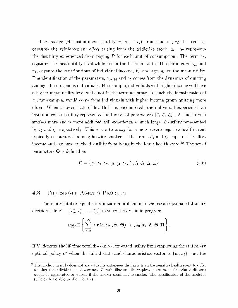
The smoker gets instantaneous utility, 0 ln(1 + ct), from smoking ct; the term 1,
captures the reinforcement e�ect arising from the addictive stock, at. 2 represents
the disutility experienced from paying P for each unit of consumption. The term 5,
captures the mean utility level while not in the terminal state. The parameters 3, and
4, capture the contributions of individual income, Yi, and age, gi, to the mean utility.
The identi�cation of the parameters, 3; 4 and 5 comes from the dynamics of quitting
amongst heterogenous individuals. For example, individuals with higher income will have
a higher mean utility level while not in the terminal state. As such the identi�cation of
3, for example, would come from individuals with higher income group quitting more
often. When a lower state of health hL is encountered, the individual experiences an
instantaneous disutility represented by the set of parameters f�0; �1; �5g. A smoker who
smokes more and is more addicted will experience a much larger disutility represented
by �0 and �1 respectively. This serves to proxy for a more severe negative health event
typically encountered among heavier smokers. The terms �3 and �4 capture the e�ect
income and age have on the disutility from being in the lower health state.32 The set of
parameters � is de�ned as
� = f 0; 1; 2; 3; 4; 5; �0; �1; �3; �4; �5g: (4.6)
4.3 The Single Agents Problem
The representative agent's optimization problem is to choose an optimal stationary
decision rule c� = fc�i0; c�i1; : : : c
�i1g to solve the dynamic program,
maxc�
E
(1Xt=0
�tu(cit; st;xi;�) j c0; s0;xi;�;�;�
):
IfVt denotes the lifetime total discounted expected utility from employing the stationary
optimal policy c� when the initial state and characteristics vector is fst;xig, and the
32The model currently does not allow the instantaneous disutility from the negative health event to di�erwhether the individual smokes or not. Certain illnesses like emphysema or bronchial related diseaseswould be aggravated or worsen if the smoker continues to smoke. The speci�cation of the model issuÆciently exible to allow for this.
20
parameters set at the values f�, �, �g, that is, Vt = Vc�(st j xi;�;�;�), the
Bellman's operator for this single agent's problem is then given by,
Vt = maxc�fu(ct; st;xi;�) + � E (Vt+1 j ct; st;xi;�;�;�))g: (4.7)
The assumptions made in Section 4.2 satisfy the suÆcient conditions for the Contraction
Mapping Theorem to apply.33 This ensures that there exists a unique �xed point to the
Bellman's operator and that a non-empty stationary policy rule, � : S 7! D , exists and
is of the form shown in Equation 4.8. Using the properties of the contraction mapping,
the �xed point Vt can be solved by successive approximation methods and the policy
rule can be solved numerically by policy improvement techniques.
c�t = argmaxc�t
fu(ct; st;xi;�) + � E (Vt+1 j st;xi;�;�;�)g
= �(st j xi;�;�;�) = �t, where c�t 2 D ; (4.8)
Given the de�nition of the Markovian state variables, the expectation in the Bell-
man's oparator can be written in the following separable form,
E (V(st+1 j ct; st;xi;�;�;�))
=
ZH
Za
V(st+1) � }�(at+1 j Ht+1; ct; st;�;�) � }H(Ht+1 j ct; st;�) dat+1 dHt+1
=X
Ht+12fhH;hLg
}H(Ht+1 j ct; st;�) �
Za
V(st+1) � }�(at+1 j Ht+1; ct; st;�;�) dat+1 :
4.4 Estimation
I now outline the estimation strategy that I adopt in this paper. I have borrowed
heavily from theories and numerical methods employed in solving and estimating mixed
discrete and continuous Markov Decision Process. These areas have been heavily re-
searched and interested readers should refer to Pakes (1996), Rust (1994), Timmins
(2000) for more in depth discussion.
A Nested Fixed Point Maximum Likelihood Estimation method is used to estimate
the parameters of this model. This algorithm comprise of two loops. An outer loop
33Interested readers should refer to Ross (1970), Lucas and Stokey (1989), and Rust (1996)
21

solves for the parameter that maximise the likelihood of the sample of data. An inner
loop solves for the �xed point of the value function, the policy rule, and calculates the
implied conditional likelihood corresponding to a set of parameter values. A modi�ed
policy iteration method is adopted to solve for the �xed point to the Bellman Equa-
tion 4.7 conditional on f�̂; �̂; �̂;xig. This is used together with the Brent's numerical
method that solves for the mixed discrete and continuous optimal control. This is car-
ried out on a discretized state space.
These dynamic programming numerical procedures solve for the policy rule �(:),
as a function of the state vector, st. The maximum likelihood estimation approach
requires that a likelihood be assigned to the tuple fct; stg conditional on fct�1; st�1;
xi;�;�;�g. This means that we need to recover the unobserved states, fat;Htg, from
the solved policy rule �t. The static one period utility is de�ned to be non-decreasing in
the unobserved state at, holding everything else constant. This condition would ensure
that the the policy function is also non-decreasing in at.34 This restriction on the utility
function provides an invertibility condition that allows the recovery of the unobserved
state, at = ��1(ct = c�; Ht; It�1; It j xi;�;�;�). This condition states that every vector
fc�;Ht; It�1; Itg is only associated with a single value of the unobserved state at.
This approach precludes the introduction of the tolerance e�ect in the manner consid-
ered in existing theoretical model of rational addiction like Becker and Murphy (1988).
Allowing the policy rule to be non-monotonic in at creates a non-uniqueness complication
that would make the estimation problem not tractable. I believe that this restriction is
not an unreasonable approximation of the cigarette addiction process. However, there
are many examples of addiction like that of alcohol and cocaine addiction where this
assumption is unrealistic. In these forms of addiction, there are signi�cant negative
health e�ects associated with accumulating the addiction stock. In future extension
of this paper, I intend to relax this assumption by resorting to alternative estimation
methods. A minimum distance estimation approach in which the metric is the euclidean
norm between the implied and observed moment conditions is a possible alternative.
The potential complication in that approach is the choice of moment conditions. This
will be a topic of further extensions of this paper.35
34A formal statement and proof of this result is given in Lemma 3 of Pakes (1996).35There is also the added issue that the state Ht is also unobserved and the de�ned invertibility conditionrequires this state to be an element of the conditioning vector fc�;Ht; It�1; Itg. I will consider two
22

Figure 4.1: Illustration of a stylised policy function.
-
6
at
ct
~aL~aH??
aLitaHit
cit
0
�(at; ct j Ht = hL;xi; �̂; �̂; �̂)�(at; ct j Ht = hH;xi; �̂; �̂; �̂)
Figure 4.1 illustrates a stylized policy function, conditional on a set of parameter val-
ues, characteristics vector and states fIt; It�1;Htg. The monotonicity property allows
the unobserved ai, corresponding to the observed ci > 0, to be solved through simple
interpolation. The diagram shows that the amount of cigarettes smoked, ct, is increasing
with the level of addiction, at, holding the remaining states �xed. The amount consumed
conditional on an addiction stock at is lower when Ht = hL.
In a sample of T observations, the estimation algorithm de�nes a likelihood for the
sample path, fci2; si2; : : : ; ciT ; siTg, conditional on the observation vector, fci1; si1g, at
period t = 1. Given the de�nition of the stochastic process Ht in Equation 4.2, where
the realization of Ht+1 depends only on fmi; ct; It; It�1; zi; �g, the joint distribution of
alternative ways of dealing with this initial condition problem. The �rst would be to naively assumethat Ht = hH at the beginning of the sample. The second would be to calculate the stationarydistribution associated with the irreducible portion of the Markov chain and assign individuals to thishealth state according to this distribution.
23

the two unobserved states have a simple separable form,36
P(ci2; si2 j ci1; si1;xi;�;�;�)
=X
Hi22fhH;hLg
Ifci2 = �2; Hi2g � }�(ai2 = ��12 j Hi2; ci1; si1;�;�) � }H(Hi2 j ci1; si1;�)
The data tracks the behavior of smokers over a period of 5 years, each smoker i starts
in period t = 1 smoking some positive amount, ci1 > 0. I will suppress the index for
individual smokers for now. Consider the case where an individual smokes a positive
amount throughout the entire sample period, the likelihood of observing fc2; s2g will be,
`(c2; s2 j c1; s1; �̂; �̂; �̂)
=X
H22fhH;hLg
Ifc2 = �2; H2g � }H(H2 j c1; s1; �̂)
� f�(��12 � (1 + Æ̂0)�
�11 � Æ̂1c1 j H2; c1; s1; �̂; �̂)
where f�(: : :) denotes the normal density. The corresponding likelihood for the entire
consumption path for periods t = 2; : : : ; T of a smoker who never quits would be,
`(c2; : : : ; cT ; s2; : : : sT j c1; s1; �̂; �̂; �̂)
=TYt=2
� XHt2fhH;hLg
Ifct = �t; Htg � }H(Ht j ct�1; : : : ; c1; st�1; : : : ; s1; �̂)
� f�(��1t � (1 + Æ̂0)�
�1t�1 � Æ1ct�1 j Ht; ct�1; : : : ; c1; st�1; : : : ; st; �̂; �̂)
�
The dynamics in this smoking behavior(holding P �xed) are driven by the stochastic
process determining Ht and at. In Figure 4.1, these threshold levels of addiction are
denoted by ~aH when the individual is in the good state of health and ~aL when he gets
a negative health shock. If at falls below this threshold, the smoker stops smoking for
36For example, the probability of observing fci2; si2g conditional on fci1; si1g, where Hi1 = hH, will be
P(ci2; si2 j ci1; si1;xi;�;�;�)
= Ifci2 = �2; Hi2 = hHg � }�(ai2 = ��12
j Hi2 = hH; ci1; st;�;�) �PHH
+ Ifci2 = �2; Hi2 = hLg � }�(ai2 = ��12
j Hi2 = hL; ci1; st;�;�) �PHL:
24

that period t. As such, quitting, even after conditioning on the unobserved Ht, creates
an indeterminacy of the stock of addiction for that period. The likelihood for that
individual requires that the indeterminate at be integrated out. To illustrate, consider
the case where a smoker is smoking in period one, quits in period t = 2, relapses in period
three and continue smoking the remaining periods. The likelihood of this consumption
path would be,
`(c2; : : : ; cT ; s2; : : : ; sT j c1; s1; �̂; �̂; �̂)
=TYt=4
� XHt2fhH;hLg
Ifct = �t; Htg � }H(Ht j ct�1; : : : ; c1; st�1; : : : ; s1; �̂)
� f�(��1t � (1 + Æ̂0)�
�1t�1 � Æ1ct�1 j Ht; ct�1; : : : ; c1; st�1; : : : ; st; �̂; �̂)
�
�XH3
XH2
Ifc3 = �3; H3g � Ifc2 = �2; H2g � }H(H3 j c2; c1; s2; s1; �̂) � }H(H2 j c1; s1; �̂)
�
Z ~�H2
�1
f�(��13 � (1 + Æ̂0)�
�12 j c2 = 0;��12 � ~aH2 ; s2; c1; s1; �̂; �̂)
� f�(��12 � (1 + Æ̂0)�
�11 � Æ̂1c1 j c1; s1; �̂; �̂))d�
�12 : (4.9)
where ~�H2 2n~aH � (1 + Æ̂0)a1 � Æ̂1c1; ~a
L � (1 + Æ̂0)a1 � Æ̂1c1
oand ~aH2 2
n~aH; ~aL
o
Hence each quit observation would generate an integral in the likelihood calculation.
There is a total of sixteen possible likelihood formulations (depending on the quitting
patterns observed) and another sixteen possible permutations of the health state for
the sample of �ve periods used in this paper. I have chosen to leave these various
likelihood formulation out of the paper, they are available on request from the author.
The likelihood for the entire sample would simply be the product of all the individual
likelihood functions, that is,
Ln =nY
i=1
`(ci2; : : : ; ciT ; si2; : : : ; siT j ci1; si1;�;�;�) (4.10)
25

5 Monte Carlo Simulations
This section discusses the Monte Carlo simulation of the structural model described in
Section 4.2. It illustrates the kind of dynamics that the model can generate and provides
a prima facie test of whether the model can explain data. Table 5.1 shows the parameters
values used in the simulation. The �'s have been set to zero. The values for the terms, 0,
1 and 2, are set close to those obtained from the estimation of a preliminary model.37
The remaining parameters are set by trial and error. The probability transition matrix
of Ht at this parameter values for two combinations of the state vector are given below,
P(Ht+1 j Ht; It = 0; It�1 = 0; ct > 0;�) =
2664
0:674 0:321 0:005
4:2� 105 0:800 0:200
0:000 0:00 1:000
3775
P(Ht+1 j Ht; It = 0; It�1 = 0; ct = 0;�) =
26640:676 0:319 0:005
0:420 0:380 0:200
0:000 0:000 1:000
3775
Insert Table 5.1 here.
The parameters of the health process are chosen such that a smoker in the good
state (Ht = hH), has approximately 30 percent chance of a negative health event next
period.38 In the event of a negative health shock, quitting is essentially necessary for the
smoker to have a reasonable chance of returning to the high health state.39 With the
values of �'s set to zero, a negative health event does not bring instantaneous disutility
but it does bring the individual closer to the absorbing terminal state.
The characteristic vector for the representative agent is set to the mean value for
the Massachusetts. The mean age is 41, the average daily consumption is a pack (20
cigarettes), and the average duration of smoking is 18 years. The relative risk ratio, ri,
for a smoker with these mean characteristics is around 2, and the corresponding mortality
37A discussion of this model is included in Section 7.3 of the Appendix. This preliminary model isestimated using a sub-sample from the state of Massachusetts.
38For example, the �rst matrix shows that an individual who continues to smoke has a 32.1 percentchance of drawing a bad state next period. Someone who quits has a slightly lower chance, 31.9percent, of incurring a bad state next period.
39So from the �rst transition matrix, someone in a bad state of health who continues to smoke has anarrow chance of covering back to the good state, (0.004 percent,) and 20 percent of entering theterminal state next period. If the individual quits, he has a 42 percent of recovering back to the goodstate.
26

rate, mi, is around 0.005. The model is �rst solved at the parameter values and observed
cigarette prices for the period 1989 to 1993. The model is then simulated starting from
the observed empirical distribution of consumed cigarettes for the year 1989. Random
numbers for �t and Ht are drawn according to the prede�ned stochastic processes. The
time path of the smokers' decisions are then computed according to the solved policy rule.
Figure 5.1 : Value Function and Policy Rule
for the simulated sample.
Figure 5.1 shows the value function and policy rule at some combination of the
state vector for the year 1991. Figure (a) illustrates the solved value function as a
function of the addiction stock, at, at the two health states, and the quitting history
fIt = 1; It�1 = 1g and fIt = 0; It�1 = 0g. As expected, the value function for an
individual in the good health state who has not smoked in the previous two periods,
V(at j hH; It = 1; It�1 = 1), is greater than if he smoked the previous two periods,
V(at j hH; It = 0; It�1 = 0). Quitting lowers the chance that a negative health event
occurs next period and hence increases the sum of discounted expected utility.40 The
40By the same logic, the value function at the low state of health, hL, is also lower than the correspondingvalue functions at hH, holding everything else equal.
27

kink in the value functions at hL corresponds to the kink in the policy function at hL
shown in Figure (b). The transition probabilities are de�ned to depend only on the cur-
rent decision of whether to smoke or quit, and not on the actual level of consumption.
As such, when the stock of addiction gets to a critical level where it pays to resume
smoking, the smoker will consume up to a level that conpensates him for the loss in
lifetime utility as a result of the increased probability from entering the terminal state.
This generates the kink in the policy function.
By construction, the policy rules are weakly increasing in the addiction stock. In-
terestingly, �(at j hH; It = 0; It�1 = 0), is lower than �(at j h
H; It = 1; It�1 = 1). That
is, conditional on a level of addiction stock, smokers at the high state of health and
who have not smoked in the previous two periods, smoke more than a smoker with the
same level of addiction but who has smoked the last 2 periods. A negative health event
enlarges the range of the addiction stock for which the smoker chooses not to smoke.
At these levels of the addiction stock, the increase in lifetime utility from smoking and
further accumulating the addiction stock is not o�set by the utility decrease from being
closer to the terminal state.
Table A1 : Statistics of obs. and sim. sample for state of MA. (n = 654)
obs. P % quits sub-sample of smokers, ct > 0
years in cents sim. obs. mean(s) stdev(s) mean(o) stdev(o)
1989 8.03 - 0.00 - - 24.05 12.46
1990 8.16 19.11 21.16 22.56 11.77 22.77 13.45
1991 8.44 29.51 26.79 18.83 10.64 22.46 11.27
1992 8.41 33.64 31.96 15.26 9.85 21.88 10.99
1993 8.62 37.77 35.16 12.02 7.94 21.49 10.84
Table A1, compares some general statistics of the simulated and observed sample.
The second column shows the observed price, P , and the third and fourth column show
the simulated and observed percentage of quits. The model generates quit percentages
that are in the range observed in the data. The current parameterization seems to over
predict the number of quits in 1991, and this appears to have a carry-over e�ect for the
subsequent years. This most likely results from demand being too sensitive to price41.
41Coupled with the likely inaccurate parameterization of the health process.
28

There is a large increase in price in 1991 relative to the previous years and the current
parameterization over-predicts the number of quits in that period. The remaining four
columns show statistics for the sample of smokers in each period. The distribution of the
simulated sample of smokers appears to have means and variances that are well below
what is observed in data. The mean consumption level also seems to be decreasing over
time. This is a feature of the model that estimation will likely improve upon.
Table A2: Simulated Quitting Dynamics for sample from MA
(observed percentage in parenthesis)
Year Total sample
% that quit n=654
1990
19.11 19.11 80.89
(21.16) (21.16)Q (78.84)S
1991
29.51 9.33 9.79 20.18 60.70
(26.79) (15.83)Q (5.33)S (10.96)Q (67.88)S
1992
33.64 4.13 5.20 2.29 7.50 9.32 10.86 17.89 42.81
(31.96) (14.76)Q (1.07)S (1.83)Q (3.5)S (7.31)Q (3.65)S (8.07)Q (59.82)S
1993
37.77 3.06 28.75
(35.16) (13.39)Q (52.66)S
S and Q denotes the subsamples that smoke and quit respectively.
Table A2 compares the proportions of the simulated and observed sample that quits
and relapses each period. The observed percentages are shown in parenthesis. The
�rst column shows the percentage of observed and simulated quits percentages for each
year of the sample (as previously shown in Table A1). The second row shows that 20
percent of the sample of smokers quit in the year 1990 of the study. The model predicts
that one-half of this subsample will continue not smoking in the following year (9.3
percent of the full sample). In contrast, in the observed data, around three-fourths of
the �rst period quitters remain quitters (15.8 percent of the original sample). Similarly,
the model predicts that one-fourth of the smokers in 1990 will quit in 1991, which
is around 20 percent of the full sample. According to the data, only one-eighth of the
29
sample of smokers in 1990 quits 1991. The current parameterization seems to overpredict
the proportion of quitters that will relapse and the proportion of continuing smokers
who will quit in the next period. This is something I expect actual estimation will
improve upon. Tables A1 and A2 highlight a very important feature of the model:
its ability to to generate both quitting and smoking dynamics as observed in data.
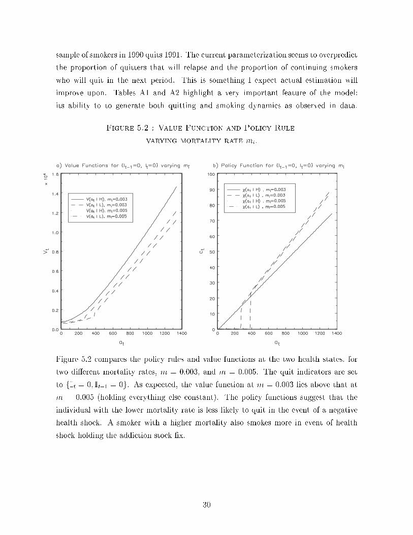
Figure 5.2 : Value Function and Policy Rule
varying mortality rate mi.
Figure 5.2 compares the policy rules and value functions at the two health states, for
two di�erent mortality rates, m = 0:003, and m = 0:005. The quit indicators are set
to fIt = 0; It�1 = 0g. As expected, the value function at m = 0:003 lies above that at
m = 0:005 (holding everything else constant). The policy functions suggest that the
individual with the lower mortality rate is less likely to quit in the event of a negative
health shock. A smoker with a higher mortality also smokes more in event of health
shock holding the addiction stock �x.
30

Figure 5.3 : Value Function and Policy Rule varying
mortality rate Æ1.
To illustrate the kinds of policy experiments possible with this model, consider a scenario
where we lower the amount of nicotine in cigarettes. This is equivalent to varying the
parameter Æ1 in the stochastic accumulation Equation 4.1. Table A3 shows statistics
from the Monte Carlo simulation of this experiment carried out for �ve periods and
Figure 5.3 shows the corresponding value functions and policy rules. Prices is held �xed
at 8:44 cents, which is the level observed in Massachusetts for 1991. The set of numbers
in the �rst three columns shows general statistics for the sample when Æ1 = 1:10. The
�rst column gives the percentage of the sample that quits each period. The second and
third columns give the mean and standard deviation of the subsample of smokers in each
period. The second set of columns shows statistics in the experiment where we lower
the amount that current consumption adds to the addiction stock by 10 percent which
is equivalent to setting Æ1 = 0:99.
31
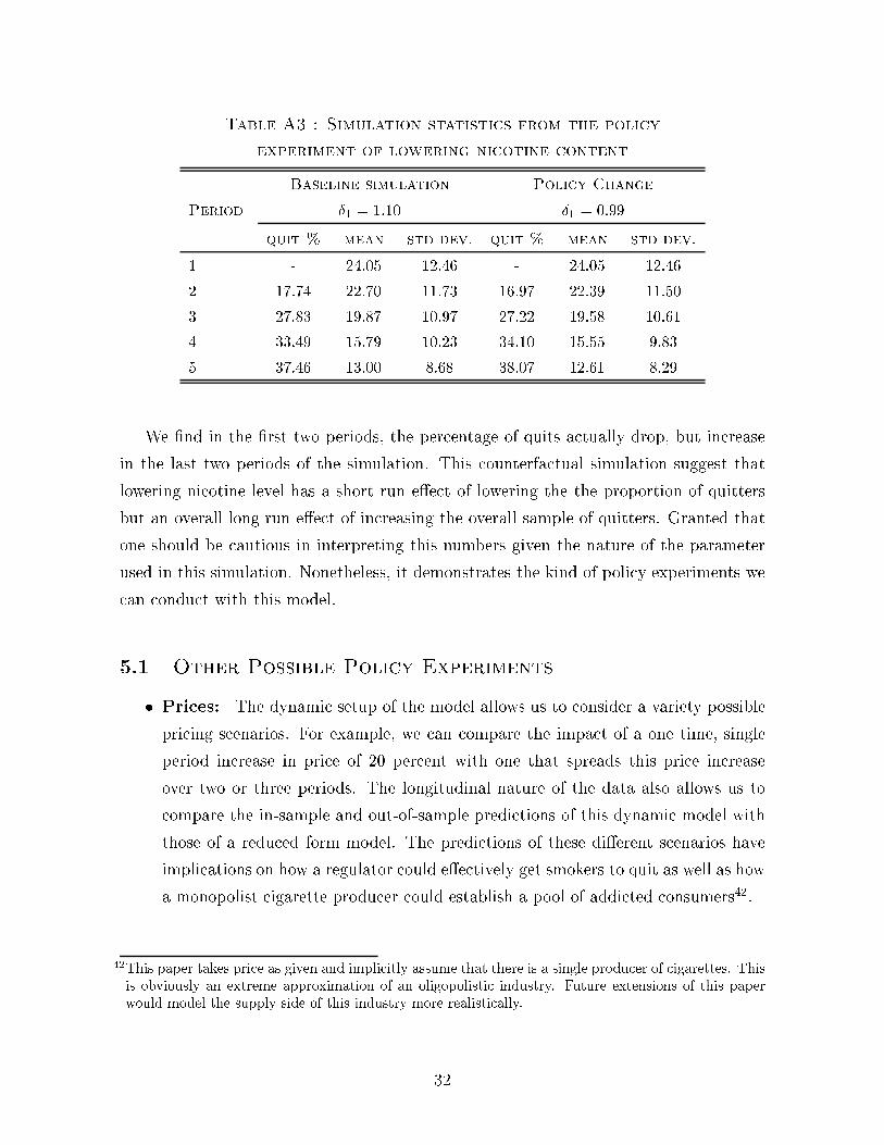
Table A3 : Simulation statistics from the policy
experiment of lowering nicotine content
Baseline simulation Policy Change
Period Æ1 = 1:10 Æ1 = 0:99
quit % mean std dev. quit % mean std dev.
1 - 24.05 12.46 - 24.05 12.46
2 17.74 22.70 11.73 16.97 22.39 11.50
3 27.83 19.87 10.97 27.22 19.58 10.61
4 33.49 15.79 10.23 34.10 15.55 9.83
5 37.46 13.00 8.68 38.07 12.61 8.29
We �nd in the �rst two periods, the percentage of quits actually drop, but increase
in the last two periods of the simulation. This counterfactual simulation suggest that
lowering nicotine level has a short run e�ect of lowering the the proportion of quitters
but an overall long run e�ect of increasing the overall sample of quitters. Granted that
one should be cautious in interpreting this numbers given the nature of the parameter
used in this simulation. Nonetheless, it demonstrates the kind of policy experiments we
can conduct with this model.
5.1 Other Possible Policy Experiments
� Prices: The dynamic setup of the model allows us to consider a variety possible
pricing scenarios. For example, we can compare the impact of a one time, single
period increase in price of 20 percent with one that spreads this price increase
over two or three periods. The longitudinal nature of the data also allows us to
compare the in-sample and out-of-sample predictions of this dynamic model with
those of a reduced form model. The predictions of these di�erent scenarios have
implications on how a regulator could e�ectively get smokers to quit as well as how
a monopolist cigarette producer could establish a pool of addicted consumers42.
42This paper takes price as given and implicitly assume that there is a single producer of cigarettes. Thisis obviously an extreme approximation of an oligopolistic industry. Future extensions of this paperwould model the supply side of this industry more realistically.
32

� Subsidy for quitting: I will assume that each individual has access to health-
care and that Y in the model is the amount of disposable income (net of taxes and
health care contributions). The form of the utility function allows us to introduce
a quitting subsidy through a deduction to health care contributions, which corre-
spond to an increase in income in the utility function if the smoker quits. We can
compare the e�ects of a subsidy of $x spread over the entire lifetime and a subsidy
of equal value $ x1��
spread evenly over �ve periods.
� Medical cure to smoking related illnesses: The model allows us consider
experiments that e�ects the excess mortality rate attributed to smoking denoted
by �i(ri � 1). For example, we can investigate the impact that a cure to lung
cancer would have by manipulating the actual excess mortality rate and seeing
how quitting rate change accordingly.
This paper comprise of the �rst two chapters of my dissertation. The �rst provides
general analysis of the data and motivates the dynamic addiction model. The second de-
velops a model of rational addiction, outlines the estimation procedure and demonstrates
through Monte Carlo simulation that it can explain the data. The third chapter which
discusses the estimation results and the policy predictions is currently in progress.
6 Conclusion
This paper has two primary goals. The �rst is to build a model of smoking and
quitting behavior that allows a variety of policy experiments existing literature has dif-
�culty analyzing. This is achieved by developing a dynamic structural model of rational
addiction and cessation. A feasible estimation procedure is outlined that allows us to
estimate the structural parameters of the model. It is these structural parameters that
allows us to consider the new variety of policy experiments. The second goal is to present
a model that captures the quitting and smoking behavior observed in data.
An important contribution of this research is the addition of a health state to a
rational addiction model. This stochastic process is identi�ed using external data from
studies of tobacco use related illnesses. I demonstrate through Monte Carlo simulation
that this addition is important in explaining much of the dynamics in the data. It also
provides a practical way of incorporating health when modeling smoking behavior.
33

The �rst extension of this research is to modify the choice set of the smoker to allow
for choice between premium and generic cigarettes. The COMMIT data provides de-
tailed information regarding smoker's preferences over these types of cigarettes. Aside
from unobserved taste attribute, and price, these two tiers of cigarettes are di�erentiated
by the amount of nicotine and tar. Explicitly modeling this choice will provide a more
realistic characterization of smoking addiction and perhaps shed some light on smokers'
conpensating behavior in the face of increasing prices and the availability of cheaper op-
tions that have higher tar and nicotine content. It also means that we need to formally
model prices for these two tiers of cigarettes. This will broach the question of how do
we model �rm's behavior in an industry where consumption has a habit formation or
addiction component and how do we integrate a supply side into the model of rational
addiction.43
I am also currently investigating alternative estimation techniques that would help
relax the functional form restrictions used in the present model. Relaxing these assump-
tions will extend the scope of possible application of this structural model. In particular,
the minimum distance approach, which minimizes the norm between implied and ob-
served moment condition. The obstacle to be summounted before this approach can be
used is �nding a parsimonious set of moment conditions that will work for this model.
7 Appendix
7.1 Euler equations for a stylized rational addiction model
with binding constraint on the choice set.
Consider a simple version of the model presented in the paper where the consumer's
optimization problem is to choose an optimal stationary decision rule c = fc0; c1; : : : c1g
to solve the dynamic program,44
maxc
E
(1Xt=0
�tu(ct; at)
)where � 2 (0; 1); and ct 2 [0; �C]:
Assume that the single period utility u() is bounded, increasing in both arguments, and
twice continuously di�erentiable. Let the notation ut denote the u(at; ct). The state at
43A number of papers have looked at the �rm's behavior in market's with rational habit persistence. SeeFethke and Jagannathan (1996) and Showalter (1999).
44The exposition in this section closely mirrors that of Pakes (1996)
34

is also bounded and evolves according to a stochastic accumulation process as described
in the paper, that is,
at+1 =
8><>:
(1� Æ)at + ct + �t+1; : �t+1 � N(0; �2� ) if 0 � at � �A
�A or 0 : otherwise
The Bellman equation for this problem would take the simple form,
V(at) = maxc
�u(ct; at) + �
ZV(at+1) }� (at+1 j at; ct)dat+1
�
Euler condition Ignoring binding constraint.
Consider the simplest case where individual's optimal policy involves consuming
positive amounts for all time periods45. An alternative policy c� involving a perturbation
by amount � to ct is given be
c�t = ct + � ) a�t+1 = at+1 + �
c�t+1 = ct+1 � (1� Æ)� ) a�t+2 = at+2
This alternative policy is constructed to have a one period deviation of the continuous
control from t to t + 1, keeping the remaining policies, c�t+� = ct+� , for all � � 2. A
necessary condition for the policy rule c to be optimal is that,
@ut
@ct+ �
Z �@ut+1
@at+1� (1� Æ)
@ut+1
@ct+1
�}� (at+1 j at; ct)dat+1 = 0:
A linearized version of this Euler equation formed in this way typically becomes the mo-
ment condition used in method of moments framework. However, the quitting behavior
creates a substantial change to this �rst order condition. Next we consider the e�ects
that a binding constraint on the choice set has on the Euler equation.
Euler condition allowing for the binding constraint.
Consider now an individual who smokes at t and t + 2, but quits for one period
at t + 1. Because of the zero constraint on the choice set at t + 1, we cannot rely on
compensating pertubations in adjacent periods like that shown in the previous equation
45In the context of smoking, this is equivalent to assuming that an individual never quits over the courseof the sample (in other words, cigarette consumption is always positive).
35

to derive the Euler equation. Instead we need to consider a weaker requirement where
we consider a compensating perturbation in future periods when the choice constraint is
not longer binding. The choice of when to evolke the compensating variation is random,
the most natural start would be the �rst period when the individual resumed smoking.
The alternative program that we compare present discounted utility is,
c�t = ct + � ) a�t+1 = at+1 + �
c�t+1 = ct+1 = 0 ) a�t+2 = at+2 + (1� Æ)�
c�t+2 = ct+2 � (1� Æ)2� ) a�t+3 = at+3
Unlike the �rst proposed alternative program, this second program di�ers from the op-
timal for two periods, t and t + 2, and is identical for remaining periods. One possible
Euler condition implied by the optimal program c� is given by,
@ut
@ct+ E t
��@ut+1
@at+1+ �2 (1� Æ)
@ut+2
@at+2� �2 (1� Æ)2
@ut+2
@ct+2
�= 0:
More generally, if an individual remained smoke-free for � periods and we consider the
compensating perturbation in the �rst period he resumes smoking, the corresponding
Euler condition for that time path would be,
@ut
@ct+ E t
(�+1Xj=1
�j (1� Æ)j�1@ut+j
@at+j
� ��+1 (1� Æ)�+1@ut+�+1
@ct+�+1
)= 0:
Provided that the relapse at period t+� +1 occurs in the length of the panel, this would
be a moment condition for the rational addiction model for an individual who quit for
� periods. The diÆculty with the moments condition approach is the implication that
the individual cannot permanently quit smoking and needs to resume smoking at some
time for a valid moment condition to hold. These are issues that traditional empirical
literature on rational addiction using the method of moments approach have ignored.
7.2 Further Description of the COMMIT Data
Prior to randomization, a baseline survey was conducted in each of these communities in
January 1988. This was conducted using modi�ed random digit dialing technique with
36

geographic screening methods to identify households in targeted areas. The purpose of
this survey is to measure the prevalence rate in these communities as well as to identify
resident smokers who will be tracked by the study.46 Groups of 500 heavy smokers and
500 light smokers between the age of 25 to 64 were identi�ed in each community. A
smoker is de�ned as an individual who has smoked at least a hundred cigarettes at the
time of the survey and who is currently smoking. A heavy smoker is de�ned as someone
who smokes more than 25 cigarettes a day. A light smoker is someone who smoke less
than 25 cigarettes a day.
A random sample of 400 heavy and 400 light smokers in each community were as-
signed to the end-point cohort47. Individuals enrolled in the end-point cohort were con-
tacted brie y by telephone each year to determine their smoking status and update
tracking information. These individuals were asked a detailed set of questions again at
the end the study.
The remaining 100 smokers of each group, together with approximately 100 recent
quiters and 100 nonsmokers were assigned to the evaluation cohort. This cohort was
asked detailed questions about their awareness, receptivity, and participation in the
COMMIT program and their perception of social attitudes towards smoking at three
periods over the course of the study. All the analysis in this paper are conducted using
the end-point cohort.
7.3 Estimation of the Preliminary Model
This project began with a simple habit formation model that ignores the randomness
of the health process. The model is a discrete time variant of the Becker and Murphy's
(1988) model of rational addiction, omitting the tolerance e�ect for the computational
reasons already discussed in Section 4.4. This preliminary model has many shortcomings
that the current model addresses. What follows is a summary of the estimation results
of this preliminary model.
Setup of Preliminary Model
46Interested readers should refer to the following references for a more in depth discussion about thisproject; COMMIT Research Group (1996),COMMIT Research Group (February 1995), and NationalCancer Institute (1995).
47Cohort members were not explicitly informed of their status but were told that annual contacts wouldoccur.
37

A representative smoker decides whether to quit smoking or continue smoking
ct cigarettes so as to maximize the sum of discounted expected utilities. The decision
space is denoted by D = [0; �C]. The agent is in�nitely lived and is concerned about
three state variables,fIt; Pt; atg, which directly a�ect her instantaneous utility.
The agent's smoking status in the previous period is denoted by It 2 f0; 1g. It
takes a value of 1 if she quits in the previous period and 0 otherwise.
The price of a unit of consumption is denoted by Pt 2 [0; �P ]. It evolves according
to the following simple stationary autoregressive process given by Equation 7.1. The
smoker takes price as given and forms her expectation of future prices according to this
process.
Pt =
(�0Pt�1 + �t; : �t � N(0; �2�) if 0 � Pt � �P
�P or 0 : otherwise(7.1)
The agent's static utility depends on a stock of addictive substance, at, which
a�ects the instantaneous marginal utility from consumption. This addictive stock is
known to the smoker but unobserved by the economic analyst. Like Pt, it is also bounded,
at 2 [0; �A], it decays stochastically over time and the agent's current consumption adds
linearly to it as shown in equation 7.2 below.
at+1 =
((1 + Æ0)at + Æ1ct + �t+1; : �t+1 � N(0; �2� ) if 0 � at � �A
�A or 0 : otherwise(7.2)
The rate of decay is denoted by Æ0, where Æ0 2 (0; 1). � denotes the set of parameters
de�ning the stochastic process of these state variables, that is,
� = f�0; ��; Æ0; Æ1; ��g: (7.3)
I assume that the agent's discount factor � is constant, where � 2 (0; 1), and does
not depend on either state or choice variables. The state vector for this model is denoted
by st = fIt; Pt; atg, it lives in a state space S= f0; 1g � [0; �P ]� [0; �A]:
The agent's single period utility function is denoted by u(ct; st;xi;�) = ut. It is
additively separable and stable over time . The functional form for ut is chosen such
that it is well-de�ned and bounded over the entire state and choice space of the dynamic
program. The vector xi, denotes the smokers characteristics as de�ned in Section 4.2,
38
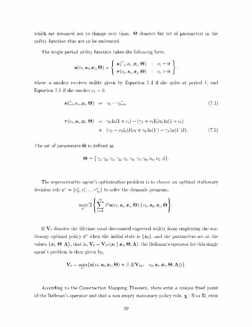
which are assumed not to change over time. � denotes the set of parameters in the
utility function that are to be estimated.
The single period utility function takes the following form,
u(ct; st;xi;�) =
(�(It; at;xi;�) : ct = 0
� (ct; si;xi;�) : ct > 0
);
where a smoker receives utility given by Equation 7.4 if she quits at period t, and
Equation 7.5 if she smokes ct > 0.
�(It; at;xi;�) = 5 + 6It; (7.4)
� (ct; si;xi;�) = 0 ln(1 + ct) + ( 1 + �1It)at ln(1 + ct)
+ ( 2 + �2It)Ptct + 3 ln(Y ) + 4 ln(Y )Pt: (7.5)
The set of parameters � is de�ned as
� = f 1; 2; 3; 4; 5; 6; 7; 8; �0; �1; �g:
The representative agent's optimization problem is to choose an optimal stationary
decision rule c� = fc�0; c�1; : : : c
�1g to solve the dynamic program,
maxc�
E
(1Xt=0
�tu(ct; st;xi;�) j c0; s0;xi;�
):
If Vt denotes the lifetime total discounted expected utility from employing the sta-
tionary optimal policy c� when the initial state is fs0g, and the parameters set at the
values fxi;�;�g, that is, Vt = Vc�(st j xi;�;�), the Bellman's operator for this single
agent's problem is then given by,
Vt = maxc�fu(ct; st;xi;�) + � E (Vt+1 j ct; st;xi;�;�))g:
According to the Constraction Mapping Theorem, there exist a unique �xed point
of the Bellman's operator and that a non-empty stationary policy rule, � : S 7! D , exist
39

of the form shown in Equation 7.6. Using the properties of the contraction mapping,
we can solve for the �xed point Vt by successive approximation methods and the policy
rule by policy improvement techniques.
c�t = argmaxc�
t
fu(ct; st;xi;�) + � E (Vt+1ct; st;xi;�;�)g
= �(st j xi;�;�) = �t, where c�t 2 [0; �C]; (7.6)
For each realization of the state vector st 2 S, the agent optimizes by comparing the
total lifetime expected utility from quitting versus continueing smoking. As with discrete
choice models, any identi�cation has to come from utility di�erence arising from this two
discrete options. The estimation cannot identify the actual level of utility from either
smoking or quitting but only the di�erence. The mean utility level in � (:) is normalized
to zero and the di�erence in mean utility is given by 5. 6 captures the utility di�erence
arising from quitting the previous period. The term 1 picks up the reinforcement e�ect
of addiction and together with 0 contributes to the marginal utility from consumption.
2 captures the disutility associated with price Pt. The variable log(Y ) is introduced
to capture the empirical fact higher income group individuals are more likely to quit.
The interaction term Pt log(Y ) captures price sensitivity across di�erent income groups.
The remaining � 0s parameters allow for marginal e�ects resulting from quitting in the
previous periods.
Estimation
The estimation strategy for this model is similar to that used in Section 4.4. A
Nested Fixed Point Maximum Likelihood Estimation method is used to estimate the
parameters of this model. The �xed point to the Bellman equation conditional on a set
of parameter estimates f�̂; �̂;xig is numerically computed using a modi�ed policy iter-
ation method. The mixed discrete and continuous optimal control is then solved using
Brent's numerical method over a discretized state space. Conditional on this set of pa-
rameters, a likelihood is assigned to an entire path of observed consumption conditional
on the observation in the �rst period. The structural restriction that the single period
utility function described in the previous section ensures that the policy funtion is weakly
monotonic in the unobserved at. The monotonicity property allows the unobserved ai,
corresponding to the observed ci > 0, to be solved through simple interpolation. Here,
I omit the details already discussed in Section 4.4. Readers should refer to that section
40

for a complete discussion of the estimation procedure.
Table D1 : MLE Estimates for preliminary model
Parameters Estimates Std. Error
1 0:557 0:045
2 �153:733 12:296
3 0:029 1:295
4 �0:073 5:960
5 0:093 10:490
6 0:237 13:269
�1 �0:054 4:471 � 10�3
�2 0:125 0:063
Æ0 �0:096 3:313 � 10�5
�� 13:389 3:901 � 10�3
Parameters exogenously estimated
�0 1:026 0.0128
Fixed parameters
� 0:9
Results
Table D1 shows the parameter estimates and their standard errors. These estimates
are for a subsample of smokers from the state of Massachusetts(MA). The parameter
estimates on most of the variables of interest conform to what we expect from the model.
The coeÆcient representing the reinforcement e�ect 1 is positive as expected and signif-
icantly di�erent from zero. The coeÆcient on price, 2, is signi�cant and negative. The
mean di�erence in utility level from quitting denoted by 5 (and 6 if the individual quit
the previous period) is not signi�cantly di�erent from 0. These estimates suggest that
there is no signi�cant di�erence in mean utility level from quitting and smoking. Reiter-
ating the point made earlier, addiction in this preliminary model is a desired `good' that
improves the marginal utility from future units of consumption. The only reason why
an individual would want to quit is the disutility he or she experience from the prices,
and the negative draw to the stochastic shock �t that lowers the stock of addiction such
that continued smoking is no longer as attractive.
41

The policy rule and the value function corresponding to these estimates are shown
in Figure 7.1. The policy rule is increasing in the level of addiction (at), while holding
prices constant and decreasing in prices (Pt) holding the addictive stock constant, as
shown in the Figure 7.1(c) and 7.1(e). Similarly, the shape of the value function also
follows what we intuitively expect. It is increasing in the addictive stock and decreasing
in prices as shown in Figures 7.1(d) and 7.1(f).
Insert Figure 7.1 here
To test this model consider how well it predicts the behavior observed in the data. Ta-
ble D2 below shows the bootstrap predictions of quit proportions for two income groups
in the state of Massachusetts. These predictions are calculated by drawing a bootstrap
sample from the observed empirical distribution for 1989. The observed behaviors are
then simulated according to the estimated policy rules and stochastic processes of the
model. The model under-predicts the proportions of quits each period by a large margin.
Though the predicted proportions increase over time, it does not re ect the behaviors
observed in the data.
Table D2 : Boot-strap quit predictions in % for income gp. Y2 and Y4
Years Income gp. 2 Income gp. 4
Predicted Observed Predicted Observed
1990 0.87 21.82 2.05 26.19
1991 1.23 24.24 2.45 30.95
1992 1.35 33.33 2.53 37.14
1993 1.53 33.94 2.70 43.33
Aside from this, the model also provides unrealistic estimates of the short-run price
elasticities. Table D3 shows the estimated short-run elasticities implied by the bootstrap
simulation. The two columns shows the implied elasticity arising from a given price
change in two separate scenarios. The �gures in the �rst column show the elasticity
at t = 1989 holding the distribution of cigarette consumption and stock of addiction
constant for individuals in the second income group, Y2.
42

Table D3 : Short Run price elasticity estimates at t = 1989 for Y2
% price Elasticity Estimates
change holding at constant allowing at to change
2 -9.03 0.02
3 -8.64 -5.29
5 -7.50 -6.45
10 -4.85 -4.53
15 -3.62 -3.45
The second considers a similar experiment allowing the stock of addiction to adjust
according to the estimated accumulation process. These elasticities are obviously in-
correct. The existing empirical literature has accepted the demand price elasticity for
smoking to be in the range of -0.4 to -0.8.
The data for the state of MA shows that around 25 percent of the smokers quit in
the �rst period and this proportion increases in each year of the sample. To match this
observed data, the model has to rely on �t to generate the distribution of consumption
each period and match the proportions of quits. The speci�cation of only two sources
of unobservables, �t that creates uncertainty about prices and �t that generates ran-
domness in the accumulation process, is not suÆcient to account for the dynamics in
the data. Because accumulating at only results in increased costs, smokers have little
incentive to quit. Instead the model predicts that smokers will gradually decrease con-
sumption as real prices increase over time. It attributes all of the decrease in smoking
to the price increases. The model reconciles the underprediction of quit percentages
by underpredicting the overall consumption of smokers, and gives estimates of mean
cigarette smoked that is well below what is observed. Because the model predicts that
smokers will gradually decrease consumption each period and attributes this to prices,
it generates upward biased elasticity estimates.
43

References
Ainslie, G., and N. Haslam (1992): \Hyperbolic Discounting," in Choice Over Time,
ed. by G. Loewenstein, and J. Elster. Russel Sage Foundation.
Akerlof, G. A. (1991): \Procrastination and Obedience," American Economic Re-
view, 81(2), 1{19.
Barnett, P., T.-W. Hu, H.-Y. Sung, and T. Keeler (1995): \The Impact of
California Anti-Smoking Legislation on Cigarette Sales, Consumption, and Prices,"
Tobacco Control, Summer(4), S34{S38.
Becker, G. S., M. Grossman, and K. M. Murphy (1994): \An Empirical Analysis
of Cigarette Addiction," American Economic Review.
Becker, G. S., and K. V. Murphy (1988): \A Rational Model of Addiction,"
Journal of Political Economy, 96(4), 675{700.
Behrman, J. R., R. C. Sickles, and P. Taubman (1990): \Age-Speci�c Death
Rates with Tobacco Smoking and Occupational Activity: Sensitivity to Sample
Length, Functional Form, and Unobserved Frailty," Demogaphy, 27(2), 267{284.
Chaloupka, F. J. (1991): \Rational addictive behavior and cigarette smoking," Jour-
nal of Political Economy, 99(4), 722{742.
Chaloupka, F. J., and H. Wechsler (June, 1997): \Price, Tobacco Control Policies
and Smoking Among Young Adults," Journal of Health Economics, 16(3), 359{373.
COMMIT Research Group (1996): \Community Intervention Trial for Smoking
Cessation (COMMIT): Summary Design and Intervention," Journal of the National
Cancer Institute, 83(22), 1620{1628.
(February 1995): \Community Intervention Trial for Smoking Cessation (COM-
MIT):I. Cohort Results from a Four Year Community Intervention," American Jour-
nal of Public Health, 85(2), 183{199.
Dockner, E. J., and G. Feichtinger (1993): \Cyclical Consumption Patterns and
Rational Addiction," American Economic Review, 83(1 March), 256{263.
Falba, T. (2000): \E�ects of Health Shocks on the Smoking Cessation or Middle Aged
Couples," Dept. of Epidemiology and Public Health, Yale University, mimeo.
44

Fethke, G., and R. Jagannathan (1996): \Habit persistence, heterogenous tastes,
and imperfect competition," Journal of Economic Dynamics and Control, 20, 1193{
1207.
Hitsch, G. (2000): \Estimating a Bayesian Learning Model of Product Launch and
Product Exit," Dept. of Economics, Yale University, mimeo.
Hu, T.-W., Q.-F. Ren, T. Keeler, and J. Bartlett (1995): \The Demand for
Cigarettes in California and Behavioral Risk Factors," Health Economics, 4, 7{14.
Hu, T.-W., H.-Y. Sung, and T. Keeler (1995): \The State Antismoking Campaign
and the Industry Response: The E�ects of Advertising on Cigarette Consumption in
California," A. E. R. Papers and Proceedings, 85(2), 85{90.
Hymowitz, N., M. Cummings, A. Hyland, W. Lynn, T. Pechacek, and
T. Hartwell (1997): \Predictors of smoking cessation in a cohort of adult smokers
followed for �ve years," Tobacco Control, suppl 2(6), S57{S62.
Jones, A. (1994): \Health, Addiction, Social Interaction and the decision to quit
smoking," Journal of Health Economics, 13, 93{110.
Lewit, E. M., and D. Coate (1982): \The potential for using Excise taxes to reduce
smoking," Journal of Health Economics, 1(December), 121{145.
Lucas, R. E., and N. L. Stokey (1989): Recursive Methods in Economic Dynamics.
Harvard University Press, Cambridge, MA.
National Cancer Institute (1995): Community Based Interventions for smokers:
The COMMIT Field Experience. US Dept. of Health of Human Services, National
Institute of Health.
(1997): Changes in Cigarette-Related Disease Risks and Their Implication for
Prevention and Control. US Dept. of Health of Human Services, National Institute of
Health.
O'Donoghue, T., and M. Rabin (1999): \Addiction and Self Control," in Addiction:
Entries and Exits, ed. by J. Elster, vol. 2. Russel Sage Foundation.
Orphanides, A., and D. Zervos (1995): \Rational Addiction with Learning and
Regret," Journal of Political Economy, 103(August), 739{58.
45

(1998): \Myopia and Addictive Behavior," The Economic Journal, 108(Jan-
uary), 75{91.
Pakes, A. (1996): \Dynamic Structural Models, Problems and Prospects: mixed con-
tinuous discrete controls and market interactions," in Advances in Econometrics, Sixth
World Congress, ed. by C. Sims, vol. 2, pp. 171{259.
Rabin, M. (1998): \Psychology and Economics," Journal of Economic Literature,
March(36), 11{46.
Ross, S. M. (1970): Applied Probability Models with Optimization Applications. Dover
Publications Inc.
Rust, J. (1994): \Structural Estimation of Markov Decision Processes," in Handbook
of Econometrics, ed. by R. F. Engle, and D. L. McFadden, vol. 4, pp. 3081{3143.
(1996): \Estimation of Dynamic Structural models, problems and prospects:
discrete decision processes," in Advances in Econometrics, Sixth World Congress, ed.
by C. Sims, vol. 2, pp. 119{170.
Shefrin, H. M. (1984): \Self-command in practice, in policy and in a theory of rational
choice," American Economic Review, 74(May), 1{11.
Showalter, M. H. (1999): \Firm Behavior in a Market with Addiction: The Case of
Cigarettes," Journal of Health Economics, 18, 409{427.
Smith, K., et al. (2000): \Do Smokers Respond to Health Shocks," Dept. of Health
policy and Management, Duke University, mimeo.
Stigler, G. J., and G. S. Becker (1977): \De Gustibus Non Est Disputandum,"
American Economic Review, March(67), 76{90.
Thaler, R., and H. M. Shefrin (1981): \An Economic Theory of Self-Control,"
Journal of Political Economy, 89(2), 392{406.
Timmins, C. (2000): \Measuring the Dynamic EÆciency Cost of regulator's preferences:
Municipal water utilities in the arid west," Econometrica, forthcoming.
Tobacco Institute (1994): The Tax Burden on Tobacco: Historical Compila-
tionTobacco Tax Council, Richmond VA.
46

US Dept. of Health of Human Services (1989): Reducing the Health Conse-
quences of Smoking: 25 Years of Progress. A Report of the Surgeon General., no.
(CDC 89-8411).
(1990): The Health Bene�ts of Smoking Cessation. A Report of the Surgeon
General., no. (CDC 90-8416).
Wasserman, J., W. G. Manning, J. P. Newhouse, and J. D. Winkler (1991):
\The e�ects of excise taxes and regulations on cigarette smoking," Journal of Health
Economics, 10, 43{65.
Wray, L., A. Herzog, R. Willis, and R. Wallace (1998): \The impact of Educa-
tion and Heart Attack on Smoking Cessation Among Middle-Aged Adults," Journal
of Health and Social Behavior, pp. 271{294.
47
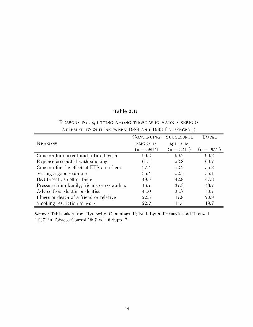
Table 2.1:
Reasons for quitting among those who made a serious
attempt to quit between 1988 and 1993 (in percent)
Continuing Successful Total
Reasons smokers quiters(n = 5807) (n = 3214) (n = 9021)
Concern for current and future health 90.2 90.2 90.2Expense associated with smoking 64.4 52.8 60.7Concern for the e�ect of ETS on others 57.4 52.2 55.8Setting a good example 56.4 52.4 55.1Bad breath, smell or taste 49.5 42.8 47.3Pressure from family, friends or co-workers 46.7 37.3 43.7Advice from doctor or dentist 44.0 33.7 40.7Illness or death of a friend or relative 22.3 17.8 20.9Smoking restriction at work 22.2 14.4 19.7
Source: Table taken from Hymowitz, Cummings, Hyland, Lynn, Pechacek, and Hartwell
(1997) in Tobacco Control 1997 Vol. 6 Supp. 2.
48

Table 3.1:
Smoking Prevalence and Quit
Rates from Sample Survey (Jan. 1988)
Smoking Percentage that Quit Sample Sample
Community Area Prev. the last more than that smoked Sizerate 5 yr. 5 yr. ago 100 cigs.
Hayward CA 23.5 19.8 28.3 4801 10504
Vallejo CA | 23.4 20.3 28.0 4854 10628
Peterborough, Ontario CAN 29.1 18.3 25.8 3390 6475
Brantford, Ontario CAN | 31.1 16.6 25.0 3260 6090
Cedar Rapids/Marion IA | 22.7 20.8 30.1 3890 8376
Davenport IA 24.9 19.8 28.4 3761 7769
Fitchburg/Leominster MA | 28.3 20.1 22.3 3830 7753
Lowell MA 26.2 19.4 27.9 3555 7118
Patterson NJ | 24.5 16.9 20.6 4798 12138
Trenton NJ 27.6 17.2 21.0 4746 10545
Las Cruces NM 18.7 21.6 32.4 6298 15434
Santa Fe NM | 20.3 23.5 33.8 8524 17826
Yonkers NY | 23.8 21.2 25.9 4599 10140
New Rochelle NY 23.6 21.2 26.5 5228 11486
Utica NY | 25.6 19.5 27.4 4200 8663
Binghamton/Johnson City NY 25.0 19.2 26.7 3921 8424
Greensboro NC 24.7 18.9 28.9 4444 9365
Raleigh NC | 21.1 21.6 28.3 4883 11559
Medford/Ashland OR | 20.0 19.1 37.5 5168 11154
Albany/Corvallis OR 18.1 20.1 33.5 4768 12161
Bellingham WA | 19.8 21.6 34.2 5911 13140
Longview/Kelso WA 24.7 19.0 31.9 3927 7749
| - Community randomised to receive intervention
49

Table 3.2:
Estimated and Observed Mortality risk ratio for white Female
(observed ratio from CPS I in parenthesis)
1-9 cigarettes a day
Duration in Years
Age 5-9 10-14 15-19 20-24 25-29 30-34
40-44 1.24 1.31 1.39 1.48 1.59 1.73
(1.01) (0.98) (1.55) (1.54) (1.76) (3.16)
45-49 1.20 1.26 1.32 1.38 1.46 1.56
(1.27) (1.75) (0.79) (1.70) (1.50) (1.59)
50-54 1.17 1.21 1.25 1.30 1.35 1.43
(0.46) (1.43) (1.51) (1.15) (1.22) (1.51)
55-59 1.14 1.18 1.21 1.24 1.27 1.32
(0.60) (1.12) (1.24) (0.87) (1.23) (1.13)
60-64 1.11 1.14 1.17 1.19 1.21 1.24
(1.06) (1.05) (0.92) (0.83) (0.92) (1.16)
20 cigarettes a day
Duration in Years
Age 5-9 10-14 15-19 20-24 25-29 30-34
40-44 1.39 1.63 1.89 2.21 2.64 3.25
( . ) (1.13) (2.49) (3.22) (2.57) (3.88)
45-49 1.34 1.53 1.72 1.92 2.19 2.56
( . ) (1.30) (1.68) (2.13) (1.81) (2.66)
50-54 1.30 1.45 1.59 1.72 1.88 2.09
(1.85) (1.14) (1.54) (1.68) (2.04) (1.96)
55-59 1.28 1.40 1.50 1.58 1.66 1.78
(2.05) (1.14) (1.31) (1.50) (1.43) (1.68)
60-64 1.26 1.37 1.44 1.48 1.52 1.57
(0.90) (1.43) (1.30) (1.27) (1.25) (1.75)
The mortality risk ratio is the ratio of the death rate of a smoker over that of a non-smoker.
The rates are expressed in number of deaths per 100,000 persons.
50

Table 3.3:
Cross-sectional 2SLS Regression instrumenting for ln(Pt)
Dependent Variable : ln(1 + Ct)
1989 1991 1993
Variables Est. t ratio Est. t ratio Est. t ratio
^ln(Pt) -0.062 -0.95 -0.251 -1.56 -0.370 -2.44
I2 -0.023 -0.73 -0.016 -0.24 -0.035 -0.50
I3 0.022 0.72 -0.024 -0.36 -0.140 -1.96
I4 0.039 1.22 -0.043 -0.63 -0.185 -2.52
Age 0.007 8.78 -0.000 -0.17 -0.005 -2.85
Starting Age -0.029 -15.72 -0.036 -9.15 -0.035 -8.16
Intv. -0.021 -1.38 -0.092 -2.84 -0.049 -1.40
Female -0.143 -8.60 -0.080 -2.24 -0.018 -0.46
Clerical 0.015 0.72 0.029 0.64 0.034 0.69
Tradesman 0.041 1.88 0.066 1.40 0.092 1.83
Unclas. 0.099 1.44 0.216 1.46 0.353 2.21
Homemaker 0.071 2.42 0.074 1.17 0.041 0.60
Student -0.048 -0.89 -0.134 -1.15 -0.093 -0.74
College -0.059 -3.40 -0.026 -0.71 -0.007 -0.18
Post Grad. -0.115 -3.57 -0.161 -2.31 -0.137 -1.82
constant 3.221 18.64 2.469 6.05 2.079 5.25
�R2 0.07 0.02 0.02
Key : Omitted occupation and education dummy variable is that for professionals and
individuals who didn't complete high school respectively. Total number of observations =
6902.
51

Table 3.4:
Cross-sectional Probit Regression instrumenting for ln(Pt)
Dependent Variable : Qt
1990 1993
Variables Est. t ratio Est. t ratio
^ln(Pt) 0.270 1.88 0.350 2.53
I2 -0.041 -0.56 0.020 0.30
I2 -0.010 -0.14 0.138 2.08
I2 0.050 0.67 0.170 2.50
Age 0.001 0.47 0.007 4.55
Starting Age 0.013 3.14 0.019 5.08
Intv. 0.034 0.95 0.035 1.12
Female -0.066 -1.70 -0.089 -2.53
Clerical -0.079 -1.59 -0.051 -1.15
Tradesman -0.073 -1.44 -0.062 -1.36
Unclas. -0.242 -1.40 -0.348 -2.20
Homemaker -0.071 -1.03 0.001 0.02
Student -0.088 -0.68 0.030 0.26
College 0.045 1.09 -0.031 -0.84
Post Grad. 0.101 1.36 0.064 0.95
constant -0.462 -1.22 -0.327 -0.90
% correctly predicted 81.54 68.91
% who quits in sample 18.5 31.0
Key : Omitted occupation and education dummy variable is that for professionals and
individuals who didn't complete high school respectively. Total number of observations =
6902.
52

Table 5.1:
Parameter values used in simulation
Parameter
values
Parameters 0 1:71of the utility 1 0:98function. 2 �195:50
3 0:40 4 0:30 5 100:00
Parameters Æ0 �0:21of the addiction Æ1 1:10process. �� 17:8
Parameters of the 0 0:80transition prob. for Ht+1 2 �10:00given Ht = hH,ie. 3 �0:01}H(Ht+1 j Ht = hH) 4 0:80
5 0:30
Parameters of the !0 �0:11transition prob. for Ht+1 !2 2:00given Ht = hL,ie. !3 9:90}H(Ht+1 j Ht = hL) !4 �0:02
!5 �0:01� 40:00
Fixed parameters
� 0:9
mi 0:005
53

Figure 7.1:
54