1 exercise 10 &11 one-compartmental model: simultaneous iv, oral and im dosing for a new...
Post on 20-Dec-2015
229 views
TRANSCRIPT
1
Exercise 10 &11One-compartmental model: Simultaneous IV , oral and
IM dosing for a new antibiotic in pigs
2
Exercise 10 &11:Overall objectives
• The ultimate goal of the present exercise is to show how to use PK and PD concepts to develop rationally a new antibiotic in pigs (exercise 11)
3
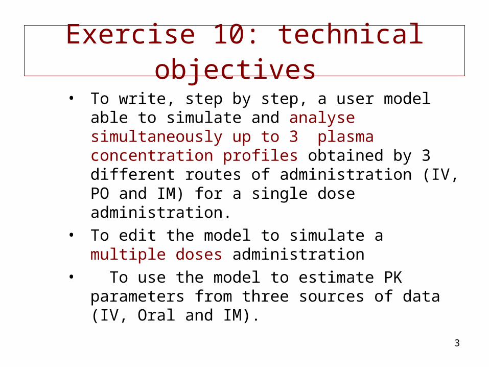
Exercise 10: technical objectives • To write, step by step, a user model able to
simulate and analyse simultaneously up to 3 plasma concentration profiles obtained by 3 different routes of administration (IV, PO and IM) for a single dose administration.
• To edit the model to simulate a multiple doses administration
• To use the model to estimate PK parameters from three sources of data (IV, Oral and IM).

4
Exercise 11: biological question to solve with the model
• Using Monte Carlo Simulations, to prospectively assess a possible dosage regimen for the IM formulation in order to be above a critical MIC in 90% of a pig population.
• To assess the target attainment rate (TAR) for the selected dose given the actual MIC distribution i.e. you have to compute the percentage of the pigs in the population that actually achieved the targeted objective
5
Problem specification (1)
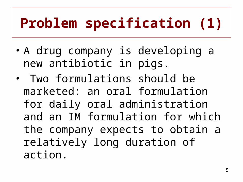
• A drug company is developing a new antibiotic in pigs.
• Two formulations should be marketed: an oral formulation for daily oral administration and an IM formulation for which the company expects to obtain a relatively long duration of action.
6
Problem specification (2)
• This antibiotic is a time-dependent antibiotic on Gram positive pathogens but a concentration-dependent antibiotic on Gram negative pathogens.
• For a time-dependent pathogen, the PK/PD criteria to be optimised is the time the plasma concentration remains above a critical plasma concentration and it is for this indication that the company is developing the IM long-acting formulation. Its objective is to be above a critical plasma concentration for at least 50% of the dosing interval (48h) in 90% of the pigs.
• For the Gram positive pathogens, the PK/PD criterion to optimise is the 24h ratio AUC/MIC in steady state condition with a target value equal to 125h. The oral formulation is developed for those pathogens.
7
Problem specification (3)
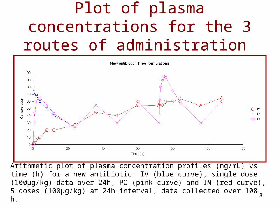
• The company carried out some pilot kinetics by IV, oral and IM route after a single (IV) or a multiple (PO, IM) doses administration. These preliminary data were obtained with a microdose of 100 µg/kg and are shown in figure 1
8
Plot of plasma concentrations for the 3 routes of administration
Arithmetic plot of plasma concentration profiles (ng/mL) vs time (h) for a new antibiotic: IV (blue curve), single dose (100µg/kg) data over 24h, PO (pink curve) and IM (red curve), 5 doses (100µg/kg) at 24h interval, data collected over 108 h.

9
10
Preliminary data analysis in WNL
• IV data are to be analysed by a mono-compartmental model without weighting factor

11
Preliminary data analysis in WNL
– Import data in WNL; edit headers and units – After excluding PO and IM data from the data
sheet (using Data>exclude>criteria), the IV data were analysed by a mono-compartmental model without weighting factor

12
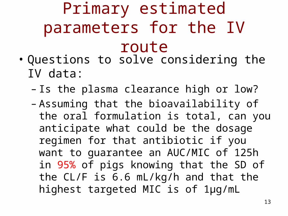
Primary estimated parameters for the IV route
13
Primary estimated parameters for the IV route
• Questions to solve considering the IV data:– Is the plasma clearance high or low?– Assuming that the bioavailability of the oral
formulation is total, can you anticipate what could be the dosage regimen for that antibiotic if you want to guarantee an AUC/MIC of 125h in 95% of pigs knowing that the SD of the CL/F is 6.6 mL/kg/h and that the highest targeted MIC is of 1µg/mL
14
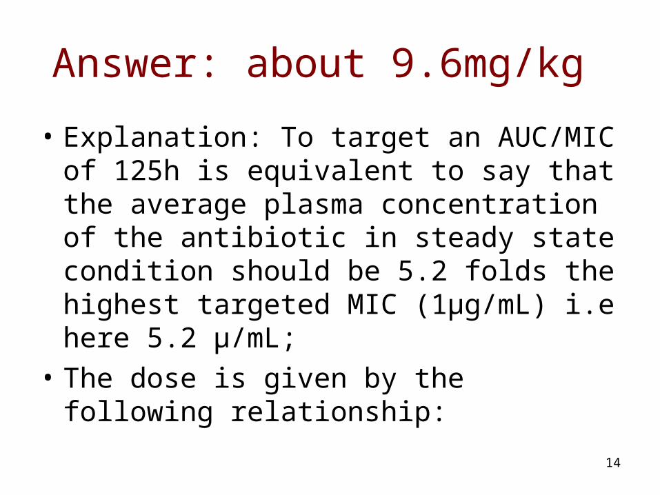
Answer: about 9.6mg/kg
• Explanation: To target an AUC/MIC of 125h is equivalent to say that the average plasma concentration of the antibiotic in steady state condition should be 5.2 folds the highest targeted MIC (1µg/mL) i.e here 5.2 µ/mL;
• The dose is given by the following relationship:
15
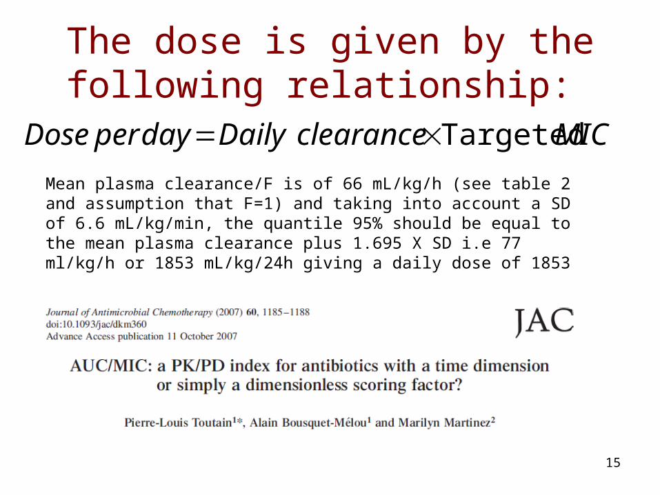
The dose is given by the following relationship:
MICclearanceDailydayperDose TargetedMean plasma clearance/F is of 66 mL/kg/h (see table 2 and assumption that F=1) and taking into account a SD of 6.6 mL/kg/min, the quantile 95% should be equal to the mean plasma clearance plus 1.695 X SD i.e 77 ml/kg/h or 1853 mL/kg/24h giving a daily dose of 1853 X 5.2 of 9640µg/kg/day or about 10 mg/kg

16
Fitting of the oral route (first 24h)
17
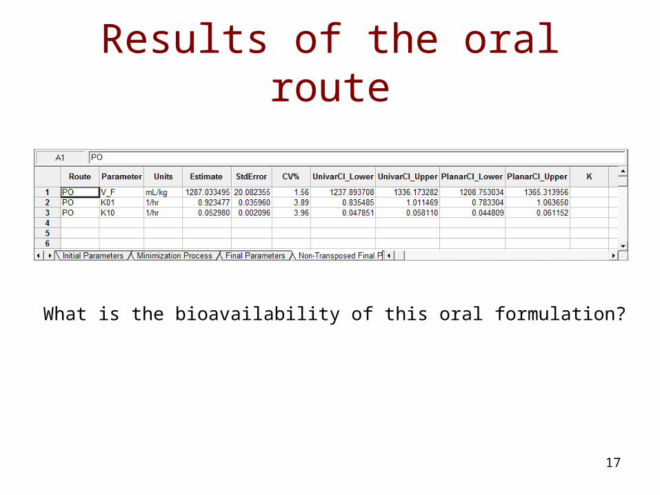
Results of the oral route
What is the bioavailability of this oral formulation?

18
The IM curve• For the IM route (first 24h) it was impossible to fit
the curve due to its shape over the first 24h.

19
The simultaneous fitting of the 3 curve• Rather than attempting to analyse separately each curve, it was
decided to fit simultaneously the three curves together because data were collected in the same animal.
• The advantage of this approach is to obtain more accurate and precise parameter estimates.
• For example, a common K10 can be estimated from the 3 curves allowing to estimate without ambiguity the different rate constants of absorption for the oral and IM routes of administration,
• the model can include a bioavailability factor to estimate for each formulation,
• and if data are inappropriate to properly characterise a curve as it is the case here for the IM formulation over the first 24 h, information available from other curves can be very helpful
20
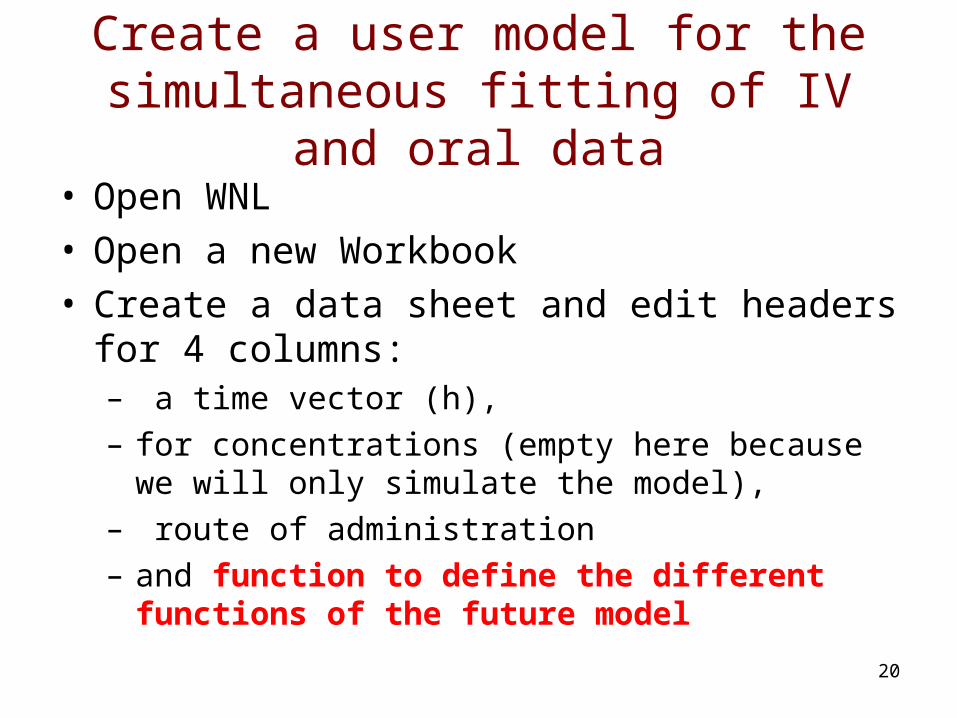
Create a user model for the simultaneous fitting of IV and oral data
• Open WNL• Open a new Workbook• Create a data sheet and edit headers for 4
columns:– a time vector (h), – for concentrations (empty here because we will only
simulate the model),– route of administration – and function to define the different functions of
the future model
21
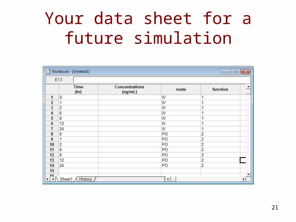
Your data sheet for a future simulation

22
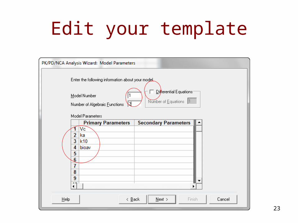
Open template to build an user model
23
Edit your template

24
The template as edited by WNL
25
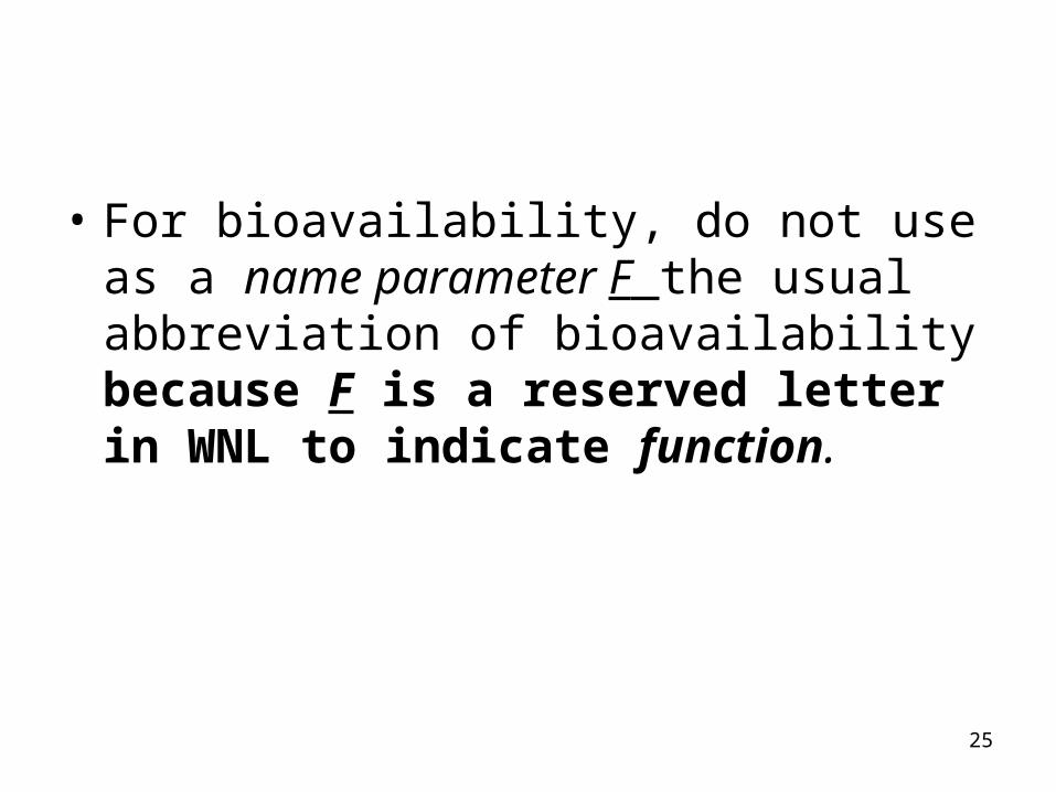
• For bioavailability, do not use as a name parameter F the usual abbreviation of bioavailability because F is a reserved letter in WNL to indicate function.
26
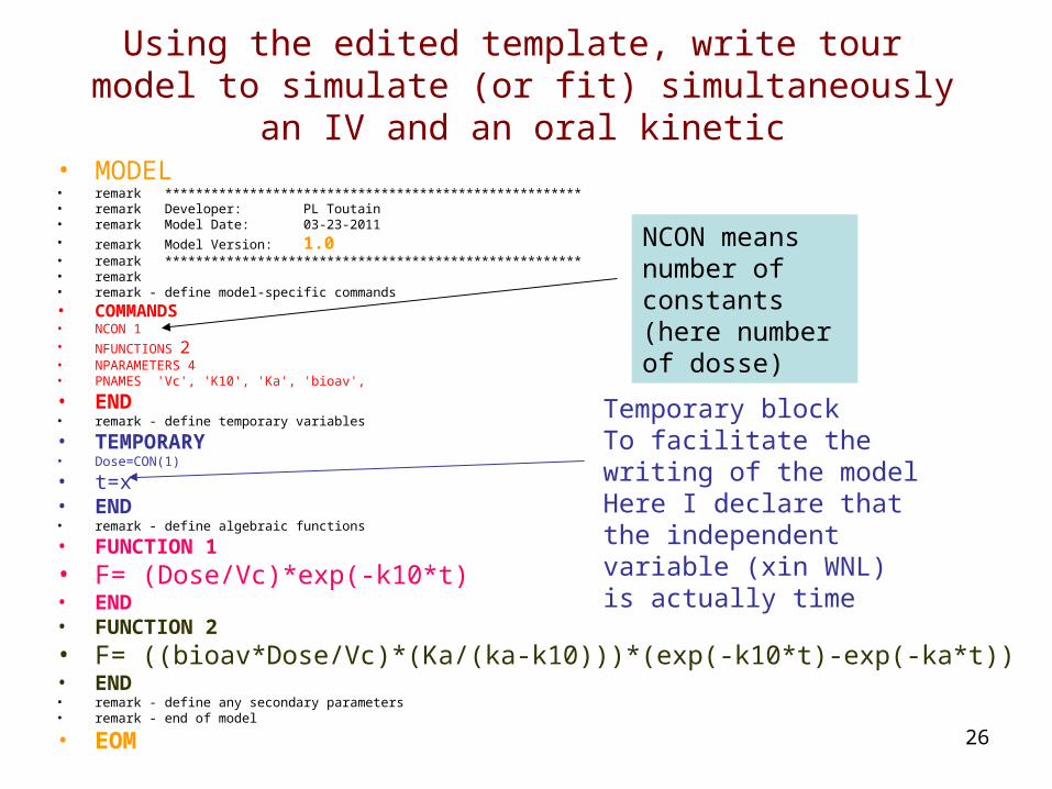
Using the edited template, write tour model to simulate (or fit) simultaneously an IV and an oral kinetic
• MODEL• remark ******************************************************• remark Developer: PL Toutain• remark Model Date: 03-23-2011• remark Model Version: 1.0• remark ******************************************************• remark• remark - define model-specific commands
• COMMANDS• NCON 1 • NFUNCTIONS 2• NPARAMETERS 4• PNAMES 'Vc', 'K10', 'Ka', 'bioav',
• END• remark - define temporary variables
• TEMPORARY • Dose=CON(1)
• t=x• END • remark - define algebraic functions
• FUNCTION 1
• F= (Dose/Vc)*exp(-k10*t)• END• FUNCTION 2
• F= ((bioav*Dose/Vc)*(Ka/(ka-k10)))*(exp(-k10*t)-exp(-ka*t))• END• remark - define any secondary parameters• remark - end of model
• EOM
NCON means number of constants (here number of dosse)
Temporary blockTo facilitate the writing of the modelHere I declare that the independent variable (xin WNL) is actually time

27
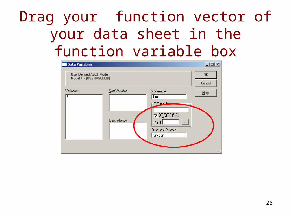
Run your model to simulate
• After having completed your model, you can proceed with the WNL interface, defining the X variable (Time).
• We have no Y variable (no experimental data) because we are only simulating. The field Function variable should be filled with the name of the corresponding column (here named function in our data sheet) and the radio button Simulate data should be ticked.
28
Drag your function vector of your data sheet in the function variable box
29
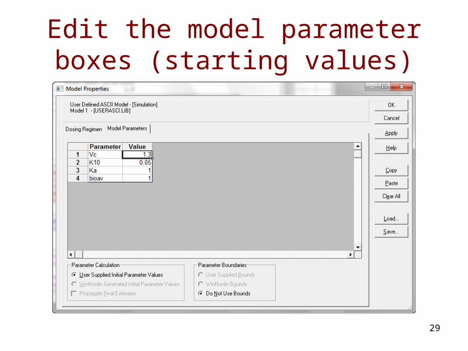
Edit the model parameter boxes (starting values)

30
Edit the dosage regimen box (dose)
31
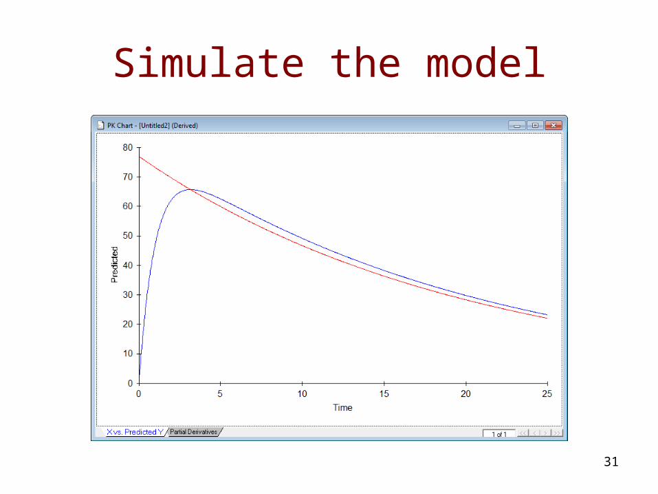
Simulate the model

32
Question: At what time the PO curve crosses the IV curve
and is it the Tmax/Cmax of the PO curve?
• To answer this question, you can inspect the sheet Predicted data of the workbook and search the times for which functions 1 and 2 are equal i.e. about 51 min that is also the Tmax/Cmax of the oral curve.

33

34
Question: At what time the PO curve crosses the IV curve
and is it the Tmax/Cmax of the PO curve?
• A better approach would consist in analyzing these predicted data with the WNL NCA module
• and an even better approach to answer the question is to use the model to compute these secondary parameters as it is the objective of the next refined model.
35
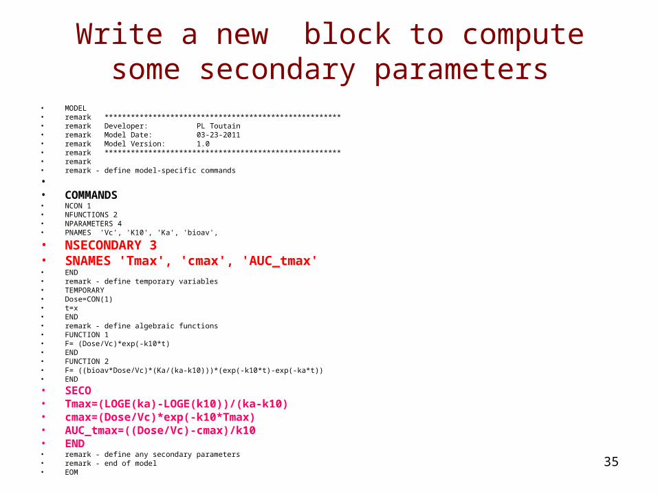
Write a new block to compute some secondary parameters
• MODEL• remark ******************************************************• remark Developer: PL Toutain• remark Model Date: 03-23-2011• remark Model Version: 1.0• remark ******************************************************• remark• remark - define model-specific commands
• • COMMANDS• NCON 1 • NFUNCTIONS 2• NPARAMETERS 4 • PNAMES 'Vc', 'K10', 'Ka', 'bioav',
• NSECONDARY 3• SNAMES 'Tmax', 'cmax', 'AUC_tmax'• END• remark - define temporary variables• TEMPORARY • Dose=CON(1)• t=x• END • remark - define algebraic functions• FUNCTION 1• F= (Dose/Vc)*exp(-k10*t)• END• FUNCTION 2• F= ((bioav*Dose/Vc)*(Ka/(ka-k10)))*(exp(-k10*t)-exp(-ka*t))• END
• SECO• Tmax=(LOGE(ka)-LOGE(k10))/(ka-k10)• cmax=(Dose/Vc)*exp(-k10*Tmax)• AUC_tmax=((Dose/Vc)-cmax)/k10• END• remark - define any secondary parameters• remark - end of model• EOM
36
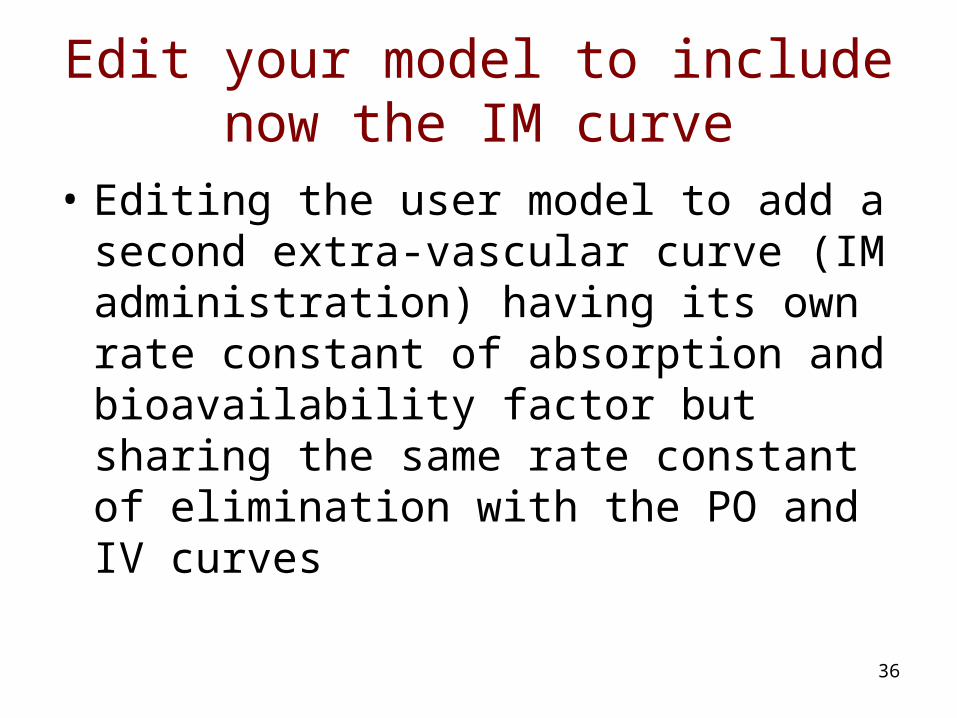
Edit your model to include now the IM curve
• Editing the user model to add a second extra-vascular curve (IM administration) having its own rate constant of absorption and bioavailability factor but sharing the same rate constant of elimination with the PO and IV curves
37
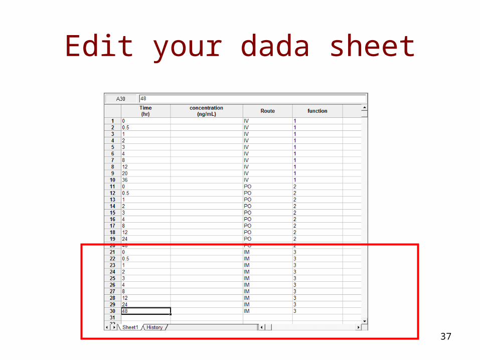
Edit your dada sheet
38
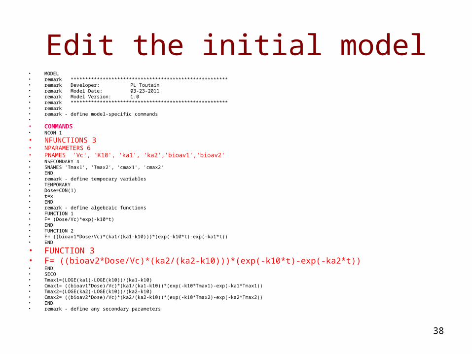
Edit the initial model• MODEL• remark ******************************************************• remark Developer:PL Toutain• remark Model Date: 03-23-2011• remark Model Version: 1.0• remark ******************************************************• remark• remark - define model-specific commands • • COMMANDS• NCON 1
• NFUNCTIONS 3• NPARAMETERS 6• PNAMES 'Vc', 'K10', 'ka1', 'ka2','bioav1','bioav2'• NSECONDARY 4• SNAMES 'Tmax1', 'Tmax2', 'cmax1', 'cmax2'• END• remark - define temporary variables• TEMPORARY • Dose=CON(1)• t=x• END • remark - define algebraic functions• FUNCTION 1• F= (Dose/Vc)*exp(-k10*t)• END• FUNCTION 2• F= ((bioav1*Dose/Vc)*(ka1/(ka1-k10)))*(exp(-k10*t)-exp(-ka1*t))• END
• FUNCTION 3• F= ((bioav2*Dose/Vc)*(ka2/(ka2-k10)))*(exp(-k10*t)-exp(-ka2*t))• END• SECO• Tmax1=(LOGE(ka1)-LOGE(k10))/(ka1-k10)• Cmax1= ((bioav1*Dose)/Vc)*(ka1/(ka1-k10))*(exp(-k10*Tmax1)-exp(-ka1*Tmax1))• Tmax2=(LOGE(ka2)-LOGE(k10))/(ka2-k10)• Cmax2= ((bioav2*Dose)/Vc)*(ka2/(ka2-k10))*(exp(-k10*Tmax2)-exp(-ka2*Tmax2))• END• remark - define any secondary parameters
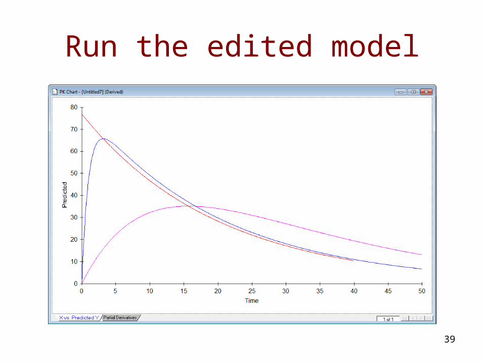
39
Run the edited model

40
Editing the user model to simulate a multiple dose administration: the new
command block
• comm • NCON 11• nparm 6• • pnames 'vc', 'k10', 'ka1',
'Ka2','bioav1','bioav2'• • nfun 3• end
NCON 11 indicates that to define your dosage regimen you need 11 constants
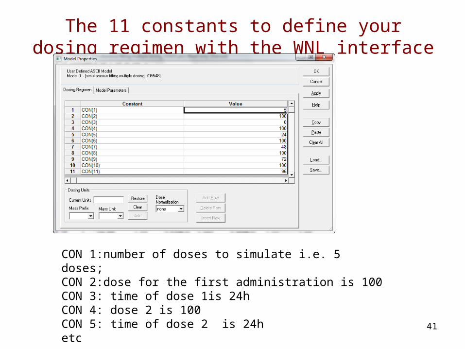
41
The 11 constants to define your dosing regimen with the WNL interface
CON 1:number of doses to simulate i.e. 5 doses; CON 2:dose for the first administration is 100 CON 3: time of dose 1is 24h CON 4: dose 2 is 100CON 5: time of dose 2 is 24hetc
42
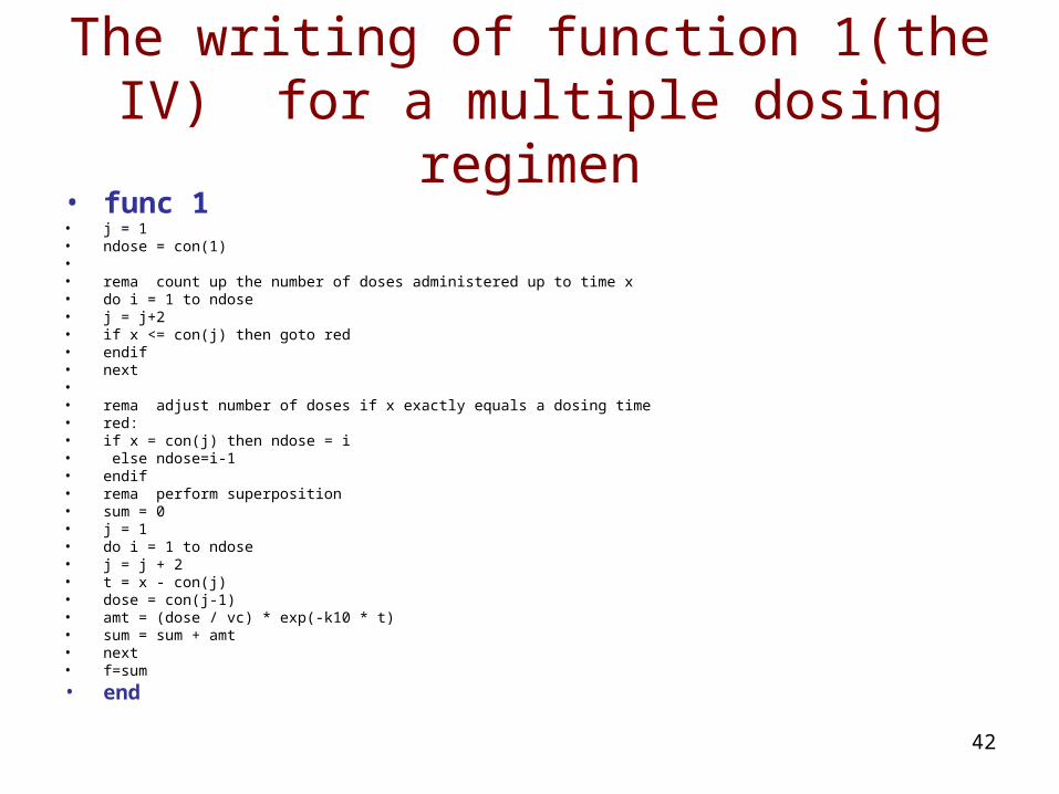
The writing of function 1(the IV) for a multiple dosing regimen
• func 1• j = 1• ndose = con(1)• • rema count up the number of doses administered up to time x• do i = 1 to ndose• j = j+2• if x <= con(j) then goto red• endif• next• • rema adjust number of doses if x exactly equals a dosing time• red:• if x = con(j) then ndose = i• else ndose=i-1• endif • rema perform superposition• sum = 0• j = 1 • do i = 1 to ndose• j = j + 2• t = x - con(j)• dose = con(j-1)• amt = (dose / vc) * exp(-k10 * t)• sum = sum + amt• next • f=sum
• end
43
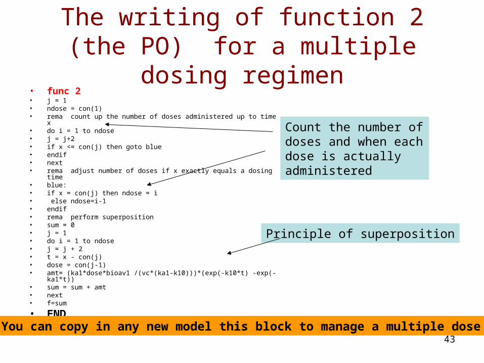
The writing of function 2 (the PO) for a multiple dosing regimen
• func 2• j = 1• ndose = con(1) • rema count up the number of doses administered up to time x• do i = 1 to ndose• j = j+2• if x <= con(j) then goto blue• endif• next • rema adjust number of doses if x exactly equals a dosing time• blue:• if x = con(j) then ndose = i• else ndose=i-1• endif • rema perform superposition• sum = 0• j = 1 • do i = 1 to ndose• j = j + 2• t = x - con(j)• dose = con(j-1)• amt= (ka1*dose*bioav1 /(vc*(ka1-k10)))*(exp(-k10*t) -exp(-ka1*t))• sum = sum + amt• next• f=sum
• END
Count the number of doses and when each dose is actually administered
Principle of superposition
You can copy in any new model this block to manage a multiple dose

44
Simulate a multiple dose administration

45
Fitting my raw data with my user model

46
Exercise 11(after the break)
47
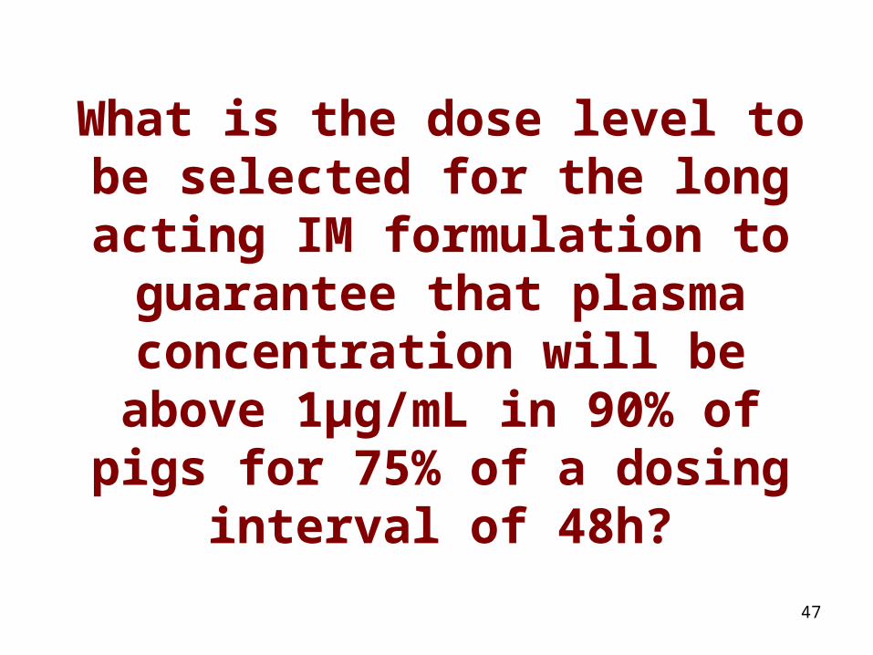
What is the dose level to be selected for the long acting IM formulation to guarantee that plasma concentration will be
above 1µg/mL in 90% of pigs for 75% of a dosing interval of 48h?
48
The question
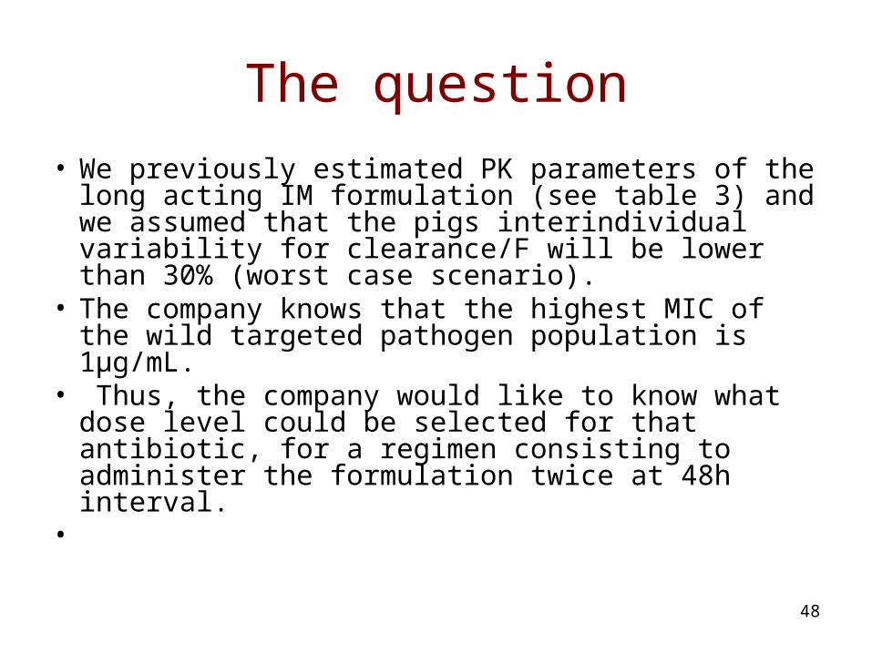
• We previously estimated PK parameters of the long acting IM formulation (see table 3) and we assumed that the pigs interindividual variability for clearance/F will be lower than 30% (worst case scenario).
• The company knows that the highest MIC of the wild targeted pathogen population is 1µg/mL.
• Thus, the company would like to know what dose level could be selected for that antibiotic, for a regimen consisting to administer the formulation twice at 48h interval.
•

49
The solution
• As it is a time dependent antibiotic, the PK/PD predictive surrogate is the time spent above a critical free plasma concentration corresponding to the MIC of interest (1µg/mL).
• Good clinical results are expected if the selected dose is able to be above the critical MIC for at least 50% of the dosage interval.
• As here the formulation is for a 48h dosing interval, we decided to determine a dose for which the time spent above 1µg/mL should be of 36h over the first 48h.– 36h: 24h for the first interval and 50% for the second dose
• To solve this question, the best approach is to perform some Monte Carlo Simulation (MCS).

50
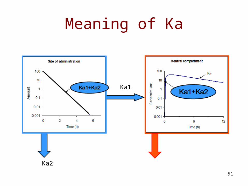
Write your PK model in an Excel sheet (write F% in terms of ka1 and Ka2)
51
Meaning of Ka
Ka2
Ka1
52
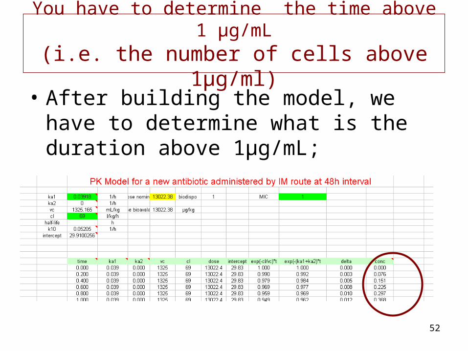
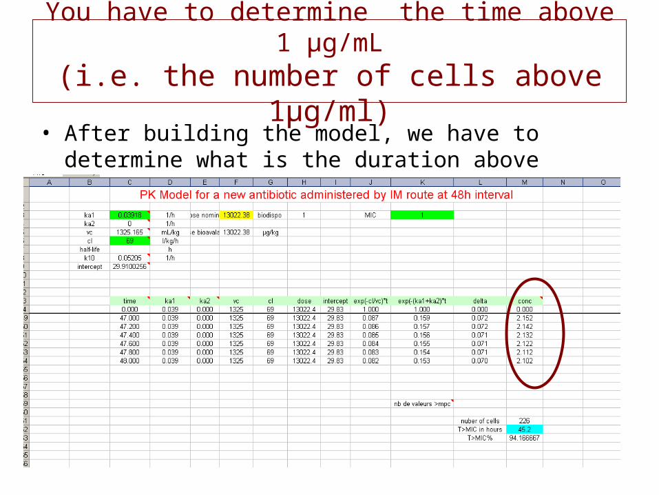
You have to determine the time above 1 µg/mL(i.e. the number of cells above 1µg/ml)
• After building the model, we have to determine what is the duration above 1µg/mL;
53
You have to determine the time above 1 µg/mL(i.e. the number of cells above 1µg/ml)
• After building the model, we have to determine what is the duration above 1µg/mL;
54
You have to determine the time above 1 µg/mL(i.e. the number of cells above 1µg/ml)
• After building the model, we have to determine what is the duration above 1µg/mL;
• this is easily obtained using the Excel (French) function = NB.SI(M15:M254;">1").
• Count cells that match criteria – COUNTIF
55
You have to count the time above 1 µg/mL(i.e. the number of cells above 1µg/ml)
• In Excel, count cells that meet a specific criterion. In this example the concentration above 1µg/mL will be counted.
• Select the cell in which you want to see the count (cell M261 in this example)
• Type an equal sign (=) to start the formula • Type: COUNTIF( • Select the cells that contain the values to check for the criterion. In
this example, cells M15 :M254 will be checked • Type a comma, to separate the arguments • Type the criterion. In this example, you're checking for plasma
concentration above 1µg/mL so type >1 in double quotes: ">1" or “>=1”
56
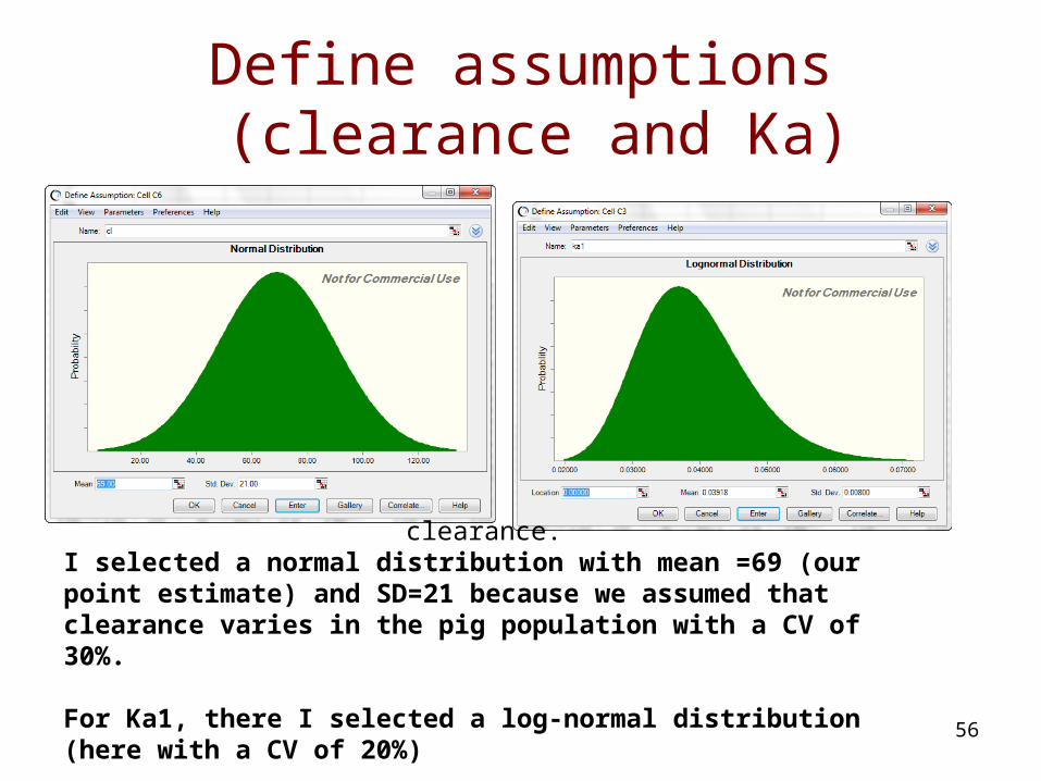
Define assumptions (clearance and Ka)
clearance.I selected a normal distribution with mean =69 (our point estimate) and SD=21 because we assumed that clearance varies in the pig population with a CV of 30%. For Ka1, there I selected a log-normal distribution (here with a CV of 20%)

57
Define forecast cells.
• Forecast cells contain the formula that refer to what we want to know i.e. time above 1µg/mL in cell M262.
• Click cell 262, click the toolbar button and the next window appears
58
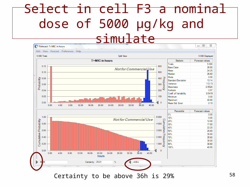
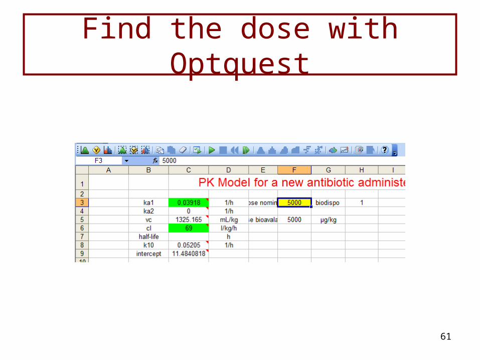
Select in cell F3 a nominal dose of 5000 µg/kg and simulate
Certainty to be above 36h is 29%
59
Determination of certainty
• The forecast chart can be obtained (you have to play with the ‘certainty grabber’).
• It is said that only 29.01% of pigs are able to achieve a time above 1µg/mL for at least 36h with a dose of 5000 µg/kg.
60
How to find the dose?
• To find the appropriate dose, we can repeat simulations until we find the dose for which 90% of pigs are covered.
61
Find the dose with Optquest
62
Find the dose with Optquest
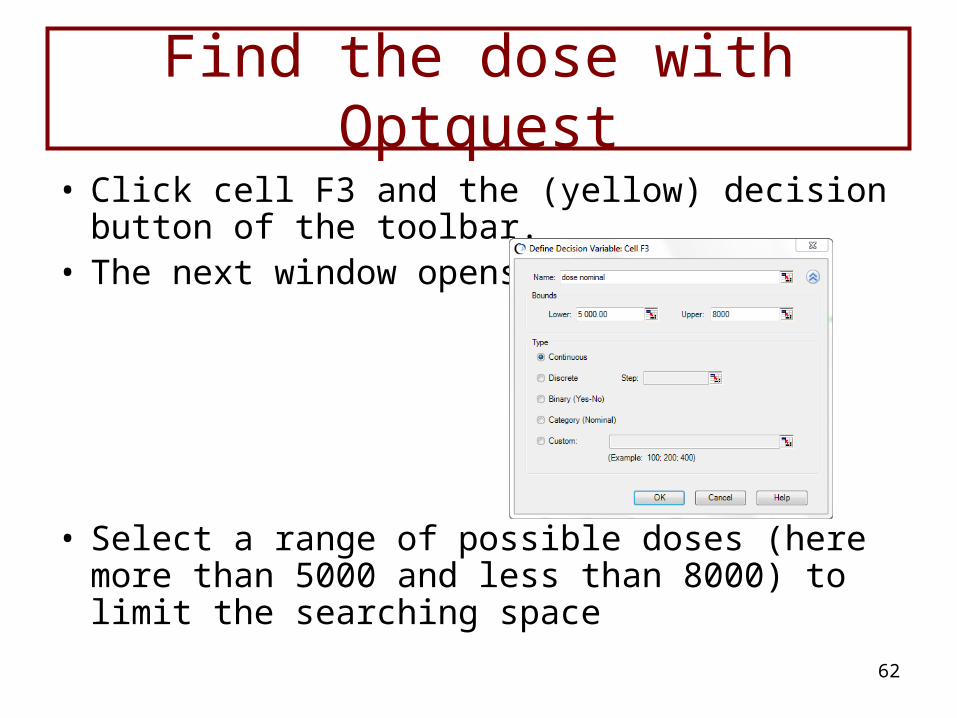
• Click cell F3 and the (yellow) decision button of the toolbar.
• The next window opens.
• Select a range of possible doses (here more than 5000 and less than 8000) to limit the searching space

63
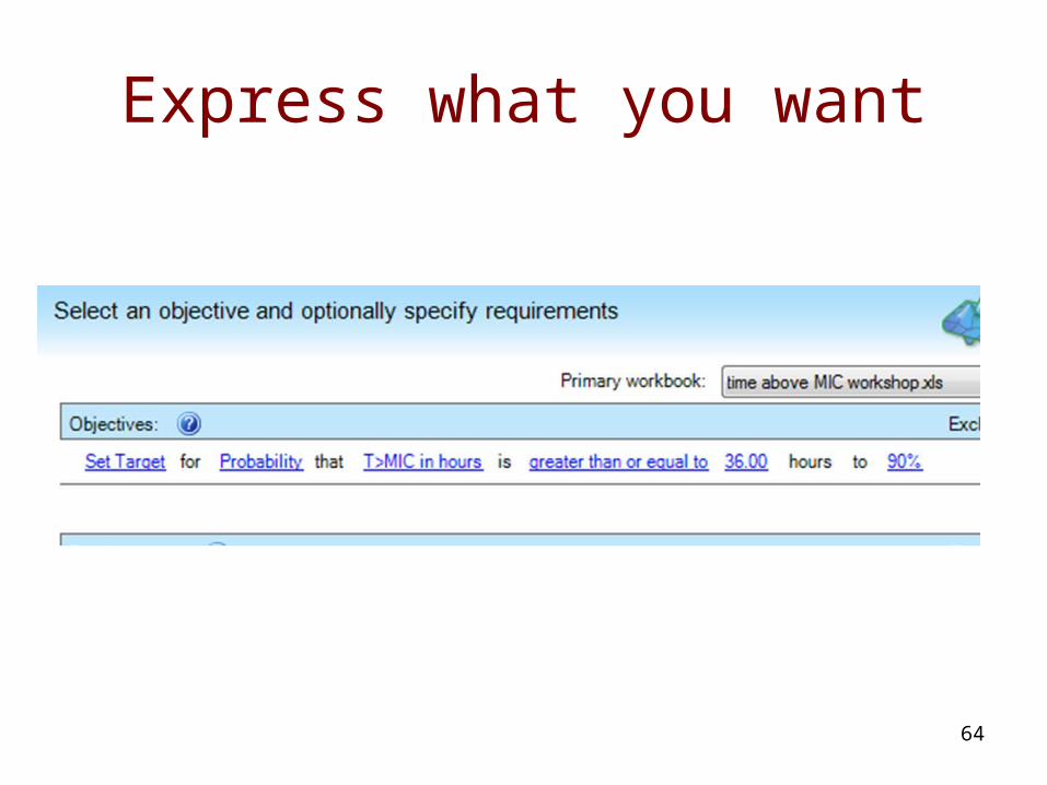
To express what you want
• Click the OptQuest button
64
Express what you want
65
OptQuest results
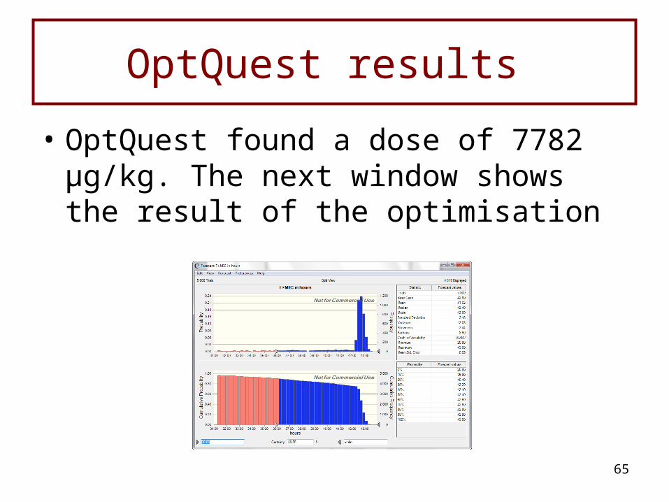
• OptQuest found a dose of 7782 µg/kg. The next window shows the result of the optimisation

66
Question: what will be the percentage of pigs for which the
plasma concentration will be higher than the different MICs collected in the field for at last 36h and for a standard dose of
10 mg/kg?
67
Empirical antibiotherapy
• The use of antibiotics is said empirical when initiated in the absence of microbiology results or even in the absence of a definitive diagnosis of infection.
• The only information available is the distribution of MICs for a given pathogen.
• As an example, the next table gives a MIC distribution and I assume that the probability a pig faces a pathogen is proportional to the frequency of these MIC (i.e. the likelihood for a pig to be infected with a pathogen having a MIC of 0.2 µg/ml is 3 times lesser than to be infected with a pathogen having a MIC of 0.5 µg/ml but equal to the probability to be infected with a pathogen having a MIC of 0.1µg/mL
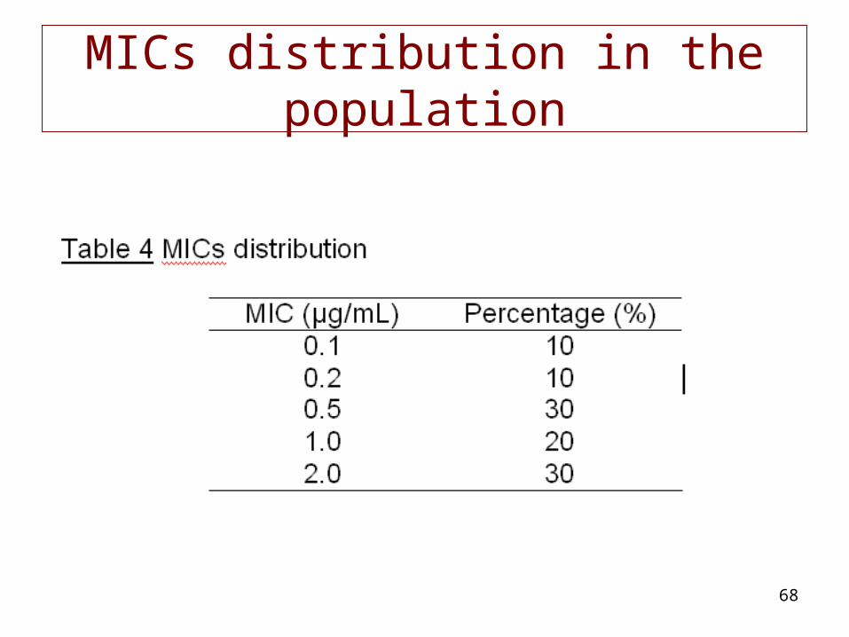
68
MICs distribution in the population
69
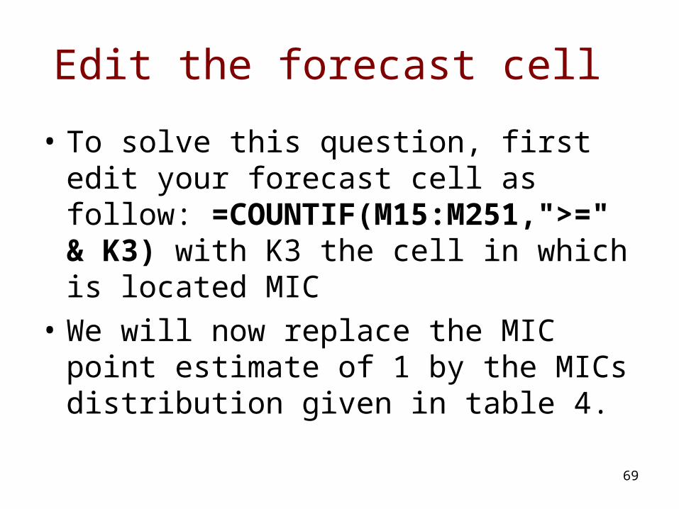
Edit the forecast cell
• To solve this question, first edit your forecast cell as follow: =COUNTIF(M15:M251,">=" & K3) with K3 the cell in which is located MIC
• We will now replace the MIC point estimate of 1 by the MICs distribution given in table 4.
70
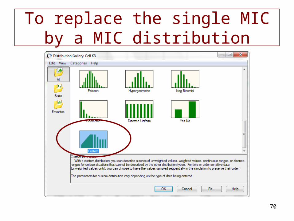
To replace the single MIC by a MIC distribution
71
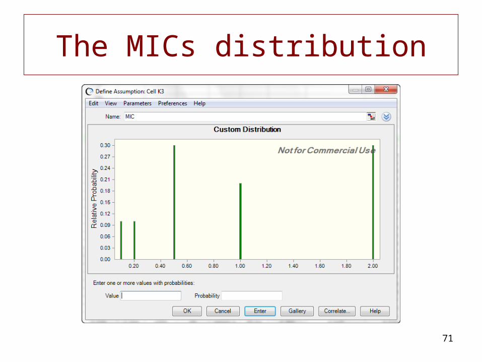
The MICs distribution

72
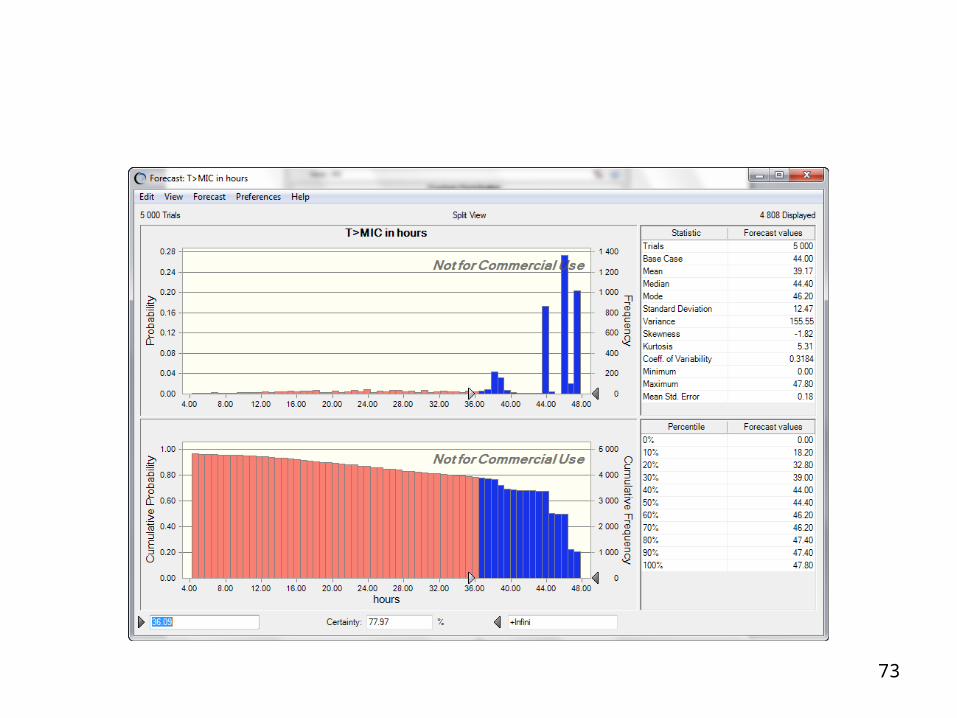
Simulate the model with the MICs distribution
• Results are shown in the next window: it appears that with a dose of 10 mg/kg, the TAR for 36h above the MIC is no longer of 90% but of 77.97%. Inspection of the upper panel clearly indicates a discrete distribution
73

74
Compute the dose with Optquest to guarantee that 90% of pigs will be
above a MIC of 1µg/mL for 36h over the 48h treatment
• Again we can require OptQuest to find the dose to suit our expectation. The dose found by OptQuest was 13.022mg/kg.