1

Number 332 January 13, 2012

1. Examine soils for signs of compaction __________________________________________ 1

2. Beneficial effects of earthworms on soils ________________________________________ 3

3. Clarification of topramezone (Impact/Armezon) marketing agreements _______________ 5

4. Comparative Vegetation Condition Report: December 27 – January 9 ________________ 5 1. Examine soils for signs of compaction Soil temperatures are hovering above freezing across much of Kansas right now (http://wdl.agron.ksu.edu/), making this a good time to get out and investigate soil profiles for signs of compaction. There is much you can learn by pushing a tile or soil probe into the ground. First, if you have never done so, you can learn something about the soil profile. How many inches of topsoil do you have? At what depth do you encounter changes in soil textures? Topsoil thickness and soil texture are two properties you can’t really control, at least not in the short term. One thing you can certainly look for and work on improving, however, is the density of your soil and whether there are any layers of compaction. Scientific approach: Density refers to the mass of a substance divided by its volume. In soil, we measure density (which we call bulk density) by pounding a cylinder of a known volume into the soil, and then drying the soil for two days in an oven. This gives us the oven dry mass, which we divide by the volume, and thus have the bulk density. There are detailed instructions available for this procedure online at http://soils.usda.gov/sqi/assessment/test_kit.html In scientific research, this method is used to analyze the effects of different management practices on soil quality, the differences between soil types, and other factors. It can also be used to quantify the differences in soil density at various depths within the soil, which helps in research on soil compaction. Hands-on approach: The scientific approach is not especially useful for producers and others to find compaction layers in their soils, however. There are much easier methods, with a level of precision that is good enough for practical use. Using a spade, soil probe, or tile probe is a good way to learn something about your soil profile and whether there may be a compaction layer. One approach is to dig a small hole about a foot deep, as if you were digging a post hole. You can take a knife and poke into the side of the hole, feeling for layers that seem denser, or that have a platy, compressed soil structure. Use a tape measure to determine the depth at which the dense layers occur. Then walk to a nearby fence row or waterway and do the same thing. Does this soil look and feel different? How does this compare to the endrows?

2

Once you determine the depth at which the compaction occurs, you can work on solutions for improving (decreasing) the density of the compacted layer, or the soil in general. If compaction seems limited to the upper 3 inches of the soil profile, then the most likely culprit is traffic. Running properly inflated tires, using floatation tires, and having more tires in general helps to decrease surface compaction. Of course it will also help to keep traffic off the soil as much as possible when the soil is wet. A tougher problem to solve is subsurface compaction. If you can feel a layer that is compacted at depths greater than 6 inches, you may be dealing with subsurface compaction. Subsurface compaction should not be confused with a change in the soil texture. It is common to observe changes in the soil texture as you go deeper in the soil profile. Many soils have an increase in clay content in the upper part of the subsoil, which is natural and took thousands of years to form. Some soils, such as those in floodplains, might have sandy layers present beneath the surface. This is the reason why the spade/post hole method is really the best, because it allows a person to discover so much more about the soil profile than using a tile probe alone.

Digging a small hole with a spade is the best way to learn about the soil’s natural and unnatural layers, such as compacted layers. Use a knife to feel for any unusually dense layers, and a tape measure to determine the depth of the layer. Photos courtesy of DeAnn Presley, K-State Research and Extension.

3

Large pieces of soil that are horizontally oriented, or “platy,” are a sign of compaction Watch for upcoming e-Update articles on strategies for managing and avoiding compaction. -- DeAnn Presley, Soil Management Specialist deann@ksu.edu 2. Beneficial effects of earthworms on soils The beneficial effects of earthworms on soil physical, chemical and biological properties have long been observed. In 1881 Darwin published his observations on the importance of earthworm activity in the formation of vegetable mould (compost).

Earthworm effects on soil physical properties The general consensus in the literature is that earthworms improve soil structure and subsequently soil productivity. The extension and contraction of the longitudinal muscles allows the earthworm to propel forward and exert the force necessary to penetrate compacted soils. The physical movement of soil as earthworms move through the soil creates an interconnected network of burrows. The diameter of a burrow can range from 1 to 12 mm depending on the species and developmental stage. Casts, the excreted mixture of soil and organic matter, can develop into stable soil aggregates. Depending on the species the cast material may be deposited in the burrow (endogeic species) or on the soil surface (anecic species). For a discussion of the species of earthworms, see Agronomy e-Update No. 329, Dec. 16, 2011.

4

While earthworms are not essential for the formation of well-aggregated soil, their presence can contribute significantly to the formation and stabilization of aggregates and improved soil structure. Earthworm-driven improvements in soil structure can result in positive changes in soil porosity, aeration, water-holding capacity, and the rate of water infiltration. For example, the semi-permanent burrow of an anecic earthworm can become a preferential flow path, improving the rate of water infiltration. However, transport of fertilizer and chemicals from the soil surface through earthworm-derived preferential flow paths can be problematic in tile-drained agricultural systems.

Anecic earthworm burrow extending from the soil surface in to the mineral soil. Photo by Peter Tomlinson, K-State Research and Extension, from a laboratory study conducted at the University of Arkansas.

Earthworm effects on soil biological and chemical properties The activity of earthworms accelerates decomposition of plant material and mineralization of soil organic matter, increasing the availability of plant available nutrients. A complex relationship exists between earthworms and microorganisms. Microorganism can be transported either through physical attachment or ingestion in one location and subsequent excretion in another location. Fungi and protozoa and to a lesser extent algae are reported to be an important source of nutrition in the earthworm diet. Bacteria are thought to be a minor source of nutrition but have been found to proliferate in the earthworm gut and are excreted in cast material. Thus, enhanced microbial decomposition of organic matter fueled by the presence of nutrient-rich secretions begins in the earthworm gut and continues in earthworm casts. In an upcoming issue of the Agronomy e-Update, I will discuss the effect of different farming practices on earthworms. -- Peter Tomlinson, Environmental Quality Specialist ptomlin@ksu.edu

5

3. Clarification of topramezone (Impact/Armezon) marketing agreements In an article in last week’s Agronomy e-Update, we had some information on a change in the marketing agreements for topramezone. That information needs some clarification. The herbicide Impact has been marketed by AMVAC through an exclusive licensing agreement with BASF, which owns the active ingredient, topramezone. That licensing agreement is no longer exclusive with AMVAC. Starting in 2012, BASF will also begin marketing topramezone under the tradename Armezon. Both Impact and Armezon will be 2.8 lb/gal topramezone. -- Curtis Thompson, Weed Management Specialist cthompso@ksu.edu 4. Comparative Vegetation Condition Report: December 27 – January 9 K-State’s Ecology and Agriculture Spatial Analysis Laboratory (EASAL) produces weekly Vegetation Condition Report maps. These maps can be a valuable tool for making crop selection and marketing decisions. Two short videos of Dr. Kevin Price explaining the development of these maps can be viewed on YouTube at: http://www.youtube.com/watch?v=CRP3Y5NIggw http://www.youtube.com/watch?v=tUdOK94efxc The objective of these reports is to provide users with a means of assessing the relative condition of crops and grassland. The maps can be used to assess current plant growth rates, as well as comparisons to the previous year and relative to the 21-year average. The report is used by individual farmers and ranchers, the commodities market, and political leaders for assessing factors such as production potential and drought impact across their state. The maps below show the current vegetation conditions in Kansas, the Corn Belt, and the continental U.S, with comments from Mary Knapp, state climatologist:

6

Map 1. The Vegetation Condition Report for Kansas for December 27 – January 9 from K-State’s Ecology and Agriculture Spatial Analysis Laboratory shows that snow in the Southwest and Central Divisions was a major feature. The late December storm produced moderate snows in the Southwest, with rains in the East. Since the first of the year, no precipitation has fallen and the remaining snows have mostly melted.

7

Map 2. Compared to the previous year at this time for Kansas, the current Vegetation Condition Report for December 27 – January 9 from K-State’s Ecology and Agriculture Spatial Analysis Laboratory shows that lower photosynthetic activity was most prominent in extreme southwest Kansas. Johnson, in Stanton County, reported 10 inches of snow on the ground at the beginning of the period, with zero on the ground on the 8th of January.

8

Map 3. Compared to the 22-year average at this time for Kansas, this year’s Vegetation Condition Report for December 27 – January 9 from K-State’s Ecology and Agriculture Spatial Analysis Laboratory shows that reduced photosynthetic activity is most prominent in extreme southwest Kansas. The combination of low subsurface moisture and snow cover has reduced photosynthetic activity in this area.

9

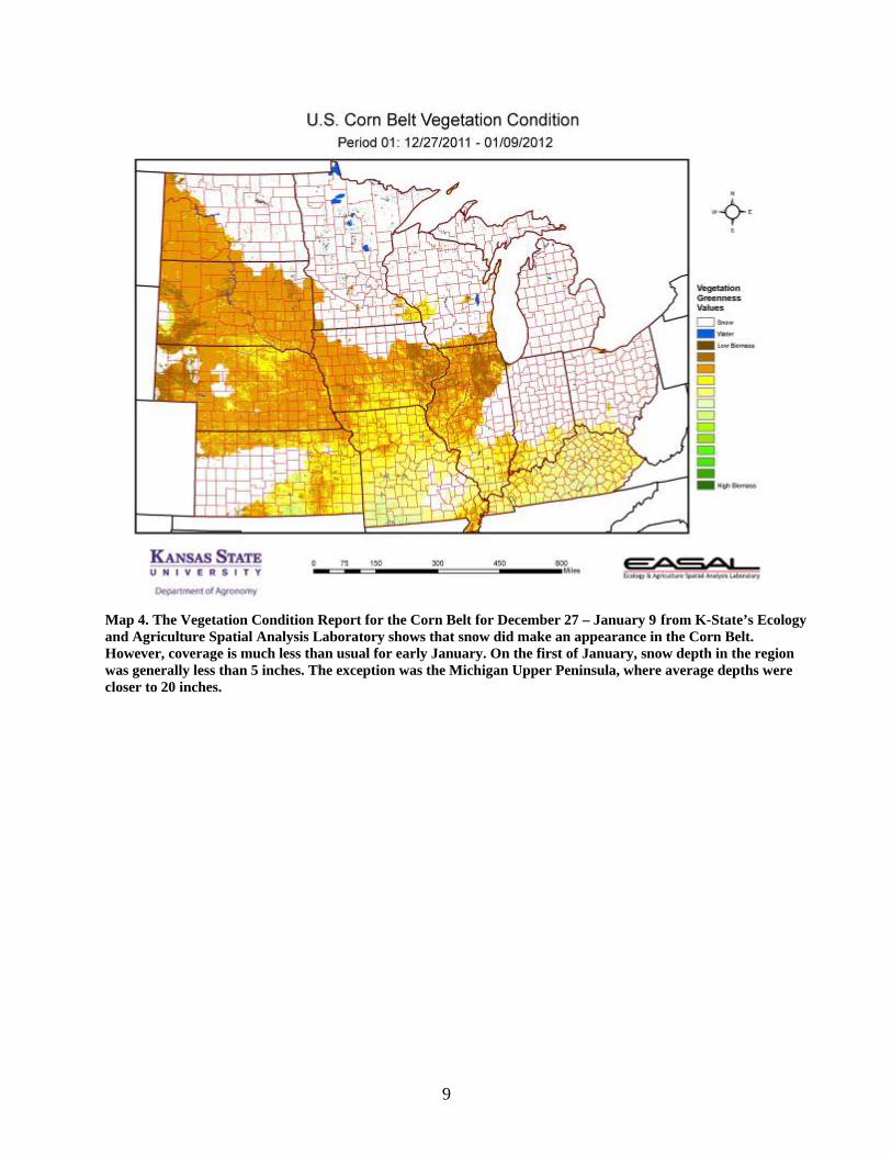
Map 4. The Vegetation Condition Report for the Corn Belt for December 27 – January 9 from K-State’s Ecology and Agriculture Spatial Analysis Laboratory shows that snow did make an appearance in the Corn Belt. However, coverage is much less than usual for early January. On the first of January, snow depth in the region was generally less than 5 inches. The exception was the Michigan Upper Peninsula, where average depths were closer to 20 inches.

10

Map 5. The comparison to last year in the Corn Belt for the period December 27 – January 9 from K-State’s Ecology and Agriculture Spatial Analysis Laboratory shows the impact of snow cover on photosynthetic activity. The much greater level of photosynthetic activity in the upper reaches of the Corn Belt is the result of more vegetation being visible than at this time last year.

11

Map 6. Compared to the 22-year average at this time for the Corn Belt, this year’s Vegetation Condition Report for December 27 – January 9 from K-State’s Ecology and Agriculture Spatial Analysis Laboratory shows that photosynthetic activity is greater than average across the region. The northern parts of Wisconsin and Upper Michigan have closer to normal levels of photosynthetic activity. These areas have closer-to-normal snow packs. In southwest Kansas, lingering snow cover from the late December storms also reduced photosynthetic activity.

12

Map 7. The Vegetation Condition Report for the U.S. for December 27 – January 9 from K-State’s Ecology and Agriculture Spatial Analysis Laboratory shows that the most notable feature is the snow cover in the Southwest, particularly New Mexico and the Texas Panhandle. The Midland, Texas preliminary report has it as the snowiest December on record. In contrast, Montana has had little snow cover.

13

Map 8. The U.S. comparison to last year at this time for the period December 27 – January 9 from K-State’s Ecology and Agriculture Spatial Analysis Laboratory shows decreased photosynthetic activity in southern Colorado and northern New Mexico. This corresponds with the region of above normal snowfall.

14

Map 9. The U.S. comparison to the 22-year average for the period December 27 – January 9 from K-State’s Ecology and Agriculture Spatial Analysis Laboratory shows lower-than-average photosynthetic activity in southeastern Colorado into western Kansas. This is due to a combination of lingering drought conditions and heavy snow cover. In western Pennsylvania, the lower-than-average level of photosynthetic activity is more difficult to explain. There are no drought conditions reported in the area, and most vegetation would be dormant at this time. Note to readers: The maps above represent a subset of the maps available from the EASAL group. If you’d like digital copies of the entire map series please contact us at kpprice@ksu.edu and we can place you on our email list to receive the entire dataset each week as they are produced. The maps are normally first available on Wednesday of each week, unless there is a delay in the posting of the data by EROS Data Center where we obtain the raw data used to make the maps. These maps are provided for free as a service of the Department of Agronomy and K-State Research and Extension. -- Mary Knapp, State Climatologist mknapp@ksu.edu -- Kevin Price, Agronomy and Geography, Remote Sensing, Natural Resources, GIS kpprice@ksu.edu -- Nan An, Graduate Research Assistant, Ecology & Agriculture Spatial Analysis Laboratory (EASAL) nanan@ksu.edu

These e-Updates are a regular weekly item from K-State Extension Agronomy and Steve Watson, Agronomy e-Update Editor. All of the Research and Extension faculty in Agronomy will be involved as sources from time to time. If you have any questions or suggestions for topics you'd like to have us address in this weekly update, contact Steve Watson, 785-532-7105 swatson@ksu.edu, or Jim Shroyer, Research and Extension Crop Production Specialist and State Extension Agronomy Leader 785-532-0397 jshroyer@ksu.edu