1 Density functions, cummulative density func-

tions, measures of central tendency, and mea-sures of dispersion

densityfunctions-intro.tex October 1, 2009

Note that this section of notes is limitied to the consideration ofa single and continuous random variable.

Remember from earlier that the variable X is a one-dimensional, continuousrandom variable if there exists a function f(x) such that f(x) � 0 8 x in theinterval �1 � x � 1, and the probability that (a � x � b) is

Pr(a � x � b) =bZa

f(x)dx

The function f(x) is called a density function (or a probability density func-tion).

1

1.1 Examples of density functions

the normal:

f(x) =1p2��

e�(x�u)2=2�2

is a well known density function where � and u are parameters in the densityfunction.

Who �rst expressed this formula? Who �rst used it as a density function?

2

Graphs of the normal probability density functions are the familiar bell-shaped curves. The following plots show the probabilitydensity functionsNormalDen (x;�; �),cumulative distribution functionsNormalDist (x;�; �) for the parameters (�; �) =(0; 1) ; (0; 5) ; (0; 0:5) ; (1; 1).

0

0.2

0.4

0.6

0.8

­4 ­2 2 4x

Normal density functions

0

0.2

0.4

0.6

0.8

1

­4 ­2 2 4x

Normal distribution functions

But, be warned that

tZ�1

1p2��e�(t�u)

2=2�2dt does not have a closed-form so-

lution.1

Lets start more simply.

1Note thatp2�� =

p2��2, ones sees the density function written both ways, and the

distinction is easy to miss.

3

1.1.1 Consider the Following Four Density Functions

Example 1 Assumeg(x) = 0 if x < 0 or x > 3

and

g(x) = 3x; 0 � x � 33Z0

3xdx = 1:5x2j30 = 1:5(9) = 13:5 6= 1

So, g(x) is not a density function, but

f(x) =3x

13:5

is.

That isf(x) = 0 if x < 0 or x > 3

andf(x) = :222x if 0 � x � 3

4

Note the importance of being explicit about where f(x) = 0.

Example 2

f(x) =

�1

18

�(3 + 2x) 2 � x � 4

f(x) = 0 otherwise

Is this a density function?f(x) � 0 8 x

Integrate it to see if the area under it is one.

1Z�1

f(x)dx =

2Z�1

0dx+

4Z2

�1

18

�(3 + 2x) dx+

1Z4

0dx

=1

18

4Z2

(3 + 2x) dx =1

18

�3x+ x2

�j42 =

1

18[(12 + 16)� (6 + 4)]

= 1

So, yes.

5

Example 3

f(x) = se�s(x�n) exph�e�s(x�n)

is > 0

The parameters are s and n.

Use Mathematica to graph this function and see show it changes as s and nchange.

f(x) � 0 8 xZf(x)dx =

Zse�s(x�n) exp

h�e�s(x�n)

idx

= exph�e�s(x�n)

iWhy? Recollect that Z

m0(x)em(x)dx = em(x)

So

1Z�1

f(x)dx = limb!+1

exph�e�s(b�n)

i� lima!�1

exph�e�s(a�n)

i= 1 + 0 = 1

Sof(x) = se�s(x�n) exp

h�e�s(x�n)

iis a density function. It is called the Extreme Value Distribution. It is the

foundation of logit models of choice.

6

Here are three examples of the Extreme Value Distribution. All have n = 0,the blue is s = 2, the red is s = :5 and the black is s = 1.

52.50­2.5­5

0.625

0.5

0.375

0.25

0.1250

x

y

x

y

Here are three more examples. All have s = 2, the red is n = �1, the blueis n = 3 and the black is n = 1.

52.50­2.5­5

0.625

0.5

0.375

0.25

0.1250

x

y

x

y

7

Example 4

f(x) =

�1

�

�1

1 + (x� u)2�1 < x <1

f(x) � 0 8 x1Z�1

f(x)dx =

�1

�

� 1Z�1

1

1 + (x� u)2dx

=

�1

�

�limb!1

arctan (b� u)��1

�

�lim

a!�1arctan (a� u)

Note arctan ( )= tan�1( ).

1Z�1

f(x)dx =

�1

�

���2

���1

�

����2

�=1

2+1

2= 1

f(x) =�1�

�1

1+(x�u)2 is called the Cauchy distribution.2

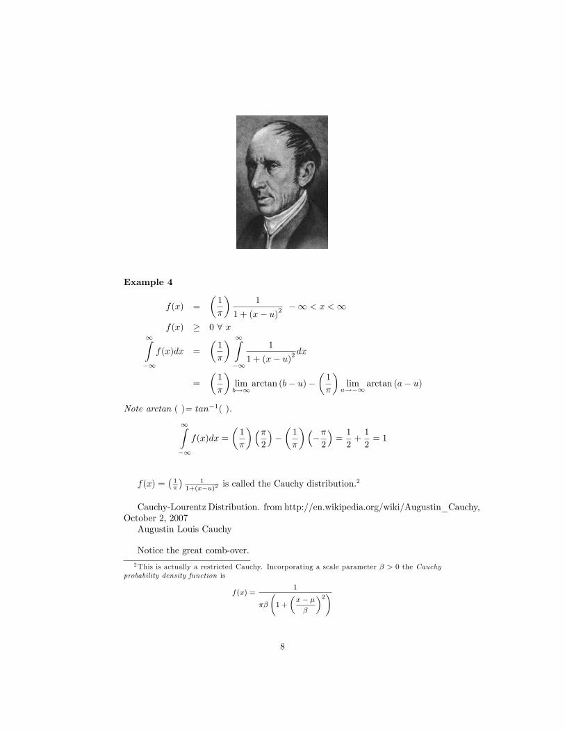
Cauchy-Lourentz Distribution. from http://en.wikipedia.org/wiki/Augustin_Cauchy,October 2, 2007Augustin Louis Cauchy

Notice the great comb-over.

2This is actually a restricted Cauchy. Incorporating a scale parameter � > 0 the Cauchyprobability density function is

f(x) =1

��

1 +

�x� ��

�2!

8

Born 21 August 1789, Dijon, FranceDied, 23 May 1857 (aged 67)Now you might ask who Lourentz is, http://en.wikipedia.org/wiki/Hendrik_Lorentz,

October 2, 2007Hendrik Antoon LorentzBorn July 18, 1853, Arnhem, NetherlandsDied February 4, 1928 (aged 74)Nobel Prize for Physics (1902)

The median of this distribution is �. The Cauchy probability density func-tion is symmetric about � and has a unique maximum at u.

If u = 0 it simpli�es to the Willy/Marshall distribution. (Willy and Marshalwere two former students.)

f(x) =

�1

�

�1

1 + x2

The Cauchy distribution is kind of cool: it does not have a mean or avariance.3

1.2

3Or, for that matter, any moments. We have yet to talk about moments.

9

1.3 Given the density function, f(x),

1.4

1.5

Pr(a � x � b) =bZa

f(x)dx

.For example 1

f(x) = 0:222x 0 � x � 3= 0 otherwise

so

Pr(1 � x � 2) =2Z1

(0:222x) dx = 0:111x2j21

= 0:111 [4� 1] = 0:333 = 1

3

For example 2

f(x) =

�1

18

�(3 + 2x) 2 � x � 4

= 0 otherwise

so

Pr(2 < x < 3) = Pr ob(2 � x � 3) =3Z2

f(x)dx

=1

18

3Z2

(3 + 2x) dx =1

18

�3x+ 2x2

�j32

=1

18[(9 + 9)� (6 + 4)]

=1

188 =

8

18

10

For example 3

f(x) = se�s(x�n) exph�e�s(x�n)

is > 0

so

Pr (�1 < x < b) = Pr (x � b)

=

bZ�1

f(x)dx =

bZ�1

se�s(x�n) exph�e�s(x�n)

idx

= exph�e�s(b�n)

i� lima!�1

exph�e�s(a�n)

ibut

lima!�1

exph�e�s(a�n)

i= 0

because as a! �1;�s (a� n)!1

Therefore, as a! �1;e�s(a�n) !1

So, as a! �1;�e�s(a�n) ! �1

andexp

h�e�s(a�n)

i! 0

Therefore, for the Extreme Value Distribution

Pr(x � b) = exph�e�s(b�n)

i

11

For example,

Pr(x � n) = exph�e�s(n�n)

i= exp

��e0

�= exp [�1] = e�1 = 1

e

Consider n+ :3665s (where did this come from?) What is the probability that

x � n+ :3665s ?

Pr ob

�x � n+ :3665

s

�= exp

h�e�s(n+ :3665

s �n)i

= exph�e�s( :3665s )

i= exp

��e�:3665

�= :5

What is n+ :3665s ? It is the median of the EV distribution. How did I �gure

out that this is the median of the EV distribution? Since

Pr(x � b) = exph�e�s(b�n)

iat median

Pr(x � median) = exph�e�s(median�n)

i= :5

by de�nition of the median. Simplify by letting � = s (median� n)

! exp��e��

�= 0:5

Solve for � by taking the ln of each side

! � = :366512921

but � = s (median� n) : Solve for

median = n+:366512921

s

12

For example 4

f(x) =

�1�

�(1 + x2)

u = 0

so

Pr(x > 0) =

1Z0

f(x)dx =

�1

�

� 1Z0

1

1 + x2dx

=

�1

�

��limb!1

arctan b

���1

�

�[arctan 0]

=

�1

�

���2

���1

�

�0

=1

2� 0 = 1

2

In words, zero is the median of the Willy/Marshall distribution.

1.6

13

1.7 Given the density function f(x), what is the proba-bility that X is less than or equal to x, where x is aspeci�c value of X?

Denote this probability

Pr(X � x) = F (x) �1 < x <1

where

Pr(X � x) = F (x) =xZ�1

f(t)dt

So the probability that x � b is

Pr(X � b) = F (b) =bZ

�1

f(t)dt =

bZ�1

f(x)dx

F (x) is called the cumulative density function for x.

We have already calculated the CDF (cumulative density function) for theExtreme Value Distribution and determined that

F (x) = exph�e�s(x�n)

i

14

What is the CDF for?For Example 1

f(x) = 0:222x 0 � x � 3= 0 otherwise

so

F (x) =

xZ�1

f(t)dt

F (x) = 0 if x � 0

F (x) =

xZ0

0:222t dt = :111t2jx0 = :111x2 if 0 < x < 3

F (x) = 1 if x � 3

15

For Example 2

f(x) =

�1

18

�(3 + 2x) 2 � x � 4

= 0 otherwise

so

F (x) = 0 if x < 2

F (x) = 1 if x � 4

F (x) =

xZ2

�1

18

�(3 + 2t) dt =

�1

18

��3t+ 2t2

�jx2

=

�1

18

���3x+ 2x2

�� (6 + 4)

�=

�1

18

��3x+ 2x2 � 10

�if 2 � x � 4

16

For Example 3

We have already determined that for the Extreme Value Distribution

F (x) = exph�e�s(x�n)

i

17

For Example 4Trig

Looking it up: The CDF for the Cauchy is

F (x) =1

�arctan(

x� ��

) +1

2

18

For the normal distribution

There is also no closed-form solution for F (x) for the normal distribution.That is

xZ�1

f(t)dt

does not have a closed-form solution if

f(x) =1p2��

e�(x�u)2=2�2

However, given speci�c values for u and �2, one can numerically solvexR�1f(t)dt for any x. Most statistics books provide tables for x given u = 0

and �2 = 1(the standard normal). Now there are web sites that provide thesetables interactively, you plug in u; �2 and x and out comes the probability thatX � x.

1.8

19

1.9 Note that if

F (a) = Pr(x < a)

then1� F (a) = Pr(x > a)

becauseF (a) + (1� F (a)) = 1

20

1.10 Measures of central tendency

Measures of central tendency are ways to describe one aspect of a distribution,f(x). Three measures of central tendency are:

� mean (expected value)

� median

� mode

The mean (expected value) of any continuous random variable x with dis-tribution f(x) is de�ned as

E(X) =

1Z�1

xf(x)dx

.What does E(X) mean (no pun intended)? If one randomly sampled one

X, one would not expect it to be E(X), so it is not the number you "expect."But, if one randomly sampled N X�s, one would expect the average value ofthe sampled x�s to ! E(X) as N !1.

The median of a continuous random variable x with density function f(x)is de�ned as u where

uZ�1

f(x)dx =1

2=

1Zu

f(x)dx

Given my de�nition of the median, Is the median always a unique number,or can it be a range? Should we change my de�nition so that it only exists when� is unique?If a density function has a unique global max, the value of x that max f(x) is

called the mode. Very loosely speaking, the mode is the most common value forx (remember that if x is continuously distributed the probability of observingany speci�c value of x is zero).

If the distribution is symmetric, mean = median.

For some distributions, mean = median = mode: e.g. the normal and thelogistic.

Not that some distributions do not have a mean.

21

The mean of (example 1)

f(x) = 0:222x 0 � x � 3= 0 otherwise

so

E(X) =

1Z�1

xf(x)dx =

0Z�1

xf(x)dx+

3Z0

xf(x)dx+

1Z3

xf(x)dx

=

0Z�1

x0dx+

3Z0

x (:222)xdx+

1Z3

x0dx

= 0 +

3Z0

(:222)x2dx+ 0 =:222

3x3j30 = 0:74x3j30

= 2

The mean of (example 2)

f(x) =

�1

18

�(3 + 2x) 2 � x � 4

= 0 otherwise

is

E(X) =

1Z�1

xf(x)dx =

2Z�1

xf(x)dx+

4Z2

xf(x)dx+

1Z4

xf(x)dx

=

2Z�1

x0dx+

4Z2

x

�1

18

�(3 + 2x) dx+

1Z4

x0dx

= 0 +

�1

18

� 4Z2

�3x+ 2x2

�dx+ 0

=

�1

18

��3

2x2 +

2

3x3�j42 =

�1

18

��3

2(16) +

2

3(64)�

�3

2(4) +

2

3(8)

��=

1

18[(24 + 42:666)� (6 + 5:333)] = 1

18[66:666� 11:333]

= 3:074

22

For the Extreme Value Distribution (example 3)

f(x) = se�s(x�n) exph�e�s(x�n)

iso

E(X) =

1Z�1

xf(x)dx =

1Z�1

xse�s(x�n) exph�e�s(x�n)

idx

=

1Z�1

xm0(x)em(x)dx =?

wherem(x) = �e�s(x�n)

I know that E(X) = n+ s where is the Euler constant (0:577). But I have

been unable to derive it analytically. Can you?

23

Can you do it for a speci�c values of n and s? For example, if n = 0 ands = 1,

E(X) =

1Z�1

xf(x)dx =

1Z�1

xe�(x) exph�e�(x)

idx

Given E(X) = n + s , if s = 1 and n = 0, E(X) = n +

s = = 0:577::::

Looking at the graph of e�(x) exp��e�(x)

�, one might guesstimate that E(X) =

0:577:::, is a bit greater than zero.

2.51.250­1.25­2.5

0.35

0.3

0.25

0.2

0.15

0.1

0.050

x

y

x

y

24

In this special case (n = 0 and s = 1), E(X) =1R�1xf(x)dx =

1Z�1

xe�x exp [�e�x] dx ,

my math software can �gure out the correct answer. Note that below I am tak-ing the de�nite integral over an every increasing range, and that the answer isapproaching . (My software will get mad if I plug in positive and negativein�nity)R 1

�1 xe�x exp [�e�x] dx = 1: 750 5� 10�2

R 2�2 xe

�x exp [�e�x] dx = 0:194 48R 5�5 xe

�x exp [�e�x] dx = 0:536 91R 10�10 xe

�x exp [�e�x] dx = 0:576 72R 20�20 xe

�x exp [�e�x] dx = 0:577 22

If I wanted to generalize I would continue to assume s = 1 and try to takethe de�nitie integral for di¤erent values of n to see how this a¤ects the answer.Hopefully, I would �nd that E(X) = n + , and, then if that works, I wouldstart playing with di¤erent values for s.

As an aside, note that the mode is n.

25

For the Cauchy Distribution (example 4)It does not have a mean. Wow. For a bit of explanation as to why, see the

asides at the end of this lecture.

26

1.10.1 Medians

We have already determined the median for the Extreme Value Distribution(example 3) and the Willy/Marshall distribution (example 4).

If u is the medianPr(x � u) = :5

For the Extreme Value Distribution

f(x) = se�s(x�n) exph�e�s(x�n)

iEarlier we determined that

median = n+ :3665

s

Recollect thatmean = E(X) = n+

s

where is the Euler constant ~:577216:

So, mean 6= median and

mean�median =�n+

:577216

s

���n+ :

3665

s

�=:21070

s

27

Earlier we determined that the median for the Willy/Marshall distribution is0. More generally the median of the Cauchy distribution is � - it has a median,just not a mean.

Determine the mode for the four example distributions?

28

1.11 Measures of dispersion

One question we often ask about distributions is: How dispersed or spread outare the values of X?

The most common measure of spread is variance. The variance is a measureof dispersion around the mean (E(X)).

V ariance � �2 � Eh(x� E(X))2

i� expected value of (x� E(X))2

Another possible measure of the dispersion around the mean is

E [jx� E(X)j]

.

One could alternatively de�ne measures of dispersion around the median ormode.

29

It can be shown that if f(x) is the density function for x and g(x) is somefunction of x

E [g(x)] =

1Z�1

g(x)f(x)dx

(this is a formula we will use often.)4 We used a special case of this formulato get E(X) = mean. That is, if g(x) = x

E [X] =

1Z�1

xf(x)dx

We can also use it to get

�2 � Eh(x� E(X))2

iIn this case, g(x) = (x� E(X))2 and

�2 � Eh(x� E(X))2

i=

1Z�1

(x� E(X))2 f(x)dx

4 Investigate why it is true.

30

Let�s calculate the variance of x for our earlier examples.For example 1

f(x) = 0:222x 0 � x � 3= 0 otherwise

The variance is

�2 =

1Z�1

(x� E(X))2 f(x)dx

Since E(X) = 2,

�2 =

1Z�1

(x� 2)2 f(x)dx

=

0Z�1

(x� 2)2 0dx+3Z0

(x� 2)2 (:222x) dx+1Z3

(x� 2)2 0dx

=

3Z0

(x� 2)2 (:222x) dx

= :5

31

So, what does this mean? In words, what does a variance of :5 mean?For example 2

f(x) =

�1

18

�(3 + 2x) 2 � x � 4

= 0 otherwise

Since E(X) = 3:074, the variance of x is

�2 =

1Z�1

(x� E(X))2 f(x)dx

=

1Z�1

(x� 3:074)2 f(x)dx

=

2Z�1

(x� 3:074)2 0dx4

+

Z2

(x� 3:074)2�1

18

�(3 + 2x) dx+

1Z4

(x� 3:074)2 0dx

=

4Z2

(x� 3:074)2�1

18

�(3 + 2x) dx

= :327846

32

For Example 3

Can we �gure out the variance for the Extreme Value Distribution?

f(x) = se�s(x�n) exph�e�s(x�n)

iSince E(X) = n+

s , where is Euler�s constant

�2 =

1Z�1

(x� E(X))2 se�s(x�n) exph�e�s(x�n)

idx

=

1Z�1

�x� (n+

s)�2se�s(x�n) exp

h�e�s(x�n)

idx

Luckily for us, someone (?) has already determined that

�2 =�2

6s2

33

Example 4 (the Cauchy distribution). Since it does not have an E[X], itcannot have a well-de�ned variance because the variance is a function of theE[X].

For the normal density function

f(x) =1p2��

e�(x�u)2=2�2

the variance is simply �2.

34

1.12 Some asides

1.12.1 Is there a way to derive the E[X] directly from the CDF?

The answer is yes (from MGB), as there must be:

E[X] =

+1Z0

[1� F (x)] dx�0Z�1

F (x)dx

Can you intuite this? Try it out and see if it works. If I remember cor-rectly, this formula is useful if the one has a mixed distribution (discrete andcontinuous).

Maybe, you could use it to get E[X] for the Extreme Value distribution,

where F (x) = exp��e�s(x�n)

�, E[X] =

+1Z0

[1� F (x)] dx�0Z�1

F (x)dx =

+1Z0

�1� exp

��e�s(x�n)

��dx�

0Z�1

exp��e�s(x�n)

�dx. NOPE

35

1.12.2 Some probabilities of interest

For some distributions, one you determine Pr[(E[X] � �) � x � (E[X] + �)]where � is de�ned as the variance, or Pr[(E[X]� 2�) � x � (E[X] + 2�)]. The�rst is the probability that a randomly drawn X lies between (E[X] � �) and(E[X] + �)

For a given f (x) ; this is the probability that ........?

At this point, you should have the tools to �gure these out? Will the valueof Pr[(E[X] � �) � x � (E[X] + �)] be a function of f(x)? or be invariant tothe form of the density function?

For example, in terms of the CDF, F (X)

Pr[(E[X]� �) � x � (E[X] + �)]= F (E[X] + �)� F ((E[X]� �))

36

It looks like it is a function of F (X), so not invariant to the form of thedistribution.5

1.12.3 E[X] and variance as areas

Recollect that if f(x) is a density function then

+1Z�1

f(x)dx = 1, where

+1Z�1

f(x)dx

is the area under the density function.

E(X) =1R�1xf(x)dx can be thought of as an area, the area under the func-

tion xf(x).

And, variance is the area under (x� E[X])2f(x). That is, mean and variancecan be viewed as areas.

So the mean will not be well de�ned unless the area under xf(x) is wellde�ned, and the variance will not be well de�ned unless the area under (x �E[X])2f(x) is well de�ned - this will sometimes be an issue, mostly with densityfunctions where f(x) > 0 �1 < x < +1.

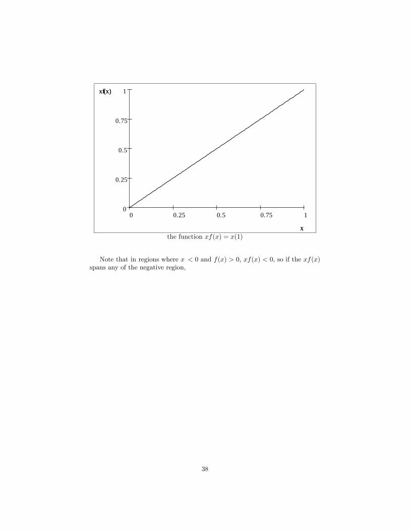
Consider the uniform distribution on the unit interval, a very simple exam-ple. For this density, xf(x) is a straight line from (0; 0) to (1; 1) , and the areaunder it is :5 = E[X]

5Many students tend to think, incorrectly, that Pr[(E[X]��) � x � (E[X]+�)] is invariantto the form of F (X)

37

10.750.50.250

1

0.75

0.5

0.25

0

x

xf(x)

x

xf(x)

the function xf(x) = x(1)

Note that in regions where x < 0 and f(x) > 0, xf(x) < 0, so if the xf(x)spans any of the negative region,

38

it will have negative area in those sections.

39

Consider, for example, the uniform distribution on the interval (�:5;+:5).For this density function, xf(x) is a straight line from (�:5;�:5) to (:5; :5); thearea under it to the left of zero is �:25 and to the right of zero is +:25 andE[X] = 0.

0.50.250­0.25­0.5

0.5

0.25

0

­0.25

­0.5

x

xf(x)=x

x

xf(x)=x

:5Z�:5

xdx = 0:0

40

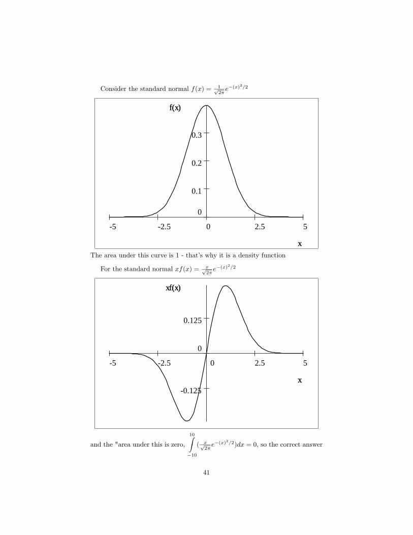
Consider the standard normal f(x) = 1p2�e�(x)

2=2

52.50­2.5­5

0.3

0.2

0.1

0

x

f(x)

x

f(x)

The area under this curve is 1 - that�s why it is a density function

For the standard normal xf(x) = xp2�e�(x)

2=2

52.50­2.5­5

0.125

0

­0.125x

xf(x)

x

xf(x)

and the "area under this is zero,

10Z�10

( xp2�e�(x)

2=2)dx = 0, so the correct answer

41

for the mean of the standard normal.

How about the variance (which we know is 1). It is the area under (x �0)2f(x) = x2p

2�e�(x)

2=2

52.50­2.5­5

0.25

0.2

0.15

0.1

0.050

x

y

x

y

Z 5

�5( x2p

2�e�(x)

2=2)dx = 0:999 98, wow, the correct answer.

Further note that we can always write

E(X) =

1Z�1

xf(x)dx

=

0Z�1

xf(x)dx+

+1Z0

xf(x)dx

=

+1Z0

xf(x)dx�0Z�1

jxj f(x)dx

42

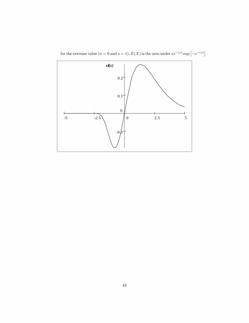
for the extreme value (n = 0 and s = 1), E(X) is the area under xe�(x) exp��e�(x)

�

52.50­2.5­5

0.2

0.1

0

­0.1

xf(x)xf(x)

43

As from beforeR 25�25 xe

�x exp [�e�x] dx = 0:577 22

1.12.4 Density functions where f(x) > 0 �1 < x < +1

1.12.5

The normal, the Cauchy and the Extreme Value are all density function whereevery value of X has positive density.

Imagine you are trying to create a new density function where f(x) > 08x. The area under many functions that meet the condition f(x) > 0 8x have+1Z�1

f(x)dx = +1, so cannot be density functions.

One must choose carefully: one must choose a function so that as one in-tegrates over larger and larger ranges of X, the area under the function mustforever increase, but at the same time the area can never be greater than one -neat trick.

The normal, the Cauchy and the Extreme value, since they all are densityfunctions, do the trick. But the fact that the area under f(x) is well de�ned, does

not imply that the areas under xf(x) and (x� E[X])2f(x) are well de�ned.6

These areas are well de�ned for the normal and the Extreme value, but theyare not for the Cauchy - that is why the Cauchy does not have a mean.

Put loosly, the reason the Cauchy does not have a mean is that

0Z�1

xf(x)dx =

�1 and

+1Z0

xf(x)dx = +1 - the tails of xf(x) are too fat.

6Note that if the area under xf(x) is not well de�ned, then (x� E[X])2f(x) is not wellde�ned.

44

The following is from Wikipedia.

Go �gure!

45