1 changes to ac-4 - algorithm ac-6 –algorithm ac-6 avoids the outlined inefficiency of ac-4 with a...

1

• Changes to AC-4 - Algorithm AC-6

– Algorithm AC-6 avoids the outlined inefficiency of AC-4 with a basic idea: instead of keeping (counting) all values vi from variable Xi that support a pair Xj-vj, it simply maintains the lowest such vi that supports the pair.

– The initialisation of the algorithm becomes “lighter”, since whenever the first value vi is found, no more supporting values are seeked and no counting is required.

– AC-6 also does not require the initialisation of supporting sets, i.e. to keep the set of all pairs Xi-vi supported by a pair Xj-vj, but only the lowest such supported vi.

– Of course, if these values are not initialised, they must be determined during the propagation phase!

Maintaining Arc Consistency: AC-6

2


• Data Structures of Algorithm AC-6

– The List and the Boolean matrix M from AC-4 are kept.

– The AC-4 counters are disposed of;

– The supporting sets become “singletons”, keeping only the lowest value supported (it is assumed that some ordering is defined for the domains)

sup(2,X1) = [X2-4,X3-1,X3-3,X4-1,X4-3,X4-4]

% X1-2 supports(no attack) X2-4, X3-1,...

sup(1,X1) = [X2-2, X2-3 , X3-2, X3-4, X4-2, X4-3]

sup(3,X1) = [X2-1, X3-2 , X3-4, X4-1, X4-2, X4-4]

sup(4,X1) = [X2-1, X2-2 , X3-1, X3-3, X4-2, X4-3]

3

• Both phases of AC-6 use predicate

next_support(Xi,vi,Xj,vj, out v)

that succeeds if there is in the domain of Xj a “next” supporting value v, the lowest value, no less than some value, vj, such that Xj-v supports Xi-vi.

predicate next_support(Xi,vi,Xj,vj, out v): boolean; sup_s <- false; v <- vj; while not sup_s and v =< max(dom(Xj)) do if not satisfies({Xi-vi,Xj-v},Cij) then

v <- next(v,dom(Xj)) else sup_s <- true end if end while next_support <- sup_s;

end predicate.


4

• Algorithm AC-6 (Phase 1 - Inicialisation)

procedure inicialise_AC-6(V,D,C); List <- ; M <- 0; sup <- ; for Cij in C do

for vi in dom(Xi) do v = min(dom(Xj)) if next_support(Xi,vi,Xj,v,vj) then sup(vi,Xi)<- sup(vi,Xi) {Xj-vj} else dom(Xi) <- dom(Xi)\{vi}; M[Xi,vi] <- 0; List <- List {Xi-vi} end if end forend for

end procedure


5

Algorithm AC-6 (Phase 1 - Inicialisation)

procedure propagate_AC-6(V,D,C);while List do List <- List\{Xj-vj} % removes Xj-vj from List for Xi-vi in sup(vj,Xj) do

sup(vi,Xi) <- sup(vi,Xi) \ {Xj-vj} ; if M[Xi,vi] = 1 then if next_suport(Xi,vi,Xj,vj,v) then sup(v,Xj)<- sup(v,Xj) {Xi-vi}

else dom(Xi) <- dom(Xi)\{vi}; M[Xi,vi]

<- 0; List <- List {Xi-vi} end if end if end for

end whileend procedure


6


Space Complexity of AC-6

In total, algorithm AC-6 maintains

Supporting Sets: In the worst case, for each of the a constraints Cij,

each of the d pairs Xi-vi is supported by a single value vj form Xj

(and vice-versa). Thus, the space required by the supporting sets

is O(ad).

List: Includes at most 2a arcs

Matrix M: Maintains nd Booleans.

The space required by the supporting sets is dominant, so algorithm AC-

6 has a space complexity of

O(ad)

between those of AC-3 ( O(a) ) and AC-4 ( O(ad2) ).

7


Time Complexity of AC-6

In both phases of initialisation and propagation, AC-6 executes

next_support(Xi,vi,Xj,vj,v) in its inner cycle.

For each pair Xi-vi, variable Xj is checked at most d times.

For each arc corresponding to a constraint Cij, d pairs Xi-vi are

considered at most.

Since there are 2a arcs (2 per constraint Cij), the time complexity,

worst-case, in any phase of AC-6 is

O(ad2).

Like in AC-4, this is optimal assymptotically.

8


Typical complexity of AC-6

• The worst case time complexity that can be inferred from the algorithms do not give a precise idea of their average behaviour in typical situations.

• For such study, one usually tests the algorithms in a set of “benchmarks”, i.e. problems that are supposedly representative of everyday situations.

• For these algorithms, either the benchmarks are instances of well known problems (e.g. N queens), or one relies on randomly generated instances parameterised by

• their size (number of variables and cardinality of the domains) ; and

• their difficulty (density and tightness of the constraint network).

9


Typical Complexity of algorithms AC-3, AC-4 e AC-6 (N-queens)

0

2000

4000

6000

8000

10000

12000

14000

16000

4 5 6 7 8 9 10 11

# t

est

s an

d o

pera

tion

s

AC-3

AC-4

AC-6

# queens

10


Typical Complexity of algorithms AC-3, AC-4 e AC-6 (randomly generated problems)

n = 12 variables, d= 16 values, density = 50%

02000400060008000

10000120001400016000180002000022000

5 10 15 20

25

30

35

40

45

50

60

70

80

# t

ests

and

ope

rati

ons

AC-3

AC-4

AC-6

Tightness (%)

11


Pitfalls of AC-6 - Algorithm AC-7

Algorithm AC-6 (like AC-4 and AC-3) unnecessarily duplicates support

detection, as it does not take into account that support is bidirectional,

i.e.

Xi-vi supports Xj-vj iff Xj-vj supports Xi-vi

Algorithm AC-7 will use this property to infer support, rather than search

for support.

Other types of inference could be used (for example, if one knows the

semantics of the constraints, namely whether they are transitive), but

AC-7 simply exploits the bidirectionality of support, which is always valid.

12


Example:

Assuming that 2 countries may be coloured with 3 colours. The different

AC-x algorithms will perform the following operation to initialise arc-

consistency.

AC-38 tests

AC-68 tests

AC-75 tests

2 inferences

AC-418 tests

13


Data Structures of Algorithm AC-7

Algorithm AC-7 keeps, for each pair Xi-vi a supporting set CS(vi,Xi,Xj),

that is the set of values from the domain of Xj currently supported by

pair Xi-vi.

It also keeps, for each triple (vi,Xi,Xj), a value last(vi,Xi,Xj) that

represents the last value (in increasing order) from the domain of Xj

that was tested for support of pair Xi-vi.

For all variables, it is assumed that the domains have an ordering and,

for convenience, artificial values top and bottom are added,

respectively higher and lower that any “real” value of the domain.

14

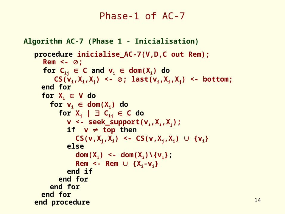
Phase-1 of AC-7

Algorithm AC-7 (Phase 1 - Inicialisation)

procedure inicialise_AC-7(V,D,C out Rem); Rem <- ; for Cij C and vi dom(Xi) do CS(vi,Xi,Xj) <- ; last(vi,Xi,Xj) <- bottom;end forfor Xi V do for vi dom(Xi) do for Xj | Cij C do v <- seek_support(vi,Xi,Xj); if v top then CS(v,Xj,Xi) <- CS(v,Xj,Xi) {vi} else dom(Xi) <- dom(Xi)\{vi}; Rem <- Rem {Xi-vi} end if end for end forend for

end procedure

15

Phase-2 of AC-7

Algorithm AC-7 (Phase 2 - Propagation)

procedure propagate_AC-7(V,D,C,Rem); while Rem do Rem <- Rem \ {Xj-vj} for Xi | Cij C do while CS(vj,Xj,Xi) do CS(vj,Xj,Xi) <- CS(vj,Xj,Xi) \ {vi} if vi dom(Xi) then v <- seek_support(vi,Xi,Xj); if v top then CS(v,Xj,Xi) <- CS(v,Xj,Xi) {vi}

else dom(Xi) <- dom(Xi)\{vi}; Rem <- Rem {Xi-vi} end if end if end while end for end while end procedure

16


Algorithm AC-7 (Auxiliary Function seek_support)

Function seek_support seeks, within the domain of Xj, some value vj that

supports pair Xi-vi. Firstly, it tries to infer such support in the pairs Xi-vi that

support Xj-vj (exploiting the bidireccionality of support). Otherwise, it

searches for vj in the domain of Xj in the usual way.

function seek_support(vi,Xi,Xj): value; if infer_support(vi,Xi,Xj,v) then seek_support <- v; else seek_support <- search_support(vi,Xi,Xj) end ifend function

Notice that functions search_support and seek_support may return the “artificial” value top.

17


Algorithm AC-7 (Auxiliary Predicate infer_support)

Exploiting the bidireccionality of support, the auxiliary predicate infer_support, looks for a value vj in the domain of variable Xj that supports pair Xi-vi.

predicate infer_support(vi,Xi,Xj,out vj): boolean; found <- false; while CS(vi,Xi,Xj) and not found do CS(vi,Xi,Xj) = {v} Z; if v in dom(Xj) then found <- true; vj <- v; else CS(vi,Xi,Xj) = CS(vi,Xi,Xj) \ {v}; end ifend doinfer_support <- found

end predicate.

18


Algorithm AC-7 (Auxiliary Function search_support)

function search_support(vi,Xi,Xj): value; b <- last(vi,Xi,Xj); if b = top then search_support <- b else found <- false; b <- next(b,dom(Xj)) while b top and not found do if last(b,Xj,Xi) =< vi and satisfies({Xi-vi,Xj-b}, Cij) then found <- true else b <- next(b,dom(Xj)) end if end while last(vi,Xi,Xj) <- b; search_support <- b; end if

end function;

19


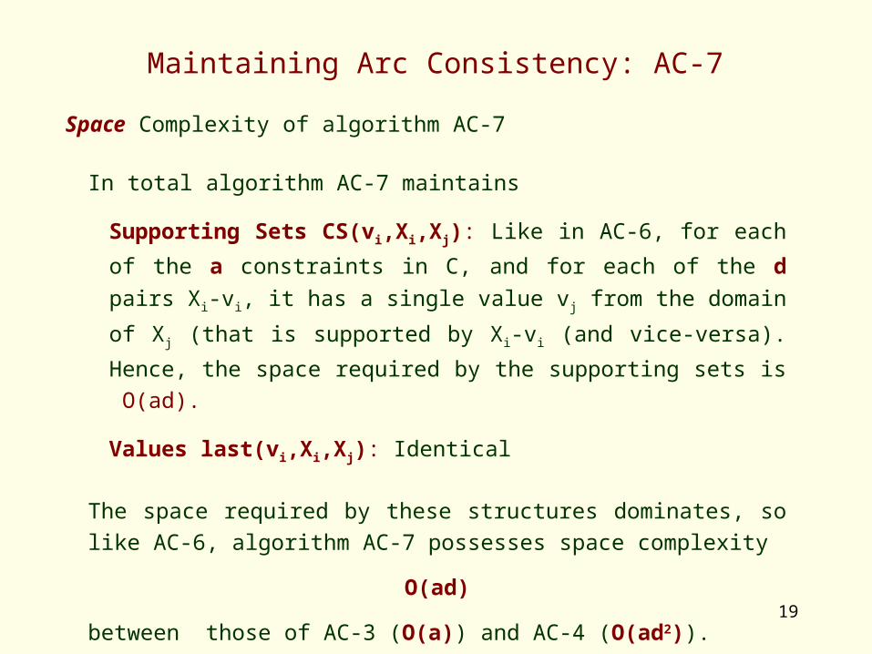
Space Complexity of algorithm AC-7

In total algorithm AC-7 maintains

Supporting Sets CS(vi,Xi,Xj): Like in AC-6, for each of the a

constraints in C, and for each of the d pairs Xi-vi, it has a single value

vj from the domain of Xj (that is supported by Xi-vi (and vice-versa).

Hence, the space required by the supporting sets is O(ad).

Values last(vi,Xi,Xj): Identical

The space required by these structures dominates, so like AC-6,

algorithm AC-7 possesses space complexity

O(ad)

between those of AC-3 (O(a)) and AC-4 (O(ad2)).

20


Time Complexity of algorithm AC-7

In both phases of initialisation and propagation, AC-7 executes

seek_support(vi,Xi,Xj) in its inner cycle.

There are at most 2ad triples (vi,Xi,Xj), since there are 2a arcs

corresponding to constraints in C, and the domain of each variable

has, at most, d values.

In each call to seek_support(vi,Xi,Xj), d values from the domain of

Xj, at most, are tested.

Hence, the worst-case time complexity of both phases of AC-7, is

similar to that of AC-6, namely

O(ad2).

which, as shown with AC-4, is assymptotically optimal.

21


Given their identical complexity, in what ways does AC-7 improve on AC-6 (and other AC-x algorithms)? Let us consider some features of AC-7.

1. It never tests Cij(vi,vj) if there is a v’j still in the domain of Xj such that

Cij(vi, v’j) was successfully tested.

2. It never tests Cij(vi,vj) if

a) It has already been tested; or

b) If Cij(vj,vi) was already tested.

3. It has space complexity O(ad)

In contrast, algorithm AC-3 only exhibits feature 3; AC-4 only feature 2a; and AC-6 exhibits features 1, 2a and 3, but not feature 2b.

22


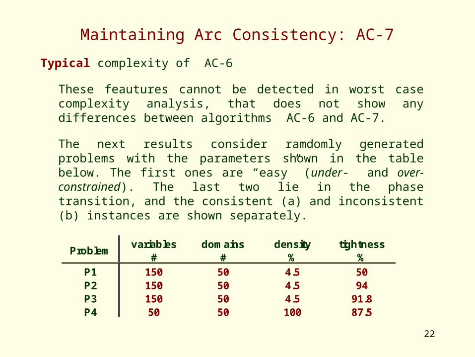
Typical complexity of AC-6

These feautures cannot be detected in worst case complexity analysis, that does not show any differences between algorithms AC-6 and AC-7.

The next results consider ramdomly generated problems with the parameters shown in the table below. The first ones are “easy” (under- and over-constrained). The last two lie in the phase transition, and the consistent (a) and inconsistent (b) instances are shown separately.

variables domains density tightness# # % %

P1 150 50 4.5 50P2 150 50 4.5 94P3 150 50 4.5 91.8P4 50 50 100 87.5

Problem

23


Comparison of Typical Complexity (# of checks)

0

1000000

2000000

3000000

4000000

5000000

6000000

7000000

8000000

9000000

Prob 1 Prob 2 Prob 3a Prob 3b Prob 4a Prob 4b

AC-3AC-4AC-6AC-7

24


Comparison of Typical Complexity

(CPU time, in ms, in a Pentium at 200 MHz)

0

1000

2000

3000

4000

5000

6000


AC-3AC-4AC-6AC-7

25

Maintaining Arc Consistency: AC-3d

Bidirectionality of support was also exploited in an adaptation, not of AC-6,

but rather of AC-3, resulting in algorithm A-3d.

The main difference between algorithms AC-3 and AC-3d consists of the

fact that whenever arc aij is removed from queue Q, the arc aji is also

removed, in case it is there.

In this case, both domains of Xi and Xj are revised, which avoids much

duplicated work.

Although it does not improve the worst-case complexity of AC-3, the

typical complexity of AC-3d seems quite interesting (namely in some

problems for which extensive tests were performed).

26



(previous ramdomly generated problems)

0

1000000

2000000

3000000

4000000

5000000

6000000

7000000

8000000

9000000


AC-3AC-4AC-6AC-7AC-3d

27



(previous ramdomly generated problems)

(equivalent CPU time, in ms, in a Pentium at 200 MHz)

0

1000

2000

3000

4000

5000

6000


AC-3AC-4AC-6AC-7AC-3d

28


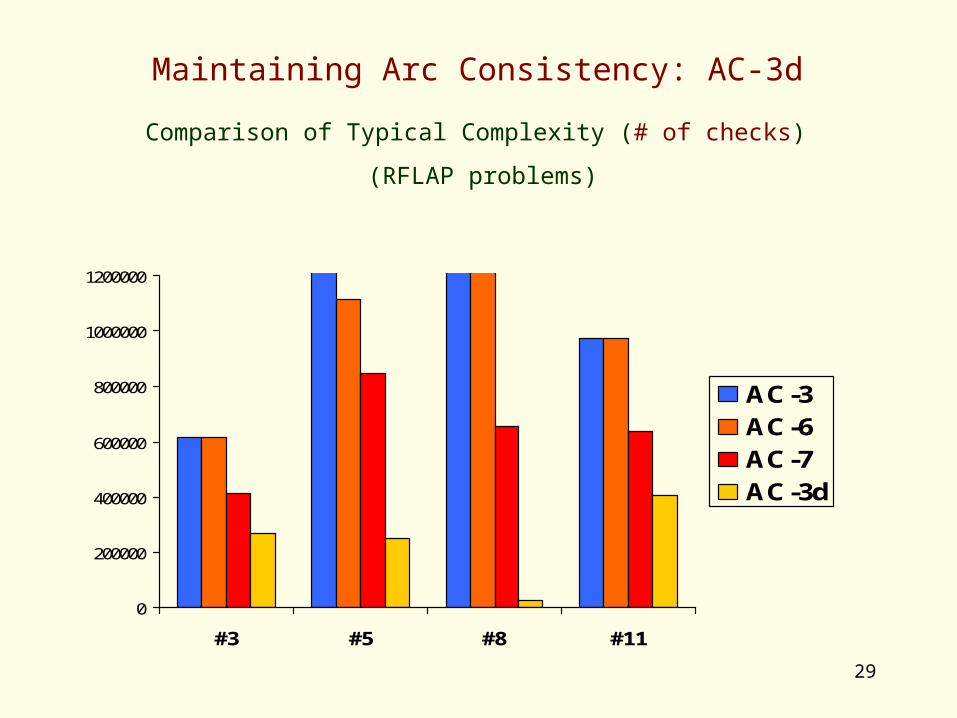
Results seem particularly interesting for problems in which AC-7 was

proved much superior to AC-6, both in number of tests and in CPU time.

This is the case of problem RLFAP (Radio Link Frequency

Assignment Problem), that consists of assigning radio frequencies in a

safe way (no risk of scrambling), for which instances with 3, 5, 8 e 11

antenae were studied.

The code ( as well as that of other benchmark problems) may be found

in a benchmark archive, available from the internet, in URL

http://ftp.cs.unh.edu/pub/csp/archive/code/benchmarks

29



(RFLAP problems)

0

200000

400000

600000

800000

1000000

1200000

#3 #5 #8 #11

AC-3AC-6AC-7AC-3d

30



(RFLAP problems)

(equivalent CPU time, in ms, in a Pentium at 200 MHz)

0

500

1000

1500

2000

2500

# 3 # 5 # 8 # 11

AC-3AC-6AC-7AC-3d

31

Path Consistency

In addition to arc consistency, other types of consistency may be defined

for binary constraint networks.

Path consistency is a “classical” type of consistency, stronger than arc

consistency.

The basic idea of path consistency is that, in addition to check support in

the arcs of the constraint network between variables Xi and Xj, further

support must be checked in the variables Xk1, Xk2... Xkm that form a path

between Xi and Xj, i.e. whenever there are constraints Ci,k1, Ck1,k2, ...,

Ckm-1, km and Ckm,j.

In fact, it is possible to show this is equivalent to seek support in any

variable Xk,connected to both Xi and Xj.

32

Path Consistency

Definition (Path Consistency):

A constraint satisfaction problem is path-consistent if,

1. It is arc-consistent; and

2. For every pair of variables Xi and Xj, and paths Xi–Xi1–Xi2 - ... -

Xin–Xj, the direct constraint Ci,j is tighter than the composition of

the constraints in the path Ci,i1, Ci1,i2, ... , Cin,j.

In practice, every value vi in variable Xi must have support, not only

in some value vj from variable Xj but also in values vi1, vi2 , ... , vin

from the domain of the vriables in the path.

33

Path Consistency

Maintaining this type of consistency has naturally a higher computational

cost than maintaining a simpler criterion such as arc consistency.

In order to do so, it is convenient to maintain a representation by

extension of the binary constraints, in the form of a boolean matrix.

Assuming that variables Xi and Xj have, respectively, di and dj values in

their domain, constraint Cij is maintained as a boolean matrix Mij of size

di*dj.

The value 1/0 of element Mij[k,l] indicates whether the pair {Xi-vk, Xj-vl}

satisfies/or not constraint Cij.

34

Path Consistency

Example: 4 queens

Boolean Matrix M12, regarding constraint C12 between variables X1 e X2 (or any variables in consecutive rows)

1\ 2 1 2 3 4

1 0 0 1 1

2 0 0 0 1

3 1 0 0 0

4 1 1 0 0

M12[1,3] = M12[3,1] = 1

1\ 3 1 2 3 4

1 0 1 0 1

2 1 0 1 0

3 0 1 0 1

4 1 0 1 0

Boolean Matrix M13, regarding constraint C12 between variables X1 and X2 (or any variables rows separed by one row)

M12[3,4] = M12[4,3] = 0

M13[1,2] = M13[2,1] = 1

M13[2,4] = M13[4,2] = 0

35

Path Consistency

Checking Path Consistency

To eliminate from matrix Mij (i.e. to zero an element) those values that do

not satisfy path consistency through a third variable, Xk, one may use

operations similar to matrix multiplication and sum.

MIJ <- MIJ MIK MKJ

where the operation operates like in a matrix “sum”, but with arithmetic

addition replaced by boolean conjunction, and the operation

corresponds to matrix multiplication in which arithmetic multiplication and

addition are replaced by boolean conjunction and disjunction.

One must still consider the diagonal matrix Mkk to represent the domain of

variable Xk.

36

Path Consistency

Example (4 queens):

Checking if compound label {X1-1 e X3-4} is path inconsistent, through

variable X2.M13[1,4] <- M13[1,4] M12[1,X] M23[X,4]

In fact, M12[1,X] M23[X,4] = 0 since

M12[1,1] M23[1,4] % X2- 1 does not support {X1-1,X3-4}

M12[1,2] M23[2,4] % X2-2 does not support {X1-1,X3-4}

M12[1,3] M23[3,4] % X2-3 does not support {X1-1,X3-4}

M12[1,4] M23[4,4] % X2-4 does not support {X1-1,X3-4}1\ 2 1 2 3 4 2\ 3 1 2 3 4 1\ 3 1 2 3 4 1\ 3 1 2 3 4

1 0 0 1 1 1 0 0 1 1 1 0 1 0 1 1 0 1 0 0

2 0 0 0 1 2 0 0 0 1 2 1 0 1 0 2 1 0 0 0

3 1 0 0 0 3 1 0 0 0 3 0 1 0 1 3 0 0 0 1

4 1 1 0 0 4 1 1 0 0 4 1 0 1 0 4 0 0 1 0

37

Path Consistency

Path consistency is stronger than arc consistency, in the sense that its

maintenace will allow, in general, to eliminate more redundant values from

the domains of the variables than simpler arc consistency is able to do

In particular, for the 4 queens problem, the maintenance of path

consistency performs the elimination from the domain of the variables of

all the redundant values, that do not belong to any solution, even before

any enumeration takes place!

The problem reduced by path consistency may thus be solved with a

backtracking-free enumeration.

Notice, that the enumeration and its backtracking is the cause of the

exponential complexity of solving non trivial problems.

38

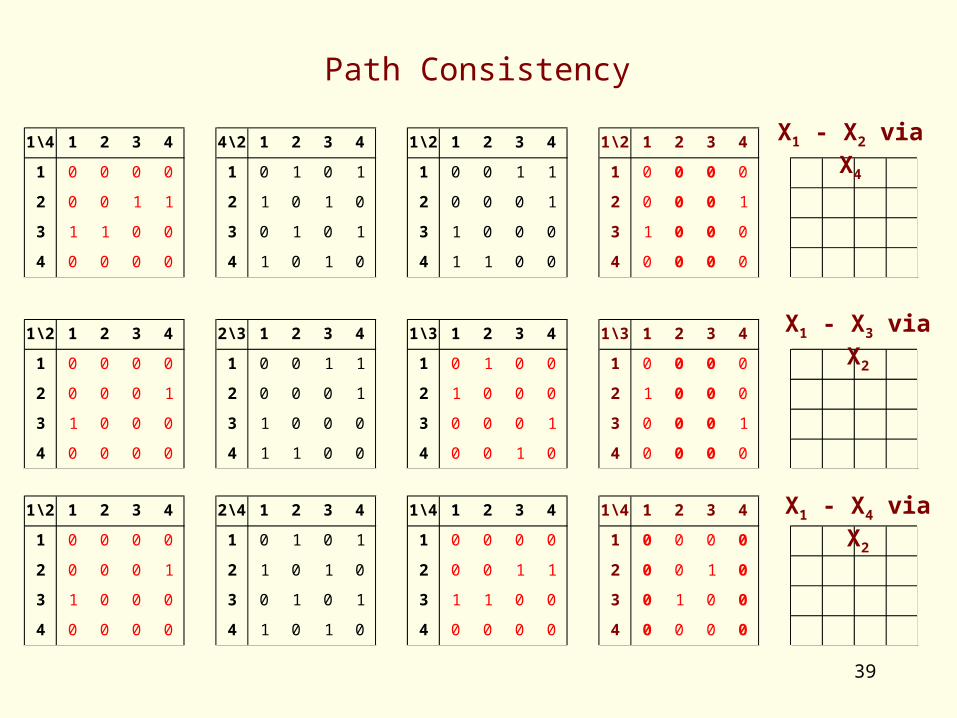
Path Consistency

Path consistency in the 4 queens problem

1\ 2 1 2 3 4 2\ 3 1 2 3 4 1\ 3 1 2 3 4 1\ 3 1 2 3 4

1 0 0 1 1 1 0 0 1 1 1 0 1 0 1 1 0 1 0 0

2 0 0 0 1 2 0 0 0 1 2 1 0 1 0 2 1 0 0 0

3 1 0 0 0 3 1 0 0 0 3 0 1 0 1 3 0 0 0 1

4 1 1 0 0 4 1 1 0 0 4 1 0 1 0 4 0 0 1 0

1\ 3 1 2 3 4 3\ 4 1 2 3 4 1\ 4 1 2 3 4 1\ 4 1 2 3 4

1 0 1 0 0 1 0 0 1 1 1 0 1 1 0 1 0 0 0 0

2 1 0 0 0 2 0 0 0 1 2 1 0 1 1 2 0 0 1 1

3 0 0 0 1 3 1 0 0 0 3 1 1 0 1 3 1 1 0 0

4 0 0 1 0 4 1 1 0 0 4 0 1 1 0 4 0 0 0 0

X1 - X3 via X2

X1 - X4 via X3

39

Path Consistency

1\ 4 1 2 3 4 4\ 2 1 2 3 4 1\ 2 1 2 3 4 1\ 2 1 2 3 4

1 0 0 0 0 1 0 1 0 1 1 0 0 1 1 1 0 0 0 0

2 0 0 1 1 2 1 0 1 0 2 0 0 0 1 2 0 0 0 1

3 1 1 0 0 3 0 1 0 1 3 1 0 0 0 3 1 0 0 0

4 0 0 0 0 4 1 0 1 0 4 1 1 0 0 4 0 0 0 0

1\ 2 1 2 3 4 2\ 3 1 2 3 4 1\ 3 1 2 3 4 1\ 3 1 2 3 4

1 0 0 0 0 1 0 0 1 1 1 0 1 0 0 1 0 0 0 0

2 0 0 0 1 2 0 0 0 1 2 1 0 0 0 2 1 0 0 0

3 1 0 0 0 3 1 0 0 0 3 0 0 0 1 3 0 0 0 1

4 0 0 0 0 4 1 1 0 0 4 0 0 1 0 4 0 0 0 0

1\ 2 1 2 3 4 2\ 4 1 2 3 4 1\ 4 1 2 3 4 1\ 4 1 2 3 4

1 0 0 0 0 1 0 1 0 1 1 0 0 0 0 1 0 0 0 0

2 0 0 0 1 2 1 0 1 0 2 0 0 1 1 2 0 0 1 0

3 1 0 0 0 3 0 1 0 1 3 1 1 0 0 3 0 1 0 0

4 0 0 0 0 4 1 0 1 0 4 0 0 0 0 4 0 0 0 0

X1 - X2 via X4

X1 - X3 via X2

X1 - X4 via X2

40

Path Consistency

Of course, this increase in the pruning power of path consistency does

not come for free. The computational complexity of achieving and

maintaining it is (much) greater than the costs associated with arc

consistency.

The algorithms to maintain path consistency, PC-x, have therefore

higher complexity than those of the AC-y family.

As an example, algorithm PC-1 (quite simple, with no optimisatiosn) is

presented.

The more sophisticated algorithms, PC-2 e PC-4, include optimisations

that avoid repetition of tests, much in the same way that the higher

members of the AC-y family do. We will simply outline the optimisations

and present their complexity.

41

Maintaining Path Consistency: PC-1

Algorithm PC-1

procedure PC-1(V,D,C); n <- #Z; Mn <- C; repeat M0 <- Mn; for k from 1 to n do for i from 1 to n do for j from 1 to n do Mij

k <- Mijk-1 Mik

k-1 Mkkk-1 Mkj

k-1

end for end for end foruntil Mn = M0

C <- Mn

end procedure

42


Algorithm PC-1: Time Complexity

The main procedure performs a cycle

repeat...

until Rn = R0

When there are n2 constraints Cij (dense graph), since each of the

corresponding matrix has d2 elements, in the worst case only one

element is zero-ed in each cycle. Hence, the cycle can be executed up

to n2d2 times.

In each cycle, we have n3 nested cycles of the form

for k from 1 to n do

for i from 1 to n do

for j from 1 to n do

43


Algorithm PC-1: Time Complexity (cont.)

Each operation

Mijk <- Mij

k-1 Mikk-1 Mkk

k-1 Mkjk-1

requires O(d3) binary operations, since each of the d2 elements is

computed through d ’s (boolean conjunction) and d-1 operações ’s

(boolean conjunction) .

Combining all these factors we achieve a time complexity for PC-1 of

O(n2d2 * n3 * d3), i.e.

O(n5d5)

Much higher than those obtained with AC algorithms (even AC-1, with

complexity O(nad3), presents complexity O(n3d3) for dense networks

where a n2).

44


Algorithm PC-1: Space Complexity

The space complexity of PC-1 derives from maintenance of

• n3 matrices Mijk, for all sets of constraints Cij, and the paths

through a different variable Xk.

• The size, d2 elements, of each such matrix.

Hence, the space complexity of algorithm PC-1 is

O(n3d2)

This complexity, again much higher than in the AC case (AC-4 has

complexity O(ad2) O(n2d2) ), is due to the explicit representation of the

constraints, and the paths, no more data structures being maintained.

45

Maintaining Path Consistency: PC-x

Algorithm PC-2: Complexity

This algorithm maintains a list of the paths that have to be reexamined

because of the zero-ing of values in the matrices Mij, (same principle of

AC-3) such that only relevant consistency test are subsequently

performed.

In contrast with complexity O(n5d5) of PC-1, the time complexity of PC-2

is

O(n3d5)

The space complexity is also better than with PC-1, O(n3d2). For PC-2

the space complexity is

O(n3+n2d2)

46

Maintaining Path Consistency: PC-x

Algorithm PC-4: Complexity

By analogy with AC-4, algorithm PC-4, maintains a set of counters and

pointers to improve the evaluation of the cases where the removal of an

element implies the reevaluation of the paths.

In contrast with the time complexity of PC-1, O(n5d5), and do PC-3,

O(n3d5), the time complexity of PC-4 is

O(n3d3)

As expected, the space complexity of PC-4 is worse than that of PC-2,

O(n3+n2d2), being similar to that of PC-1, i.e.

O(n3d2)

47

k-Consistency

Node, arc and path consistency, are all instances of the more general

case of k-consistency.

Informally, a constraint network is k-consistent when for a group of k

variables, Xi1, Xi2, ... , Xik the values in each domain have support in

those of the other variables, considering this support in a global form.

The following examples shows a classical example of the advantages of

keeping a global view on constraints

A node consistent network, that is not arc consistent

0 0

48

k-Consistency

An arc consistent network, that is not path consistent

0,1 0,1

0,1

A path-consistent network, that is not 4-consistent

0..2 0..2

0..2

0..2

49

k-Consistency

Definition (k-Consistency):

A constraint satisfaction problem (or constraint network) is

1-consistent if the values in the domain of its variables satisfy all

the unary constraints.

A network is k-consistent iff all its (k-1)-compound labels (i.e.

formed by k-1 pairs X-v) that satisfy the relevant constraints can be

extended with some label on any other variable, to form some

k-compound labels that make the network k-1 consistent (satisfy

the relevant constraints)

50

k-Consistency

Definition (Strong k-Consistency):

A constraint problem is strongly k-consistent, if and only if it is i-consistent, for all i 1 .. k.

For example, the network below is 3-consistent, but not 2-consistent. Hence it is not strongly 3-consistent.

The only 2-compound labels, which satisfy the

inequality constraints

{A-0,B-1}, {A-0,C-0}, and {B-1, C-0}

may be extended to the remaining variable

{A-0,B-1,C-0}.

However, the 1-compound label {B-0} cannot be

extended to variables A or C {A-0,B-0} !

0 0

0,1

B

CA

51

k-Consistency

As can be seen from the definitions, the three types of consistency

studied so far (node, arc and path consistency) are all instances of the

more general k-consistency or, rather, strong k-consistency).

Hence, a constraint network is

• node consistent iff it is strongly 1-consistent.

• arc consistent iff it is strongly 2-consistent.

• path consistent iff it is strongly 3-consistent.

52

(i,j)-Consistency

The notion of k-consistency may still be generalised to the notion of

(i,j)-consistency.

A problem is (i,j)-consistent iff all its i-compound labels that satisfy the

relevant constraints may be extended with the addition of any j new

labels to form a k-compound labels (where k=i+j) that still satisfy the

relevant constraints .

Of course, k-consistency is equivalent to (k-1,1)-consistency

Although interesting, from a theoretical viewpoint, criteria such as k-

consistency and (i,j)-consistency are not maintained in practice (but see

algorithm KS-1 [Tsan93]).

53

Generalised Arc Consistency

In the general case of non-binary constraints and constraint networks, the

notion of node consistency and its enforcing algorithm NC-1 may be kept,

since they only regard unary constraints.

The generalisation of arc consistency for general n-ary constraint networks

(n > 2) is quite simple.

The concept of an arc must be replaced by that of an hyper-arc, and it

must be guaranteed that each value in the domain of a variable must be

supported by values in the other variables that share the same hyper-arc

(constraint).

Although less intuitive (what is a path in a hyper-graph?), path consistency

may still be defined by means of strong 3-consistency for hyper-graphs.

54

Generalised Arc Consistency: GAC-3

In practice, only generalised arc-consistency is maintained, by adaptation of the AC-x algorithms, as is the case of the algorithm GAC-3 below.

To each k-ary constraint one has to consider k directed hyper-arcs to represent the support.

procedure GAC-3(V, D, C); NC-1(V,D,C); % node consistency Q = {hai..j|Ci..j C ... Ci..j C}; %k hyper-arcs while Q do Q = Q \ {hai..j } % removes an element from Q if revise_dom(hai..j,V,D,C) then % Xi revised

Q = Q {hak1..kn | Xi vars(Ck2..kn) k1..kn i .. j }

end whileend procedure

55

Generalised Arc Consistency: GAC-3

Algorithm GAC-3: Time Complexity

By comparison with AC-3, predicate revise_dom, checks at most

dk(d2) pairs of values in k-ary constraints.

Whenever a value vi is removed from the domains of Xi, k-1 hyper-

arcs are inserted in queue Q for each k-ary constraint involving that

variable.

As a whole, each of the ka hyper-arcs may be inserted (and

removed) from queue Q (k-1)d times. All factors considered, the

worst case time complexity of algorithm GAC-3 is O(k(k-1)2ad * dk),

i.e. O(k2adk+1)

Of course, AC-3, with O(ad3), is the special case of GAC-3 (for k=2).

56

Constraint Dependent Consistency

The algorithms and consistency criteria considered so far take into no

account the semantics of specific constraints, handling them all in a

uniform way.

In practice, such approach is not very useful, since important gains may

be achieved by using specialised criteria and algorithms.

For example, regardless of more general schemes, it is not useful, for

inequality constraints (), when considered separately, to go beyond

simple node consistency.

In fact, for Xi Xj, one may only eliminate a value from a variable

domain, when the domain of the other is reduced to a singleton.

57

Constraint Dependent Consistency

Other more specific types of consistency may be used and enforced. For

example in the n queens problem, the constraint

no_attack(Xi, Xj)

should only be considered when the size of the domain of one of the

variables becomes reduced to 3 or less than 3 values.

In fact, if Xi maintains 3 values in the domain, all values in the domain of

Xj will have, at least, one supporting value in the domain of Xi.

Thi is because the constraint is simmetrical and any queen may only

attack 3 queens in a different row.

58

Bounds consistency

Another specific type of consistency that is very useful in numerical

constraints is “bounds-consistency”, often used with constraints such as

=<, <, = in ordered domains.

For example, consider constraint A = B, when variables A and B, have

domains

A:: {1, 2, 3, 4, 5, 8, 10} and B :: {4, 6, 8, 12, 15, 20}

Whereas arc consistency would reduce the domains of the variables to

{4, 8} with some computational cost, enforcing simpler bounds

consistency would result in the domains

A:: {4, 5, 8} and B :: {4, 6, 8}

Although these domains keep redundant values, bounds consistency is

much easier to maintain.

59

Bounds consistency

Bounds consistency is specially interesting when dealing with very large

domains, and with n-ary constraints, as is common in numerical

problems.

Consider for example the ternary constraint A + B =< C, where variables

have domains 1..1000. Arc consistency would require checking 10003

triples <vA, vB, vC> !!!

Bounds consistency is much easier to achieve, by enforcing

min dom(C) >= min dom(A) + min dom(B)

max dom(A) =< max dom(C) - min dom(B)

max dom(B) =< max dom(C) - min dom(A)

60

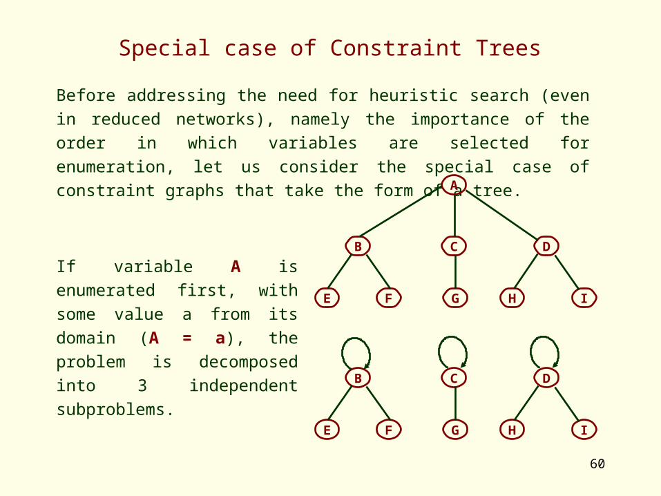
Special case of Constraint Trees

Before addressing the need for heuristic search (even in reduced

networks), namely the importance of the order in which variables are

selected for enumeration, let us consider the special case of constraint

graphs that take the form of a tree.

If variable A is enumerated first,

with some value a from its

domain (A = a), the problem is

decomposed into 3 independent

subproblems.

A

E

CB

GF

D

H I

E

CB

GF

D

H I

61


In this case, to guarantee that the enumeration does not lead

immediately to unsatisfiability, value a from variable A must have support

in variables B, C e D.

This reasoning may proceed recursively, for each of the subtrees with

roots B, C and D. For example, enumeration of B (say, B = b) does not

lead to an immediate “dead end” if value b has support in E and F.

E

CB

GF

D

H I

62


Hence, a good heuristic to select the variable to enumerate is choosing

variables in the root of the tree (or subtree).

A

E

CB

GF

D

H I

In general, if enumeration of the variables in the tree is made from root to

leaves, such enumeration will not lead to unsatisfiability if the values kept

in any node have support in their children nodes.

63


Although this is not the case in general constraint graphs, as seen

before, constraint trees that are arc consistent are also satisfiable.

In fact,

1. Using any heuristics that selects the roots of the tree and its

subtrees,

2. This choice never leads to contradiction, since they have always

support in their children,

3. Such support is recursively guaranteed until the leaves.

Moreover, this direccionality in the enumeration (from root to leaves)

enables the consideration of directed arc consistency, a weaker

criterion than full arc consistency, but sufficient to handle constraint

trees.

64


In the previous example, it is not

necessary that all values in the

domain of B, C and D have

support in the domain of A. The

only requirement is that all values

in the domain of A have

support in the domains of B, C

and D.

When a value is chosen for A,

constraints on A and its

descendents become unary, and

the values from the domains of B,

C and D are removed by simple

node consistency.

A

E

CB

GF

D

H I

E

CB

GF

D

H I

65

Directed Arc Consistency

In general, one may define a criterion of directed arc consistency if, in

contrast to what has been considered, we consider a directed graph to

represent the constraint network (assuming some direction to each

constraint of the problem).

Definition (Directed Arc Consistency):

A constraint problem is directed arc consistent iff

1. It is node consistent; and

2. For every label Xi-vi of any variable Xi, and for any directed arc

aij (from Xi to Xj) corresponding to a constraint Cij, there is a

supporting value vj in the domain of Xj, i.e. the compound label

{Xi-vi, Xj-vj} satisfies constraint Rij.

66

Maintaining Directed Arc Consistency: DAC

Maintaining Directed Arc Consistency

The algorithm below assumes that variables are “sorted” from 1 to n, and

there are only arcs from the “highest” to the “lowest” variable. It simply

enforces consistency in all directed arcs, starting with the highest

variables, without considering any further reexamination of the arcs.

procedure DAC(V, D, C); for i from n downto 1 do for Cij in C do

if i < j then revise_dom(aij,V,D,C) end if

end for end forend procedure

Note: revise_dom(aij,V,D,R) is that used in AC-1 e AC-3.

67


Algorithm DAC: Time Complexity

As usual, let us assume a arcs and that the n variables have d values

in their domain.

The algorithm visits each arc exactly once. For each arc aij, each of the

d values of variable Xi is tested with d values from variable Xj, in the

worst case.

All factors considered, and like in AC-4/6/7, the worst case time

complexity of algorithm DAC is O(ad2). However, in a tree a = n-1 (not

a n2) so the complexity of DAC is

O(nd2)

Moreover, the algorithm has no requirements regarding memory use

(space complexity).

68


As can be seen, algorithm DAC does not guarantee the elimination of all

redundant values, since it does not reexamine variables that could loose

support.

If in the general case this might be innadequate, this is not a problem in

the case of trees, if the arcs, which are directed in descending order of

the variables (the tree root has lowest number) are revised in

descending order, i.e. arcs closer to the leaves are revised first.

Then all the values of a node have guaranteed support in all the nodes

down to the leaves of a tree, although not necessarily on those upto the

tree root!

As shown before, if enumeration starts from the root, the unsupported

values are eliminated by node consistency.

69


Example: Take the constraint tree below

1

5

32

76

4

8 9

> >

>> > >>

>X1 in {1, 3, 5, 7, 9},

X2 in {2, 4, 6}, X5 in {4,8}, X6 in {3, 9},

X3 in {1, 5, 7}, X7 in {3, 9},

X4 in {1, 5, 8}, X8 in {3, 7}, X9 in {2, 9}

After revising arc X9 -> X4 X4 in {1, 5, 8} % X9 >= 2

X8 -> X4 X4 in {1, 5, 8} % X8 >= 3

X7 -> X3 X3 in {1, 5, 7} % X7 >= 3

X6 -> X2 X2 in {2, 4, 6} % X6 >= 3

X5 -> X2 X2 in {2, 4, 6} % X5 >= 4

X4 -> X1 X1 in {1, 3, 5, 7, 9} % X4 >= 5

X3 -> X1 X1 in {1, 3, 5, 7, 9} % X3 >= 5

X2 -> X1 X1 in {1, 3, 5, 7, 9} % X2 >= 6

70


Example (cont): The enumeration became backtrack free !

X1 in {7, 9},

X2 in {6}, X5 in {4, 8}, X6 in {3, 9},

X3 in {5, 7}, X7 in {3, 9},

X4 in {5, 8}, X8 in {3, 7}, X9 in {2, 9}

X1 = 7 NC enforces X2 in {6}, X3 in {5}, X4 in {5}

X2 = 6 NC enforces X5 in {4}, X6 in {3},

X3 = 5 NC enforces X7 in {3},

X4 = 4 NC enforces X8 in {3}, X9 in {2},

X1 = 9 NC enforces X2 in {6}, X3 in {5,7}, X4 in {4, 8}

X2 = 6 ...., X3 in {5,7}, enforces X7 = 3

X4 = 4 NC enforces X8 in {3}, X9 in {2}

or X4 = 8 NC enforces X8 in {3, 7}, X9 in {2}

1

5

32

76

4

8 9

> >

>> > >>

>

1 changes to ac-4 - algorithm ac-6 –algorithm ac-6 avoids the outlined inefficiency of ac-4 with a...

Documents

variable x

pairs x

x j v

pair x j

domain of x j

supportsno attack x

supported v

phases of ac