2016 Billion-Ton Report | 183

06 Water Quality Response to Forest Biomass Utilization

Benjamin Rau,1 Augustine Muwamba,2 Carl Trettin,3 Sudhanshu Panda,4 Devendra M. Amatya,3 and Ernest W. Tollner2

1 U.S. Department of Agriculture (USDA) Forest Service, Aiken, SC,2 College of Engineering, University of Georgia, Athens, GA, 3 USDA Forest Service, Cordesville, SC, 4 University of North Georgia, Oakwood, GA

WateR QUality Response to FoRest Biomass Utilization

184 | 2016 Billion-Ton Report

6.1 IntroductionForested watersheds provide approximately 80% of freshwater drinking resources in the United States (Fox et al. 2007). The water originating from forested watersheds is typically of high quality when compared to agricul-tural watersheds, and concentrations of nitrogen and phosphorus are nine times higher, on average, in agricultur-al watersheds when compared to forested watersheds (Fox et al. 2007). Silvicultural activities typically occur on a low percentage of forested lands in any one year, and effects on water quality from silvicultural operations are typically localized and short-lived (Bethea 1985; Dissmeyer 2000).

The effects of silvicultural activities on water quality have been reviewed on several occasions, and the findings are remarkably consistent. Throughout the United States, silvicultural activities have minimal effects on water quality, and potential effects from harvest operations are largely mitigated by the widespread adoption of best management practices (BMPs) (Binkley and Brown 1993; Fulton and West 2002; Grace III 2005; Stednick 2010; Ice et al. 2010). Silvicultural activities that may compromise water quality are typically nonpoint source and include road construction, ground disturbance from whole-tree skidding, mechanical site-preparation activi-ties, herbicide application, and fertilizer application (Fulton and West 2002).

In this chapter, we briefly review the current effects of silvicultural activities on water quality and then assess the potential effects of increased demand for biomass, based on select scenarios from the 2016 Billion-Ton Report (BT16), on several water-quality indicators including sediment, nitrate (NO3

-), and total phosphorus (TP) load. The literature documenting the specific effects of biomass removal from forests on water quality is sparse at best. However, the majority of biomass would be harvested using harvest systems that mimic current silvicul-tural practices. Therefore, it is reasonable to relate the potential effects of traditional forest-harvest operations to what we might expect from the removal of biomass.

2016 Billion-Ton Report | 185

6.1.1 Sediment, Nitrate, and TP Perhaps the most widespread and deleterious wa-ter-quality-related effect of silvicultural operations comes from the displacement of sediment and its transport into stream channels, particularly due to road construction, harvesting, and site preparation (Grace III 2005). The extent of erosion and sediment transport is based on several factors, including the soil texture, organic matter content, slope angle, and application of BMPs (Fulton and West 2002). Sediment impairs aquatic habitats by reducing water and gas exchange between the stream and the groundwater below and adjacent to it. Sediment also fills in pools and covers stream-bed gravels, which are critical to salmonid survival and reproduction (Waters 1995). Harvest operations, including road construction, log skidding, and site preparation, often expose bare soil and increase the risk of erosion. It has been estimated that up to 90% of sediment deliv-ered to streams following forest-harvest operations is road-related (Appelboom et al. 2002; Scoles et al. 1996). However, skidding logs across the soil surface exposes and compacts mineral soil, and may create furrows that channel overland flow (Fulton and West 2002). In addition to road construction and harvesting activities, mechanical site-preparation activities, such as shearing, disking, drum-chopping, and root-raking, cause significant soil disturbance, which can lead to further sediment transport after harvests (Fulton and West 2002). These activities were once common on pine plantations, which are widespread in the south-eastern United States (Grace III 2005), but chemical herbicides have increasingly replaced mechanical site-preparation activities as a more economical way to reduce competition. Sedimentation effects from silviculture are typically short-lived, lasting 2–5 years (one example is from Amatya et al. 2006) or until un-derstory vegetation has recovered in disturbed areas.

In healthy, undisturbed forest ecosystems, only a very small fraction of nutrients is lost to surface waters. Nutrient cycles in these systems are typically very

tight, with most nutrients being bound and efficient-ly cycled through vegetation and soils (Bormann and Likens 1994; Scoles et al. 1996). The removal of trees and understory vegetation during harvest activities can cause nutrient transport to streams to occur via leaching and erosion (Scoles et al. 1996). Nitrogen and phosphorus are the primary nutrients that influence ecological processes and productiv-ity in streams and lakes (Fulton and West 2002). Increased loading of nitrogen and phosphorus can cause increased biological activity, increased turbidi-ty, limited light penetration, and increased biological oxygen demand (Fulton and West 2002). The “eu-trophication” of surface waters by increased nutri-ent loading has significant effects on fish and other aquatic organisms.

Most forest-harvesting studies in the United States have demonstrated that stream-water nitrogen concentrations, including NO3

-, increase after har-vest, but stream-water concentrations of NO3

- rarely exceed the U.S. Environmental Protection Agency’s (EPA’s) drinking water standard of 10 milligrams per liter (mg/L) (Binkley and Brown 1993). More commonly, nitrate nitrogen (NO3

--N) increased up to 1 mg/L (Swank 1988; Askew and Williams 1986; Riekirk 1983; Hewlett, Post, and Doss 1984; Miller et al. 1988; Amatya et al. 2006). Within the literature, however, it has been documented that higher levels of stream-water nitrate may occur after harvest in areas prone to high levels of atmospheric nitrogen depo-sition, particularly in the northeastern United States (Likens et al. 1970; Bormann et al. 1968; Yanai 1998). Phosphorus has not been as thoroughly stud-ied within the context of forest harvest, but several studies describe a significant increase in TP immedi-ately following harvest (Blackburn and Wood 1990; Wynn et al. 2000; Amatya et al. 2006; McBroom et al. 2008). As with sediment, nitrogen and phosphorus typically increase the first year after harvesting but return to pre-harvest levels within 2–4 years follow-ing harvest (Shepard 1994; Amatya et al. 2006).

WateR QUality Response to FoRest Biomass Utilization

186 | 2016 Billion-Ton Report

6.1.2 Management Intensity and BMPsAlthough road building, road use, and related activ-ities account for the majority of silviculture-related effects on water quality (Grace III 2005), the inten-sity of management may also determine the extent of effects. Silvicultural methods vary widely in the amount of material harvested and the mechanical dis-turbance created by harvesting. Single-tree selection or group-selection harvests often remove significantly less biomass than clearcutting. The research findings that relate biomass removal to sediment and nutri-ent loads (loadings) are straightforward. For exam-ple, Beasley and Granillo (1985) demonstrated that selective harvests yielded significantly less sediment than clearcuts. However, in a study comparing four harvesting methods, including selective and clear-cutting, Eschner and Larmoyeux (1963) determined that neither the number/mass of trees removed nor the harvesting method utilized was the primary factor influencing water quality; rather, it was skid trail and logging-road design.

Mechanical site preparation after clearcutting has been demonstrated to increase sediment and phospho-rus loads, but less evidence supports significant in-creases in nitrate or total nitrogen loads (Amatya et al. 2006; Muwamba et al. 2015). Shearing, root raking, disking, and windrowing expose bare soil, decrease soil stability, and increase erosion rates. For example, Douglass (1977) determined that the amount of sedi-ment lost from sites that were cleared and disked was twice that from sites that were cleared only. Because phosphorus is often transported along with sediment as particulates, it may increase after site preparation as well. Blackburn and Wood (1990) observed that when shearing was used to remove stumps and wind-row debris, phosphate and TP increased significantly compared to treatments in which debris was chopped in place. With use of herbicides replacing mechanical methods for competition control, these effects should be reduced.

Intensive management of pine and Douglas-fir plan-tations increasingly involves herbicide and fertilizer application. The effect of herbicide application on sediment, nitrogen, and phosphorus in streams and lakes is likely minimal; however, it has been demon-strated that fertilization can temporarily increase am-monium, total nitrogen, ortho-phosphate, and TP in streams draining plantations (Fulton and West 2002; Beltran et al. 2010). The Binkley, Burnham, and Allen (1999) review of forest fertilization concluded that in the absence of BMPs, nitrate and phosphorus levels increased in receiving waters, drinking water standards were not exceeded, and the increase in nutrient levels was short-lived.

It has been widely demonstrated that BMPs are very effective at mitigating the effects of silvicultural operations on water quality (Grace III 2005). The most common and effective BMPs typically involve aspects of road design and utilization of riparian buffers. Because the majority of sediment intro-duced to stream channels from silvicultural activities is road-related, significant improvements in water quality can be made by employing road-design BMPs (Appelboom et al. 2002). Appelboom et al. (2002) showed that a continuous berm maintained along the edge of a forest road can reduce total sediment loss by an average of 99% compared to the same type of road without the presence of a continuous berm. When a continuous berm is not present, graveling the road surface can reduce the total loss of sedi-ment from roads by an average of 61% compared to a non-graveled road surface. An experiment at the Coweeta Watershed in western North Carolina demonstrated that sediment delivery to a stream channel can be reduced by up to 50% with proper planning and layout of roads and skid trails (Swift 1988). Similarly, Mostaghimi et al. (1999) report-ed that harvesting and intensive site preparation increased nitrogen and phosphorus loading where BMPs were not applied. Mostaghimi et al. (1999) also reported that use of BMPs mitigated the effects of harvesting and site preparation, while Vowell

2016 Billion-Ton Report | 187

(2001) reported that following state BMPs in Florida resulted in no significant increases in stream water nitrogen or phosphorus. An increasing body of evi-dence shows that silvicultural effects on water quality are relatively small and short-lived (Shepard 1994) when compared to agricultural practices, and proper implementation of BMPs can effectively mitigate most water-quality effects. In a recent survey of BMP implementation, Ice et al. (2010) estimated that BMP compliance in forestry is approaching 90% nationally.

The objective of the analysis that follows is to estimate the effects of forest-biomass removal on surface-water quality (sediment, NO3

--N, and TP) for select scenarios of BT16 (described in chapter 2) in the conterminous United States. The analysis focuses on three commonly reported harvest types: thinning operations, clearcuts with natural regeneration, and clearcuts with site preparation and planting (plan-tations). Water-quality estimates for the potential biomass supply are produced at the county level and aggregated to three regions having relatively unique climates and vegetation (DOE 2016).

6.2 MethodsTo assess the possible effects of potential forest-bio-mass removal on water quality, we searched the peer-reviewed literature for studies that either direct-ly reported effects on water quality from biomass removal or reported effects on water quality from traditional silvicultural operations. Within each paper, data were extracted detailing the forest vegetation type, stand age, basal area, geographic location, climate, topography, soil, harvest operations, the mass of material removed, pre-harvest water-quality

parameters, and changes in water quality follow-ing silvicultural operations. The initial goal was to develop a series of regionally specific models that would relate potential mass of biomass removed to changes in water quality; then, we could apply those models to the output derived from the Forest Sus-tainable and Economic Analysis Model (ForSEAM) for select biomass-removal scenarios proposed in the years 2017 and 2040 (DOE 2016). However, devel-oping significant, predictable relationships between biomass removal and water quality that could be applied regionally proved impossible given the lack of detailed information and relatively small number of studies available in the literature. Since it was not possible to develop a full suite of harvest-type and region-specific models relating biomass removal to water quality, we adopted an approach that relates the acres harvested to changes in water quality, and we developed regional or harvest-type-specific models when possible. All other models are general for the conterminous United States.

6.2.1 Scope of AssessmentThe scope of this assessment covers the incremental effects of biomass harvest activities on water quality for select scenarios described in BT16, volume 1 (DOE 2016). The scenarios include the baseline moderate housing–low wood energy demand (ML) scenario in 2017 and 2040, and an alternative high housing–high wood energy demand (HH) scenario in 2040. The scenarios and assumptions are de-scribed in chapter 2. For this assessment, results from ForSEAM are analyzed at the county level and then aggregated to three regions (North, South, and West) of the conterminous United States (fig. 6.1).

WateR QUality Response to FoRest Biomass Utilization

188 | 2016 Billion-Ton Report

assessment. When pre-harvest or control data were available, they were considered the reference con-dition. All data recorded after harvest treatments were considered the response to harvest. Units for reference and response conditions were expressed as kilograms of response variable delivered to a water body per hectare per measurement year (kg/ha/year). A generalized, linear mixed-effects model (Proc GLIMMIX, SAS 9.4, SAS Institute, Cary, North Car-olina) was used to determine harvest type and region-al differences in NO3

--N, TP, and sediment response to biomass removal. Because not all studies reported data for the same number of years post-harvest, only the initial response year was used for statistical com-parisons.

Figure 6.1 | Map showing states in the northern, southern, and western regions of the United States. Separate forest water quality analyses were undertaken for these regions.

WEST NORTH

SOUTH

6.2.2 Description of Water Quality Response ModelingWe searched peer-reviewed literature and identified 38 papers containing quantitative data describing the effects of forest harvest on water quality (table 6.1). Studies were separated into three categories for analysis: thinning operations; clearcuts with natural regeneration; and plantations where extensive site preparation, fertilization, and herbicide applications were used in conjunction with replanting trees. Table 6.2 details the silvicultural activities common to each harvest type. Sediment, NO3

--N, and TP were the three water-quality parameters selected for this

2016 Billion-Ton Report | 189

Citation Region State NO3--N TP Sediment

1. Bormann et al. (1968) North NH ●

2. Bormann et al. (1974) North NH ●

3. Briggs et al. (2000) North ME ●

4. Hornbeck et al. (1987) North NH ●

5. Hornbeck et al. (1990) North NH,ME,CT ● ●

6. Likens et al. (1970) North NH ●

7. Martin and Hornbeck (1994) North NH ●

8. Wang et al. (2006) North NY ●

9. Yanai (1998) North NH ● ●

10. Amatya et al. (2006) South NC ● ●

11. Amatya and Skaggs (2008) South NC ● ●

12. Arthur, Coltharp, and Brown (1998) South KY ●

13. Aubertin and Patric (1974) South VA ●

14. Beasley (1979) South MS ●

15. Beasley and Granillo (1988) South AR ●

16. Beasley, Granillo, and Zillmer (1986) South AR ●

17. Blackburn, Wood, and Dehaven (1986) South TX ●

18. Blackburn and Wood (1990) South TX ● ●

19. Chang, Roth, and Hunt (1982) South TX ●

20. Fox, Burger, and Kreh (1986) South VA ●

21. Grace III (2004) South AL ●

22. Grace III and Carter (2000) South AL ●

23. Grace III and Carter (2001) South AL ●

24. Grace III, Skaggs, and Chescheir (2006)

South NC ● ●

25. McBroom, Chang, and Sayok (2002) South TX ● ●

Table 6.1 | Peer-Reviewed Publications Used To Extract Water-Quality Parameters

WateR QUality Response to FoRest Biomass Utilization

190 | 2016 Billion-Ton Report

Citation Region State NO3--N TP Sediment

26. McBroom et al. (2008) South TX ● ● ●

27. Miller (1984) South OK ●

28. Muwamba et al. (2015) South NC

29. Sanders and McBroom (2013) South TX ●

30. Swank, Vose, and Elliott (2001) South NC ● ●

31. Van Lear et al. (1985) South SC ● ●

32. Wynn et al. (2000) South VA ● ●

33. Brown and Krigier (1971) West OR ●

34. Gravelle et al. (2009) West ID ●

35. Heede and King (1990) West AZ ●

36. Karwan, Gravelle, and Hubbart (2007) West ID ●

37. Martin and Harr (1988) West OR ●

38. Tiedemann, Quigley, and Anderson (1988)

West OR ●

The length of time required for water quality in the treated units to return to pre-harvest levels, or lev-els similar to controls, was defined as the response period. In most cases, the experiments were not of sufficient length to capture the full response period as many studies only reported 1–3 years of post-har-vest data. Post-harvest measurement periods ranged from 1 to 13 years in the literature searched (table 6.1). The total loading of sediment, NO3

--N, or TP delivered to a water body over the response period in excess of the reference condition was defined as the response load. To characterize the response load for each water-quality variable, the mean and 90% confi-dence intervals were calculated for each harvest type, region, and year post-harvest, where appropriate, as indicated by the results of the mixed model. The mean response load and confidence intervals for each

year (kilograms/hectare [kg/ha]) were plotted against the year after harvest, and a curve was fit to each data set. The resultant family of response curves was best represented by an exponential function of the form:

Equation 6.1:

y = a-b*x

In this equation, y is the water quality response (kg/ha), a is a constant representing the y-intercept, is the exponential decay rate, and x represents the year after harvest. Solving each equation for x, where the response curve intersects the pre-harvest condition, gives the modeled response period for each variable. Integrating each curve on the interval from 0 to the end of the modeled response period generates the total modeled response after harvest in kg/ha. The modeled response to harvest could then be applied to

2016 Billion-Ton Report | 191

the biomass output from ForSEAM. First, the number of hectares where whole-tree harvests for biomass occurred was summed within each county by harvest type for each scenario and year. Next, the appropriate response load was applied to each harvest type, and the total water-quality response load for each coun-

ty was calculated as the sum of all harvested acres (kg). Finally, the regional water-quality response to biomass harvest was calculated as the sum of all county-level response loads within each region and expressed in gigagrams (Gg).

Harvest typeRoad

building/ improvement

BMPsLog

skiddingResidue removal

Mechanical site preparation

Herbicide Fertilizer

Thin ● ● ● ●

Clearcut with natural regeneration

● ● ● ●

Plantation clearcut

● ● ● ● ● ● ●

Table 6.2 | Common Silvicultural Operations Conducted during Three Different Harvest Types

For comparative purposes, reference estimates of sed-iment, NO3

--N, and TP load were also produced using pre-harvest conditions for each region. We applied the pre-harvest water quality values to all forested acres within a county based on data from the National Land Cover Database and the U. S. Forest Service’s Forest Inventory and Analysis (FIA) data, and then calculated the sum of all water-quality values deliv-ered to a water body within each geographic region. This load is referred to as the regional reference load. Similarly, we applied the pre-harvest water quality val-ues to only the harvested acres within a county. This load is referred to as the pre-harvest reference load.

6.3 Results Results from the mixed model comparing regional and harvest-type differences indicate that sediment load was consistent across regions, but sediment load was significantly (α = 0.05) greater from plantations

when compared to naturally re-generated stands (P < 0.05). Conversely, NO3

--N loads (loadings) were greater in the North than in any other region (P < 0.05), and there were no significant (α = 0.05) differences between harvest types. There were no significant region or harvest-type effects for TP.

The load-response curves were generated from an-nual means, based on the results of the mixed model, and were best fit by the exponential decay function described in equation 6.1 (fig. 6.2). The modeled mean response period after harvest for sediment load from plantations across all regions was 4.4 years with an integrated response load of 8,798 kg/ha. By com-parison, the mean response period for sediment from non-plantation harvests across all regions was 8.8 years, but with a response load of only 2,881 kg/ha. Over the life of the rotation, typical average annual rates of sediment yield from agriculture are typically much higher.1 The mean response period for NO3

--N

1 Over a typical 30-year pine plantation rotation, the average sediment load delivered to a water body is 520 kg/ha/year if BMPs are utilized. Over a similar 30-year period, agricultural production with and without BMPs applied may produce 2,700 kg/ha/year and 18,000 kg/ha/year of sediment loading respectively (Hill 1991).

WateR QUality Response to FoRest Biomass Utilization

192 | 2016 Billion-Ton Report

in the northern region for all harvest types was 3.7 years, with a mean response load of 43 kg/ha. The mean response period for NO3

--N across all harvest types for the rest of the United States was 4.3 years with a mean response load of 6 kg/ha. For TP, the mean response time was 3.9 years, and the response load was 1.0 kg/ha across all regions and harvest types. Table 6.3 provides the full suite of coefficients of the fitted model, as well as related statistics for

means and 90% confidence intervals of response loads and periods.

Non-aggregated, county-scale graphical depictions of sediment, NO3

--N, and TP increases due to biomass harvest can be found in figures 6.3–6.5. The complete series of regional reference estimates, pre-harvest estimates, and increases due to biomass harvesting can be found in table 6.4.

2016 Billion-Ton Report | 193Year After Harvest

Year After Harvest

1

0.0

0.5

1.0

1.5

2.0

Mean Harvest Response

Mean Pre-Harvest Yield

32 5 64 7

1 32 5 64 7 1 32 5 64 7

Kg h

a-1Kg

ha-1

5

0

10

15

25

20

30

0

2

4

8

6

10

1 32 5 64 7

Mg

ha-1

0

2

4

8

6

10

1 32 5 64 70.0

0.5

2.0

1.5

1.0

2.5

Modeled Harvest Response

Upper 90% Prediction

Lower 90% Prediction

TP Yield (National)

NO3 Yield (North) NO3 Yield (South and West)

Sediment Yield (Plantation) Sediment Yield (Thin and CC)

Figure 6.2 | Sediment, NO3--N, and TP load response curves and the 90% prediction intervals generated from the

results of the mixed model comparing regions and harvest types. Bars represent the upper and lower 90% confi-dence limit for each mean in each year after harvest.

Acronym: CC – clearcut.

WateR QUality Response to FoRest Biomass Utilization

194 | 2016 Billion-Ton Report

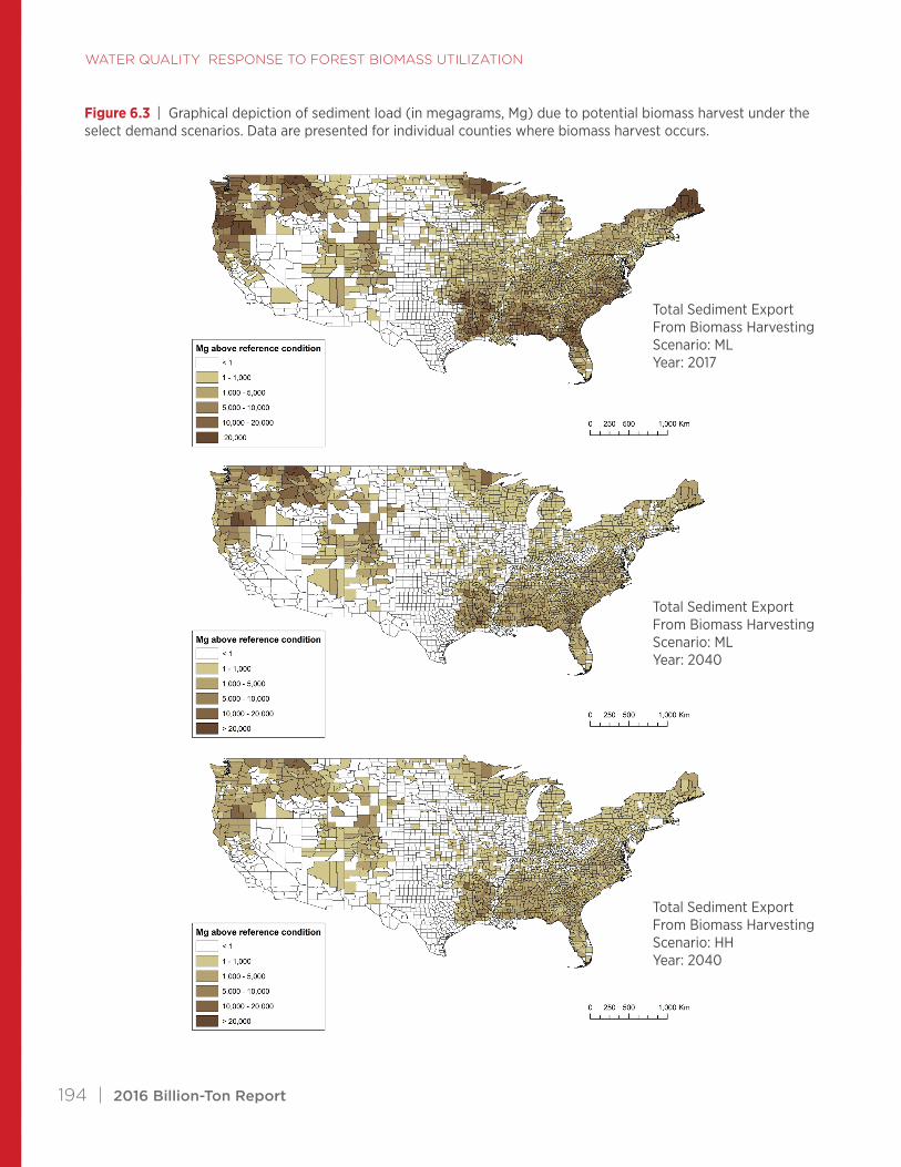
Figure 6.3 | Graphical depiction of sediment load (in megagrams, Mg) due to potential biomass harvest under the select demand scenarios. Data are presented for individual counties where biomass harvest occurs.

Total Sediment Export From Biomass Harvesting Scenario: ML Year: 2017

Total Sediment Export From Biomass Harvesting Scenario: ML Year: 2040

Total Sediment Export From Biomass Harvesting Scenario: HH Year: 2040

2016 Billion-Ton Report | 195

Figure 6.4 | Graphical depiction of nitrate load (in kg) due to potential biomass harvest under the select demand scenarios. Data are presented for individual counties where biomass harvest occurs.

Nitrate Export From Biomass Harvesting Scenario: ML Year: 2017

Nitrate Export From Biomass Harvesting Scenario: ML Year: 2040

Nitrate Export From Biomass Harvesting Scenario: HH Year: 2040

WateR QUality Response to FoRest Biomass Utilization

196 | 2016 Billion-Ton Report

Figure 6.5 | Graphical depiction of total phosphorus load (in kg) due to potential biomass harvest under the select demand scenarios. Data are presented for individual counties where biomass harvest occurs.

Total Phosphorus Export From Biomass Harvesting Scenario: ML Year: 2017

Total Phosphorus Export From Biomass Harvesting Scenario: ML Year: 2040

Total Phosphorus Export From Biomass Harvesting Scenario: HH Year: 2040

2016 Billion-Ton Report | 197

Response variable RegionCoefficient

aCoefficient

bR2 P-value

Response period (years)

Response load

integral (kg/ha)

Sediment plantation 90% LPL

National 3308.46 -1.17 0.98 0.0096 2.9 2,738

Sediment plantation mean

National 8971.63 -1.01 0.79 0.0104 4.4 8,798

Sediment plantation 90% UPL

National 14754.48 -0.98 0.98 0.0110 5.0 14,972

Sediment 90% LPL National 104.54 -0.01 0.00 0.9488 0.0 0

Sediment mean National 742.00 -0.22 0.66 0.0137 8.8 2,881

Sediment 90% UPL National 1288.38 -0.14 0.28 0.2850 18.2 8,686

NO3- 90% LPL Northern 23.86 -1.34 0.61 0.1171 1.6 16

NO3- mean Northern 31.77 -0.68 1.00 <0.0001 3.7 43

NO3- 90% UPL Northern 44.26 -0.54 0.95 0.0054 5.2 77

NO3- 90% LPL National 5.33 -1.47 0.89 0.0152 1.9 3

NO3- mean National 3.86 -0.57 0.90 0.0245 4.3 6

NO3- 90% UPL National 4.62 -0.39 0.73 0.0656 6.7 11

TP 90% LPL National 0.01 -0.04 0.17 0.4849 0.0 0

TP mean National 0.74 -0.61 0.78 0.0488 3.9 1

TP 90% UPL National 1.46 -0.50 0.56 0.1461 6.1 3

Table 6.3 | Parameters for the Mean and 90% Prediction Interval, Water-Quality Response Curves

Acronyms: LPL – lower prediction limit; UPL – upper prediction limit.

6.3.1 Baseline Scenario ML 2017Under the baseline scenario, in the year 2017, it is es-timated that sediment loading would be greatest from the southern region of the United States and that the mean sediment load of 4,300 Gg represents a 39% increase over the regional reference for sediment load from current forest management (table 6.4). Mean sediment load attributed to biomass harvest from the

northern region (1,400 Gg) and the western region (1,300 Gg) would be considerably lower than in the southern region and would represent 19% and 12% increases, respectively, over regional reference condi-tions derived from current forest management (table 6.4). Under the baseline 2017 scenario, total NO3

--N loading from biomass harvesting is estimated to be greatest from the northern region with an addition-al 15 Gg or 2% increase occurring on average over

WateR QUality Response to FoRest Biomass Utilization

198 | 2016 Billion-Ton Report

reference conditions (table 6.4). Total NO3--N load

from the southern (4 Gg) and western regions (2 Gg) represent 3% and 1% increases, respectively, over reference conditions (table 6.4). Similar to sediment, TP load from biomass harvesting is estimated to be greatest in the southern region, where an additional 0.9 Gg of TP would represent a 13% increase over reference conditions (table 6.4). TP load from bio-mass harvest in the ML 2017 scenario is estimated to be 0.5 Gg from the northern region and 0.4 Gg from the western region, or 10% and 13% increases, respectively, over reference conditions (table 6.4).

6.3.2 ML 2040 and HH 2040In 2040, under the ML scenario, sediment, NO3

--N, and TP delivery to water bodies due to biomass harvesting all decrease below the 2017 baseline. For instance, mean sediment load decreases to 1,800 megagrams (Mg) in the South, and to 700 Mg and 200 Mg in the West and North, respectively (table 6.4). These mean sediment loads are approximate-ly 16%, 7%, and 2% increases, respectively, over regional reference conditions (table 6.4). The main driver of this decrease in post-biomass-harvest load is the assumptions made in ForSEAM. The model assumes that no new land will be converted to planta-tion forestry in the southeastern United States—even if demand for wood products increases. Therefore, greater quantities of wood products are diverted to housing and other building supply chains rather than to biomass for energy. Under this scenario, NO3

--N load decreases to 2 Gg in the North, 1.6 Gg in the South, and 1.2 Gg in the West. All the decreases are ≤1% above regional references (table 6.4). Similarly, total post-biomass-harvest loads for TP were obtained as 0.4 Gg in the South, 0.3 Gg in the West, and 0.1 Gg in the North (table 6.4).

The HH scenario results in a further reduction of biomass-harvest-related sediment, NO3

--N, and TP loads in 2040 (fig. 6.6). Under this scenario, signif-icant wood resources are diverted into housing, and

demand for biomass cannot be met. The sediment load attributable to biomass harvest in the South falls to 1,100 Gg and to 300 Gg and 100 Gg in the West and North, respectively (table 6.4), which represent 10%, 3%, and 1% increases over regional reference conditions (table 6.4). Under the HH 2040 scenario, NO3--N is actually higher in the South compared to the North and West, but decreases to 1.3 Gg while loads in the North and West are 1.1 Gg and 0.5 Gg, respectively (table 6.4). All NO3

--N loads in this scenario represent ≤1% increase over reference conditions (table 6.4). TP loads from biomass harvest under the HH 2040 scenario are highest in the South, but are well below 1 Gg in each region, as shown in figure 6.6. TP loads are 4% in excess of reference values in the South, 2% over reference in the West, and 1% over regional reference in the North (table 6.4).

6.4 DiscussionThe water-quality estimates obtained using the empir-ical models derived from the peer-reviewed literature and applied to potential biomass utilization in select scenarios show there could be regional variation in how biomass harvest would influence water quality. Sediment loads often increase after intensive site preparation in plantations. Because these practices are most common in the South, our estimates indicate that absolute sediment loads and percent increases over reference conditions would be greatest in the South, with smaller increases in the West and North. Alternatively, estimates indicate that absolute NO3

-

-N loads would increase most in the North, but when considered as an increase over regional reference, the highest increase occurs in the South, followed by the North and then the West in ML 2017. In the ML 2040 and HH 2040 scenarios, the largest percent increase is still estimated to be in the South, but the West surpasses the North (table 6.4). The pattern observed is likely due to two factors. The northern region of the United States, where many of the peer-reviewed

2016 Billion-Ton Report | 199

studies of harvest effects on nutrient and sediment load were conducted, has a long legacy of atmospher-ic nitrogen deposition from industrial processes. This legacy has led to increased reference concentrations of NO3

--N in much of the region. When vegetation is removed from forests in the region, temporary spikes in NO3

--N are common due to reduced plant uptake. However, because the reference-load values are large, their increase after harvest may be relatively small when considered as a percentage of total load. In contrast, the South and West reference NO3

--N loads are lower, so changes after harvest can be a larger percentage of total loads. The changes in regional NO3

--N loads over time in alternative biomass-de-mand scenarios occur due to the dynamic nature of ForSEAM, which models supply and demand at the regional scale as well. Because a single model was applied for TP response to all biomass harvests, the estimated regional differences in TP response to biomass harvest and change over time, as well as intensity, are solely due to the forested acres within a region and the supply and demand for biomass.

The estimated response to biomass harvest indicates that sediment flux is the most dynamic water-quality parameter; sediment flux typically increases after

harvests, particularly in areas where mechanical site preparation is common prior to planting. However, chemical herbicides are becoming economically viable and effective alternatives to mechanical site preparation for controlling competition during the early stages of plantation development. If this trend of increasing herbicide use continues, then sediment loads are likely to decrease below what has been estimated here. The estimated responses for NO3

--N and TP tend to be less dynamic and typically re-sult in <10% increase over reference loads. For all water-quality parameters, the load-response period is typically <5 years. Silvicultural activities generally occur on relatively few acres each year compared to the total forested acres within any given watershed, and activities typically only occur on the same tract of land once during a stand rotation. Therefore, the effects of silvicultural activities on water quality are typically small when compared to current agricultural activities involving annual crops (on a per-area ba-sis); which typically occur multiple times each year on the same tract of land (Shepard 1994). Continued adherence to and increased adoption of BMPs on lands on which silviculture is practiced should mini-mize biomass-harvest effects.

WateR QUality Response to FoRest Biomass Utilization

200 | 2016 Billion-Ton Report

Table 6.4 | Mean Region Reference Load, Pre-Harvest Load, and the Increase over Reference Load after Biomass Harvest Expressed as Total Regional Flux and a Percentage of Reference Load with Lower (LPL) and Upper (UPL) 90% Prediction Limits.

Raw Values Increase over Pre-Harvest % Change over Regional Baseline

Scenario Year RegionSed. Region

Baseline (Gg)Sed. Pre-

Harvest (Gg)Sed. LPL

(Gg)Sed. Mean

(Gg)Sed. UPL

(Gg)Sed. LPL Sed. Mean Sed. UPL

ML 2017 North 7,400 50 60 1,400 4,000 0.8% 19% 54%

ML 2017 South 11,000 100 810 4,300 9,600 7% 39% 87%

ML 2017 West 10,200 40 130 1,300 3,300 1% 12% 32%

ML 2040 North 7,400 10 4 200 500 0.1% 2% 7%

ML 2040 South 11,000 40 360 1,800 3,800 3% 16% 34%

ML 2040 West 10,200 30 2 700 2,200 0.0% 7% 22%

HH 2040 North 7,400 4 3 100 300 0.0% 1% 4%

HH 2040 South 11,000 30 180 1,100 2,700 2% 10% 25%

HH 2040 West 10,200 10 0 300 1,000 0.0% 3% 10%

Raw Values Increase over Pre-Harvest % Change over Regional Baseline

Scenario Year Region NO3- Region

Baseline (Gg)NO3

- Pre- Harvest (Gg)

NO3- LPL

(Gg)NO3

- Mean (Gg)

NO3- UPL

(Gg) NO3- LPL NO3

- Mean NO3- UPL

ML 2017 North 670 4.4 2.7 15.1 30.4 0.4% 2% 5%

ML 2017 South 150 1.3 1.7 4.2 8.5 1.2% 3% 6%

ML 2017 West 140 0.5 0.7 1.6 3.3 0.5% 1% 2%

ML 2040 North 670 0.6 0.4 2.0 4.0 0.1% 0.3% 0.6%

ML 2040 South 150 0.5 0.7 1.6 3.3 0.5% 1.1% 2.2%

ML 2040 West 140 0.4 0.5 1.2 2.5 0.4% 0.9% 2%

HH 2040 North 670 0.3 0.2 1.1 2.3 0.0% 0.2% 0.3%

HH 2040 South 150 0.4 0.5 1.3 2.5 0.4% 1% 2%

HH 2040 West 140 0.2 0.2 0.5 1.1 0.2% 0.4% 0.8%

Acronym: Sed. = sediment

2016 Billion-Ton Report | 201

Raw Values Increase over Pre-Harvest % Change over Regional Baseline

Scenario Year Region TP Region Baseline (Gg)

TP Pre- Harvest (Gg)

TP LPL (Gg)

TP Mean (Gg)

TP UPL (Gg) TP LPL TP Mean TP UPL

ML 2017 North 4.7 0.03 0.0 0.5 1.2 0.0% 10% 26%

ML 2017 South 7.0 0.06 0.0 0.9 2.4 0.0% 13% 34%

ML 2017 West 6.5 0.02 0.0 0.4 0.9 0.0% 6% 14%

ML 2040 North 4.7 0.00 0.0 0.1 0.2 0.0% 1% 3%

ML 2040 South 7.0 0.02 0.0 0.4 0.9 0.0% 5% 13%

ML 2040 West 6.5 0.02 0.0 0.3 0.7 0.0% 4% 11%

HH 2040 North 4.7 0.00 0.0 0.03 0.1 0.0% 1% 2%

HH 2040 South 7.0 0.02 0.0 0.3 0.7 0.0% 4% 10%

HH 2040 West 6.5 0.01 0.0 0.1 0.3 0.0% 2% 5%

6.5 Uncertainties and LimitationsWithin the vast body of silviculture-based literature reviewed, only 38 studies could be identified that reported sediment and nutrient loading to a body of water. Fewer than 10% of those studies identi-fied sites monitored long enough to determine that sediment and nutrient loads after harvest had returned to pre-harvest levels, defined here as the response period. Therefore, the mean load responses for the response periods were modeled, and 90% prediction intervals were determined to illustrate the ranges of possible responses as uncertainties in estimates (fig. 6.2 and table 6.3). Within the literature selected for this study, not all publications measured all variables of interest. The number of publications reporting data for sediment, NO3

--N, and TP were, 24, 20, and 9, re-spectively. Similarly, the number of studies found for each region was not equal, with 23 studies represent-

ing the South, 9 from the North, and 6 from the West. In addition, not all studies reported data for the same number of years post-harvest. Furthermore, harvest type was not represented evenly, and within each re-gion, there were differences in stocking rates, harvest rates, soil type, slope, aspect, vegetation type, and climate between studies. This resulted in an uneven number of data points for each variable and statistical uncertainty in computed parameters. To test the appli-cability of the model for load response, mean abso-lute error (MAE) and root mean square error (RMSE) (Chai and Draxler 2014) were calculated using the data reported from the literature and estimated values (table 6.5). The magnitude of the MAE and RMSE values was found to be minimal for NO3

--N and TP. However, the MAE and RMSE for sediment were relatively high, perhaps due to the variability of man-agement operations used to manipulate surface soil. We acknowledge that there may be other studies that were not examined in this analysis that may influence the statistics and model estimates.

WateR QUality Response to FoRest Biomass Utilization

202 | 2016 Billion-Ton Report

Parameter MAE-Reference RMSE-Reference MAE-Treatment RMSE-Treatment

NO3--N 1.420 1.800 0.020 0.030

TN 0.002 0.002 0.002 0.002

TP -0.001 0.001 -0.003 0.003

Sediment -0.002 0.002 729.5 1,029.8

Table 6.5 | Mean Absolute Error (MAE) and Root Mean Square Error (RMSE) for Literature-Derived Data and Projected Load-Response Value Comparisons

Acronym: TN – total nitrogen.

Because ForSEAM was used to generate the potential biomass and acres harvested under each scenario, our estimates of changes to water quality from biomass harvest are subject to the assumptions and limitations of ForSEAM as well. In particular, the assumption that no new plantations will be established in the southern United States drives the trend in decreasing sediment and nutrient load with increasing demand for wood products. As demand for wood products increases in the housing sector, less biomass is available for energy production, and therefore, less sediment and nutrient load is attributable to biomass harvests.

The values for sediment, NO3--N, and TP present-

ed here are only meant to represent the additional response to harvesting biomass, and they do not include the effects of associated harvests for other wood products; therefore, the results are incremen-tal. Similarly, the additional sediment and nutrient load produced by biomass harvest is compared to a reference considering pre-harvest forest watershed conditions and does not include any discharges due to concurrent silviculture, agriculture, or other activi-ties.

6.6 Summary and Future ResearchOur objectives were to utilize select scenarios from BT16 to estimate the effects of potential forest biomass removal on water quality at regional scales. However, the data available from peer-reviewed literature were not sufficient to warrant multivariate models relating biomass harvested to changes in water quality. Therefore, a simple, empirical mod-eling approach was developed to estimate sediment and nutrient response to the total acres estimated to be harvested for biomass within a given county, and then, results were aggregated to three regions of the United States.

This simple modeling approach produces a wide range of potential outcomes because of high levels of uncertainty associated with both the derived models and each data point within the model. This is partic-ularly true for sediment load. Despite this limitation, the results offer an initial estimate of the magnitude of possible effects relative to current forestry and agricultural practices. For example, sediment load for biomass harvesting from plantation forestry is estimated to be less than 9 Mg/ha over 4.4 years. On

2016 Billion-Ton Report | 203

an average annual basis, this sediment loading rate is about 20% of rates associated with agriculture with BMPs2 and about 3% of rates associated with agri-culture without BMPs (Hill 1991).

A process-based modeling approach would likely be most appropriate for this task, because there are nearly infinite combinations of soil type, topography, climate, vegetation, and harvest systems involved in estimating water-quality response to biomass harvests. However, at this time, very limited pro-cess-based modeling platforms are available to conduct large-scale distributed modeling of silvicul-tural activities (Amatya et al. 2013). It is imperative that forest-sector field researchers collaborate with engineers and modelers to develop, parameterize, and test process-based models for silvicultural activities. Rather than starting from scratch, it may be worth-while to utilize platforms from the agricultural sector as Amatya et al. (2013) did when modeling the fate of nitrogen in forest ecosystems.

Often, silviculture is not the only use of land within a watershed, and silvicultural effects on water quality are not isolated. It is critical that we begin to model watersheds with multiple land uses so that silvicul-

ture, agriculture, urban, and other land uses can all be integrated to estimate cumulative effects while assessing their individual effects as well.

Additional research is also needed to fill in the gaps in the existing literature. Where possible, long-term watershed-scale research should continue to deter-mine the effects of traditional and emerging silvicul-tural practices on water quality. Based on findings from this study, additional studies from the West, In-termountain West, Upper Midwest, North, and South states would fill in gaps in the knowledge base. There are several established experimental forests and watersheds throughout the United States. Many of these sites have been monitored for extended periods of time (Amatya et al. 2016). To maximize the value of these research installations, a coordinated series of experiments could be implemented to determine how emerging silvicultural practices, including biomass utilization, interact with variable climate and soils to influence water quality. These experiments could be modeled after the Long-Term Soil Productivity Experiment or the Long-Term Agricultural Research Network and could incorporate periodic herbicide application, fertilization, and thinning, or multiple rotations.

2 BMPs commonly utilized in agriculture include cover cropping, no-till or reduced tillage practices, contour cropping, crop rota-tions, perennial grass or forested riparian filter strips, grass swales, sediment detention basins, retention ponds, wetland basins, as well as manufactured media filters and porous pavement.

WateR QUality Response to FoRest Biomass Utilization

204 | 2016 Billion-Ton Report

6.7 ReferencesAmatya, D. M., J. Campbell, P. Wohlgemuth, K. Elder, S. Sebestyen, M. B. Adams, E. Keppler, S. Johnson, P.

Caldwell, and D. Misra. 2016 (in press). “Hydrological Processes of Reference Watershed in Experimental Forests, USA.” In Forest Hydrology: Processes, Management, and Applications. Edited by D. M. Amatya, T. M. Williams, L. Bren, and C. de Jong. Boston, MA: CAB International. http://www.srs.fs.usda.gov/pubs/chap/chap_2016_amatya_001.pdf.

Amatya, D. M., C. G. Rossi, Z. Dai, R. Williams, A. Saleh, M. A. Youssef, G. M. Chescheir, R. W. Skaggs, C. C. Trettin, E. Vance, and J. E. Nettles. 2013. “Modeling the Fate of Nitrogen Applied to Forest Ecosystems – An Assessment of Model Capabilities and Potential Applications.” Transactions of the American Society of Agricultural and Biological Engineers 56 (5): 1731–57.

Amatya D. M., and R. W. Skaggs. 2008. “Effects of Thinning on Hydrology and Water Quality of a Drained Pine Forest in Coastal North Carolina.” In Proceedings of the Conference on 21st Century Watershed Technology: Improving Water Quality and Environment: March 29–April 3, 2008. St. Joseph, MI: Ameri-can Society of Agricultural and Biological Engineers. ASABE Publication Number 701P0208cd.

Amatya, D. M., R. W. Skaggs, C. D. Blanton, and J. W. Gilliam. 2006. “Hydrologic and Water Quality Effects of Harvesting and Regeneration of a Drained Pine Forest.” In Proceedings of the ASABE, International Conference on Hydrology and Management of Forested Wetlands, New Bern, North Carolina, April 8–12, 2006. Edited by Williams and Nettles. St. Joseph, MI: American Society of Agricultural and Biological Engineers.

Appelboom, T. W., G. M. Chescheir, R. W. Skaggs, and D. L. Hesterberg. 2002. “Management Practices for Sediment Reduction from Forest Roads in the Coastal Plains.” Transactions of the American Society of Agricultural Engineers 45(2): 337–44. doi:10.13031/2013.8529.

Askew, G. R., and T. M. Williams. 1986. “Water Quality Changes Due to Site Conversion in Coastal South Car-olina.” Southern Journal of Applied Forestry 10(3): 134–6. http://docserver.ingentaconnect.com/deliver/connect/saf/01484419/v10n3/s7.pdf.

Aubertin, G. M., and J. H. Patric. 1974. “Water Quality after Clearcutting a Small Watershed in West Virginia.” Journal of Environmental Quality 3(3): 243–9. http://www.as.wvu.edu/fernow/Assests/Fernow%20Papers/Aubertin%20and%20Patric%201974%20Water%20quality%20in%20WS%203%20Fernow%20after%20clearcutting.pdf.

Arthur, M. A., G. B. Coltharp, and D. L. Brown. 1998. “Effects of Best Management Practices on Forest Stream Water Quality in Eastern Kentucky.” Journal of the American Water Resources Association 34(3): 481–95. doi:10.1111/j.1752-1688.1998.tb00948.x..

Beasley, R. S. 1979. “Intensive Site Preparation and Sediment Losses on Steep Watersheds in the Gulf Coastal Plain.” Soil Science Society of America Journal 43(2): 412–7. doi:10.2136/ss-saj1979.03615995004300020036x.

Beasley, R. S., and A. B. Granillo. 1985. “Water Yields and Sediment Losses from Chemical and Mechanical Site Preparation in Southwest Arkansas.” In Proceedings of Forestry and Water Quality: A Mid-South Symposium. Edited by B. G. Blackmon. Little Rock, AR: University of Arkansas at Monticello, 106–116.

2016 Billion-Ton Report | 205

———. 1988. “Sediment and Water Yields from Managed Forests on Flat Coastal Plain Sites.” American Water Resources Association 24(2): 361–6. doi:10.1111/j.1752-1688.1988.tb02994.x.

Beasley, R. S., A. B. Granillo, and V. Zillmer. 1986. “Sediment Losses from Forest Management: Mechani-cal vs. Chemical Site Preparation after Clearcutting.” Journal of Environmental Quality 15(4): 413–6. doi:10.2134/jeq1986.00472425001500040018x.

Beltran, B., D. M. Amatya, M. A. Youssef, M. Jones, R. W. Skaggs, T. J. Callahan, and J. E. Nettles. 2010. “Im-pacts of Fertilization Additions on Water Quality of a Drained Pine Plantation in North Carolina: A Worst Case Scenario.” Journal of Environmental Quality, 39(1): 293–303. doi:10.2134/jeq2008.0506.

Bethea, J. M. 1985. “Perspectives on Nonpoint Source Pollution Control: Silviculture.” In Proceedings from Perspectives on Nonpoint Source Pollution. Washington, DC: U.S. Environmental Protection Agency, Office of Water Regulations and Standards, 13. http://digitalcommons.brockport.edu/cgi/viewcontent.cgi?article=1072&context=wr_misc.

Binkley, D., and T. C. Brown. 1993. “Forest Practices as Nonpoint Sources of Pollution in North America.” Water Resources Bulletin 29(5): 729–40. doi:10.1111/j.1752-1688.1993.tb03233.x.

Binkley, D., D. H. Burnham, and H. L. Allen. 1999. “Water Quality Impacts of Forest Fertilization with Nitrogen and Phosphorus.” Forest Ecology and Management 121: 191–213. doi:10.1016/S0378-1127(98)00549-0.

Blackburn W. H., and J. C. Wood. 1990. “Nutrient Export in Storm Flow Following Forest Harvesting and Site-Preparation in East Texas.” Journal of Environmental Quality 19: 402–40. doi:10.2134/jeq1990.00472425001900030009x.

Blackburn W. H., J. C. Wood, and M. D. Dehaven. 1986. “Storm Flow and Sediment Losses from Site-Prepared Forestland in East Texas.” Water Resources Research 22(5): 776–84. doi:10.1029/WR022i005p00776.

Briggs, R. D., J. W. Hornbeck, C. T. Smith, R. C. Lemin Jr., and M. L. McCormack Jr. 2000. “Long-Term Ef-fects of Forest Management on Nutrient Cycling in Spruce-Fir Forests.” Forest Ecology and Management 138(1–3): 285–99. doi:10.1016/S0378-1127(00)00420-5.

Bormann, F. H., and G. E. Likens. 1994. “Pattern and Process in a Forested Ecosystem: Disturbance, Develop-ment, and the Steady State Based on the Hubbard Brook Ecosystem Study.” New York: Springer-Verlag, 253.

Bormann, F. H., G. E. Likens, D. W. Fisher, and R. S. Pierce. 1968. “Nutrient Loss Accelerated by Clear-Cutting of a Forest Ecosystem.” Science 159(3817): 882–4. doi:10.1126/science.159.3817.882.

Bormann, F. H., G. E. Likens, T. G. Siccama, R. S. Pierce, and J. S. Eaton. 1974. “The Export of Nutrients and Recovery of Stable Conditions Following Deforestation at Hubbard Brook.” Ecological Monographs 44(3): 255–77. doi:10.2307/2937031.

Brown, G. W., and J. T. Krygier. 1971. “Clear-Cut Logging and Sediment Production in the Oregon Coast Range.” Water Resources Research 7(5): 1189–98. doi:10.1029/WR007i005p01189.

Chai, T., and R. R. Draxler. 2014. “Root Mean Square Error (RMSE) or Mean Absolute Error (MAE)? – Ar-guments against Avoiding RMSE in the Literature.” Geoscientific Model Development 7: 1247–50. doi:10.5194/gmd-7-1247-2014.

WateR QUality Response to FoRest Biomass Utilization

206 | 2016 Billion-Ton Report

Chang, M., F. A. Roth II, and E. V. Hunt Jr. 1982. “Sediment Production under Various Forest-Site Conditions.” In Proceedings of the Exeter Symposium, July 1982. IAHS Publ. no. 137.

Dissmeyer, G. E., ed. 2000. Drinking Water from Forests and Grasslands: A Synthesis of the Scientific Liter-ature. Asheville, NC: U.S. Department of Agriculture, Forest Service, Southern Research Station, 246. General Technical Report SRS-39. http://www.srs.fs.fed.us/pubs/gtr/gtr_srs039/gtr_srs039.pdf.

DOE (U.S. Department of Energy). 2016. 2016 Billion-Ton Report: Advancing Domestic Resources for a Thriving Bioeconomy, Volume 1: Economic Availability of Feedstocks. Oak Ridge, TN: DOE, Oak Ridge National Laboratory. ORNL/TM-2016/160. http://energy.gov/sites/prod/files/2016/07/f33/2016_billion_ton_report_0.pdf.

Douglass, J. E. 1977. “Site Preparation Alternatives: Quantifying Their Effects on Soil and Water Resources.” In Proceedings of Site Preparation Workshop. East Raleigh, NC: U.S. Department of Agriculture, Forest Service.

Eschner, A. R., and J. Larmoyeux. 1963. “Logging and Trout: Four Experimental Forest Practices and Their Effect on Water Quality.” Progress in Fish Culture 25(2): 59–67. doi:10.1577/1548-8659(1963)25[59:LAT]2.0.CO;2.

Fox, T. R., H. L. Allen, T. J. Albaugh, R. Rubilar, and C. A. Carlson. 2007. “Forest Fertilization and Water Quality in the United States.” Better Crops 91(1): 1–9. http://www.ipni.net/publication/bettercrops.nsf/0/C48C93C1AA7B6B73852579800081D70C/$FILE/Better%20Crops%202007-1%20p7.pdf.

Fox, T. R., J. A. Burger, and R. E. Kreh. 1986. “Effects of Site Preparation on Nitrogen Dynamics in the South-ern Piedmont.” Forest Ecology and Management 15(4): 241–56. doi:10.1016/0378-1127(86)90162-3.

Fulton, S., and B. West. 2002. “Chapter 21: Forestry Impacts on Water Quality.” In Southern Forest Resource Assessment. Edited by D. N. Wear and J. G. Greis. Asheville, NC: U.S. Department of Agriculture, Forest Service, Southern Research Station, 501–18. General Technical Report SRS-53.

Grace III, J. M. 2004. “Soil Erosion Following Forest Operations in the Southern Piedmont of Central Al-abama.” Journal of Soil and Water Conservation 59(4): 160–6. http://www.srs.fs.usda.gov/pubs/ja/ja_grace013.pdf.

Grace III, J. M., 2005. “Forest Operations and Water Quality in the South.” Transactions of the American Soci-ety of Agricultural Engineers 48(2): 871–80. http://www.srs.fs.usda.gov/pubs/9454.

Grace III, J. M., and E. A. Carter. 2000. “Impact of Harvesting on Sediment and Runoff Production on a Pied-mont Site in Alabama.” Presented at 2000 ASAE Annual International Meeting. Paper No. 005019. 1–11. http://www.srs.fs.usda.gov/pubs/ja/ja_grace002.pdf.

Grace III, J. M., and E. A. Carter. 2001. “Sediment and Runoff Losses following Harvesting/Site Prep Opera-tions on a Piedmont Soil in Alabama.” In Proceedings of the 2001 American Society of Agricultural Engi-neers Annual International Meeting, July 30–August 1, 2001, Sacramento, CA. St. Joseph, MI: American Society of Agricultural and Biological Engineers, 1–9. Paper Number: 01-8002. http://www.srs.fs.usda.gov/pubs/ja/ja_grace006.pdf?.

2016 Billion-Ton Report | 207

Grace III, J. M., R. W. Skaggs, and G. M. Chescheir. 2006. “Hydrologic and Water Quality Effects of Thinning and Loblolly Pine.” Transactions of the American Society of Agricultural and Biological Engineers 49(3): 645−54. http://www.srs.fs.usda.gov/pubs/ja/ja_grace027.pdf.

Gravelle, J. A., G. Ice, T. E. Link, and D. L. Cook. 2009. “Nutrient Concentration Dynamics in an Inland Pacific Northwest Watershed before and after Timber Harvest.” Forest Ecology and Management 257: 1663–75. doi:10.1016/j.foreco.2009.01.017.

Heede, B. H., and R. M. King. 1990. “State-of-the-Art Timber Harvest in an Arizona Mixed Conifer Forest Has Minimal Effect on Overland Flow and Erosion.” Hydrological Sciences Journal 35(6): 623–35. doi:10.1080/02626669009492468.

Hewlett, J. D., H. E. Post, and R. Doss. 1984. “Effect of Clear-Cut Silviculture on Dissolved Ion Export and Water Yield in the Piedmont.” Water Resources Research 20: 1030–8. doi:10.1029/WR020i007p01030.

Hill, C. L. 1991. Effects of Land-Management on Sediment Yields in Northeastern Guilford County, North Car-olina. Raleigh, NC: U.S. Geological Survey. Water-Resources Investigations Report 90-4127. http://pubs.usgs.gov/wri/1990/4127/report.pdf.

Hornbeck. J. W., C. T. Smith, Q. W. Martin, L. M. Tritton, and R. S. Pierce. 1990. “Effect of Intensive Har-vesting on Nutrient Capitals of Three Forest Types in New England.” Forest Ecology and Management 30(1–4): 55–64. doi:10.1016/0378-1127(90)90126-V.

Hornbeck. J. W., C. W. Martin, R. S. Pierce, F. H. Bormann, G. E. Likens, and J. S. Eaton. 1987. The Northern Hardwood Forest Ecosystem: Ten Years of Recovery from Clearcutting. Broomall, PA: U.S. Department of Agriculture, Forest Service, Northeastern Forest Experiment Station, 30. NE-RP-596. http://www.fs.fed.us/ne/newtown_square/publications/research_papers/pdfs/scanned/OCR/ne_rp596.pdf.

Ice, G., M. McBroom, and P. Schweitzer. 2010. “A Review of Best Management Practices for Forest Watershed Biomass Harvests with an Emphasis on Recommendations for Leaving Residual Wood Onsite.” Oak Ridge, TN: Center for Bioenergy Sustainability, Oak Ridge National Laboratory. http://web.ornl.gov/sci/ees/cbes/Watershed/Review%20of%20BMPs%20Final%206%2030%202011.pdf.

Karwan, D. L., J. A. Gravelle, and J. A. Hubbart. 2007. “Effects of Timber Harvest on Suspended Sediment Loads in Mica Creek, Idaho.” Forest Science 53(2): 181–8. https://www.researchgate.net/publica-tion/228931533_Effects_of_timber_harvest_on_suspended_sediment_loads_in_Mica_Creek_Idaho.

Likens, G. E, F. H. Bormann, N. M. Johnson, D. W. Fisher, and R. S. Pierce. 1970. “Effects of Forest Cutting and Herbicide Treatment on Nutrient Budgets in the Hubbard Brook Watershed-Ecosystem.” Ecological Society of America, Ecological Monographs 40(1): 23–47. doi:10.2307/1942440.

Martin, C. C., and J. W. Hornbeck. 1994. “Logging in New England Need Not Cause Sedimentation of Streams.” Northern Journal of Applied Forestry 11(1): 17–23. http://www.ingentaconnect.com/content/saf/njaf/1994/00000011/00000001/art00005.

Martin, C. W., and R. D. Harr. 1988. “Logging of Mature Douglas-Fir in Western Oregon Has Little Effect on Nutrient Output Budgets.” Canadian Journal of Forest Research 19: 35–43. doi:10.1139/x89-005.

WateR QUality Response to FoRest Biomass Utilization

208 | 2016 Billion-Ton Report

McBroom, M. W., R. S. Beasley, M. Chang, and G. G. Ice. 2008. “Storm Runoff and Sediment Losses from Forest Clear Cutting and Stand Re-Establishment with Best Management Practices in East Texas, USA.” Hydrological Processes 22(10): 1509–22. doi:10.1002/hyp.6703.

McBroom, M. W., M. Chang, and A. K. Sayok. 2002. Forest Clearcutting and Site-Preparation on a Saline Soil in East Texas: Impacts on Water Quality. Nacogdoches, TX: Stephen F. Austin State University, Faculty Publications, 535–542. Paper 201.

Miller, E. L., R. S. Beasley, and E. R. Lawson. 1988. “Forest Harvest and Site Preparation Effects on Ero-sion and Sedimentation in the Ouachita Mountains.” Journal of Environmental Quality 17(2): 219–25. doi:10.2134/jeq1988.00472425001700020010x.

Miller, E. L. 1984. “Sediment Yield and Storm Flow Response to Clear-Cut Harvest and Site Preparation in the Ouachita Mountains.” Water Resource Research 20(4): 471–5. doi:10.1029/WR020i004p00471.

Mostaghimi, S., T. M. Wynn, J. W. Frazee, P. W. McClellan, R. M. Shaffer, and W. M. Aust. 1999. Effects of Forest Harvesting Best Management Practices on Surface Water Quality in the Virginia Coastal Plain. Rep. Blacksburg, VA: Virginia Polytechnic Institute and State University, Biological Systems Engineering. FNC0999.

Muwamba, A., D. M. Amatya, H. Ssegane, G. M. Chescheir, T. Appelboom, E. W. Tollner, J. E. Nettles, M. A. Youssef, F. Birgand, R. W. Skaggs et al. 2015. “Effects of Site Preparation for Pine Forest/Switch-grass Intercropping on Water Quality.” Journal of Environmental Quality 44(4): 1263–72. doi:10.2134/jeq2014.11.0505.

Riekerk, H. 1983. Impacts of Silviculture on Flatwoods Runoff Water Quality and Nutrient Budgets. Water Re-sources Bulletin 19: 73–9. doi:10.1111/j.1752-1688.1983.tb04559.x

Sanders, M., and M. W. McBroom. 2013. “Stream Water Quality and Quantity Effects from Select Timber Har-vesting of a Streamside Management Zone.” Southern Journal of Applied Forestry 37(1): 44–52. http://scholarworks.sfasu.edu/cgi/viewcontent.cgi?article=1001&context=forestry.

Scoles, S., S. Anderson, D. Turton, and E. Miller. 1996. Forestry and Water Quality: A Review of Watershed Research in the Ouachita Mountains. Stillwater, OK: Oklahoma State University, Oklahoma Cooperative Extension Service, Division of Agricultural Sciences and Natural Resources.

Shepard, J. P. 1994. “Effects of Forest Management on Surface Water Quality in Wetland Forests.” Wetlands 14(1): 18–26. doi:10.1007/BF03160618.

Stednick, J. D. 2010. “Chapter 8: Effects of Fuel Management Practices on Water Quality.” In Cumulative Wa-tershed Effects of Fuel Management in the Western United States. Edited by W. J. Elliot, I. S. Miller, and L. Audin. Fort Collins, CO: U.S. Department of Agriculture, Forest Service, Rocky Mountain Research Station, 149–63. General Technical Report RMRS-GTR-231.

Swank, W. T., J. M. Vose, and K. J. Elliott. 2001. “Long-Term Hydrologic and Water Quality Responses Fol-lowing Commercial Clearcutting of Mixed Hardwoods on a Southern Appalachian Catchment.” Forest Ecology and Management 143: 163–78. http://www.srs.fs.usda.gov/pubs/ja/ja_swank003.pdf.

Swank, W. T. 1988. “Stream Chemistry Responses to Disturbance.” In Forest Hydrology and Ecology at Cowee-ta. Edited by W. T. Swank, and D. A. Crossley Jr. New York, NY: Springer-Verlag, 339–57.

2016 Billion-Ton Report | 209

Swift, L. W., Jr. 1988. “Forest Access Roads: Design, Maintenance, and Soil Loss.” In Forest Hydrology and Ecology at Coweeta. Edited by W. T. Swank, and D. A. Crossley Jr. New York, NY: Springer-Verlag, 313–24.

Tiedemann, A. R., T. M. Quigley, and T. D. Anderson. 1988. “Effects of Timber Harvest on Stream Chemistry and Dissolved Nutrient Losses in Northeast Oregon.” Forest Science 34(2): 344–58. http://www.ingenta-connect.com/content/saf/fs/1988/00000034/00000002/art00009.

Van Lear, D. H, J. E. Douglass, S. K. Cox, and M. K. Augspurger. 1985. “Sediment and Nutrient Export in Runoff from Burned and Harvested Pine Watersheds in the South Carolina Piedmont.” Journal of Envi-ronmental Quality 14 (2): 169–74. http://coweeta.uga.edu/publications/358.pdf.

Vowell, J. L. 2001. “Using Stream Bioassessment to Monitor Best Management Practice Effectiveness.” Forest Ecology and Management 143(1–3): 237–44. doi:10.1016/S0378-1127(00)00521-1.

Wang, X., D. A. Burns, R. D. Yanai, R. D. Briggs, and R. H. Germain. 2006. “Changes in Stream Chemistry and Nutrient Export Following a Partial Harvest in the Catskill Mountains, New York, USA.” Forest Ecology and Management 223: 103–12. doi:10.1016/j.foreco.2005.10.060.

Waters, T. F. 1995. Sediment in Streams: Sources, Biological Effects, and Control. Monograph 7. Bethesda, MD: American Fisheries Society.

Wynn, T. M., S. Mostaghimi, J. W. Frazee, P. W. McClellan, R. M. Shaffer, and W. M. Aust. 2000. “Effects of Forest Harvesting Best Management Practices on Surface Water Quality in the Virginia Coastal Plain.” Transactions of American Society of Agricultural Engineers 43 (4): 927–36. doi:10.13031/2013.2989.

Yanai, R. D. 1998. “The Effect of Whole-Tree Harvest on Phosphorus Cycling in a Northern Hardwood Forest.” Forest Ecology and Management 104 (1–3): 281–95. doi:10.1016/S0378-1127(97)00256-9

This page was intentionally left blank.