05 statistical models in simulation.ppt … · computer science, informatik 4 communication and...

Computer Science, Informatik 4 Communication and Distributed Systems

SimulationSimulation

Modeling and Performance Analysis with Discrete-Event Simulationg y

Dr. Mesut Güneş


Chapter 5

Statistical Models in Simulation


ContentsContents

Basic Probability Theory ConceptsBasic Probability Theory ConceptsUseful Statistical ModelsDiscrete DistributionsContinuous DistributionsPoisson ProcessEmpirical Distributions

Dr. Mesut GüneşChapter 5. Statistical Models in Simulation 3


Purpose & OverviewPurpose & Overview

The world the model-builder sees is probabilistic rather than pdeterministic. • Some statistical model might well describe the variations.

An appropriate model can be developed by sampling the phenomenon of interest:• Select a known distribution through educated guesses• Select a known distribution through educated guesses• Make estimate of the parameters• Test for goodness of fit

In this chapter:• Review several important probability distributionsp p y• Present some typical application of these models



Basic Probability Theory ConceptsBasic Probability Theory Concepts



Review of Terminology and ConceptsReview of Terminology and Concepts

In this section, we will review the following concepts:In this section, we will review the following concepts:• Discrete random variables• Continuous random variables• Cumulative distribution function• Expectation



Discrete Random VariablesDiscrete Random Variables

X is a discrete random variable if the number of possible values of XX is a discrete random variable if the number of possible values of Xis finite, or countable infinite.Example: Consider jobs arriving at a job shop.

L t b th b f j b i i h k t j b h- Let X be the number of jobs arriving each week at a job shop.RX = possible values of X (range space of X) = {0,1,2,…}p(xi) = probability the random variable X is xi , p(xi) = P(X = xi)

• p(xi), i = 1,2, … must satisfy:

≥ allfor ,0)( 1. i ixp

• The collection of pairs (x p(x )) i = 1 2 is called the probability

∑∞

==

11)( 2.

i ixp

The collection of pairs (xi, p(xi)), i 1,2,…, is called the probability distribution of X, and

• p(xi) is called the probability mass function (pmf) of X.



Continuous Random VariablesContinuous Random Variables

X is a continuous random variable if its range space RX is an interval or a s a co t uous a do a ab e ts a ge space X s a te a o acollection of intervals.The probability that X lies in the interval [a, b] is given by:

b

f(x) is called the probability density function (pdf) of X, and satisfies:∫=≤≤

b

adxxfbXaP )()(

X

dxxf

Rxxf

1)( 2.

in allfor , 0)( 1.

=

≥

∫

P ti

X

R

RxxfX

in not is if ,0)( 3. =

Properties

0)( because ,0)( 1. 0

00 dxxfxXP

x

x=== ∫


)()()()( .2 bXaPbXaPbXaPbXaP <<=<≤=≤<=≤≤


Continuous Random VariablesContinuous Random Variables

Example: Life of an inspection device is given by X, a continuousExample: Life of an inspection device is given by X, a continuous random variable with pdf:

⎪

⎪⎨⎧ ≥=

− 0 x,21

)(2/xexf

⎪⎩ otherwise ,0

• X has exponential distribution with mean 2 years

Lifetime in Year

• Probability that the device’s life is between 2 and 3 years is:

1401)32(3 2/ ==≤≤ ∫ − dxexP x


14.02

)32(2

==≤≤ ∫ dxexP


Cumulative Distribution FunctionCumulative Distribution Function

Cumulative Distribution Function (cdf) is denoted by F(x), where ( ) y ( ),F(x) = P(X ≤ x)

• If X is discrete, then ∑= ixpxF )()(

• If X is continuous, then

≤xxi

∫ ∞−=

xdttfxF )()(

Properties

∫ ∞

)()( then , If function. ingnondecreas is 1. ≤≤ bFaFbaF

0)(lim 3.

1)(lim 2.

=

=

−∞→

∞→

xF

xF

x

x

All probability question about X can be answered in terms of the cdf:

bbb llf)()()(


baaFbFbXaP ≤−=≤≤ allfor ,)()()(


Cumulative Distribution FunctionCumulative Distribution Function

Example: The inspection device has cdf:p p

2/

0

2/ 121)( xx t edtexF −− −== ∫

• The probability that the device lasts for less than 2 years:

63201)2()0()2()20( 1≤≤ −FFFXP 632.01)2()0()2()20( 1 =−==−=≤≤ eFFFXP

• The probability that it lasts between 2 and 3 years:

1450)1()1()2()3()32( 1)2/3(≤≤ −− eeFFXP 145.0)1()1()2()3()32( )( =−−−=−=≤≤ eeFFXP



ExpectationExpectation

The expected value of X is denoted by E(X)

• If X is discrete ∑=i

ii xpxXE all

)()(

• If X is continuous

• a.k.a the mean, m, µ, or the 1st moment of XA f th t l t d

∫∞

∞−⋅= dxxfxXE )()(

• A measure of the central tendency

The variance of X is denoted by V(X) or var(X) or σ2

• Definition: V(X) = E( (X – E[X])2 )• Also, V(X) = E(X2) – ( E(X) )2

• A measure of the spread or variation of the possible values of X around the mean

The standard deviation of X is denoted by σ• Definition:

Th t d d d i ti i d i th it th)(xV=σ


• The standard deviation is expressed in the same units as the mean


ExpectationsExpectations

Example: The mean of life of the previous inspection device is:p p p

22/21)(

0

2/

0

2/ =+−== ∫−∫∞ −

∞∞ − dxexdxxeXE xx xe

To compute the variance of X we first compute E(X2):

2 0

To compute the variance of X, we first compute E(X2):

82/221)(

0

2/

0

2/22 =+−== ∫−∫∞ −

∞∞ − dxexdxexXE xx ex

Hence, the variance and standard deviation of the device’s life are:

2 00

0 ∫∫

2)(

428)( 2

==

=−=

XV

XV

σ


2)(XVσ


ExpectationsExpectations

22/1)( 2/2/ dxdXE xx xe ∞ −∞

∞ − +− ∫∫nIntegratio Partial

22

)(0

2/

00

2/ dxedxxeXE xx xe =+== ∫−∫

Set

)()(')()()(')( dxxvxuxvxudxxvxu −=∫ ∫

)(')(

Set

2/exvxxu

x−=

=

1)('

)(

xu

exv

=⇒

11

2)()(

2/2/2/

2/exv x

∞∞∞

−−=

∫∫Dr. Mesut GüneşChapter 5. Statistical Models in Simulation 14

))2(1)2((21

21)( 2/

00

2/

0

2/ dxeexdxxeXE xxx −−− −⋅−−⋅== ∫∫


Useful Statistical ModelsUseful Statistical Models



Useful Statistical ModelsUseful Statistical Models

In this section, statistical models appropriate to someIn this section, statistical models appropriate to some application areas are presented.

Th i l dThe areas include:• Queueing systems• Inventory and supply-chain systemsInventory and supply chain systems• Reliability and maintainability• Limited data



Useful models – Queueing SystemsUseful models – Queueing Systems

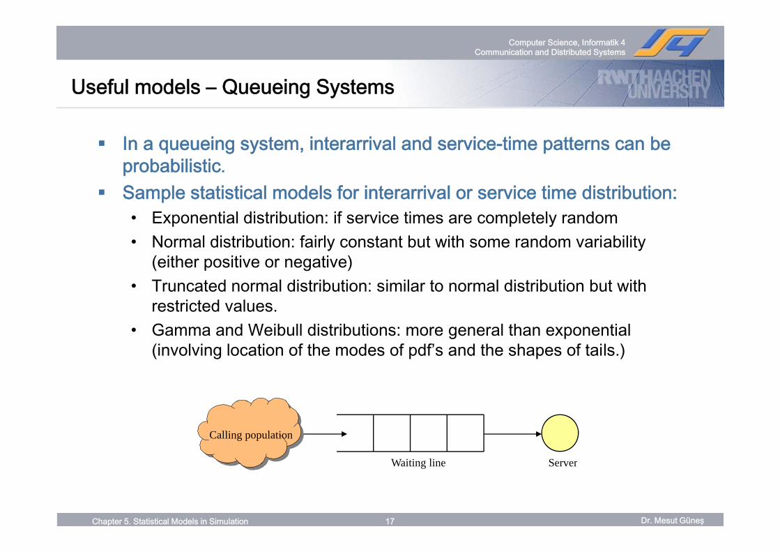
In a queueing system, interarrival and service-time patterns can be q g y , pprobabilistic.Sample statistical models for interarrival or service time distribution:

E ti l di t ib ti if i ti l t l d• Exponential distribution: if service times are completely random• Normal distribution: fairly constant but with some random variability

(either positive or negative)• Truncated normal distribution: similar to normal distribution but with

restricted values.• Gamma and Weibull distributions: more general than exponential g p

(involving location of the modes of pdf’s and the shapes of tails.)

ServerWaiting line

Calling population


ServerWaiting line


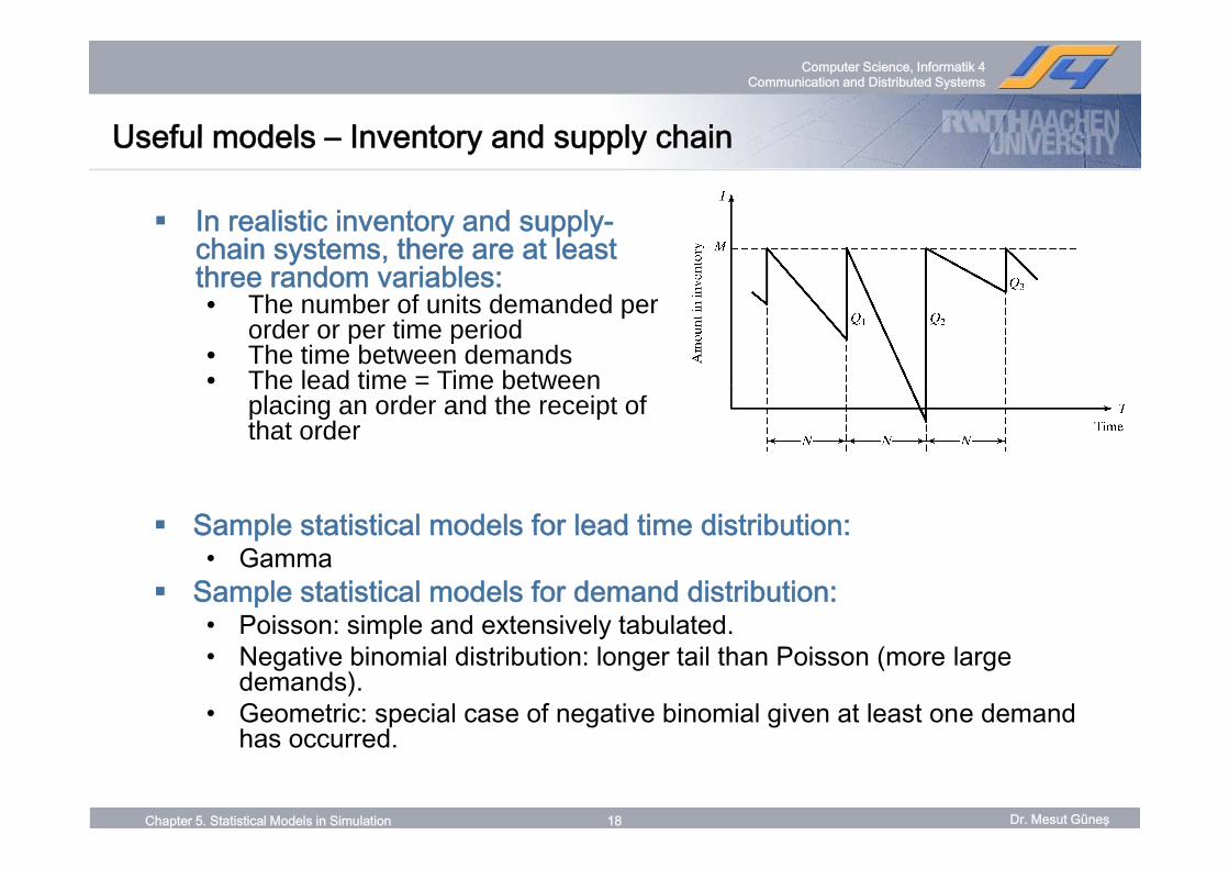
Useful models – Inventory and supply chainUseful models – Inventory and supply chain

In realistic inventory and supply-chain systems, there are at least three random variables:• The number of units demanded per

order or per time periodorder or per time period• The time between demands• The lead time = Time between

placing an order and the receipt of that order

Sample statistical models for lead time distribution:

that order

Sample statistical models for lead time distribution:• Gamma

Sample statistical models for demand distribution: • Poisson: simple and extensively tabulated.Poisson: simple and extensively tabulated.• Negative binomial distribution: longer tail than Poisson (more large

demands).• Geometric: special case of negative binomial given at least one demand

h d


has occurred.


Useful models – Reliability and maintainabilityUseful models – Reliability and maintainability

Time to failure (TTF)Time to failure (TTF)• Exponential: failures are random• Gamma: for standby redundancy where each component has an

exponential TTF• Weibull: failure is due to the most serious of a large number of

defects in a system of componentsdefects in a system of components• Normal: failures are due to wear



Useful models – Other areasUseful models – Other areas

For cases with limited data, some useful distributions are:For cases with limited data, some useful distributions are:• Uniform• Triangular• Beta

O h di ib iOther distribution: • Bernoulli• Binomial• Binomial• Hyperexponential



Discrete DistributionsDiscrete Distributions



Discrete DistributionsDiscrete Distributions

Discrete random variables are used to describe randomDiscrete random variables are used to describe random phenomena in which only integer values can occur.In this section, we will learn about:• Bernoulli trials and Bernoulli distribution• Binomial distribution

G t i d ti bi i l di t ib ti• Geometric and negative binomial distribution• Poisson distribution



Bernoulli Trials and Bernoulli DistributionBernoulli Trials and Bernoulli Distribution

Bernoulli Trials: • Consider an experiment consisting of n trials, each can be a success or

a failure.- Xj = 1 if the j-th experiment is a successj j p- Xj = 0 if the j-th experiment is a failure

failure success

• The Bernoulli distribution (one trial):

xp j 211,

)()( ⎨⎧ =

• where E(Xj) = p and V(Xj) = p(1-p) = pq

njxpq

pxpxp

j

jjjj ,...,2,1 ,

0,1:,

)()( =⎩⎨⎧

=−===


( j) p ( j) p( p) pq


Bernoulli Trials and Bernoulli DistributionBernoulli Trials and Bernoulli Distribution

Bernoulli process: p• n Bernoulli trials where trials are independent:

p(x1,x2,…, xn) = p1(x1)p2(x2) … pn(xn)



Binomial DistributionBinomial Distribution

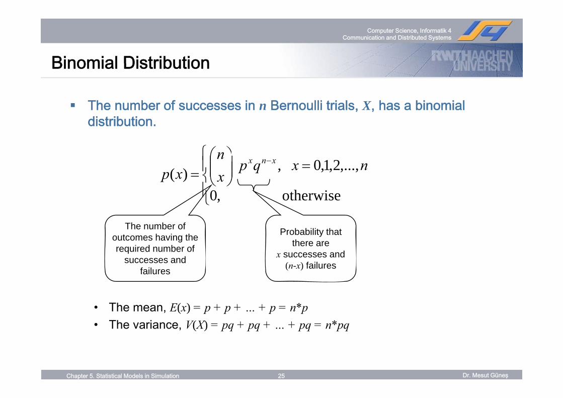
The number of successes in n Bernoulli trials, X, has a binomialThe number of successes in n Bernoulli trials, X, has a binomial distribution.

⎧ ⎞⎛n

⎪⎩

⎪⎨⎧

=⎟⎟⎠

⎞⎜⎜⎝

⎛=

−

otherwise,0

,...,2,1,0 , )( nxqpxn

xpxnx

The number of outcomes having the Probability that

there are

⎩ otherwise ,0

required number of successes and

failures

there are x successes and

(n-x) failures

• The mean, E(x) = p + p + … + p = n*p• The variance, V(X) = pq + pq + … + pq = n*pq



Geometric DistributionGeometric Distribution

Geometric distributionGeometric distribution• The number of Bernoulli trials, X, to achieve the 1st success:

⎩⎨⎧ =

=−

otherwise ,0,...,2,1,0 ,

)(1 nxpq

xpx

• E(x) = 1/p and V(X) = q/p2

⎩

E(x) 1/p, and V(X) q/p



Negative Binomial DistributionNegative Binomial Distribution

Negative binomial distributionNegative binomial distribution• The number of Bernoulli trials, X, until the k-th success • If Y is a negative binomial distribution with parameters p and k,

then:

⎪⎧

++=⎟⎟⎞

⎜⎜⎛ − − 21

1kkkypq

y kky

⎪⎩

⎪⎨

++=⎟⎟⎠

⎜⎜⎝ −=

otherwise ,0

,...2,1, , 1)( kkkypq

kxp

⎩

{successth

1 11

)(−

−− ⋅⎟⎟⎠

⎞⎜⎜⎝

⎛−−

=k

kky ppqky

xp31

• E(Y) = k/p, and V(X) = kq/p2

successes 1 )(k-44 344 21



Poisson DistributionPoisson Distribution

Poisson distribution describes many random processes quite well y p qand is mathematically quite simple.• where α > 0, pdf and cdf are:

⎧ x

⎪⎩

⎪⎨⎧

==−

otherwise ,0

,...1,0 ,!)( xe

xxpx

αα∑

=

−

=x

i

i

iexF

0 !)(

αα

• E(X) = α = V(X)⎩



Poisson DistributionPoisson Distribution

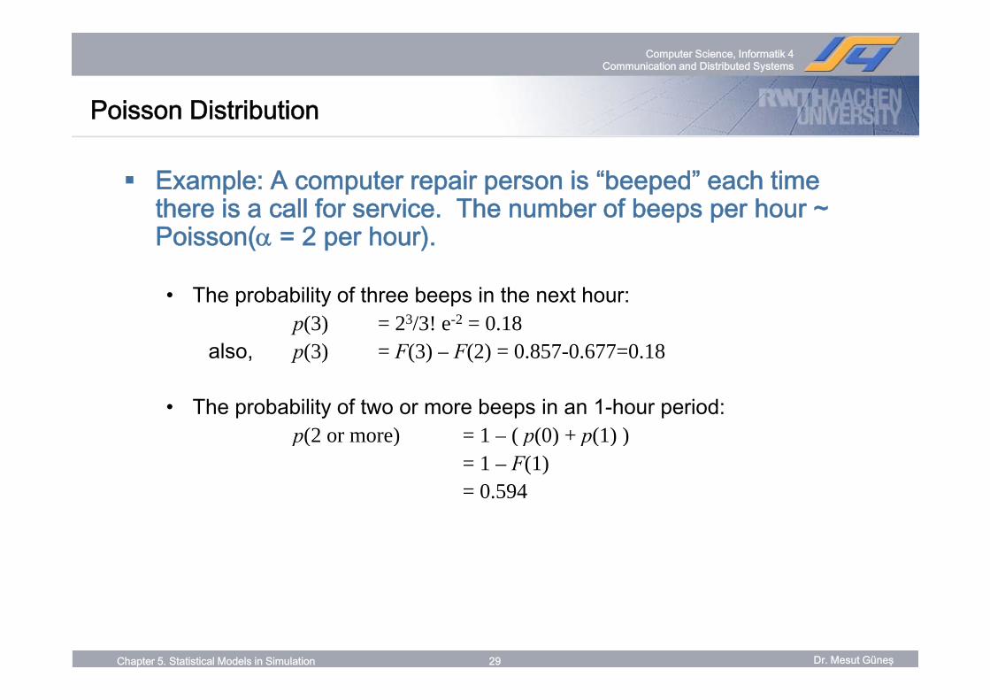
Example: A computer repair person is “beeped” each time p p p p pthere is a call for service. The number of beeps per hour ~ Poisson(α = 2 per hour).

• The probability of three beeps in the next hour:p(3) = 23/3! e-2 = 0.18

also p(3) = F(3) F(2) = 0 857 0 677=0 18also, p(3) = F(3) – F(2) = 0.857-0.677=0.18

• The probability of two or more beeps in an 1-hour period:(2 ) 1 ( (0) + (1) )p(2 or more) = 1 – ( p(0) + p(1) )

= 1 – F(1) = 0.594



Continuous DistributionsContinuous Distributions



Continuous DistributionsContinuous Distributions

Continuous random variables can be used to describeContinuous random variables can be used to describe random phenomena in which the variable can take on any value in some interval.

In this section, the distributions studied are:U if• Uniform

• Exponential• WeibullWeibull• Normal• Lognormal



Uniform DistributionUniform Distribution

A random variable X is uniformly distributed on the intervalA random variable X is uniformly distributed on the interval(a, b), U(a, b), if its pdf and cdf are:

⎪⎧ 1 ⎪⎧ < ax ,0

⎪⎩

⎪⎨⎧ ≤≤

−=otherwise ,0

,1)( bxa

abxf⎪⎩

⎪⎨

⎧

≥

<≤−−

=

bx

bxaabaxxF

,1

,

,

)(

Properties• P(x1 < X < x2) is proportional to the length of the interval

[F(x ) – F(x ) = (x -x )/(b-a)]

⎩ ,

[F(x2) F(x1) (x2-x1)/(b-a)]• E(X) = (a+b)/2 V(X) = (b-a)2/12

U(0,1) provides the means to generate random numbers, from which random variates can be


c a do a a es ca begenerated.


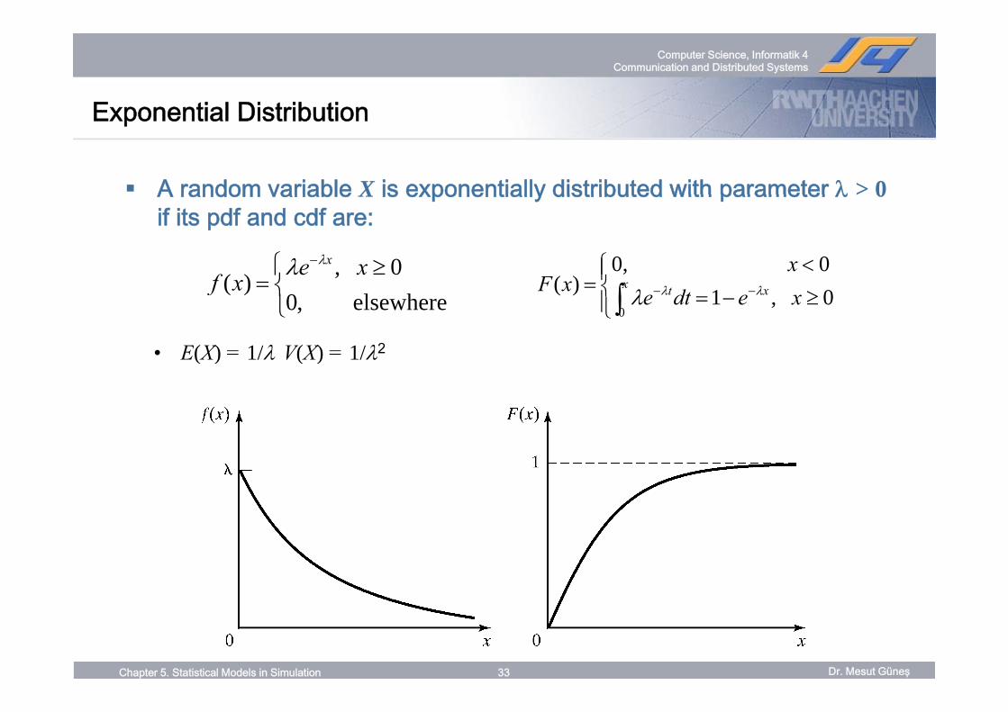
Exponential DistributionExponential Distribution

A random variable X is exponentially distributed with parameter λ > 0A random variable X is exponentially distributed with parameter λ > 0if its pdf and cdf are:

⎨⎧ ≥− 0 ,

)(xe

fxλλ ⎪

⎨⎧ < 0 0, x

⎩⎨=

elsewhere ,0,

)(xf⎪⎩

⎪⎨ ≥−=

=∫ −− 0 ,1)(0

xedtexF x xt λλλ

• E(X) = 1/λ V(X) = 1/λ2E(X) 1/λ V(X) 1/λ




• Used to model interarrival times when arrivals are completely random, and to model service times that are highly variable

• For several differentFor several different exponential pdf’s (see figure), the value of intercept on the vertical axis is λ, and all pdf’s e t ca a s s λ, a d a pd seventually intersect.




Memoryless property• For all s and t greater or equal to 0:

P(X > s+t | X > s) = P(X > t)

• Example: A lamp ~ exp(λ = 1/3 per hour), hence, on average, 1 failure per 3 hours.

- The probability that the lamp lasts longer than its mean life is:P(X > 3) = 1 – (1 – e -3/3) = e -1 = 0.368

Th b bilit th t th l l t b t 2 t 3 h i- The probability that the lamp lasts between 2 to 3 hours is:P(2 <= X <= 3) = F(3) – F(2) = 0.145

The probability that it lasts for another hour given it is operating for- The probability that it lasts for another hour given it is operating for 2.5 hours:

P(X > 3.5 | X > 2.5) = P(X > 1) = e -1/3 = 0.717




Memoryless propertyy p p y

)()|( tsXPsXtsXP +>=>+>

)()|(

)(esXP

sXtsXP

ts

>=>+>

+−λ

ee

t

s

=

=

−

−

λ

λ

)( tXPe

>=



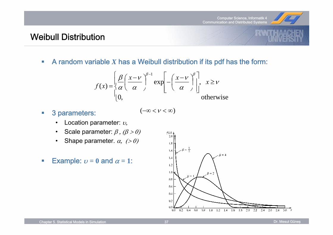
Weibull DistributionWeibull Distribution

A random variable X has a Weibull distribution if its pdf has the form:a do a ab e as a e bu d st but o ts pd as t e o

⎪

⎪⎨

⎧≥

⎥⎥⎦

⎤

⎢⎢⎣

⎡⎟⎠⎞

⎜⎝⎛ −

−⎟⎠⎞

⎜⎝⎛ −

=

−

,exp)(

1

να

να

ναβ ββ

xxxxf

3 parameters:

⎪⎩

⎥⎦⎢⎣ ⎠⎝⎠⎝otherwise ,0

)( ∞<<−∞ ν

• Location parameter: υ, • Scale parameter: β , (β > 0)• Shape parameter. α, (> 0)( )

Example: υ = 0 and α = 1:



Weibull DistributionWeibull Distribution

Weibull Distribution

⎪

⎪⎨

⎧≥

⎥⎥⎦

⎤

⎢⎢⎣

⎡⎟⎠⎞

⎜⎝⎛ −

−⎟⎠⎞

⎜⎝⎛ −

=

−

,exp)(

1

να

να

ναβ ββ

xxxxf

For β = 1, υ=0

⎪⎩

⎦⎣otherwise ,0

⎪⎩

⎪⎨⎧

≥=−

other ise0

,exp1)(

1

να

α xxfx

⎪⎩ otherwise ,0

When β = 1, (λ / )


X ~ exp(λ = 1/α)


Normal DistributionNormal Distribution

A random variable X is normally distributed if it has the pdf:A random variable X is normally distributed if it has the pdf:

∞<<∞−⎥⎥⎦

⎤

⎢⎢⎣

⎡⎟⎠⎞

⎜⎝⎛ −

−= xxxf ,21exp

21)(

2

σμ

πσ

• Mean:

⎥⎦⎢⎣ ⎠⎝22 σπσ

∞<<∞− μ02• Variance:

• Denoted as X ~ N(μ,σ2)02 >σ

Special properties:• 0)(lim and ,0)(lim ==

∞→−∞→xfxf

xx

• f(μ-x)=f(μ+x); the pdf is symmetric about μ.• The maximum value of the pdf occurs at x = μ; the mean and mode are

equal.




Evaluating the distribution:Evaluating the distribution:• Use numerical methods (no closed form)• Independent of μ and σ, using the standard normal distribution:

Z ~ N(0,1)• Transformation of variables: let Z = (X - μ) / σ,

⎞⎛( )

1

)(

/)(

σμ

⎟⎠⎞

⎜⎝⎛ −

≤=≤=xZPxXPxF

1

21

/)(

/)( 2/2

σμ

σμ

π−

−

∞−

−=

∫

∫x

x z dze

∫ ∞−

−=Φz t dtez 2/2

21)( where,π

)()(/)(

σμσμ

φ −

∞−Φ== ∫ xx

dzz




Example: The time required to load an oceangoing vessel, X, isExample: The time required to load an oceangoing vessel, X, is distributed as N(12,4), µ=12, σ=2• The probability that the vessel is loaded in less than 10 hours:

1587.0)1(2

1210)10( =−Φ=⎟⎠⎞

⎜⎝⎛ −

Φ=F

- Using the symmetry property, Φ(1) is the complement of Φ (-1)



Lognormal DistributionLognormal Distribution

A random variable X has a lognormal distribution if its pdf has theA random variable X has a lognormal distribution if its pdf has the form:

( )⎪⎧

>⎥⎤

⎢⎡ −− 0lnexp1 2

xμx1

• Mean E(X) = e μ+σ2/2

⎪⎩

⎪⎨

>⎥⎦

⎢⎣=

otherwise 0,

0 ,2

exp2)( 2 x

σσxπxf μ=1, σ2=0.5,1,2.

Mean E(X) e μ

• Variance V(X) = e 2μ+σ2/2 (eσ2 - 1)

Relationship with normal distribution• When Y N(μ σ2) then X = eY lognormal(μ σ2)• When Y ~ N(μ, σ2), then X = eY ~ lognormal(μ, σ2)• Parameters μ and σ2 are not the mean and variance of the lognormal

random variable X



Poisson ProcessPoisson Process




Definition: N(t) is a counting function that represents the number ( ) g pof events occurred in [0,t].

A counting process {N(t) t>=0} is a Poisson process with meanA counting process {N(t), t>=0} is a Poisson process with mean rate λ if:• Arrivals occur one at a time

{N(t) t> 0} has stationary increments• {N(t), t>=0} has stationary increments- Number of arrivals in [t, t+s] depends only on s, not on starting point t- Arrivals are completely random

• {N(t), t>=0} has independent increments- Number of arrivals during nonoverlapping time intervals are independent

Future arrivals occur completely random- Future arrivals occur completely random




Propertiesp

( ) ,...2,1,0 and 0for ,!)()( =≥== − nte

ntntNP t

nλλ

• Equal mean and variance: E[N(t)] = V[N(t)] = λ t

St ti i t• Stationary increment:- The number of arrivals in time s to t, with s<t, is also Poisson-

distributed with mean λ(t-s)



Poisson Process – Interarrival TimesPoisson Process – Interarrival Times

Consider the interarrival times of a Possion process (A1, A2, …), where Ai is p ( 1, 2, ), ithe elapsed time between arrival i and arrival i+1

• The 1st arrival occurs after time t iff there are no arrivals in the interval [0, t],The 1 arrival occurs after time t iff there are no arrivals in the interval [0, t], hence:

P(A1 > t) = P(N(t) = 0) = e-λt

P(A1 <= t) = 1 – e-λt [cdf of exp(λ)]

• Interarrival times, A1, A2, …, are exponentially distributed and independent with mean 1/λmean 1/λ

Arrival counts ~ Poisson(λ)

Interarrival time ~ Exp(1/λ)


Stationary & Independent Memoryless


Poisson Process – Splitting and PoolingPoisson Process – Splitting and Pooling

Splitting:p g• Suppose each event of a Poisson process can be classified as Type I,

with probability p and Type II, with probability 1-p.

• N(t) = N1(t) + N2(t), where N1(t) and N2(t) are both Poisson processes with rates λp and λ(1-p)

N1(t) ~ Poisson[λp]λpN(t) ~ Poisson(λ)

N1(t) Poisson[λp]

N2(t) ~ Poisson[λ(1-p)]

λλp

λ(1-p)



Poisson Process – Splitting and PoolingPoisson Process – Splitting and Pooling

Pooling:n

jnNPjNPnNNP )()()( 2121 −====+ ∑Pooling:• Suppose two Poisson

processes are pooled together• N1(t) + N2(t) N(t) where N(t)

n

j

tjn

tj

j

ejn

tejt

)!()(

!)(

0

21

0

21λλ λλ

−= −

−−

=

∑

∑

• N1(t) + N2(t) = N(t), where N(t)is a Poisson processes with rates λ1 + λ2

n

j

jnjtt

j

jnt

jtee

jnj

)!()(

!)(

)!(!

0

21

0

21λλλλ

−=

=

−−−

=

∑n

j

jnjnt

j

jnjte

jj

)!(!

)(

0

21)(

0

21λλλλ

−=

=

−+− ∑

N1(t) ~ Poisson[λ1] N2(t) ~ Poisson[λ2]n

j

jnjnt

jnjn

nte

)!(!!

! 0

21)( 21λλλλ

−=

=

−+− ∑

λ λ

λ1 λ2

n

n

j

jnjn

t

jn

nte

! 021

)( 21 λλλλ⎟⎟⎠

⎞⎜⎜⎝

⎛=

=

−+− ∑N(t) ~ Poisson(λ1 + λ2)

λ1 + λ2


nn

t

nte )(

! 21)( 21 λλλλ += +−


Empirical DistributionsEmpirical Distributions



Empirical Distributions

A distribution whose parameters are the observed values in a sample

Empirical Distributions

A distribution whose parameters are the observed values in a sample of data.• May be used when it is impossible or unnecessary to establish that a

random variable has any particular parametric distributionrandom variable has any particular parametric distribution.• Advantage: no assumption beyond the observed values in the sample.• Disadvantage: sample might not cover the entire range of possible values.



Empirical Distributions - ExampleEmpirical Distributions - Example

Customers arrive in groups from 1 to 8 personsCustomers arrive in groups from 1 to 8 personsObservation of the last 300 groups has been reportedSummary in the table belowy

Group Frequency Relative Cumulative RelativeGroupSize

Frequency Relative Frequency

Cumulative Relative Frequency

1 30 0.10 0.102 110 0 37 0 472 110 0.37 0.473 45 0.15 0.624 71 0.24 0.865 12 0 04 0 905 12 0.04 0.906 13 0.04 0.947 7 0.02 0.96


8 12 0.04 1.00


Empirical Distributions - ExampleEmpirical Distributions - Example



Summary

The world that the simulation analyst sees is probabilistic, not

Summary

The world that the simulation analyst sees is probabilistic, not deterministic.In this chapter:• Reviewed several important probability distributions.• Showed applications of the probability distributions in a simulation context.

Important task in simulation modeling is the collection and analysis ofImportant task in simulation modeling is the collection and analysis of input data, e.g., hypothesize a distributional form for the input data. Student should know:

Diff b t di t ti d i i l di t ib ti• Difference between discrete, continuous, and empirical distributions.• Poisson process and its properties.



Poisson Process – Nonstationary Poisson ProcessPoisson Process – Nonstationary Poisson Process

Poisson Process without the stationary increments, characterized by λ(t), the o sso ocess t out t e stat o a y c e e ts, c a acte ed by λ(t), t earrival rate at time t.The expected number of arrivals by time t, Λ(t):

∫t

∫=tλ(s)dsΛ(t)

0

Relating stationary Poisson process n(t) with rate λ=1 and NSPP N(t) with rate λ(t):• Let arrival times of a stationary process with rate λ = 1 be t1, t2, …, and 1 2

arrival times of a NSPP with rate λ(t) be T1, T2, …, we know:

ti = Λ(Ti)ti Λ(Ti)Ti = Λ−1(ti)



Poisson Distribution – Nonstationary Poisson Process

Example: Suppose arrivals to a Post Office have rates 2 per minute from 8 am

Poisson Distribution – Nonstationary Poisson Process

p pp puntil 12 pm, and then 0.5 per minute until 4 pm. Let t = 0 correspond to 8 am, NSPP N(t) has rate function:

⎧ <≤ 402 t

Expected number of arrivals by time t:⎩⎨⎧

<≤<≤

=84 ,5.040 ,2

)(tt

tλ

Expected number of arrivals by time t:

⎪

⎪⎨⎧

<≤+=+

<≤=Λ

∫ ∫ 846502

40 ,2)( 4

ttdsds

ttt t

Hence, the probability distribution of the number of arrivals between 11 am and 2 pm

⎪⎩<≤+=+∫ ∫ 84 ,6

25.02

0 4tdsds

and 2 pm.P[N(6) – N(3) = k] = P[N(Λ(6)) – N(Λ(3)) = k]

= P[N(9) – N(6) = k]= e(9-6)(9-6)k/k! = e3(3)k/k!


e( )(9-6) /k! e (3) /k!

05 statistical models in simulation.ppt … · computer science, informatik 4 communication and...

Documents