General Aeroacoustic Environment Basics and Wind Tunnel Testing and Analysis Topics

Darren K. ReedAerosciences Branch

Marshall Space Flight Center16 N b 201116 November 2011

Outline

♦ Aeroacoustic Environment Goals

♦ Basic Definitions

♦ Vehicle Development Phases♦ Vehicle Development Phases

♦ Vehicle Acoustic Zone Definition & Examples

♦ Preliminary Environment Development

♦ Final Environment Developmentp

• Trajectory Analyses

• Wind Tunnel Test Matrix Development & Examples

• Recent Aeroacoustic Models

• Instrumentation

• Data Acquisition

• Data Processing

• Data Scaling• Data Scaling

• Time Durations

♦ Flight Instrumentation

2

External Launch Vehicle Acoustic Environments

♦ Launch vehicles experience very high level noise levels during liftoff, ascent, and possible reentry

♦ Liftoff acoustic environments are due to supersonic plume interaction with the♦ Liftoff acoustic environments are due to supersonic plume interaction with the exhaust deflector and launch pad/platform

♦ Ascent aeroacoustics is due to the turbulence in the boundary layer

♦ Separation motor noise – short term, localized plume noise source

♦ Reentry noise levels are highly dependent on the trajectory:  Orbiter reentry noise was lower than ascent, but the SRB noise levels were extremely high

♦ This presentation will concentrate on ascent aeroacoustics, however, liftoff noise♦ This presentation will concentrate on ascent aeroacoustics, however, liftoff noise levels could be the dominate source at particular zones

3

Basic Goals for Aeroacoustic Environments

♦ Develop aeroacoustic environments that conservatively describe the flight environment

♦ Provide the vibroacoustic analysts environments that can be used to develop the♦ Provide the vibroacoustic analysts environments that can be used to develop the vibroacoustic criteria

E i i l E ti & D tEmpirical Equations & Data scaled from other vehicles

Wind Tunnel Tests Derived Environments Vibroacoustic Team

Flight Data

4

Aeroacoustic Environments

♦ What are the aeroacoustic environments?

• The noise generated by turbulence within the boundary layer

• The levels are highly dependent on the outer mold line and flow dynamic pressure• The levels are highly dependent on the outer mold line and flow dynamic pressure

• Generally, the environments are defined by a spectrum, usually a 1/3 octave constant percentage band spectra and an applied time duration

• This information is used by the vibroacoustics groups to define the vibration criteria for major structures and attached components

♦ The vibration criteria are used to help design and for qualification tests for the componentscomponents

• Most major structures are “sized” for loads and stress – vibration is usually a smaller influence

5

Progression of Environments

♦ Phase A (or earlier) = Preliminary Environments

• Start identifying the acoustic zones

• Rough order of magnitude• Rough order of magnitude

• Use empirical equations or scale data from other applicable vehicle tests or flights

• Data scaled using preliminary nominal trajectories (3DOF)

♦ Prior to Critical Design Review = Final Environments

• Better definition of acoustic zones and protuberance zones

• Environments are generally developed from sub‐scale model wind tunnel tests

• Wind tunnel test instrumentation is highly correlated with zones

• Data scaled with latest launch vehicle dispersed trajectories (6DOF)

♦ Flight Data Updated environments♦ Flight Data – Updated environments

• Flight instrumentation used to validate final environments where available

6

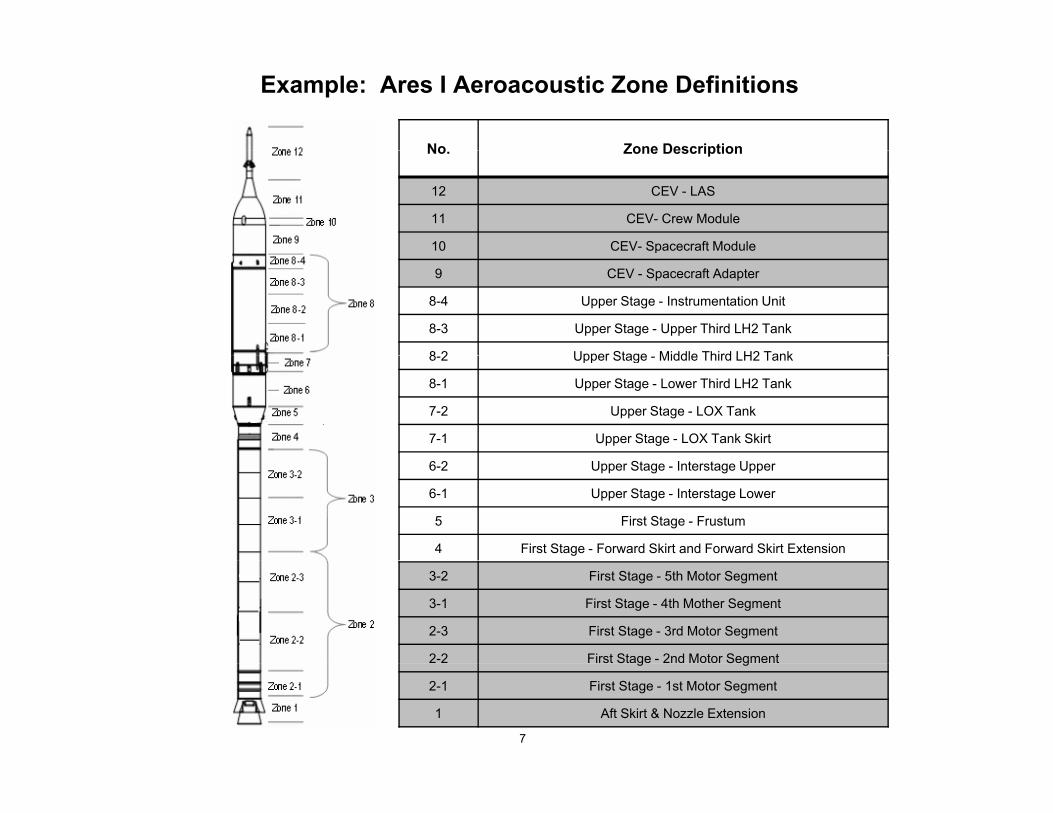
Example: Ares I Aeroacoustic Zone Definitions

No Zone DescriptionNo. Zone Description

12 CEV - LAS

11 CEV- Crew Module

10 CEV- Spacecraft Modulep

9 CEV - Spacecraft Adapter

8-4 Upper Stage - Instrumentation Unit

8-3 Upper Stage - Upper Third LH2 Tank

8 2 Upper Stage Middle Third LH2 Tank8-2 Upper Stage - Middle Third LH2 Tank

8-1 Upper Stage - Lower Third LH2 Tank

7-2 Upper Stage - LOX Tank

7-1 Upper Stage - LOX Tank Skirt

6-2 Upper Stage - Interstage Upper

6-1 Upper Stage - Interstage Lower

5 First Stage - Frustum

4 First Stage - Forward Skirt and Forward Skirt Extension

3-2 First Stage - 5th Motor Segment

3-1 First Stage - 4th Mother Segment

2-3 First Stage - 3rd Motor Segment

2-2 First Stage - 2nd Motor Segment

7

S g S g

2-1 First Stage - 1st Motor Segment

1 Aft Skirt & Nozzle Extension

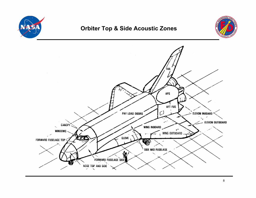
Orbiter Top & Side Acoustic Zones

8

Preliminary Environment Development

Estimate Flow Conditions for Each Zone for Subsonic, Transonic, and Supersonic Conditions

Attached Turbulent Boundary Layer (ATBL) – lowest levels

Compression separated flow – mid to high levels

Expansion separated flow – mid to high levelsp p g

Shock induced separated flow – high levels

Protuberances experience a mix of the above flow fields

Zone 1 Zone 2 Zone 3 Zone 4 Zone 5 Zone 6

Example of flow types chosen for different zonesZone 1 Zone 2 Zone 3 Zone 4 Zone 5 Zone 6

Subsonic ATBL ATBL ATBL ATBL ATBL ATBL

Transonic Compression Expansion ATBL ATBL ATBL Expansion

9

Supersonic Compression ATBL ATBL ATBL ATBL Expansion

Preliminary Environment Development

Subsonic Transonic Supersonic

Flow Fields for Basic Vehicle Configurations

10

Fluctuating Pressure Levels for Different Flow Fields(not necessarily in the same zone)

170

als)

ATBL

Transonic Compression Plateau

T i C i P k

160

20m

icro

Pasc

a Transonic Compression PeakTransonic Expansion

Supersonic Compression PlateauSupersonic Compression Peak

150

Leve

l, dB

(re.

130

140

ting

Pres

sure

120

130

0 5 1 0 1 5 2 0 2 5 3 0 3 5 4 0

Fluc

tuat

11

0.5 1.0 1.5 2.0 2.5 3.0 3.5 4.0Mach Number

Empirically Derived Spectra

12

Preliminary Environment Development

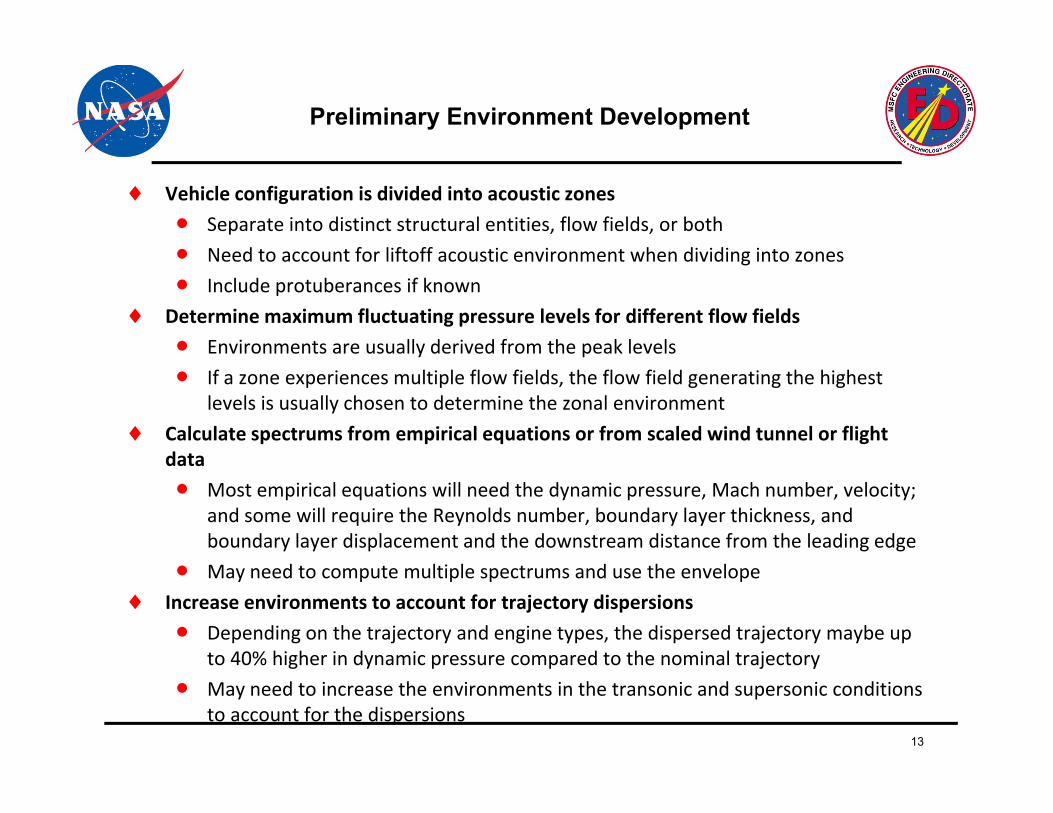
♦ Vehicle configuration is divided into acoustic zones

• Separate into distinct structural entities, flow fields, or both

• Need to account for liftoff acoustic environment when dividing into zones• Need to account for liftoff acoustic environment when dividing into zones

• Include protuberances if known

♦ Determine maximum fluctuating pressure levels for different flow fields

• Environments are usually derived from the peak levelsy p

• If a zone experiences multiple flow fields, the flow field generating the highest levels is usually chosen to determine the zonal environment

♦ Calculate spectrums from empirical equations or from scaled wind tunnel or flight datadata

• Most empirical equations will need the dynamic pressure, Mach number, velocity; and some will require the Reynolds number, boundary layer thickness, and boundary layer displacement and the downstream distance from the leading edge

• May need to compute multiple spectrums and use the envelope

♦ Increase environments to account for trajectory dispersions

• Depending on the trajectory and engine types, the dispersed trajectory maybe up to 40% higher in dynamic pressure compared to the nominal trajectoryto 40% higher in dynamic pressure compared to the nominal trajectory

• May need to increase the environments in the transonic and supersonic conditions to account for the dispersions

13

Final Environment Development

♦ To assure the best quality aeroacoustic environment, NASA has always used dedicated wind tunnel tests for manned vehicles

♦ Analysis of the trajectory data is needed for scaling and test matrix development♦ Analysis of the trajectory data is needed for scaling and test matrix development

♦ The timing of the tests are a balance of when acceptable moldlines are available and when the vibroacoustic group requires the environment – usually prior to CDR

♦ Wind Tunnel Testing

• The selection of the wind tunnel facility, the model size, number of instruments, range of velocities, and vehicle attitudes must be balanced with the available funds

• Only a few wind tunnels that can handle 1% to 4% subscale models with launch yvehicle type flow conditions

• Instrumentation is fragile and expensive

• Data acquisition systems must be capable of very high sample rates

• Al d k i h i i• Always cost more and takes more time than you can imagine

♦ Post‐test analyses

• Even with the best automation, the process is slow and tedious

♦ Databook results are to verify the preliminary environments, but usually just replaces♦ Databook results are to verify the preliminary environments, but usually just replaces the preliminary environments

14

Trajectory Analysis for Wind Tunnel Data Scaling

♦ Trajectory analyses predicts the vehicle attitude, position, velocity, and many other parameters

♦ The most important parameters for aeroacoustics are: Mach number dynamic♦ The most important parameters for aeroacoustics are: Mach number, dynamic pressure, angle‐of‐attack, sideslip, static temperature, density, Reynolds number

♦ Most G&NC software suites can provide hundreds of parameters

♦ The first trajectory requirement is the Mach, angle‐of‐attack ,and sideslip ranges

• This data is used to setup the run matrix in terms of the vehicle attitude range

♦ The static temperature is used to frequency (Strouhal) scale the data

♦ Dynamic pressure levels are used to directly scale the fluctuating pressure levels

♦ A six degree of freedomMonte Carlo dispersed trajectory set is generally used to♦ A six degree of freedom Monte Carlo dispersed trajectory set is generally used to develop the environments

• Typically get a set of two thousand or more trajectories

• Statistics are computed for dynamic pressure, angle‐of‐attack, and sideslip angle

• MSFC has typically used the one‐sided tolerance limit of a probability of 97.5% with a confidence of 50% for the SRB reentry and the initial Ares I assessments

15

Trajectory Analysis for Wind Tunnel Data Scaling cont.

♦ 1 of 8 trajectory sets for this version♦This is a “light-fast” trajectory: i.e. lower mass launched in summer (higher performance)♦Red triangles show the♦Red triangles show the P95/C50 levels

16

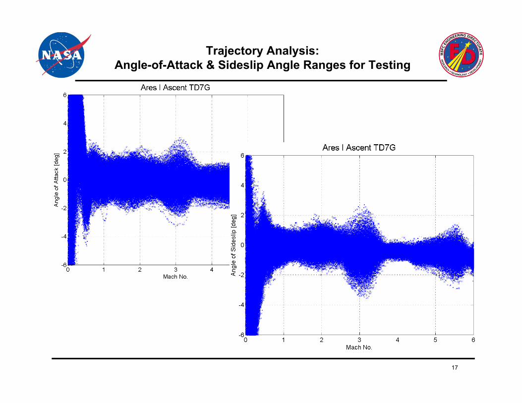
Trajectory Analysis: Angle-of-Attack & Sideslip Angle Ranges for Testing

17

Test Matrix Development

♦ The test matrix shows what runs are needed, but not the schedule

♦ The test matrix shows the following conditions:

• Flow velocity Mach number; Reynolds No• Flow velocity – Mach number; Reynolds No.

• Vehicle attitude (angle‐of‐attack & sideslip or total angle‐of‐attack & roll angle)

• Vehicle configuration (boosters on & off, control surface deflections, different payload fairings, etc.)

• Type of runs (sweeps, pitch pause, flow visualization, specific instrumentation runs….)

• Run priority

• Shock Reflection either avoid these conditions or toss affected measurements• Shock Reflection – either avoid these conditions or toss affected measurements

♦ The total number of runs will be a balance between available funding and the requirements

♦ The run schedule is a balance between tunnel efficiency ($), and run priorities

• Should run the highest priority runs first, but tunnel operating efficiencies will work against the priority list

♦ Run priority is based on users judgment of the aeroacoustic environment

• Transonic conditions usually produce higher levels than subsonic or high• Transonic conditions usually produce higher levels than subsonic or high supersonic, therefore are usually the highest priority

18

Test Matrix : Ares I Ascent Aeroacoustic Testing

α, deg Φ , deg 0.50 0.60 0.80 0.85 0.90 0.95 1.05 1.10 1.20 1.40 Max 1.55 1.75 2.00 2.25 2.50 Runs Points3 3 2 1 1 1 1 1 2 2 2 2 1 3 4 5

0 0 3.0 m-swp 2 80 1A1 0 3.0 p-p β=0 0 0 0 0 0 0 0 0 0 0 0 0 0 0 0 16 240 1A2 0 3 0 0 0 0 0 0 0 0 0 0 0 0 0 0 0 0 0 16 240 1

ΔM = 0.025 @ β=0

Totals9' x 7' SWTAttitude Schedulepriority

priority>>>

Config Re/ft x 10-6 Type

ΔM = 0.025 @ β=0

11' x 11' TWT

A2 0 3.0 p-p 0 0 0 0 0 0 0 0 0 0 0 0 0 0 0 0 16 240 1A1 0 5.0 p-p 0 0 0 0 0 0 0 0 0 0 0 0 0 0 0 0* 16 240 10 0 3.0 p-p B1 B1 B1 B1 B1 B1 B1 B1 B1 B1 B1 B3 B1 B1 B1 B1 16 232 11 0 3.0 p-p B1 B1 B1 B1 B1 B1 B1 B1 B1 B1 B1 B3 B1 B1 B1 B1 16 232 1-1 0 3.0 p-p B1 B1 B1 B1 B1 B1 B1 B1 B1 B1 B1 B3 B1 B1 B1 B1 16 232 12 0 3.0 p-p B1 B1 B1 B1 B1 B1 B1 B1 B1 B1 B1 B3 B1 B1 B1 B1 16 232 1-2 0 3.0 p-p B1 B1 B1 B1 B1 B1 B1 B1 B1 B1 B1 B3 B1 B1 B1 B1 16 232 13 0 3 0 p p B2 B2 B2 B2 B2 B2 B2 B2 B2 B2 B2 B4 B2 B2 B2 B2 16 140 2ub

eren

ces

3 0 3.0 p-p B2 B2 B2 B2 B2 B2 B2 B2 B2 B2 B2 B4 B2 B2 B2 B2 16 140 2-3 0 3.0 p-p B2 B2 B2 B2 B2 B2 B2 B2 B2 B2 B2 B4 B2 B2 B2 B2 16 140 25 0 3.0 p-p B2 B2 B2 B2 B2 B2 B2 B2 B2 B2 B2 B4 B2 B2 B2 B2 16 140 2-5 0 3.0 p-p B2 B2 B2 B2 B2 B2 B2 B2 B2 B2 B2 B4 B2 B2 B2 B2 16 140 27 0 3.0 p-p B2 B2 B2 B2 B2 B2 B2 B2 B2 B2 B2 B4 B2 B2 B2 B2 16 140 2-7 0 3.0 p-p B2 B2 B2 B2 B2 B2 B2 B2 B2 B2 B2 B4 B2 B2 B2 B2 16 140 20 90 3.0 p-p B2 1 9 31 90 3 0 p p B2 1 9 3

Are

s I w

ith p

rotu

1 90 3.0 p-p B2 1 9 3-1 90 3.0 p-p B2 1 9 32 90 3.0 p-p B2 1 9 3-2 90 3.0 p-p B2 1 9 33 90 3.0 p-p B2 1 9 3-3 90 3.0 p-p B2 1 9 3

Repeat A1 0 3.0 p-p 0 0 0 0 0 0 0 0 0 0 0 0 0 0 0 0 16 240 1

Forward Shadowgraph

0 0 3.0 p-p B3 B1 B1 B1 B1 5 67 3

254 3,170*Max Re < 5-million

No.1515A2

A1 -7, -6, -5, -4, -3, -2, -1, 0, 1, 2, 3, 4, 5, 6, 77, 6, 5, 4, 3, 2, 1, 0, -1, -2, -3, -4, -5, -6, -7

Overall Totals

Attitude Schedules Positions, deg Shadowgraph in the 9x7 tunnel will require separate forward and aft optical setups to capture shock patterns at both ends.

19

15975B4 -3, -1, 0, 1, 3

B3 -3, -2, -1, 0, 1, 2, 3

B1-7, -5, -3, -1, 0, 1, 3, 5, 7B2

-7, -6, -5, -4, -3, -2, -1, 0, 1, 2, 3, 4, 5, 6, 7 Shadowgraph in the 11' tunnel will only need to be done once. Either the initial run or the repeat will suffice.

Shock Reflection on Ares I Model in ARC 9x7

20

Ares I Aeroacoustic Model in ARC 9x7 Supersonic WT

21

Ares I 2.8% First Stage Reentry Aeroacoustic WT Model

22

3%-scale STS model at ARC 9 x 7 Supersonic UPWT

23

Model Instrumentation (I)

♦ For aeroacoustics we generally use extremely small Kulite® fluctuating pressure transducers

• No other vendor can realistically compete (my opinion)

• EXTREMELY LONG LEAD TIME FOR DELIVERY; sometimes as much as 24 weeks;

♦ More measurements = better defined environments

• Typically assign vehicle zones and strive to have at least three measurements per zone

• Very difficult & expensive to repair/replace transducers during the test – therefore more “in‐situ” replacement xducers are desirablep

♦ Should have a plan & process of how the data will be used to develop the environment

• The type of data processing will influence the number of measurements and transducer placement

− May need more measurements if zonal averaging is usedy g g

♦ Kulites are very fragile & their performance is very dependent on the installment accuracy

♦ Amplifiers – desirable to have close to transducer

• Reduces “losses” especially at very high frequencies

• Minimizes extraneous electronic noise• Minimizes extraneous electronic noise

• Nice to have amplifiers “in” the model, but not required

• Helps with impedance matching between the transducer and data acquisition hardware

24

Fluctuating Pressure Transducer Model Placement

♦ For typical “rocket” moldlines, many put in rings at specific X‐stations

• May allow “zonal averaging” at the specific ring X‐station

♦ Nice also to have a specific clocking positionsp g p

♦ Need for transducers to surround and possibly on large protuberances

Orion tests put 4 to 8 transducers per ring at specific X-stations

Ares I tests mainly put measurements at specific clocking angles and the many protuberances (Kxxx –fluctuating, Pxxx –static pressures

25

Data Acquisition – High Sample Rate Rationale

WTWTFLT

FLT fDD

UUf ⎟⎟

⎠

⎞⎜⎜⎝

⎛⎟⎟⎠

⎞⎜⎜⎝

⎛=

Symbol Description

f Frequency

U Velocity

Ch t i ti l th

Strouhal scaling of frequency dictates very high sample rate

UfD

UfD

⎟⎠⎞

⎜⎝⎛=⎟

⎠⎞

⎜⎝⎛

FLTWT DU ⎟⎠

⎜⎝

⎟⎠

⎜⎝ D Characteristic length

M Mach number

a Speed of sound

T Static temperature (°R)WT

FLT

WT

WT

FLTFLT f

DD

MaMaf ⎟⎟

⎠

⎞⎜⎜⎝

⎛⎟⎟⎠

⎞⎜⎜⎝

⎛=

FLTWT UU ⎠⎝⎠⎝

)(0.49 RTa °≅

WTFLT MM =

( ) WTWT

FLTFLT f

TT

f %42 −⎟⎟⎠

⎞⎜⎜⎝

⎛=

Th f f ll l f f 2kHThus, for a full scale max frequency of 2kHz, the wind tunnel data acquisition sample rate is ~ 160ksps

Frequency scaling can change with Mach number – especially above Mach = 2 0number especially above Mach = 2.0

26

Data Acquisition Capability & Real-time Monitoring

♦ Most wind tunnels have high speed data acquisition systems, but few can handle large numbers of fluctuating pressure transducers at very high sample rates

♦ One of the more difficult issues is real‐time data monitoring during the test

• Need to insure data is being acquired accurately and all systems are working properly

• Some facilities have software to allow some real‐time data monitoring

• Rarely have the time, resources, or man‐power to completely check data during test

• MSFC typically requests full scale data based on a set dynamic pressure profile from a yp y q y p ptrajectory set, and a set frequency scaling (Strouhal)

− Easier for analysts to understand the environments in full scale in decibels

♦ Other data

• May gather static datay g

• Might request shadowgraph or Schlieren photos or videos during the test

• Sometimes request a set of triaxial accelerometer data to monitor model dynamics

− This is mainly to ensure model integrity and tunnel safety

27

Data Corrections

28

Data Corrections

♦ Most wind tunnels have noise generated by the drive/turbine that will have to be corrected (eliminated)

• Most tunnels have empty tunnel calibration studies that document these issues• Most tunnels have empty tunnel calibration studies that document these issues

♦ Most transonic wind tunnels have holes or slots in the test section to help reduce shock effects – these holes & slots can generate high noise peaks in the data

♦ Some transducer mounting methods will introduce a high frequency peak in the data h h ld b dthat should be corrected

• Highly dependent on each transducer mounting – seemingly identical transducer mounts can give different results (maybe a function of transducer compliance)

♦ Most of these corrections cannot be done automatically or in batchesy

• Effects of the above problems change with Mach number, model attitude, and model induced noise levels

• Fixing these problems is a very time consuming and tedious task

29

Post Test Processing

♦ Facility will provide data, usually on a portable hard drive

• Format of data is dependent on the facility, can be time domain or frequency domain and is usually developed and agreed upon early in the planningdomain and is usually developed and agreed upon early in the planning

♦ Need processes and/or software routines to eliminate bad data

• This can get very complex for very large number of transducers and/or run conditions

• Checks of the rms levels, Gaussian distributions, amplitude trends, comparisons between ratios of peak, rms can also help weed out bad data

♦ Need programs/routines to process data to spectrums

• Usually need both power spectral densities and 1/3 Octave Band spectrumsUsually need both power spectral densities and 1/3 Octave Band spectrums

♦ Post test processing will be affected by how the measurements will be used to develop the aeroacoustic environments

• Zonal averaging – process of averaging the spectrums of measurements within a l i l ll f h ifi M h l h b di i Th drelatively small area for each specific Mach, alpha, beta conditions.  The zone data 

for each average is enveloped over the whole Mach, alpha, beta range.

• Maximax approach – all the spectral measurements within a zone are enveloped over all Mach, alpha, beta conditions

− Maxi‐max method is the most conservative

30

Time Durations

♦ Fatigue‐weighted time durations have been estimated based on a method used during Shuttle (see Space Shuttle Acoustics and Shock Data Book, June 1987 or Dynamic Environmental Criteria NASA Handbook 7005 for details)y )

♦ Shuttle method assumes 

• Fatigue damage accumulates linearly

• Time‐to‐failure for a given part is proportional number of cycles‐to‐failure (given b i ll d i d S N )by an experimentally determined S‐N curve)

• Reference dynamic load (e.g., reference OAFPL) is proportional to the peak stress (also from experimentally found S‐N curve)

bb⎞⎛⎞⎛

♦ Hence, the time‐weighting factor (as referenced to level 1) for level i is dependant h ΔdB b h l l d h i l ( l i i d d h

21

b1

i

i

GG)G(T

ss)s(N

NnD ⎟

⎠⎞

⎜⎝⎛=→⎟

⎠⎞

⎜⎝⎛=→= ∑

upon the ΔdB between the levels and the material (aluminum is recommended; thus, b = 4)

5dB

20dBb 1i1i

1010t−− ΔΔ⋅

==

31

wi1010t ==

Final Environments

♦ Wind tunnel data is processed, corrected, and then scaled to flight conditions

♦ Data is averaged or enveloped to make the final spectral environments

♦ Environments are put into a databook that also includes the liftoff acoustic env♦ Environments are put into a databook that also includes the liftoff acoustic env.

♦ Process of making the environments are reviewed by a group of peers

• Aero panel reviews the wind tunnel test plan

• Loads panel reviews resulting aeroacoustic environmentsp g

• Usually reviewed by chief engineer(s) by each element and overall project

♦ Approved environments transmitted to vibroacoustics group

• Concerns or problems are worked as required

32

Flight Instrumentation

♦ Flight Instrumentation  (sometimes called Development Flight Instrumentation, DFI)

• Most vehicles have instrumentation installed for the first few flights – DFI

• Some instrumentation is required for every flight Operational Flight• Some instrumentation is required for every flight, Operational Flight Instrumenation

• DFI is to validate the final environment

• Flight data can be used to update the final environment

♦ Typical Limitations

• Flight data is expensive due to instrumentation costs, lots of touch labor, verification of safety concerns

• Due to cost usually very few sensors compared to ground tests (wind tunnel)• Due to cost, usually very few sensors compared to ground tests (wind tunnel)

• Can only record one trajectory condition – i.e. only get one attitude at a particular velocity

• Natural  or induced environment conditions may limit or hinder sensor capability; 

• Data recorders usually are bandwidth limited

• Location of transducer might not be optimal due to interference with internal obstructions or thermal constraints (difficult to place transducers & cabling on cryogenic tanks)cryogenic tanks)

• Difficult to accurately calibrate transducers near launch time

33

Flight Acoustic Instrumentation

♦ Sensor selection must consider:

• Size and installation constraints

• Static pressure range generally must use gage or absolute pressure transducers• Static pressure range – generally must use gage or absolute pressure transducers

• Resistant to natural environments for long periods

• Vibration sensitivity

• Sensors near or facing the exhaust plume will experience very high heat loadsg p p y g

− Installation method can either protect against plume radiation or transfer heat load

• Predicted fluctuating pressure level

♦ S h ld i h h i i♦ Sensor mounts should protect sensor without changing environment

• Minimize hand touch labor

• Desirable to have no protrusion into flow, and minimal recession

• Mount should not introduce any cavity tones or a least minimize its impact on theMount should not introduce any cavity tones or a least minimize its impact on the measurement

♦ Data acquisition system – acquire linear data at desired sample rate

• Most flight systems are a compromise of:  # of channels, sample rate, size, weight, d tand cost

34

Ares I-X Flight Instrumentation Photos

Close up of external view

OAD824POAD823P

OAD825POAD826P

IAD095P

35

Internal view of Interstage

Backup Slides

REFERENCES

S S ff S fWyle: Robertson, J. E., Slone, Jr., R. M., Wang, M. E., Wyle Laboratories – Research Staff Report WR 75-1, Study to define unsteady flow fields and their statistical characteristics, May 1975

Wyle: Robertson, J. E., Wyle Laboratories – Research Staff Report WR 69-3, Characteristics of the Static – and Fluctuating-Pressure Environments Induced by Three-Dimensional Protuberances at Transonic Mach Numbers, June 1969

A. L. Laganelli, et al, Prediction of fluctuating pressure in attached and separated turbulent boundary layer flow, Journal of g , , g p p y y ,Aircraft, 30-6, 962, 1993

Coe, C. F., Chyu, W. J., and Dods, J. B. Jr., “Pressure Fluctuations Underlying Attached and Separated Supersonic Turbulent Boundary Layers and Shock Waves, ” AIAA Paper 73-996, October 1973.

Coe, C.F., NASA Technical Memorandum X-503, Steady and Fluctuating Pressures at Transonic Speeds on Two Space-Vehicle Payload Shapes March 1961Payload Shapes, March 1961

Coe, C.F., NASA Technical Memorandum X-646, The Effects of Some Variations in Launch-Vehicle Nose Shape on Steady and Fluctuating Pressures at Transonic Speeds, March 1962

Coe, C.F. and Kaskey, A.J., NASA Technical Memorandum X-779, The Effects of Nose Bluntness on the Pressure Fluctuations Measured on 15° and 20° Cone-Cylinders at Transonic Speeds

Speaker, W. V. and Ailman, C. M., NASA Contractor Report CR-486, Spectra and Space-Time Correlations of the Fluctuating Pressures at a Wall Beneath a Supersonic Turbulent Boundary Layer Perturbed by Steps and Shock Waves, May 1966

Chyu, W.J., and Hanly, R. D, Power and Cross-Spectra and Space-Time Correlations of Surface Fluctuating Pressures at Mach Numbers Between 1.6 and 2.5; AIAA 6th Aerospace Sciences Meeting, New York, New York, January 22-24, 1968

36

; p g, , , y ,

Shelton, J.D.,NASA Contractor Report 66059, Collation of Fluctuating Pressures for the Mercury/Atlas and Apollo/Saturn Configurations, Jan. 1, 1966

REFERENCES

Jones, G. W. Jr. and Foughner, J. T. Jr., NASA Technical Note D-1633, Investigations of Buffet Pressures on Models of Large Manned Launch Vehicle Configurations, May 1963

Gildea, D.J.; North American Aviation, Inc SID 62-1151, Preliminary Report of Transient Pressures Measured on the 0.055 Scale Apollo Pressure Model (PSTL-1) in NAA Trisonic Wind Tunnel, September 1962

Space Shuttle System Acoustics and Shock Data Book, Boeing Company Space Exploration, SD74-SH-0082B change 6, April 2011

Saturn V Flight Evaluation Reports

A.M. Whitnah & E. R. Hillje; NASA Reference Publication 1125, Space Shuttle Wind Tunnel Testing Program Summary

Penaranda F.E. and Freda, M. Shannon; NASA RP-1132, Aeronautical Facilities Catalogue, Volume 1, January 1985

37

Wind Tunnel to Flight Acoustic Data Scaling

Basic Acoustic Scaling Assumptions

Fl t ti P L l (FPL)Fluctuating Pressure Level (FPL)To scale fluctuating pressure level (FPL), we assume that the non-dimensional fluctuating pressure coefficient at a given vehicle location is equal between wind tunnel and flight conditions.

Δ ′ C p( )FLT= Δ ′ C p( )WT

′ P ′ Pwhere Δ ′ C p =

′ P rms

q∞

=′ P rms

0.5ρ∞V∞2

Thus using the FPL definition the FPL amplitude scales as a function of the FLT to WTThus, using the FPL definition, the FPL amplitude scales as a function of the FLT to WT dynamic pressure ratio.

( ) ( ) ( )( ) ⎟⎟

⎞⎜⎜⎛

+= ∞ FLT10WTFLT

qlog20FPLFPL

38

( ) ( ) ( ) ⎟⎟⎠

⎜⎜⎝

+∞ WT

10WTFLT qlog20FPLFPL

Wind Tunnel to Flight Acoustic Data Scaling

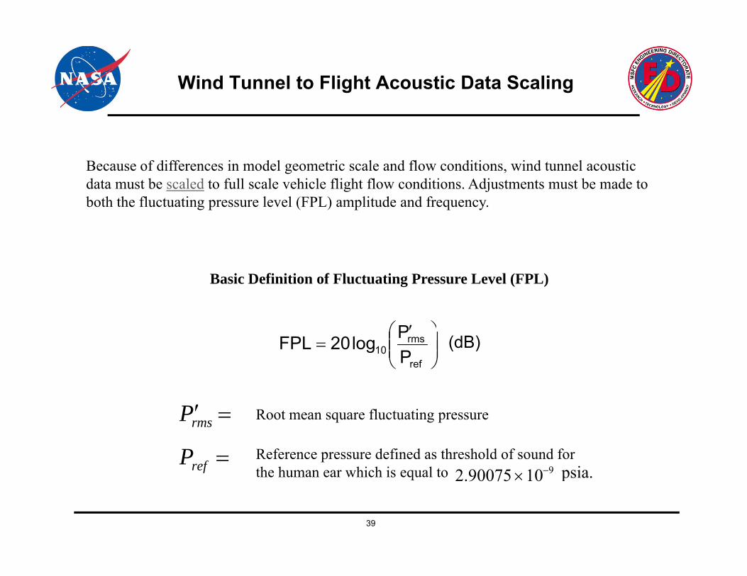
Because of differences in model geometric scale and flow conditions, wind tunnel acoustic d b l d f ll l hi l fli h fl di i Adj b ddata must be scaled to full scale vehicle flight flow conditions. Adjustments must be made to both the fluctuating pressure level (FPL) amplitude and frequency.

Basic Definition of Fluctuating Pressure Level (FPL)

⎞⎛⎟⎟⎠

⎞⎜⎜⎝

⎛ ′=

ref

rms10 P

Plog20FPL (dB)

′ P rms = Root mean square fluctuating pressure

Reference pressure defined as threshold of sound forth h hi h i l t 2 90075 10 9 i

Pref =

39

the human ear which is equal to 2.90075 ×10−9 psia.ref