0 hebbian learning and plasticity - semantic scholar · 0 hebbian learning and plasticity ... from...

0

Hebbian Learning and Plasticity

Wulfram Gerstner

School of Computer and Communication Sciencesand Brain-Mind Institute

Ecole Polytechnique Federale de Lausanne1015 Lausanne EPFL

[email protected]..

To appear in:From Neuron to Cognition via Computational Neuroscience,edited by Michael Arbib and Jimmy Bonaiuto,MIT Press CambridgeChapter 9

Hebbian Learning and Plasticity 1

9. Hebbian Learning and PlasticityThe elementary processing units in the brain are neurons (see Chapter 2)

which are connected to each other via cable-like extensions, called axons anddendrites (see Chapter 3). The contact points between an axon terminal of aneuron A and the dendrite of another neuron B are called synapses. The mostimportant synapses are chemical synapses, but there exist also electrical synapseswhich we will not consider further. When an action potential of neuron A arrivesat the axon terminating at a chemical synapse, a chemical signal (neurotransmit-ter) is ejected into the synaptic cleft and taken up by receptors sitting on themembrane of the dendrite of the receiving neuron. Upon transmitter binding,an ion channel opens, ions flow into the cell and cause a change in the proper-ties of neuron B. This change can be measured as an Excitatory or InhibitoryPostsynaptic Potential (EPSP or IPSP) at the soma of the receiving neuron (seeChapter 3). The strength of an excitatory synaptic connection can be quantifiedby the amplitude of the EPSP. The most important insight for all the rest ofchapter is that the strength of a synapse is not fixed, but can change.

9.1 Introduction to Hebbian Plasticity

Changes of synapses in the network of neurons in the brain are called synapticplasticity. These changes are thought to be the basis of learning.

9.1.1 What is Learning?

A small child learns to unscrew the lid of a bottle. An older child learns to ridea bicycle, to ski, or to skateboard. Learning activities such as in these examplestypically uses an internal reward system of the brain: it hurts if we fall from thebicycle and we are happy if we achieve for the first time a slalom slope with theskies.

Learning is also the basis of factual and episodic memories: we know thename of the current president of the United States because we have heard it oftenenough; we know the date of the French Revolution because we have learned it inschool etc. These are examples of factual memories. We can remember the firstday we went to school; we can recall a beautiful scene encountered during ourlast vacation. These are examples of episodic memories, that have been generatedmost often without explicit learning, but are still acquired (as opposed to inborn)and have therefore been ’learned’ in the loose sense of the word.

Finally, it is the result of learning if a musician is able to distinguish betweentones that sound absolutely identical to the ear of a normal untrained human.In experiments with monkeys measurable differences were found between theauditory areas of animals exposed to specific tones and others living in a normalenvironment (Recanzone et al., 1993). More generally, it is believed that thecortex adapts itself such that more neurons are devoted to stimuli that appearmore frequently or are more important and less neurons to less relevant ones(Buonomano and Merzenich, 1998). This adaptation of cortex (see Chapter 14,Neural Maps) is also subsumed under the term of ’learning’ in the wider sense.

Most likely, all the different forms of learning that we have mentioned (action

2 W. Gerstner (2011) - Hebbian Learning and Plasticity

A Bpre j

post

i

ijw

50ms

Long-term plasticity:

changes persist

30 min

Synapse ijw

time

EPSP

Classification of Plasticity:Short-Term vs. Long-Term

Changes

- induced over 0.1-0.5s

- recover over 1 sec

Protocol

- presynaptic spikes

Changes

- induced over 0.5-5s

- remains over hours

Protocol

- presyn. spikes+‘post’

(Hebbian)

30 min 1 s

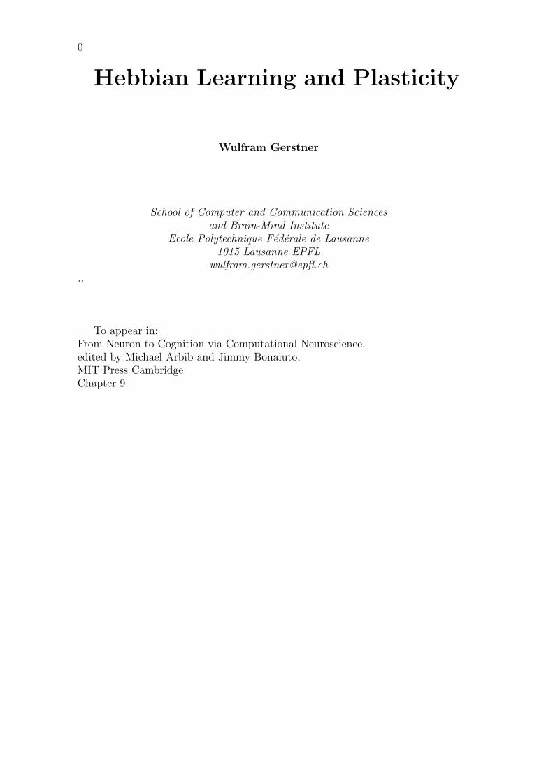
Fig. 9.1: A. Two neurons, a presynaptic neuron j and a postsynaptic neuron i are connectedby a synapse with weight wij . The weight is determined by the amplitude of the excitatorypostsynaptic potential (EPSP) that is measured as the response of the postsynaptic neuron toan isolated input spike (inset lower right). The synapse itself functions via a chemical signalingchain (inset lower left). The weight of the synapse is changed if the two neurons are activatedin the sequence pre- before postsynaptic neuron. B. Short-Term plasticity recovers rapidlywhereas Long-Term plasticity persists for a long time.

learning, formation of factual or episodic memories, adaptation of cortical orga-nization) are in one way or other related to changes in the strength of synapses.

9.1.2 Classification of Synaptic Plasticity

Changes in synaptic strength can be induced in a controlled way in preparationsof neuronal brain slices. First, the strength of the connection is measured by gen-erating a single test spike in the presynaptic (=signaling) neuron while recordingthe postsynaptic potential (or postsynaptic current) in the postsynaptic (=re-ceiving) neuron. Then an appropriate stimulus is given to induce a change of thesynapse. Finally, a second test spike is evoked in the presynaptic neuron and thechange in the amplitude of the postsynaptic potential is noted; see Fig. 9.1.

An appropriate stimulus, for example, a sequence of 10 spikes at 100 Hz inthe presynaptic neuron, can increase or decrease the amplitude of the measuredEPSP by a factor of two or more. However, if another test pulse is given 5seconds later, this change has disappeared (Markram et al., 1998; Abbott et al.,1997). Since this type of plasticity lasts only for one or a few seconds, it is calledshort-term plasticity (Fig. 9.1B).

We now consider a different stimulus. The presynaptic neuron is stimulatedso as to produce 60 spikes at 20Hz. In parallel the postsynaptic neuron is alsostimulated to produce 60 spikes at 20Hz, but the two stimulation protocols areslightly shifted so that the postsynaptic neuron fires always 10ms after the presy-naptic one (Fig. 9.1A). Note that the stimulus only lasts three seconds in total.Nevertheless, it introduces an increase in the EPSP that persists for minutesor hours. Hence it is an example of persistent plasticity, also called Long-TermPotentiation (LTP). If the relative timing is reversed so that the presynaptic neu-ron fires always after the postsynaptic one, the protocol with 60 spikes inducesLong-Term Depression (LTD).

The specific protocol discussed here is called Spike Timing Dependent Plas-ticity (STDP) (Markram et al., 1997; Abbott and Nelson, 2000), but it is onlyone example of a much broader class of stimulation protocols that are all suitableto induce LTP and LTD. Instead of driving the postsynaptic neuron to firing, it


can also be held at weakly or strongly depolarized level. If the depolarization iscombined with presynaptic spike arrival, this causes LTD or LTP (Artola et al.,1990; Ngezahayo et al., 2000). Instead of controlling both presynaptic and post-synaptic neurons precisely, one can also stimulate many presynaptic fibers by ahigh-frequency sequence of extracellular current pulses while recording (intracel-lularly or extracullarly) from postsynaptic neurons. If enough presynaptic fibersare stimulated, the postsynaptic neuron is depolarized or even firing, and LTPcan be induced. Such an extracellular stimulation protocol is particularly usefulto confirm that changes induced by LTP or LTD indeed last for many hours (Freyand Morris, 1998).

The first and most important classification is that between short-term plas-ticity and long-term plasticity; see Fig. 9.1B. In the following we will focuson persistent plasticity (LTP and LTD) and neglect short-term plasticity. Butwithin the realm of long-term plasticity further classifications are possible. Wementioned already a distinction between spike-timing based protocols on one sideand traditional protocols on the other side.

Another important distinction is the presence or absence of neuromodulatorsduring the plasticity inducing protocol. We will come back to this distinction inSection 4 of this chapter.

9.1.3 Long-Term Potentiation as Hebbian Learning

LTP and LTD are thought to be the synaptic basis of learning in the brain. Manyexperiments on LTP and LTD, and nearly all synaptic theories of learning, havebeen inspired by a formulation of Hebb (Hebb, 1949) which has roots that canin fact be traced back much further in the past (Makram et al., 2011). It statesthat it would be useful to have a rule that synapses are modified whenever thetwo neurons that are connected to each other are active together. It is sometimessummarized in the slogan ’fire together - wire together’, but the exact wording isworth a read:

When an axon of cell A is near enough to excite cell B or repeatedly or per-sistently takes part in firing it, some growth process or metabolic change takesplace in one or both cells such that A’s efficiency, as one of the cells firing B, isincreased.

In contrast to the compressed slogan it contains a ’causal’ tone, because ’tak-ing part in firing’ the postsynaptic neuron implies that the presynaptic neuronis, at least partly, causing the spike of the postsynaptic one. We will come backto this aspect when we speak more about STDP.

At the moment, two aspects are important. First, for the connection from Ato B only two neurons are important, namely A and B, but not any other neuronC that might make a connection onto A or B. We summarize this insight bysaying that the learning rule is ’local’: only information that is available at thelocation of the synapse can be used to change the weight of that synapse. Second,the wording ’cell A ... takes part in firing’ cell B implies that both cells have tobe active. We summarize this insight by saying that the learning rule must besensitive to the correlations between the action potentials of the two neurons.

With these two aspects in mind, let us now return to the plasticity protocolsfor LTP that we discussed in the previous subsection. Indeed, the STDP protocol


1

2

4

5

6

7

8

10

9

3

5

6

9

4

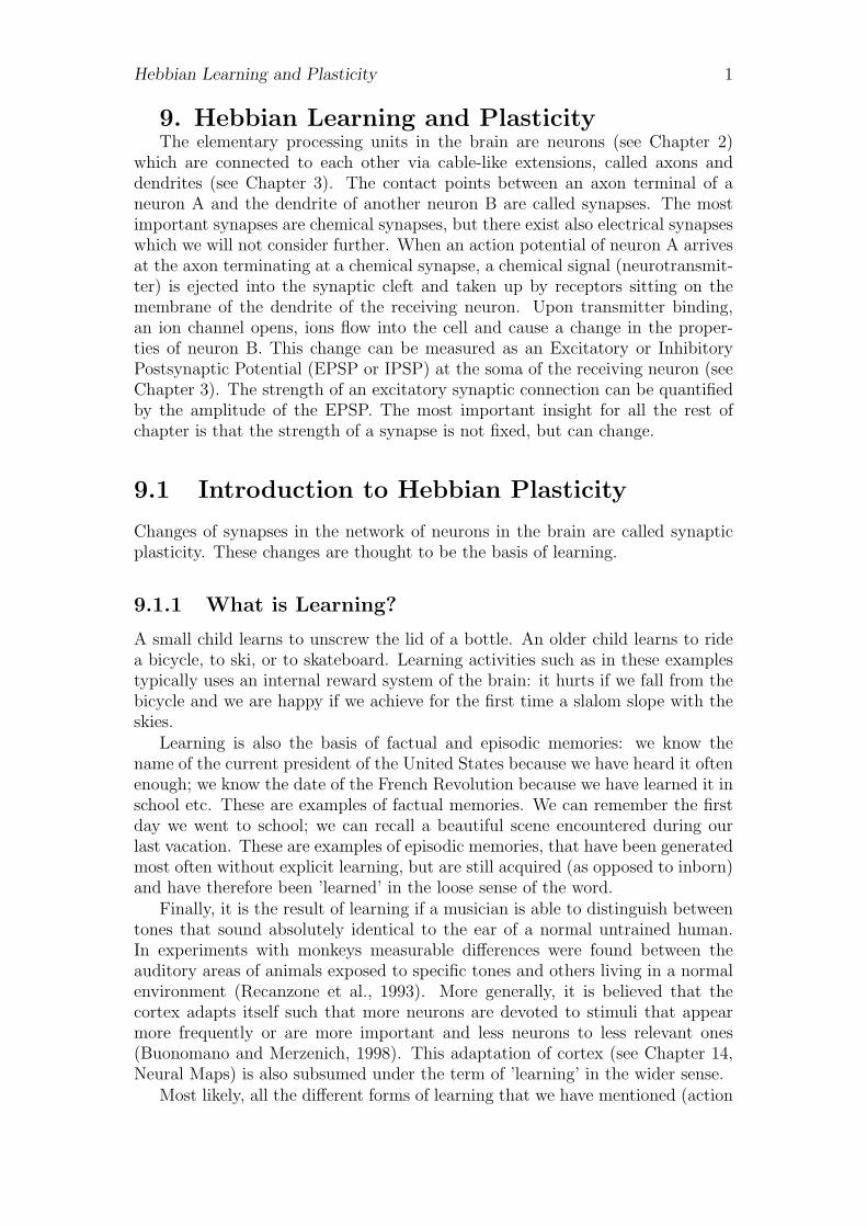
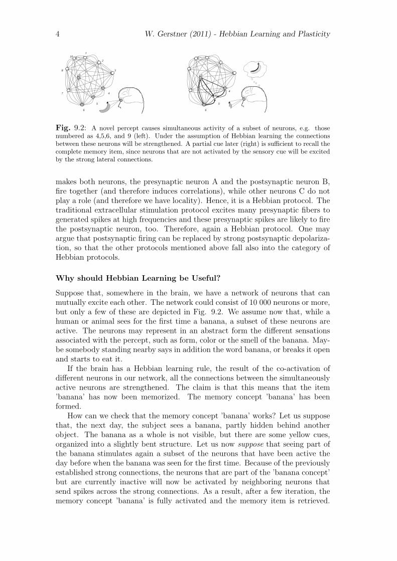
Fig. 9.2: A novel percept causes simultaneous activity of a subset of neurons, e.g. thosenumbered as 4,5,6, and 9 (left). Under the assumption of Hebbian learning the connectionsbetween these neurons will be strengthened. A partial cue later (right) is sufficient to recall thecomplete memory item, since neurons that are not activated by the sensory cue will be excitedby the strong lateral connections.

makes both neurons, the presynaptic neuron A and the postsynaptic neuron B,fire together (and therefore induces correlations), while other neurons C do notplay a role (and therefore we have locality). Hence, it is a Hebbian protocol. Thetraditional extracellular stimulation protocol excites many presynaptic fibers togenerated spikes at high frequencies and these presynaptic spikes are likely to firethe postsynaptic neuron, too. Therefore, again a Hebbian protocol. One mayargue that postsynaptic firing can be replaced by strong postsynaptic depolariza-tion, so that the other protocols mentioned above fall also into the category ofHebbian protocols.

Why should Hebbian Learning be Useful?

Suppose that, somewhere in the brain, we have a network of neurons that canmutually excite each other. The network could consist of 10 000 neurons or more,but only a few of these are depicted in Fig. 9.2. We assume now that, while ahuman or animal sees for the first time a banana, a subset of these neurons areactive. The neurons may represent in an abstract form the different sensationsassociated with the percept, such as form, color or the smell of the banana. May-be somebody standing nearby says in addition the word banana, or breaks it openand starts to eat it.

If the brain has a Hebbian learning rule, the result of the co-activation ofdifferent neurons in our network, all the connections between the simultaneouslyactive neurons are strengthened. The claim is that this means that the item’banana’ has now been memorized. The memory concept ’banana’ has beenformed.

How can we check that the memory concept ’banana’ works? Let us supposethat, the next day, the subject sees a banana, partly hidden behind anotherobject. The banana as a whole is not visible, but there are some yellow cues,organized into a slightly bent structure. Let us now suppose that seeing part ofthe banana stimulates again a subset of the neurons that have been active theday before when the banana was seen for the first time. Because of the previouslyestablished strong connections, the neurons that are part of the ’banana concept’but are currently inactive will now be activated by neighboring neurons thatsend spikes across the strong connections. As a result, after a few iteration, thememory concept ’banana’ is fully activated and the memory item is retrieved.


The basic idea of memory retrieval discussed here is at the heart of models ofworking memory and long-term memory (see Chapter 13).

A Family of Hebbian Rules

Hebb was a theoretically inclined psychologist, who developed the essential in-sights of why the principle, which we now call the Hebb-rule, would be useful; buthe was not a mathematician and never wrote down a mathematical formulationof his rule. Finding an appropriate mathematical description is our task now. Inthis subsection we follow closely the treatment in Chapter 10.2 of Gerstner andKistler (2002).

In order to find a mathematically formulated learning rule based on Hebb’spostulate we focus on a single synapse with efficacy wij that transmits signalsfrom a presynaptic neuron j to a postsynaptic neuron i. For the moment wefocus on a description in terms of mean firing rates. In the following, the activityof the presynaptic neuron is denoted by νj and that of the postsynaptic neuronby νi.

As mentioned before, there are two aspects in Hebb’s postulate that are partic-ularly important, viz. locality and cooperativity. Locality means that the changeof the synaptic efficacy can only depend on local variables, i.e., on informationthat is available at the site of the synapse, such as pre- and postsynaptic firingrate, and the actual value of the synaptic efficacy, but not on the activity of otherneurons. Based on the locality of Hebbian plasticity we can make a rather generalansatz for the change of the synaptic efficacy,

d

dtwij = F (wij; νi, νj) . (9.1)

Here, dwij/dt is the rate of change of the synaptic coupling strength and F is aso far undetermined function.

We may wonder whether there are other local variables (e.g., the membranepotential ui) that should be included as additional arguments of the functionF . It turns out that in standard rate models this is not necessary, since themembrane potential ui is uniquely determined by the postsynaptic firing rate,νi = g(ui), with a monotone gain function g.

The second important aspect of Hebb’s postulate, cooperativity, implies thatpre- and postsynaptic neuron have to be active simultaneously for a synapticweight change to occur. We can use this property to learn something about thefunction F . If F is sufficiently well-behaved, we can expand F in a Taylor seriesabout νi = νj = 0,

d

dtwij = c0(wij) + cpost

1 (wij)νi + cpre1 (wij) νj

+cpre2 (wij) ν

2j + cpost

2 (wij) ν2i + ccorr

2 (wij) νi νj +O(ν3) . (9.2)

The term containing ccorr2 on the right-hand side of (9.2) is bilinear in pre- and

postsynaptic activity. This term implements the AND condition for cooperativitywhich makes Hebbian learning a useful concept.


The simplest choice for our function F is to fix ccorr2 at a positive constant and

to set all other terms in the Taylor expansion to zero. The result is the prototypeof Hebbian learning,

d

dtwij = ccorr

2 νi νj . (9.3)

The dependence of F on the synaptic efficacy wij is a natural consequenceof the fact that wij has to be bounded. If F were independent of wij, thenthe synaptic efficacy would grow without limit if the same potentiating stimulusis applied over and over again. Explosion of weights can be avoided by ’hardbounds’: ccorr

2 (wij) = γ2 > 0 for 0 < wij < 1 and zero otherwise. A more subtlesaturation of synaptic weights can be achieved, if the parameter ccorr

2 in Eq. (9.2)tends to zero as wij approaches its maximum value, say wmax = 1, e.g.,

ccorr2 (wij) = γ2 (1− wij) (9.4)

with a positive constant γ2. An interpolation between the soft bounds and hardbounds can be implemented by writing ccorr

2 (wij) = γ2 (1−wij)η with a parameter0 ≤ η ≤ 1. For η = 0 we retrieve the hard bounds while for η = 1 we are back tothe linear soft bounds.

Obviously, setting all parameters except ccorr2 to zero is a very special case of

the general framework developed in Eq. (9.2). Are there other ’Hebbian’ learningrules in this framework?

First we note that a learning rule with ccorr2 = 0 and only first-order terms

(such as cpost1 6= 0 or cpre

1 6= 0) would be called non-Hebbian plasticity, becausepre- or postsynaptic activity alone induces a change of the synaptic efficacy.Hence these learning rules miss the correlation aspect of Hebb’s principle. Thusa learning rule in the family of Eq. (9.2) needs a term ccorr

2 > 0 so as to qualify asHebbian. But more complicated learning rules can be constructed if in additionto the linear terms, and the terms nu2

i or nu2j other terms in the expansion of

Eq. (9.2), such as νi ν2j , ν2

i νj, ν2i ν

2j , etc., are included as well. A learning rule

with a positive coefficient in front of ν2i νj would also qualify as Hebbian, even if

ccorr2 vanishes or is negative, because at high postsynaptic firing rates the positive

correlations dominate the dynamics, as we will see further below in the contextof the Bienenstock-Cooper-Munro rule.

Hebb’s original proposal does not contain a rule for a decrease of synapticweights. In a system where synapses can only be strengthened, all efficacieswill finally saturate at their upper maximum value. An option of decreasing theweights (synaptic depression) is therefore a necessary requirement for any usefullearning rule. This can, for example, be achieved by weight decay, which can beimplemented in Eq. (9.2) by setting

c0(wij) = −γ0wij . (9.5)

Here, γ0 is (small) positive constant that describes the rate by which wij decaysback to zero in the absence of stimulation. Our formulation (9.2) is hence suffi-ciently general to allow for a combination of synaptic potentiation and depression.If we combine (9.4) and (9.5) we obtain the learning rule

d

dtwij = ccorr

2 (wij) νi νj − γ0wij . (9.6)


The last term leads to an exponential decay to wij = 0 in the absence of stimu-lation, only one of the two neurons is active.

Another interesting aspect of learning rules is competition. The idea is thatsynaptic weights can only grow at the expense of others so that if a certain sub-group of synapses is strengthened, other synapses to the same postsynaptic neuronhave to be weakened. Competition is essential for any form of self-organizationand pattern formation. Practically, competition can be implemented in simula-tions by normalizing by an explicit algebraic step the sum of all weights convergingonto the same postsynaptic neuron (Miller and MacKay, 1994). Though this canbe motivated by a limitation of common synaptic resources such a learning ruleviolates locality of synaptic plasticity. Much more elegant, however, is a formula-tion that remains local, but makes use of the second-order term ν2

i in Eq. (9.2).Specifically, we take ccorr

2 = γ > 0 and cpost2 = −γ wij and set all other parameters

to zero. The learning rule

d

dtwij = γ [νi νj − wij ν2

i ] (9.7)

is called Oja’s rule (Oja, 1982). If combined with a linear model neuron, Oja’s ruleconverges asymptotically to synaptic weights that are normalized to

∑j w

2ij = 1

while keeping the essential Hebbian properties of the standard rule of Eq. (9.3).We note that normalization of

∑j w

2ij implies competition between the synapses

that make connections to the same postsynaptic neuron, i.e., if some weights growothers must decrease.

9.1.4 The Bienenstock-Cooper-Munro Rule as an Exam-ple of Hebbian Learning

Higher terms in the expansion on the right-hand side of Eq. (9.2) lead to moreintricate plasticity schemes. As an example, let us consider the Bienenstock-Cooper-Munro rule

d

dtwij = η φ(νi) νj − γ wij (9.8)

with a nonlinear function φ(νi) which we take as φ(νi) = νi (νi − θ) and a pa-rameter θ as a reference rate (Bienenstock et al., 1982). A simple calculationshows that Eq. (9.8) can be classified in the framework of Eq. (9.2) with a termccorr2 = −ηνθ and a higher-order term proportional to ν2

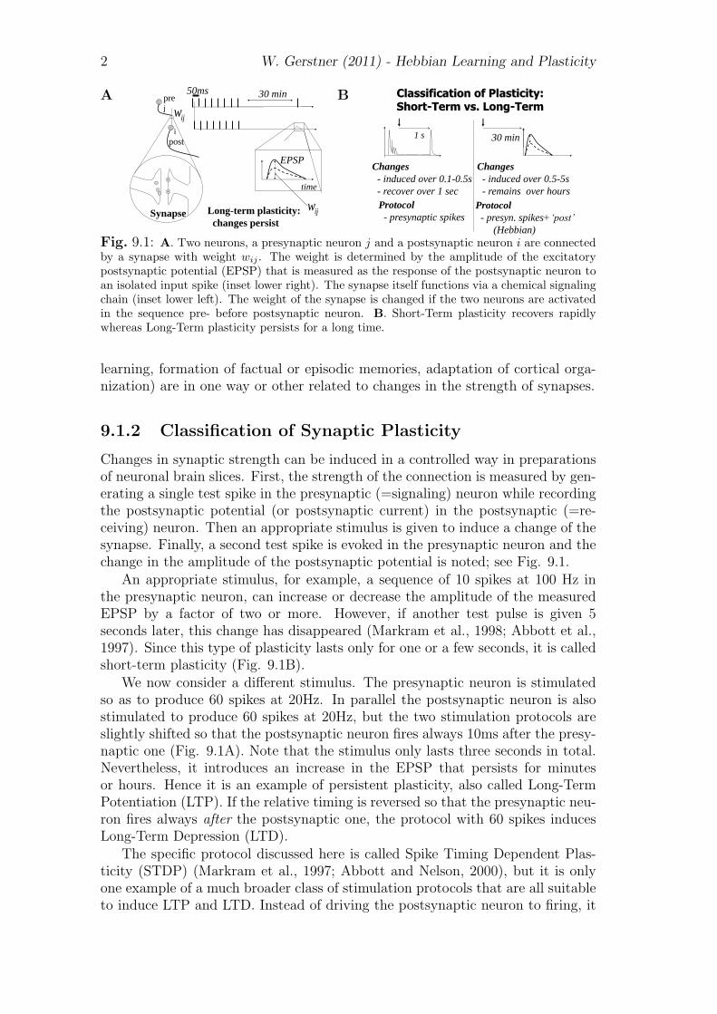
i νj that comes with apositive coefficient η > 0. What does this learning rule do? If the presynapticneuron is inactive (νj = 0), the synaptic weight does not change. Let us nowsuppose that the presynaptic neuron is active (νj > 0) while at the same time thepostsynaptic neuron is firing at a high rate νi > θ (see Fig. 9.3). The synapticweight increases since both neurons are jointly active. Hence it is a Hebbian rule.If the presynaptic neuron is firing while the postsynaptic neuron is only weaklyactive (νi < θ), then the synaptic weight decreases. Thus the parameter θ marksthe transition point between the induction of LTD and LTP.

In order to get an understanding of how Hebbian plasticity works, the readeris asked to turn now to the first exercise.

Two important insights can be derived from an analysis of Eq. (9.8) [see alsoExercise 1 for an intuitive approach].


A B{

{

i

ijdw

dt

i

j ijw

{

{ i

{

{ i

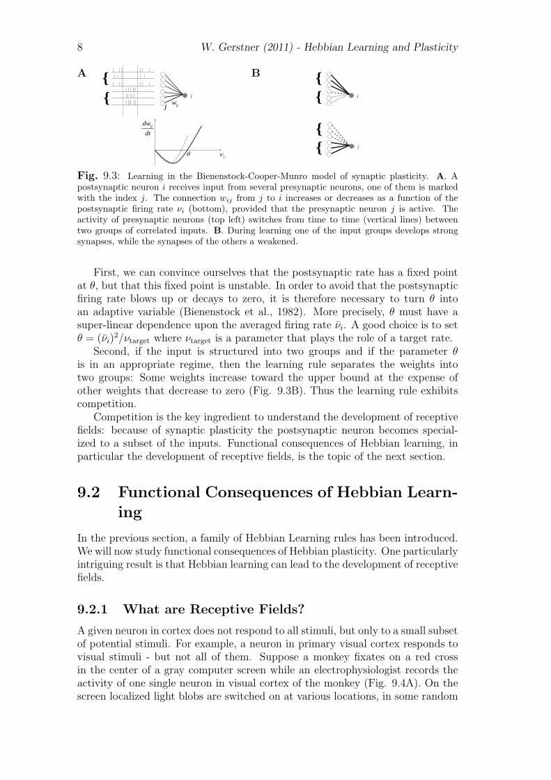
Fig. 9.3: Learning in the Bienenstock-Cooper-Munro model of synaptic plasticity. A. Apostsynaptic neuron i receives input from several presynaptic neurons, one of them is markedwith the index j. The connection wij from j to i increases or decreases as a function of thepostsynaptic firing rate νi (bottom), provided that the presynaptic neuron j is active. Theactivity of presynaptic neurons (top left) switches from time to time (vertical lines) betweentwo groups of correlated inputs. B. During learning one of the input groups develops strongsynapses, while the synapses of the others a weakened.

First, we can convince ourselves that the postsynaptic rate has a fixed pointat θ, but that this fixed point is unstable. In order to avoid that the postsynapticfiring rate blows up or decays to zero, it is therefore necessary to turn θ intoan adaptive variable (Bienenstock et al., 1982). More precisely, θ must have asuper-linear dependence upon the averaged firing rate νi. A good choice is to setθ = (νi)

2/νtarget where νtarget is a parameter that plays the role of a target rate.Second, if the input is structured into two groups and if the parameter θ

is in an appropriate regime, then the learning rule separates the weights intotwo groups: Some weights increase toward the upper bound at the expense ofother weights that decrease to zero (Fig. 9.3B). Thus the learning rule exhibitscompetition.

Competition is the key ingredient to understand the development of receptivefields: because of synaptic plasticity the postsynaptic neuron becomes special-ized to a subset of the inputs. Functional consequences of Hebbian learning, inparticular the development of receptive fields, is the topic of the next section.

9.2 Functional Consequences of Hebbian Learn-ing

In the previous section, a family of Hebbian Learning rules has been introduced.We will now study functional consequences of Hebbian plasticity. One particularlyintriguing result is that Hebbian learning can lead to the development of receptivefields.

9.2.1 What are Receptive Fields?

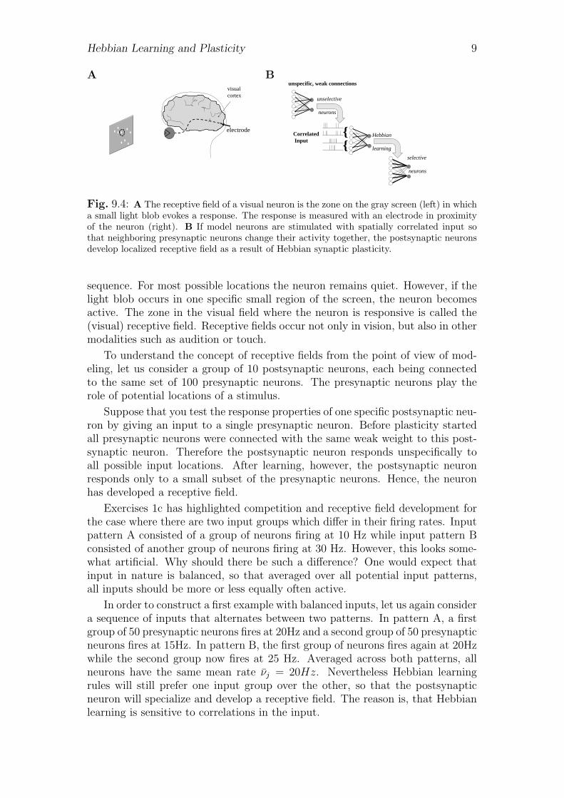
A given neuron in cortex does not respond to all stimuli, but only to a small subsetof potential stimuli. For example, a neuron in primary visual cortex responds tovisual stimuli - but not all of them. Suppose a monkey fixates on a red crossin the center of a gray computer screen while an electrophysiologist records theactivity of one single neuron in visual cortex of the monkey (Fig. 9.4A). On thescreen localized light blobs are switched on at various locations, in some random


A Bvisual

cortex

electrode

unselective

neurons

unspecific, weak connections

Correlated

Input

{{

Hebbian

learning

selective

neurons

Fig. 9.4: A The receptive field of a visual neuron is the zone on the gray screen (left) in whicha small light blob evokes a response. The response is measured with an electrode in proximityof the neuron (right). B If model neurons are stimulated with spatially correlated input sothat neighboring presynaptic neurons change their activity together, the postsynaptic neuronsdevelop localized receptive field as a result of Hebbian synaptic plasticity.

sequence. For most possible locations the neuron remains quiet. However, if thelight blob occurs in one specific small region of the screen, the neuron becomesactive. The zone in the visual field where the neuron is responsive is called the(visual) receptive field. Receptive fields occur not only in vision, but also in othermodalities such as audition or touch.

To understand the concept of receptive fields from the point of view of mod-eling, let us consider a group of 10 postsynaptic neurons, each being connectedto the same set of 100 presynaptic neurons. The presynaptic neurons play therole of potential locations of a stimulus.

Suppose that you test the response properties of one specific postsynaptic neu-ron by giving an input to a single presynaptic neuron. Before plasticity startedall presynaptic neurons were connected with the same weak weight to this post-synaptic neuron. Therefore the postsynaptic neuron responds unspecifically toall possible input locations. After learning, however, the postsynaptic neuronresponds only to a small subset of the presynaptic neurons. Hence, the neuronhas developed a receptive field.

Exercises 1c has highlighted competition and receptive field development forthe case where there are two input groups which differ in their firing rates. Inputpattern A consisted of a group of neurons firing at 10 Hz while input pattern Bconsisted of another group of neurons firing at 30 Hz. However, this looks some-what artificial. Why should there be such a difference? One would expect thatinput in nature is balanced, so that averaged over all potential input patterns,all inputs should be more or less equally often active.

In order to construct a first example with balanced inputs, let us again considera sequence of inputs that alternates between two patterns. In pattern A, a firstgroup of 50 presynaptic neurons fires at 20Hz and a second group of 50 presynapticneurons fires at 15Hz. In pattern B, the first group of neurons fires again at 20Hzwhile the second group now fires at 25 Hz. Averaged across both patterns, allneurons have the same mean rate νj = 20Hz. Nevertheless Hebbian learningrules will still prefer one input group over the other, so that the postsynapticneuron will specialize and develop a receptive field. The reason is, that Hebbianlearning is sensitive to correlations in the input.


9.2.2 Correlations and Principal Component Analysis

We now turn to a formal derivation of the functional properties of Hebbian learn-ing rules. We show mathematically that simple models of Hebbian learning aresensitive to correlations in the input. More precisely, a standard Hebb rule com-bined with a linear rate model for the postsynaptic neuron performs PrincipalComponent Analysis, also called PCA. This section follows closely the text inChapter 11.1 of Gerstner and Kistler (2002).

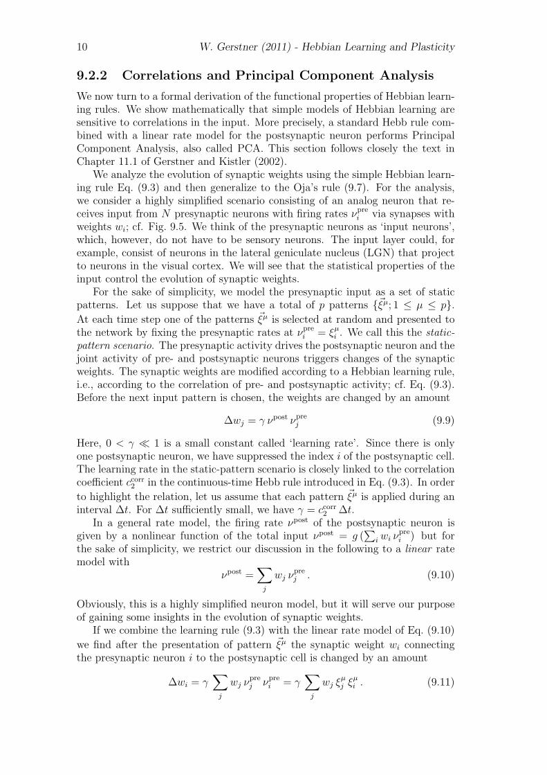
We analyze the evolution of synaptic weights using the simple Hebbian learn-ing rule Eq. (9.3) and then generalize to the Oja’s rule (9.7). For the analysis,we consider a highly simplified scenario consisting of an analog neuron that re-ceives input from N presynaptic neurons with firing rates νpre

i via synapses withweights wi; cf. Fig. 9.5. We think of the presynaptic neurons as ‘input neurons’,which, however, do not have to be sensory neurons. The input layer could, forexample, consist of neurons in the lateral geniculate nucleus (LGN) that projectto neurons in the visual cortex. We will see that the statistical properties of theinput control the evolution of synaptic weights.

For the sake of simplicity, we model the presynaptic input as a set of staticpatterns. Let us suppose that we have a total of p patterns {~ξµ; 1 ≤ µ ≤ p}.At each time step one of the patterns ~ξµ is selected at random and presented tothe network by fixing the presynaptic rates at νpre

i = ξµi . We call this the static-pattern scenario. The presynaptic activity drives the postsynaptic neuron and thejoint activity of pre- and postsynaptic neurons triggers changes of the synapticweights. The synaptic weights are modified according to a Hebbian learning rule,i.e., according to the correlation of pre- and postsynaptic activity; cf. Eq. (9.3).Before the next input pattern is chosen, the weights are changed by an amount

∆wj = γ νpost νprej (9.9)

Here, 0 < γ � 1 is a small constant called ‘learning rate’. Since there is onlyone postsynaptic neuron, we have suppressed the index i of the postsynaptic cell.The learning rate in the static-pattern scenario is closely linked to the correlationcoefficient ccorr

2 in the continuous-time Hebb rule introduced in Eq. (9.3). In order

to highlight the relation, let us assume that each pattern ~ξµ is applied during aninterval ∆t. For ∆t sufficiently small, we have γ = ccorr

2 ∆t.In a general rate model, the firing rate νpost of the postsynaptic neuron is

given by a nonlinear function of the total input νpost = g (∑

iwi νprei ) but for

the sake of simplicity, we restrict our discussion in the following to a linear ratemodel with

νpost =∑j

wj νprej . (9.10)

Obviously, this is a highly simplified neuron model, but it will serve our purposeof gaining some insights in the evolution of synaptic weights.

If we combine the learning rule (9.3) with the linear rate model of Eq. (9.10)

we find after the presentation of pattern ~ξµ the synaptic weight wi connectingthe presynaptic neuron i to the postsynaptic cell is changed by an amount

∆wi = γ∑j

wj νprej νpre

i = γ∑j

wj ξµj ξ

µi . (9.11)


A B

1

2

3

...

j

N

post

i

post

i

total input

p input

patterns

1

2

3

...

j

N

{ ;1 }p

prekk ik

posti w

linear neuron

model

Fig. 9.5: A. Patterns ~ξµ are applied as a set of presynaptic firing rates νj , i.e., ~ξµj = νµj for1 ≤ j ≤ N . The output rate of the postsynaptic neuron is taken as a linear function of thetotal input, an approximation to a sigmoidal gain function. Adapted from Gerstner and Kistler(2002). B Patterns are applied one after the other in a sequence.

The evolution of the weight vector ~w = (w1, . . . , wN) is thus determined by theiteration

wi(n+ 1) = wi(n) + γ∑j

wj ξµn

j ξµn

i , (9.12)

where µn denotes the pattern that is presented during the nth time step.We are interested in the long-term behavior of the synaptic weights. To this

end we assume that the weight vector evolves along a more or less deterministictrajectory with only small stochastic deviations that result from the randomnessat which new input patterns are chosen. This is, for example, the case if thelearning rate is small so that a large number of patterns has to be presented inorder to induce a substantial weight change. In such a situation it is sensible toconsider the expectation value of the weight vector, i.e., the weight vector 〈~w(n)〉averaged over the sequence (~ξµ1 , ~ξµ2 , . . . , ~ξµn) of all patterns that so far have beenpresented to the network. From (9.12) we find

〈wi(n+ 1)〉 = 〈wi(n)〉+ γ∑

j

⟨wj(n) ξ

µn+1

j ξµn+1

i

⟩= 〈wi(n)〉+ γ

∑j 〈wj(n)〉

⟨ξµn+1

j ξµn+1

i

⟩= 〈wi(n)〉+ γ

∑j Cij 〈wj(n)〉 . (9.13)

The angular brackets denote an ensemble average over the whole sequence of inputpatterns (~ξµ1 , ~ξµ2 , . . . ). The second equality is due to the fact that input patternsare chosen independently in each time step, so that the average over wj(n) and(ξµn+1

j ξµn+1

i ) can be factorized. In the final expression we have introduced thecorrelation matrix Cij,

Cij =1

p

p∑µ=1

ξµi ξµj =

⟨ξµi ξ

µj

⟩µ. (9.14)

Expression (9.13) can be written in a more compact form using matrix notation,

〈~w(n+ 1)〉 = (1I + γ C) 〈~w(n)〉 = (1I + γ C)n+1 〈~w(0)〉 , (9.15)

where ~w(n) = (w1(n), . . . , wN(n)) is the weight vector and 1I is the identitymatrix.


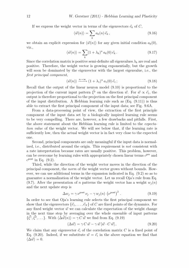
If we express the weight vector in terms of the eigenvectors ~ek of C,

〈~w(n)〉 =∑k

ak(n)~ek , (9.16)

we obtain an explicit expression for 〈~w(n)〉 for any given initial condition ak(0),viz.,

〈~w(n)〉 =∑k

(1 + λk)n ak(0)~ek . (9.17)

Since the correlation matrix is positive semi-definite all eigenvalues λk are real andpositive. Therefore, the weight vector is growing exponentially, but the growthwill soon be dominated by the eigenvector with the largest eigenvalue, i.e., thefirst principal component,

〈~w(n)〉 n→∞−−−→ (1 + λ1)n a1(0)~e1 ; (9.18)

Recall that the output of the linear neuron model (9.10) is proportional to the

projection of the current input pattern ~ξµ on the direction ~w. For ~w ∝ ~e1, theoutput is therefore proportional to the projection on the first principal componentof the input distribution. A Hebbian learning rule such as (Eq. (9.11)) is thusable to extract the first principal component of the input data; see Fig. 9.6A.

From a data-processing point of view, the extraction of the first principlecomponent of the input data set by a biologically inspired learning rule seemsto be very compelling. There are, however, a few drawbacks and pitfalls. First,the above statement about the Hebbian learning rule is limited to the expecta-tion value of the weight vector. We will see below that, if the learning rate issufficiently low, then the actual weight vector is in fact very close to the expectedone.

Second, principal components are only meaningful if the input data is normal-ized, i.e., distributed around the origin. This requirement is not consistent witha rate interpretation because rates are usually positive. This problem, however,can be overcome by learning rules with appropriately chosen linear terms cpre andcpost in Eq. (9.2).

Third, while the direction of the weight vector moves in the direction of theprincipal component, the norm of the weight vector grows without bounds. How-ever, we can use additional terms in the expansion indicated in Eq. (9.2) so as toguarantee a normalization of the weight vector. Let us recall Oja’s rule from Eq.(9.7). After the presentation of n patterns the weight vector has a weight wj(n)and the next update step is

∆wj = γ νpost νj − γ wj(n)(νpost

)2. (9.19)

In order to see that Oja’s learning rule selects the first principal component weshow that the eigenvectors {~e1, . . . , ~eN} of C are fixed points of the dynamics. Forany fixed weight vector ~w we can calculate the expectation of the weight changein the next time step by averaging over the whole ensemble of input patterns{~ξ1, ~ξ2, . . . }. With 〈∆ ~w(n)〉 = γ C ~w we find from Eq. (9.19)

〈∆~w〉 = γ C ~w − γ ~w [~w · C ~w] , (9.20)

We claim that any eigenvector ~ei of the correlation matrix C is a fixed point ofEq. (9.20). Indeed, if we substitute ~w = ~ei in the above equation we find that〈∆~w〉 = 0.


A B

1

1

p

kj k j k jpC

2x

1x

3x

nnn eeC

0

N ...21

= Principal Component1e

0 ( )( )kj k k j jC

{ ;1 }p

3

1e

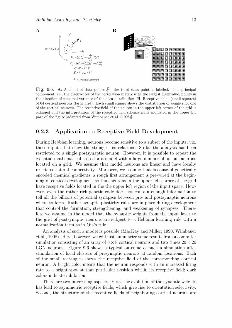
Fig. 9.6: A. A cloud of data points ~ξµ, the third data point is labeled. The principalcomponent, i.e., the eigenvector of the correlation matrix with the largest eigenvalue, points inthe direction of maximal variance of the data distribution. B. Receptive fields (small squares)of 64 cortical neurons (large grid). Each small square shows the distribution of weights for oneof the cortical neurons. The receptive field of the neuron in the upper left corner of the grid isenlarged and the interpretation of the receptive field schematically indicated in the upper leftpart of the figure [adapted from Wimbauer et al. (1998)].

9.2.3 Application to Receptive Field Development

During Hebbian learning, neurons become sensitive to a subset of the inputs, viz.those inputs that show the strongest correlations. So far the analysis has beenrestricted to a single postsynaptic neuron. However, it is possible to repeat theessential mathematical steps for a model with a large number of output neuronslocated on a grid. We assume that model neurons are linear and have locallyrestricted lateral connectivity. Moreover, we assume that because of geneticallyencoded chemical gradients, a rough first arrangement is pre-wired at the begin-ning of cortical development, so that neurons in the upper left corner of the gridhave receptive fields located in the the upper left region of the input space. How-ever, even the rather rich genetic code does not contain enough information totell all the billions of potential synapses between pre- and postsynaptic neuronswhere to form. Rather synaptic plasticity rules are in place during developmentthat control the formation, strengthening, and weakening of synapses. There-fore we assume in the model that the synaptic weights from the input layer tothe grid of postsynaptic neurons are subject to a Hebbian learning rule with anormalization term as in Oja’s rule.

An analysis of such a model is possible (MacKay and Miller, 1990; Wimbaueret al., 1998). Here, however, we will just summarize some results from a computersimulation consisting of an array of 8× 8 cortical neurons and two times 20× 20LGN neurons. Figure 9.6 shows a typical outcome of such a simulation afterstimulation of local clusters of presynaptic neurons at random locations. Eachof the small rectangles shows the receptive field of the corresponding corticalneuron. A bright color means that the neuron responds with an increased firingrate to a bright spot at that particular position within its receptive field; darkcolors indicate inhibition.

There are two interesting aspects. First, the evolution of the synaptic weightshas lead to asymmetric receptive fields, which give rise to orientation selectivity.Second, the structure of the receptive fields of neighboring cortical neurons are


A B

pre

j

posti

ijw

Pre

before post

post

i

pre

j tt

pre

jt

post

i

pre

j tt

post

i

pre

j tt

0

)(posti

prejij ttWw

0

pre

j

iijw

f

jt

f

it

Pre

before post

post

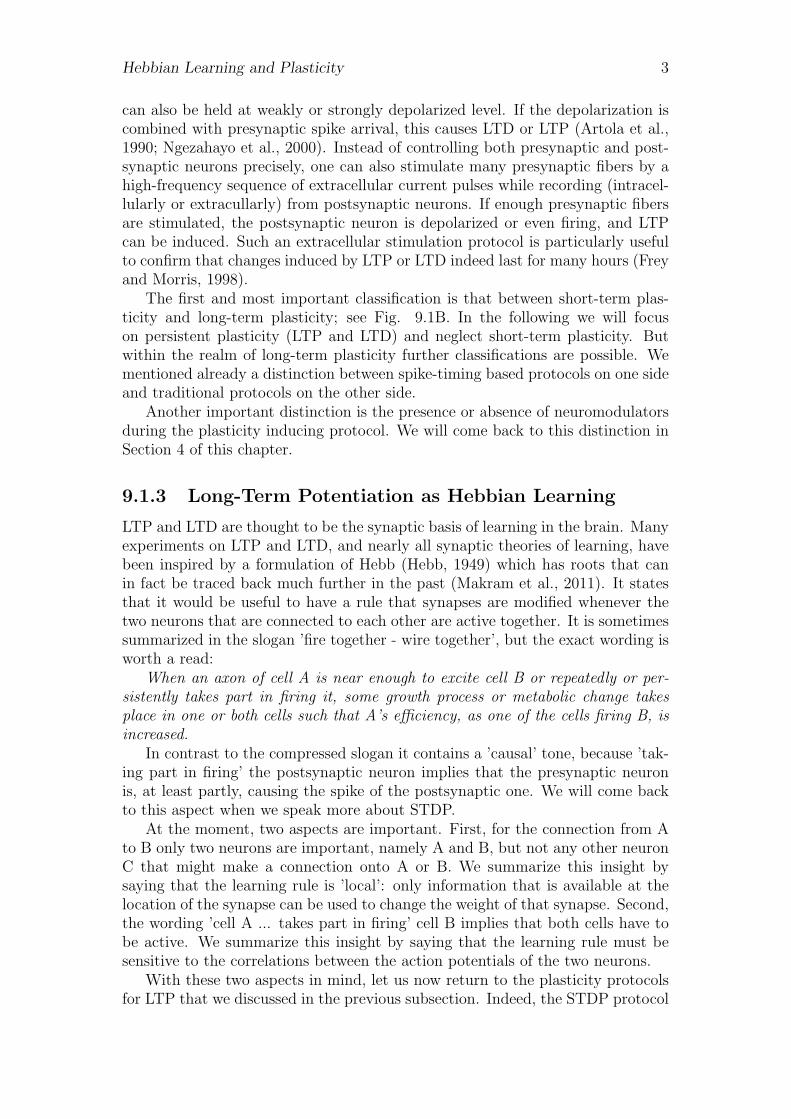
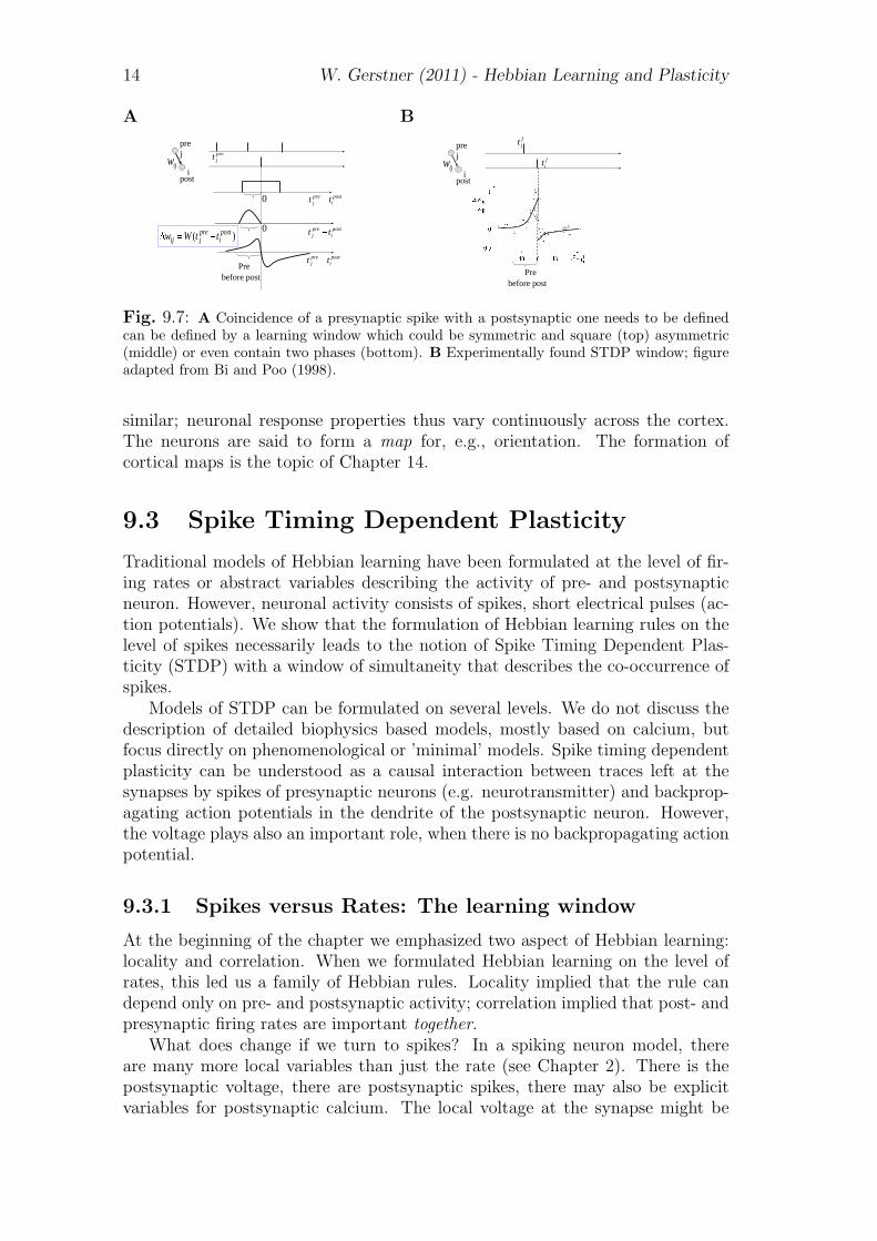
Fig. 9.7: A Coincidence of a presynaptic spike with a postsynaptic one needs to be definedcan be defined by a learning window which could be symmetric and square (top) asymmetric(middle) or even contain two phases (bottom). B Experimentally found STDP window; figureadapted from Bi and Poo (1998).

similar; neuronal response properties thus vary continuously across the cortex.The neurons are said to form a map for, e.g., orientation. The formation ofcortical maps is the topic of Chapter 14.

9.3 Spike Timing Dependent Plasticity

Traditional models of Hebbian learning have been formulated at the level of fir-ing rates or abstract variables describing the activity of pre- and postsynapticneuron. However, neuronal activity consists of spikes, short electrical pulses (ac-tion potentials). We show that the formulation of Hebbian learning rules on thelevel of spikes necessarily leads to the notion of Spike Timing Dependent Plas-ticity (STDP) with a window of simultaneity that describes the co-occurrence ofspikes.

Models of STDP can be formulated on several levels. We do not discuss thedescription of detailed biophysics based models, mostly based on calcium, butfocus directly on phenomenological or ’minimal’ models. Spike timing dependentplasticity can be understood as a causal interaction between traces left at thesynapses by spikes of presynaptic neurons (e.g. neurotransmitter) and backprop-agating action potentials in the dendrite of the postsynaptic neuron. However,the voltage plays also an important role, when there is no backpropagating actionpotential.

9.3.1 Spikes versus Rates: The learning window

At the beginning of the chapter we emphasized two aspect of Hebbian learning:locality and correlation. When we formulated Hebbian learning on the level ofrates, this led us a family of Hebbian rules. Locality implied that the rule candepend only on pre- and postsynaptic activity; correlation implied that post- andpresynaptic firing rates are important together.

What does change if we turn to spikes? In a spiking neuron model, thereare many more local variables than just the rate (see Chapter 2). There is thepostsynaptic voltage, there are postsynaptic spikes, there may also be explicitvariables for postsynaptic calcium. The local voltage at the synapse might be


different from that at the soma and the same is true for calcium, and all ofthese aspects may play a role. But let us keep things simple and focus on justpostsynaptic spikes. Spikes are events that can be defined, e.g., as the onset ofan action potential in real neurons or at the moment of threshold crossing in anintegrate-and-fire neuron. As far as locality is concerned, a Hebbian learning rulecould then depend on the spike timings tfj and tfi of a presynaptic neuron j anda postsynaptic neuron i.

Let us now turn to the second aspect, the notion of ’correlation that we sub-stituted for Hebb’s wording ’takes part in firing it’. A first, naive, approach wouldbe to say that a synaptic change happens if pre- and postsynaptic firing occurs’at the same time’. However, since firing times are threshold crossing events, theyare infinitely short so that it never happens that two firings occur at the sametime. To solve this issue, we need to set, somewhat arbitrarily, a time window ortemporal resolution for our definition of simultaneity: If pre- and postsynapticspikes occur within less than yms, then we call the event simultaneous and asynaptic change occurs.

Such a definition can be visualized as a rectangular time window of width 2ycentered symmetrically around the postsynaptic spike. However, why should thewindow be rectangular? And why should it be symmetrical? In fact, the Hebbianformulation that the presynaptic neuron ’takes part in firing’ the postsynapticone, suggest a causal relation and corresponds to a temporal order ’pre-before-post’. Hence, simultaneity in the Hebbian sense should be defined as a temporalwindow that is shifted slightly to the left as depicted in Fig. 9.7.

In the context of rate models of Hebbian learning, we have already seen thatHebb did not specify any conditions for depression of synapses. We are thereforefree to complement the asymmetric learning window by a negative part for post-before-pre timing (Fig. 9.7), and this is indeed what has been postulated bytheoreticians (Gerstner et al., 1996) and found in experiments (Markram et al.,1997; Bi and Poo, 1998; Caporale and Dan, 2008). Hebbian plasticity at the levelof spikes as been termed Spike-Timing Dependent Plasticity (STDP).

STDP with an asymmetric learning window can be described mathematicallyas a window function W (s) that is positive for s < 0 and negative for s > 0 anddecays exponentially with time constants τ+ and τ−, respectively

W (s) =

{A+ exp(s/τ+) , if s < 0

A− exp(−s/τ−) , if s > 0(9.21)

with A+ > 0 and A− < 0.Apart from the novel learning window, synaptic plasticity on the level of spikes

is implemented analogous to rate-based plasticity. Let us describe a presynapticspike train Sj(t) =

∑f δ(t − t

fj ) as the sequence of presynaptic firing times and

analogously the postsynaptic spike train as Si(t) =∑

f δ(t−tfi ). Synaptic weights

change whenever presynaptic spikes arrive or when postsynaptic action potentialsare triggered,

d

dtwij(t) = a0 + apre

1 Sj(t) + apost1 Si(t)

+ Sj(t)

∫ ∞0

W (s)Si(t− s) ds+ Si(t)

∫ ∞0

W (−s)Sj(t− s) ds ; (9.22)


In analogy to the rate picture, presynaptic spikes alone could cause a changeproportional to apre

1 and postsynaptic spikes along proportional to apost1 and there

could be a spontaneous decay or increase proportional to a0. The essential featureof STDP is implemented by the two terms containing the learning window W .The first one accounts for post-before-pre timings, the second one for pre-before-post.

9.3.2 A minimal model of STDP

The correlation condition in Hebb’s postulate suggests that at least two biochem-ical components are involved in the induction of LTP. We do not wish to speculateon the nature of these components, but simply call them a and b. We assumethat the first component is generated by a chemical reaction chain triggered bypresynaptic spike arrival. In the absence of further input, the concentration [a]decays with a time constant τa back to its resting level [a] = 0. A simple way todescribe this process is

d

dt[a] = − [a]

τa+ α+

∑f

δ(t− tfj ) , (9.23)

where the sum runs over all presynaptic firing times tfj . Equation (9.23) statesthat [a] is increased at each arrival of a presynaptic spike by an amount α+. Sinceit is a linear equation, it can be integrated

[a](t) =∑tfj

α+ exp(−t− tfjτa

) =

∫ ∞0

α+ exp(− s

τa)Sj(t− s) ds (9.24)

A high level of [a] sets the synapse in a state where it is susceptible to changesin its weight. The variable [a] by itself, however, does not yet trigger a weightchange.

To generate the synaptic change, another substance b is needed. The produc-tion of b is controlled by a second process triggered by postsynaptic spikes,

d

dt[b] = − [b]

τb+

1

τb

∑f

δ(t− tfi ) , (9.25)

where τb is another time constant. The sum runs over all postsynaptic spikes tfi .Note that the second variable [b] does not need to be a biochemical quantity; itcould, for example, be the electrical potential caused by the postsynaptic spikeitself. In the following, we assume that the time constant τb � τa is so short,that the process [b] can be considered as instantaneous. In the limit τb → 0, theprocess [b] can be approximated by a sequence of short pulses at the moment of

the postsynaptic spikes, [b](t) = Si(t) =∑

f δ(t− tfi ).

Hebbian learning needs both ‘substances’ to be present at the same time, thus

d

dtwcorrij = γ [a(t)] [b(t)] , (9.26)


with some rate constant γ. The upper index corr is intended to remind us thatwe are dealing only with the correlation term on the right-hand side of Eq. (9.22).If the process b is fast, then the process [b] simply ’reads’ out the value of [a(t)]at the moment of each postsynaptic spike:

d

dtwcorrij = γ [a(t)] Si(t) (9.27)

Using our previous result for [a(t)] we have

d

dtwcorrij = Si(t)

∫ ∞0

γ α+ exp(− s

τa)Sj(t− s) ds (9.28)

which corresponds to the pre-before-post term in Eq. (9.22). It does not need alot of work to convince ourselves that we need another set of substances [c] and[d] so as to construct a process with post-before-pre timing (see Exercise 3).

9.3.3 Voltage and spike timing

The learning window shows the amount of plasticity as a function of the timedifference between pre- and postsynaptic spikes. The typical STDP plot, however,overemphasizes the role of pairs of spikes.

There are several important aspects that need to be highlighted. First, inexperiments a single pair of one presynaptic spike followed by one postsynapticspike has no measurable effect. Even fifty or sixty pairs of pre-before-post, ifgiven at a a repetition frequency of 1Hz or less, causes no potentiation of thesynapses (Senn et al., 2001; Sjostrom et al., 2001). Hence, one should considermodels where the basic element is not a pair of spikes, but triplets of spikes suchas post-pre-post or pre-post-post (Pfister and Gerstner, 2006).

Second, even in the absence of postsynaptic spikes potentiation of synapses ispossible, if the postsynaptic neuron is sufficient depolarized (Artola et al., 1990;Ngezahayo et al., 2000). Moreover, isolated pairs of pre-post timing do inducepotentiation, if they are preceded by a weak depolarization of the postsynapticmembrane (Sjostrom et al., 2001). Hence, the more fundamental quantity isprobably not spike timing but postsynaptic voltage. Indeed, A model where thelocal variable at the postsynaptic site of the synapse is not spike timing, butlow-passed filtered voltage is capable of explaining a large body of experimentalresults (Clopath et al., 2010). Since action potentials correspond to short, butvery pronounced peaks of the postsynaptic voltage, the spike-timing dependenceof Hebbian plasticity follows from these models.

The exact signal processing chain that biophysically generates the change ofthe synapse is still a mystery. It is clear, however, that the time course of thepostsynaptic calcium concentration plays a role which has led to several calciumbased models of synaptic plasticity (Shouval et al., 2002; Lisman and Zhabotin-sky, 2001; Rubin et al., 2005).

9.3.4 Functional Consequences of STDP

For stationary Poisson firing, STDP models can be mapped exactly to rate-basedmodels. The main difference is that STDP models have a causal effect at the level


of spikes: if the presynaptic neuron fires, an EPSP is triggered in the postsynapticneuron which makes the postsynaptic neuron more likely to fire. This additionaleffect can be included in the rate rate model. For a mathematical treatment seeChapter 11 in Gerstner and Kistler (2002).

If neurons do not fire in a stationary Poisson fashion, but in a precise temporalorder, the main effect of STDP can be easily understood. Consider a networkof 10 neurons with all-to-all connectivity and weight values distributed randomlybetween 0.5 and 1.5. Suppose an external input makes the neurons fire in theorder 1 → 2 → 3 → ...10 → 1.... In this case lateral connections between theseneurons develop a unidirectional ring structure. Thus the temporal order definedby a coding scheme with millisecond precision is reflected in the directionality ofthe connections (Clopath et al., 2010). In a pure rate picture of Hebbian learning,where rates are defined as the number of spikes in a time window of 100ms, thesame stimulus would strengthen all the weights symmetrically.

9.4 Reward-Modulated Learning

9.4.1 Learning Depends on Feedback

At the beginning of this chapter we mentioned different types of tasks. Learningto ski, to skateboard or to ride a bicycle: all three tasks involve feedback. It hurtsif you fall down from the skateboard, and you get the praise of your peers if yousucceed a new trick.

Hebbian learning, as discussed in this chapter, is an unsupervised learningrule: There is no notion of good or bad, successful or unsuccessful, rewardingor painful. Hebbian learning is suitable to detect correlations in the input, andcan therefore be used to explain developmental processes such as the formationof receptive fields.

Most tasks where you learn a novel activity, however, have the notion ofsuccess or reward attached to them. Therefore learning these tasks leaves therealm of Hebbian learning.

9.4.2 Unsupervised versus Reinforcement Learning

In the field of machine learning, one often distinguishes three types of learningtasks: unsupervised learning, supervised learning, and reinforcement learning.Unsupervised learning allows to detect correlations in the stream of input signals.The output of unsupervised learning can be to find the first principal componentof the signal, an independent component, or the center of a cluster of data points.Hebbian learning falls into the class of unsupervised learning rules.

In supervised learning the neural network or artificial machine has to give,for every input signal, an output which is as close as possible to a target output(and it should generalize to novel inputs, too).

Reinforcement learning shares with supervised learning that there is a targetoutput. In contrast to supervised learning, the feedback given to the learningsystem, however, is scarce. If we take the task of riding a bicycle, in supervisedlearning the supervisor would show how to turn the handle at every moment in


A BHebbian Learning

= unsupervised learning

),( postpreFwij

prepost

ij

local

j

i

Reinforcement Learning

= reward + Hebb

SUCCESS

( , , )ij j iw F pre post SUCCESS

local

global

j

i

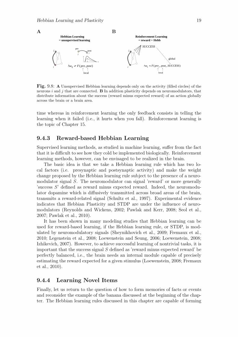
Fig. 9.8: A Unsupervised Hebbian learning depends only on the activity (filled circles) of theneurons i and j that are connected. B In addition plasticity depends on neuromodulators, thatdistribute information about the success (reward minus expected reward) of an action globallyacross the brain or a brain area.

time whereas in reinforcement learning the only feedback consists in telling thelearning when it failed (i.e., it hurts when you fall). Reinforcement learning isthe topic of Chapter 15.

9.4.3 Reward-based Hebbian Learning

Supervised learning methods, as studied in machine learning, suffer from the factthat it is difficult to see how they cold be implemented biologically. Reinforcementlearning methods, however, can be envisaged to be realized in the brain.

The basic idea is that we take a Hebbian learning rule which has two lo-cal factors (i.e. presynaptic and postsynaptic activity) and make the weightchange proposed by the Hebbian learning rule subject to the presence of a neuro-modulator signal S. The neuromodulator can signal ’reward’ or more generally’success S’ defined as reward minus expected reward. Indeed, the neuromodu-lator dopamine which is diffusively transmitted across broad areas of the brain,transmits a reward-related signal (Schultz et al., 1997). Experimental evidenceindicates that Hebbian Plasticity and STDP are under the influence of neuro-modulators (Reynolds and Wickens, 2002; Pawlak and Kerr, 2008; Seol et al.,2007; Pawlak et al., 2010).

It has been shown in many modeling studies that Hebbian learning can beused for reward-based learning, if the Hebbian learning rule, or STDP, is mod-ulated by neuromodulatory signals (Sheynikhovich et al., 2009; Fremaux et al.,2010; Legenstein et al., 2008; Loewenstein and Seung, 2006; Loewenstein, 2008;Izhikevich, 2007). However, to achieve successful learning of nontrivial tasks, it isimportant that the success signal S defined as ’reward minus expected reward’ beperfectly balanced, i.e., the brain needs an internal module capable of preciselyestimating the reward expected for a given stimulus (Loewenstein, 2008; Fremauxet al., 2010).

9.4.4 Learning Novel Items

Finally, let us return to the question of how to form memories of facts or eventsand reconsider the example of the banana discussed at the beginning of the chap-ter. The Hebbian learning rules discussed in this chapter are capable of forming


an internal memory trace of the banana, but they will also form memory tracesof everything else we see or feel or think: our direction of gaze changes two orthree times per second so that even during a single day more than a hundredthousand perceived images would have to be stored. It can be shown that such acontinued bombardment with sensory items leads to rapid overwriting of memo-ries, with the result that what we have memorized earlier is quickly washed outand forgotten (Fusi, 2002). In order to make memory storage and retrieval sta-ble, one needs to postulate a gating mechanism which decides which perceptionis novel or interesting and worth storing. Similar to the situation discussed forreward-based Hebbian learning, neuromodulators could play the role of global,brain-wide gating signal (Pawlak et al., 2010) Hebbian learning of a synapse fromneuron j to i depends then not only on the activities of those two neurons, butalso on the presence of a more global neuromodulator that enables the initiationor stabilization of Hebbian weight changes (Hasselmo, 1999; Clopath et al., 2008;Frey and Morris, 1998). The topics sketched here in the last few paragraphswill be discussed in greater depth in Chapter 15 (Reinforcement Learning) andChapter 9 (Neuromodulation).

9.5 Core Set of Readings:

a) Spiking Neuron Models, by W. Gerstner and W. Kistler, chapters 10-12 (Cam-bridge Univ. Press, 2002)

b) Theory of Cortical Plasticity by L.N. Cooper, N. Intrator, B.S. Blais andH.Z. Shouval, (World Scientific, 2004)

c) Timing is not everything: neuromodulation opens the STDP gate, V.Pawlak and J.R. Wickens and A. Kirkwood and J.N.D. Kerr, Front. SynapticNeurosci. (2010)

d) J. Sjostrom and W. Gerstner, Spike-Timing Dependent Plasticity, Schol-arpedia (2010)


9.6 Exercises

Exercise 1:Assume that plasticity is controlled by the learning rule (9.8) with a parameter

θ = 20Hz. The postsynaptic neuron is described as a rate neuron with firing rateνi = g(

∑j wijνj). For the sake of simplicity we assume that g is linear, i.e.

g(x) = x. All synaptic weights and firing rates are positive.a) Consider a single presynaptic neuron j that is connected with a weight wij

to the postsynaptic neuron. Show that the postsynaptic rate has a fixed point atνi = θ.

b) Show that this fixed point is unstable.c) Suppose that there are 20 presynaptic neurons. The input alternates between

two patterns. In the first pattern, the first half of neurons 1 ≤ j ≤ 10 fires ata rate of νj = 1Hz while the other presynaptic neurons are silent. In the secondpattern, the first half of neurons is silent while the other neurons 11 ≤ j ≤ 20 fireat a rate of νj = 3Hz. The input switches several times back and forth between thetwo patterns. Suppose that initially all weights have the same value wij = 1. Howdo the weights evolve in the presence of the sequence of input patterns? Allow forhard bounds at wij = 0 and wij = 2

d) As in c, but suppose that during the first pattern the first group fires at2.5Hz. What happens?

Exercise 2.All eigenvectors of the correlation matrix are fixed points under Oja’s learning

rule. Show that only the eigenvector corresponding to the largest eigenvalue isstable.

To do so, assume that the current weight vector is close to eigenvector ~ei, buthas a small perturbation in the direction of ~ej. Hence, write

~w = ~ei + c~ej where |c| � 1 is the amplitude of the perturbation and analyzewhether the perturbation grows or decays.

Exercise 3.a) Derive the exponential learning window (9.21) assuming four substances

with concentrations [a], [b], [c], [d] and time constants τa, τb, τc, τd respectively anddynamics analogous to (9.23), where τc is a second presynaptic process and τd afurther postsynaptic process. To do so, take the limit τb → 0 and τc → 0.

b) What happens if you do not take the two limits, but keep τb and τc in therange of a few milliseconds. Show that the resulting learning window is a smoothfunction that does not necessarily go through the origin.

Bibliography

Abbott, L. F. and Nelson, S. B. (2000). Synaptic plastictiy - taming the beast. NatureNeuroscience, 3:1178–1183.

Abbott, L. F., Varela, J. A., Sen, K., and Nelson, S. B. (1997). Synaptic depressionand cortical gain control. Science, 275:220–224.

Artola, A., Brocher, S., and Singer, W. (1990). Different voltage dependent thresholdsfor inducing long-term depression and long-term potentiation in slices of rat visualcortex. Nature, 347:69–72.

Bi, G. and Poo, M. (1998). Synaptic modifications in cultured hippocampal neurons:dependence on spike timing, synaptic strength, and postsynaptic cell type. J. Neu-rosci., 18:10464–10472.

Bienenstock, E., Cooper, L., and Munroe, P. (1982). Theory of the development ofneuron selectivity: orientation specificity and binocular interaction in visual cortex.J. Neurosci., 2:32–48.

Buonomano, D. and Merzenich, M. (1998). Cortical plasticity: From synapses to maps.Annual Review of Neuroscience, 21:149–186.

Caporale, N. and Dan, Y. (2008). Spike timing-dependent plasticity: A hebbian learn-ing rule. Ann. Rev. Neurosci., 31:25–46.

Clopath, C., Busing, L., Vasilaki, E., and Gerstner, W. (2010). Connectivity reflectscoding: A model of voltage-based spike-timing-dependent-plasticity with homeosta-sis. Nature Neuroscience, 13:344–352.

Clopath, C., Ziegler, L., Vasilaki, E., Busing, L., and Gerstner, W. (2008). Tag-trigger-consolidation: A model of early and late long-term-potentiation and depression.PLOS Comput. Biol., 4:e1000248.

Fremaux, N., Sprekeler, H., and Gerstner, W. (2010). Functional requirements forreward-modulated spike-timing-dependent plasticity,. J. Neurosci., 40:13326–13337.

Frey, U. and Morris, R. (1998). Synaptic tagging: implications for late maintenance ofhippocampal long-term potentiation. Trends in Neurosciences, 21:181–188.

Fusi, S. (2002). Hebbian spike-driven synaptic plasticity for learning patterns of meanfiring rates. Biol. Cybern., 87:459–470.

Gerstner, W., Kempter, R., van Hemmen, J., and Wagner, H. (1996). A neuronallearning rule for sub-millisecond temporal coding. Nature, 383(6595):76–78.

23


Gerstner, W. and Kistler, W. K. (2002). Spiking Neuron ModelsL single neurons,populations, plasticity. Cambridge University Press, Cambridge UK.

Hasselmo, M. (1999). Neuromodulation: acetylcholine and memory consolidation.Trends in Cognitive Sciences, 3:351–359.

Hebb, D. O. (1949). The Organization of Behavior. Wiley, New York.

Izhikevich, E. (2007). Solving the distal reward problem through linkage of stdp anddopamine signaling. Cerebral Cortex, 17:2443–2452.

Legenstein, R., Pecevski, D., and Maass, W. (2008). A learning theory for reward-modulated spike-timing-dependent plasticity with application to biofeedback. PLOSComput. Biol., 4:e1000180.

Lisman, J. and Zhabotinsky, A. (2001). A model of synaptic memory: A CaMKII/PP1switch that potentiates transmission by organizing an AMPA receptor anchoringassembly. Neuron, 31:191–201.

Loewenstein, Y. (2008). Robustness of learning that is based on covariance-drivensynaptic plasticity. PLOS Comput. Biol., 4:e1000007.

Loewenstein, Y. and Seung, H. (2006). Operant matching is a generic outcome ofsynaptic plasticity based on the covariance between reward and neural activity. Proc.Natl. Acad. Sci. USA, 103:15224–15229.

MacKay, D. J. C. and Miller, K. D. (1990). Analysis of linsker’s application of hebbianrules to linear networks. Network, 1:257–297.

Makram, H., Sjostrom, J., and Gerstner, W. (2011). A history of spike-timing depen-dent plasticity. Frontiers in Synaptic Neuroscience, xx:xx.

Markram, H., Lubke, J., Frotscher, M., and Sakmann, B. (1997). Regulation of synapticefficacy by coincidence of postysnaptic AP and EPSP. Science, 275:213–215.

Markram, H., Wu, Y., and Tosdyks, M. (1998). Differential signaling via the same axonof neocortical pyramidal neurons. Proc. Natl. Acad. Sci. USA, 95:5323–5328.

Miller, K. D. and MacKay, D. J. C. (1994). The role of constraints in hebbian learning.Neural Computation, 6:100–126.

Ngezahayo, A., Schachner, M., and Artola, A. (2000). Synaptic activation modulatesthe induction of bidirectional synaptic changes in adult mouse hippocamus. J. Neu-roscience, 20:2451–2458.

Oja, E. (1982). A simplified neuron model as a principal component analyzer. J.Mathematical Biology, 15:267–273.

Pawlak, V. and Kerr, J. (2008). Dopamine receptor activation is required for corticos-triatal spike-timing-dependent plasticity. J. Neuroscience, 28:2435–2446.

Pawlak, V., Wickens, J., Kirkwood, A., and Kerr, J. (2010). Timing is not everything:neuromodulation opens the stdp gate. Front. Synaptic Neurosci., 2:146.

Pfister, J.-P. and Gerstner, W. (2006). Triplets of spikes in a model of spike timing-dependent plasticity. J. Neuroscience, 26:9673–9682.


Recanzone, G. H., Schreiner, C. E., and Merzenich, M. M. (1993). Plasticity in thefrequency representation of primary auditory cortex following discrimination trainingin adult owl monkeys. The Journal of Neuroscience, 13:87–103.

Reynolds, J. and Wickens, J. (2002). Dopamine-dependent plasticity of corticostriatalsynapses. Neural Networks, 15:507–521.

Rubin, J., Gerkin, R., Bi, G.-Q., and Chow, C. (2005). Calcium time course as a signalfor spike-timing-dependent plasticity. J. Neurophysiology, 93:2600–2613.

Schultz, W., Dayan, P., and Montague, R. (1997). A neural substrate for predictionand reward. Science, 275:1593–1599.

Senn, W., Tsodyks, M., and Markram, H. (2001). An algorithm for modifying neuro-transmitter release probability based on pre- and postsynaptic spike timing. NeuralComputation, 13:35–67.

Seol, G., Ziburkus, J., Huang, S., Song, L., Kim, I., Takamiya, K., Huganir, R., Lee,H.-K., and Kirkwood, A. (2007). Neuromodulators control the polarity of spike-timing-dependent synaptic plasticity. Neuron, 55:919–929.

Sheynikhovich, D., Chavarriaga, R., Strosslin, T., Arleo, A., and Gerstner, W. (2009).Is there a geometric module for spatial orientation? insights from a rodent navigationmodel. Psychological Review, 116:540–566.

Shouval, H. Z., Bear, M. F., and Cooper, L. N. (2002). A unified model of nmdareceptor dependent bidirectional synaptic plasticity. Proc. Natl. Acad. Sci. USA,99:10831–10836.

Sjostrom, P., Turrigiano, G., and Nelson, S. (2001). Rate, timing, and cooperativityjointly determine cortical synaptic plasticity. Neuron, 32:1149–1164.

Wimbauer, S., Gerstner, W., and van Hemmen, J. (1998). Analysis of a correlation-based model for the development of orientation-selective receptive fields in the visualcortex. Network, 9:449–466.

0 hebbian learning and plasticity - semantic scholar · 0 hebbian learning and plasticity ... from...

Documents