Principal Component Analysisbased on: Neural networks: a comprehensive foundation

by Simon Haykin

1

1 - The Hebbian Learning

• Hebb’s postulate of learning is the oldest and most famous of

all learning rules; it is named in honor of neuropsychologist

Hebb (1949).

• The Organization of Behaviour (1949): When an axon of cell

A is near enough to excite a cell B and repeatedly or

persistently takes part in firing it, some growth process or

metabolic changes take place in one or both cells such that

A’s efficiency as one of the cells firing B, is increased.

• Hebb proposed this change as a basis of associative learning

(at the cellular level), which would result in an enduring

modification in the activity pattern of a spatially distributed

assembly of nerve cells.

• This statement is made in a neurobiological context. We can

restate it as:

2

1. If two neurons on either side of a synapse are activated

simultaneously (i.e. synchronously), then the strength of

that synapse is selectively increased.

2. If two neurons on either side of a synapse are activated

asynchronously, then that synapse is selectively weakened

or eliminated.

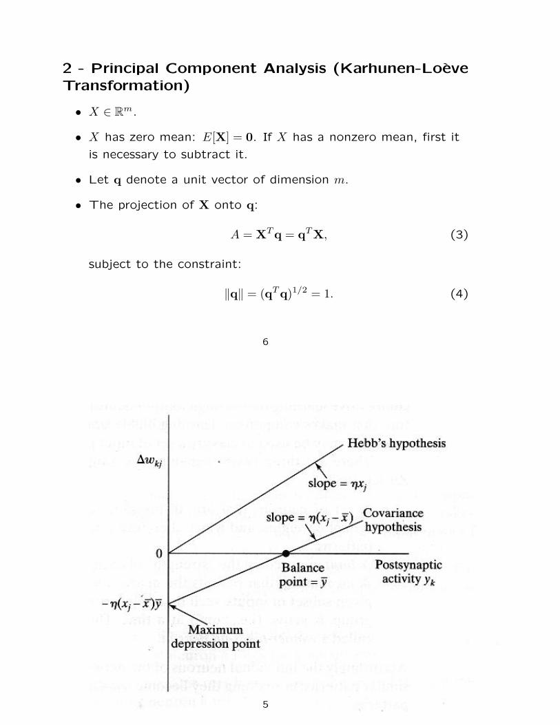
• The Hebb’s hypothesis:

∆wkj(n) = ηyk(n)xj(n), (1)

where η is the learning rate. However, this leads to exponential

growth which is physically unacceptable.

• In order, to overcome this Sejnowsky (1977) introduced the

covariance hypothesis:

∆wkj = η(xj − x)(yk − y). (2)

In this situation, wkj can increase or decrease.

3

• Both learning rules are ilustrated in the following Figure.

4

5

2 - Principal Component Analysis (Karhunen-Loeve

Transformation)

• X ∈ Rm.

• X has zero mean: E[X] = 0. If X has a nonzero mean, first it

is necessary to subtract it.

• Let q denote a unit vector of dimension m.

• The projection of X onto q:

A = XT q = qT X, (3)

subject to the constraint:

‖q‖ = (qT q)1/2 = 1. (4)

6

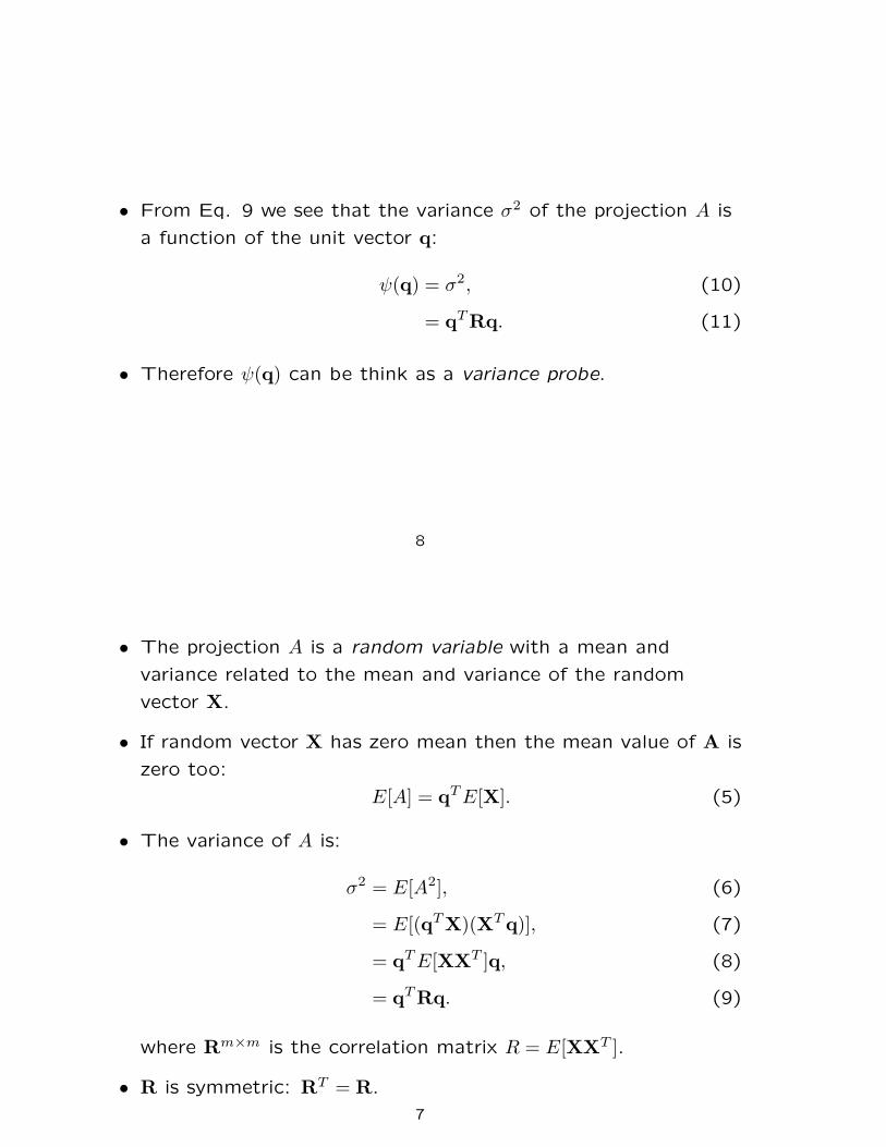
• The projection A is a random variable with a mean and

variance related to the mean and variance of the random

vector X.

• If random vector X has zero mean then the mean value of A is

zero too:

E[A] = qTE[X]. (5)

• The variance of A is:

σ2 = E[A2], (6)

= E[(qTX)(XT q)], (7)

= qTE[XXT ]q, (8)

= qT Rq. (9)

where Rm×m is the correlation matrix R = E[XXT ].

• R is symmetric: RT = R.

7

• From Eq. 9 we see that the variance σ2 of the projection A is

a function of the unit vector q:

ψ(q) = σ2, (10)

= qT Rq. (11)

• Therefore ψ(q) can be think as a variance probe.

8

3 - Eigenstructure of Principal Component Analysis

• We want to find those unit vectors q along which ψ(q) has

extremal values (local maxima or minima), subject to a

constraint on the Euclidean norm of q.

• The solution of this problem lies can be expressed by:

Rq = λq, (12)

which is the equation of the eigenstructure of the correlation

matrix R.

• Let the eigenvalues of Rm×m be denoted by λ1, λ2, . . . , λm and

the associated eigenvectors be denoted by q1,q2, . . . ,qm:

Rqj = λjqj j = 1, . . . ,m. (13)

• Let the corresponding eigenvalues be arranged in decreasing

order:

λ1 > λ2 > . . . > λj > . . . > λm,

9

so that λ1 = λmax.

• Let the associated eigenvectors be used to construct the

following matrix:

Q = [q1,q2, . . . ,qj , . . . ,qm] . (14)

• We may then combine the set of m equations of Eq. 13 into a

single equation:

RQ = QΛ, (15)

where Λ is a diagonal matrix defined by:

Λ = diag [λ1, λ2, . . . , λj , . . . , λm] (16)

• Q is an orthogonal matrix:

qTi qj =

1, j = i

0, j 6= i. (17)

10

• we may write:

QT Q = I, (18)

or:

QT = Q−1. (19)

• We may rewrite Eq. 15 as the orthogonal Similarity

transformation:

QT RQ = Λ. (20)

Or in a expanded form:

qTj Rqk =

λj , k = j

0, k 6= j.(21)

• The correlation matrix R may be itself be expressed in terms

of its eigenvalues and eigenvectors as:

R =m

∑

i=1

λiqiqTi . (22)

11

• Principal component analysis and eigendecomposition of

matrix R are basically the same thing.

• Variance probes and eigenvalues are equal:

ψ(qj) = λj , j = 1, 2, . . . ,m. (23)

12

• Let the data vector x denote a realisation of the random

vector X.

• The projection of x onto qj can be written like:

aj = qTj x = xT qj , j = 1, 2, . . . ,m. (24)

• The aj are called the principal components.

• The reconstruction:

a = [a1, a2, . . . , am]T , (25)

=[

xT q2,xTq2,x

Tqm

]T, (26)

= QT x. (27)

x = Qa (28)

=m

∑

j=1

ajqj . (29)

13

4 - Dimensionality Reduction

• PCA provides an effective technique for dimensionality

reduction.

• Let λ1, λ2, . . . , λl denote the largest eigenvalues of the

correlation matrix R.

• The data vector x can be aproximated by truncating the

expansion of:

x = QT a =m

∑

j=1

ajqj , (30)

14

after l terms as follows:

x =l

∑

j=1

ajqj , (31)

= [q1,q2, . . . ,ql]

a1

a2

...

al

, l ≤ m (32)

• Given the original data vector x it is possible to calculate the

set of principal components a as follows:

a1

a2

...

al

=

qT1

qT2

...

qTl

x, l ≤ m (33)

15

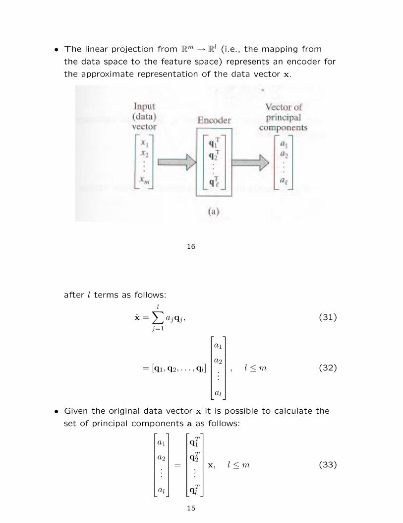
• The linear projection from Rm → R

l (i.e., the mapping from

the data space to the feature space) represents an encoder for

the approximate representation of the data vector x.

16

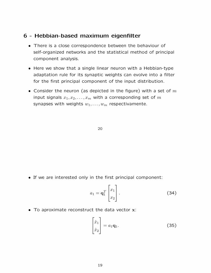
• The linear projection from Rl → R

m represents a decoder for

the approximate reconstruction of the original data vector x.

17

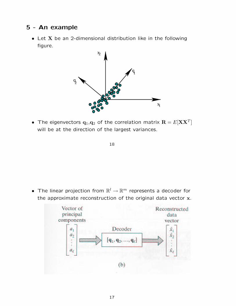
5 - An example

• Let X be an 2-dimensional distribution like in the following

figure.

x2

x1

q2

q1

• The eigenvectors q1,q2 of the correlation matrix R = E[XXT ]

will be at the direction of the largest variances.

18

• If we are interested only in the first principal component:

a1 = qT1

x1

x2

. (34)

• To aproximate reconstruct the data vector x:

x1

x2

= a1q1. (35)

19

6 - Hebbian-based maximum eigenfilter

• There is a close correspondence between the behaviour of

self-organized networks and the statistical method of principal

component analysis.

• Here we show that a single linear neuron with a Hebbian-type

adaptation rule for its synaptic weights can evolve into a filter

for the first principal component of the input distribution.

• Consider the neuron (as depicted in the figure) with a set of m

input signals x1, x2, . . . , xm with a corresponding set of m

synapses with weights w1, . . . , wm respectivamente.

20

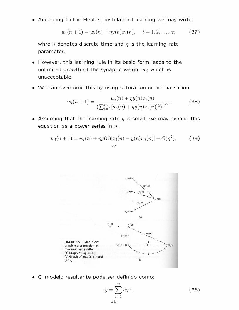
• O modelo resultante pode ser definido como:

y =

m∑

i=1

wixi (36)

21

• According to the Hebb’s postulate of learning we may write:

wi(n+ 1) = wi(n) + ηy(n)xi(n), i = 1, 2, . . . ,m, (37)

whre n denotes discrete time and η is the learning rate

parameter.

• However, this learning rule in its basic form leads to the

unlimited growth of the synaptic weight wi which is

unacceptable.

• We can overcome this by using saturation or normalisation:

wi(n+ 1) =wi(n) + ηy(n)xi(n)

(∑m

i=1[wi(n) + ηy(n)xi(n)]2)

1/2. (38)

• Assuming that the learning rate η is small, we may expand this

equation as a power series in η:

wi(n+ 1) = wi(n) + ηy(n)[xi(n) − y(n)wi(n)] +O(η2), (39)

22

where the term O(η2) represents second and highest order

effects in η. For small η we can ignore it and write:

wi(n+ 1) = wi(n) + ηy(n)[xi(n) − y(n)wi(n)]. (40)

• y(n)xi(n) is the usual Hebbian rule and the term −y(n)wi(n) is

the negative feedback.

• We might rewrite the learning rule as:

wi(n+ 1) = wi(n) + ηy(n)x′i(n), (41)

where:

x′i(n) = xi(n) − y(n)wi(n). (42)

• A matrix formulation might be written as:

w(n+ 1) = w(n) + η[

x(n)xT w(n) −wT (n)x(n)xT (n)w(n)]

(43)

23

7 - Properties of the Hebbian-Based Maximum

Eigenfilter

1. The variance of the model output approches the largest

eigenvalue of the correlation matrix:

limn→∞

σ2(n) = λ1. (44)

2. The synaptic weight vector of the model approaches the

associated eigenvector, as shown by:

limn→∞

w(n) = q1, (45)

with

limn→∞

‖w(n)‖ = 1. (46)

24

8 - Hebbian-Based Principal Component Analysis

• The Hebbian based maximum eigenfilter extracts only the first

principal component of the input.

• However this can be expanded to extract the first l principal

components as ilustrated in the following Figure.

• The learning algorithm could be summarised as:

1. Initialise the synaptic weights of the network, wji, to small

random values at time n = 1. Assign a small learning rate

parameter η.25

2. For n = 1, j = 1, 2, . . . , l and i = 1, 2, . . . ,m compute:

yj(n) =

m∑

i=1

wji(n)xi(n), (47)

∆wji(n) == η

[

yj(n)xi(n) − yj(n)

j∑

k=1

wki(n)yk(n)

]

, (48)

where xi(n) is the i-th component of the m-by-1 input

vector x(n) and l is the desired number of components.

3. Increment n by 1, go to Step 2, and continue until the

synaptic weights wji reach their steady state values.

26

9 - An example: image coding (1)

1. Fig. a-) Original image with 256x256 pixels, 256 gray levels.

2. The image was coded using a linear feedforward network with

a single layer of 8 neurons each with 64 inputs.

3. To train the network 8x8 nonoverlapping blocks of the image

were used.

4. The experiment was performed with 2000 scans of the picture

and a small learning rate η = 10−4.

5. Fig. b-) shows the 8x8 masks representing the synaptic

weights learned by the network. Excitatory (positive) synapses

are white, inhibitory (negative) synapses are black, gray

indicates zero weights.

6. Fig. c-) shows the reconstruction using the dominant 8

principal components.

27

7. Fig. d-) Each coefficient was uniformly quantized with a

number of bits approximately proportionally to the logarithm of

the variance of that coefficient over the image. Thus the first

three masks were assigned 6 bits, th next two masks 4 bits

each, the next two masks 3 bits each, and the last mask 2bits.

Based on this representation a total of 34 bits were needed to

code each 8x8 block of pixels, resulting in a data rate of 0.53

bits per pixel. This results in a compression of 15:1.

28

29

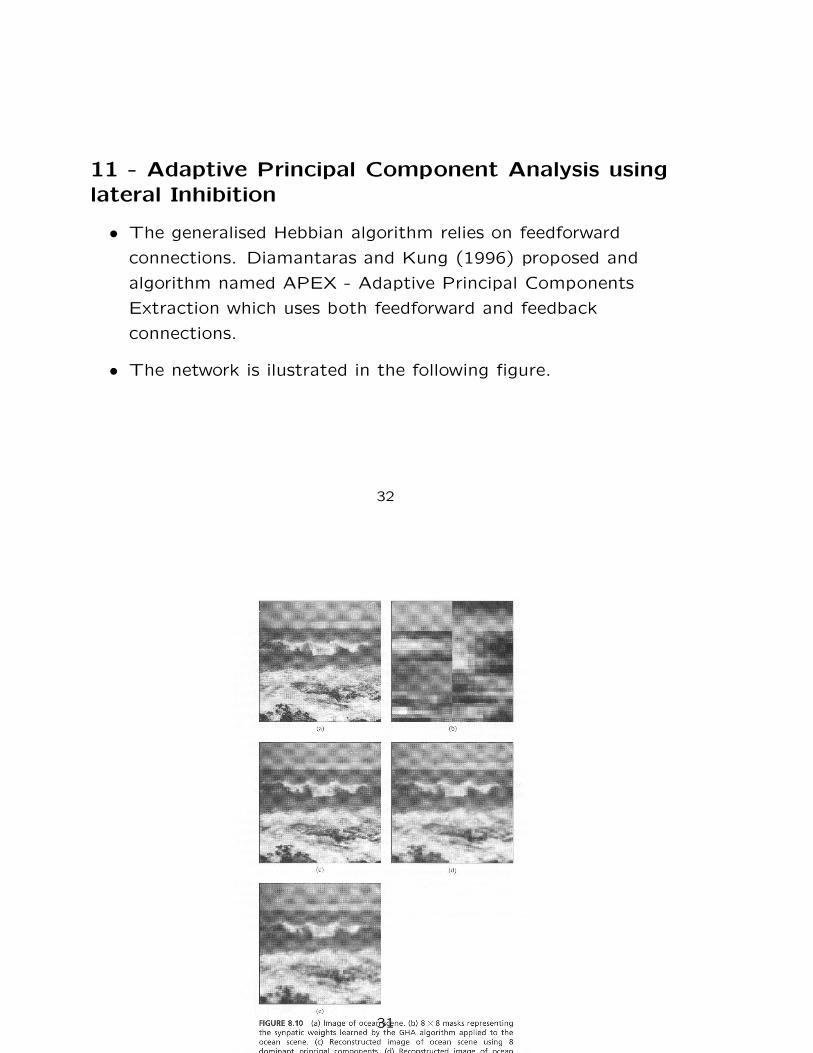
10 - An example: image coding (2)

1. Fig. a-) Original image with 256x256 pixels, 256 gray levels.

2. The image was coded using a linear feedforward network with

a single layer of 8 neurons each with 64 inputs.

3. Fig. b-) shows the 8x8 masks representing the synaptic

weights learned by the network. Excitatory (positive) synapses

are white, inhibitory (negative) synapses are black, gray

indicates zero weights.

4. Fig. c-) shows the reconstruction using the dominant 8

principal components.

5. Fig. d-) Reconstruction with compression ratio of 22:1.

6. Fig. e-) Reconstruction using principal components of example

1 ans 22:1 compression ratio.

30

31

11 - Adaptive Principal Component Analysis using

lateral Inhibition

• The generalised Hebbian algorithm relies on feedforward

connections. Diamantaras and Kung (1996) proposed and

algorithm named APEX - Adaptive Principal Components

Extraction which uses both feedforward and feedback

connections.

• The network is ilustrated in the following figure.

32

where the feedforward connections are:

wj = [wj1, wj2, . . . , wjm] . (49)

33

and the lateral connections are:

aj = [aj1, aj2, . . . , ajj−1]T

(50)

• The algorithm can be summarised as:

1. Initialise wj and aj to small random values at time n = 1

where j = 1, 2, . . . ,m. assign a small positive value to η.

2. set j = 1 and for n = 1, 2, . . . compute

y1(n) = wT1(n)x(n), (51)

w1 = w1(n) = η[y1(n)x(n) − y2

1(n)w1(n)]. (52)

3. Set j = 2 and for n = 1, 2, . . . compute:

yj−1(n) = [y1(n), . . . , yj−1(n)]T (53)

yj(n) = wTj (n)x(n) + aT

j (n)yj−1(n) (54)

wj(n+ 1) = wj(n) + η[yj(n)x(n) − y2

j (n)wj(n)] (55)

aj(n+ 1) = aj(n) − η[yj(n)yj−1(n) + y2

j (n)aj(n)] (56)

34

4. Increment j by 1 go to Step 3 and contiue until j = m,

where m is the desired number of principal components.

35