0 0 01 80 for pdf - michigan state university

AQUIFER CHARACTERIZATION

Edited by:

JOHN S. BRIDGEDepartment of Geological Sciences, Binghamton University

Binghamton, New York 13902-6000, U.S.A.AND

DAVID W. HYNDMANDepartment of Geological Sciences, Michigan State University, 206 Natural Science Building,

East Lansing, Michigan 48824-1115, U.S.A.

Copyright 2004 bySEPM (Society for Sedimentary Geology)

Laura J. Crossey, Editor of Special PublicationsSEPM Special Publication Number 80

Tulsa, Oklahoma, U.S.A. August, 2004

ISBN 1-56576-107-3

© 2004 bySEPM (Society for Sedimentary Geology)

6128 E. 38th Street, Suite 308Tulsa, OK 74135-5814, U.S.A.

Printed in the United States of America

SEPM and the authors are grateful to the followingfor their generous contribution to the cost of publishing

Aquifer Characterization

Contributions were applied to the cost of production, which reduced thepurchase price, making the volume available to a wide audience

Emporia State University, Hydrogeology Program

INEEL Laboratory Directed Research & Development Programunder DOE Idaho Operations Office Contract DE-AC07-99ID13727

Institute of Environmental Science and Research (ESR), New Zealand

Kansas Geological Survey

Michigan State University

National Science Foundation Project no. 0208492

SEPM (Society for Sedimentary Geology) is an international not-for-profit Society based in Tulsa,Oklahoma. Through its network of international members, the Society is dedicated to the disseminationof scientific information on sedimentology, stratigraphy, paleontology, environmental sciences, marinegeology, hydrogeology, and many additional related specialties.

The Society supports members in their professional objectives by publication of two major scientific journals, theJournal of Sedimentary Research (JSR) and PALAIOS, in addition to producing technical conferences, short courses,and Special Publications. Through SEPM's Continuing Education, Publications, Meetings, and other programs,members can both gain and exchange information pertinent to their geologic specialties.

For more information about SEPM, please visit www.sepm.org.

3INTEGRATION OF SEDIMENTOLOGIC AND HYDROGEOLOGIC PROPERTIES

INTEGRATION OF SEDIMENTOLOGIC AND HYDROGEOLOGICPROPERTIES FOR IMPROVED TRANSPORT SIMULATIONS

SUSANNE E. BITEMAN, DAVID W. HYNDMAN, M.S. PHANIKUMAR, AND GARY S. WEISSMANNDepartment of Geological Sciences, Michigan State University, 206 Natural Science Building,

East Lansing, Michigan 48824-1115, U.S.A.e-mail: [email protected]; [email protected]; [email protected]

ABSTRACT: Traditional geostatistical approaches for estimating distributions of hydraulic conductivity fail to reflect sharp contrasts thatoccur at boundaries between different stratigraphic units, thus limiting the accuracy of contaminant-transport models. We present anapproach to incorporate a stratigraphic framework into geostatistical simulation at the scale of a plume, to better represent aquiferheterogeneity. The approach was developed and tested at the Schoolcraft Bioremediation Site in southwestern Michigan, where detailedestimates of aquifer properties were needed to accurately simulate multi-component reactive transport and to design an effectivebioremediation strategy. The sediments at the site were deposited as glaciofluvial outwash downstream of the Kalamazoo Moraine, andconsist mainly of fine to medium sands with interbedded gravels and silts. A series of 18-meter-long continuous cores was collected inthe vicinity of the bioremediation-system delivery wells. These cores were assessed for sedimentary facies, grain-size distribution,porosity, and hydraulic conductivity. Sedimentologic measurements from outcrop analogs supplemented the core data from the site.On the basis of the core data, the aquifer was separated into four stratigraphic units, and the measured conductivity values weregeostatistically interpolated within each stratigraphic unit. The stratigraphically based estimates of hydraulic conductivity were usedas input to a high-resolution, three-dimensional model of groundwater flow and solute transport in the region. The model withstratigraphic interpolation provided better transport predictions for an injected tracer pulse than models that do not incorporate thestratigraphy.

Aquifer CharacterizationSEPM Special Publication No. 80, Copyright © 2004SEPM (Society for Sedimentary Geology), ISBN 1-56576-107-3, p. 3–13.

INTRODUCTION

Accurate predictions of solute transport are commonly lim-ited by the ability to preserve sharp gradients in aquifer param-eters, yet these sharp gradients may be identified using aquiferstratigraphic analysis. Over the past few decades, several work-ers have shown that heterogeneity in hydraulic conductivity (K)and other aquifer parameters (e.g., porosity and storage coeffi-cients) are controlled largely by the distribution of sedimentarymaterial in the aquifer (e.g., Fogg, 1989; Anderson, 1989; Webband Anderson, 1996; Davis et al., 1997; Webb and Davis, 1998;Anderson et al., 1999; Bersezio et al., 1999; Hornung and Aigner,1999; Klingbeil et al., 1999; Ritzi et al., 2000).

The statistics of aquifer parameters also commonly vary sig-nificantly between different stratigraphic units (Davis et al., 1997;Carle et al., 1998; Ritzi et al., 2000). Thus, when using geostatisticsto estimate aquifer parameters, variogram correlation lengthsshould be independently evaluated for each stratigraphic zone ifthe necessary data are available from either core measurementsor outcrop analog studies. The mean and variance of aquiferparameters, such as hydraulic conductivity, also vary by strati-graphic unit and thus are not globally stationary. Geostatisticalmethods, from kriging to stochastic simulation, can be used moreeffectively to estimate aquifer parameters using differentvariogram models for each stratigraphic zone.

Eschard et al. (1998) and Weissmann and Fogg (1999) used thegeology and stratigraphy as a framework for geostatistical real-izations to avoid the assumption of global stationarity of theaquifer parameter statistics. Rather than assuming that the mean,variance, and correlation lengths are stationary across the entirearea of geostatistical inference, such approaches have a lessrestrictive assumption that these statistics are stationary onlyacross an individual geologic unit. These approaches were ap-plied at the regional scale; however, point-source remediationtypically requires that models of heterogeneity be developed atthe smaller, plume scale.

In this paper, we present a modification of the stratigraphi-cally based approach of Eschard et al. (1998) and Weissmann andFogg (1999) to interpolate measured hydraulic conductivity at aplume scale. Our results show that incorporation of geologicinformation in the form of identified stratigraphic zonation im-proved our ability to predict tracer transport through aglaciofluvial aquifer in southeastern Michigan.

SITE DESCRIPTION

The Schoolcraft study site is located southeast of Schoolcraft,Michigan, on the glaciofluvial outwash plain associated with theKalamazoo Moraine (Fig. 1; Monaghan and Larson, 1982;Rheaume, 1990; Kehew et al., 1996). The Kalamazoo Moraine,located west of Kalamazoo, Michigan, and northwest of the studysite, was deposited when the Michigan Lobe ice margin stagnatedduring overall retreat of the Wisconsinan continental ice sheet(Monaghan and Larson, 1982).

Several contaminant plumes exist in the shallow glaciofluvialaquifer at Schoolcraft, Michigan (Hyndman et al. 2000; Dybas etal., 2002). The Schoolcraft Plume A study site (Fig. 2), the focus ofthis work, is located in an unconfined aquifer composed of a 27.5-m-thick succession of glaciofluvial sediments that lie directlyover a regionally extensive clay-rich till and lacustrine unit(Monaghan and Larson, 1982; Lipinski, 2002). This clay-rich unitacts as an aquitard in the Schoolcraft area (Lipinski, 2002). ThePlume A site is the location of a carbon tetrachloride (CT)bioaugmentation experiment, where microbes and substrate wereinjected to degrade aqueous and sorbed phase contaminants (Fig.2) (Hyndman et al., 2000; Dybas et al., 2002). This CT contaminantplume is about 1.2 km long and 90 m wide, extending fromroughly 8 to 26.5 m below ground surface (bgs), with CT concen-trations from 5 to 150 parts per billion (ppb). The water table atthis site lies at roughly 4.5 m bgs. Pilot studies indicated thatsediments above 8 m depth did not have CT contamination(Dybas et al., 1998); thus we have not included these shallow

S.E. BITEMAN, D.W. HYNDMAN, M.S. PHANIKUMAR, AND G.S. WEISSMANN4

kilometers0 10

- Kalamazoo River Valley (modern fluvial sediments)

- Climax-Scott Outwash Plain (older sands and

gravels)

- Outwash Plain (sands and gravels) related to

Kalamazoo Moraine

- Kalamazoo Moraine

- Till (clay-rich diamict)

Schoolcraft

Kalamazoo

Outcrop analog sites

FIG. 1.—Surficial geology of Kalamazoo County, Michigan. Also shown are the locations of the outcrop analog sites used in thisstudy. The modeling study area is located in the town of Schoolcraft. Modified from Monaghan and Larson (1982) andRheaume (1990).

FIG. 2.—The approximate distribution of Schoolcraft Plume A in the town of Schoolcraft (shown by roads). Our study site is at thelocation of the bioremediation project. Contours show the water-table elevation (in feet). Modified from Mayotte (1991).


sediments in this study. This biocurtain has proven to be greaterthan 97% effective at removing aqueous-phase contaminants(Hyndman, et al., 2000) and effective at removing sorbed-phaseCT in the biocurtain region over more than four years of operation(Dybas et al., 2002). The Schoolcraft Plume A site was chosen forthis study because a large database exists that includes coredescriptions, measurements of K from many wells, and manymeasured concentration histories collected during tracer tests.

The bioaugmentation system at this site consists of a series ofclosely spaced recirculation wells for delivery of microbes andnutrients (Fig. 3). Continuous core samples (approximately 5 cmin diameter) were collected from 7 of the 15 delivery well loca-tions and from 4 monitoring well locations (Fig. 3). Cores werecollected in sections 1.5 m long using the Waterloo continuouscore sampler, which advances a core barrel ahead of an augerstring. A vacuum-sealed core liner minimizes sample loss. Twenty-seven additional monitoring wells were drilled in both upgradientand downgradient locations relative to the biocurtain.

CORE ANALYSIS

Core samples were collected from wells D2, D4, D6, D8, D10,D12, D14, P6, P7, and P8 (Fig. 3; Table 1). These samples were cutinto 15.2 cm lengths, removed from the core liner, repacked totheir original volume in permeameter sleeves, flushed with car-bon dioxide gas, and tested for K using a constant-headpermeameter. The K measurements show that the highest Kvalues are generally located at the base of the aquifer and lowerK values are generally closer to the top of the aquifer (Fig. 4).Several discrete lenticular units of either low K or high K material,

FIG. 3.—Locations of delivery wells (D) and monitoring wells(MW or P) at the Plume A Schoolcraft Bioremediation site.

however, are present in the section. Preliminary modeling of flowand transport by Hoard (2002) indicated that the repacked Kmeasurements provided reasonable estimates of the actual hori-zontal K at the site, based on a reasonably good match betweensimulated and observed tracer concentration histories.

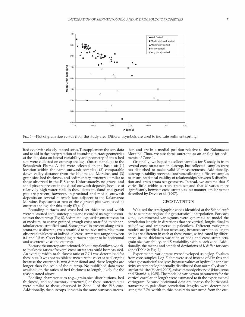
Grain-size distributions were measured for a subset of thesesamples using a standard sieve set (Table 1). The data show anexpected relationship between grain size, sorting, and K, wherecoarser-grained sediment tends to have higher K than fine-grainedsediment, and poor sorting reduces K (Fig. 5).

In order to gain additional insight into the aquifer stratigra-phy at the study site, core from well P18 and selected samplesfrom wells P6, P7, and P8 were analyzed for sedimentologiccharacteristics (e.g., grain-size distribution, vertical trends ingrain size, bedding thickness, and sedimentary structures) andvertical K of minimally disturbed sediment (Fig. 6). To assesssamples for vertical K, 42 subsamples (15.2 cm long) from the P18core were kept in the sampling tube, flushed with carbon dioxide,and tested for K using a constant-head permeameter. Resultsshow a trend in K similar to that observed in other wells, whererelatively high K values exist at the bottom of the aquifer andlower K values are found in the upper part of the aquifer (Fig. 6).

The measured vertical K values from core P18 were consis-tently lower than the repacked K measurements on samples of thesame grain size and zone from other wells by a factor of about0.74. Because repacked K values appear to reasonably representhorizontal K at the site (Hoard, 2002), we assume that this differ-ence represents the vertical to horizontal anisotropy in K. There-fore, the measured vertical K values from P18 were multiplied bythis ratio to develop horizontal K estimates for the interpolationto the groundwater model grid. Although it is possible that thisratio is biased by the fact that horizontal K values were allmeasured on repacked samples and all vertical samples weremeasured on intact core, it is generally expected that the verticalK will be lower than horizontal K because of a higher degree ofcontinuity of strata in the horizontal direction.

SITE STRATIGRAPHY

Four stratigraphic zones were identified in well P18 based onthe observed sedimentary character and K distribution (Figs. 6and 7). Stratigraphic boundaries were identified in cores usingone or more of the following characteristics: (1) an erosional basalcontact; (2) abrupt changes in mean grain size; and (3) abruptchanges in sedimentary structures and bedding thickness. Miss-ing core (from lack of recovery) created some uncertainty for zonedelineation. However, as is described in this section, detailedmeasurements of K and grain size (Fig. 4) provided additionalevidence of these stratigraphic boundaries across the modeledregion.

The basal zone, or Zone 1 (from ~ 27.5 m up to ~ 20.5 m depth),overlies the regional lacustrine clay or till and generally finesupward from cobbles in a coarse sand matrix up to medium sand.Though core was not collected across this boundary in well P18,cores from other wells indicate that this basal contact is erosionaland sharp. Drilling character and cuttings from P18 and otherwells indicate that the bottom one meter of this zone consistsmainly of cobbles. Sands in this zone are well sorted to poorlysorted with gravel. The sediment is cross-stratified, horizontallystratified, or massive. Because stratification may be too subtle torecognize in core, the massively bedded sands may actually bestratified. Gravel typically occurs along cross-strata in the sandybeds. Bedding thickness is difficult to determine in core becauseof the subtle nature of stratification. However, several cross-strata sets were distinguishable in this zone, being 0.1 to 0.25 m


thick. Measured K values through this zone are variable butconsistently higher than observed in other stratigraphic zones.Similar relatively high K deposits are observed in other wellsacross the site through this interval (Fig. 4).

Zone 2 (from ~ 20.5 to ~ 20.25 m depth in well P18) consists ofsilty sand to sandy silt with relatively low K over much of thestudy area. The sediments in the silty sand portion of this intervalare faintly laminated and display the lowest K of the stratigraphicsection. Though this zone is thin, it is distinctive because a low-Kfeature is recognized at this depth in a significant number of otherwells across the site (Fig. 4). As is described in the section ongroundwater modeling, delineation of this zone improved thetracer-test simulation results significantly.

Zone 3 (from ~ 20.25 to ~ 15.9 m depth) consists of fine tomedium sand that is moderately to well sorted. Beds in this zoneare typically cross-stratified to massive; however, the massivelybedded sands may have stratification that is too subtle to recog-nize in core. Grain size and sedimentary structures are morevariable in different cross-strata cosets than observed in eitherZone 1 or Zone 4. Additionally, set thickness is highly variable inthis zone, ranging from 0.05 to 0.25 m. Likewise, K in this zone ismore variable over short distances, with a mean intermediatebetween Zones 1 and 4 (Fig. 7). This mean and short-distancevariability in K is also observed across the study site, thus allow-ing delineation of this zone in other wells (Fig. 4).

Zone 4 (from about ~ 15.9 m to < 8 m depth) consists of wellsorted fine sand. A thin gravel lag was identified at the base ofthis zone. Individual beds appear to be relatively thin (0.05–0.15m) and cross-stratified or horizontally stratified, with massivebeds in places that may have stratification that is too subtle torecognize in core. K through this zone has low variability and islower than Zones 1 or 3 (Fig. 7). Similar consistently low-Kdistributions at this depth are observed in other wells at the site,thereby allowing delineation of this zone across the study area(Fig. 4).

The stratigraphic boundaries appear to be laterally continu-ous and horizontal at the scale of the study area. This is consistentwith observations at the outcrop analog sites, as is described inthe next section. This stratigraphic character is consistent withglaciofluvial outwash deposition of a retreating ice margin(Boothroyd and Ashley, 1975; Boothroyd and Nummedal, 1978;Maizels, 1995). The basal, coarse-grained unit (Zone 1) representsproximal to medial outwash deposited as the ice margin retreatedpast the Schoolcraft location. The upper zones (zones 2–4) most-likely represent distal outwash deposited when the ice marginstagnated at the Kalamazoo moraine.

OUTCROP ANALOG

Cores at the study site provide an excellent sampling ofvertical distributions for K analysis, but lateral data were lim-

Well Number

D2 D4 D6 D8 D10 D12 D14 P6 P7 P8 P18

Grain size 9 6 9 3 15 10 15 - - - 42

Repacked K 44 24 22 21 31 27 31 27 30 27 -

Vertical K - - - - - - - - - - 42

TABLE 1.—Number of samples analyzed from each well for grain size, repacked K, or vertical K.Dashes in cells indicate that no analysis was completed.

FIG. 4.—Plots showing the log-K data points used for interpola-tion and stratigraphic zonation. A) A transect through thedelivery wells (see Figure 3 for well locations). B) A transectthrough downgradient wells where K data were available.Zonal boundaries were identified at 16 m below groundsurface (bgs), 20 m bgs, and 21 m bgs. Modified from Hyndmanet al. (2000).


ited even with closely spaced cores. To supplement the core dataand to aid in the interpretation of bounding-surface geometriesat the site, data on lateral variability and geometry of cross-bedsets were collected on outcrop analogs. Outcrop analogs to theSchoolcraft Plume A site were selected on the basis of: (1)location within the same outwash complex, (2) comparabledown-valley distance from the Kalamazoo Moraine, and (3)grain size, bed thickness, and sedimentary structures similar tothose observed in the P18 core. Unfortunately, no gravel andsand pits are present in the distal outwash deposits, because ofrelatively high water table in these deposits. Sand and gravelpits are present, however, in proximal and medial outwashdeposits on several outwash fans adjacent to the KalamazooMoraine. Exposures at two of these gravel pits were used asoutcrop analogs for this study (Fig. 1).

Bounding surfaces and cross-bed set thickness and widthwere measured at the outcrop sites and recorded using photomo-saics of the outcrop (Fig. 8). Sediments exposed in outcrop consistof medium- to coarse-grained, trough cross-stratified to planar-tabular cross-stratified sand. Some gravel is present along cross-strata and as discrete, cross-stratified to massive units. Maximumobserved thickness of individual cross-strata sets range between0.1 and 0.5 m. Coset bounding surfaces appear to be horizontaland as extensive as the outcrop.

Because the outcrops are oriented oblique to paleoflow, width-to-thickness ratios of several cross-strata sets could be measured.An average width-to-thickness ratio of 7.7:1 was determined forthese sets. It was not possible to measure the coset or bed lengthsbecause the outcrop is two dimensional and these lengths arelonger than the scale of the outcrop. No published data wereavailable on the ratios of bed thickness to length, likely for thereason stated above.

Bedding characteristics (e.g., grain-size distributions, bedthickness, and sedimentary structures) at these outcrop siteswere similar to those observed in Zone 1 of the P18 core.Additionally, the outcrops lie within the same outwash succes-

sion and are in a medial position relative to the KalamazooMoraine. Thus, we use these outcrops as an analog for sedi-ments of Zone 1.

Originally, we hoped to collect samples for K analysis fromseveral cross-strata sets in outcrop, but collected samples weretoo disturbed to make valid K measurements. Additionally,outcrop instability prevented us from collecting sufficient samplesto ensure statistical validity of relationships between K distribu-tion and cross-strata set geometry. Instead, we assume that Kvaries little within a cross-strata set and that K varies moresignificantly between cross-strata sets in a manner similar to thatdescribed by Davis et al. (1997).

GEOSTATISTICS

We used the stratigraphic zones identified at the Schoolcraftsite to separate regions for geostatistical interpolation. For eachzone, experimental variograms were generated to model thecorrelation lengths in directions that are vertical, longitudinal topaleoflow, and transverse to paleoflow. Different variogrammodels are justified, if not necessary, because correlation lengthscales are different in each of these zones, as indicated by differ-ences in the thickness variation of beds and cross-strata sets,grain-size variability, and K variability within each zone. Addi-tionally, the means and standard deviations of K differ for eachzone (Table 2; Fig. 7).

Experimental variograms were developed using log-K valuesfrom core samples. Log-K data were used instead of K in this andother geostatistical analyses because values of hydraulic conduc-tivity were more log-normally distributed than normally distrib-uted at this site (Hoard, 2002), as is commonly observed (Hoeksemaand Kitanidis, 1985). The modeled variogram parameters for thevertical correlation length were estimated to fit the experimentalvariogram. Because horizontal data are sparse, the horizontal,transverse-to-paleoflow correlation lengths were determinedusing the 7.7:1 width-to-thickness ratio measured from the out-

FIG. 5.—Plot of grain size versus K for the study area. Different symbols are used to indicate sediment sorting.


FIG. 6.—Core description for well P18 showing zonal boundaries (marked by arrows) and measured vertical K. See Figure 3 forlocation.


crop analogs. Because outcrop analog data were not available inthe upper, distal outwash sediments (Zones 2, 3, and 4), todevelop lateral variograms in these units we assumed the samewidth-to-thickness ratio. Although this may add uncertainty tothe modeling, the effect on the final results is likely minimal.Sensitivity studies, however, may be conducted in future.

The horizontal, longitudinal-to-paleoflow correlation lengthswere extended as far as Groundwater Modeling System (GMS3.1,BYU, 2000) would allow, which is approximately 18 m. We believe

that this length is shorter than the true longitudinal-to-paleoflowcorrelation length based on the outcrop analogs and the nature ofthese fluvial deposits; however, the difference a slightly longervalue would make is likely insignificant. Table 3 summarizes thesill, nugget, longitudinal-to-flow range, transverse-to-flow range,and vertical range for each stratigraphic unit.

Using the estimated variogram models and conditioning Kdata from wells, we generated a three-dimensional log-K field foreach hydrostratigraphic zone using ordinary kriging. Thoughkriging may smooth results relative to conditional simulation, wechose kriging for this study because: (1) this approach mostclosely reflects current standard practice; (2) this allowed us todirectly compare these results to previously published modelingresults (e.g., Hyndman et al., 2000), and (3) the conditioning dataare very closely spaced, thus conditional simulation results wouldbe similar to kriging results in the region near the conductivitymeasurements. The kriging results from the four zones weremerged to create a final log-K field surrounding the biocurtainarea. This zonal kriged field preserved abrupt changes in K,especially noticeable at approximately 20–21 m depth in zone 2(Fig. 9A).

In addition to the zonal kriged results, a log-K field wasestimated by kriging without the zonal boundaries to evaluatethe influence of the additional geologic information (Fig. 9B).For this model, the variogram range was set at 18.0 m (to beconsistent with the zonal kriging). The nugget, sill, and range inall three orthogonal directions were fitted to the experimentalvariograms on the basis of core data (Table 3). In a visualcomparison, the zonal kriged field had significantly morehorizontal bedding-like features than the traditional krigedfield, which had smoother features with less horizontal conti-nuity. Additionally, the low-K region in Zone 2 is larger andmore diffuse in the nonzonal kriged case than suggested by thecore data (Fig. 9).

GROUNDWATER MODELING ANDTRACER-TEST SIMULATION

We used the three-dimensional groundwater flow model,MODFLOW-96 (McDonald and Harbaugh, 1988; Harbaughand McDonald, 1996), to predict hydraulic heads and ground-water fluxes for the region. Constant-head boundaries wereused in the flow direction to provide a gradient of 0.0011 basedon regional head measurements (Fig. 2). The model domain is arectangular region 101.5 m wide (y) by 57.2 m long (x) by 27.4 min depth (z). We discretized this region using a computationalgrid with 136 (y) x 86 (x) x 44 (z) cells. The delivery-well galleryis located at the center of the computational domain with finecells (20 cm x 20 cm) approximately equal to the size of theboreholes surrounding the delivery wells, and larger cells in ageometric progression away from the well gallery. The resolu-tion in the vertical direction varies and is discretized most finelyaround Zone 2 (Table 4).

During the tracer test, a conservative tracer (bromide) wasinjected into the seven even-numbered delivery wells and ex-tracted from the eight odd-numbered delivery wells for fivehours. During the next hour the same pumping rate was used ina flow-reversal phase in which tracer was extracted from theeven-numbered wells and injected into the odd-numbered wells.We used the reactive-transport code RT3D (Clement, 1997;Clement and Jones, 1998) to simulate three-dimensional tracertransport through the site. Because the concentration of injectedbromide changed during the tracer test, we divided the five-hour interval in the transport model into three stress periodswith different concentrations, 18, 14, and 17 ppm, respectively.

FIG. 7.—Box plots showing ranges of K for each stratigraphiczone. Each box shows the 25th, 50th (median), and 75th percen-tile of the population. The lines extending from the boxesshow the effective maxima and minima of the data popula-tion. Outliers (circles) are points that fall outside 1.5 times theinterquartile distance.

FIG. 8.—A portion of the outcrop analog for medial deposits (Zone1) at the Schoolcraft study site. A 40-cm-long shovel is shownfor scale.


The one-hour-flow-reversal phase was simulated with a singlestress period in which injected concentrations were 23.5 ppm.The last stress period in this simulation represents a 20-daynatural gradient period with no pumping. The differences inhydraulic conductivity across the vertical extent of the aquifercause proportional differences in the flux through differentlayers from the well. To represent this behavior, we used aconductivity-weighted average to compute the fluxes for theinjection and extraction wells.

RESULTS AND DISCUSSION

The tracer-test comparison shows that the addition of geo-logic data significantly improved transport simulations in someregions whereas in others the zonal and nonzonal simulatedtracers are similar (Fig. 10). In many cases, the hydrostratigraphicinterpretation improves the match between simulated and ob-served tracer concentrations, whereas in a few cases it reducedthe match slightly. Overall, the zonal model reduced the sum ofsquared residuals from 13.24 to 10.47, or roughly a 21% improve-ment. These residuals are calculated using the normalized con-centrations (from 0 to 1); thus, squaring these residuals withvalues < 1 provides a conservative estimate of the improvementmade by including the geologic information.

The largest difference between the zonal kriging model andthe nonzonal model was the preservation of the abrupt natureof contacts between Zones 1, 2, and 3 in the zonal model. Themost significant improvement in the tracer simulation was alsoin the region around Zone 2 (at 19.8 m depth), especially at wellsMW10 and MW13, where the low-K silty fine sand was observedacross more than half of the delivery-well area. The core de-scriptions and K data indicate that this unit extends throughdelivery wells D8, D10, and D12. MW13 and MW10 are locateddowngradient from delivery wells D10 and D8, respectively(Fig. 3). At the same depth in MW11 and MW12 there is noevidence for the low-K silty fine sand in Zone 2, and the simu-lations of tracer concentration respond similarly for both types

of kriging for these wells. No core was recovered from well D2at this depth; however, the measured tracer breakthrough atMW9 (immediately downgradient) is very similar to the mea-sured data from MW13, suggesting the presence of the low-Ksilty fine sand at this location.

At most other depths, the tracer tests simulated in the zonaland traditional kriged K fields are very similar. Slight improve-ments are made in MW10 and MW13 at depth 22.9 m, in MW10and MW11 at depth 16.8 m, and MW11 at 13.7 m and 10.7 m,where the breakthrough occurs a bit earlier in the zonal krigingtracer simulation.

There are a few instances where the two kriging approachesprovide similar transport results and a few sites where thenonzonal kriged K field provides a better match to the measuredtracer concentrations. For example, the nonzonal kriged trans-port simulation better matches the measured tracer at MW12 at17.8 m depth because the nonzonal kriging interpolated a higherK value than the zonal kriging estimated in this region.

These results show the influence that thin, low-K beds canhave on tracer-test results. Though few aquifers will be character-ized to the degree of the Schoolcraft site, this research demon-strates the importance of correctly identifying the stratigraphiczonation of an aquifer. The high-K and low-K features thatsignificantly altered the measured transport at this site willgenerally be missed by standard aquifer characterization ap-proaches.

CONCLUSIONS

The addition of stratigraphically significant boundaries intogeostatistical interpolation methods helps preserve abrupt changesin K where they occur in the sedimentologic record. The zonalkriging approach used in this study required an understanding ofthe stratigraphy. We accomplished this through assessment ofcore for K, grain size, and bedding character. At locations wherecore data do not provide sufficient information to constructmodels of spatial variability (e.g., variograms), outcrop analogs

Zone 1 Zone 2 Zone 3 Zone 4 All Zones

K Log-K K Log- K K Log- K K Log- K K Log- K

Mean 5.44x10-2

-1.26 1.56x10-2

-1.81 3.20x10-2

-1.49 1.38x10-2

-1.86 3.07x10-2

-1.51

Median 5.28x10-2

-1.28 1.74x10-2

-1.76 3.12x10-2

-1.51 1.27x10-2

-1.90 2.59x10-2

-1.59

Standard Deviation 2.90x10-2

-1.54 1.11x10-2

-1.95 9.40x10-3

-2.03 5.40x10-3

-2.27 2.43x10-2

-1.61

No. of data points 106 25 82 133 346

TABLE 2.—Statistics on horizontal K (cm/s) for the four stratigraphic zones and for the entire aquifer.

Range (m)

Nugget Sill Parallel-to-

paleoflow

Perpendicular-to-

paleoflow

Vertical

Nonzonal model 0.011 0.065 18.0 6.84 2.70

Zonal models

Zone 1 0.012 0.026 18.3 2.61 0.35

Zone 2 0.027 0.21 17.7 4.09 0.53

Zone 3 0.0017 0.020 18.0 8.33 1.08

Zone 4 0.0053 0.024 18.4 12.51 1.62

TABLE 3.—Variogram parameters for zonal and nonzonal models. All variograms were fitted using exponential models.


FIG. 9.—A) Zonal kriging results for the study site. The arrows mark boundaries of the four zones. Note that abrupt changes in K arepreserved in the zonal kriging approach. B) Results of nonzonal kriging for the same area. The scale bar is in log K (cm/s).


can be used to provide approximate lateral correlation lengths fordifferent facies types. Importantly, the zonal model of K im-proved the tracer simulations most in regions with the largestdegree of heterogeneity, where there was a sharp contrast in K ofan order of magnitude or more.

For this site, our approach of kriging measured K values intoa stratigraphic framework provided an estimated K field used insimulations that matched tracer-test results more closely. Thisallowed reasonable predictions of tracer breakthrough with nocalibration of the conductivity values. The value of the approachwould likely be more significant in regions with higher degreesof heterogeneity and sites with fewer measured conductivity

values. In this case, typical kriging provided a reasonable con-ductivity field because so many conductivity estimates wereavailable. Even with such detailed characterization, inclusion ofa geologic framework helped improve predictions of solutetransport. In most cases, the measured conductivity data will bemuch more limited, thus increasing the need for geologic infor-mation.

ACKNOWLEDGMENTS

This work was funded by a grant from the Michigan Depart-ment of Environmental Quality (#Y40386) and additional fund-ing from the Department of Geological Sciences, Michigan StateUniversity. We would like to thank M. Dybas, C. Criddle, X.Zhao, D. Wiggert, T. Voice, T. Mayotte, G. Tatara, C. Hoard, B.Lipinski, and R. Heine for their contributions to field design,data collection, and the multidisciplinary efforts that made theoverall project a success. We thank Michelle Vit for her assis-tance in the field and laboratory. We also benefited from discus-sions with Grahame Larson and Kevin Kincare. We appreciatethe substantive comments and reviews from Matt Davis, DavidDominic, and John Bridge, which significantly improved themanuscript.

TABLE 4.—Vertical discretization of layers.

Layer Number Layer Thickness (m)

1 5.4

2 to 7 1.0

8 to 26 0.5

27 to 34 0.25

35 to 44 0.50

FIG. 10.—Measured tracer concentrations (shown by x) from monitoring wells MW9, MW10, MW11, MW12, and MW13 at five depths(10.7 m, 13.7 m, 17.8 m, 19.8 m, and 22.9 m), and simulated concentrations from the results of zonal kriging (solid line) and thenonzonal kriging (dashed line). Numbers listed for each of the simulation results are the sum of squared residuals. C/C0 ismeasured tracer concentration normalized by the original tracer concentration released at the delivery wells.


REFERENCES

ANDERSON, M.P., 1989, Hydrogeologic facies models to delineate large-scale spatial trends in glacial and glaciofluvial sediments: GeologicalSociety of America, Bulletin, v. 101, p. 501–511.

ANDERSON, M.P., AIKEN, J.S., WEBB, E.K., AND MICKELSON, D.M., 1999,Sedimentology and hydrogeology of two braided stream deposits:Sedimentary Geology, v. 129, p. 187–199.

BERSEZIO, R., BINI, A., AND GIUDICI, M., 1999, Effects of sedimentary hetero-geneity on groundwater flow in a Quaternary pro-glacial delta envi-ronment: joining facies analysis and numerical modeling: Sedimen-tary Geology, v. 129, p. 327–344.

BOOTHROYD, J.C., AND ASHLEY, G.M., 1975, Processes, bar morphology andsedimentary structures on braided outwash fans, northeastern Gulfof Alaska, in, Jopling, A.V., and MacDonald, B.D., eds., Glaciofluvialand Glaciolacustrine Sedimentation: Society of Economic Paleontolo-gists and Mineralogists, Special Publication 23, p. 193–222.

BOOTHROYD, J.C., AND NUMMEDAL, D., 1978, Proglacial braided outwash: Amodel for humid alluvial-fan deposits, in Miall, A.D., ed., FluvialSedimentology: Canadian Society of Petroleum Geologists, Memoir5, p. 641–668.

BYU (BRIGHAM YOUNG UNIVERSITY), 2000, Department of Defense Ground-water Modeling System (GMS), Version 3.1, Provo, Utah.

CARLE, S.F., LABOLLE, E.M., WEISSMANN, G.S., VANBROCKLIN, D., AND FOGG,G.E., 1998, Conditional simulation of hydrofacies architecture: atransition probability/Markov approach, in Fraser, G.S., and Davis,J.M., Hydrogeologic Models of Sedimentary Aquifers: SEPM, Con-cepts in Hydrogeology and Environmental Geology no. 1, p. 147–170.

CLEMENT, T.P., 1997, A modular computer model for simulating reactivemultispecies transport in three-dimensional groundwater systems:PNNL-SA-11720, Pacific Northwest National Laboratory, Richland,Washington.

CLEMENT, T.P., AND JONES, N.L., 1998, RT3D Tutorials for GMS Users:PNNL-11805, Pacific Northwest National Laboratory, Richland,Washington.

DAVIS, M.J., WILSON, J.L., PHILLIPS, F.M., AND GOTKOWITZ, M.B., 1997, Rela-tionship between fluvial bounding surfaces and the permeabilitycorrelation structure: Water Resources Research, v. 33, p. 1843–1854.

DYBAS, M.J., BARCELONA, M., BEZBORODNIKOV, S., DAVIES, S., FORNEY, L.,HEUER, H., KAWKA, O., MAYOTTE, T., SEPÚLVEDA-TORRES, L., SMALLA, K.,SNEATHEN, M., TIEDJE, J., VOICE, T., WIGGERT, D.C., WITT, M.E., AND

CRIDDLE, C.S., 1998, Pilot-scale evaluation of bioaugmentation for in-situ remediation of a carbon tetrachloride-contaminated aquifer:Environmental Science and Technology, v. 32, p. 3598–3611.

DYBAS, M.J., HYNDMAN, D.W., HEINE, R., TIEDJE, J., LINNING, K., WIGGERT, D.,VOICE, T., ZHAO, X., DYBAS, L., AND CRIDDLE, C.S., 2002, Development,operation, and long-term performance of a full-scale biocurtain utiliz-ing bioaugmentation,: Environmental Science and Technology., v. 36,p. 3635–3644.

ESCHARD, R., LEMOUZY, P., BACCHIANA, C., DESAUBLIAUX, J., PARPANT, J., AND

SMART, B., 1998, Combining sequence stratigraphy, geostatistical simu-lations, and production data for modeling a fluvial reservoir inChaunoy Field (Triassic, France): American Association of PetroleumGeologists, Bulletin, v. 82, p. 545–568.

FOGG, G.E., 1989, Emergence of geologic and stochastic approaches forcharacterization of heterogeneous aquifers: New Field Techniquesfor Quantifying the Physical and Chemical Properties of Heteroge-neous Aquifers: Dallas, Texas, March 20–23, 1989, Proceedings, Na-tional Water Well Association, Dublin, Ohio, p. 1–17.

HARBAUGH, A.W., AND MCDONALD, G., 1996, User’s documentation forModflow-96, and update to the U.S. Geological Survey modularfinite-difference ground-water flow model: U.S. Geological Survey,Open File Report 96-485, 56 p.

HOARD, C.J., 2002, The influence of detailed aquifer characterization ofgroundwater flow and transport models at Schoolcraft, Michigan:M.S. Thesis, Michigan State University, 67 p.

HOEKSEMA, R.J., AND KITANIDIS, P.K., 1985, Analysis of the spatial structureof properties of selected aquifers: Water Resources Research, v. 21, p.563–572.

HORNUNG, J., AND AIGNER, T., 1999, Reservoir and aquifer characterizationof fluvial architectural elements: Stubensandstein, Upper Triassic,southwest Germany: Sedimentary Geology, v. 129, p. 215–280.

HYNDMAN, D.W., DYBAS, M.J., FORNEY, L., HEINE, R., MAYOTTE, T., PHANIKUMAR,M.S., TATARA, G., TIEDJE, J., VOICE, T., WALLACE, R., WIGGERT, D., ZHAO,X., AND CRIDDLE, C.S., 2000, Hydraulic characterization and design ofa full-scale biocurtain: Ground Water, v. 38, p. 462–474.

KEHEW, A.E., STRAW, W.T., STEINMANN, W.K., BARRESE, P.G., PASSARELLA, G.,AND PENG, W., 1996, Ground-water quality and flow in a shallowglaciofluvial aquifer impacted by agricultural contamination: GroundWater, v. 34, p. 491–500.

KLINGBEIL, R., KLEINEIDAM, S., ASPRION, U., AIGNER, T., AND TEUTSCH, G., 1999,Relating lithofacies to hydrofacies: outcrop-based hydrogeologicalcharacterization of Quaternary gravel deposits: Sedimentary Geol-ogy, v. 129, p. 299–310.

LIPINSKI, B.A., 2002, Estimating natural attenuation rates for a chlorinatedhydrocarbon plume in a galcio-fluvial aquifer, Schoolcraft, Michigan:M.S. Thesis, Michigan State University, 129 p.

MAIZELS, J., 1995, Chapter 12, Sediments and landforms of modernproglacial terrestrial environments, in Menzies, J., ed., Modern Gla-cial Environments; Processes, Dynamics and Sediments: Oxford,U.K., Butterworth-Heinemann Ltd., p. 365–416.

MAYOTTE, T.J., 1991, Village of Schoolcraft, Kalamazoo County, Michigan,Final Remedial Investigation and Feasibility Study of Remedial Alter-natives, Plume A and Plume F: Halliburton NUS EnvironmentalCorporation Project Number 4M84.

MCDONALD, G., AND HARBAUGH, A.W., 1988, A modular three-dimensionalfinite difference groundwater flow model: U.S. Geological Survey,Techniques of Water Resources Investigations, Book 6.

MONAGHAN, G.W., AND LARSON, G.J., 1982, Surficial Geology of KalamazooCounty: County Geologic Map Series, Michigan Geological Survey,Lansing, Michigan.

RHEAUME, S.J., 1990, Geohydrology and water quality of KalamazooCounty, Michigan, 1986–88: U.S. Geological Survey, Water-ResourcesInvestigation Report 90-4028, 102 p.

RITZI, R.W., JR., DOMINIC, D.F., SLESERS, A.J., GREER, C.B., REBOULET, E.C.,TELFORD, J.A., MASTERS, R.W., KLOHE, C.A., BOGLE, J.L., AND MEANS, B.P.,2000, Comparing statistical models of physical heterogeneity in bur-ied-valley aquifers: Water Resources Research, v. 36, p. 3179–3192.

WEBB, E.K., AND ANDERSON, M.P., 1996, simulation of a preferential flow ina three-dimensional heterogeneous conductivity fields with realisticinternal architecture: Water Resources Research, v. 32, p. 533–545.

WEBB, E.K., AND DAVIS, J.M., 1998, Simulation of the spatial heterogeneityof geologic properties: an overview, in Fraser, G.S., and Davis, J.M.,Hydrogeologic Models of Sedimentary Aquifers: SEPM, Concepts inHydrogeology and Environmental Geology no. 1, p. 1–24.

WEISSMANN, G.S., AND FOGG, G.E., 1999, Multi-scale alluvial fan heteroge-neity modeled with transition probability geostatistics in a sequencestratigraphic framework: Journal of Hydrology, v. 226, p. 48–65.

Society for Sedimentary Geology

Membership Application

check/money order enclosed Total Amount:_______________ bill my credit card

Visa American Express MasterCard

Account Number:_________________________________________________

Expiration Date: __________________________________________________

Printed Name: ____________________________________________________

Signature: _______________________________________________________

Fax this form with creditcard information to:918.621.1685918.621.1685918.621.1685918.621.1685918.621.1685

or mail with payment to:SEPM MembershipSEPM MembershipSEPM MembershipSEPM MembershipSEPM Membership6128 E. 38th Street, #3086128 E. 38th Street, #3086128 E. 38th Street, #3086128 E. 38th Street, #3086128 E. 38th Street, #308TTTTTulsa, OK 74135, USAulsa, OK 74135, USAulsa, OK 74135, USAulsa, OK 74135, USAulsa, OK 74135, USA

Last Name, First (Given) Middle Initial Date of Birth

Preferred Mailing Address

City State/Province Postal Code

Country Phone Number

Fax Number Citizenship E-mail Address

Personal Information:

Payment Information:

From To Institution Major Degree/DateAcademic Record:

From To Employer Address Nature of WorkProfessional Record:

AAPG AGU PS GSA IAS Other: ___________

Affiliations:

N a m e

Address

N a m e

Address

References:1

2

Sustaining Member ................................................ $300Financial support may be dedicated to a specific program.

Voting Member .............................. see Journal ChoiceRequires 3 years professional experience past bachelors degree.

Associate Member ....................... see Journal ChoiceWaives professional experience. May not vote or hold office.

Spouse Member ....................................................... $25Membership at same address without additional journal.

membership type:

Journal of Sedimentary Research Print: $75 Online: $70 Both: $85

PALAIOS Print: $75 Online: $70 Both: $85

Both Journals Print: $120 Online: $110 Both: $130

Add $10 surcharge to defray mailing outside the USA

Journal Choice:

546

0 0 01 80 for pdf - michigan state university

Documents