ufdcimages.uflib.ufl.eduufdcimages.uflib.ufl.edu/aa/00/02/46/80/00001/1750-0680-9-2-s1.docx ·...

SI1 – REMOTELY SENSED DATA SOURCES ARE EMPLOYED FOR CARBON

MAPPING

A variety of remotely sensed data sources are employed for carbon mapping and these can be

aggregated into six groups: very high resolution imagery, moderate resolution data, coarse

resolution data, RADAR, LiDAR, and ancillary geographic information systems (GIS) data.

Very high resolution imagery (<5m resolution; e.g. IKONOS, Quickbird) are used for

ground-truthing the interpretations made from lower resolution imagery [1], especially in

countries where sample locations are hard to access. However, very high resolution imagery

are rarely used for large areas due to the high financial and labour investment that is required

[2]. Moderate resolution data (30m resolution; e.g. Landsat) can be purchased, processed and

managed at reasonable cost [3]. In fact, historical Landsat data are available free from NASA

[4] but many images in the tropics are of limited use due to cloud coverage or seasonality [5].

Coarse resolution data (250-1000m resolution; e.g. SPOT, MODIS) are also available free of

charge. The daily temporal resolution provided by these satellites solves the problems of

cloud cover and seasonality, but the resolution is too coarse for accurate carbon storage

estimation [6].

Present optical satellite sensors (e.g. Landsat, MODIS) cannot be used to estimate carbon

stocks of tropical forests and woodlands with high certainty [7]. Correlations have been

developed between plot-based carbon estimates and vegetation indices (e.g. NDVI) [8, 9].

However, optical satellite sensors tend to saturate in high biomass regions [7, 10, 11] and

may be of limited availability due to cloud cover [5, 10]. Furthermore, the correlations

developed are often regionally specific and so not transferable between studies or applicable

across the globe [11]. Very high-resolution images can be collected, typically from

aeroplanes, and used to directly measure tree height and crown area. However, due to the

of 61

1

2

3

4

5

6

7

8

9

10

11

12

13

14

15

16

17

18

19

20

21

22

23

24

high cost, it is often impractical to collect these data over vast areas, and so this technique is

only particularly efficient for estimating biomass in small regions [12].

Until recently, radar data have rarely been used for carbon mapping. However, the use of this

technology is being explored. Radar is able to penetrate cloud cover and can collect data in

day-time and night-time conditions. Early indications suggest that RADAR can be used to

measure vegetation height and carbon storage estimated from this [13, 14], however, this

technology is still in development and relatively costly [3]. LiDAR sensors function on a

similar concept to that of radar, measuring vegetation height and so estimating biomass [15,

16]. Recent studies [17, 18] have tended to use LiDAR data over microwave and radar

techniques as they are less likely to saturate in high-biomass regions [16, 19, 20]. However,

due to the scattering of reflectance beams, these techniques have higher uncertainties for

taller canopies and in montane regions, where terrain is more rugged [19, 21]. Despite this

drawback, large-footprint LiDAR remote sensing far exceeds the capabilities of radar and

optical sensors to estimate forest and woodland carbon stocks [16, 19, 20]. However,

currently aeroplane-mounted LiDAR instruments are too costly for use at large scales, and

satellite based LiDAR systems are not yet widely available [22, 23]. In addition, techniques

that use height as a proxy for AGB have high uncertainty in regions that obtain maximum

height rapidly but continue to accumulate biomass for many years [24, 25].

Finally, GIS-based extrapolation of tree inventory plots using modelled statistical

relationships with ancillary data (e.g. temperature data, precipitation data, topography) can be

used to estimate carbon storage. Ancillary GIS data have three main advantages: 1) it is

widely available and often free of charge; 2) it is often of moderate resolution (90m [4]); and

3) correlations identified with these variables may provide indications of those that directly

of 61

25

26

27

28

29

30

31

32

33

34

35

36

37

38

39

40

41

42

43

44

45

46

47

affect carbon storage. Developing an understanding of these influential variables is vital if

accurate scenarios of future carbon storage are to be developed.

of 61

48

49

50

SI2 – METHOD FOR OBTAINING CARBON VALUES FROM TREE INVENTORY

PLOTS

Using the quality-controlled dataset of 1,611 tree inventory plots (median 0.1ha, mean 0.1ha,

mode 0.1ha [43 plots with multiple censuses; median 0.1ha, mean 0.5ha, mode 1.0ha]; see

SI6 for a discussion on the limitations of the plot data) we calculated plot-level stand

structure indices and aboveground carbon storage per unit area. We obtained the exponent

and intercept of the population size-frequency distribution using the power law fit for each

plot using the log-log transformation method. Whereby, for each plot, we created 10cm bin

size-frequency distributions based on diameter at breast height (DBH), and a linear model of

the logarithm of the frequency against the logarithm of the size class was fitted. Whilst not as

accurate as the maximum likelihood estimation method, our simpler method is more stable

for many of our plots, providing both the intercept and slope indicators of population

structure, given that these variables need not be highly correlated [26].

The quality controlled dataset contained 16,534 tree height measurements with concomitant

diameter values. Trees with heights in excess of 80m (29 trees) were assumed to be erroneous

and removed from the dataset because they were significant outliers within both this and

previous data sets [27]. Using these data we created DBH-height relationships using the

equation forms shown in Table S9. In addition, we recognised that previous regional studies

have identified that tree height varies significantly with altitude [27, 28]. Since mean annual

temperature (MAT; obtained from the WorldClim data source [29]) is a strong correlate of

altitude, as well as dominating the primary axis of the principal components (PC) describing

the environmental heterogeneity spanned by the plot network (see PC1 in Table S10), we also

incorporated MAT into the equation forms as a linear fixed effect. Each plot was included as

of 61

51

52

53

54

55

56

57

58

59

60

61

62

63

64

65

66

67

68

69

70

71

72

73

a random effect, accounting for the non-independence of errors and the best fit model was

chosen using the Akaike Information Criterion (AIC).

We obtained wood specific gravity (WSG) data via the phylogenetic information provided by

our tree inventory plots. We used a global wood density database, to extract species average

WSG [30]. This procedure provided over 32,000 trees with WSG data. When this was not

possible the appropriate genus average (~14,000 trees), family average (~9,500 trees), plot

average (~4,500 trees) and dataset average (~80 trees) were applied [31]. Including WSG as

an additional parameter in allometric equations reduces the biomass estimation error [28, 32,

33]. Finally, carbon was assumed to be 50% of biomass [34]. Hence, for all plots stand-level

data was obtained on aboveground carbon storage, WSG, height, and population structure.In

addition, we estimated plot biomass using moist forest tree allometry [33] based on

measurements of diameter at breast height (DBH) from our tree inventory plots, WSG (as

described above) and height data (derived using the best fit DBH-height equation form

[Equation 5.1; see SI4], if not measured in the tree inventory plots). Moist forest tree

allometry was used in this study as, although all plots are classified as ‘dry’ when using

precipitation categories [33], the overwhelming majority are from the EAM and coastal forest

(~92% of our collaborative dataset) and are considered as ‘moist forests’ by most authors [27,

35]. This discrepancy is perhaps because the east African precipitation follows a bimodal

regime [36] and thus is not well described using precipitation categories. The basal area and

forest structure of the EAM and coastal forest area more similar to the moist forests used in

the Chave et al (2005) dataset [33] than to the dry forests [28]. Additionally, EAM forest is

more similar in species composition to moist Guineo-Congolian forests than to the dry forest

miombo of east Africa, despite the close spatial proximity of the later [27]. The dry forest

data used to create the allometric equations in Chave et al (2005) include no data from Africa

of 61

74

75

76

77

78

79

80

81

82

83

84

85

86

87

88

89

90

91

92

93

94

95

96

97

and thus may not be applicable to dry forest on this continent [33], specifically the woodlands

of our dataset (~5% of my collaborative dataset).

In order to investigate the effect of tree height on biomass estimates, allometric equations for

AGB were applied that both include and exclude height data for each plot [33]. Since the

precipitation classification of the EAM forest is ambiguous, this procedure was applied to

standard allometric equations for both tropical moist and tropical dry forest [33]. Using both

moist forest and dry forest allometric equations that include height, WSG and DBH [33], the

mean biomass for forested areas of our study area was 314.2 (300.6-327.6) Mg ha-1 and 280.2

(269.0-291.2) Mg ha-1 respectively (Table S11). Whilst both estimates are not vastly

different, carbon estimated via the moist forest biomass equation was significantly greater

than carbon estimated from the dry forest biomass equation (average difference = 34.0 [31.3-

36.7] Mg ha-1) p-value <0.001). Excluding height from the allometric equations greatly

exacerbates the difference between them, providing biomass estimates of 495.6 (475.8-515.2)

Mg ha-1 and 262.4 (253.4-271.6) Mg ha-1 using the moist forest equation and dry forest

equation respectively. This is because including height in the model significantly reduces the

carbon estimate of the plots when utilising moist forest equations (average decrease = 181.4

[174.0-188.8] Mg ha-1, p-value < 0.001), but significantly increases carbon estimated for dry

forest equations (average increase = 17.7 [14.5-20.8] Mg ha-1, p-value <0.001). If height is

excluded from the allometric equations then the moist forest equation provides biomass

estimates significantly higher than those produced by the dry forest equation (average

decrease = 233.1 [222.1-244.0] Mg ha-1, p-value < 0.001). These preliminary findings support

previous understanding that including stem height is more important than selecting the

correct precipitation category when predicting plot biomass [33], justifying our sole use of

the moist forest equation, particularly considering the small sample size (none from Africa)

used to develop the ‘dry forest’ equation.

of 61

98

99

100

101

102

103

104

105

106

107

108

109

110

111

112

113

114

115

116

117

118

119

120

121

122

For a smaller number of plots, multiple measurements were available over time (n = 43; mean

plot size = 0.5 ha; mean measurement period = 3.9 years). We calculated changes in carbon

storage rates arithmetically by dividing the difference in carbon storage estimates between

censuses by the number of years separating them. Thus, obtaining plot-level data representing

the aboveground carbon flux over time, a result of the net effect of growth, recruitment and

mortality.

of 61

123

124

125

126

127

128

129

SI3 – DATA COLLECTION & COLLATION

Data Collation

Written memoranda of understanding, outlining the investigations to be undertaken and the

data sharing procedure were constructed with local and international agencies working within

the EAM. From this, a total of 2,462 tree inventory plots were obtained. The numerous data

sources were created using a variety of methods from a host of organisations and individuals.

These will now be described.

The majority of plots (2,302) were collated by Dr Antje Ahrends as part of the York Institute

for Tropical Ecosystems (KITE) database. The KITE database is a large collaborative

collection, predominantly made up for plots created by Frontier Tanzania (1,164), Dr Andrew

Marshall (648), Prof Jon Lovett (375), and Dr Antje Ahrends (30). Frontier Tanzania created

permanent sample plots of 50m by 20m every 450m along transects placed 900m apart [37].

The diameter and species of every woody stem with a DBH over 10cm whose base fell within

the designated plot area was recorded. For those stems whose base was bisected by the plot

boundary, the data were recorded if more than half of the base lay within the plot. Height of

the stem was recorded using a clinometer (whereby the angle to the top of the tree canopy

was measured in accordance with Chave (2005) and the height calculated using trigonometry

[38]) for a random subsample of stems (approximately 10 from each of the following size

classes: 10-20cm, 20-30cm, 30-40cm and >40cm) [37]. These plots were measured by

volunteers (mainly from the UK) supported by local botanists from the Tanzanian Forestry

Research Institute (TAFORI) and experienced fieldwork coordinators. Dr Marshall and Dr

Ahrends utilised the Frontier methodology when establishing a further 648 and 30 permanent

sample plots respectively. The remainder of the plots were established by Prof Jon Lovett

(375 plots) and Mr Roy Gereau (85 plots). Prof Lovett established 113 plots of 100m by 25m,

of 61

130

131

132

133

134

135

136

137

138

139

140

141

142

143

144

145

146

147

148

149

150

151

152

153

recording the DBH, height and species of all woody stems over a 3cm DBH threshold [39].

Of these stems, only those over 10cm DBH were included in the KITE dataset. The

remainder of the plots established by Prof Lovett (262 plots), and those established by Mr

Gereau were done using the 20-tree variable-area plotless technique [40]. The nearest 20 trees

of over 20cm DBH to an objectively chosen point were identified and DBH was recorded

[41, 42]. Distance to the 21st most distance tree was also recorded and half this distance can

be considered to be the plot radius [41, 42]. However, this is a crude estimate and so we did

not include these 347 plots in our analyses.

In addition to the KITE database, we were able to obtain data from six other sources, namely

Prof Pantaleon Munishi (100 plots), Deo Shirima (4 plots), Mr Elmer Topp-Jorgenson (7

plots), Dr Gerry Hertel (33 plots) and Dr Jack Isango (16 plots). Those plots from Prof

Munishi, Mr Topp-Jorgenson and Dr Isango were established at random locations but

measured using the Frontier Tanzania protocol [37]. The methodology of Dr Hertel and Mr

Shirima differed from that of Frontier Tanzania only in that they used circular plots of 7.32m

radius and square 100m by 100m plots respectively established at randomly chosen locations

[43].

Once the tree inventory data had been collated, a quality control and standardisation protocol

was applied. This consists of two main steps: (1) Metadata quality control; and (2)

Measurement bias detection.

Firstly, all plots lacking a recorded spatial location and a fixed area were discarded (770

plots). Plots where one or more diameter at breast height (DBH) data were known to be

missing were also excluded (7 plots). Furthermore, plots smaller than 0.025ha (16 plots) were

deemed to produce unreliable carbon estimates and so also removed from the dataset.

of 61

154

155

156

157

158

159

160

161

162

163

164

165

166

167

168

169

170

171

172

173

174

175

176

Secondly, to assess the potential impact of measurement bias, i.e. not measuring over

buttresses and so overestimating biomass [44], the remaining plots were grouped by the lead

field researcher. Size frequency distributions, using 10cm size classes, were created for each

of these groups. Forest size frequency distributions are suggested to conform to the -2 power

law based on metabolic scaling [45]. It has been argued that this rule is not globally

applicable [46], however, many studies accept this observation but highlight a tendency for

the metabolic scaling model to over-predicted large stems [47]. Additionally, whilst this law

holds for large datasets, there is substantial variation at a plot level. This variation could be

helpful in indicating potential biases in the data. For example, groups of plots showing a

higher proportion of big trees than expected may indicate that the field team had a majestic

forest bias. Hence, those researchers whose data significantly differed from this law, showing

higher proportions of big trees, were discarded (1 researcher, 100 Plots).

Data Collection

The collaborative data described above was supplemented by the addition of 20 new 100m by

100m plots and 22 smaller plots (20m by 200m). The one hectare plots were established by

Dr Marshall in the Udzungwa and Usamabara mountains to best capture the geographical

range of the EAM. In 2007 and 2008, these plots were placed using randomised co-ordinates

stratified by elevation in predominantly closed-canopy forest [48]. Internationally accepted

protocol was followed for the method of plot data collection [49]. The DHB of stems ≥10cm

were measured in 20 x 20m subplots. Smaller stems were not sampled as they typically only

hold ~5% of biomass in mature African tropical forests [34, 50]. Stem heights were recorded

using a clinometer or laser rangefinder across a range of size classes (10-19, 20-29, 30-39,

40-49, ≥50 cm DBH), with at least 10 randomly selected heights being recorded for each size

class. A sub-sample of the measurements between the clinometer and laser range finder have

of 61

177

178

179

180

181

182

183

184

185

186

187

188

189

190

191

192

193

194

195

196

197

198

199

200

been shown to be highly correlated (Pearson r2 = 0.977) [48]. Trees were identified, with the

aid of local botanists, following taxonomy of the Africa Plant Phylogeny Group [51], with

voucher specimens collected for verification at the Royal Botanic Gardens (Kew, London) if

there was ambiguity.

In 2010, using the same methods, we recensused the one hectare plots, having previously

established 22 smaller sample plots in 2009. The 22 smaller plots were established, using the

same methods, in randomly chosen locations on the EAM, stratified by temperature and

precipitation measures [52]. We analysed the existing plot network and observed that the total

dataset was relatively data poor at temperature and precipitation extremes. Specifically, we

established more plots at locations experiencing mean annual temperatures of over 22°C but

with mean annual precipitation levels of either below 1000mm (7 plots) or above 1600mm (7

plots). In addition, we established eight plots in forested areas with a mean annual

temperature of less than 16°C. The plots we sampled were also subjected to the quality

control and standardisation protocol described above. No plots were discarded, producing the

final plot network which contained 1611 plots, with a mean plot size of 0.088 (median =

0.10, mode = 0.10) hectares.

For plots with multiple census data available, further quality control is possible. Building on

standard measurement error detection protocols developed elsewhere [34, 53], it is possible to

detect anomalies between remeasurements. Existing protocols treat as measurement error

trees which appear to shrink more than 5mm in any measurement interval, or which are

recorded as gaining in diameter faster than 40mm yr-1 [34, 53]. We selected all tree inventory

plots with multiple censuses (60 plots and 9,090 trees in total). Most plots (41 out of 43) only

had two censuses and so trees that were recruited or died between censuses were omitted,

ensuring the growth rate of all trees remaining (8,475) could be calculated. With only two

of 61

201

202

203

204

205

206

207

208

209

210

211

212

213

214

215

216

217

218

219

220

221

222

223

224

censuses, when an error is identified, it is difficult to know if the erroneous value is in the

first or last census. We assumed that the original measurement was always the correct value.

If the difference in final and initial DBH was less than -5mm then the final census DBH was

replaced by the initial census DBH. Thus assuming that no growth occurred over this period

and the ‘shrinking’ tree is due to error. This assumption was required for 314 trees (3.5% of

all remeasured trees). Trees where the growth rate was over 40mm per year were also

considered likely to be due to measurement error. To provide a realistic replacement estimate

of growth rate, the average growth rate per year for the respective plot and size class

(separated into 10-20, 20-40 and >40cm) was multiplied by the number of years between the

censuses and this value was added to the initial census DBH giving a corrected final DBH.

43 trees (0.47% of all recensused trees) required this assumption.

of 61

225

226

227

228

229

230

231

232

233

234

235

236

SI4 – LOCALLY DERIVED DBH-HEIGHT EQUATION

The best fit DBH-height equation was the Gompertz, determined by choosing the fit with the

lowest AIC value (p-value < 0.001; Equation 5.1; Table S9). There was a significant positive

correlation between maximum canopy height and mean annual temperature (MAT) using the

Gompertz (p-value < 0.001; Equation 5.2) and all other equation forms (Table S9).

Equation 5.1

Height=(0.980726296+1.236525192∗MAT )∗e¿¿ ¿

Equation 5.2

Maximum height=0.980726296+1.236525192∗MAT

Within our plot data, height-MAT relationships differ amongst tree size classes (Figure S6).

At lower mean annual temperatures the smallest size classes reach a peak in height, with

height decreasing at higher temperatures. Larger size classes peak in height at higher

temperatures, with trees >40 cm apparently reaching their height maxima at higher air

temperatures than found today. Specifically, stems with a 10cm DBH are estimated to obtain

maximum height of 11.5 m (95% CI: 8.3-14.3) in temperatures of 12.0 °C (9.8-16.2), while

stems of 40cm DBH may not reach their maximum of 19.7 m (9.7-41.3) until temperatures of

22.1 °C (18.5-38.0). Size classes between 10 and 40cm DBH show intermediate maxima

(Figure S6; Table S12). This implies that, initially, stem height increases with temperature (or

variables correlated with temperature, although we find that windspeed, soil fertility and soil

water availability are poorly correlated with temperature [Table S10]). This result is expected

under the cohesion-tension theory, whereby negative pressure gradients and surface tension

provide the forces necessary to lift water against gravity [54], provided that water is not

of 61

237

238

239

240

241

242

243

244

245

246

247

248

249

250

251

252

253

254

255

256

257

258

259

limiting [55]. However, nutrient and water limitation could indirectly be driving the maxima

across all DBH ranges, with small stems being outcompeted by larger stems and therefore

reaching maxima at lower temperatures [56-59] (Figure S6; Table S12).

of 61

260

261

262

263

SI5 – DISCUSSION OF CLIMATIC AND EDAPHIC CORRELATIONS

After anthropogenic effects, climatic variables are the next most influential correlate of

carbon storage. The effect of climate on tropical forest biomass is quite well documented but

also highly contentious [60-62]. Our results clearly demonstrate that the temperature range

(the difference between mean monthly maximum and minimum temperatures), and not the

mean annual temperature, is key to understanding carbon storage in the tropical forests of the

EAM. However, our results appear to conflict with expectations from theory [60].

Respiration is known to be correlated with high night-time temperatures [63], while high day-

time temperatures may result from high insolation, leading to increased photosynthesis,

provided that water is not limiting [64]. However, our findings indicate that carbon storage

actually decreases as temperature range widens, i.e. with higher monthly maxima and lower

monthly minima temperatures. As the temperature range increase, both the potential stem

density (indicated by the intercept of the power law relationship) and WSG increase and so

the reduction of carbon storage is driven by the decreasing proportion of larger stems. A

possible explanation for these results can be found in niche theory, with each species having a

unique ‘goldilocks zone’ in which it functions most efficiently [65]. Typically, large-

stemmed species are specialists, growing slowly in a specific niche over a long period of time

[66, 67]. Thus, if environments are more constant (with a lower temperature range) then,

under niche theory, each locality will be occupied by species specifically adapted to function

best at that temperature, thus resulting in many large stems and high biomass [68, 69]. Areas

experiencing high temperature variation may be occupied with generalist species, having to

tolerate a variety of temperatures, and resulting in lower overall productivity and biomass. In

addition, extreme climate variations are known to increase mortality [53] increasing

dynamism, reducing the residence time of carbon and potentially killing large stemmed

of 61

264

265

266

267

268

269

270

271

272

273

274

275

276

277

278

279

280

281

282

283

284

285

286

287

species before they grow to their full capacity, preventing the accumulation of high biomass

levels.

Precipitation is also known to be an important variable influencing carbon storage [70]. Our

best fit model suggests that increased dry season length reduces carbon storage, whereas

drought intensity does not have a significant affect. In times of water scarcity, plants close

stomata to reduce water loss through transpiration, leading to a reduction in carbon

assimilation [71]. Interestingly, precipitation-based variables were not found to significantly

correlate with any of the components of carbon storage and so the mechanism driving this

correlation is unclear. Previously studies investigating the derivatives of carbon storage have

produced conflicting results [72-74].

Within the next century, the region is predicted to become both warmer and wetter, having a

similar length dry season but experiencing increased seasonality, with higher probabilities of

intense drought and flooding [75, 76]. Thus, our results support the anticipated ‘greening’

expected as a result of the general trend shown in future climate scenarios (i.e. high

temperatures and levels of precipitation may lead to increased carbon storage) [75]. However,

caution should be applied as more intense droughts and/or floods may hinder growth.

Specifically, the water limitation experienced in times of drought may complicate the

predicted increase in growth as a result of the increasing temperature, despite the mediating

action of increasing CO2 concentrations on plant water use efficiency.

Soil water availability is also known to effect plant growth and carbon storage [77]. However,

this effect can be complex, with both too little water (droughts) and too much water (floods)

known to reduce carbon storage [53, 78, 79]. We find carbon storage decreases with an

increase in soil water availability, driven by a reduction in WSG and the proportion of large

stems, although somewhat buffered by an increasing density of smaller stems. Our result may

of 61

288

289

290

291

292

293

294

295

296

297

298

299

300

301

302

303

304

305

306

307

308

309

310

311

be considered counter-intuitive, with water scarcity known to lead to a reduction in carbon

assimilation [71]. However, droughtedness has already been accounted for in our model and

thus, the observed effect of soil water availability may be structural rather than hydrological.

More saturated soils, may be unable to provide large stems with enough structural support to

remain upright, particularly in montane areas (such as the EAM) where slopes may be

extremely steep. Thus, larger stems may not be present in saturated soils, leading to low

levels of carbon storage. In addition, drier, sandier soils appear to filter species towards those

with higher WSG [53, 62].

We find no effect of soil fertility on tropical forest biomass. Previous studies have shown that

more fertile soils have the potential to support higher levels of growth, but that these are often

also more dynamic and so likely to have higher mortality [80]. However, regional studies

have produced conflicting results, finding positive, negative and no correlations between soil

fertility and AGB [81-85]. The most recent, in-depth studies by Quesada et al (2009, 2012)

support our result [84, 85]. They found that Amazon forest biomass was not significantly

correlated with soil conditions once corrections for spatial autocorrelation were applied,

perhaps because aboveground biomass does not seem to be directly influenced by edaphic

conditions unless conditions are particularly extreme [84, 85]. The debate surrounding the

effect of soil properties on the components of carbon storage is as equally contentious to that

surrounding AGB. For example, in the Amazon, WSG has been found to have negative

correlations with soil fertility [84-86], but, similar to results presented here, no correlations

have also been reported [74, 87]. In general, edaphic characteristics in the tropics are

relatively understudied and involve large uncertainties, perhaps hindering our understanding

of any mechanisms involved [84, 88, 89]. The lack of accurate, high resolution soil data was

a key limitation of our study, and many other studies (see SI6). This emphasises the need for

of 61

312

313

314

315

316

317

318

319

320

321

322

323

324

325

326

327

328

329

330

331

332

333

334

335

tropical forest research and REDD + projects, both regional and global, to include soil in their

investigations.

Although additional variables, such as solar radiation and fire, were not found to affect

carbon storage estimates, we demonstrate significant correlations with its components.

Forests experiencing lower light levels show a lower potential stem density, but a higher

proportion of larger trees. Larger trees are usually taller [24] and so would dominate in

regions receiving less solar radiation, intercepting the little light available and decreasing the

number of smaller stems present in the understory [56]. The reduced number of small stems

in forests experiencing low light levels may be countered by the increased proportion of large

stems, leaving overall carbon storage values unaffected. Fire, on the other hand, is negatively

correlated with the proportion of big trees, but this affect may be countered by an increase in

WSG, again resulting in no overall effect on carbon storage. Stems of high WSG are able to

provide equal strength to lower WSG stems, at a reduced DBH. Thus, high WSG stems show

a reduced surface area and lower costs of bark construction and maintenance. These costs are

particularly important in fire-prone habitats, where thick bark is needed for protection [90].

Hence, smaller, high WSG stems are increasingly selected for as the probability of fire

occurrence increases.

Thus, the variables correlating with aboveground carbon storage and its components are

numerous (spanning anthropogenic, climatic and edaphic variables) and complex. But, how

do the components interact to contribute to carbon storage? We find that all components

correlate with carbon storage, although WSG and the proportion of large stems dominate. In

addition, we find that there are complex interactions between all components. For example,

the proportion of large stems and the potential stem density do not combine additively with

maximum canopy height to contribute to aboveground carbon storage. In areas of low

of 61

336

337

338

339

340

341

342

343

344

345

346

347

348

349

350

351

352

353

354

355

356

357

358

359

potential stem density and areas with a low proportion of large stems, carbon storage is

positively correlated with maximum canopy height. However, this correlation is reversed in

areas of high potential stem density and also areas with a high proportion of large stems. This

change in correlation may be due to maximum canopy heights not being attained in areas of

high potential stem density or areas with a high proportion of large stems. Up to 25% of

species examined in Bolivian forest fail to show asymptotic DBH-height relationships [59].

Furthermore, the maximum height may not be realised as mechanical damage and/or death

can prevent this [25, 91]. Thus, competition amongst stems in areas of high stem density and

areas with a high proportion of large stems may prevent stems reaching the predicted

maximum canopy height, and so altering the positive correlation between maximum canopy

height and carbon storage that may be expected.

In Amazonia, WSG has been proposed to drive landscape-scale variations in aboveground

biomass [31]. In our study, while highly influential, WSG does not combine additively with

other components to impact on carbon storage. In areas of low WSG, as expected, the

potential stem density (intercept of the size-frequency power law relationship) and the

proportion of large stems (gradient of the same relationship) correlate positively with carbon

storage. However, the low WSG provides less structural support for a given diameter than in

higher WSG areas [90], this may result in stems not obtaining maximum canopy height.

Indeed, we find stem height to be disproportionately below maximum canopy height in low

WSG areas (p-value < 0.01). In high WSG areas, the dense wood provides stems with more

structural support, allowing them to attain maximum canopy height. Thus, we observe the

expected positive correlation between carbon storage and maximum canopy height, which

dominates variation in carbon storage in these areas, decoupling the previous size-frequency

component effects.

of 61

360

361

362

363

364

365

366

367

368

369

370

371

372

373

374

375

376

377

378

379

380

381

382

383

SI6 – STUDY LIMITATIONS

Despite stringent quality control and standardisation protocols, there are limitations to our

dataset. The mean plot size used in this study is small for a tropical tree-dominated vegetation

study, at 0.09ha. Biomass estimates resulting from small plots are known to suffer from a

left-hand skew, leading to high uncertainties [92]. However, as the number of plots increases,

the confidence also increases [92]. Thus, results obtained from our extensive network of

small plots are likely to be robust, covering a sampled area of >160 ha, although caution is

still recommended. Secondly, the plots have been measured in different regions by different

field teams and using different plot designs. This could be a further source of error if methods

were not fully comparable; however, all plots from field teams whose data showed

measurement bias were removed. Thirdly, height was not recorded for every stem, only

~34% of sampled stems had height measurements. For stems lacking height data, a value was

derived from the DBH using the best fit DBH-height equation available for the region

(Equation 5.1). Finally, our biomass estimates utilise pantropical allometric equations [33].

However, no data used to derive these relationships was from Africa or from montane

environments [33]. By utilising the combination of DBH, height and wood specific gravity

data, we have minimised this source of error as much as possible [32, 33]. However, these

errors may mean that the data used to calculate the correlation models used in this

investigation may not be a true representation of carbon storage, and its components, on-the-

ground. Ideally, an extensive plot network, developed using global standard protocols

containing multiple censuses over time would be available. However, such a network has not

yet been developed across the EAM.

In all our models there is a large amount of unexplained variation. The R-squared values for

our correlation models vary between 0.18 and 0.41. Hence, at least 60% of the variation in

of 61

384

385

386

387

388

389

390

391

392

393

394

395

396

397

398

399

400

401

402

403

404

405

406

407

carbon storage and its components are unexplained by our correlation models. This is likely

to be due to three main reasons. Firstly, although we used the highest resolution datasets that

are freely available, several of the associated variables are of relatively poor resolution or are

very sparsely located across the EAM (including; wind, light and soil variables [Table S6]).

This is particularly important here as our plot network comprised of many small plots

(median, mean and mode are all 0.1ha). Small plots contain a higher level of variation than

larger plots, and this is likely to be unexplained in statistical models if datasets describing

heterogeneity are not available on the same scale. Secondly, forest characteristics in the

present are the result of growth, recruitment and mortality over many years. It is difficult to

obtain data on historical variables and yet these could have had a significant impact on

present day carbon storage and other forest characteristics. We included the extent of

historical logging and this was retained as an important variable in 75% of the final models,

being the most influential correlate of carbon storage (Tables 3-4; Tables S1-S3). Thirdly,

present day information is also lacking, for example datasets describing physical soil

properties in the study area are unavailable. The lack of data (albeit completely lacking or at

courser-scale resolution) may mean that the correlations identified from the correlation

equations produced here are inappropriate. Furthermore, the unexplained variation resulting

from these data inadequacies is problematic when investigating how the components of

carbon storage combine to produce observed carbon storage. As such, these results should be

regarded as a first order estimate. In the future, higher resolution and historical datasets may

enable further correlations to be observed when producing models estimating carbon storage,

as well as each of the component variables. By reducing the level of unexplained variation in

these models, more accurate assessments of how the components of carbon storage interact

could be made.

of 61

408

409

410

411

412

413

414

415

416

417

418

419

420

421

422

423

424

425

426

427

428

429

430

431

The limited number of multiple censuses available (n=43 plots with >1 census) within our

study area gives rise to uncertainty in our estimated sequestration rates. Calculating carbon

sequestration requires multiple census tree inventory data, which are rare across the EAM.

We have collated the most extensive network of recensused tree inventory plots within my

study area to date. However, during the time period covered by my censuses, climatic

conditions tended to be drier than over recent decades [93]. As such, mortality during this

period may have been higher than usual background rates. By contrast, sampling done over

shorter time periods may result in overestimation of rates of carbon sequestration as rare

stochastic mortality events may not be sampled [94, 95]. However, there is debate

surrounding the importance of these rare disturbance events [96]. During the sampling period,

mortality events were recorded (for example, by both windstorms and felling) but 79% of my

plots had a census history of <5 years, with only one plot exceeding 10 years, and so our

estimates of carbon sequestration rates may be inflated, indicating that the study area maybe a

larger carbon source than presented here. Whilst we examined numerous candidate variables

(Table S6), due to our limited dataset, we were only able to examine PC axes (Table S4).

Numerous potential influential variables of changing carbon storage have been identified in

tropical tree communities [97, 98]. Further work is needed to expand the existing multiple

census inventory plot networks [34, 53] in order to shed further light on the relative

importance of these influential variables. The production of datasets able to separate the

multiple variables that correlate with changes in carbon storage would lead to an increased

ability to anticipate any future changes, perhaps resulting from population increases, climate

change and/or changes in nutrient deposition.

of 61

432

433

434

435

436

437

438

439

440

441

442

443

444

445

446

447

448

449

450

451

452

453

454

SI7 - DEFINITIONS

5.3.1 Population Pressure

Natural resources are subject to pressure from both local populations and distant demand

centres, such as cities. We use population variables as an attempt to represent the pressure

exerted on a particular point in space by all persons across the landscape. Thus, we define

population pressure as the pressure on forest and woodland resources, resulting in

degradation, when all persons in the landscape (not just those living locally) have been

accounted for. We assume that the pressure on a location i increases linearly according to the

number of persons (p) in a remote location (j). We also assume that the weight (w) given to a

remote population decreases exponentially with distance (d). Hence, population pressure can

be represented mathematically as:

pressurei=∑j=1

N

p j . wij where w ij=exp (−( d ij

σ )2

)

and N is the number of locations of interest [99].

These variables were calculated using a 1km2 population density grid based on LandScan

[100], correcting for ward-level census counts and protected area data [101]. To aid

computational efficiency, the 1km2 population grid was resampled to a 25km2 resolution,

meaning ‘local’ populations are defined as those within the same 25km2 grid cell as the forest

and/or woodland. Population pressure was calculated at this coarser scale using a range of

plausible sigma values (σ = 5, 15, 25, 50) to allow a variety of spatial scales of distant

pressure, before being bilinearly interpolated back to a 1km2 resolution [99]. The natural

logarithm of the population pressure grid was used for linear regressions as it better

conformed to a normal distribution.

of 61

455

456

457

458

459

460

461

462

463

464

465

466

467

468

469

470

471

472

473

474

475

476

5.3.2 Soil fertility

Some studies have suggested aboveground carbon storage is correlated with soil nutrient

availability, reporting both positive [62, 80, 102] and negative [83, 84] correlations with soil

fertility (see Section 2.3.2). We seek to determine the whether soil fertility is an influential

correlate of aboveground carbon storage in eastern Tanzanian forests and woodlands. The

spatial variation of edaphic variables is poorly understood in this region due to data

deficiencies (further discussed in SI6). However, it is possible to use existing data from the

SOTER database [103] to provide a first order estimate of edaphic variation. Whilst the

SOTER database provides useful estimates of soil nitrogen and carbon content, as an

indication of overall soil fertility, only effective cation exchange capacity (eCEC) is provided

[104]. eCEC is a crude measure of soil fertility because it would show higher values in areas

high in potassium and phosphorus, nutrients positively correlated with growth [80, 84, 105],

but also in areas of high aluminium content, which is toxic to many plants [106]. We

calculate soil fertility as:

( (100−A )100 )∗eCEC

where A is the aluminium saturation.

This partially negates the effect of aluminium levels in the overall measure of soil fertility, so

that high values should be indicative of high potential growth rates. Thus, we define soil

fertility as the eCEC of the soil, once the presence of aluminium ions has been controlled for.

of 61

477

478

479

480

481

482

483

484

485

486

487

488

489

490

491

492

493

494

495

496

497

TABLES

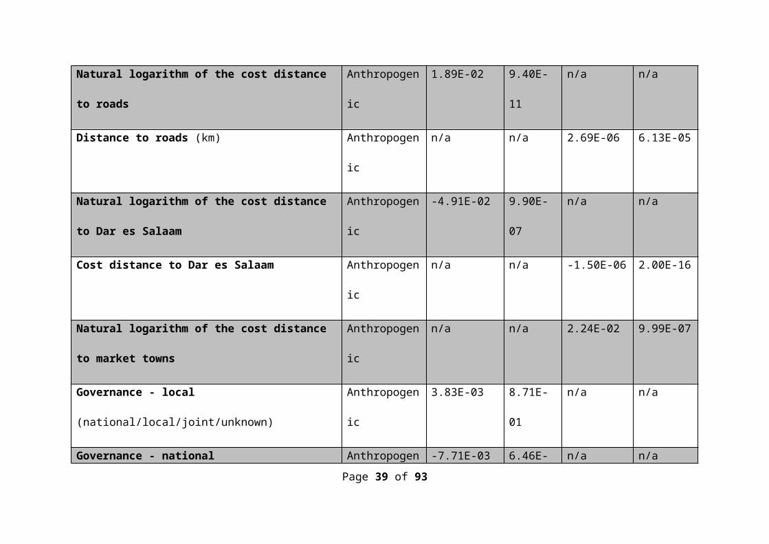
Table S1 The coefficients and associated p-values of the variables correlated with WSG using both forward and backward selection procedures.

Variable (where appropriate, units are given in brackets) Group Forward Backward

Coefficient p-value Coefficient p-value

(Intercept) n/a -1.98E+02 2.14E-05 -1.59E+02 6.20E-04

Natural logarithm of the population pressure with

decay constant of 16.7km

Anthropogenic -7.33E-03 9.78E-02 n/a n/a



Anthropogenic n/a n/a -1.33E-02 5.20E-03

Natural logarithm of the cost distance to roads Anthropogenic 1.89E-02 9.40E-11 n/a n/a

Distance to roads (km) Anthropogenic n/a n/a 2.69E-06 6.13E-05

Natural logarithm of the cost distance to Dar es Salaam Anthropogenic -4.91E-02 9.90E-07 n/a n/a

Cost distance to Dar es Salaam Anthropogenic n/a n/a -1.50E-06 2.00E-16

of 61

498

499

Natural logarithm of the cost distance to market towns Anthropogenic n/a n/a 2.24E-02 9.99E-07

Governance - local (national/local/joint/unknown) Anthropogenic 3.83E-03 8.71E-01 n/a n/a

Governance - national (national/local/joint/unknown) Anthropogenic -7.71E-03 6.46E-02 n/a n/a

Governance - unknown (national/local/joint/unknown) Anthropogenic 3.93E-02 1.17E-01 n/a n/a

Mean annual monthly temperature range (°C) Climatic 2.90E-02 2.00E-16 n/a n/a

Mean annual maximum monthly temperature (°C) Climatic n/a n/a 2.62E-02 2.00E-16

Mean annual minimum monthly temperature (°C) Climatic n/a n/a -2.53E-02 2.00E-16

Wind speed (m s-1) Climatic -3.70E-05 2.04E-02 -4.98E-05 7.84E-04

Mean number of dry months annually Climatic n/a n/a 3.71E-03 2.51E-02

pH of the soil Edaphic 9.68E-02 2.00E-16 8.63E-02 1.27E-12

Total available water capacity of the soil (vol. %, -33 to

-1500kPA conforming to USDA standards)

Edaphic -1.22E-02 3.90E-09 -7.01E-03 4.59E-02

Total nitrogen content of the soil (g kg-1) Edaphic n/a n/a 7.14E-03 1.31E-02

of 61

Total carbon content of the soil (g kg-1) Edaphic n/a n/a 5.59E-02 8.35E-02

Percentage sand content of the soil (%) Edaphic n/a n/a 3.99E-03 2.02E-03

Annual mean burned area probability Fire 2.63E+01 3.80E-06 2.09E+01 2.62E-04

Mean annual global horizontal solar radiation (kW m-2

day-1)

Geographic 7.47E-05 3.40E-04 7.93E-05 1.32E-04

Spatial autocorrelation term 4 Spatial -4.88E+00 3.20E-04 -1.16E+01 1.28E-03

Spatial autocorrelation term 6 Spatial 1.04E-01 5.83E-08 8.83E-02 2.92E-06

Spatial autocorrelation term 8 Spatial 1.27E-01 1.34E-04 n/a n/a

Spatial autocorrelation term 5 Spatial 9.83E+00 1.61E-05 n/a n/a

Spatial autocorrelation term 2 Spatial -1.18E-01 1.46E-05 7.70E+00 5.15E-04

Spatial autocorrelation term 1 Spatial n/a n/a -7.79E+00 5.14E-04

Spatial autocorrelation term 3 Spatial n/a n/a 7.89E+00 5.27E-04

of 61

500

Table S2 The coefficients and associated p-values of the variables correlated with the intercept of the power law relationship using both forward

and backward selection procedures.

Variable (where appropriate, units are given in

brackets)

Group Forward Backward


(Intercept) n/a -2.95E+01 1.89E-11 -5.37E+02 9.92E-08

Natural logarithm of the cost distance to roads Anthropogenic -5.29E-01 9.09E-10 -3.09E-01 1.05E-04

Historical logging – Partially logged (no

logging/partially logged) Anthropogenic 1.06E+00 1.68E-05 1.67E+00 2.18E-09


decay constant of 12.5km Anthropogenic 8.45E-01 1.23E-12 4.98E-01 1.06E-05

Cost distance to Dar es Salaam Anthropogenic 1.40E-05 3.47E-06 n/a n/a

Mean annual monthly temperature range (°C) Climatic 8.46E-01 2.00E-16 9.52E-01 2.00E-16

Total available water capacity of the soil (g kg-1) Edaphic 2.72E-01 3.82E-10 2.47E-01 1.22E-07

of 61

501

502

Mean burned area probability in the fourth quarter Fire n/a n/a 2.05E+02 1.27E-03

Mean annual global horizontal solar radiation (kW

m-2 day-1) Geographic 3.64E-03 9.90E-08 3.76E-03 4.37E-07





of 61

503

Table S3 The coefficients and associated p-values of the variables correlated with the gradient of the power law relationship using both forward

and backward selection procedures.

Variable (where appropriate, units are given in brackets) Group Forward Backward


(Intercept) n/a 7.74E+00 1.05E-10 9.21E+01 1.53E-04

Natural logarithm of the cost distance to roads Anthropogenic 1.22E-01 1.12E-08 6.05E-02 1.15E-03

Historical logging (no logging/partially logged) Anthropogenic -1.01E-01 9.71E-02 -2.95E-01 8.78E-06

Natural logarithm of the population pressure with decay

constant of 20.8km Anthropogenic -2.50E-01 6.99E-10 -1.75E-01 2.91E-05

Cost distance to Dar es Salaam Anthropogenic -3.76E-06 1.62E-06 n/a n/a

Mean annual monthly temperature range (°C) Climatic -2.05E-01 2.00E-16 -2.38E-01 2.00E-16

Total available water capacity of the soil (g kg-1) Edaphic -5.40E-02 1.24E-07 -4.16E-02 2.10E-04

Mean burned area probability in the fourth quarter Fire -5.81E+01 1.23E-04 -5.62E+01 2.51E-04

of 61

504

505

Mean annual global horizontal solar radiation (kW m-2 day-1) Geographic -8.68E-04 4.20E-07 -1.05E-03 2.47E-08




Spatial autocorrelation term 6 Spatial n/a n/a -2.08E-01 9.66E-04

of 61

506

Table S4 The PC axes derived from the candidate variables (Table S6). Axes shown in this study to significantly affect carbon sequestration are

indicated by an asterisk.

Variable PC1

Coefficient*

PC2

Coefficient

PC3

Coefficient*

PC4

Coefficient

PC5

Coefficient*

Population pressure with decay constant of 41.6km 0.18 -0.08 -0.03 -0.12 0

Population pressure with decay constant of 20.8km 0.19 -0.02 0.02 -0.04 0.01

Population pressure with decay constant of 16.7km 0.19 -0.02 0.02 -0.02 0.01

Population pressure with decay constant of 12.5km 0.19 -0.01 0.02 -0.01 -0.01

Population pressure with decay constant of 8.6km 0.19 -0.02 0 -0.01 -0.05

Population pressure with decay constant of 4.2km 0.18 -0.06 -0.03 -0.05 -0.09

Population pressure with decay constant of 1.7km 0.17 -0.08 -0.07 -0.08 -0.07


constant of 41.6km

0.18 -0.06 -0.01 -0.16 -0.03


constant of 20.8km

0.18 0.08 0.08 -0.04 -0.02

of 61

507

508


constant of 16.7km

0.18 0.09 0.09 -0.02 -0.03


constant of 12.5km

0.18 0.11 0.09 -0.01 -0.05


constant of 8.6km

0.18 0.1 0.07 0 -0.08


constant of 4.2km

0.18 0.05 -0.02 0.01 -0.17


constant of 1.7km

0.12 -0.04 -0.22 -0.05 -0.26

Cost distance to Dar es Salaam -0.17 0.01 0.22 -0.08 -0.01

Cost distance to market towns -0.12 -0.14 0.3 0.06 0.04

Distance to roads -0.1 -0.22 0.09 -0.08 -0.24

Distance to Dar es Salaam -0.16 0.04 -0.03 -0.32 -0.1

Distance to market towns -0.13 -0.21 -0.09 0.02 0

Natural logarithm of the cost distance to Dar es Salaam -0.17 0.02 0.19 -0.05 -0.03

of 61

Natural logarithm of the cost distance to market towns -0.11 -0.15 0.3 0.08 -0.02

Natural logarithm of the cost distance to roads -0.09 -0.23 0.15 -0.04 -0.22

Mean annual temperature -0.08 0.17 -0.32 0.1 -0.17

Mean annual maximum monthly temperature -0.1 0.14 -0.3 0.06 -0.15

Mean annual minimum monthly temperature -0.06 0.19 -0.31 0.12 -0.18

Mean annual monthly temperature range -0.07 -0.22 0.14 -0.19 0.19

Mean maximum cumulative water deficit -0.1 -0.15 -0.21 -0.14 0.06

Mean number of dry months annually -0.03 -0.25 -0.18 -0.05 0.03

Wind speed 0.16 -0.14 -0.04 0.12 0.11

Total nitrogen content of the soil -0.02 -0.17 -0.03 -0.11 -0.53

Total carbon content of the soil 0.01 -0.23 0.15 0.31 -0.13

Percentage sand content of the soil -0.06 0.17 -0.12 -0.23 0.43

Total available water capacity of the soil 0.01 0.18 0.21 0.41 0.03

pH of the soil 0 0.23 0.17 0.28 -0.19

Soil fertility 0 -0.29 -0.04 -0.05 0.02

Mean burned area probability in the fourth quarter -0.12 -0.2 -0.15 0.17 0.07

of 61

Mean burned area probability in the third quarter -0.12 -0.2 -0.15 0.17 0.07

Annual mean burned area probability -0.12 -0.2 -0.15 0.17 0.07

Aspect 0.03 0.14 0.06 -0.24 0.1

Mean annual global horizontal solar radiation -0.11 0 -0.17 0.31 0.17

Spatial autocorrelation term 1 0.18 -0.08 -0.03 0.08 0.08





Spatial autocorrelation term 6 -0.17 0.14 0.04 -0.07 -0.07



of 61

509

510

Table S5 The coefficients and associated p-values of the correlations between the derivatives of carbon storage (the intercept of the power law

relationship, the gradient of the power law relationship, WSG and maximum canopy height [shown here are intercept, gradient, WSG and height

respectively]) and the carbon storage estimates made in this study.

Variable 4th order interactions 2nd order interactions


(Intercept) 2.77E+03 2.00E-16 5.08E+02 2.00E-16

height -8.61E+01 2.00E-16 -2.71E+00 3.99E-07

intercept 2.79E+02 2.00E-16 1.93E+02 2.00E-16

gradient 3.97E+03 2.00E-16 1.04E+03 2.00E-16

WSG -4.25E+03 2.00E-16 -5.95E+02 2.00E-16

height:intercept -9.12E+00 5.61E-12 -2.10E+00 2.00E-16

height:gradient -1.32E+02 2.00E-16 -7.53E+00 2.00E-16

height:WSG 1.42E+02 2.00E-16 8.23E+00 2.00E-16

intercept:gradient -1.64E+02 2.00E-16 -4.33E+00 2.00E-16

of 61

511

512

513

intercept:WSG -3.59E+02 6.84E-12 -2.27E+02 2.00E-16

gradient:WSG -5.87E+03 2.00E-16 -1.20E+03 2.00E-16

height:intercept:gradient 5.90E+00 2.00E-16 n/a n/a

height:intercept:WSG 1.09E+01 5.36E-07 n/a n/a

height:gradient:WSG 1.98E+02 2.00E-16 n/a n/a

intercept:gradient:WSG 2.55E+02 2.00E-16 n/a n/a

height:intercept:gradient:WSG -9.38E+00 2.00E-16 n/a n/a

of 61

514

515

Table S6 The candidate drivers used in this investigation divided into six groups (anthropogenic, climatic, edaphic, fire, geographic, and spatial). The possible effects of these drivers on forest carbon storage and sequestration, wood specific gravity and population structure has been provided.

Candidate Driver Name Candidate Driver Description Resolution Data Source

Group

Carbon Storage and Sequestration (References)

Wood Specific Gravity

(References)

Population Structure(References)

Population pressure with decay constant of 41.6km

The population pressure experienced by an area, derived using a 41.6km decay constant

0.1km Raw pop data [100] post-

processed as described in

[99]

Anthropogenic

Logging and other forms of disturbance

reduce the carbon stored in tropical forest. Increased

disturbance will also result in increased carbon emissions.

[107-110]


will result in a decrease of shade

tolerant trees and a consequent increase in

light demanding species. This will be

associated with a reduction in WSG.

[111]


will result in a decrease of shade

tolerant trees and a consequent increase in

light demanding species. Larger trees will be preferentially

removed, leaving forests dominated by many small stems.

[97, 110, 111]










The population pressure experienced by an area, derived using a 4.1.7km decay constant



Natural logarithm of the population pressure with decay constant of

41.6km

Log transformation of the population pressure experienced by an area, derived using a 41.6km decay

constant. Unit addition avoids Logn(0)Natural logarithm of the population

pressure with decay constant of 20.8km













Log transformation of the population pressure experienced by an area, derived using a 4.1.7km

decay constant. Unit addition avoids Logn(0)Natural logarithm of the population



constant. Unit addition avoids Logn(0)

of 61

516517518

Cost distance to Dar es Salaam The cost distance to Dar es Salaam according to road type (A, B or C), protected areas and water bodies

0.1km N/A

Cost distance to market towns The cost distance to market towns according to road type (A, B or C), protected areas and water bodies

Distance to roads The euclidean distance to nearest A or B roadDistance to Dar es Salaam The euclidean distance to Dar es Salaam

Distance to market townsThe euclidean distance to nearest market town

(defined as a settlement with a population ≥ 5000 in 2002 census)

Natural logarithm of the cost distance to Dar es Salaam

Log transformation of the cost distance to Dar es Salaam. Unit addition avoids Logn(0)

Natural logarithm of the cost distance to market towns

Log transformation of the cost distance to a market town. Unit addition avoids Logn(0)

Natural logarithm of the cost distance to roads

Log transformation of the cost distance to nearest A or B road. Unit addition avoids Logn(0)

Historical logging

An attempt to record for each forest reserve an indication of the past logging history. Areas were

assigned one of four categories: no logging, partially logged, clear felled and no data

0.1km [112]

GovernanceThe governance of the land. Land categories were

divided into those under national control, local control, joint management and unknown.

Various [113]

Mean annual temperature

The mean annual temperature derived from the mean monthly temperatures. Made more resolute using the

elevation difference observed between the climate data digital elevation model and a higher resolution

dataset

0.1km [29, 114]Climatic

Temperatures increases and extreme droughts will decrease

forest productivity, and therefore carbon

storage and sequestration.

However, carbon storage may increase with increased levels of gradual drought.

[53, 62, 72, 107, 115]

WSG will increase with increased levels

of drought. Other climatic factors may also be important.

[62, 72, 89]

Changes in climate will alter species

composition. Increasing amounts of precipitation and an

increasing temperature range will result in

increasing stem density.

[62, 97, 98, 116]

Mean annual maximum monthly temperature

The mean annual maximum temperature derived from the mean monthly maximum temperatures. Made

more resolute using the elevation difference observed between the climate data digital elevation model and

a higher resolution dataset

Mean annual minimum monthly temperature

The mean annual minimum temperature derived from the mean monthly minimum temperatures. Made

more resolute using the elevation difference observed between the climate data digital elevation model and

a higher resolution datasetMean annual monthly temperature

rangeThe difference between the mean annual maximum

and minimum temperaturesMean maximum cumulative water

deficitMaximum mean cumulative water deficit (calculated

as [53])4km [117, 118]

Mean number of dry months annuallyThe average number of months annually that

precipitation is exceeded by potential evapotranspiration

Wind speed The mean annual wind speed 50m above the ground 0.2km [119]

of 61

Total nitrogen content of the soil The amount of organic carbon present in the soil to a depth of 1m

10km [103, 104]

Edaphic

More fertile areas will show greater growth rates and increased

levels of carbon storage.

[62, 107]

More fertile areas will show lower WSG

values.[62]

As soil fertility increases, stem density

will increase. There will also be more large

stems.[62, 97, 98]

Total carbon content of the soil The amount of nitrogen present in the soil to a depth of 1m

Percentage sand content of the soil The mean percentage mass of sand in the soil to a depth of 1m

Total available water capacity of the soil

The available water capacity of the soil to a depth of 1m

pH of the soil The mean pH of the soil to a depth of 1m

Soil fertilityA mean measure of soil fertility to a 1m depth.

Calculated as ((100-Aluminium saturation)/100)*effective cation exchange capacity

Mean burned area probability in the fourth quarter

The mean burnt area probability from January to March

0.5km [120]

Fire

Areas that experience burns more frequently

will show lower carbon storage levels.

Overall, they will show lower rates of growth, but during

recovery from a burn, growth rates may be

increased.[121, 122]

Areas that experience burns more frequently will show lower WSG

values.[121]

An increased probability of fire will result in a decreasing

stem density.[121-123]

Mean burned area probability in the third quarter The mean burnt area probability from April to June

Mean burned area probability in the second quarter

The mean burnt area probability from July to September

Mean burned area probability in the first quarter

The mean burnt area probability from October to December

Annual mean burned area probability The annual mean burned area probability

Aspect The aspect of the slope 0.1km [114] Geographic

Higher solar radiation results in high levels of growth and carbon

storage.[98, 124]

Light demanding pioneers show lower

wood density.[111]

Higher solar radiation levels may lead to

increased tree densities and also an increased proportion of larger

stems.[97, 98]

Mean annual global horizontal solar radiation

The mean annual global horizontal solar radiation at ground level 40km [125, 126]

Spatial autocorrelation term 1 Latitude + Longitude + Latitude*Latitude + Longitude*Longitude + Longitude*Latitude

0.1km N/A

Spatial

None - included in the model to help account

for landscape scale spatial autocorrelation.

[127-129]



[127-129]



[127-129]

Spatial autocorrelation term 2 Latitude + Longitude + Latitude*Latitude + Longitude*Longitude

Spatial autocorrelation term 3 Latitude + Longitude + Longitude*LatitudeSpatial autocorrelation term 4 LatitudeSpatial autocorrelation term 5 LongitudeSpatial autocorrelation term 6 Latitude*LatitudeSpatial autocorrelation term 7 Longitude*LongitudeSpatial autocorrelation term 8 Longitude*Latitude

of 61

519

of 61

520

Table S7 The correlation coefficients of the continuous candidate drivers.

ID Candidate Driver Name 1 2 3 4 5 6 7 8 9 10 11 12 13 14 15 16 17 18 19 20 21 22 23 24 25 26 27 28 29 30 31 32 33 34 35 36 37 38 39 40 41 42 43 44 45 46 47 48 49 50

1

Population pressure with


1.0 0.9 0.8 0.7 0.5 0.5 0.4 1.0 0.9 0.8 0.8 0.7 0.7 0.6 -0.8

-0.5

-0.4

-0.8

-0.5

-0.8

-0.5

-0.3

-0.1 0.0 -

0.2 0.5 -0.4 0.0 0.9 -

0.3-

0.6 0.1 -0.3

-0.4 0.0 -

0.1-

0.1 NA NA -0.1

-0.1

-0.5 0.9 0.9 0.9 0.9 0.9 -

0.9 0.9 0.9

2



0.9 1.0 1.0 0.9 0.8 0.7 0.6 0.9 1.0 0.9 0.9 0.9 0.8 0.7 -0.8

-0.5

-0.5

-0.9

-0.7

-0.8

-0.5

-0.3

-0.2

-0.1

-0.2 0.4 -

0.5-

0.2 0.7 -0.2

-0.4

-0.1

-0.2

-0.2

-0.1

-0.1

-0.1 NA NA -

0.1-

0.1-

0.6 0.8 0.8 0.7 0.8 0.8 -0.8 0.8 0.7

3



0.8 1.0 1.0 1.0 0.9 0.8 0.6 0.8 0.9 0.9 0.9 0.9 0.8 0.7 -0.7

-0.5

-0.5

-0.9

-0.7

-0.7

-0.5

-0.3

-0.2

-0.1

-0.2 0.3 -

0.6-

0.2 0.6 -0.2

-0.3

-0.1

-0.2

-0.1

-0.1

-0.1

-0.1 NA NA -

0.1-

0.1-

0.6 0.7 0.7 0.6 0.6 0.7 -0.7 0.7 0.6

4



0.7 0.9 1.0 1.0 1.0 0.9 0.6 0.7 0.8 0.9 0.9 0.9 0.8 0.7 -0.6

-0.5

-0.5

-0.8

-0.6

-0.7

-0.5

-0.3

-0.2

-0.2

-0.2 0.3 -

0.6-

0.3 0.5 -0.1

-0.2

-0.1

-0.1 0.0 -

0.2-

0.1-

0.1 NA NA -0.1

-0.1

-0.6 0.6 0.6 0.5 0.5 0.6 -

0.5 0.6 0.5

5



0.5 0.8 0.9 1.0 1.0 0.9 0.7 0.6 0.7 0.8 0.8 0.8 0.7 0.6 -0.6

-0.4

-0.4

-0.7

-0.5

-0.6

-0.4

-0.3

-0.2

-0.2

-0.2 0.3 -

0.5-

0.3 0.4 -0.1

-0.1

-0.2

-0.1 0.0 -

0.2-

0.1-

0.1 NA NA -0.1

-0.1

-0.5 0.4 0.5 0.4 0.4 0.5 -

0.4 0.5 0.4

6



0.5 0.7 0.8 0.9 0.9 1.0 0.8 0.5 0.7 0.7 0.7 0.7 0.7 0.6 -0.5

-0.4

-0.4

-0.6

-0.5

-0.5

-0.4

-0.3

-0.2

-0.2

-0.2 0.2 -

0.4-

0.3 0.4 -0.1 0.0 -

0.1-

0.1 0.1 -0.2

-0.1

-0.1 NA NA -

0.1-

0.1-

0.4 0.4 0.4 0.3 0.3 0.4 -0.4 0.4 0.3

7



0.4 0.6 0.6 0.6 0.7 0.8 1.0 0.4 0.5 0.6 0.6 0.6 0.6 0.6 -0.5

-0.4

-0.4

-0.5

-0.4

-0.5

-0.5

-0.4

-0.1 0.0 -

0.1 0.2 -0.2

-0.1 0.3 -

0.2-

0.1-

0.1-

0.2 0.1 -0.2 0.0 0.0 NA NA 0.0 0.0 -

0.3 0.4 0.4 0.3 0.3 0.4 -0.4 0.4 0.3

8

Natural logarithm of the

population pressure with


1.0 0.9 0.8 0.7 0.6 0.5 0.4 1.0 0.9 0.8 0.8 0.7 0.7 0.6 -0.8

-0.5

-0.4

-0.8

-0.5

-0.8

-0.5

-0.3

-0.2 0.0 -

0.2 0.5 -0.4 0.0 0.9 -

0.3-

0.6 0.1 -0.3

-0.4 0.0 -

0.1-

0.1 NA NA -0.1

-0.1

-0.5 0.9 0.9 0.9 0.9 0.9 -

0.9 0.9 0.9

9




0.9 1.0 0.9 0.8 0.7 0.7 0.5 0.9 1.0 1.0 1.0 0.9 0.8 0.7 -0.8

-0.6

-0.6

-0.9

-0.7

-0.8

-0.6

-0.4

-0.1 0.0 -

0.1 0.3 -0.5

-0.1 0.8 -

0.3-

0.4-

0.1-

0.1-

0.1-

0.3-

0.1-

0.2 NA NA -0.2

-0.1

-0.5 0.8 0.9 0.8 0.8 0.8 -

0.8 0.8 0.8

of 61

521

10




0.8 0.9 0.9 0.9 0.8 0.7 0.6 0.8 1.0 1.0 1.0 1.0 0.8 0.7 -0.8

-0.6

-0.6

-0.9

-0.8

-0.8

-0.6

-0.4 0.0 0.0 -

0.1 0.2 -0.5

-0.1 0.7 -

0.3-

0.3-

0.1-

0.1 0.0 -0.3

-0.1

-0.2 NA NA -

0.2-

0.1-

0.5 0.8 0.8 0.7 0.7 0.8 -0.7 0.8 0.7

11




0.8 0.9 0.9 0.9 0.8 0.7 0.6 0.8 1.0 1.0 1.0 1.0 0.9 0.7 -0.8

-0.7

-0.6

-0.8

-0.8

-0.8

-0.7

-0.4 0.0 0.0 -

0.1 0.2 -0.5

-0.1 0.7 -

0.4-

0.2-

0.1-

0.1 0.1 -0.4

-0.1

-0.1 NA NA -

0.1-

0.1-

0.5 0.7 0.8 0.6 0.7 0.8 -0.7 0.8 0.6

12




0.7 0.9 0.9 0.9 0.8 0.7 0.6 0.7 0.9 1.0 1.0 1.0 1.0 0.9 -0.9

-0.7

-0.7

-0.8

-0.7

-0.8

-0.7

-0.5

-0.1 0.0 -

0.1 0.2 -0.4

-0.1 0.6 -

0.4-

0.2-

0.1-

0.1 0.2 -0.5

-0.1

-0.1 NA NA -

0.1-

0.1-

0.4 0.7 0.8 0.6 0.7 0.7 -0.7 0.7 0.6

13




0.7 0.8 0.8 0.8 0.7 0.7 0.6 0.7 0.8 0.8 0.9 1.0 1.0 1.0 -0.9

-0.7

-0.6

-0.8

-0.6

-0.8

-0.7

-0.5

-0.2

-0.1

-0.2 0.3 -

0.4-

0.2 0.7 -0.5

-0.2

-0.1

-0.1 0.2 -

0.5 0.0 0.0 NA NA 0.0 -0.2

-0.3 0.7 0.7 0.7 0.7 0.7 -

0.7 0.7 0.7

14




0.6 0.7 0.7 0.7 0.6 0.6 0.6 0.6 0.7 0.7 0.7 0.9 1.0 1.0 -0.9

-0.7

-0.5

-0.7

-0.5

-0.8

-0.7

-0.5

-0.2

-0.1

-0.3 0.4 -

0.3-

0.1 0.6 -0.5

-0.1

-0.1

-0.1 0.2 -

0.5 0.0 0.0 NA NA 0.0 -0.2

-0.2 0.7 0.7 0.6 0.7 0.7 -

0.7 0.7 0.6

15 Cost distance to Dar es Salaam

-0.8

-0.8

-0.7

-0.6

-0.6

-0.5

-0.5

-0.8

-0.8

-0.8

-0.8

-0.9

-0.9

-0.9 1.0 0.9 0.8 0.8 0.7 1.0 0.9 0.6 -

0.1-

0.1 0.0 -0.3 0.3 0.0 -

0.7 0.5 0.3 0.0 0.2 0.0 0.4 0.0 0.0 NA NA 0.0 0.1 0.3 -0.8

-0.8

-0.8

-0.8

-0.8 0.8 -

0.8-

0.8

16 Cost distance to market towns

-0.5

-0.5

-0.5

-0.5

-0.4

-0.4

-0.4

-0.5

-0.6

-0.6

-0.7

-0.7

-0.7

-0.7 0.9 1.0 0.8 0.5 0.7 0.8 0.9 0.6 -

0.3-

0.3-

0.3 0.1 0.1 -0.2

-0.4 0.5 0.1 0.1 0.1 -

0.2 0.5 0.0 0.0 NA NA 0.0 0.0 0.2 -0.5

-0.6

-0.5

-0.5

-0.5 0.5 -

0.5-

0.5

17 Distance to roads

-0.4

-0.5

-0.5

-0.5

-0.4

-0.4

-0.4

-0.4

-0.6

-0.6

-0.6

-0.7

-0.6

-0.5 0.8 0.8 1.0 0.4 0.6 0.7 0.7 0.9 -

0.1-

0.1-

0.1 0.0 0.2 0.0 -0.3 0.3 0.3 -

0.1 0.1 -0.1 0.4 0.0 0.0 NA NA 0.0 0.1 0.2 -

0.4-

0.5-

0.4-

0.4-

0.4 0.4 -0.4

-0.4

18 Distance to Dar es Salaam

-0.8

-0.9

-0.9

-0.8

-0.7

-0.6

-0.5

-0.8

-0.9

-0.9

-0.8

-0.8

-0.8

-0.7 0.8 0.5 0.4 1.0 0.5 0.8 0.5 0.3 0.2 0.1 0.3 -

0.5 0.5 0.2 -0.8 0.3 0.4 0.0 0.2 0.1 0.2 0.1 0.1 NA NA 0.1 0.1 0.5 -

0.9-

0.9-

0.8-

0.8-

0.9 0.9 -0.9

-0.8

19 Distance to market towns

-0.5

-0.7

-0.7

-0.6

-0.5

-0.5

-0.4

-0.5

-0.7

-0.8

-0.8

-0.7

-0.6

-0.5 0.7 0.7 0.6 0.5 1.0 0.6 0.7 0.3 -

0.3-

0.3-

0.3 0.2 0.3 -0.1

-0.4 0.4 0.1 0.2 -

0.1-

0.2 0.4 0.1 0.2 NA NA 0.2 0.0 0.5 -0.5

-0.5

-0.4

-0.4

-0.5 0.4 -

0.5-

0.4

20

Natural logarithm of the cost distance to Dar es Salaam

-0.8

-0.8

-0.7

-0.7

-0.6

-0.5

-0.5

-0.8

-0.8

-0.8

-0.8

-0.8

-0.8

-0.8 1.0 0.8 0.7 0.8 0.6 1.0 0.8 0.6 0.0 -

0.1 0.0 -0.3 0.3 0.0 -

0.8 0.5 0.4 -0.1 0.2 0.1 0.4 0.0 0.1 NA NA 0.1 0.1 0.3 -

0.9-

0.9-

0.8-

0.9-

0.9 0.9 -0.9

-0.8

of 61

21

Natural logarithm of the cost distance to market towns

-0.5

-0.5

-0.5

-0.5

-0.4

-0.4

-0.5

-0.5

-0.6

-0.6

-0.7

-0.7

-0.7

-0.7 0.9 0.9 0.7 0.5 0.7 0.8 1.0 0.7 -

0.3-

0.3-

0.3 0.1 0.1 -0.2

-0.4 0.6 0.1 0.1 0.1 -

0.3 0.6 0.0 0.1 NA NA 0.1 0.0 0.1 -0.5

-0.6

-0.5

-0.5

-0.6 0.5 -

0.6-

0.5

22

Natural logarithm of the cost distance to

roads

-0.3

-0.3

-0.3

-0.3

-0.3

-0.3

-0.4

-0.3

-0.4

-0.4

-0.4

-0.5

-0.5

-0.5 0.6 0.6 0.9 0.3 0.3 0.6 0.7 1.0 0.0 0.0 0.1 -

0.1 0.2 0.1 -0.3 0.3 0.3 -

0.2 0.1 -0.1 0.3 0.0 0.0 NA NA 0.0 0.1 0.1 -

0.4-

0.4-

0.3-

0.4-

0.4 0.3 -0.4

-0.3

23 Mean annual temperature

-0.1

-0.2

-0.2

-0.2

-0.2

-0.2

-0.1

-0.2

-0.1 0.0 0.0 -

0.1-

0.2-

0.2-

0.1-

0.3-

0.1 0.2 -0.3 0.0 -

0.3 0.0 1.0 1.0 1.0 -0.6 0.3 0.4 -

0.1-

0.4 0.1 0.0 0.0 0.2 -0.3

-0.1

-0.1 NA NA -

0.1 0.2 0.1 -0.1 0.0 -

0.2-

0.1-

0.1 0.2 -0.1

-0.2

24

Mean annual maximum monthly

temperature

0.0 -0.1

-0.1

-0.2

-0.2

-0.2 0.0 0.0 0.0 0.0 0.0 0.0 -

0.1-

0.1-

0.1-

0.3-

0.1 0.1 -0.3

-0.1

-0.3 0.0 1.0 1.0 0.9 -

0.4 0.4 0.4 0.0 -0.4 0.0 0.1 0.0 0.1 -

0.2 0.0 -0.1 NA NA -

0.1 0.2 0.1 0.0 0.1 0.0 0.0 0.1 0.0 0.1 0.0

25

Mean annual minimum monthly

temperature

-0.2

-0.2

-0.2

-0.2

-0.2

-0.2

-0.1

-0.2

-0.1

-0.1

-0.1

-0.1

-0.2

-0.3 0.0 -

0.3-

0.1 0.3 -0.3 0.0 -

0.3 0.1 1.0 0.9 1.0 -0.7 0.3 0.4 -

0.2-

0.3 0.2 -0.1 0.1 0.3 -

0.3-

0.1-

0.1 NA NA -0.1 0.2 0.1 -

0.2-

0.1-

0.2-

0.2-

0.1 0.3 -0.1

-0.2

26

Mean annual monthly

temperature range

0.5 0.4 0.3 0.3 0.3 0.2 0.2 0.5 0.3 0.2 0.2 0.2 0.3 0.4 -0.3 0.1 0.0 -

0.5 0.2 -0.3 0.1 -

0.1-

0.6-

0.4-

0.7 1.0 -0.1

-0.3 0.5 0.1 -

0.5 0.3 -0.2

-0.4 0.2 0.1 0.1 NA NA 0.1 -

0.2-

0.2 0.5 0.4 0.5 0.5 0.4 -0.6 0.4 0.5

27

Mean maximum cumulative

water deficit

-0.4

-0.5

-0.6

-0.6

-0.5

-0.4

-0.2

-0.4

-0.5

-0.5

-0.5

-0.4

-0.4

-0.3 0.3 0.1 0.2 0.5 0.3 0.3 0.1 0.2 0.3 0.4 0.3 -

0.1 1.0 0.6 -0.3 0.1 0.3 -

0.1-

0.1 0.1 0.0 0.1 0.1 NA NA 0.1 0.1 0.4 -0.3

-0.4

-0.3

-0.3

-0.3 0.3 -

0.3-

0.3

28Mean number of dry months

annually0.0 -

0.2-

0.2-

0.3-

0.3-

0.3-

0.1 0.0 -0.1

-0.1

-0.1

-0.1

-0.2

-0.1 0.0 -

0.2 0.0 0.2 -0.1 0.0 -

0.2 0.1 0.4 0.4 0.4 -0.3 0.6 1.0 0.1 -

0.1 0.1 -0.2

-0.2 0.0 0.0 0.1 0.1 NA NA 0.1 0.1 0.2 0.1 0.1 0.1 0.1 0.1 -

0.1 0.1 0.1

29 Wind speed 0.9 0.7 0.6 0.5 0.4 0.4 0.3 0.9 0.8 0.7 0.7 0.6 0.7 0.6 -0.7

-0.4

-0.3

-0.8

-0.4

-0.8

-0.4

-0.3

-0.1 0.0 -

0.2 0.5 -0.3 0.1 1.0 -

0.4-

0.6 0.1 -0.3

-0.3

-0.1

-0.1

-0.1 NA NA -

0.1-

0.1-

0.3 1.0 1.0 1.0 1.0 1.0 -1.0 1.0 1.0

30Total nitrogen content of the

soil

-0.3

-0.2

-0.2

-0.1

-0.1

-0.1

-0.2

-0.3

-0.3

-0.3

-0.4

-0.4

-0.5

-0.5 0.5 0.5 0.3 0.3 0.4 0.5 0.6 0.3 -

0.4-

0.4-

0.3 0.1 0.1 -0.1

-0.4 1.0 0.2 -

0.4-

0.1-

0.4 0.8 0.1 0.1 NA NA 0.1 0.1 -0.2

-0.4

-0.4

-0.4

-0.4

-0.4 0.4 -

0.4-

0.4

31Total carbon content of the

soil

-0.6

-0.4

-0.3

-0.2

-0.1 0.0 -

0.1-

0.6-

0.4-

0.3-

0.2-

0.2-

0.2-

0.1 0.3 0.1 0.3 0.4 0.1 0.4 0.1 0.3 0.1 0.0 0.2 -0.5 0.3 0.1 -

0.6 0.2 1.0 -0.7 0.1 0.5 -

0.1 0.0 0.0 NA NA 0.0 0.1 0.2 -0.6

-0.6

-0.6

-0.6

-0.6 0.6 -

0.6-

0.6

32Percentage sand content of the

soil0.1 -

0.1-

0.1-

0.1-

0.2-

0.1-

0.1 0.1 -0.1

-0.1

-0.1

-0.1

-0.1

-0.1 0.0 0.1 -

0.1 0.0 0.2 -0.1 0.1 -

0.2 0.0 0.1 -0.1 0.3 -

0.1-

0.2 0.1 -0.4

-0.7 1.0 0.0 -

0.3-

0.1 0.1 0.0 NA NA 0.0 -0.1 0.1 0.1 0.1 0.2 0.1 0.1 -

0.1 0.1 0.2

33Total available water capacity

of the soil

-0.3

-0.2

-0.2

-0.1

-0.1

-0.1

-0.2

-0.3

-0.1

-0.1

-0.1

-0.1

-0.1

-0.1 0.2 0.1 0.1 0.2 -

0.1 0.2 0.1 0.1 0.0 0.0 0.1 -0.2

-0.1

-0.2

-0.3

-0.1 0.1 0.0 1.0 0.7 -

0.4 0.0 0.0 NA NA 0.0 0.0 0.1 -0.3

-0.3

-0.3

-0.3

-0.3 0.3 -

0.3-

0.3

34 pH of the soil -0.4

-0.2

-0.1 0.0 0.0 0.1 0.1 -

0.4-

0.1 0.0 0.1 0.2 0.2 0.2 0.0 -0.2

-0.1 0.1 -

0.2 0.1 -0.3

-0.1 0.2 0.1 0.3 -

0.4 0.1 0.0 -0.3

-0.4 0.5 -

0.3 0.7 1.0 -0.8 0.0 0.0 NA NA 0.0 0.0 0.2 -

0.3-

0.2-

0.3-

0.3-

0.2 0.3 -0.2

-0.3

of 61

35 Soil fertility 0.0 -0.1

-0.1

-0.2

-0.2

-0.2

-0.2 0.0 -

0.3-

0.3-

0.4-

0.5-

0.5-

0.5 0.4 0.5 0.4 0.2 0.4 0.4 0.6 0.3 -0.3

-0.2

-0.3 0.2 0.0 0.0 -

0.1 0.8 -0.1

-0.1

-0.4

-0.8 1.0 0.0 0.1 NA NA 0.1 0.1 -

0.2-

0.2-

0.2-

0.1-

0.1-

0.2 0.1 -0.2

-0.1

36

Mean burned area probability

in the fourth quarter

-0.1

-0.1

-0.1

-0.1

-0.1

-0.1 0.0 -

0.1-

0.1-

0.1-

0.1-

0.1 0.0 0.0 0.0 0.0 0.0 0.1 0.1 0.0 0.0 0.0 -0.1 0.0 -

0.1 0.1 0.1 0.1 -0.1 0.1 0.0 0.1 0.0 0.0 0.0 1.0 0.6 NA NA 0.9 -

0.1 0.2 -0.1

-0.1

-0.1

-0.1

-0.1 0.1 -

0.1-

0.1

37


in the third quarter

-0.1

-0.1

-0.1

-0.1

-0.1

-0.1 0.0 -

0.1-

0.2-

0.2-

0.1-

0.1 0.0 0.0 0.0 0.0 0.0 0.1 0.2 0.1 0.1 0.0 -0.1

-0.1

-0.1 0.1 0.1 0.1 -

0.1 0.1 0.0 0.0 0.0 0.0 0.1 0.6 1.0 NA NA 0.9 -0.1 0.0 -

0.1-

0.1-

0.1-

0.1-

0.1 0.1 -0.1

-0.1

38


in the second quarter

NA NA NA NA NA NA NA NA NA NA NA NA NA NA NA NA NA NA NA NA NA NA NA NA NA NA NA NA NA NA NA NA NA NA NA NA NA 1.0 NA NA NA NA NA NA NA NA NA NA NA NA

39


in the first quarter

NA NA NA NA NA NA NA NA NA NA NA NA NA NA NA NA NA NA NA NA NA NA NA NA NA NA NA NA NA NA NA NA NA NA NA NA NA NA 1.0 NA NA NA NA NA NA NA NA NA NA NA

40Annual mean burned area probability

-0.1

-0.1

-0.1

-0.1

-0.1

-0.1 0.0 -

0.1-

0.2-

0.2-

0.1-

0.1 0.0 0.0 0.0 0.0 0.0 0.1 0.2 0.1 0.1 0.0 -0.1

-0.1

-0.1 0.1 0.1 0.1 -

0.1 0.1 0.0 0.0 0.0 0.0 0.1 0.9 0.9 NA NA 1.0 -0.1 0.1 -

0.1-

0.1-

0.1-

0.1-

0.1 0.1 -0.1

-0.1

41 Aspect -0.1

-0.1

-0.1

-0.1

-0.1

-0.1 0.0 -

0.1-

0.1-

0.1-

0.1-

0.1-

0.2-

0.2 0.1 0.0 0.1 0.1 0.0 0.1 0.0 0.1 0.2 0.2 0.2 -0.2 0.1 0.1 -

0.1 0.1 0.1 -0.1 0.0 0.0 0.1 -

0.1-

0.1 NA NA -0.1 1.0 0.0 -

0.1-

0.1-

0.1-

0.1-

0.1 0.1 -0.1

-0.1

42

Mean annual global

horizontal solar radiation

-0.5

-0.6

-0.6

-0.6

-0.5

-0.4

-0.3

-0.5

-0.5

-0.5

-0.5

-0.4

-0.3

-0.2 0.3 0.2 0.2 0.5 0.5 0.3 0.1 0.1 0.1 0.1 0.1 -

0.2 0.4 0.2 -0.3

-0.2 0.2 0.1 0.1 0.2 -

0.2 0.2 0.0 NA NA 0.1 0.0 1.0 -0.3

-0.4

-0.3

-0.3

-0.3 0.3 -

0.3-

0.3

43Spatial

autocorrelation term 1

0.9 0.8 0.7 0.6 0.4 0.4 0.4 0.9 0.8 0.8 0.7 0.7 0.7 0.7 -0.8

-0.5

-0.4

-0.9

-0.5

-0.9

-0.5

-0.4

-0.1 0.0 -

0.2 0.5 -0.3 0.1 1.0 -

0.4-

0.6 0.1 -0.3

-0.3

-0.2

-0.1

-0.1 NA NA -

0.1-

0.1-

0.3 1.0 1.0 1.0 1.0 1.0 -1.0 1.0 1.0

44Spatial


0.9 0.8 0.7 0.6 0.5 0.4 0.4 0.9 0.9 0.8 0.8 0.8 0.7 0.7 -0.8

-0.6

-0.5

-0.9

-0.5

-0.9

-0.6

-0.4 0.0 0.1 -

0.1 0.4 -0.4 0.1 1.0 -

0.4-

0.6 0.1 -0.3

-0.2

-0.2

-0.1

-0.1 NA NA -

0.1-

0.1-

0.4 1.0 1.0 1.0 1.0 1.0 -1.0 1.0 1.0

45Spatial


0.9 0.7 0.6 0.5 0.4 0.3 0.3 0.9 0.8 0.7 0.6 0.6 0.7 0.6 -0.8

-0.5

-0.4

-0.8

-0.4

-0.8

-0.5

-0.3

-0.2 0.0 -

0.2 0.5 -0.3 0.1 1.0 -

0.4-

0.6 0.2 -0.3

-0.3

-0.1

-0.1

-0.1 NA NA -

0.1-

0.1-

0.3 1.0 1.0 1.0 1.0 1.0 -1.0 1.0 1.0

46Spatial


0.9 0.8 0.6 0.5 0.4 0.3 0.3 0.9 0.8 0.7 0.7 0.7 0.7 0.7 -0.8

-0.5

-0.4

-0.8

-0.4

-0.9

-0.5

-0.4

-0.1 0.0 -

0.2 0.5 -0.3 0.1 1.0 -

0.4-

0.6 0.1 -0.3

-0.3

-0.1

-0.1

-0.1 NA NA -

0.1-

0.1-

0.3 1.0 1.0 1.0 1.0 1.0 -1.0 1.0 1.0

47Spatial


0.9 0.8 0.7 0.6 0.5 0.4 0.4 0.9 0.8 0.8 0.8 0.7 0.7 0.7 -0.8

-0.5

-0.4

-0.9

-0.5

-0.9

-0.6

-0.4

-0.1 0.1 -

0.1 0.4 -0.3 0.1 1.0 -

0.4-

0.6 0.1 -0.3

-0.2

-0.2

-0.1

-0.1 NA NA -

0.1-

0.1-

0.3 1.0 1.0 1.0 1.0 1.0 -1.0 1.0 1.0

48Spatial


-0.9

-0.8

-0.7

-0.5

-0.4

-0.4

-0.4

-0.9

-0.8

-0.7

-0.7

-0.7

-0.7

-0.7 0.8 0.5 0.4 0.9 0.4 0.9 0.5 0.3 0.2 0.0 0.3 -

0.6 0.3 -0.1

-1.0 0.4 0.6 -

0.1 0.3 0.3 0.1 0.1 0.1 NA NA 0.1 0.1 0.3 -1.0

-1.0

-1.0

-1.0

-1.0 1.0 -

1.0-

1.0

of 61

49Spatial


0.9 0.8 0.7 0.6 0.5 0.4 0.4 0.9 0.8 0.8 0.8 0.7 0.7 0.7 -0.8

-0.5

-0.4

-0.9

-0.5

-0.9

-0.6

-0.4

-0.1 0.1 -

0.1 0.4 -0.3 0.1 1.0 -

0.4-

0.6 0.1 -0.3

-0.2

-0.2

-0.1

-0.1 NA NA -

0.1-

0.1-

0.3 1.0 1.0 1.0 1.0 1.0 -1.0 1.0 1.0

50Spatial


0.9 0.7 0.6 0.5 0.4 0.3 0.3 0.9 0.8 0.7 0.6 0.6 0.7 0.6 -0.8

-0.5

-0.4

-0.8

-0.4

-0.8

-0.5

-0.3

-0.2 0.0 -

0.2 0.5 -0.3 0.1 1.0 -

0.4-

0.6 0.2 -0.3

-0.3

-0.1

-0.1

-0.1 NA NA -

0.1-

0.1-

0.3 1.0 1.0 1.0 1.0 1.0 -1.0 1.0 1.0

of 61

Table S8 The mean (and 95% CI) look-up table values used to estimate the gradient of the power law relationship, the intercept of the power law relationship and WSG. Carbon storage look-up values were taken directly from Table 3.9. Due to the low sample size (n=43), the carbon sequestration look-up values were not separated by land cover and a value of -2.39 (-6.35 to 1.16) Mg ha-1 yr-1 was used throughout the study area.

Land cover [130] Sample Size WSG The gradient of the power

law relationshipThe intercept of the power law relationship

Lowland Forest (<1000m) 579 0.60 (0.59 to 0.61) -0.91 (-0.98 to -0.85) 3.99 (3.72 to 4.28)

Sub-montane forest (1000-1500m) 492 0.55 (0.55 to 0.56) -1.25 (-1.30 to -1.20) 5.68 (5.41 to 5.96)

Montane Forest (1500-2000m) 146 0.60 (0.60 to 0.61) -1.60 (-1.71 to -1.49) 6.94 (6.46 to 7.43)

Upper-montane forest (>2000m) 27 0.61 (0.59 to 0.62) -1.67 (-2.00 to -1.31) 7.13 (5.63 to 8.62)

Forest mosaic 1* 0.49 -1.81 8.67

Closed Woodland 38 0.64 (0.62 to 0.67) -1.56 (-1.86 to -1.33) 6.67 (5.77 to 7.84)

Open Woodland 67 0.61 (0.59 to 0.62) -1.45 (-1.71 to -1.20) 6.40 (5.24 to 7.51)

*Confidence intervals not calculated due to low sample size. Included in the table to highlight this lack of data.

of 61

522523524525

526527

Table S9 DBH-height equation forms tested. H is height, D is DBH and a, b and c are constant coefficients to be estimated [25, 131]. Equation

forms that failed to stabilise are indicated by n/a.

Equation

name

Form Parameter interpretation Model statistics

without temperature

Model statistics

including temperature

References

Power baDH

No biological interpretation

AIC = 104035.3

R2 = 0.61

P-value < 0.001

AIC = 103710.1

R2 = 0.62

P-value < 0.001

[132, 133]

Two

parameter

exponentia

l

)1( bDeaH

a = maximum height

b = rate parameter

a = 34.3

AIC = 103722.0

R2 = 0.61

P-value < 0.001

a = -2.8 + 1.5 * MAT

AIC =103436.4

R2 = 0.62

P-value < 0.001

[134]

Three

parameter

exponentia

l

cDebaH .a = maximum height

b = height range

c = rate parameter

n/a

a = -8.2 + 1.5 * MAT

AIC =104463.0

R2 = 0.64

P-value < 0.001

[135, 136]

of 61

528

529

Gompertz cDbeaeH a = maximum height

b = no biological interpretation (reflects choice

of zero D)

c = rate parameter

Inflection at D/e

n/a

a = 1.0 + 1.2 * MAT

AIC =102935.1

R2 = 0.65

P-value < 0.001

[137, 138]

Logistic )1/( cDbeaH a = maximum height

b = no biological interpretation (reflects choice

of zero D)

c = rate parameter

Inflection at D/2

a = 27.7

AIC =103491.7

R2 = 0.65

P-value < 0.001

a = -20.0 + 2.2 * MAT

AIC =103058.0

R2 = 0.65

P-value < 0.001

[137, 138]

Weibull )1(cbDeaH a = maximum height

b = rate parameter

c = shape parameter

n/a n/a [139, 140]

of 61

530

531

Table S10 The PCA axis of environmental variables spanned by my 1,611 plots. Axis 1 is dominated by temperature variables. The correlation coefficient between MAT and other variables is also shown. Elevation and anthropogenic disturbance (not shown) had correlation coefficients ranges of 0.92 to 0.96 and -0.30 to 0.35 respectively.

Variable Description Resoltion Source Axis 1 Axis 2 Axis 3 Axis 4 Axis 5 Correlation with MAT

Mean burned area probability in the fourth quarter The mean burnt area probability from January to March

0.5km [120]

0.028817 0.436769 -0.22405 0.217956 -0.11453 -0.05

Mean burned area probability in the third quarter The mean burnt area probability from April to June 0.042253 0.427735 -0.20595 0.200203 -0.1424 -0.07

Annual mean burned area probability The annual mean burned area probability 0.038842 0.484005 -0.24165 0.235007 -0.1418 -0.07

Total nitrogen content of the soil The amount of organic carbon present in the soil to a depth of 1m

10km [103, 104]

0.187956 0.276185 0.22216 -0.37162 -0.13668 -0.35

Total carbon content of the soil The amount of nitrogen present in the soil to a depth of 1m -0.21043 0.261661 0.396431 -0.09508 0.107052 0.14

Total available water capacity of the soil The available water capacity of the soil to a depth of 1m -0.13038 -0.00075 0.265522 0.357736 -0.14687 0.02

pH of the soil The mean pH of the soil to a depth of 1m -0.28239 -0.00214 0.303893 0.377933 0.100051 0.22

Percentage sand content of the soil The mean percentage mass of sand in the soil to a depth of 1m 0.087656 -0.19291 -0.35074 0.168144 -0.21462 0.01

Soil fertility A mean measure of soil fertility to a 1m depth. Calculated as ((100-Aluminium saturation)/100)*effective cation exchange capacity 0.233446 0.190747 -0.03035 -0.47566 -0.13187 -0.27

Mean annual global horizontal solar radiation The mean annual global horizontal solar radiation at ground level 40km [125,

126] -0.15015 0.150255 0.01957 0.099889 0.364822 0.11

Aspect The aspect of the slope 0.1km [114] -0.09031 -0.01527 0.043953 -0.22473 -0.17124 0.17

Wind speed The mean annual wind speed 50m above the ground 0.2km [119] 0.151085 -0.25267 -0.30176 0.087243 0.292845 -0.14Mean maximum cumulative water

deficit Maximum mean cumulative water deficit (calculated as [53])4km [117,

118]

-0.2134 0.227975 -0.12155 -0.15869 0.480611 0.34

Mean number of dry months annually The average number of months annually that precipitation is exceeded by potential evapotranspiration -0.22289 0.126725 -0.25759 -0.19297 0.422544 0.44

Mean annual temperatureThe mean annual temperature derived from the mean monthly temperatures.

Made more resolute using the elevation difference observed between the climate data digital elevation model and a higher resolution dataset

0.1km [29, 114]

-0.4073 -0.06801 -0.21286 -0.12644 -0.19817 1

Mean annual maximum monthly temperature

The mean annual maximum temperature derived from the mean monthly maximum temperatures. Made more resolute using the elevation difference

observed between the climate data digital elevation model and a higher resolution dataset

-0.36416 -0.0943 -0.29076 -0.12279 -0.16486 0.97

Mean annual minimum monthly temperature

The mean annual minimum temperature derived from the mean monthly minimum temperatures. Made more resolute using the elevation difference

observed between the climate data digital elevation model and a higher resolution dataset

-0.42556 -0.04709 -0.14756 -0.12722 -0.21809 0.98

Mean annual monthly temperature range The difference between the mean annual maximum and minimum temperatures 0.359161 -0.05696 -0.17193 0.083342 0.222735 0.98

of 61

532533534

Standard deviation 2.129 1.6895 1.5965 1.5546 1.11668

Proportion of Variance 0.2518 0.1586 0.1416 0.1343 0.06928

Cumulative Proportion 0.2518 0.4104 0.552 0.6863 0.75555

of 61

535

536

Table S11 Mean biomass estimates for forested land within my study area using moist and dry forest allometric equations [33].

Allometric equation Inputs Biomass Estimate, Mg ha-1 (95% CI range)

Moist forest equation DBH, height and WSG 314.2 (300.6-327.6)

Moist forest equation DBH and WSG 495.6 (475.8-515.2)

Dry forest equation DBH, height and WSG 280.2 (269.0-291.2)

Dry forest equation DBH and WSG 262.4 (253.4-271.6)

of 61

537

538

539

Table S12 The maxima associated with the Gompertz model fits for a range of DBH measurements.

DBH (cm) Estimate maximum height

(m)

MAT where maximum height

occurs (oC)

10 11.5 (8.3-14.3) 12.0

20 13.9 (8.8-20.9) 16.2

40 19.7 (9.7-41.3) 22.1

60 29.0 (10.6-62.9) 26.2

80 29.7 (11.4-81.5) 29.3

100 33.6 (12.1-96.7) 31.8

150 40.5 (13.5-123.5) 36.1

200 45.1 (14.5-140.4) 39.0

of 61

540

References

1. Mayaux P, Eva H, Gallego J, Strahler AH, Herold M, Agrawal S, Naumov S, De Miranda EE, Di Bella CM, Ordoyne C, et al: Validation of the global land cover 2000 map. Geoscience and Remote Sensing, IEEE Transactions on 2006, 44:1728-1739.

2. Mumby PJ, Green EP, Edwards AJ, Clark CD: The cost-effectiveness of remote sensing for tropical coastal resources assessment and management. Journal of Environmental Management 1999, 55:157-166.

3. Hardcastle P, Baird D, Harden V, Abbot PG, O’Hara P, Palmer JR, Roby A, Haüsler T, Ambia V, Branthomme A, et al: Capability and cost assessment of the major forest nations to measure and monitor their forest carbon. Edinburg, Scotland: LTS International Ltd; 2008.

4. Science for a changing world [http://www.usgs.gov/default.asp]5. Asner GP: Cloud cover in Landsat observations of the Brazilian Amazon. International

Journal of Remote Sensing 2001, 22:3855-3862.6. Muukkonen P, Heiskanen J: Biomass estimation over a large area based on standwise

forest inventory data and ASTER and MODIS satellite data: A possibility to verify carbon inventories. Remote Sensing of Environment 2007, 107:617-624.

7. Thenkabail PS, Enclona EA, Ashton MS, Legg C, De Dieu MJ: Hyperion, IKONOS, ALI, and ETM+ sensors in the study of African rainforests. Remote Sensing of Environment 2004, 90:23-43.

8. Lu D: Aboveground biomass estimation using Landsat TM data in the Brazilian Amazon. International Journal of Remote Sensing 2005, 26:2509-2525.

9. Foody GM, Cutler MEJ: Tree biodiversity in protected and logged Bornean tropical rain forests and its measurement by satellite remote sensing. Journal of Biogeography 2003, 30:1053-1066.

10. Sánchez-Azofeifa GA, Castro-Esau KL, Kurz WA, Joyce A: Monitoring carbon stocks in the tropics and the remote sensing operational limitations: from local to regional projects. Ecological Applications 2009, 19:480-494.

11. Waring RH, Way J, Hunt ER, Morrissey L, Ranson KJ, Weishampel JF, Oren R, Franklin SE: Imaging Radar for Ecosystem Studies. BioScience 1995, 45:715-723.

12. Brown S, Pearson T, Slaymaker D, Ambagis S, Moore N, Novelo D, Sabido W: Creating A Virtual Tropical Forest From Three-Dimensional Aerial Imagery To Estimate Carbon Stocks. Ecological Applications 2005, 15:1083-1095.

13. Kellndorfer J, Walker W, Pierce L, Dobson C, Fites JA, Hunsaker C, Vona J, Clutter M: Vegetation height estimation from Shuttle Radar Topography Mission and National Elevation Datasets. Remote Sensing of Environment 2004, 93:339-358.

14. Collins JN, Hutley LB, Williams RJ, Boggs G, Bell D, Bartolo R: Estimating landscape-scale vegetation carbon stocks using airborne multi-frequency polarimetric synthetic aperture radar (SAR) in the savannahs of north Australia. International Journal of Remote Sensing 2009, 30:1141-1159.

15. Omasa K, Hosoi F, Konishi A: 3D lidar imaging for detecting and understanding plant responses and canopy structure. Journal of Experimental Botany 2007, 58:881-898.

16. Lefsky MA, Cohen WB, Acker SA, Parker GG, Spies TA, Harding D: Lidar Remote Sensing of the Canopy Structure and Biophysical Properties of Douglas-Fir Western Hemlock Forests. Remote Sensing of Environment 1999, 70:339-361.

17. Baccini A, Goetz SJ, Walker WS, Laporte NT, Sun M, Sulla-Menashe D, Hackler J, Beck PSA, Dubayah R, Friedl MA, et al: Estimated carbon dioxide emissions from tropical deforestation improved by carbon-density maps. Nature Clim Change 2012, 2:182-185.

of 61

541

542543544545546547548549550551552553554555556557558559560561562563564565566567568569570571572573574575576577578579580581582583584585586587

http://www.usgs.gov/default.asp

18. Saatchi SS, Harris NL, Brown S, Lefsky M, Mitchard ETA, Salas W, Zutta BR, Buermann W, Lewis SL, Hagen S, et al: Benchmark map of forest carbon stocks in tropical regions across three continents. Proceedings of the National Academy of Sciences 2011, 108:9899-9904.

19. Means JE, Acker SA, Harding DJ, Blair JB, Lefsky MA, Cohen WB, Harmon ME, McKee WA: Use of Large-Footprint Scanning Airborne Lidar To Estimate Forest Stand Characteristics in the Western Cascades of Oregon. Remote Sensing of Environment 1999, 67:298-308.

20. Drake JB, Knox RG, Dubayah RO, Clark DB, Condit R, Blair JB, Hofton M: Above-ground biomass estimation in closed canopy Neotropical forests using lidar remote sensing: factors affecting the generality of relationships. Global Ecology and Biogeography 2003, 12:147-159.

21. Reutebuch S, McGaughey R, Andersen H-E, Carson W: Accuracy of a high-resolution lidar terrain model under a conifer forest canopy Canadian Journal of Remote Sensing 2003, 29:527-535.

22. Hese S, Lucht W, Schmullius C, Barnsley M, Dubayah R, Knorr D, Neumann K, Riedel T, Schröter K: Global biomass mapping for an improved understanding of the CO2 balance—the Earth observation mission Carbon-3D. Remote Sensing of Environment 2005, 94:94-104.

23. Gibbs HK, Brown S, Niles JO, Foley JA: Monitoring and estimating tropical forest carbon stocks: making REDD a reality. Environmental Research Letters 2007, 2.

24. Feldpausch TR, Banin L, Phillips OL, Baker TR, Lewis SL, Quesada CA, Affum-Baffoe K, Arets EJMM, Berry NJ, Bird M, et al: Height-diameter allometry of tropical forest trees. Biogeosciences 2011, 8:1081-1106.

25. Banin L, Feldpausch TR, Phillips OL, Baker TR, Lloyd J, Affum-Baffoe K, Arets EJMM, Berry NJ, Bradford M, Breinen RJW, et al: What controls tropical forest architecture? Testing environmental, structural and floristic drivers. Global Ecology and Biogeography 2012, 21:1179-1190.

26. Goldstein ML, Morris SA, Yen GG: Problems with fitting to the power-law distribution. The European Physical Journal B - Condensed Matter and Complex Systems 2004, 41:255-258.

27. Lovett JC: Eastern Arc moist forest flora. In Biogeography and Ecology of the Rainforests of Eastern Africa (Lovett JC, Wasser SK eds.). pp. 33-55; 1993:33-55.

28. Marshall AR, Willcock S, Lovett JC, Balmford A, Burgess ND, Latham JE, Munishi PKT, Platts PJ, Salter R, Shirima DD, Lewis SL: Measuring and modelling above-ground carbon storage and tree allometry along an elevation gradient. Biological Conservation 2012.

29. Hijmans RJ, Cameron SE, Parra JL, Jones PG, Jarvis A: Very high resolution interpolated climate surfaces for global land areas. International Journal of Climatology 2005, 25:1965-1978.

30. Zanne AE, Lopez-Gonzalez G, Coomes DA, Ilic J, Jansen S, Lewis SL, Miller RB, Swenson NG, Wiemann MC, Chave J: Global wood density database. Dryad. Identifier http://hdl.handle.net/10255/dryad.235 [Accessed 5/12/2008]; 2009.

31. Baker TR, Phillips OL, Malhi Y, Almeida S, Arroyo L, Di Fiore A, Erwin T, Killeen TJ, Laurance SG, Laurance WF, et al: Variation in wood density determines spatial patterns in Amazonian forest biomass. Global Change Biology 2004, 10:545-562.

32. Djomo AN, Ibrahima A, Saborowski J, Gravenhorst G: Allometric equations for biomass estimations in Cameroon and pan moist tropical equations including biomass data from Africa. Forest Ecology and Management 2010, 260:1873-1885.

33. Chave J, Andalo C, Brown S, Cairns MA, Chambers JQ, Eamus D, Folster H, Fromard F, Higuchi N, Kira T, et al: Tree allometry and improved estimation of carbon stocks and balance in tropical forests. Oecologia 2005, 145:87-99.

34. Lewis SL, Lopez-Gonzalez G, Sonke B, Affum-Baffoe K, Baker TR, Ojo LO, Phillips OL, Reitsma JM, White L, Comiskey JA, et al: Increasing carbon storage in intact African tropical forests. Nature 2009, 457:1003-1006.

of 61

588589590591592593594595596597598599600601602603604605606607608609610611612613614615616617618619620621622623624625626627628629630631632633634635636637

http://hdl.handle.net/10255/dryad.235

35. Lovett JC: Classification and status of the moist forests of Tanzania. Mitteilungen aus dem Institut für Allgemeine Botanik Hamburg 1990, 23a:287-300.

36. Mutai CC, Ward MN, Colman AW: Towards the prediction of the East Africa short rains based on sea-surface temperature–atmosphere coupling. International Journal of Climatology 1998, 18:975-997.

37. Frontier-Tanzania: Methods Manual. In Conervation and Management of the Eastern Arc Mountain Forests, Tanzania: Uluguru Component Biodiversity Survey 2005 (Bracebridge CN, Fanning E, Howell KM, St-John FAV eds.), vol. 1. pp. 76. Dar es Salaam, Tanzania: Frontier-Tanzania, University of Dar es Salaam & Society for Environmental Exploration; 2005:76.

38. Chave J: Measuring tree height for tropical forest trees - a field manual. In Sixth Framework Programme (2002-2006) (Pan-Amazonia ed. Toulouse, France: Universite Paul Sabatier; 2005.

39. Lovett JC, Marshall AR, Carr J: Changes in tropical forest vegetation along an altitudinal gradient in the Udzungwa Mountains National Park, Tanzania. African Journal of Ecology 2006, 44:478-490.

40. Hall JB: Multiple-nearest-tree sampling in an ecological survey of Afromontane catchment forest. Forest Ecology and Management 1991, 42:245-266.

41. Lovett JC: Elevational and Latitudinal Changes in Tree Associations and Diversity in the Eastern Arc Mountains of Tanzania Journal of Tropical Ecology 1996, 12:629-650.

42. Lovett JC: Tanzanian forest tree plot diversity and elevation. Journal of Tropical Ecology 1999, 15:689-694.

43. Shirima DD, Munishi PKT, Lewis SL, Burgess ND, Marshall AR, Balmford A, Swetnam RD, Zahabu EM: Carbon storage, structure and composition of miombo woodlands in Tanzania’s Eastern Arc Mountains. African Journal of Ecology 2011, 49:332-342.

44. Phillips OL, Malhi Y, Vinceti B, Baker T, Lewis SL, Higuchi N, Laurance WF, Vargas PN, Martinez RV, Laurance S, et al: Changes in growth of tropical forests: Evaluating potential biases. Ecological Applications 2002, 12:576-587.

45. Enquist BJ, Niklas KJ: Invariant scaling relations across tree-dominated communities. Nature 2001, 410:655-660.

46. Li H-T, Han X-G, Wu J-G: Lack of Evidence for 3/4 Scaling of Metabolism in Terrestrial Plants. Journal of Integrative Plant Biology 2005, 47:1173-1183.

47. Enquist BJ, West GB, Brown JH: Extensions and evaluations of a general quantitative theory of forest structure and dynamics. Proceedings of the National Academy of Sciences 2009, 106:7046-7051.

48. Marshall AR, Willcock S, Platts PJ, Lovett JC, Balmford A, Burgess ND, Latham JE, Munishi PKT, Salter R, Shirima DD, Lewis SL: Measuring and modelling above-ground carbon and tree allometry along a tropical elevation gradient. Biological Conservation 2012, 154:20-33.

49. Kuebler C: Standardized Vegetation Monitoring Protocol. Washington DC: Tropical Ecology, Assessment, and Monitoring Initiative, Centre for Applied Biodiversity Science, Conservation International,; 2003.

50. Chave J, Condit R, Muller-Landau HC, Thomas SC, Ashton PS, Bunyavejchewin S, Co LL, Dattaraja HS, Davies SJ, Esufali S, et al: Assessing Evidence for a Pervasive Alteration in Tropical Tree Communities. PLoS Biol 2008, 6:e45.

51. Angiosperm Phylogeny Group: An update of the Angiosperm Phylogeny Group classification for the orders and families of flowering plants: APG II. Botanical Journal of the Linnean Society 2003, 141:399-436.

52. Phillips O, Baker T, Feldpausch T, Brienen R, Almeida S, Arroyo L, Aymard G, Chave J, Cardozo ND, Chao K-J, et al: RAINFOR field manual for plot establishment and remeasurement. Leeds, UK: RAINFOR; 2009.

of 61

638639640641642643644645646647648649650651652653654655656657658659660661662663664665666667668669670671672673674675676677678679680681682683684685686

53. Phillips OL, Aragão LEOC, Lewis SL, Fisher JB, Lloyd J, López-González G, Malhi Y, Monteagudo A, Peacock J, Quesada CA, et al: Drought Sensitivity of the Amazon Rainforest. Science 2009, 323:1344-1347.

54. Tyree MT, Zimmermann MH: Xylem structure and the ascent of sap. . Berlin, Germany: Springer; 1983.

55. Koch GW, Sillett SC, Jennings GM, Davis SD: The limits to tree height. Nature 2004, 428:851-854.

56. King DA, Davies SJ, Supardi MNN, Tan S: Tree growth is related to light interception and wood density in two mixed dipterocarp forests of Malaysia. Functional Ecology 2005, 19:445-453.

57. Cairns MA, Brown S, Helmer EH, Baumgardner GA: Root biomass allocation in the world's upland forests. Oecologia 1997, 111:1-11.

58. Poorter L, Hawthorne W, Bongers F, Sheil D: Maximum size distributions in tropical forest communities: relationships with rainfall and disturbance. Journal of Ecology 2008, 96:495-504.

59. Poorter L, Bongers L, Bongers F: Architecture of 54 Moist-Forest Tree Species: Traits, Trade-Offs, and Functional Groups. Ecology 2006, 87:1289-1301.

60. Larjavaara M, Muller-Landau HC: Temperature explains global variation in biomass among humid old-growth forests. Global Ecology and Biogeography 2012.

61. Clark DA, Piper SC, Keeling CD, Clark DB: Tropical rain forest tree growth and atmospheric carbon dynamics linked to interannual temperature variation during 1984-2000. Proceedings of the National Academy of Sciences of the United States of America 2003, 100:5852-5857.

62. Slik JWF, Aiba S-I, Brearley FQ, Cannon CH, Forshed O, Kitayama K, Nagamasu H, Nilus R, Payne J, Paoli G, et al: Environmental correlates of tree biomass, basal area, wood specific gravity and stem density gradients in Borneo's tropical forests. Global Ecology and Biogeography 2010, 19:50-60.

63. Clark DB, Clark DA, Oberbauer SF: Annual wood production in a tropical rain forest in NE Costa Rica linked to climatic variation but not to increasing CO2. Global Change Biology 2010, 16:747-759.

64. Graham EA, Mulkey SS, Kitajima K, Phillips NG, Wright SJ: Cloud cover limits net CO2 uptake and growth of a rainforest tree during tropical rainy seasons. Proceedings of the National Academy of Sciences 2003, 100:572-576.

65. Silvertown J: Plant coexistence and the niche. Trends in Ecology & Evolution 2004, 19:605-611.

66. Rüger N, Berger U, Hubbell SP, Vieilledent G, Condit R: Growth Strategies of Tropical Tree Species: Disentangling Light and Size Effects. PLoS ONE 2011, 6.

67. Baltzer JL, Thomas SC, Nilus R, Burslem DFRP: Edaphic Specialization In Tropical Trees: Physiological Correlates And Responses To Reciprocal Transplantation. Ecology 2005, 86:3063-3077.

68. Herwitz SR: Growth Rates of Selected Australian Tropical Rainforest Tree Species under Controlled Conditions. Oecologia 1993, 96:232-238.

69. Way DA, Oren R: Differential responses to changes in growth temperature between trees from different functional groups and biomes: a review and synthesis of data. Tree Physiology 2010, 30:669-688.

70. Stegen JC, Swenson NG, Enquist BJ, White EP, Phillips OL, Jørgensen PM, Weiser MD, Monteagudo Mendoza A, Núñez Vargas P: Variation in above-ground forest biomass across broad climatic gradients. Global Ecology and Biogeography 2011, 20:744-754.

71. Meir P, Grace J: The effects of drought on tropical forest ecosystems. Oxford University Press; 2005.

of 61

687688689690691692693694695696697698699700701702703704705706707708709710711712713714715716717718719720721722723724725726727728729730731732733734735736

72. Bunker DE, DeClerck F, Bradford JC, Colwell RK, Perfecto I, Phillips OL, Sankaran M, Naeem S: Species loss and aboveground carbon storage in a tropical forest. Science 2005, 310:1029-1031.

73. Wiemann MC, Williamson GB: Geographic variation in wood specific gravity: Effects of latitude, temperature, and precipitation. Wood and Fiber Science 2002, 34:96-107.

74. ter Steege H, Hammond DS: Character Convergence, Diversity, And Disturbance In Tropical Rain Forest In Guyana. Ecology 2001, 82:3197-3212.

75. Doherty RM, Sitch S, Smith B, Lewis SL, Thornton PK: Implications of future climate and atmospheric CO2 content for regional biogeochemistry, biogeography and ecosystem services across East Africa. Global Change Biology 2009, 16:617-640.

76. Sitch S, Huntingford C, Gedney N, Levy PE, Lomas M, Piao SL, Betts R, Ciais P, Cox P, Friedlingstein P, et al: Evaluation of the terrestrial carbon cycle, future plant geography and climate-carbon cycle feedbacks using five Dynamic Global Vegetation Models (DGVMs). Global Change Biology 2008, 14:2015-2039.

77. Baker TR, Burslem DFRP, Swaine MD: Associations between tree growth, soil fertility and water availability at local and regional scales in Ghanaian tropical rain forest. Journal of Tropical Ecology 2003, 19:109-125.

78. Asner GP, Alencar A: Drought impacts on the Amazon forest: the remote sensing perspective. New Phytologist 2010, 187:569-578.

79. Kozlowski T: Physiological-ecological impacts of flooding on riparian forest ecosystems. Wetlands 2002, 22:550-561.

80. Paoli G, Curran L, Slik J: Soil nutrients affect spatial patterns of aboveground biomass and emergent tree density in southwestern Borneo. Oecologia 2008, 155:287-299.

81. DeWalt SJ, Chave J: Structure and biomass of four lowland Neotropical forests. Biotropica 2004, 36:7-19.

82. Laurance WF, Fearnside PM, Laurance SG, Delamonica P, Lovejoy TE, Rankin-de Merona JM, Chambers JQ, Gascon C: Relationship between soils and Amazon forest biomass: a landscape-scale study. Forest Ecology and Management 1999, 118:127-138.

83. van Schaik CP, Mirmanto E: Spatial Variation in the Structure and Litterfall of a Sumatran Rain Forest. Biotropica 1985, 17:196-205.

84. Quesada CA, Lloyd J, Schwarz M, Baker TR, Phillips OL, Patiño S, Czimczik C, Hodnett MG, Herrera R, Arneth A, et al: Regional and large-scale patterns in Amazon forest structure and function are mediated by variations in soil physical and chemical properties. Biogeosciences Discussions 2009, 6:3993-4057.

85. Quesada CA, Phillips OL, Schwarz M, Czimczik CI, Baker TR, Patiño S, Fyllas NM, Hodnett MG, Herrera R, Almeida S, et al: Basin-wide variations in Amazon forest structure and function are mediated by both soils and climate. Biogeosciences 2012, 9:2203-2246.

86. Muller-Landau HC: Interspecific and inter-site variation in wood specific gravity of tropical trees. Biotropica 2004, 36:20-32.

87. Woodcock DW: Wood specific gravity of trees and forest types in the southern Peruvian Amazon. Acta Amazonica 2000, 30:589-599.

88. García-Oliva F, Masera OR: Assessment and Measurement Issues Related to Soil Carbon Sequestration in Land-Use, Land-Use Change, and Forestry (LULUCF) Projects under the Kyoto Protocol. Climatic Change 2004, 65:347-364.

89. Phillips OL, van der Heijden G, Lewis SL, López-González G, Aragão LEOC, Lloyd J, Malhi Y, Monteagudo A, Almeida S, Dávila EA, et al: Drought–mortality relationships for tropical forests. New Phytologist 2010, 187:631-646.

90. Larjavaara M, Muller-Landau HC: Rethinking the value of high wood density. Functional Ecology 2010, 24:701-705.

of 61

737738739740741742743744745746747748749750751752753754755756757758759760761762763764765766767768769770771772773774775776777778779780781782783784785

91. West GB, Brown JH, Enquist BJ: A general model for the structure and allometry of plant vascular systems. Nature 1999, 400:664-667.

92. Chave J, Condit R, Lao S, Caspersen JP, Foster RB, Hubbell SP: Spatial and temporal variation of biomass in a tropical forest: results from a large census plot in Panama. . Journal of Ecology 2003, 91:240-252.

93. Giannini A, Biasutti M, Held I, Sobel A: A global perspective on African climate. Climatic Change 2008, 90:359-383.

94. Lewis SL, Phillips OL, Baker TR, Lloyd J, Malhi Y, Almeida S, Higuchi N, Laurance WF, Neill DA, Silva JNM, et al: Concerted changes in tropical forest structure and dynamics: evidence from 50 South American long-term plots. Philosophical Transactions of the Royal Society of London Series B-Biological Sciences 2004, 359:421-436.

95. Fisher JI, Hurtt GC, Thomas RQ, Chambers JQ: Clustered disturbances lead to bias in large-scale estimates based on forest sample plots. Ecology Letters 2008, 11:554-563.

96. Lloyd J, Gloor EU, Lewis SL: Are the dynamics of tropical forests dominated by large and rare disturbance events? Ecology Letters 2009, 12:E19-E21.

97. Lewis SL, Malhi Y, Phillips OL: Fingerprinting the impacts of global change on tropical forests. Philosophical Transactions of the Royal Society of London Series B-Biological Sciences 2004, 359:437-462.

98. Lewis SL, Lloyd J, Sitch S, Mitchard ETA, Laurance WF: Changing Ecology of Tropical Forests: Evidence and Drivers. Annual Review of Ecology, Evolution, and Systematics 2009, 40:529-549.

99. Platts PJ: Spatial Modelling, Phytogeography and Conservation in the Eastern Arc Mountains of Tanzania and Kenya. University of York, Environment Department 2012.

100. High Resolution global Population Data Set copyrighted by UT-Battelle, LLC, operator of Oak Ridge National Laboratory under Contract No. DE-AC05-00OR22725 with the United States Department of Energy. [http://www.ornl.gov/sci/landscan/index.shtml]

101. Platts PJ, Burgess ND, Gereau RE, Lovett JC, Marshall AR, Mcclean CJ, Pellikka PKE, Swetnam RD, Marchant R: Delimiting tropical mountain ecoregions for conservation. Environmental Conservation 2011, 38:312-324.

102. de Castilho CV, Magnusson WE, de Araújo RNO, Luizão RCC, Luizão FJ, Lima AP, Higuchi N: Variation in aboveground tree live biomass in a central Amazonian Forest: Effects of soil and topography. Forest Ecology and Management 2006, 234:85-96.

103. Batjes NH: SOTER-based soil parameter estimates for Southern Africa. vol. 4. pp. 27. Wageningen: ISRIC - World Soil Information; 2004:27.

104. ISRIC: SOTER and WISE-based soil property estimates for Southern Africa. Available at http://www.isric.org/UK/About+ISRIC/Projects/Track+Record/SOTWISsaf.htm [Accessed 17/2/2010]. 2010.

105. Malhi Y, Baker TR, Phillips OL, Almeida S, Alvarez E, Arroyo L, Chave J, Czimczik CI, Fiore AD, Higuchi N, et al: The above-ground coarse wood productivity of 104 Neotropical forest plots. Global Change Biology 2004, 10:563-591.

106. Matsumoto H: Cell biology of aluminum toxicity and tolerance in higher plants. In International Review of Cytology. Volume Volume 200: Academic Press; 2000: 1-46

107. Chazdon RL: Tropical forest recovery: legacies of human impact and natural disturbances. Perspectives in Plant Ecology, Evolution and Systematics 2003, 6:51-71.

108. Omeja PA, Obua J, Rwetsiba A, Chapman CA: Biomass accumulation in tropical lands with different disturbance histories: Contrasts within one landscape and across regions. Forest Ecology and Management 2012, 269:293-300.

109. Blanc L, Echard M, Herault B, Bonal D, Marcon E, Chave J, Baraloto C: Dynamics of aboveground carbon stocks in a selectively logged tropical forest. Ecological Applications 2009, 19:1397-1404.

of 61

786787788789790791792793794795796797798799800801802803804805806807808809810811812813814815816817818819820821822823824825826827828829830831832833834835

http://www.isric.org/UK/About+ISRIC/Projects/Track+Record/SOTWISsaf.htm

http://www.ornl.gov/sci/landscan/index.shtml

110. Ahrends A, Burgess ND, Milledge SAH, Bulling MT, Fisher B, Smart JCR, Clarke GP, Mhoro BE, Lewis SL: Predictable waves of sequential forest degradation and biodiversity loss spreading from an African city. Proceedings of the National Academy of Sciences 2010, 107:14556-14561.

111. Macpherson AJ, Carter DR, Schulze MD, Vidal E, Lentini MW: The sustainability of timber production from Eastern Amazonian forests. Land Use Policy 2012, 29:339-350.

112. Swetnam RD: Historical logging in protected areas, E. Tanzania. V2. Cambridge, UK: Zoology Department, Cambridge University; 2011.

113. IUCN, UNEP-WCMC: The World Database on Protected Areas (WDPA). Cambridge, UK: UNEP- WCMC. Available at: www.protectedplanet.net [Accessed 03/05/2010)]. . 2010.

114. Hole-filled SRTM for the globe Version 4, from the CGIAR-CSI SRTM 90m Database [http://srtm.csi.cgiar.org]

115. Clark DA, Piper SC, Keeling CD, Clark DB: Tropical rain forest tree growth and atmospheric carbon dynamics linked to interannual temperature variation during 1984-2000. Proceedings of the National Academy of Sciences of the United States of America 2003, 100:5852-5857.

116. Feeley KJ, Davies SJ, Perez R, Hubbell SP, Foster RB: Directional changes in the species composition of a tropical forest. Ecology 2011, 92:871-882.

117. Zomer RJ, Trabucco A, Bossio DA, Verchot LV: Climate change mitigation: A spatial analysis of global land suitability for clean development mechanism afforestation and reforestation. Agriculture, Ecosystems & Environment 2008, 126:67-80.

118. Tropical Rainfall Measuring Mission [http://trmm.gsfc.nasa.gov/]119. Wind Speed At 50 m Above The Surface Of The Earth [http://eosweb.larc.nasa.gov/sse/]120. Roy DP, Jin Y, Lewis PE, Justice CO: Prototyping a global algorithm for systematic fire-

affected area mapping using MODIS time series data. Remote Sensing of Environment 2005, 97:137-162.

121. Slik J, Bernard C, Van Beek M, Breman F, Eichhorn K: Tree diversity, composition, forest structure and aboveground biomass dynamics after single and repeated fire in a Bornean rain forest. Oecologia 2008, 158:579-588.

122. Balch JK, Nepstad DC, Curran LM, Brando PM, Portela O, Guilherme P, Reuning-Scherer JD, de Carvalho Jr O: Size, species, and fire behavior predict tree and liana mortality from experimental burns in the Brazilian Amazon. Forest Ecology and Management 2011, 261:68-77.

123. Muoghalu JI: Tree species population dynamics in a secondary forest at Ile-Ife, Nigeria after a ground fire. African Journal of Ecology 2007, 45:62-71.

124. Wright SJ, Calderón O: Seasonal, El Niño and longer term changes in flower and seed production in a moist tropical forest. Ecology Letters 2006, 9:35-44.

125. Perez R, Ineichen P, Moore K, Kmiecik M, Chain C, George R, Vignola F: A new operational model for satellite-derived irradiances: description and validation. Solar Energy 2002, 73:307-317.

126. Low Resolution Solar Data [http://www.nrel.gov/gis/]127. Dormann CF, McPherson JM, Araújo MB, Bivand R, Bolliger J, Carl G, Davies RG, Hirzel A, Jetz

W, Daniel Kissling W, et al: Methods to account for spatial autocorrelation in the analysis of species distributional data: a review. Ecography 2007, 30:609-628.

128. Maggini R, Lehmann A, Zimmermann NE, Guisan A: Improving generalized regression analysis for the spatial prediction of forest communities. Journal of Biogeography 2006, 33:1729-1749.

129. Platts PJ, McClean CJ, Lovett JC, Marchant R: Predicting tree distributions in an East African biodiversity hotspot: model selection, data bias and envelope uncertainty. Ecological Modelling 2008, 218:121-134.

of 61

836837838839840841842843844845846847848849850851852853854855856857858859860861862863864865866867868869870871872873874875876877878879880881882883884885

http://www.nrel.gov/gis/

http://eosweb.larc.nasa.gov/sse/

http://trmm.gsfc.nasa.gov/

http://srtm.csi.cgiar.org/

http://www.protectedplanet.net/

130. Swetnam RD, Fisher B, Mbilinyi BP, Munishi PKT, Willcock S, Ricketts T, Mwakalila S, Balmford A, Burgess ND, Marshall AR, Lewis SL: Mapping socio-economic scenarios of land cover change: A GIS method to enable ecosystem service modelling. Journal of Environmental Management 2011, 92:563-574.

131. Banin L: Cross-continental comparisons of tropical forest structure and function. Univeristy of Leeds, School of Geography 2010.

132. Huxley J: Problems of relative growth. New York: The Dial Press; 1932.133. Enquist BJ: Universal scaling in tree and vascular plant allometry: toward a general

quantitative theory linking plant form and function from cells to ecosystems. Tree Physiology 2002, 22:1045-1064.

134. Meyer HA: A Mathematical Expression for Height Curves. Journal of Forestry 1940, 38:415-420.

135. Fang Z, Bailey RL: Height–diameter models for tropical forests on Hainan Island in southern China. Forest Ecology and Management 1998, 110:315-327.

136. Pinheiro JC, Bates DM: Model building for nonlinear mixed-effects models. In Technical Report 931. pp. 11: Department of Biostatistics, University of Wisconsin, Madison; 1994:11.

137. Winsor CP: The Gompertz Curve as a Growth Curve. Proceedings of the National Academy of Sciences 1932, 18:1-8.

138. Richards FJ: A Flexible Growth Function for Empirical Use. Journal of Experimental Botany 1959, 10:290-301.

139. Yang RC, Kozak A, Smith JHG: The potential of Weibull-type functions as flexible growth curves. Canadian Journal of Forest Research 1978, 8:424-431.

140. Bailey RL: The potential of Weibull-type functions as flexible growth curves: discussion. Canadian Journal of Forest Research 1980, 10:117-118.

of 61

886887888889890891892893894895896897898899900901902903904905906907908909

910

911

ufdcimages.uflib.ufl.eduufdcimages.uflib.ufl.edu/aa/00/02/46/80/00001/1750-0680-9-2-s1.docx ·...

Documents