3 rd Numerical Towing Tank Symposium

9.-13. September 2000

Tjairnb'/Sweden

el * W e

Volker Bertram (Ed.)

WEGEMTSponsored by

f~FLUENTT and Mobility orfReseardchas SWEDEN A

TIV!

NUTTS'2000, 9.-13. September 2000, Tjiirnb/SwedenA WEGEMT Event Sponsored by the European Commission and Fluent AB Sweden

Papers are ordered in alphabetical order of author(s):

Tomasz AbramowskiNumerical Analysis of the Screw Propeller Hydrodynamics During Manoeuvring

Mustafa Abdel-MaksoudConvergence Study of Viscous Flow Computations around a High Loaded Nozzle Propeller

Peter Bailey, Edward Ballard, David Hudson, P. TemarelThe Effect of Non-Linear Froude-Krylov Forces on Seakeeping of Monohull Vessels Using a NovelCalculation Method

Marco Barcellona, Volker BertramPost-Processing of Time-Dependent CFD Analyses using Virtual Reality Modelling Language

Marco Barcellona, Georgio Graziani, Maurizio LandriniSteady and Unsteady Computations of ShipFflows in a Straight Channel

Volker BertramCFD for Ship Design - Some Recent Advances

Volker Bertram, Hironori Yasukawa, Maxime Berthome, Thomas TvergaardAdded Resistance in Fully 3-d Ship Seakeeping - Revised

Mario CaponettoNumerical Simulation of Planing Hulls

Lars CarlssonAn Investigation of the Time-Step for a Line-Implicit Time-Stepping Scheme for the k-omega and Reynolds-Averaged Incompressible Navier-Stokes Equations

Shiu-wu Chau, C.C. Jan, C.L. HwangStudy of the Hydrodynamic Characteristics for Foil-Assistance Arrangement for a Displacement TypeCatamaran

Ganbo Deng, Michel VisonneauComparison of Explicit Algebraic Stress Models and Second-Order Turbulence Closures for Steady Flowsaround the KVLCC2 Ship at Model and Full Scales

Ould M. El Moctar, Volker BertramRANS Simulation of Propeller in Oblique Flow

Ibrahim Hadzic, Samir Muzaferija, Milovan Peric, Yan Xing, Patrick KaedingPredictions of Flow-Induced Motions of Floating Rigid-Bodies

Dieke Hafermann, Volker Bertram, Jochen Laudan, Samir MuzaferijaFree-Surface RANSE Computations Employing Parallel Computing Techniques

Justus HeimannApplication of Wave Pattern Analysis in a CFD Based Hull Design Process

Haavard Holm, Aslaug Stakkestad, Bjornar PettersenFlow around a Ship Section, Heave and Sway Motion - Numerical and Experimental Results

Sung-Eun Kim, Robert NyiredyAssessment of Turbulence Models for Sternand Wake Flow Past a Modern VLCC Hull Form

Claudio Lugni, Maurizio Landrini, Andrea ColagrossiFurther Developments in Time Domain Computations for Seakeeping of Ships

Roberto Muscari, Andrea Di Mascio, R. BrogliaApplication of a Body Force Method to the Study of the Wake past a Ship Hull

Kristian Bendix Nielsen, Stefan MayerNumerical Simulation of a Simplified Water Entry Problem

Sergio Parisi, Maurizio Landrini, Georgio GrazianiA Study on Roll-Motion by Viscous Vortex Method

Tanmay Sarkar, K.Bappa Salui, Dracos VassalosA RANS-Based Technique and its Application to Free Surface Flow Phenomena of Relevance in MarineTechnology

Vladimir Shigunov, Lars MuckTwo Eulerian Approaches for Free-Surface Problems

Urban SvennbergA Test of Turbulence Models for Steady Flow around Ships

Noritaka Takada, Ould M. El MoctarSimulation of Viscous Flow about "Esso Osaka" in Manoeuvring Motion

Stephen Tumock, A.M. Wright, Richard Pattenden, Richard PembertonAdaptive Grid Flow Solutions around a Mariner Hull at Drift

George Tzabiras, Vagelis Papakonstantinou, T. LoukakisSelf-Propulsion Calculations Past a Fast Ferry

Mathias VogtOblique Viscous Flow around a Twin Skeg Tanker Model

Stephen Watson, Peter BullViscous Flow Prediction around a VLCC using Adaptive Grid Techniques

Jaap Windt, Hoyte RavenA Composite Procedure for Ship Viscous Flow with Free Surface

Hironori YasukawaNonlinear Time Domain Analysis of Ship Motions in Head Waves

NUMERICAL ANALYSIS OF SCREW PROPELLER HYDRODYNAMICS DURING

MANOEUVRING

Tomasz AbramowskiTechnical University of Szczecin, Faculty of Maritime Technology

Al. Piast6w 41 , 71 - 065 Szczecin, Polande-mail : abramax@shiptech.tuniv.szczecin.pl

Extended abstract:

In order to provide the exact modelling of manoeuvring dynamics it is essential to calculatethe hydrodynamic interactions in the stem region of a ship moving with drift. These interactionstake place because of the oblique flow around the ship's hull. Velocity field in the plane of rotatingscrew is thus considerably modified.

The result of the ship's manoeuvres is a component of the ship's speed vector perpendicularto the plane of symmetry. This phenomenon deflects the hull's flow out of the course straight ahead.The hydrodynamic characteristics of the propeller are modified in such a condition. The discussedcase occurs frequently in ship's service - for example only a weak wind may cause a certainsignificant drift angle - it is purposeful to determine hydrodynamic characteristics of the propeller atdiscussed service conditions.

The presented abstract provides a short information on the research currently performed atthe Technical University of Szczecin concerning the problem mentioned above. The project isfinancially supported by the Komitet Badan Naukowych - no. 4-22-0553/17-00-00 (StateCommittee for Scientific Research, Poland). The aim of this research is to develop a computationalmethod for determining the changes of velocity field at the working propeller and for calculating itsthrust, torque and efficiency at the time of manoeuvring. The project will be executed in thefollowing two steps:

1. Calculation of the nominal and effective velocity field in the wake of ship moving with adrift

2. Calculation of propeller hydrodynamic characteristics for operation in non-zero drift.

Despite the first step is a very complicated problem, which demands more time for analysisand its proper validation, the second aim has already been achieved, and the calculation method forscrew hydrodynamic characteristics is presently validated. The unsteady lifting surface algorithmfor the propeller working in the non-uniform inflow velocity field was employed in the research. It

lets us calculate the velocities and pressures around the arbitrarily given geometry of a screw.Velocity field is given in form of three-dimensional vectors for chosen points. The followingassumptions were adopted:

- Propeller is moving in ideal fluid,- Potential flow is assumed excluding vortex lines replacing screw blades and its wake- Inflow velocity field is arbitrarily given

The vortex lattice replaces the screw, and the source lines, placed in the same locations as thevortex lines, represent its thickness. Standard data describing the screw shape was transformed intoa grid of points with Cartesian co-ordinates x,y,z, being the endpoints of vortex lines. Bound andfree vortices were placed on that basis. Each couple of two bound and two free vortices form aquadrangle having the centre C point, where normal to the surface vector has its starting point.

The determination of the blade forces requires the application of the proper wake vortexsheet. Wake vortex geometry used in the method is not constant in time, because the propeller ismoving. It is necessary to modify the geometry of wake vortex according to propeller's velocities.The boundary condition on the blade surface is assumed, as the total normal velocity of the flowmust be equal to zero on the surface.

The total velocity at the chosen point consists of the following:

- inflow velocity,- velocity induced by the bound vortex system,- velocity induced by the wake vortex sheet,- velocity induced by the line sources system, modelling the blade thickness.

Moreover, the Kutta condition is assumed to close the system of equations, because thenumber of control points C is lower than the number of bound vortices. The Kutta condition saysthat on the trailing edge the circulation is equal to zero. By applying the Biot-Savart's law thevelocities induced by the described system of vortex lines are obtained:

B - vector of the vortex line section,L - vector connecting the vortex line with the control points.

The sources modelling the thickness of screw blade induce the velocities and are calculatedaccording to the formula as below:

Qm

Intensity of source Q was determined by the assumption that it should balance the inflow ofwater to the appropriate volume of the blade. This can have two reasons: the change of volume ofthe blade on the same streamline, and the difference between the inflow velocities for each elementof the blade.

Having calculated the velocity field around the screw, the pressure coefficients CP, for suctionand pressure sides of the blade are determined using the Bernoulli equation for unsteady flows,followed by the forces and moments acting on the element of the screw blades. Total forces andmoments were obtained by integration of partial forces along the whole propeller's surface.

For the assessment of presented mathematical model the computer program was compiled andthe calculations of propeller's forces for ship performing standard Williamson's test were carriedout. The three-dimensional velocity field was modified by the velocities on y-direction. These weresinusoidal changed according to the present drift angle. Of course, taking such assumption, thewake of the ship is only roughly approximated because the real interactions are much morecomplicated. Nevertheless for the validation purposes of calculations in variable non-uniformvelocity field it is the sufficient assumption. Analysed values of the drift angles was relatively wide(up to 400) - which was the result of test condition (ballast). Results of the Williamson's test weregathered from full scale tests, except the drift angle which was calculated as the angle between theactual true course of the ship, and the line tangent to its path at the considered point. Drift angle*- Dat the gravity centre of the ship must be corrected to the drift angle -a at the propeller plane. Driftangle undergoes a change along the ship length according to the function presented below:

X-19

where:

.X -drift angle along the ship length,x - the distance from the considered point to the gravity centre

- angular speedV, - ship's speed

The calculated average values of the thrust and torque in time domain, for the ship performingWilliamson's test, are presented below.

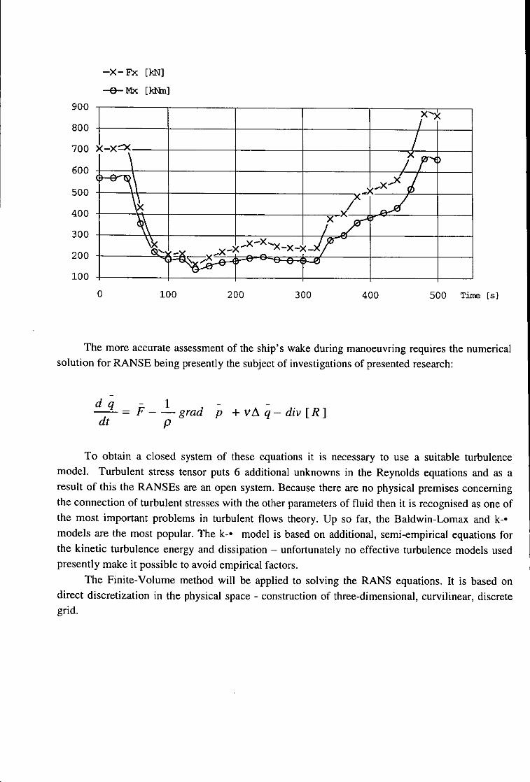
-X- Fx [kN]

-- Mx [kNM]

900 ______

800

700 X-X~ x -

600

500 /2 -

400 X

300 /"x-XxXIX

200 - .-.X X XX- -X-.

100 ___ _ _-_

0 100 200 300 400 500 Time [s)

The more accurate assessment of the ship's wake during manoeuvring requires the numericalsolution for RANSE being presently the subject of investigations of presented research:

d q Idq= F- grad p +vAq-div[R]dt p

To obtain a closed system of these equations it is necessary to use a suitable turbulencemodel. Turbulent stress tensor puts 6 additional unknowns in the Reynolds equations and as aresult of this the RANSEs are an open system. Because there are no physical premises concerningthe connection of turbulent stresses with the other parameters of fluid then it is recognised as one ofthe most important problems in turbulent flows theory. Up so far, the Baldwin-Lomax and k-omodels are the most popular. The k-° model is based on additional, semi-empirical equations forthe kinetic turbulence energy and dissipation - unfortunately no effective turbulence models usedpresently make it possible to avoid empirical factors.

The Finite-Volume method will be applied to solving the RANS equations. It is based ondirect discretization in the physical space - construction of three-dimensional, curvilinear, discretegrid.

Convergence Study of Viscous Flow Computations Around a High Loaded NozzlePropeller

Moustafa Abdel-Maksoud 1, Potsdam Model Basin

Nozzle propellers are an ideal propulsion system for many marine applications such as fishing and tug boats,dynamic positioning of platforms, etc. The operation conditions for these applications are high thrust loadingcoefficients (C~h) and low propeller inflow velocities (V.). In this case, high loaded nozzle propellers are is muchmore efficient than conventional ones. Nozzle propellers have many advantages. The contraction of the flow throughthe nozzle reduce the inhomogenity of the propeller inflow. High thrust loading can be achieved along the propellerblade also near the tip. The pressure reduction of the flow Mround the nozzle produces an additional thrust. The ratioof the nozzle thrust to the propeller one increases with increasing the thrust loading coefficient. The thrust of thenozzle may be exceed the propeller thrust at bollard pull conditions.

The accuracy of the results of the numerical calculation is effected by the accuracy of the simulation of the flow inthe gap between the propeller tip and the inside wall of the nozzle. With increasing the thrust loading, the influenceof this gap will be strongly increased. In model scale this gap could be less than one millimetre. The application ofRANS method for the prediction of the flow around nozzle propellers has many advantages. More detail informationon the flow can be captured than in the experiment, e.g. the velocity and pressure distribution on the propeller bladesand on the nozzle. Unfortunately, the required computational effort increases rapidly when the thrust loadingcoefficient increases. The combination of the experimental and numerical investigations can overcome the short-coming of each method. The experimental data can give a good overview on the forces and moments for the wholerange of operational conditions. The numerical computations can be applied to focus the detail of the flow forselected loading conditions.

The increasing of the thrust loading means also the increase of the ratio between the circumferential and axialvelocity components of the propeller flow. Close to the bollard pull condition, where the propeller inflow velocity isnearly zero, this ratio and the thrust loading coefficient go to infinity. For CTh>lOOO, the increase of the axial velocitycomponent behind the propeller may be more than 30 times of the inflow velocity. At the begin of the experiment,when the propeller starts to rotate, the axial velocity component is still very low, the thrust loading of the propeller isextremely high and the produced nozzle thrust is very low. With acceleration of the flow due to the propeller actionthe thrust loading of nozzle is increased and the propeller loading is decreased.

The computation of the viscous flow for a nozzle propeller is more complicated than for a conventional one.Convergence problems should be expected due to unsteady behaviour of the problem and the large differencebetween the inflow velocity of the computational domain and the inflow velocity of the propeller. The first isindependent of the simulation time t1, the second one is strongly depending on it. In addition, the total thrust and theratio between the propeller and the nozzle thrust are effected also by the simulation time. Many other factorsinfluence the convergence behaviour negatively, e.g. the high number of revolutions of the propeller and the smallgap between the propeller and nozzle.

The numerical computations of the viscous flow were carried out for a four blade nozzle propeller. One propellerblade is considered in the computations. The calculation domain is a quarter of a cylinder. On the sides of thecomputational domain a periodic boundary condition is applied to consider the influence of the other blades. Thecalculation domain is divided into a stationary part and a rotating one. The stationary part includes the inflow andoutflow regions and the nozzle. The propeller blade and a part of the propeller shaft are included in the rotating partof the computational domain. In the stationary part a Cartesian co-ordinate system is employed. The flow around thepropeller is computed in a rotating co-ordinate system attached to the propeller. The number of revolutions and theinflow velocity are kept constant during the computations. The RANS equations in a rotating co-ordinate systeminvolve additional terms compared to those in an inertial system. The computations were carried out with thecommercial CFD software package CFX-TASCflow of AEA Technology. CFX-TASCflow uses a Finite Elementbased Finite Volume method. It uses block-structured non-orthogonal grids with grid attachment to discretise thedomain. CFX-TASCflow models the equation for the conservation of mass, momentum and energy in terms of thedependent variables velocity and pressure in their Reynolds averaged form. The variables are discretised on a co-located grid with a second order fully conservative vertex based scheme. In the computations the "Linear Profile"

Potsdam Model Basin, Marquardter Chaussee 100, 0-14669 Potsdamn, Maksoud@sva-potsdam.de

scheme with "Physical Advection Correction" of Schneider and Raw [I] was applied. The resulting linear equationsystem is solved with an Algebraic Multi-Grid (ANG) solver, which shows a linear scalability of the code with thenumber of grid cells. The equations are solved fully coupled.

Two turbulence models were applied in the present investigation, the standard k-E model with a scalable wallfunction and advanced k-co based model for improved separation prediction (SST model [2]). All formulations usedin this study use a scalable near wall treatment, which allows a consistent grid refinement near the wall [3]. Specialattention was paid to the stagnation point problems of two-equation models, using the Kato-Launder [4] modificationor a production term limiter [2] for the k-cu based models.

The code was optimised and intensively tested for propellers in uniform flow and for behind ship condition. Theinvestigations were carr ied out within a joint research project between the Potsdam Model Basin GmbH and AEATechnology GmbH, supported by the German Ministry for [Education, Research and Technology [5]. The numericalmethod includes fully conservative stage capabilities to simulate the interaction of the nozzle and the propeller. Non-matching sliding grid interface is applied at the interfaces between the numerical grids in the rotating and thestationary frame.

The computations were carried out for model scale. A 3D solid CAD model was used for the grid generation. Thegeometry of the propeller blade and of the nozzle were considered without simplification. The gap between them wasalso included in the computation. Two different numerical grid configurations were applied. The first one consistedof 15 blocks and 320,000 control volumes. In the second grid approximately twice number of blocks and controlvolumes were used, Fig.1I.

The investigation was carried out for many thrust loading coefficients. The results of 5 computations for the thrustloading coefficient 1000 will be discussed and compared with the measured results. Table I summarizes the resultsfor the thrust and torque coefficients. The computations were carried out for different dimensions of the computationdomain and turbulence models. The topology of the numerical grid and grid resolution were also varied, Table 1. Dpis the propeller diameter, The simulation time (twas at least 30 seconds for each test case.

In the first test case, the calculated thrust of the propeller and the nozzle were lower than the measured values,specially the nozzle thrust is too low. In test case 2, the effect of the dimensions of the computational domain on thenumerical results was investigated. The location of the outlet was moved from 6.5 to 20 Dp behind the propeller. Thediameter of the computation domain D. was also increased from 4 to 9 Dp. The results show that the calculatedthrust of the propeller and the nozzle are much higher than the corresponding values for case 1, specially the nozzlethrust, Table 1. At Cn,=l000 the axial velocity component in the propeller slip stream is much higher than the axialvelocity component of the flow surrounding it. The high velocity gradient causes a re-circulation region and backflow may occur near the outlet region. That was the case for the second test case.

The dimensions of the calculation domain were increased again to avoid the back flow problem at the outlet, see testcase 3. The distance between the propeller plane and of the inflow and outflow planes were increased to 87, 130.5Dp respectively. The diameter of the calculation domain was also increased to 90 Dp. The numerical results of thistest case show that the calculated propeller and nozzle thrust were increased. The calculated propeller thrust and thecalculated ratio of propeller thrust to propeller torque are much higher than measured.

In test case 4, the effect of the turbulence model on the results of case 3 was investigated. The SST turbulence modelcan predict flow separation better than the standard k-e model with wall function. Therefore, the SST turbulencemodel was applied in case 4 reducing the differences between the measured and calculated propeller thrust werereduced. This confirms that a good predication of the flow separation is important to calculate the flow on thepropeller blade at high loading coefficient.

The y* values used in the first grid, used in cases I to 4, were not optimum for application of the SST model.Therefore a new grid was generated using the double grid resolution near the walls. The results with the test case 5show that the thrust of the nozzle and the propeller are well predicted. The calculated propeller torque coefficient andthe ratio of total thrust to the propeller torque agree well with the measured values. In addition, good convergencebehaviour was achieved.

In the following some aspects of the nozzle propeller flow will be focused. The presented results are for test case 5.Figs. I and 2 show the streamlines of the propeller inflow. The contraction of the flow in the front of the propeller isvery high and there is back flow near the leading edge of the nozzle.

The unsteady behaviour of the nozzle propeller can be divided into two stages. The duration of first stage is aboutone second. In this stage the propeller trust is increased rapidly in the first 0.15 seconds. With increasing the nozzlethrust, the propeller thrust is decreased, Fig.3. The duration of the second stage is about 25 seconds, Fig.4. In thisstage the propeller thrust is nearly constant and the nozzle thrust is increased very slowly. Concerning theconvergence behaviour, the first 0.1 second is the most critical phase of the simulation.

Figs.5-8 show the velocity vectors in the most important regions of the computation. Fig.5 shows the flow outsidethe nozzle. Due to the lack of the axial flow, the propeller gets its inflow from its surrounding. The stagnation pointis located at the middle of the nozzle where the flow is divided into two regions. The first one flows toward theleading edge and the other one toward the trailing edge. Fig.6 shows the velocity vectors at the leading edge. Due tothe suction effect of the propeller, the velocity of the propeller inflow increased rapidly in this region. Fig.7 showsthe flow at the trailing edge of the nozzle. The velocity vectors of the flow inside the nozzle are much higher than theflow outside it resulting in a very high velocity gradient in this region. Fig.8 shows the flow in gap between propellerblade and nozzle with a tip vortex on the propeller blade and back flow on the inside wall of the nozzle.

References

[1] Schneider G. E. and Raw, M. J., Control Volume Finite Element Method for Heat Transfer and Fluid Flow usingCo-located Variables, Numerical Heat Transfer, Vol. 11, pp. 363-390, 1987.

[2] Menter F. R., Two-Equation Eddy-Viscosity Turbulence Models for Engineering Applications, AIAA- Journal,Vol. 32 (8), pp. 269-289, 1994.

[3] Grotjans, H. and Menter F. R. Wall Functions for Industrial Applications, In Papailiou, K. D. Editor,Computational Fluid Dynamics 98, Volume 1, Part 2, pp. 1112-1117, Chichester, 1998, ECCOMAS, John Wiley& Sons.

(4] Kato, M. and Launder B. E., The Modelling of Turbulent Flow around Stationary and Vibrating Cylinders, InNinth Symposium on Turbulent Shear Flows, Kyoto, Japan, 1993

[5] Abdel-Maksoud, M., Menter, F. R., Wuttke, H.: Numerical Computation of the Viscous Flow around the Series60 Ca = 0.6 Ship with Rotating Propeller, 3rd Osaka Coll.. on Advanced CFD Appl. to Ship and Hull FormDesign, Osaka, May 1998

Table 1: Summary of the numerical results and boundary conditions.

Test case 1 2 3 4 5 ExperimentPropeller thrust coeff. K-r 0.186 0.229 0.243 0.238 0.225 0.222Propeller torque coeff. 10KQ 0.363 0.387 0.372 0.365 0.381 0.373Nozzle thrust coeff. KT, 0.084 0.208 0.214 0.211 0.216 0.215Total thrust coef. K-rr 0.271 0.437 0.457 0.449 0.441 0.437KTKQ 5.127 5.925 6.539 6.537 5.896 5.960KTT/KQ 7.450 11.289 12.304 12.323 11.545 11.718KrfKrr 0.453 0.905 0.882 0.885 0.958 0.966Thrust loading coefficient CTH 621 1004 1050 1032 1012 1002DcorPp 4 9 90 90 70Location of inflow plane X/Dp 3.5 3.5 87 87 87Location of outflow plane X/Dp 6.5 22 130.5 130.5 130.5Turbulence model K-c K-c K-E SST SSTlConvergence fast. back flow slow. slow Fast

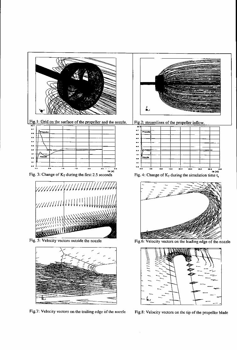
Fig. 1: Grid on the surface of the propeller and the nozzle. Fig.2: streamlines of the propeller inflow.

o l o

o - ao

° * 1 ° .s.cl- n ~

ta Is] t. fri

Fig. 3: Change of Kr during the first 2.5 seconds Fig. 4: Change of KT during the simulation time t,

Fig. 5: Velocity vectors outside the nozzle Fig.6: Velocity vectors on the leading edge of the nozzle

Fig.7: Velocity vectors on the trailing edge of the nozzle Fig.8: Velocity vectors on the tip of the propeller blade

The Effect of Non-Linear Froude-Krylov Forces on the Seakeeping of MonohullVessels Using a Novel Calculation Method

by P.A. Bailey', E.J. Ballard', D.A. Hudson' and P. Temarel'.

Introduction

A time domain mathematical model of ship motions allows for the incorporation of arbitrary and/or transientexcitation, such as the influence of control surfaces and random waves. When compared to more conventionalfrequency domain analyses of ship motions [1-3], the possible arbitrary nature of motion/excitation in a timesimulation leads to additional complications in the formulation and calculation of the forces and moments. Inessence the fluid memory effect, exemplified by the generation of motion induced surface waves, introduces adependence of the forces and moments on the past motions/excitations [4].Recent studies [5-8] have investigated the use of convolution type expressions to represent fluid forces andmoments on the ship. These expressions, applicable to arbitrary forms of linear motion/excitation, require thecalculation of impulse response functions. This has been achieved using transforms of frequency domain datafrom three dimensional Green's function seakeeping methods [9-12].It is believed by some that observed differences between theoretical linear motion predictions and experimentalresults can be attributed, to some extent, to the nature of the excitation, particularly for ships with large flare.To this end, it is possible to introduce a non-linear component of excitation into an otherwise linear system [131.Integration of the Froude-Krylov wave excitation pressure over the instantaneous wetted surface yields such acontribution, but the integration method is complicated by the changing nature of the underwater form.

Mathematical Model

Seakeeping theory has traditionally referenced rigid body motions of a vessel to equilibrium axes. However,the behaviour of frequency domain added mass and hydrodynamic damping calculated with reference to theseaxes results in problematic evaluation of the corresponding impulse response functions [5]. Recently it has beenshown by Bailey [14] that frequency domain data transformed to a set of body fixed axes is more amenable toaccurate calculation of impulse response functions. The required transformation of data is discussed in detailby Bailey et. al. [6].

The heave and pitch (z* and 0) equations of motion referenced to a right handed body fixed axis Cxyz arewritten as

[b(t) f3(w,q,z*,O,t)

where w is the heave velocity, q is the pitch angular velocity and where

f3 = Zr+Za+Zw(oo)w+2 q(oo)q+mqU

f5 = Mr+Ma+M-voo)w + Mq(oo)q.

The combination of weight, buoyancy and wave excitation actions are, for the present, denoted using terms witha subscript a. In due course, the detail of these terms will be discussed with reference to particular methods.The mass matrix is given by

M = [ _2 m - (0o) -24(oo )-A() Y- W(oo)

Terms such as R. (w,) and !f1,b (we) are the frequency dependent velocity and acceleration derivatives respec-tively, calculated by transforming seakeeping coefficients of added mass and damping to the body fixed axissystem [6]. The terms with the subscript r are the motion dependent hydrodynamnic forces and moments(radiation actions) and are expressed using the impulse response functions as follows

Zr = z,(r)w(t - r)d& + j zq(Q)q(t - r)dr

'School of Engineering Sciences, Ship Science, University of Southampton, United Kingdom.

1

M, = ftm,(w)w(t- i)dr+ Mqr)q(t - 7)d-.

For r > 0, the impulse response functions can be calculated using either the velocity or acceleration frequencydomain data [5-8), for example

z = = / (w,) cos (wgr) dw w, Zb (we) sin (w-) ,7r o 7r

The three dimensional theoretical methods used to calculate the frequency domain data in these these expressionsare discussed in detail by Duet. al. [9,111 and Bailey et. al. [10, 121.Two time simulation methods have been developed, both of which use this formulation for the radiation actionsbut which use differing formulations for the wave excitations. These two methods will be referred to as methodsA and B.

Method A: Linear Wave Excitation

It has been shown by Bailey et. al. [5] that linear wave excitation actions can be represented using a convolutiontype formulation such that terms with a subscript a in equation (1) can be represented as

Zý = zF(r)a(t - r)dr + zD ()a(t - 7-)d- + Z,.z* + ZoO

Ma = mF(r)a(t - r)dT + mD(Tr)a(t -- r)di- + M=. z* + MoO.

Here the superscripts F and D refer to the Froude-Krylov and diffraction components respectively. Calculationof these wave excitation impulse response functions is more difficult than calculation of the radiation impulseresponse functions, since the influence a wave has before it reaches the reference must be accounted for. Effec-tively, the wave excitation impulse response functions are non-zero for T < 0 [5, 15], and unlike the radiationimpulse response functions their calculation requires both the real and imaginary parts. For example,

zj{R(we) cos(weT) - =l(we) sin(wer)}dw, for all r.

Method B: Non-Linear Froude-Krylov

In this method, the terms in equation (1) denoted with a subscript a represent non-linear restoring and Froude-Krylov forces and moments. In order to calculate these terms, a method of determining the buoyancy andFroude-Krylov wave excitations up to the incident waterline with the ship in its perturbed state has beendeveloped. The non-linear Froude Krylov and restoring forces and moments are then calculated by subtractingthe relevant components of weight.

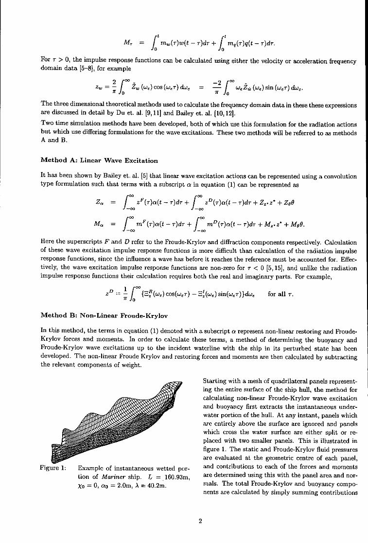
Starting with a mesh of quadrilateral panels represent-ing the entire surface of the ship hull, the method forcalculating non-linear Froude-Krylov wave excitationand buoyancy first extracts the instantaneous under-water portion of the hull. At any instant, panels whichare entirely above the surface are ignored and panelswhich cross the water surface are either split or re-placed with two smaller panels. This is illustrated infigure 1. The static and Froude-Krylov fluid pressuresare evaluated at the geometric centre of each panel,

Figure 1: Example of instantaneous wetted por- and contributions to each of the forces and momentstion of Mariner ship. L = 160.93m, are determined using this with the panel area and nor-

Xo = 0, ao = 2.0m, A = 40.2m. mals. The total Froude-Krylov and buoyancy compo-nents are calculated by simply summing contributions

2

from all the panels.

In the development of this scheme, great care has been taken to ensure that splitting, adding or destroyingpanels as the motion progresses does not introduce step changes in the resulting forces and moments [141.At present, this method excludes any contribution from the diffraction wave excitation.

Results and Discussion

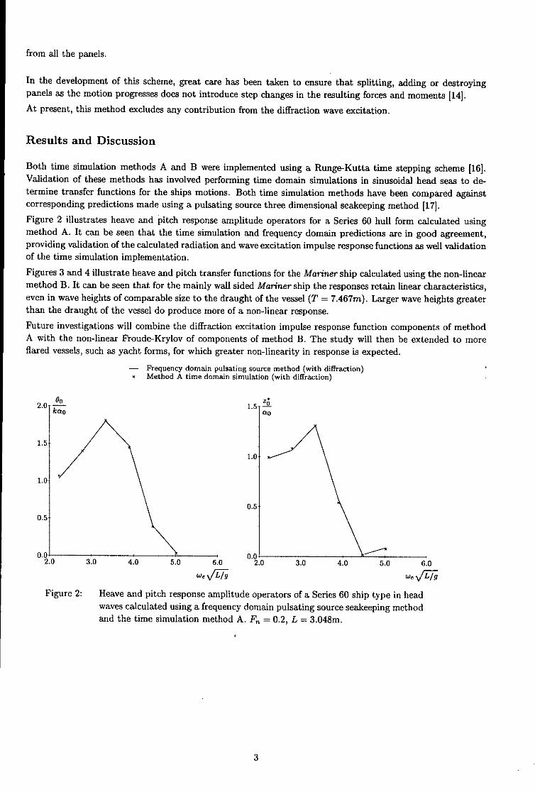
Both time simulation methods A and B were implemented using a Runge-Kutta time stepping scheme [16].Validation of these methods has involved performing time domain simulations in sinusoidal head seas to de-termine transfer functions for the ships motions. Both time simulation methods have been compared againstcorresponding predictions made using a pulsating source three dimensional seakeeping method [17].Figure 2 illustrates heave and pitch response amplitude operators for a Series 60 hull form calculated usingmethod A. It can be seen that the time simulation and frequency domain predictions are in good agreement,providing validation of the calculated radiation and wave excitation impulse response functions as well validationof the time simulation implementation.

Figures 3 and 4 illustrate heave and pitch transfer functions for the Mariner ship calculated using the non-linearmethod B. It can be seen that for the mainly wail sided Mariner ship the responses retain linear characteristics,even in wave heights of comparable size to the draught of the vessel (T = 7.467m). Larger wave heights greaterthan the draught of the vessel do produce more of a non-linear response.

Future investigations will combine the diffraction excitation impulse response function components of methodA with the non-linear Froude-Krylov of components of method B. The study will then be extended to moreflared vessels, such as yacht forms, for which greater non-linearity in response is expected.

- Frequency domain pulsating source method (with diffraction)xMethod A time domain simulation (with diffraction)

2.0 00 1.5 Z.ka0 on

1.5

1.01.

0.50.5

0.0- 0.0 -2.0 3.0 4.0 5.0 6.0 2.0 3.0 4.0 5.0 6.0

Figure 2: Heave and pitch response amplitude operators of a Series 60 ship type in headwaves calculated using a frequency domain pulsating source seakeeping methodand the time simulation method A. F, = 0.2, L = 3.048m.

3

- Frequency domain pulsating source method (with diffraction)---. Frequency domain pulsating source method (without diffraction)

Method B time domain simulation (without diffraction)*10-2 Go )

5 .0T 00 (m--l) , 1.5 z

e

anon

4.0 ,. /

1.0~3.0

2.0

0.5

0.0 0.00.0 2.0 4.0 6.0 8.0 10.0 0.0 2.0 4.0 6.0 8.0 10.0

Figure 3: Heave and pitch transfer functions of Mariner ship type in head waves caJ-culated using a frequency domain pulsating source seakeeping method andthe time simulation method B. F. = 0.19, L = 160.93m, wave amplitude~o =0.01m.

- Frequency domain pulsating source method (with diffraction).... Frequency domain pulsating source method (without diffraction)

Method B time domain simulation (without diffraction)*10-2 1. Z;

. (m- 1 ) 1.

4.0'K

1.03.0

2.0

0.5

1.0

0.0 0.0 , ,0.0 2.0 4.0 6.0 8.0 10.0 0.0 2.0 4.0 6.0 8.0 10.0

Figure 4: Heave and pitch transfer functions of Mariner ship type in head waves cal-culated using a frequency domain pulsating source seakeeping method and thetime simulation method B. F, = 0.19, L = 160.93m, wave amplitude ao = 2.Om

References

[1] R. F. Beck, W. E. Cummins, J. F. Dalzell, P. Mandel, and W. C. Webster. Principles of Naval Architecture,volume 3, chapter 8. Trans. SNAME, 1989.

[2] J. N. Newman. Marine Hydrodynamics. MIT Press, 1977.

[3] 0. M. Faltinsen. Sea Loads on Ships and Offshore Structures. Cambridge Ocean Technology Series.Cambridge University Press, 1990.

4

[4) R. E. D. Bishop, R. K. Burcher, and W. G. Price. The fifth annual Fairey Lecture: on the linear repre-sentation of fluid forces and moments in unsteady flow. Journal of Sound and Vibration, 29(1):113-128,1973.

[5] P. A. Bailey, E. J. Ballard, D. A. Hudson, and P. Temarel. Time domain analysis of vessels in wavesaccounting for fluid memory effects. In To be published in Proc. NAV'2000, Viena, 2000.

[6] P. A. Bailey, W. C. Price, and P. Temarel. A unified mathematical model describing the manoeuvring ofa ship travelling in a seaway. Trans. RINA, 140:131-149, 1998.

[7) P. A. Bailey, D. A. Hudson, W. G. Price, and P. Temarel. Theoretical and experimental techniques forpredicting seakeeping and manoeuvring ship characteristics. In RINA Intl. Conf. on Ship Motions andManoeuvrability, Paper No. 5, London, 1998.

[8] P. A. Bailey, D. A. Hudson, W. G. Price, and P. Temarel. The measurement and prediction of fluid actionsexperienced by a manoeuvring vessel. In Proc. Intl. Symposium and Workshop on Forces acting on aManoeuvring Vessel, MAN '98, pages 117-123, Val de Reuil, France, 1998.

[9] S. X. Du, D. A. Hudson, W. G. Price, and P. Temarel. Comparison of numerical evaluation techniques forthe hydrodynamic analysis of a ship travelling in waves. Trans. RINA, 141, 1999.

[10] P. A. Bailey, D. A. Hudson, W. G. Price, and P. Temarel. Theoretical validation of the hydrodynamics ofhigh speed mono- and multi- hull vessels travelling in a seaway. In PRADS '98: The Seventh InternationalSymposium on Practical Design of Ships and Mobile Units, pages 567-576, The Hague, September 1998.Elsevier Science, B.V.

[11] S. X. Du, D. A. Hudson, W.G. Price, and P. Temarel. A validation study on mathematical models of speedand frequency dependence in seakeeping. Proceedings of the Institution of Mechanical Engineers, Part C,"214:181-202, 2000.

[12] P. A. Bailey, D. A. Hudson, W. G. Price, and P. Temarel. Comparison between theory and experiment ina seakeeping validation study. (accepted for publication). Trans. RINA, 2000.

[13] N. Fonseca and C. Guedes Soares, editors. Marine, Offshore and Ice Technology, chapter Time domainanalysis of vertical ship motions, pages 225-242. Computational Mechanics Publication, 1994.

[14] P. A. Bailey. Manoeuvring of a ship in a seaway. PhD Thesis, University of Southampton, 1999.

[15] B. K. King, R. F. Beck, and A. R. Magee. Seakeeping calculations with forward speed using time-domainanalysis. In 17th Symposium on Naval Hydrodynamics, pages 577-596, The Hague, The Netherlands, 1988.

[16] S. Nakamura. Applied Numerical Methods in C. Prentice Hall, 1993.

[17] R. B. Inglis. A Three Dimensional Analysis of the Motion of a Rigid Ship in Waves. PhD thesis, Universityof London, 1980.

5

Post-Processing of Time-Dependent CFD Analyses using Virtual Reality Modelling Language

Marco Barcellona, INSEAN, Via di Vallerano 139, 1-00128 Rome, marco@rios3.insean.itVolker Bertram, HSVA, Branifelder Str 164, D-22305 Hamburg, bertram@hsva.de

The predominant CFD application today is the simulation of resistance and propulsion tests, i.e. thecomputation of the flow about a ship moving steadily ahead with constant speed. However, research isactive on unsteady flow simulations, namely seakeeping and maneuvering simulations. A naturalextension of current 'snap-shot' plots are animations or - one step further - Virtual Reality animationsallowing customers to browse arbitrarily through flow fields in time and space. We use here the term"Virtual Reality" for the "poor man's" version of Virtual Reality, i.e. a usually mouse-controllednavigation through a three-dimensional environment on a graphics monitor. This is far from what fullyimmersive Virtual Reality envisions, but can be realized on computer hardware widely available inindustry and is sufficient for the applications we have in mind.

Most CFD applications in naval architecture involve dedicated hydrodynamic experts consultingshipyard designers. The consultants are usually at some other location than the customers. Ideally, wewould like to have a commercial-of-the-shelf (COTS) visualization tool capable of producing'unlimited' or 'continuous' views in space and time, with the ability to 'zoom' in space or time (slow-motion). The models should be easily communicated via the web and should be readable for customerswithout requiring significant investment in hardware and software, preferably running on 'plain-vanilla' PCs. Ideally, software should be public domain and be available in both Windows and Linuxversions. The Virtual Reality Modeling Language VRML supports these requirements to a largeextent. The language is worldwide ISO/IEC standard in the version of VRML 2.0 and standardbrowser to view the models can be downloaded from the internet. Inclusion in websites isstraightforward and customers could e,g. access models via internet. Confidentiality can be protectedby passwords. VRML like any other programming language has a relatively simple set of commandsand structures. However, the creation of 'Virtual Reality' models is cumbersome for practicalapplications. In addition, tailor-made interfaces have to be written for CFD programs used. The effortand expense in writing these should not be underestimated, but this is largely a once-time, initialinvestment. A simple interface may be written in half a day. Such interfaces are readily converted toother CFD program formats and sharing the burden with other users may lower the threshold of using'Virtual Reality' in practice.

After an initial phase of getting acquainted with VRML in studying similar applications available onthe internet in simple tutorials and the website of the VRL of the University of Michigan (www-URL.umich.edu), we applied 'Virtual Reality' to projects of our own, Barcellona and Bertram (2000):

Our first application concerns a multi-body structure in current and waves. The particular study wasfor a mobile offshore base (MOB) structure and submarines configuration of the Italian navy. Thisstationary platform moving in a seaway can be regarded as a representative of typical applications inoffshore engineering. The application is relatively complex involving the following 'advanced'features:complex body shapes (the actual confidential shape is complex, we show simplified generic structures)o time as 4th dimensiono free surfaceo multiple degrees of freedom in the time simulation, to be correctly routed with timer and event-

generation mechanismMoreover, a small tool had to be developed to correctly combine Eulerian rotations in single axisrotation, and then rewritten in the VRML-understandable format, i.e. a vector and an angle (positive inclockwise direction). Such tools are freely available on the web, but they are not intended to deal withhuge amounts of data, necessary for a time simulation.

The second application concerned a trimaran in irregular waves. The region between outrigger andmain hull is usually bidden from a side view and the ability to fly at will through the model and turnthe perspective quickly is useful even for steady flow applications. The 'advanced' features of thismodel are:* body of complex shape* time evolution of pressure on bull* free surface

People who want to create advanced VRML models will have to learn the language despite contraryclaims by vendors of VRML editors. You can indeed create simple Virtual Reality models using thesetools without any knowledge of the VRML syntax. However, reality is seldom that simple. Ourapplications involved aspects that were practically impossible to include by using such editors:

1. CED simulations in time require also VRML time simulations. Editing and authoring tools as the'animation wizard' of Spazz3d are so far too limited in their 'wizardry'. They do not allow toprescribe an arbitrary motion for an object by giving a set of non-uniformn points in time withrelated sets of rotations and translations to generate automatically an interpolated animation. Evenif this were possible the user must have at least a profound knowledge about the format in whichdata have to be stored. The routing process, i.e. the mechanism by which the browser connecttimers processes, is not trivial, especially if you need to add time-evolving processes to beinteractively started and stopped during the 'navigation' across the virtual world.

2. The VRML model exported by a VRML editor like Spazz3d contains many complex, deeplynested, repeated stmuctures. It may be seen as roughly comparable to a Fortran or C codegenerated by a mathematical manipulation shell like Maple. It works, but it is very difficult tounderstand and thus to modify or extend. For our CFD visualization problems, we wereconfronted with megabytes of CFD data at each time instant. The velocity of the parser and thebrowser during the analysis of these structures strongly affect the reliability and the level of'reality' of the simulation. Thus, the automatically generated models by a VRML authoring toolneed often to be 'optimized' to run fast enough on a PC. Data reduction is also desirable forsending VRML files across the web. Again, the minimum-size format (browsers are also capableto read gzipped worlds) is in conflict with the requirements of cleaniness and readability, tomodify and debug the world. A common situation is that one wants to create in principle identicalworlds with different data sets. This implies reopening the code by the graphic VRML editorlosing time to reload the new sets. A simple C, FORTRAN, or PERL program or script could dothe work simpler and much faster, even in a non-graphic environment.

3. A very complex, storage-demanding grid can be imported automatically in the Virtual Realitymodel only if it has the right format. Many commercial grid generators include in their newestreleases VRML import/export facilities for this purpose. However, individual grid generators stillpopular in the marine CFD community require custom-made programming to interface to VRML.

4. Typically, CFD simulations involve huge amounts of data in the output. Time simulations requirea sometimes very small time steps to prevent the numerical scheme from instabilities. The humaneye does often not require such a high resolution in time in an animation. Timers in VRML areobject that can be activated by signals and retrieves a value (boolean, real and so on) for each call.One of the basic features in VMRL is that at each timer signal (event) the routed processes(=connected with the timer) perform an interpolation (PositionInterpolator,Orientationinterpolator, CoordinateInterpolator etc.) between the last and the actual status, thusallowing the user to clean up the data set by purging several unnecessary (for the animation)configurations. This results in a considerable reduction of the data size. This we call 'dataoptimization in time'. Similarly, the spatial resolution in CED grids is often much finer thanrequired for the animation. Simple objects like boxes, cylinders and spheres are built-in in thebrowser and, even if it must perform triangularization and 3D-rendering process to represent them,it does the work in a simpler and faster way, saving considerable time and memory.

There is a clear learning curve as with any software. The first application of the multi-body systemtook approximately 10 days to develop, the second application of the trimaran only approximately 5

days, mostly spent in building suitable FORTRAN and PERL tools to convert and recast data inVRML-accessible format. An experienced user may be able to create such models in a fraction of thetime we needed. Generally, the time needed depends upon the desired degree of 'reality'. Based on ourexperience, we can recommend to newcomers to 'Virtual Reality' for CRD:o get the complete VRML ISO/IEC specification* get some VRML tutorials to have an overview of the topic, of the results you can obtain, and the

effort it takes.o get a complete VRML 2.0 handbook for referenceo learn by modifying examples; many commands and structures are unnecessary for your

applicationo establish a network to colleagues working on similar applications and share experience and

macros* count on several days before you have a model that satisfies you in the initial stage* a background in object-oriented languages like C++ helpso get a dedicated PC and use Windowso add complexity gradually in creating large 'Virtual Reality' models" make the model only as complex as it needs to be; 'cosmetics' can be expensive

'Virtual Reality' models are in many ways like traditional CAD models. Initial model creation iscumbersome, but model modification is relatively fast. Thus 'Virtual Reality' model designers willtypically start collecting a 'database' of models and, after a while, especially if there are essentiallyalways the same applications, be quite fast in creating such adjusted models. Sharing models withcolleagues should accelerate the process of setting up a set of 'parent' applications which only need tobe modified to particular projects.

BARCELLONA, M.; BERTRAM, V. (2000), Virtual Reality for CFD Post-Processing, COMPIT,Potsdam

VRML models: www. schif fbau.uni-hamburg.de/IFS/AB/AB-3-14/VR/

VRML model of Mobile Offshore Base VRML model of trimaran

STEADY AND UNSTEADY COMPUTATIONS OF SHIP FLOWSIN A STRAIGHT CHANNEL

Marco Barcellona*, Giorgio Graziani, Maurizio Landrini*

* INSEAN, The Italian Ship Model Basint Dipartimento di Meccanica e Aeronautica, Universitd di Roma "La Sapienza"

The growing interest for fast transportation in natural and artificial inland channels calls for theanalysis of the related problems, like possible damages to shores and moored floating structures, dropof the efficiency of vessels and safety aspects (Bertram et. al. 1999, Yasukawa 1999). In this paper wepresent our first attempts to predict numerically forces and wave pattern associated with the motion ofa vessel in a channel. A well established potential flow model is considered and the problem is solvednumerically by a boundary integral method. For straight channels, a suitable Green function is usedand only the free surface and the hull boundary have been discretized. Preliminary results for steady,symmetric flows are reported. An extended set of results will be discussed at the workshop.

1 MATHEMATICAL MODEL For numerical purposes, the potential is repre-sented by a distribution of sources and dipoles, theIn the following, the flow around a hull advanc- latter being introduced to enforce a Kutta condi-

ing with speed V(t) is studied by a potential flow tion along the stern line in case of non-symmetricmodel. A frame of reference moving with the ship flows. In short, the velocity potential in the pointis considered, with x-axis aligned with the ship P can be written asmotion and the vertical axis opposite to the grav-ity direction. The y-coordinate spans across the (P(P) = [ty + -TB + 'bottom + Zlat w.1channel. The considered fluid domain includes aportion of the channel OflbottomUl .lat wn, the hull wheresurface 8flB and the free surface Ofty. The total Zy = ff ayrG(x,P)dS (2)velocity of the fluid is written as JJis the influence of the free surface andU(P, t) = -V(t) + u'(P, t) = -V + Výo(P, t) 1 f +G

where the perturbation velocity u' is described in 5n = aG(x, P)dS + P)dSterms of the velocity potential Vp. The latter sat- (3)isfies the Laplace equation V2rp = 0, the no pene- is the influence of the body. The dipoles are dis-tration boundary condition tributed over a fictitious surface B1 inside the hull

and along a trailing wake of zero thickness.(V + V'o) -nB = 0 on Q5 The influence of the channel (bottom and lat-

eral walls) is computed by mirror images. It ison the surface of the moving vessel, and the kine- worth noticing that for the lateral walls, an infi-matic nite series of images should be used. To reduce the

y, t) computational effort, a fast summation algorithm+ (-V + VWp) - V1 = Oz (1) due to Breit (1991) is here adopted. This imply

the use of a modified Green function in integralsand dynamic (2)-(3).

DnW 1 The relevant integral equations are obtained byDt 2 IV2 I + gr = const collocating on the hull and on the free surface and

are discretized by a collection of flat panels. Influ-boundary conditions on the free surface. ence coefficients are evaluated by a combination of

In principle, the above formulation is gener- analytical formulas (Hess & Smith, 1965) for theally valid for the unsteady, nonlinear, nonbreak- singular part of the Green function, and of nu-ing case. In this preliminary study, the problem merical quadratures (Lyness & Jespersen ,1975),is linearized with respect to the unperturbed free for the non singular contribution. An alterna-surface configuration (z = 0, Vx, y) and the hull in tive desingularized algorithm on the free surfaceeven keel conditions. (Bertram, 1990, Cao et al., 1991) has also been

tested, with a significant reduction of the cpu-time where two different discretizations of the computa-requirements. tional domain are considered. The length is taken

The time stepping procedure, based on a fourth- 7.OLpp in the first case and 3.5Lpp in the second,order Runge-Kutta scheme, can be summarised as Lpp being the hull length between the perpendic-follows: ulars. The channel is 1.5Lpp broad, the speed is

1. for a given time to, a b.v.p. of the form = 0.22.For the same channel width, figure 2 shows the

v = 0 effect of the Froude number F.. Here, the maxi-mum number of elements on the free surface (for

I the lowest F.) is 150x32, that gives approximately(V + V~p]s ) • nB = 0 8 panels per wavelength at F. = 0.2. In the up-(v + Vo1•B1) -nB, = 0 per plot a comparison between the wave cuts in

Kutta condition proximity of the channel boundary is shown.Finally, a preliminary example of unsteady com-

is solved by the panel method above. putations is given by considering a source/sinkpair, aligned with x-axis, moving below the free

2. a new set of boundary data is determined by surface. The choice for the relevant parameters isstepping forward in time the evolution equa- made with the aim to mimic the disturbance duetions to a slender hull. Upon assuming Lpp = 1 and

V= -49 (4) the draught d = 0.0625Lpp, the distance between49X source and sink is 0.877Lpp, and they are placed

symmetrically around (0.0, 0.0, -d/2).K2o To reduce transient effects, the strength ao

8z - g Ox 2 VýAý, Aý being the cross sectional area near mid-ship. In particular, the law a(t) = ao(l - e-4t) isAlternatively, the kinematic equation (1) can be used. The same law is assumed for the dimension-

rewritten as less speed F.(t) of the pair.

a~ v, . V• 2a2 Plots in figure 3 show the time evolution of the77 = Wz - - y Ox2 free surface. The domain considered here is 6.01,

broad. The upstream extent of the computationalwhich avoids the need to compute OtI/Olx but im- domain depends on the need to minimize possi-plies the solution of an extra integral equation ble reflections of long starting waves. The down-for @. This second approach does not increase stream extent is related both the length of the ad-the computational effort and allows to handle eas- sorbing beach and to far field nedeed, for exampleily unstructured free surface grids. On the other for wave wash prediction. In particular, for thehand, this scheme suffers more stringent stability selected F., 90 x 20 panels are distributed over arequirements than the previous one and a system- computational free surface with length of 15Lpp.atic use of free surface filtering and smaller timesteps are needed. Results and performances fromboth algorithms will be discussed.

In any case, a numerical beach (Israeli and 3 FURTHER DEVELOPMENTSOrszag, 1981) is used to prevent unphysical re-flection from the truncated boundaries. At the workshop some results concerning the un-

steady, linearized and non-symmetric case of a hull2 PRELIMINARY RESULTS moving in a straight channel will be presented.

The numerical algorithm has been already devel-To gain some confidence with the problem in con- oped and validated using some simple test casesfined water, we first considered the motion of a (i.e. moving singularities). Results from the lin-Wigley hull under the assumption of steady state earized code have been compared with those fromconditions and symmetric flow. a nonlinear algorithm, giving a reasonable agree-

In this case, the radiation condition is enforced ment.shifting upstream the collocation points. The in- Our final goal is to build an efficientfluence of the rear extent of computational domain tool to handle unsteady interactions be-seems to be quite negligible, as shown in figure 1, tween moving bodies in restricted water.

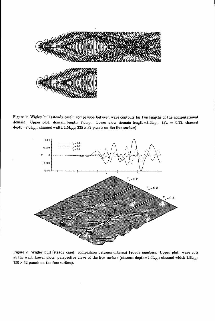
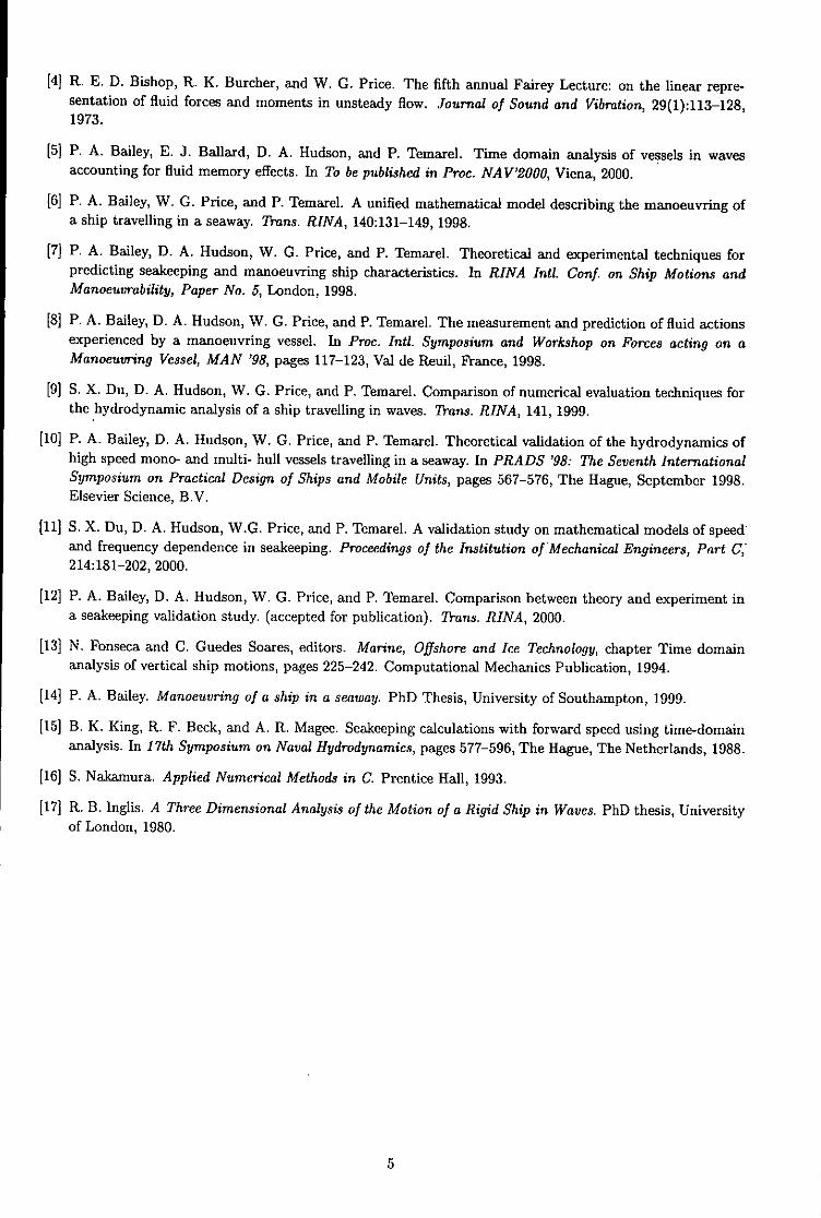
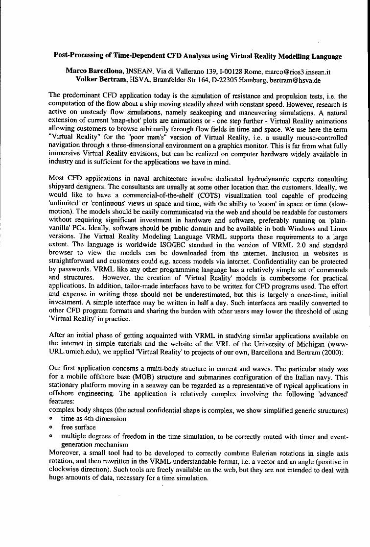
Figure 1: Wigley hull (steady case): comparison between wave contours for two lengths of the computationaldomain. Upper plot: domain length=7.0Lpp. Lower plot: domain length=3.5Lpp. (F, = 0.22, channeldepth=2.0Lpp; channel width 1.5Lpp; 225 x 32 panels on the free surface).

0.01-- Fý = 0.4

.......--- Fý - 0.3 ,0.005

V 0 --.

-0.005

-0.010x

Frn 0.3 Fý0.

Figure 2: Wigley hull (steady case): comparison between different Froude numbers. Upper plot: wave cutsat the wall. Lower plots: perspective views of the free surface (channel depth=2.OLpp; channel width 1.5Lpp;150 x 32 panels on the free surface).

BIBLIOGRAPHY 4 t- 0.20

3-

2-

BERTRAM, V., BULGARELLI U. (1999) Nu- ,merical wash prediction, First Int. Conf. on D:

High-Performance Marine Vehicles (HIPER '99),Zevenwacht, South Africa.

3-

BERTRAM, V. (1990) A Rankine source method 2:

for forward-speed diffraction problem, Report No.508, IFS, university of Hamburg, June.

4 t 1.8s

BREIT, S.R., (1991) The potential of a Rankine 3Source between parallel planes and in a rectangu- 2 -lar cylinder, Journal of Eng. Math., 25, 151-163. 1

CAO, Y., SCHULTZ, W. W., BECK, R. (1991),Three-dimensional desingularized boundary inte- ' t 2.70s

gral methods for potential problems, Int. J. Num.Meth. Fluids, Vol. 12, 785-803.

ISRAELI, M., ORSZAG, S. A. (1981), Approx- 'imation of radiation boundary conditions, J. 4:

Comp. Phys., Vol. 41, pp. 115-135. 3

2

LONGUET-HIGGING, M. S., COKELET,E. D. (1976), The deformation of steep surfacewaves on water. I. A numerical method of compu-tation, Proc. Roy. Soc. Lond., Vol. 350, pp. 1-26. ' 1.4.509

LYNESS, J.N., JESPERSEN, D. (1975), Moder-ate Degree Symmetric Quadrature Rules for theTriangle, Inst. Math. Appl. 15, 19-32.

Figure 3: Evolution of the wave pattern generated by aSMITH J., HESS A.M.O. (1965), Calculation of source/sink pair accelerating from rest up to the finalnon-lifting potential flow about arbitrary bodies, speed F. = 0.6.Prog. Aero. Sci. 8,1-138.

YASUKAWA, H. (1999) Unsteady wash computa-tion for a high speed vessel 2nd Num. TowingTank Syrup. (NuTTS 1999), Rome.

CFD in Ship Design - Some Recent Advances

Volker Bertram, HSVA, bertram@hsva.de

The applications given here will be explained in more detail in Bertram et a]. (2000). Here I selectedsubjectively some applications from previous experience that seemed to highlight particularly wellhow we use now CFD to support ship design - or how we may use it in the very near future. Theapplications are taken from HSVA's practice, but I believe they reflect in many cases the general stateof the art of other first-class CFD providers in the marine industry.

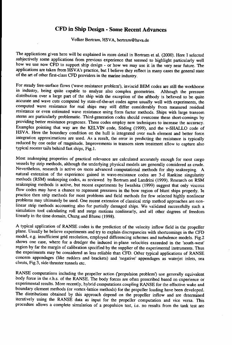
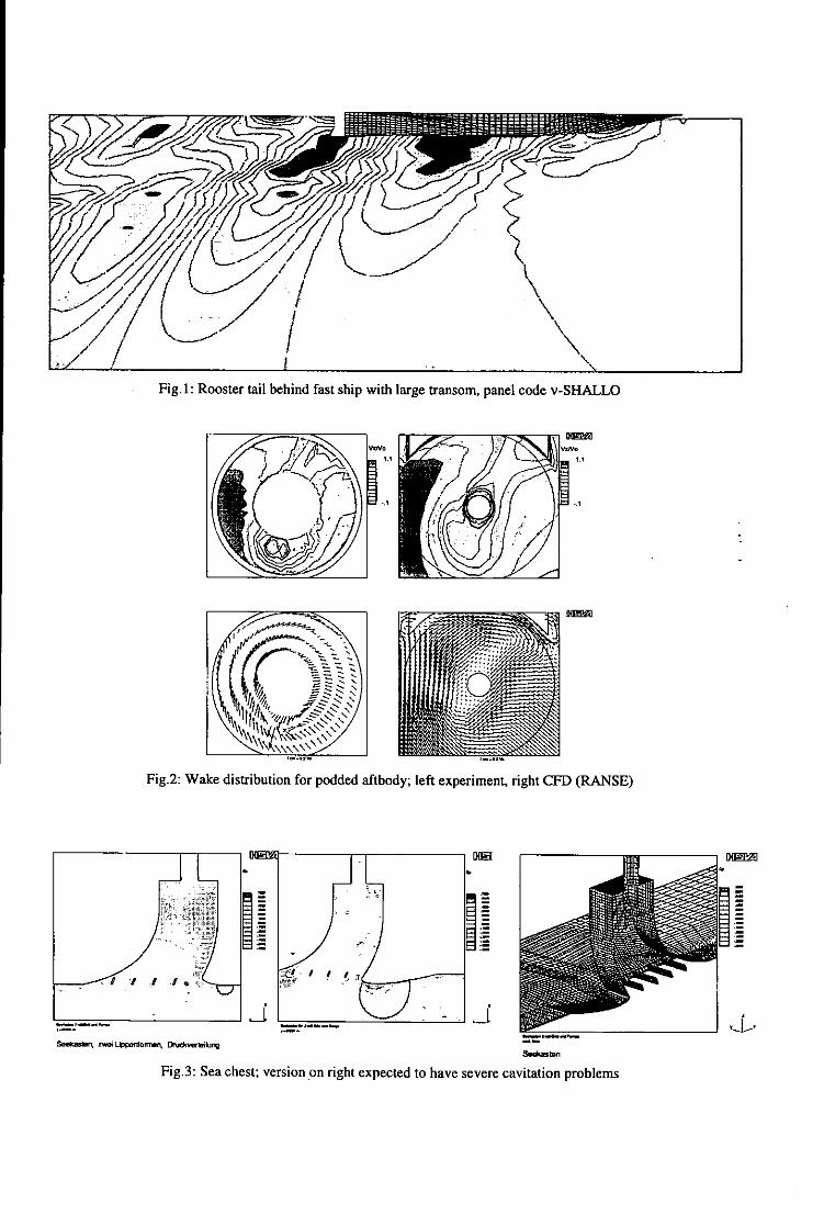
For steady free-surface flows ('wave resistance problem'), inviscid BEM codes are still the workhorsein industry, being quite capable to analyze also complex geometries. Although the pressuredistribution over a large part of the ship with the exception of the aftbody is believed to be quiteaccurate and wave cuts computed by state-of-the-art codes agree usually well with experiments, thecomputed wave resistance for real ships may still differ considerably from measured residualresistance or even estimated wave resistance using form factor methods. Ships with large transomstems are particularly problematic. Third-generation codes should overcome these short-comings byproviding better resistance prognoses. These codes employ new techniques to increase the accuracy.Examples pointing that way are the KELVIN code, S6ding (1999), and the v-SHALLO code ofHSVA. Here the boundary condition on the hull is integrated over each element and better forceintegration approximations are used. As a result, the error in predicting the resistance is typicallyreduced by one order of magnitude. Improvements in transom stem treatment allow to capture alsotypical rooster tails behind fast ships, Fig. 1.

Most seakeeping properties of practical relevance are calculated accurately enough for most cargovessels by strip methods, although the underlying physical models are generally considered as crude.Nevertheless, research is active on more advanced computational methods for ship seakeeping. Anatural extension of the experience gained in wave-resistance codes are 3-d Rankine singularitymethods (RSM) seakeeping codes, as reviewed by Bertram and Landrini (1999). Research on RSMseakeeping methods is active, but recent experiments by Iwashita (1999) suggest that only viscousflow codes may have a chance to represent pressures in the bow region of blunt ships properly. Inpractice then strip methods for most problems and field methods for few selected highly nonlinearproblems may ultimately be used. One recent extension of classical strip method approaches are non-linear strip methods accounting also for partially damaged ships. We validated successfully such asimulation tool calculating roll and surge motions nonlinearly, and all other degrees of freedomlinearly in the time domain, Chang and Blume (1998).

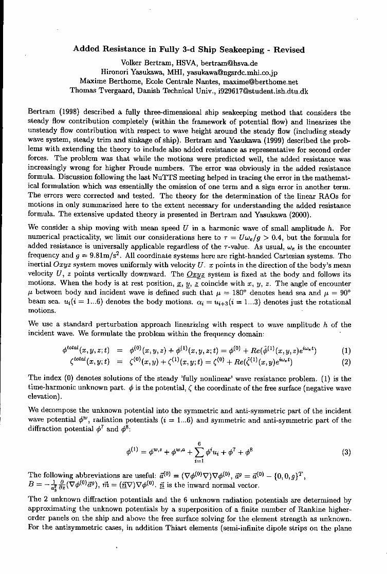
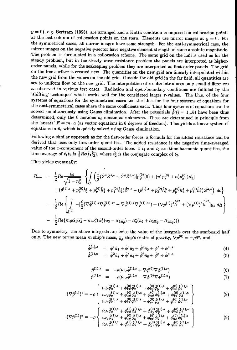
A typical application of RANSE codes is the prediction of the velocity inflow field in the propellerplane. Usually be believe experiments and try to explain discrepancies with shortcomings in the CFDmodel, e.g. insufficient grid resolution, employed differencing schemes and turbulence models. Fig.2shows one case, where for a dredger the induced in-plane velocities exceeded in the 'south-west'region by far the margin of calibration specified by the supplier of the experimental instruments. Thusthe experiments may be considered as less reliable than CFD. Other typical applications of RANSEconcern appendages (like rudders and brackets) and 'negative' appendages as waterjet inlets, seachests, Fig.3, side thruster tunnels etc.

RANSE computations including the propeller action ('propulsion problem') use generally equivalentbody force in the r.h.s. of the RANSE. The body forces are often prescribed based on experience orexperimental results. More recently, hybrid computations coupling RANSE for the effective wake andboundary element methods (or vortex-lattice methods) for the propeller loading have been developed.The distributions obtained by this approach depend on the propeller inflow and are determinediteratively using the RANSE data as input for the propeller computation and vice versa. Thisprocedure allows a complete simulation of a propulsion test, i.e. no results from the tank test are

required. Integral values like thrust deduction fraction t =(T-RT)/T, mean wake fraction w, propulsiveefficiency TID, hull efficiency 11H, and relative rotational efficiency "IR agree well with measurements.

The simultaneous consideration of viscosity and wave-making has progressed considerably over thepast decade. A number of methods try to capture wave making with various degrees of success. Mostreal ship flow problems require interface-capturing methods. Most schemes reproduce the waveprofile on the hull accurately, but problems persist with numerical damping of the ship wavepropagation, Fig.4. It is debatable if an accurate prediction of the wave pattern is necessary forpractical applications, but certainly everyone would prefer to see this problem overcome.

Predicting the flow around the hull and appendages (including propellers and rudders) in maneuveringis much more complicated than predicting the steady flow in resistance and propulsion problems.Often, both viscosity and free-surface effects play an important role. The rudder is most likely in thehull boundary layer, often operating at high angles of attack and in the propeller wake. The hull forcesthemselves are also difficult to predict computationally, because sway and yaw motions induceconsiderable cross flows with shedding of strong vortices. Most computations are also limited to smallyaw angles, with recent computations at HSVA for a ship at yaw angles up to 50' being a notableexception, Fig.5 and 6. The progress is promising, even though the time needed for such analyses isstill excessive for most practical applications.

Post-processing progresses as the core hydrodynamic analyses progress. State of the art are still staticviews. Series of snapshots are used for unsteady problems or complex geometries. Rarely and only forsimple geometries, we see animations for research applications. A natural extension to current post-processing may be Virtual Reality models, Barcellona and Bertram (2000). These allow a user to flythrough the model in space and time, with storage requirements one or two orders lower than forelectronic videos.

Acknowledgement

Many colleagues have supported this paper by supplying material from their respective experience.Foremost these are in alphabetical order Peter Blume, Andres Cura, Dieke Hafermann, JochenLaudan, Jochen Marzi, and Mathias Vogt.

References

BARCELLONA, M.; BERTRAM, V. (2000), Post-processing of time-dependent CFD analyses usingVirtual Reality Modelling Language, NuTTS'2000, Tjamo

BERTRAM, V.; CURA, A.; LAUDAN, J.; MARZI, J.; STRECKWALL; H. (2000), CFD simulationsin ship design, SIMOUEST, Nantes

BERTRAM, V.; LANDRINI, M. (1999), Panel methods for ship seakeeping computations, 31.WEGEMT School 'CFD for Ship and Offshore Design', Hamburg

CHANG, B.C.; BLUME, P (1998), Survivability of damaged ro-ro passenger vessels, ShipTechnology Research 45/3, pp. 105-117

IWASHITA, H. (1999), Prediction of diffraction waves of a blunt ship with forward speed takingaccount of the steady nonlinear wave field, NuTTS'99, Rome

SODING, H. (1999), Strdmungsberechnungen in der Schiffstechnik, Jahrbuch SchiffbautechnischeGesellscahft, Springer

24<

Fig. 1: Rooster tail behind fast ship with large transom, panel code v-SHALLO

•,o=

Fig.2: Wake distribution for podded aftbody; left experiment, right CFD (RANSE)

>w~

Scrt e

Fig.3: Sea chest; version on right expected to have severe cavitation problems

-5 / /

25 -- /

15 -A -?' C¾42 +" >X 1 7--crŽ

01 I IL I

30 - - - - - - - - - - - - - - - -15 5

I I I I I I I I25 .6 Sid foc cefcetfotakri ig.

Added Resistance in Fully 3-d Ship Seakeeping - Revised

Volker Bertram, HSVA, bertram@hsva.deHironori Yasukawa, MHI, yasukawa@ngsrdc.mhi.co.jp

Maxime Berthome, Ecole Centrale Nantes, maxime@berthome.netThomas Tvergaard, Danish Technical Univ., i929617@student.ish.dtu.dk

Bertram (1998) described a fully three-dimensional ship seakeeping method that considers thesteady flow contribution completely (within the framework of potential flow) and linearizes theunsteady flow contribution with respect to wave height around the steady flow (including steadywave system, steady trim and sinkage of ship). Bertram and Yasukawa (1999) described the prob-lems with extending the theory to include also added resistance as representative for second orderforces. The problem was that while the motions were predicted well, the added resistance wasincreasingly wrong for higher Froude numbers. The error was obviously in the added resistanceformula. Discussion following the last NuTTS meeting helped in tracing the error in the mathemat-ical formulation which was essentially the omission of one term and a sign error in another term.The errors were corrected and tested. The theory for the determination of the linear RAOs formotions in only summarized here to the extent necessary for understanding the added resistanceformula. The extensive updated theory is presented in Bertram and Yasukawa (2000).

We consider a ship moving with mean speed U in a harmonic wave of small amplitude h. Fornumerical practicality, we limit our considerations here to r = Uwe/g > 0.4, but the formula foradded resistance is universally applicable regardless of the T-value. As usual, we is the encounterfrequency and g = 9.81m/s 2 . All coordinate systems here are right-handed Cartesian systems. Theinertial Oxyz system moves uniformly with velocity U. x points in the direction of the body's meanvelocity U, z points vertically downward. The Oxyz system is fixed at the body and follows itsmotions. When the body is at rest position, x, y, z coincide with x, y, z. The angle of encounterit between body and incident wave is defined such that p = 1800 denotes head sea and p = 900beam sea. ui(i = 1...6) denotes the body motions. ai = ni+3 (i = 1...3) denotes just the rotationalmotions.

We use a standard perturbation approach linearizing with respect to wave amplitude h of theincident wave. We formulate the problem within the frequency domain:

ototal(xyz;t) = 4(o)(x,y,z) + ,(i)(x,y,z;t) = 4(O) + Re(6(1)(x,y,z)e i et) (1)ctotal(x, y; t) = ((O)(x, y) + c(i)(x, y; t) - (O) + Re(() (x, y)ewiet) (2)

The index (0) denotes solutions of the steady 'fully nonlinear' wave resistance problem. (1) is thetime-harmonic unknown part. € is the potential, ( the coordinate of the free surface (negative waveelevation).

We decompose the unknown potential into the symmetric and anti-symmetric part of the incidentwave potential e,1, radiation potentials (i = 1...6) and symmetric and anti-symmetric part of thediffraction potential 47 and 0s:

60(i) =k W'S + O + z + 07 + 48 (3)

The following abbreviations are useful: a- (° } - (V¢( 0)V)V4(°), 9 = 0(o) - {o, 0, g}T,B= --- a (v4( 0)M9), rfl (= V)V4,°). i is the inward normal vector.

The 2 unknown diffraction potentials and the 6 unknown radiation potentials are determined byapproximating the unknown potentials by a superposition of a finite number of Rankine higher-order panels on the ship and above the free surface solving for the element strength as unknown.For the antisymmetric cases, in addition Thiart elements (semi-infinite dipole strips on the plane

y = 0), e.g. Bertram (1998), are arranged and a Kutta condition is imposed on collocation pointsat the last column of collocation points on the stern. Elements use mirror images at y = 0. Forthe symmetrical cases, all mirror images have same strength. For the anti-symmetrical case, themirror images on the negative y-sector have negative element strength of same absolute magnitude.The problem is formulated in a collocation scheme. The same grid on the hull is used as for thesteady problem, but in the steady wave resistance problem the panels are interpreted as higher-order panels, while for the seakeeping problem they are interpreted as first-order panels. The gridon the free surface is created new. The quantities on the new grid are linearly interpolated withinthe new grid from the values on the old grid. Outside the old grid in the far field, all quantities areset to uniform flow on the new grid. The interpolation of results introduces only small differencesas observed in various test cases. Radiation and open-boundary conditions are fulfilled by the'shifting' technique' which works well for the considered larger r-values. The l.h.s. of the foursystems of equations for the symmetrical cases and the l.h.s. for the four systems of equations forthe anti-symmetrical cases share the same coefficients each. Thus four systems of equations can besolved simultaneously using Gauss elimination. After the potentials gi(i = 1...8) have been thusdetermined, only the 6 motions ui remain as unknowns. These are determined in principle fromthe 'ansatz' F = m . a (as vector equations in 6 degrees of freedom). This yields a linear system ofequations in fii which is quickly solved using Gauss elimination.

Following a similar approach as for the first-order forces, a formula for the added resistance can bederived that uses only first-order quantities. The added resistance is the negative time-averagedvalue of the x-component of the second-order force. If t, and t2 are time-harmonic quantities, thetime-average of t 1 t 2 is ½Re(4i t), where £ is the conjugate complex of .

This yields eventually:

R-Re - =• (2 +2fl ,* , ,,*(O) '(0)

R 1 + (2+ n2 Py )n 3

_•(p(1),s +_p(0) hs1 +y(O)h'a/• 4P(O)hs) 2 s ',* - (_0(1),a +p(xO)ha•p- +(O)hs +2_ p--(O)hia.,ga,*•.) c2 1- 2 z' 3z c+[e /p ý(') , +40 )/4 +pV)/4y2 aV+ (fi('t +p(Vfi4 +4 *h + p~y))a *) dS4

1 jf

26I- j-Re{mgd 1 &3 - inw2(&2(0 3 - &21g) - &3(r 2 + ±319 - &Iz))}

Due to symmetry, the above integrals are twice the value of the integrals over the starboard halfonly. The new terms mean m ship's mass, 1z, ship's center of gravity, Vp(°) = -pdg, and:

ý()s = Ifi,+ ý3 3 + ^ 55 + F7 + (4)

$()a 20'a + ý4f4+ $f60 + 0 + ýwQ (5)

=) --- p(iWe(1),S + VO (0 ),S) (6)

(1)_p(iw=(1),a + V(0)V(1),a) (7)

iUJN)S 04Ms + 0 + 4A4P$Z;iw 2, ~(0),s $ €.O.?(1),s '0_ .,,O)1),s •()(1),s"• )s (1),a +_ 0(h0) -£(I),a A(0) -(1)'a • (0)"•'(1)'x y Y 0 , a I (8)

+(1),S + A(),)s +40•4(0)• ()(),s{ Wz tz w ' + X (( , y +z -) - z )+•'),a +_ 4.() ( ,),s a- ()(0 ) -. Y ,s +_ 0x(°). ),a 9

(V OM( )). _P • - '::y S' -0) -M S ' (0) -M S ' (0)-M

• • ( 1 ) , a • ( 0 ) , - ( 1 ) ,a 0 ) . -/ O ) ( 1 ) ,a ,/ ( 0 ) -• ( ' ) ,a•lwJ z + 01Z 01 , + 4z q5y ", +zz 0z

-. =dxi+u h +h = 6X__6-Yý4z+,f2 + O (10)

+'s2: + i3 ( 4Y_

a+ - fi3 + "i5x_ = a has

a3 3a2a zw iwe(1) 'a +r v&Ov(°)V• 1 a + 1• (-

1)__ -

a] 4 a~y_ =pag

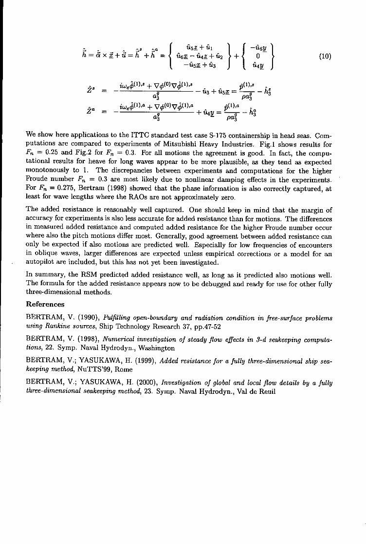
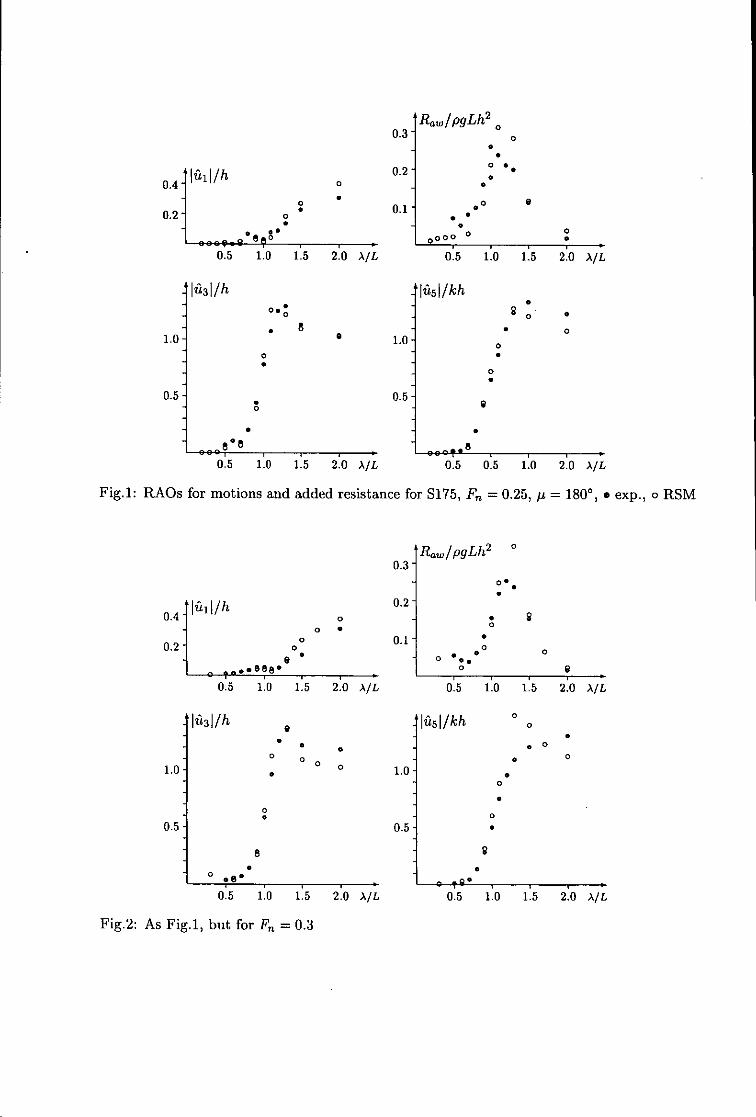
We show here applications to the ITTC standard test case S-175 containership in head seas. Com-putations are compared to experiments of Mitsubishi Heavy Industries. Fig.1 shows results forFn = 0.25 and Fig.2 for F. = 0.3. For all motions the agreement is good. In fact, the compu-tational results for heave for long waves appear to be more plausible, as they tend as expectedmonotonously to 1. The discrepancies between experiments and computations for the higherFroude number F. = 0.3 are most likely due to nonlinear damping effects in the experiments.For F. = 0.275, Bertram (1998) showed that the phase information is also correctly captured, atleast for wave lengths where the RAOs are not approximately zero.

The added resistance is reasonably well captured. One should keep in mind that the margin ofaccuracy for experiments is also less accurate for added resistance than for motions. The differencesin measured added resistance and computed added resistance for the higher Froude number occurwhere also the pitch motions differ most. Generally, good agreement between added resistance canonly be expected if also motions are predicted well. Especially for low frequencies of encountersin oblique waves, larger differences are expected unless empirical corrections or a model for anautopilot axe included, but this has not yet been investigated.

In summary, the RSM predicted added resistance well, as long as it predicted also motions well.The formula for the added resistance appears now to be debugged and ready for use for other fullythree-dimensional methods.

References

BERTRAM, V. (1990), Fufilling open-boundary and radiation condition in free-surface problemsusing Rankine sources, Ship Technology Research 37, pp.4 7-5 2

BERTRAM, V. (1998), Numerical investigation of steady flow effects in 3-d seakeeping computa-tions, 22. Symp. Naval Hydrodyn., Washington

BERTRAM, V.; YASUKAWA, H. (1999), Added resistance for a fully three-dimensional ship sea-keeping method, NuTTS'99, Rome

BERTRAM, V.; YASUKAWA, H. (2000), Investigation of global and local flow details by a fullythree-dimensional seakeeping method, 23. Symp. Naval Hydrodyn., Val de Reuil

Ran/pgLh 2 00.3- o

o.

I 0.2"

0.2-o 0o .o

-. 0_ •0000

0

0.5 1.0 1.5 2.0 AlL 0.5 1.0 1.5 2.0 A/L

lai~llh lasll/kh

20 0

1.0 00

00

0.5 0.50*

0.5 1.0 1.5 2.0 A/L 0.5 0.5 1.0 2.0 AIL

Fig. 1: RAOs for motions and added resistance for S175, Fn = 0.25, p = 1800, * exp., o RSM

Raw/pgLh 2 0

0.3-

J4 tIall/h 0.2-00

0 0

0 * 0 0

0

0.5 1.0 1.5 2.0 A/L 0.5 1.0 1.5 2.0 A/L

1f3l/h l 1t51/kh 0

C .00 0 0

1.0 . o 1.00

0* 0

0.5 0.5-

0 *.oCo

0.5 1.0 1.5 2.0 A/L 0.5 1.0 1.5 2.0 A/L

Fig.2: As Fig.1, but for F. = 0.3

Numerical Simulation of Planing HullsMario Caponnetto, Rolla SP Propellers SA, Switzerland, mario.caponetto@rolla-propellers.ch

The present paper deals with the numerical simulation of the flow on hard chine planing vessels. In the past it has beendifficult to study this kind of vessel by means of the available methods, such as panel methods, usually applied toconventional ships. The reason is due to the particularly complicated flow field generated by planing hulls.A thin layer of water (spray) is generated at the stagnation line, and in this zone the pressure gradient is very high.Depending on the hull shape and speed the flow may separate sharply at the chine, and eventually reattach along thehull sides, or generate vortices. The transom can be dry at high speed, while partly wetted, with recirculating water, atlower speed. The generated bow and stern waves are normally steep and may break, dissipating their content of energy.Due to these particular features, potential flow methods are not suitable for planing hull computation, nor are anymethods that are unable to compute highly geometrically nonlinear free surfaces.The method presented in this paper approaches the problem using a RAP/S code based on Finite Volumes, where thefree surface is computed using a Front-capturing Method (Volume of Fluids).The results obtained using this method for real hull shapes and monoedric hulls are very satisfactory; some examplesare presented in the paper.

Introduction

Hard chine planing hulls represent nearly the totality of the vessels employed in the nautical field for pleasure crafts,and are also largely used for small and medium size civil and military applications.Despite this fact there is a lack of tools at disposal of the naval architect to design, analise and optimize this kind ofvessel. The analytical method normally used to predict the resistance and the trim of the boat is the well known Savitskymethod, with its variations. The main drawback is that the Savitsky method is strictly applicable only for monoe-drichull shapes, namely any variation of the beam and deadrise angle cannot be properly taken into account. The formulaare a mixture of experimental and theoretical data and some of the approximations adopted may become important. Forexample the effect of the hydrostatic pressure and the position of the center of pressure are a too simple approximationof the real phenomenon. In general large errors may occur for warped hulls and when computing performances at lowspeed.There are also a number of systematic series, but again the shape of the real planing hulls used nowadays normallydiffers from that of the series.Moreover it is not a common practice of the majority of the shipyards to perform model testing in the towing tank, andthis is mainly due to the obvious time and cost constraints typical of small boats.All these factors make the prediction of planing boat performance more an art then a science, and the result is a largemargin of uncertainty.The need for a reliable direct method able to compute the flow field around planing hulls is then highly requested bydesigners, but the mathematical complications due to the complexity of the flow are obvious. This is due to the presenceof the spray, detachment of the flow at the chine and reattachment along the side, complicated flow at the transom andpresence of breaking waves.A number of recently developed CED codes are now able to compute flows with large deformations of the free surface.Particularly successful are those adopting the Volume of Fluid technique. In this case both air and water are computedsimultaneously; the two fluids are not considered separately, but as a continuum fluid with different physical properties.The physical property of the actual fluid depends on the properties of the two constituent fluids and a scalar quantity (C)that represents the volume fraction of the two phases (i.e. C= I for water and C=O for air). A value of C between 0 and Iindicates the presence of the interface, that is not discontinuous but mainly depending on the mesh size.A similar approach is used in the commercial code Comet, developed at the ICCM of Hamburg. The code is a FiniteVolume method able to solve RANS equations with the additional above mentioned capability to include free surfacecalculation.The code has been used to compute a large number of planing hulls and the comparison with the available experimentaldata has been very satisfactory. Accurate resistance curves for different displacements and center of gravity positionscan now be computed in a couple of days, with obvious advantages for the boat (and propeller) designers.

Mesh and test procedure

An accurate and efficient mesh is needed to compute the flow field with the requested precision and within practicaltime constraints. While Comet allows both structured and unstructured mesh, for our problem we use multi-block meshwith structured hexahedral cells. Nine blocks are normally used to define the computational domain, distributing thecells between the blocks in order to refine the mesh where the gradients are expected to be higher. Cells are refinedalong the hull surface to capture the spray and the boundary layer, as well as above and below the undisturbed watersurface to compute waves. Cells do not have to match at block interfaces. A typical mesh is represented in figure 1.

0

0 fl 2

14

16

120

Figure I

After a number of convergence tests we have noticed that, while the flow detail increases with the cell number, a meshhaving about 400.000 cells (for one half of the boat) is sufficient to have converged values of the forces acting on thehull (lift and drag) and of the center of pressure.Given the hull shape, displacement, center of gravity and speed, the trim of the boat remains unknown. In theory weshould test different trim (and submergence) until we obtain, with a trial and error procedure, the trim that satisfies theequilibrium of the forces and moments. Since the displacement of the boat may vary and moreover we could beinterested to know how the resistance changes moving the center of gravity, we prefer to test the boat at a number ofpredefined trim and submergence, to compute the lift, resistance and the center of pressure, and then to interpolate thesevalues at the desired displacement (lift) and center of gravity (center of pressure).In general for each speed the boat is tested at a combination of 3 trim angles and 3 immersions of the transom. Theresults of the 9 tests allow later a bi-quadratic interpolation of the values. While Comet can perform parallelcomputation, in our case it is has been found convenient to run the cases serially, each one on a different processor thatwe have at disposal (2 processors of SGI Octane, 4 processors of SOT Origin 2000).Figures 2 and 3 show some typical result; in this case the data are for a 80 foot boat at 34 knots. Figure 2 shows how theposition of the center of pressure (from transom) and the lift change with trim and submergence. Each curve is for adifferent trim angle (2, 3 and 4 degrees), while each point over the curve is a different submergence at the transom.Figure 3 shows similar results for the total resistance.In many cases not only the value of the forces are of interest, but also the pressure distribution and the wave patternvisualization can be useful to understand the behavior of the boat. Figure 4 shows the free surface elevation calculatedfor a boat with unusual hull shape running at 40 knots. It can be observed the rise of the spray at the stagnation line; thespray is then deflected at the chine and moves sideway generating a thin breaking wave. The level of the free surface istaken conventionally where the volume fraction is C=0.5.

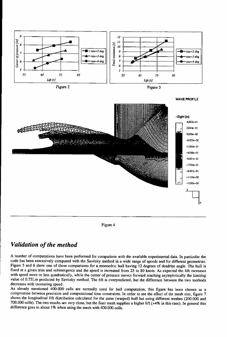
9 12 ,

6 '-.11~~8 _______ - 10 ____

U-- tau=2 deg 9 -U-tau=2 degL7

_ S 8 -----&--iau=3 deg = - a3 deg6 _____ "-'-u=4 deg Z 7 --- tau=4deg

5 __6 [5 •

55 65 75 85 55 65 75 85

Lift Id Lift Id

Figure 2 Figure 3

WAVE PROFILE

-Eight [m)

4.357e-0J1

2.634e-019,0(C•e-02

-8.323e-02

-2.565e-01

-4298e-01

-6.031 e-01

-7764e-01

-9.497e-01

-1.123e.00

-1.296e+00

Y

Figure 4

Validation of the method

A number of computations have been performed for comparison with the available experimental data. In particular thecode has been extensively compared with the Savitsky method in a wide range of speeds and for different geometries.Figure 5 and 6 show one of these comparisons for a monoedric hull having 12 degrees of deadrise angle. The hull isfixed at a given trim and submergence and the speed is increased from 25 to 80 knots. As expected the lift increaseswith speed more or less quadratically, while the center of pressure moves forward reaching asymptotically the limitingvalue of 0.75Lm predicted by Savitsky method. The lift is overpredicted, but the difference between the two methodsdecreases with increasing speed.As already mentioned 400.000 cells are normally used for hull computation; this figure has been chosen as acompromise between precision and computational time constraints. In order to see the effect of the mesh size, figure 7shows the longitudinal lift distribution calculated for the same (warped) hull but using different meshes (200.000 and700.000 cells). The two results are very close, but the finer mesh supplies a higher lift (+4% in this case). In general thisdifference goes to about 1% when using the mesh with 400.000 cells.

16W 9

12W 7___

1,0 P____40 ý.

0 0 __

0 X0 40 60 W0 0 20 M/ M0 8

Figure 5 Figure 6

30000 - __ ___

25000 - _ _

20000 - -s- 200000 cells150 -___ ___-- 700000 cells

S10000 - ____ S_ _ __ B Stat. press.

5000 -___J

0 5 10 15 20 25

X [m]

Figure 7

Figure 7 shows that the lift increases steeply from the point of attachment of flow at the keel (X=8 m) to the point ofdetachment at the chine (X=15 in). Then the lift decreases, going rapidly to zero close to the stemn, since in this case thetransom was completely dry.

Conclusion

In this paper has shown the possibility to compute planing hull flow using a numerical method. The method used isbased on the Finite Volume formulation and the free surface deformation is computed using a Volume of Fluidapproach. With this technique it is possible to predict the complex behavior of the flow typical of planing hulls (spraygeneration, detachment and reattachment of the water at the chine, breaking waves). The computed forces are in generalin good agreement with the experimental data available, and some comparison is presented in the paper. Any realistichull shape can be computed, and this is a great improvement for planing hull designers, compared with the methodscommonly used in the past.

An Investigation of the Time-Step for a Line-Implicit Time-Stepping Schemefor the k - w and Reynolds-Averaged Incompressible Navier-Stokes Equations

Lars CarlssonHydromechanics division

Department of Naval Architecture and Ocean EngineeringChalmers University of Technology

SE-412 96 Gdteborglc@na.chalmers.se

Extended Abstract

This is work in progress. Eventually we want to compute turbulence modeled unsteadyflow in boundary layers. More specifically, the flow around sails and hulls. We will advancethe solution in time using a second-order accurate method and we want to avoid the severetime-step restrictions that occur in boundary layers for explicit methods. If our investigationturns out well and time permits, we will add the time-stepping algorithm to an existing flowsolver and present some computations.

We will investigate the impact of a line-implicit time-stepping technique on the size ofthe time-step in a turbulence modeled channel flow. The turbulence model that we are goingto investigate is a k - w-model along with a velocity-pressure formulation of the Reynolds-averaged incompressible Navier-Stokes equations. Previous results, for the incompressibleNavier-Stokes equations, show that it is possible to split the spatial operators in the momen-tum equations and treat components belonging to a specific grid direction implicitly and therest of the terms explicitly.

The flow solver is based on a discretization in space on what is known as Chimera orcomposite overlapping grids. This discretization technique gives us the possibility to choosethe type of time-stepping scheme to be used in each component grid individually. Anotherbenefit is that the Chimera technique also lets us construct body-fitted grids that resolveboundary layers. At each time step we want our flow solver to accurately predict the lengthof the largest possible time step. The algorithm for the time-step prediction rely on vonNeumann analysis of the amplification factors. The von Neumann analysis in turn is onlyvalid for periodic solutions. Instead a more computationally costly technique could be used;computing the amplification factors for a semi-discrete case. In practice this is not an option,because in addition to solving the governing equations, we would have to solve a correspondinggeneralized eigenvalue problem.

Our analysis will be conducted for a two-dimensional channel with periodic boundaryconditions in the x-direction and no-slip boundary conditions in the y-direction. Within thisinvestigation, we hope to find answers to two questions; Can the operators in the k - w-modelequations be divided to accomplish a stable time-stepping algorithm using a large time step?How does the amplification factors estimated by the von Neumann analysis correspond tothose in the channel case?

Study on the Hydrodynamic Characteristics ofFoil-Assistance Arrangement for a Catamaran

S. W CHA U C. C. JAN C.L H WANGUnited Ship Design and Development Center Institute of Naval Architecture and Ocean

TAIWAN, R.O.C Engineering, National Taiwan UniversityTAIWAN, R.O.C.

1. INTORDUCTION for designing the foil-assistance system of catamarans.

Recently the United Ship Design and Development 2. EXPERIMENTAL STUDYcenter (USDDC) has devoted efforts to develop high- A 25mn long passenger catamaran with foil-assistancespeed catamarans for passenger transport. Foil-assistance arrangement, Fig. 1, has been tested in the large towingarrangement is employed to increase the service speed tank at the Institute of Naval Architecture and Oceanand improve the ride performance. Two demi-hulls of Engineering of National Taiwan University [1]. The foilcatamaran can provide good support and protection for system is comprised of two hydrofoils. The main foilhydrofoils, and hence they generally extend between the located near LCB provides lift to reduce total resistance,demni-hulls. The main advantage of hydrofoil is the low and the sub-foil near stem gives pitching moment tocost of installment, and high effectiveness in speed improve riding performance. Both foils are tested at 00,increase. Hydrofoils are often installed with fixed 20 and 50, respectively. Two different longitudinalorientation on ship. This leads to that the cost for building positions for aft foil are used to study the influence onand maintaining is relatively low. The speed increase total resistance due to the sub-foil. The ship with bothmainly depends on the section shape of hydrofoil, the foils installed are tested from Fn=0O. I to 1.2. Additionally,longitudinal position, the vertical position, and the angle the catamaran only with main foil installed is also tested.between foil and hull. From the resistance point of view, This can help to simplify the hydrofoil flow field andthe lift-drag ratio of hydrofoil is especially important. analyze the catamaran-foil system more easily, becauseThe hydrodynamic lift generated by hydrofoils can there is strong interaction between two hydrofoils. Ourreduce the displacement of ship, and hence also the total numerical computation only focuses on the last case. Theresistance. However, the hydrodynamic drag compensates force measurement device is specially designed that thethe resistance decrease effect. Generally speaking, the hydrodynamic lift and drag of the hydrofoil can berequired propulsion power can be obviously reduced at precisely and separately measured [I].high Froude number, but could be little influenced for 3. SIMPLIFIED NUMERICAL COMPUTATIONlow Froude number. Due to the small draft of catamaranthe hydrofoil should have its submergence as deep as The numerical model of the interested case is simplifiedpossible to reduce the free surface effect, because it due to the following two main reasons: First, thecauses considerably loss of hydrodynamic lift. The complete three-dimensional computation of thelongitudinal position of hydrofoil can help catamaran to catamaran with hydrofoil is too time-consuming andkeep a favorable trim and minimum resistance. Because complicated, which is not very practical in the designthe trim angle of catamaran is small, a sufficient large stage. Second, an engineering approach based onangle of attack for hydrofoil is necessary to provide simplified theories and experimental correlations is morerequired lift. Too large angel of attack is not preferred due preferable for design purpose. Although the flow aroundto its rapid drag increase. foil is three-dimensional, it seems to approach two-The flow around hydrofoil is basically three- dimensional at high Froude. The wave system induced by

dimensional, although it is hounded by two demi-hulls. two demi-hulls is also neglected for the sake ofBesides, the wave system generated by the interaction of simplicity. Ship performance is interested at the designtwo demti-hulls make the hydrofoil flow more speed (high Froude number) in the design stage, whichcomplicated. The foil-assistance system has been seems to justify the two-dimensional and no hullinvestigated using experimental approach discussed in the assumption. But the angle of attack of hydrofoil withnext section. This paper tries to isolate the hydrodynamic respect to the still water line and the submergence of foilbehavior of hydrofoil from the complete system by using are directly taken form the experimental data.measured results and a simplified numerical computation Extensive study of two-dimensional hydrofoils withoutin order to understand the hydrodynamic characteristics considering the free surface effect is performed by Chau

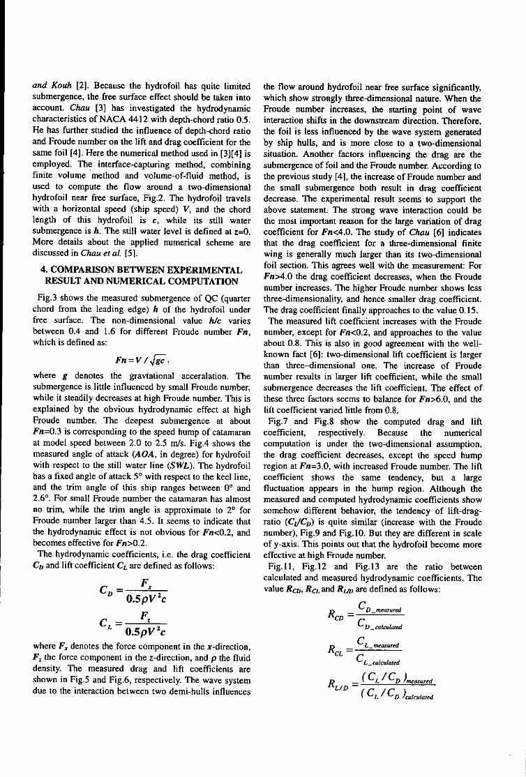
and Kouh [2]. Because the hydrofoil has quite limited the flow around hydrofoil near free surface significantly,submergence, the free surface effect should be taken into which show strongly three-dimensional nature. When theaccount. Chau [3] has investigated the hydrodynamic Froude number increases, the starting point of wavecharacteristics of NACA 4412 with depth-chord ratio 0.5. interaction shifts in the downstream direction. Therefore,He has further studied the influence of depth-chord ratio the foil is less influenced by the wave system generatedand Froude number on the lift and drag coefficient for the by ship hulls, and is more close to a two-dimensionalsame foil [4]. Here the numerical method used in [3][4] is situation. Another factors influencing the drag are theemployed. The interface-capturing method, combining submergence of foil and the Froude number. According tofinite volume method and volume-of-fluid method, is the previous study [4], the increase of Froude number andused to compute the flow around a two-dimensional the small submergence both result in drag coefficienthydrofoil near free surface, Fig.2. The hydrofoil travels decrease. The experimental result seems to support thewith a horizontal speed (ship speed) V, and the chord above statement. The strong wave interaction could belength of this hydrofoil is c, while its still water the most important reason for the large variation of dragsubmergence is h. The still water level is defined at z--0. coefficient for Fn<4.0. The study of Chau [6] indicatesMore details about the applied numerical scheme are that the drag coefficient for a three-dimensional finitediscussed in Chau et al [5]. wing is generally much larger than its two-dimensional

4. COMPARISON BETWEEN EXPERIMENTAL foil section. This agrees well with the measurement: ForRESULT AND NUMERICAL COMPUTATION Fn>4.0 the drag coefficient decreases, when the Froude

number increases. The higher Froude number shows lessFig.3 shows the measured submergence of QC (quarter three-dimensionality, and hence smaller drag coefficient.

chord from the leading edge) h of the hydrofoil under The drag coefficient finally approaches to the value 0.15.free surface. The non-dimensional value h/c varies The measured lift coefficient increases with the Froudebetween 0.4 and 1.6 for different Froude number Fn, number, except for Fn<0.2, and approaches to the valuewhich is defined as: about 0.8. This is also in good agreement with the well-

known fact [6]: two-dimensional lift coefficient is largern = V / rgthan three-dimensional one. The increase of Froude

where g denotes the gravtational acceralation. The number results in larger lift coefficient, while the smallsubmergence is little influenced by small Froude number, submergence decreases the lift coefficient. The effect ofwhile it steadily decreases at high Froude number. This is these three factors seems to balance for Fn>6.0, and theexplained by the obvious hydrodynamic effect at high lift coefficient varied little from 0.8.Froude number. The deepest submergence at about Fig.7 and Fig.8 show the computed drag and liftFn=0.3 is corresponding to the speed hump of catamaran coefficient, respectively. Because the numericalat model speed between 2.0 to 2.5 m/s. Fig.4 shows the computation is under the two-dimensional assumption,measured angle of attack (AOA, in degree) for hydrofoil the drag coefficient decreases, except the speed humpwith respect to the still water line (SWL). The hydrofoil region at Fn=3.0, with increased Froude number. The lifthas a fixed angle of attack 50 with respect to the keel line, coefficient shows the same tendency, but a largeand the trim angle of this ship ranges between 00 and fluctuation appears in the hump region. Although the2.60. For small Froude number the catamaran has almost measured and computed hydrodynamic coefficients showno trim, while the trim angle is approximate to 2' for somehow different behavior, the tendency of lift-drag-Froude number larger than 4.5. It seems to indicate that ratio (C,/CD) is quite similar (increase with the Froudethe hydrodynamic effect is not obvious for Fn<0.2, and number), Fig.9 and Fig.10. But they are different in scalebecomes effective for Fn>0.2. of y-axis. This points out that the hydrofoil become moreThe hydrodynamic coefficients, i.e. the drag coefficient effective at high Froude number.

CD and lift coefficient CL are defined as follows: Fig.l1, Fig.12 and Fig.13 are the ratio betweencalculated and measured hydrodynamic coefficients. The

CD = F, value RcD, RCL and R1u, are defined as follows:0.5 p V 2 c C

CL= F_ Rc= -D mesrd0.5pV 2c CD-catcU•aedCmeasured

where F., denotes the force component in the x-direction, R L -F, the force component in the z-direction, and p the fluid CL-calculaed

density. The measured drag and lift coefficients areshown in Fig.5 and Fig.6, respectively. The wave system RL - (CL/CD )easureddue to the interaction between two demi-hulls influences (C/C )acula.d

The Rcv value is about 4.2 for Froude number larger than4.0. This means that the calculated value from thesimplified assumption is too small. But it is a good wayto estimate the three-dimensional drag coefficient in theprimary design stage. The RCL value deviates from 1.0 forsmall Froude number, but it is quite close to 1.0 at designspeed. This indicates that the two-dimensionalassumption is acceptable for very high Froude number(>8.0). To estimate the Rtm value from the numericalcomputation, the measured one is only about 25% of thecalculated one due to too small drag prediction innumerical computation.

5. CONCLUSION

The prediction of the hydrodynamic coefficients for asingle hydrofoil installed on a 25m long passengercatamaran has been performed both numerically andexperimentally. The numerical computation is performedunder the two-dimensional flow assumption andneglecting the interaction between hull and foil. At highFroude number the measured lift coefficient of hydrofoilapproximates the value for two-dimensional case, and thedrag coefficient for two-dimensional one is about 25% ofthe experimental result.

REFERENCES

1. Model Test for a High-Speed Catamaran, United ShipDevelopment Center (1999).

2. Chau, S.W., Kouh, J.S., "Analysis of IncompressibleFlow around Profiles Used for Marine Applications",Bulletin of the College of Engineering, N.T.U., No.76,pp 8 5 -10 2 (1999).

3. Chau, S.W., "On the Hydrodynamic Performance of a2D-Foil near Free Surface", Proceeding of the SeventhNational Conference on Naval Ship Engineering,pp.21-28 (1999).

4. Chau, S.W., "Numerical Study of Small SubmergedDepth on Hydrodynamic Coefficients of a Two-Dimensional Hydrofoil at High Froude Number",Proceedings of the Sixth National Conference onComputational Fluid Dynamics, pp.656-661 (1999).

5. Chau, S.W., Peric, M., Muzaferija, S., "An Interface-Capturing Method for Prediction of SloshingProblems", Proceedings of the 22nd NationalConference on Theoretical and Applied Mechanics,Vol.2, pp.363-370 (1998).

6. Chau, S.W., "Numerical Investigation of Free-StreamRudder Characteristics Using a Multi-Block FiniteVolume Method", Bericht Nr. 580, IfS der Uni.Hamburg (1997).

4A -- ---- '-• ---. -• .. ..---I I if lCII I I I

40I I I I

I I IFig.l (left) A 25m long passenger catamaran with s.o ... .. - ---- , . ---Uhydrofoil arrangement I 1 ,

Fig.2 (right) Schematic sketch of hydrofoil near free I a?-o - T - --" ', --- i --L, -surface,,

S- 1.0. . ... . .. . . . . .. .. . --- - -- -- - - -- - -- - -- -- -- - --TT----------........ .... --

...... I

---- ----- .------ 0--- 0.0 2.0 A am 8a0 10.0

Fig ....--- _ -. i"K Fig. 11 RcD value of hydrofoil at different Fna~~lG N.. . . . . . . . . . A .. . I

Fig.3 (left) Submerged depth of hydrofoil under freesurface 1.2 ----- ..----------------

Fig.4 (right) Angle of attack for hydrofoil with respectto SWL .o- --........--- .- ------

tab 0.8

~~o..... ....... r..... ............--.- --- ----...--.------- - - 0.4-- -- .. -- ------ -----------

Fi 5fl0.2 . . . . . . . . .n5(left) Measured Cd of hydrofoil at different F-

Fig.6 (right) Measured CL. of hydrofoil at different En

.... ............. Fig.12 RcL. value of hydrofoil at different Fnt---.--------------------- -----------------

-ig - ........ Ii--i--ti-....... .

cr i sa cFig.7 (left) Computed CD of hydrofoil at different Fn 0.• " 4......... .... .0Fig.8 (right) Computed CL of hydrofoil at different Fni

0.2 ------------ ........----------------

[1 3A ---------- 1----

I I 2 L0.0 ----------

c . ... (lelJ) C. Fig. 13 Rh o value of hydrofoil at different Fn

Fig.9 (lf)Measured LID value of hydrofoil atdifferent Fn

Fig.0 (right) Computed CL/ value of hydrofoil at

different Fnt

Comparison of Explicit Algebraic Stress Models and Second-OrderTurbulence Closures for Steady Flows around the KVLCC2 ship at

model and full scales

G.B. Deng & M. VisonneauLaboratoire de M6canique des Fluides, Ecole Centrale de Nantes

1 Rue de la Nod, B.P. 92101, 44321 Nantes Cedex 3, FranceFax: (33) 2 40 37 25 23

E-Mail: Ganbo.Deng@ec-nantes.fr, Michel.Visonneau@ec-nantes.fr

June 30, 2000

1 IntroductionThis paper is devoted to the assessment of the most recent turbulence models for steady flows around amodern ship, the so-called KVLCC2 ship which has been studied experimentally by Dr. Kim & al. atKRISO [8]. The flow is characterized by a strong thickening of the boundary layer, the generation of anintense longitudinal vortex motion creating complex "hook-shaped" velocity contours in the central part ofthe wake near the location of propeller.

The aim of this study is therefore, (i) to compare, at model scale, the relative merits of different statisticalclosures ranging from eddy-viscosity models to second-order formulations based on the Reynolds Stresstransport equations, (ii) to evaluate, at full scale, the differences between the solutions provided by thevarious models in order to check if the dependancy of the solution on the turbulence modelisation is alsocritical for flows around real ships.

2 Numerical MethodThe simulation has been performed with the HORUS code developed in our CFD group (Division Mod6lisationNum6rique). The solution of the Reynolds Averaged Navier-Stokes Equations is obtained by using finite dif-ference method with a body-fitted structured grid. A cell-centered layout is employed in which the pressure,turbulence and velocity unknowns share the same location. The momentum and continuity equations arecoupled through the PISO procedure and several implicit first and second order accurate schemes are im-plemented for the space and time discretizations. In the present computation, convection terms written inconvective form are discretized with a third order upwind-biased scheme which is similar to the well knownQuick scheme for the conservative formulation. Finally, preconditioned conjugate gradient solvers (CGS,CGSTAB) are used to solve the linear systems.

Implementation of Reynolds stress transport model in a non-staggered layout is not straightforward. Dueto the absence of numerically stabilizing eddy viscosity and the predominant influence in the momentumtransport equations of the equilibrium between several strong and opposite source terms, namely the pressureand Reynolds stress gradients, a special numerical stabilizing technique has to be implemented. The maincharacteristics of these numerical amendments are recalled in previous contributions of Deng & Visonneau([3], [2]).

2.1 Reynolds Stress ModelsThe Rij-w closure which has been used in this study is a more robust variant of the original Shima model[9] which shares the same overall formulation but differs only in the model coefficients. The Reynolds stresstransport equations are not recalled here for the sake of brevity here but can be found in [3].

2.2 Explicit Algebraic Stress ModelBy using a local equilibrium assumption, Rodi [7] has deduced an algebraic stress model (ASM) from theReynolds stress transport model. Actually, the ASM model can be explicitly solved and such an explicitalgebraic stress model (EASM) has been first proposed by Pope [6] for two-dimensional flows. EASM modelsfor three-dimensional flows have been developed by Gatski & Speziale [4] and are widely used. In thisstudy, we use the EASM model proposed by Gatski & Speziale [4] based on a three-term basis which is theexact solution of the ASM model only for 2D flows. For three-dimensional flows, this formulation can beonly considered as an approximation. However, it is expected that this model can improve the predictioncompared with a linear eddy-viscosity model. Here again, the details of the closure modified by the authorsin the near-wall region are not recalled here but can be found in [3].

3 Numerical Results

Computations have been performed on a domain covering the whole ship with 121 x 81 x 41 nodes in thestreamwise, radial and girthwise directions respectively. A third order upwind-biased scheme is used todiscretize the convection term. The convergence is ensured by checking the evolution of the wall frictionvelocity. Several thousand iterations are necessary to achieve convergence. Computational time with theReynolds stress model is about twice more important than with the EASM or two-equation models.

X/L=0.485 is the station where the propeller should be present. The successful prediction of the hook-shaped mean streamwise velocity contours observed in the measurements has always been considered as akey criterion for assessing the performance of a turbulence model designed for ship flows.

By comparing the predicted mean streasnwise velocity contours with the experimental measurements atthis station (figures l(a) to 1(c)), it can be observed that the hook-shaped velocity contours are remark-ably well captured with this new Reynolds stress model (figure 1(c)). However, an additional secondaryvortex near the vertical plane of symmetry is found by the second order model, which is not present inthe experiments. With the EASM model and the SST model, the streamwise velocity at the center of thelongitudinal vortex is clearly under-predicted. The EASM-SSG model provides a simulated flow in slightlybetter agreement with the experiments (figure l(b)) but the improvement is not spectacular.

Figures 2(a) to 2(b) show the predicted turbulent kinetic energy scales obtained with a K - w and theRij - w models. All the models implemented tend to overpredict the maximum value of the turbulent kineticenergy near the plane of symmetry. However, the prediction provided by the Rij - w model is the closestfrom the experiments.

In a previous study on the HSVA tanker, Deng & Visonneau [3] found that the sum of the convectionand the turbulent diffusion terms in the turbulent kinetic energy budget was almost as important as theturbulent dissipation term in this region. Consequently, the convection and the turbulent diffusion terms,intrinsically present in the Reynolds stress transport equations, should not be neglected. This analysis hasnot yet been done for this testcase but all the results available here suggest that this explanation is also validfor this ship.

Finally, the computations are performed at the full scale Reynolds number. It is very encouraging tosee that no particular numerical problems appear during these validations. Figures 3(a) to 3(b) show theisowakes and turbulent kinetic energy contours simulated by the K - w and the Rij - w closures. First,compared with the model scale, the overall intensity of the longitudinal vorticity is drastically reduced sincethe convection effect is more important. However, the importance of the turbulence modelisation is stillclearly illustrated by these results since the second-order closure provides again a significantly more intenselongitudinal vorticity.

2

4 Concluding RemarksThe flow around the KVLCC2 ship has been calculated by using different turbulent models ranging fromlinear eddy-viscosity model, explicit algebraic stress model, to full Reynolds stress transport model. A stablesolution of the Reynolds stress transport equations has been obtained by implementing the same near-wallmodel and defect correction approach already validated on the HSVA tanker (Deng & Visonneau, [3]).

On one hand, non-linear models obtained from an approximate explicit solution of the algebraic stressmodels slightly improve the prediction in all aspects compared with simple linear eddy-viscosity models.However, the solution of the Reynolds stress transport equations shows that the local equilibrium assumptionon which the algebraic stress model is based is not valid in the region where the longitudinal vortex isintense. Physically accurate computations of this flow can only be obtained by solving the Reynolds stresstransport equations. Finally, the computational results on the full scale problem suggest that the accuraterepresentation of the turbulence effects is still mandatory if an accurate prediction of the near wake flow islooked for.

5 Acknowledgments

Thanks are due to the Scientific Committee of IDRIS and the DS/SPI for attributions of CPU on the CrayC98, the Cray T3E and the VPP machines.

References

[1] G.B. Deng, P. Queutey, and M. Visonneau. Navier-stokes computations of ship stern flows: A detailedcomparative study of turbulence models and discretisation schemes. In V.C. Patel and F. Stern, editors,Proc. 6th Int. Conf. on Numerical Ship Hydrodynamics, pages 367-386. National Academy Press, 1993.

[2] G.B. Deng and M. Visonneau. Evaluation of eddy-viscosity and second-moment turbulence closures forsteady flows around ships. In 21st Symposium on Naval Hydrodynamics, 1996.

[31 G.B. Deng and M. Visonneau. Comparison of explicit algebraic stress models and second-order turbu-lence closures for steady flows around ships. In Seventh International Conference on Numerical ShipHydrodynamics, 1999.

[4] T.B. Gatski and C.G. Speziale. On explicit algebraic stress models for complex turbulent flow. J. FluidMech., 254:59-78, 1993.

[5] F.R. Menter. Zonal two-equations k - w turbulence models for aerodynamic flows. In AIAA 24th FluidDynamics Conf., AIAA Paper 93-2906, 1993.

[6] S.B. Pope. A more general effective viscosity hypothesis. J. Fluid Mech., 72:331-340, 1975.

[7] W. Rodi. A new algebraic relation for calculating the Reynolds stresses. ZAMM, 56:219-221, 1976.

[8] Van S.H., Kim W.J., Yim D.H., Kim G.T., Lee C.J., and Eom J.Y. Flow measurement around a 300KVLCC model. In Proceedings of the Annual Spring Meeting, SNAK, Ulsan, pages 185-188, 1998.

[9] N. Shima. Prediction of turbulent boundary layers with a second moment closure. Journal of FluidsEngineering, 115:1-27, 1993.

3

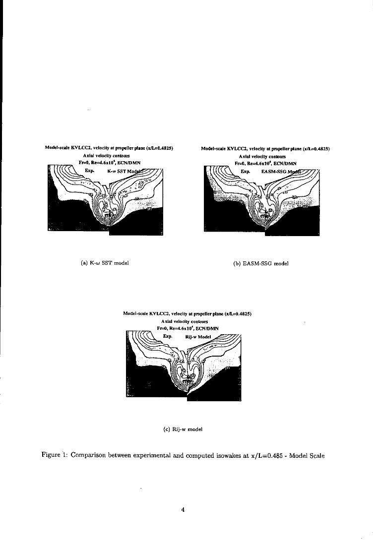
Model-scale KVLCC2, velocity at propeller plane (xIL-0f.4825) Model-scale KVLCC2, velocity at propeller plane (xILO-.4825)

Axial velocity contatas Axial velocity contoursFr=-O, Re=4.6x10', ECN/DMN IF. Re=4.6x10', ECN/IJMN

K.. 1G SSTr Mo AMSG

(a) K to SST mode (b) EASM 550 tmodel

Modelsale KVLCC, vlctyat propele plane (xL-fl4825)

Axial vlcty contour

r-lRe-4.6xl0' ECNIDMN

E P. RU-vw Mode

()Ri- wmode

Figure 1: Comparison between experimental and Computed isowakes at x/L=0.486 - Model Scale

4

Model-scale KVLCC2, pmopeller plane (sJLzO-.4825) Model-scale KVLCCZ, propeller plane (x/L=O0.4825)Turbulent Watteti energy contours Turbulent kinetic energy contourn

Fr=O, Re=4.6xl0', ECN/DMN Fr-O, Re=4.6,slO', ECNIDMN

(a) K-to SST model (b) Rij-w model

Figure 2: Comparison between experimental and computed turbulent kinetic energy contours at x/L=O.485-Model Scale

Model-scale KVLCCZ, velocity at propeller plane (xJL=O1.4825) Model-scale ICVLcc2, propeller plane (x]L=0.4825)Axial velocity contours Turbulent kinetic energy contours

Fr=O, Re=IflxlO', ECNIDMN Fr=", Re=L.OXlO', ECNIDMN

(a) Isowake contours (b) Turbulent kinetic energy contours

Figure 3: Comparison between the K - w SST model and the Rij - to model at x/L=O.485 - Fuill Scale

5

RANS Simulation of Propeller in Oblique FlowOuld M. El Moctar, Volker Bertram

Hamburg Ship Model Basin, elmoctar@hsva.de

Propellers operate most of the time in oblique flow, not only in fast ships where the propellershaft is often inclined due to geometrical restrictions. The deviation from the axial directionin all ships is caused by ship motions in manoeuvring and seakeeping. In addition, the ship'swake always introduces locally oblique flow direction for propeller blades. The oblique inflowchanges the flow conditions at the propeller blades: The angle of attack and relative velocitiesdepend now on the blade position, s. Eq.(1). The oblique inflow causes transverse forces onthe propeller shaft which affect the manoeuvring and stability characteristics of the ship. Thelocal flow conditions are important for the propeller blade design as the cyclic loading of theblades affects fatigue strength.

In the following we consider a four-bladed modern propeller in homogeneous wake at obliqueangles up to 120. We compute propeller forces for various advance numbers to investigate theeffect on the propeller load for oblique inflow. In addition we will discuss the forces on theindividual blades as well as the asymmetry in thrust due to oblique flow. The possible effectsof cavitation will not be considered. There are no experimental data available to validate ourcomputational investigations.

We used the commercial RANS solver COMET, ICCM (1999). The conservation equations formass and momentum in their integral form serve as the starting point. The solution domainis subdivided in a finite number of CV's which may be of arbitrary shape. The integrals arenumerically approximated using the midpoint rule approximation. The discretization in timeused an implicit Euler method. The gradient is calculated using a conservative approximationof second order. The discretized continuity equation is transformed in to a pressure-correctionequation following the SIMPLE algorithm, adapted to colocated grids. The momentum compo-nent equations are linearized using the Picard Iteration scheme. The RNG k-E-Model with wallfunctions models the Reynolds stresses. The discretization and linearization lead to a systemof coupled algebraic equations, solved by a segregated iterative approach. The inter-equationscoupling and non-linearities axe resolved in a predictor corrector scheme within outer iterations,which represent the update of the coefficient matrix and source vector. The solution methodis designed to use unstructured grids with cell-wise refinement. For more details see Demirdzicand Muzaferija (1995), ICCM (1999)

We used here unstructured hexahedral grids with 600,000 cells, El Moctar (1999) Grids werelocally refined at the propeller. The innermost cell thickness was chosen such that on averagey+ = 60. The flow was assumed to be fully turbulent..

The turning of the propeller introduces instationary changes in angle of attack and relativevelocity at each blade making a solution in time domain mandatory. In each time step, thecomplete grid is turned corresponding to the advance of the propeller. The time step corre-sponds to a turn of the propeller of 10. Finer time steps had virtually no influence on averageforces on the propeller. Two full propeller revolutions are required to obtain a stable periodsolution, Fig.2. CPU times were 30h per propeller speed and angle of attack on one PentiumII processor with 500MHz.

In a global fixed coordinate system each blade segment experiences (neglecting the effect ofinduced flows) a velocity V6 under an angle of attack fis, Fig.1.

vo (r,6) = !vcos 6)2 + (irnr + v sin6 cos0)2 + (v sin6 sinO)2 (1)

= tan- 1 Vrnr COS 6 (2)7nr+ vsin 6cose0]

v is inflow speed to the propeller, n its rpm, r the radial coordinate, 6 the angle of attack and0 the blade position. 86 changes with speed.

The nondimensional force coefficients for individual blades defined as follows:

f fz(r, O)dA f(fM(r, 0) y - fy(r, 0). x)dAKtb = p- n2 " D4 , KQb = p" n2. D5 (3)

f fx(r, O)dA f fyf(r, O)dAKflb-- n2- D 4 , Kith= p'n2. D 4 (4)

The integral mean values of the nondimensional forces coefficients for the whole propeller (Kt,KQ, Klf) were obtained by summing over all Nb blades. The deviation of the thrust directionfrom the propeller axis in x made nondimensional with propeller radius R is computed as:

E (r,O) " r " cos (ex = Nb E fr,0) (5)

Nb

The propeller position at y axis was chosen as 0 = 00. The forces acting on the propeller shaftwere not considered.

When the blade runs against the direction of the oblique flow, the angle of attack and thevelocity increase and thus the forces on the blade. Correspondingly, the forces on the bladedecrease in the other half period. The increase above the time mean value of the forces is largerthan the decrease, Fig.4 and 5. As a result the mean thrust and torque coefficients are largerthan in homogeneous axial inflow of same advance number J = v/irnD. These differencesincrease with the obliqueness of the'inflow and the advance number, Fig.6. The forces at thepropeller oscillate with a frequency of n/Nb, Fig.2 and 3. The amplitude of the oscillationsincreases with angle of attack, Fig.4 and 5.

The unsymmetry of the force distribution results in a transverse force f1 perpendicular to thepropeller shaft. This transverse force superimposes to the rudder transverse force and hasan important effect on the manoeuvring behavior of the ship due to the large leverage. Thevertical force fy is for horizontal oblique flow smaller than f, by one order of magnitude. Thepoint where the resulting axial force acts depends on the geometry of the blades. It lies behindalways the reference line of the blade position. Therefore the force maximum has a phase shiftwith respect to the blade position, Fig.4 and 5. The unsymmetry of the force distributionshifts the mean thrust by a distance e to the side where the propeller blades run against theoblique inflow. e increases also with advance number and angle of attack, Fig.7. The shiftof the axial force causes moments about the x and y axes. These moments affect trim andstability, particularly for fast ships with high ratios of propeller thrust to ship weight.Full details will appear in my Ph.D. thesis which will appear in late 2000.

DEMIRDZIC, I.; MUZAFERIJA, S. (1995), Numerical method for coupled fluid flow, heattransfer and stress analysis using unstructured moving meshes with cells of arbitrary topology,Comput. Methods Appl. Mech. Engrg. 125, pp.235-255

EL MOCTAR, O.M. (1999), Numerical investigation of propeller rudder interaction,NuTTS'99, Rome

ICCM (1999), Comet Version 1.04 User Manual, ICCM GmbH, Hamburg

0=00

x0-900 0--2700

06--1800 ý jrn. nD v-sinb- cosOz

Fig. 1: Velocity vectors at blade segment on right-turning propeller

-0.0288.......................-0.0034-

-009. . . . ....... . . . ............................. 03 .......... ........- .........................-0.0294.-0.0.....

-0.0296 .~0.0035.....

-0.0292 ........ .... ................- 0.00369.........

-0.03...............................0

-0.0029 -0.0048

0 0.25 0.5 0.75 1 1.25 I.5 1.75 2 0 90 180 270 360time4perdod 0

Fig.2: Convergence history of K1 ý Fig.3: K1 y during one period

0.06 0.011 ____810 8=1200.05............1 ....0....

0.05.-

0.04 - ..... ..... .... 4 . 0.008 .

Ký 0.035 . ... ..... ................... 000. 6=40

0.031(0 0.0070 .0 2 5 . .... ... ....

0.005 ......... .....0.02.

0.025 0.004

0.01 10.003± 20 360 90 180 270 360 090 180 20 36

00800

FigA4: Thrust coefficient at one blade Fig.5: Torque coefficient at one blade

0.U 0.16r101% &L120

0.5.................... 00.4

0.4. ......... 6 12030.12 ......

0.2 oe,/P 0.08 . ...... ......

0.08 . ......

-0.1 --------------------------0.2 .... .... ........................................ 0.02....

-0.3 0 -__

0 0.2 0.4 0.6 0.8 1 0 0.2 0.4 0.6 0.8 1.1 J

Fig.6: Propeller force coefficients Fig.7: Shift of point of action for thrust

Extended Abstract

Predictions of flow-induced motions offloating rigid-bodies

I. Had•,i, S. Muzaferija 0 , Y. Xing and P. Kaeding b

TU Hamburg-Harburg, AB Fluiddynamik und SchiffstheorieLUmmersieth 90, 22305 Hamburg, Germany

a ICCM, Bramfelder Strasse 164, D-22 305 Hamburg, Germanyb Mittelstr. 16b, 22851 Norderstedt, Germany

Computational fluid dynamics in shipbuilding has been mainly used to predict flows around bodiesmoving with a prescribed velocity and vertical position, and the forces acting on the body do nothave an influence on its motion. However, the motion of floating bodies is a direct consequence ofthe forces acting on it, while at the same time these forces are a function of the body movementitself. Therefore, the prediction of flow-induced body motion is a challenging task. It is relevantfor many applications in ship and ocean engineering (sea-keeping, slamming, etc). In this papera computational procedure for the prediction of motion of floating rigid bodies influenced by aviscous-flow is presented.

Mathematical Model The fluid flow is described by the Navier-Stokes equations. For the move-ment of control volumes, the so-called space conservation low is obeyed. In order to determine thedistribution of air and water, an additional equation for the void fraction of one phase is solved.Both fluids are treated as a single effective fluid whose properties vary in space according to thevolume fraction of each fluid. Motion of a rigid body is entirely described by two vector equations,namely the linear momentum equation for the mass center of the rigid body and the angularmomentum equation for the rigid body. In order to solve these equations one needs to know thedistribution of the pressure and the shear stress at the body surface. These are obtained as thesolution of the Navier-Stokes equations.Numerical Method Discretization of the Navier-Stokes equations is done using a finite volumemethod with control volumes of arbitrary shape. The pressure is predicted using the SIMPLEalgorithm [3]. The interface-capturing method is used to compute flows with free-surfaces. Thesolution domain extends over both air and water. The influence of the surface tension is introducedinto momentum equations through equivalent volume forces. In order to achieve the sharpness ofthe interface between water and air, the HRIC [2] (high-resolution interface capturing) scheme isused. The implicit second-order three-time-level scheme is performed for integration in time.Theaccuracy of the numerical procedure is of second order. Due to nonlinearity of the underlayingequations the procedure for prediction of fluid flow in one time step is iterative. For the predictionof body movements a fully-implicit predictor-corrector procedure is applied, using the iterativenature of the fluid-flow solver. Prediction of the fluid flow is done by the program Comet ofICCM (vww. iccm. de) and the body movement is simulated via user-defined modifications of flowequations, grids and boundary conditions.Simulation of Body-Movement We have employed different strategies to simulate the bodymovement. These possibilities come mainly from the features which are offered by the Cometcode. The influence of the rigid-body on the fluid flow can be taken into account by either:a) Adding the body-acceleration vector to the gravity acceleration in the Navier-Stokes equations.The acceleration is predicted according to the linear momentum equations for the center of massof the rigid body or the angular momentum equations for the rigid body.b) Shifting the computational-domain boundary which is common with the body surface. Thesurrounding grid cells are rearranged so that the grid quality is retained.c) Moving the entire numerical grid or some parts of it. For large angles of rotation, the slidinginterface between a block attached to the body and the rest of computational domain is used. Ifthe grid is moved, spacial care needs to be taken about the computational-domain boundaries.

1

For complex cases it is necessary to combine some of these methods.

Results In this paper we will present results and report on experience while simulating flow-induced rigid-body motions. A number of simple test cases, with translation or rotation only, wasanalyzed first in order to verify the procedure and estimate the numerical accuracy. Applications ofthe method to more complex problems will be presented and the results obtained will be discussed.Some results with animations can be found at: http://ww,.schif fbau.uni-hamburg.de/-ibro/rolls .html.

The impact of a cylindrical shell on water was subject of an experimental investigation con-ducted by (1]. The cylinder, with an outer diameter of 306 mm and wall thickness 3 mm, wasdropped onto the water surface from a height of 75 cm. Figure la shows comparison of measuredand computed positions of the cylinder center as a function of time. The shape of the free surfaceat time t = 0.4871 s together with the pressure distribution is shown in Fig. lb.

Fig. 2a shows free-surface and body position at time t = 0.6s in another test case. The centerof square cylinder is initially located at Y, = 1.25D (D is cylinder width) below the free surfaceand is at rest as well as the fluid itself. The cylinder can move only in the vertical direction.After being released, due to the buoyancy force (density of the body is half of the water density),the body first moves upwards and oscillates towards the equilibrium state. Fig. 2b shows theintegral vertical force F., velocity v, and position Y, of the body center as a function of time.The horizontal lines indicate the equilibrium values. Until t A 2 s the strong dumping of bodymovement due to viscous forces and generation of waves is present and then large oscillations ofbody are caused by the reflection of waves from side walls of the channel. A very complex situationis generated while the body brakes the free surface moving upwards and downwards, as indicatedin Fig. 2a, and in Fig. 2b by rapid change of force F. representing the impingement of water atthe body.

Fig. 3a and b show position and velocity of the center and the angle of rotation and the angularvelocity of an open cylinder falling into still water. The cylinder is partially filled by water and fallsat an inclination of 15 degrees to the water surface. The body has one linear and one rotationaldegree of freedom. Both the slamming and the sloshing occur in such a situation. An amount ofwater flows into cylinder, as shown in Fig. 3c, which influences floating characteristics of the body.

Fig. 4a shows trajectory of the center of a rectangular cylinder falling in water and Fig. 4bshows angular velocity of the body. The angular movement is initiated by the inclined startposition (15 degrees) and the later development is mainly dominated by waves as shown in Fig.4c. The body had all three degrees of freedom which are possible in a two-dimensional simulation.

Fig. 5a and b show comparison of free-surface waves predicted using the Euler scheme and thethree-time-level scheme. Waves are generated by moving sinusoidally a flapping wall at x = 0. Dueto large numerical diffusion the amplitude of waves predicted by the Euler scheme is substantiallydamped. The second-order three-time-level scheme preserves the amplitude of waves much better,at no additional computational cost and only a moderate increase in memory requirements. In Fig.5c the position of a partially submersed square cylinder with only a rotational degree of freedomsubjected to waves is shown. Fig. 5d shows the angular position of the cylinder as a function oftime.

References[1J M. Arai and T. Miyauchi. Numerical study of the impact of water on cylindrical shells, considering

fluid-structure interactions. In M.W.C. Oosterveld and S.G. Tan, editors, Practical Design of Shipsand Mobile Units. Elsevier Science B.V., 1998.

[2] S. Muzaferija and M. Peri6. Computation of free-surface flows using interface-tracking and interface-capturing method. In 0. Mahrenholtz and W. J. Minkowycz, editors, Nonlinear Water Wave Inter-action, pages 59-100. Computational Mechanics Publications, 1999. Chapter 2.

[31 S. V. Patankar and D. B. Spalding. A calculation procedure for heat, mass and momentum transferin three-dimensional parabolic flows. Int. J. Heat and Mass Transfer, 15:1787-1806, 1972.

2

a) I b)A 2 OOQe.03a)~~ C 2-.b 1.5008+03-0, Experiment D 1.4000n 0

S0..8~ -Calculation 11=2XG 8.00+0&2o H 6.6.000802:s 0 .6 1 4 z o2

0.4

• 0.2

0-0.1 0 0.1 0.2 0.3 0.4 0.5 0.6 0.7 0.8 0.9

Time [s]Figure 1: a) Position of cylinder center relative to still water surface; b) free surface and pressurecntures at time t = 0.4871 s. b) o.2

al b 0.24F,

0.1 Y•

0 .1 "-' 2v~ C

-0.

-O I*, , .

Lim0 1 2 3 4 5time (s)

Figure 2: a) flee-surface and body position at time t =0.6 s; b) Integral vertical force F., velocityv, and position Ye of body center in time.

a) 0.1 -O-- .25*V~ b) 0.

' " " - "

IJ

i

0 '• ,-- ' \ / I

.//,,

,-0 .1 I-

0 .2

i-0. -0.2

10 1 2 3 4 5 0 1 2 3 4 5

time (s) time (s)

t = 0.7 s

c)

Figure 3: a) Position and velocity of body center; b) angle and the angular velocity of the body;c) flee-surface and body position at time t = 0.7 s.

3

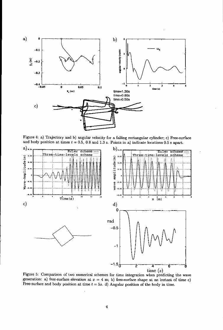
a) 0 b) 2

-0.2

-0.05 0 0.05 0.1 0 1 2 3 4 5

'I (Mn) time-1 .30s

time-O.80s;

c)

Figure 4: a) Tfrajectory and b) angular velocity for a falling rectangular cylinder; c) Free-surfaceand body position at times t = 0.5, 0.8 and 1.3 s. Points in a) indicate locations 0.5 s apart.

a)Ru le b)0.0L 'E u i or s d h e m d -

000

-00.02

1 2 4 6 0 3 00 1 1TiMe (so) x (Mn)

c) d)0

rad

-0.5

-1 5

timne (s)Figure 5: Comparison of two numerical schemes for time integration when predicting the wavegeneration: a) free-surface elevation at x = 4 mn; b) free-surface shape at an instant of time c)Free-surface and body position at time t = 5s. d) Angular position of the body in time.

4

Free-Surface RANSE Computations Employing Parallel Computing Techniques

Dieke Hafermann, Jochen Laudan, Volker Bertram, HSVA, Hamburg, bertram@hsva.deSamir Muzaferija, ICCM, Hamburg, sarnir@iccm.de

Full details on the finite-volume discretization implies that the computed fluxes of volume fractionmethod behind the commercial code COMET used do not underflow or overflow the cells. The HRIChere are given in Demirdzic and Muzaferija (1995), scheme employed here satisfies these conditions,Muzaferija and Peric (1998). We will therefore be Muzaferija and Peric (1998).very brief in outlining the fundamentals of theapproach. Starting from an ICES description of the KRISO

container ship (KCS), www.iihr.uiowa.edu/gothen-We solve the RANSE with a k-E RNG turbulence burg2000/KCS/container.html, a computationalmodel. The conservation equa-tions of mass, grid was generated with the standard grid gene-volume concentrations and momentum are solved ration software ICEM-CFD. The grid consisted ofin time for free-surface flows. In order to solve the several blocks. Initial grids with non-matching gridgoverning equations, the solution domain is first boundaries did not yield plausible results and thesubdivided into an arbitrary number of control reasons for this behavior are not yet understood asvolumes (CVs) or cells. Control volumes can be of other test cases with non-matching boundaries didan arbitrary polyhedral shape allowing for local not exhibit similar problems. A block-structuredgrid refinement, sliding grids, and blocks of grid grid with matching boundaries performed muchwith non-matching block interfaces. In principle, better and the results for this grid are shown here.this simplifies grid generation and enables a more The grid had 446613 cells. The cylindrical grid hadeffective distribution of grid points by clustering a radius of 1.5 Lwp and extended 1 Lpp ahead of FPthem in the regions of strong variation of variables, and 2 LIp behind AP. The region above the calmThe values of all dependent variables are stored in waterline was discretized up to 0.065 Lpw. Thethe center of each CV. innermost cells were such that 20 < y' < 170. The

grid was split into 3 blocks, Fig.1. One blockThe governing equations are integrated over each covered the forward part of the domain, one blockCV. The volume and surface integrals are the aft part below the free surface, and the lastcalculated using second-order approximations block the aft part with fine resolution of the free(linear interpolation, central differences, and surface. The grid on the hull was designed tomidpoint rule integration). The method is fully resolve areas with high gradients in flow quantitiesimplicit, i.e. the spatial integrals are evaluated at finer, Fig.2.the new time level while the old values appear onlyin the approximations of the time derivative. The The computations were performed for modelpressure-correction equation derived from the Reynolds number R,=1.59.107 and Froude numberdiscretized continuity and momentum equations is Fn = 0.26 only for the condition without operatingused to determine the pressure. The resulting propeller. Note that the experiments weresystem of nonlinear and coupled algebraic performed at Rn=I.4.10 7, i.e. the viscosity in theequations is solved iteratively in a sequential computations was higher.manner. The linearized equations are solved usingsolvers from the family of conjugate-gradient At the upstream inlet, we set uniform velocity ofmethods. Iterations are repeated within each time model speed both above and below the calmstep until the nonlinear equations are satisfied waterline. The turbulence intensity of the water waswithin acceptable tolerances. The momentum and set at 3% at the inlet. The characteristic length wascontinuity equations were approximated by a set at 0.4 m. The upper boundary and the center-central differencing scheme, the turbulence plane were defined as planes of symmetry. On theequations by a upwind differencing scheme, ship hull, we enforced the no-slip condition. The k-

E RNG turbulence model employed a wall function.The discretization of the convective part of the The time step interval was set at 0.01s. Within eachvolume fraction conservation equation needs time step, 10 iterations to reduce the residuals werespecial attention. Ideally, its discretization should performed.neither produce numerical diffusion nor unboundedvalues of the volume fraction, i.e. the value of the The convergence criterion was based on pressurevolume fraction in each cell should lie between the and frictional resistance. Fig.3 shows theminimum and maximum value of the neighbor convergence history for the finest grid. The averagecells. The demand for a scheme to be bounded of the oscillatory forces was taken. While the

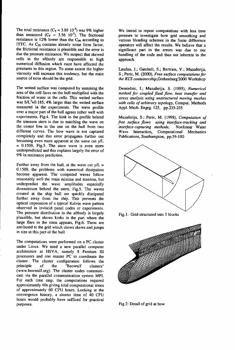
The total resistance (CT = 3.89 10 3) was 9% higher We intend to repeat computations with less timethan measured (CT = 3.56 10-3). The frictional pressure to investigate how grid smoothing andresistance is 12% lower than the CFo according to various blending schemes in the finite differenceIrTC. As CF contains already some form factor, operators will affect the results. We believe that athe frictional resistance is plausible and the error is significant part in the errors was due to ourdue the pressure resistance. We suspect that skewed handling of the code and thus not inherent in thecells in the aftbody are responsible to high approach.numerical diffusion which must have affected thepressures in this region. To some extent the higher Laudan, J.; Gatchell, S.; Bertram, V.; Muzaferija,viscosity will increase this tendency, but the main S.; Peric, M. (2000), Free-surface computations forsource of error should be the grid. the KCS containership,Gothenburg'2000 Workshop

The wetted surface was computed by summing the Demirdzic, I.; Muzaferija, S. (1995), Numericalarea of the cell faces on the hull multiplied with the method for coupled fluid flow, heat transfer andfraction of water in the cells. This wetted surface stress analysis using unstructured moving mesheswas S/L 2--0.185, 4% larger than the wetted surface with cells of arbitrary topology, Comput. Methodsmeasured in the experiments. The wave profile Appl. Mech. Engrg. 125, pp.235-255over a major part of the hull agrees rather well withexperiments, Fig.4. The kink in the profile behind Muzaferija, S.; Peric, M. (1998), Computation ofthe transom stem is due to matching the wave on free surface flows using interface-tracking andthe center line to the one on the hull from two interface-capturing methods, Nonlinear Waterdifferent curves. The bow wave is not captured Wave Interaction, Computational Mechanicscompletely and this error propagates further out Publications, Southampton, pp.59-100becoming even more apparent at the wave cut y/L= 0.1509, Fig.5. The stern wave is even moreunderpredicted and this explains largely the error of9% in resistance prediction.

Further away from the hull, at the wave cut y/L =0.1509, the problems with numerical dissipationbecome apparent. The computed waves followreasonably well the main minima and maxima, butunderpredict the wave amplitudes especiallydownstream behind the stern, Fig.5. The wavescreated at the ship hull are quickly dissipatedfurther away from the ship. This prevents theoptical impression of a typical Kelvin wave patternobserved in inviscid panel codes or experiments.The pressure distribution in the aftbody is largely Fig.l: Grid structured into 3 blocksplausible, but shows kinks in the part where thelarge flare in the stern appears, Fig.6. These areattributed to the grid which shows skews and jumpsin size at this part of the hull.

The computations were performed on a PC clusterunder Linux. We used a new parallel computerarchitecture at HSVA, namely 8 Pentium IIIprocessors and one master PC to coordinate thecluster. The cluster configuration follows theprinciple of the "Beowulf clusters"(www.beowulf.org). The cluster nodes communi-cate via the parallel communication system MPI.For each time step, the computations requiredapproximately 40s giving total computational timesof approximately 60 CPU hours. Looking at theconvergence history, a shorter time of 40 CPUhours would probably have sufficed for practicalpurposes. Fig.2: Detail of grid at bow

Faoo

-60 ---------- _ _ _

- -. - -1 -- --

-100 ---------

0 ID 2 30 40 w06

t (']

Fig. 3: Convergence of resistance; resistance values averaged over oscillations

- - -- - - . -. . - *fl - -

Fig4: Wave profile on hull, ahead and behind transom

aa

.00 =a,% 0 0

Fig.6: Hull pressure contour lines, A Cp= 0.01

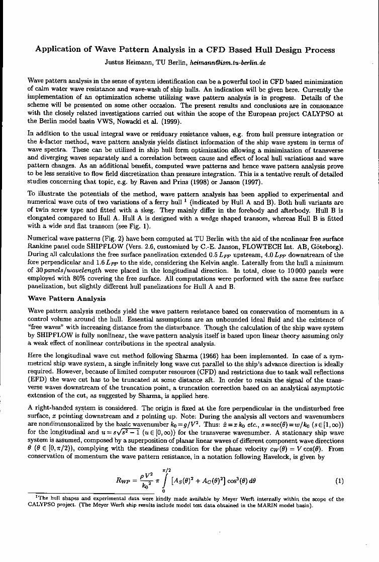
Application of Wave Pattern Analysis in a CFD Based Hull Design Process

Justus Heimann, TU Berlin, heimannfism.tu-berlin.de

Wave pattern analysis in the sense of system identification can be a powerful tool in CFD based minimizationof calm water wave resistance and wave-wash of ship hulls. An indication will be given here. Currently theimplementation of an optimization scheme utilizing wave pattern analysis is in progress. Details of thescheme will be presented on some other occasion. The present results and conclusions are in consonancewith the closely related investigations carried out within the scope of the European project CALYPSO atthe Berlin model basin VWS, Nowacki et al. (1999).

In addition to the usual integral wave or residuary resistance values, e.g. from hull pressure integration orthe k-factor method, wave pattern analysis yields distinct information of the ship wave system in terms ofwave spectra. These can be utilized in ship hull form optimization allowing a minimization of transverseand diverging waves separately and a correlation between cause and effect of local hull variations and wavepattern changes. As an additional benefit, computed wave patterns and hence wave pattern analysis proveto be less sensitive to flow field discretization than pressure integration. This is a tentative result of detailedstudies concerning that topic, e.g. by Raven and Prins (1998) or Janson (1997).

To illustrate the potentials of the method, wave pattern analysis has been applied to experimental andnumerical wave cuts of two variations of a ferry hull 1 (indicated by Hull A and B). Both hull variants areof twin screw type and fitted with a skeg. They mainly differ in the forebody and afterbody. Hull B iselongated compared to Hull A. Hull A is designed with a wedge shaped transom, whereas Hull B is fittedwith a wide and flat transom (see Fig. 1).

Numerical wave patterns (Fig. 2) have been computed at TU Berlin with the aid of the nonlinear free surfaceRankine panel code SHIPFLOW (Vers. 2.6, customized by C.-E. Janson, FLOWTECH Int. AB, Gdteborg).During all calculations the free surface panelization extended 0.5 Lpp upstream, 4.0 Lpp downstream of thefore perpendicular and 1.6 Lpp to the side, considering the Kelvin angle. Laterally from the hull a minimumof 30panels/wavelength were placed in the longitudinal direction. In total, close to 10000 panels wereemployed with 80% covering the free surface. All computations were performed with the same free surfacepanelization, but slightly different hull panelizations for Hull A and B.

Wave Pattern Analysis

Wave pattern analysis methods yield the wave pattern resistance based on conservation of momentum in acontrol volume around the hull. Essential assumptions are an unbounded ideal fluid and the existence of"free waves" with increasing distance from the disturbance. Though the calculation of the ship wave systemby SHIPFLOW is fully nonlinear, the wave pattern analysis itself is based upon linear theory assuming onlya weak effect of nonlinear contributions in the spectral analysis.

Here the longitudinal wave cut method following Sharma (1966) has been implemented. In case of a sym-metrical ship wave system, a single infinitely long wave cut parallel to the ship's advance direction is ideallyrequired. However, because of limited computer resources (CFD) and restrictions due to tank wall reflections(EFD) the wave cut has to be truncated at some distance aft. In order to retain the signal of the trans-verse waves downstream of the truncation point, a truncation correction based on an analytical asymptoticextension of the cut, as suggested by Sharma, is applied here.

A right-handed system is considered. The origin is fixed at the fore perpendicular in the undisturbed freesurface, z pointing downstream and z pointing up. Note: During the analysis all vectors and wavenumbersare nondimensonalized by the basic wavenumber ko =g/V2 . Thus: i = iko etc., s=sec(O) =w/ko (s E [1, oo))for the longitudinal and u = svs s"- 1 (u E [0, co)) for the transverse wavenumber. A stationary ship wavesystem is assumed, composed by a superposition of planar linear waves of different component wave directions0 (0 E [0,7r/2)), complying with the steadiness condition for the phase velocity cw(G) = Vcos(0). Rtomconservation of momentum the wave pattern resistance, in a notation following Havelock, is given by

R pV 2 f/ 02 ()2 3()dWP- = 7r ] [As() 2 +A(OC) 2 ] cos3 (6)dO (1)

'The hull shapes and experimental data were kindly made available by Meyer Werft internally within the scope of theCALYPSO project. (The Meyer Werft ship results include model test data obtained in the MARIN model basin).

and the wave pattern resistance coefficient is defined as (SRhf: wetted hull surface area at rest)

Rwp 7rCwp = 0.5 pSRý! V 2 or Cwp(O) = 0.5[As() 2 + Ak()] cos3 (). (2)

As and Ac in (1) and (2) are called the free wave spectra

As(O) = I [S*(s, ) cos(ul) + C*(s,b) sin(uý)], Ac(O) = [S(sO)sin(u4) -C(5,9)cos(n 1 (3)

and S* and C* denote weighted Fourier transforms

S* = J V•-I /(,-)) sin(st)d5a, C*(s,D)= f V'sI(&i,•j) cos(si)d1, (4)-- 0 •00d

with v -1 being the "weight" and ,)(t, g) the wave signal at (9 =const.). Special assumptions are neededin order to account for the signal of the transverse waves beyond the truncation point i. Sharma suggeststhe following approach to analytically extending the wave cut infinitely downstream

C(, cos(,) - C2 sin() for & -+ oo, (5)

where the coefficients c1,2 ,3 are determined by fitting (5) to the tail end of the wave cut signal up to &e. Thecontribution of the integration 4e <1 < oo then can be derived by evaluation of (4) with the wave signalreplaced by (5) and the integration bounds adapted accordingly. Because of the strong asymptotic decay ofthe wave elevation for t -- -oo, according to Sharma, practically no correction is needed to account for thetruncation of the wave cut upstream.

The application of longitudinal wave cut analysis mainly depends 1. on the lateral distance of the cut, 2.on the utilizable length of the signal until truncation and 3. on the speed of the ship or wavenumber. Thefirst two influences are in opposite direction. In order to fulfill the requirement of a free wave system, thecut has to be far enough aside of the ship to be virtually free of local wave effects. On the other hand, thegreater the lateral distance, the shorter is the utilizable signal before truncation due to the effects of tankwall reflections. From a practical point of view, the lateral distance of the cut should be as small as possiblein order to retain as much information as possible of the wave signal. But, still a minimum lateral distanceof the wave cut has to be maintained. Tests indicate that stable analysis results are to be expected alreadyat a minimum distance of y/Lppz0.2, provided that the cut extends far enough downstream (several timesthe basic wavelength). This is in agreement with similar investigations, e.g. Lalli et al. (1998).

Results

In Fig. 4 measured (MARIN) and computed (SHIPFLOW) longitudinal wave cuts at y/Lpp = 0.1814 arecompared for both hull variants and different Froude numbers. A close correlation between measured andcomputed wave cuts beside the hulls (0 /< xLpp < 1.5) can be noted. In the downstream region (x/Lpp > 1.5),the computed wave amplitudes are too large when compared to the measurements. Because of the absence ofviscous damping the stern waves are overestimated here within the computations, which is typical for Rankinepanel methods. This effect is amplified with increasing F.. In addition a phase shift of the calculated wavestowards increasing wavelengths can be noticed. This defect appears to be more present with decreasing F.and in case of Hull B. The latter might be explained by a deviation of trim and sinkage between experimentsand computations, which was present only in the case of Hull B. That again might be caused by the largetransom of Hull B compared to A or perhaps by a different realization of the trials in the experiments andcomputations.

The wave cuts presented in Fig. 4 have been analyzed by means of wave pattern analysis. A proper analysisrequires a "clean" wave cut free of reflections as they originate from tank walls in experiments. Such undesiredinteractions are present in the measured wave cuts at x/Lpp > 3.0 and for lower F.. For that reason, wavesignals have been considered consistently in the analysis only up to an estimated truncation point of x/Lpp:<3.9 (F,,=0.36), <3.5 (Fn=0.331) and <2.9 (F&=0.303).

In Fig. 5 the spectral results of the wave pattern analysis are presented in terms of wave pattern resistancecoefficients Cwp(O). The trends (humps and hollows) of Cwp(O) reveal a good overall correlation betweenexperiments and computations, especially at higher F. and for Hull A. The amplitudes of Cwp(O) appear tobe greater in case of the computations than for the experiments, particularly in the range of the transverse

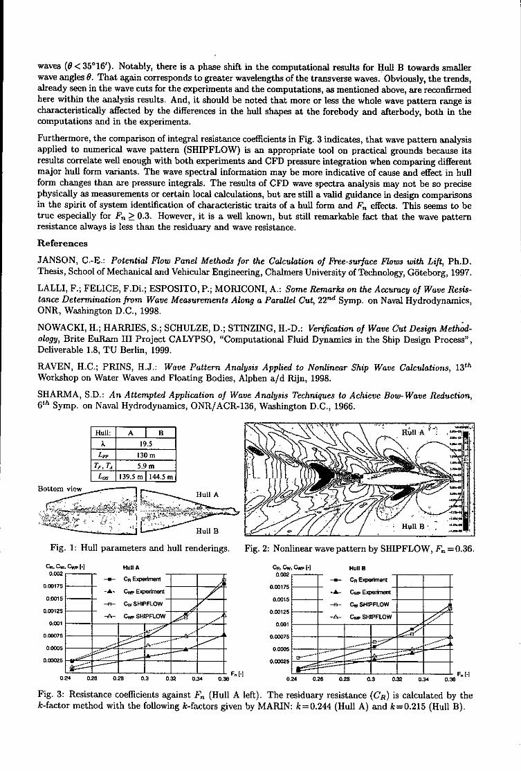
waves (0 < 35'16'). Notably, there is a phase shift in the computational results for Hull B towards smallerwave angles 0. That again corresponds to greater wavelengths of the transverse waves. Obviously, the trends,already seen in the wave cuts for the experiments and the computations, as mentioned above, are reconfirmedhere within the analysis results. And, it should be noted that more or less the whole wave pattern range ischaracteristically affected by the differences in the hull shapes at the forebody and afterbody, both in thecomputations and in the experiments.

Furthermore, the comparison of integral resistance coefficients in Fig. 3 indicates, that wave pattern analysisapplied to numerical wave pattern (SHIPFLOW) is an appropriate tool on practical grounds because itsresults correlate well enough with both experiments and CFD pressure integration when comparing differentmajor hull form variants. The wave spectral information may be more indicative of cause and effect in hullform changes than are pressure integrals. The results of CFD wave spectra analysis may not be so precisephysically as measurements or certain local calculations, but are still a valid guidance in design comparisonsin the spirit of system identification of characteristic traits of a hull form and F. effects. This seems to betrue especially for F. > 0.3. However, it is a well known, but still remarkable fact that the wave patternresistance always is less than the residuary and wave resistance.

References

JANSON, C.-E.: Potential Flow Panel Methods for the Calculation of Free-surface Flows with Lift, Ph.D.Thesis, School of Mechanical and Vehicular Engineering, Chalmers University of Technology, G6teborg, 1997.

LALLI, F.; FELICE, F.Di.; ESPOSITO, P.; MORICONI, A.: Some Remarks on the Accuracy of Wave Resis-tance Determination from Wave Measurements Along a Parallel Cut, 22nd Syrup. on Naval Hydrodynamics,ONR, Washington D.C., 1998.

NOWACKI, H.; HARRIES, S.; SCHULZE, D.; STINZING, H.-D.: Verification of Wave Cut Design Method-ology, Brite EuRamn III Project CALYPSO, "Computational Fluid Dynamics in the Ship Design Process",Deliverable 1.8, TU Berlin, 1999.

RAVEN, H.C.; PRINS, H.J.: Wave Pattern Analysis Applied to Nonlinear Ship Wave Calculations, 1 3 th

Workshop on Water Waves and Floating Bodies, Alphen a/d Rijn, 1998.

SHARMA, S.D.: An Attempted Application of Wave Analysis Techniques to Achieve Bow-Wave Reduction,6 th Symp. on Naval Hydrodynamics, ONR/ACR-136, Washington D.C., 1966.

Hull: A B Run

X 19.5LPP 130 m

TF, TA 5.9 m4,s 139.5 m 1144.5 i

Bottom view -. l

Hull B I H -B1

Fig. 1: Hull parameters and hull renderings. Fig. 2: Nonlinear wave pattern by SHIPFLOW, F, = 0.36.

C.. Cw. 0G. 1] Hull A CR, Cw, Cp H Hull B0.002 0,002

R Experhmnt CnA EV'rb0.0175 0.00175 -

-A- Cvp Expermnent 05- Cv.. Experment0.0015 0.0315 -

C, SHIPFLOW -- C, "IPFLOW0.XD125 •-A- C".- SHIPFOWLOW

0.001 *W0.001 _ -

0.0D075 - • 0.03075................................ .................. .. ......

0.0005 ____0.0005

o.o025 F-• ... . 0.00025 .... . ........ ... F

0.24 0. 0.26 0.3 0.32 0o 0.3 - 0.24 0.26 0.2 0.3 0.32 0.34 0.36

Fig. 3: Resistance coefficients against F. (Hull A left). The residuary resistance (CR) is calculated by thek-factor method with the following k-factors given by MARIN: k=0.244 (Hull A) and k=0.215 (Hull B).

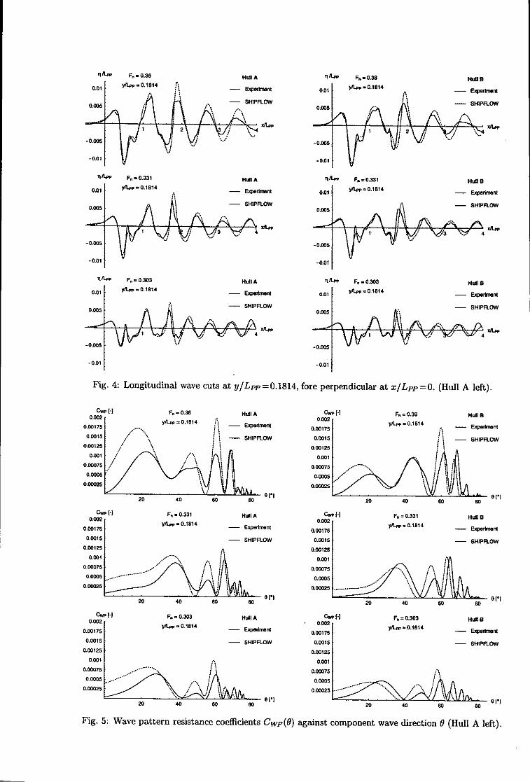
9 F, - 0.38 M, AIitn F. o .38SU

- sMoPROw

-0.015

til. F., M MW A.3 iAý Fý..M =oIni

-SHIPFLOW -SOFO

-0..01

F.I- 0,3 0.3 HuIMA CnpH F..0.30 Hulla

0.0017 y/tp=0.114 f - pSVtT~flt 0.0017 y/Lp..=0.l8I ExperkmMn

0.005 .. i sii a w r SHIPFLOWW5- KIR

-0.001 / I0.001

0.0F00F. = I'W HWI A, 0. [ 005WH0 . W 2Y , . .8 4O52y

" 0 1 1

0.0025 0.125

oilS 0iýi20 40 N0 80 20 40 W0 N

CwH F,.-0.331 HuI A Cw,&H F.0.331 Htd] B-. A, 0.1814 - xprW2n yA.. 0.1814 - Epomn0,0175 0 Sff .0175

0.0015 - SHIPFIOW 0.015 -SH!PFLOW

000125 ,, .0125

000075 -I0.0075

000025~~.ý .1 AA~on.....-- \'A1 sri(20 40 60 80 20 40 W0 W

CwpI F,,0.303 HtuIIA CwU F = 0.303 HWIla0.0017 yA,.q0.1814 - O~rrn .007 y&,=0.1614-

0.001 - SNIPFLOW 0.001 - SI4IPFLOW0.00125 000125

0.0075 ... 00..0t0.750.0005 .- '... 005 -

0,0025 0002.\ /

40 60 80M

Fig. 5: Wave pattern resistance coefficients Cwp(O) against component wave direction 0 (Hull A left).

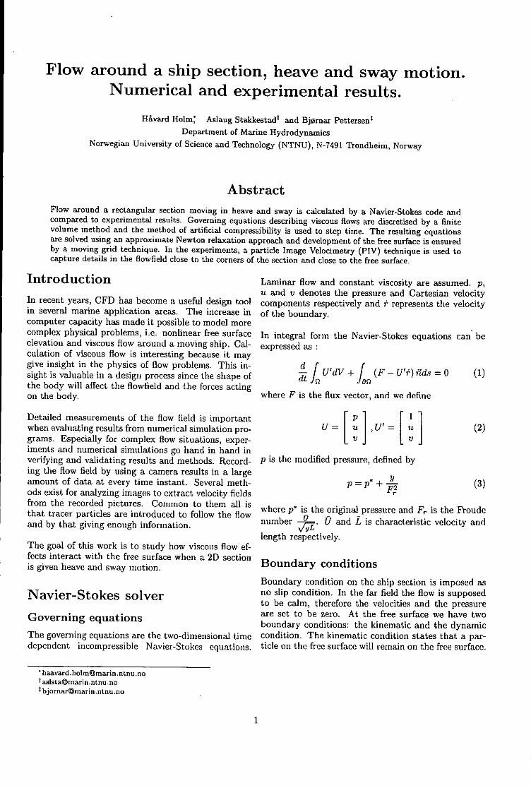
Flow around a ship section, heave and sway motion.Numerical and experimental results.

HAvard Holm, Aslaug Stakkestadt and Bjornar Pettersent

Department of Marine HydrodynamicsNorwegian University of Science and Technology (NTNU), N-7491 Trondheim, Norway

AbstractFlow around a rectangular section moving in heave and sway is calculated by a Navier-Stokes code andcompared to experimental results. Governing equations describing viscous flows are discretised by a finitevolume method and the method of artificial compressibility is used to step time. The resulting equationsare solved using an approximate Newton relaxation approach and development of the free surface is ensuredby a moving grid technique. In the experiments, a particle Image Velocimetry (PIV) technique is used tocapture details in the flowfield close to the corners of the section and close to the free surface.

Introduction Laminar flow and constant viscosity are assumed. p,u and v denotes the pressure and Cartesian velocityIn recent years, CFD has become a useful design tool components respectively and t represents the velocity

in several marine application areas. The increase in of the boundary.computer capacity has made it possible to model morecomplex physical problems, i.e. nonlinear free surface In integral form the Navier-Stokes equations can' beelevation and viscous flow around a moving ship. Cal- expressed asculation of viscous flow is interesting because it maygive insight in the physics of flow problems. This in- d fsight is valuable in a design process since the shape of U'dV + 0 (1)the body will affect the flowfield and the forces acting we n

on the body. where F is the flux vector, and we define

Detailed measurements of the flow field is important [P1 I 1 2when evaluating results from numerical simulation pro- U= 1 u 1 ,U= 1 u (2)grams. Especially for complex flow situations, exper- v viments and numerical simulations go hand in hand inverifying and validating results and methods. Record- p is the modified pressure, defined bying the flow field by using a camera results in a largeamount of data at every time instant. Several meth- p = p* + - (3)ods exist for analyzing images to extract velocity fields r

from the recorded pictures. Common to them all is where p* is the original pressure and F, is the Froudethat tracer particles are introduced to follow the flow nmere p i and ir ist vty andeand by that giving enough information. number7 . U and L is characteristic velocity and

length respectively.The goal of this work is to study how viscous flow ef-fects interact with the free surface when a 2D sectionis given heave and sway motion. Boundary conditions

Boundary condition on the ship section is imposed asNavier-Stokes solver no slip condition. In the far field the flow is supposed

to be calm, therefore the velocities and the pressureare set to be zero. At the free surface we have twoGoverning equations boundary conditions: the kinematic and the dynamic

The governing equations are the two-dimensional time condition. The kinematic condition states that a par-dependent incompressible Navier-Stokes equations. ticle on the free surface will remain on the free surface.

* haavard.holmflmarin.ntnu.notaslsta~marin.ntnu.not bjornarOmarin.ntnu.no

The dynamic boundary condition states that the stresstensor should be continuous over the free surface. Sur-face tension and viscous effects at the free surface areneglected, which results in zero stress tensor. Due to "-•'the zero tangential stress condition, the velocity bound- I <-.inge m.,•i•t....in

ary condition is zero gradient extrapolation. The zero tnormal stress condition lead to the Dirichlet conditionfor pressure on the free surface : p = pn + h/F,, wherep, is the atmospheric pressure and h is the wave height. r, . . . - -

Spatial discretisation and time integra- 'ay

tion

A finite volume method is used to discretize the do- Figure 1: Schematic description of the PIV system.main. The spatial discretization is divided into a vis-cous part and an inviscous part. F~j8 is calculatedusing a central differencing scheme and Ft,,, is calcu- particle will be given at least 5 light pulses and will belated using Roe's upwind scheme with second-order dif- recorded at least 5 times in one image. This mode offerencing. A fully implicit time integrating scheme is recording images is called autocorrelation mode.used. The scheme can be rewied in Hoim and Pettersen[1]. A computer program is used to analyze the images andgive as a result the velocity vectors (2].

Evolution of the free surfaceTo step the free surface in time, the kinematic bound- Experimental setupary condition is used. Traditionally the boundary con-dition is rewritten to 12h = v -Ou h. For a cell centeredat aExcitatordiscretisation v and u are usually taken as the averageof the cells on the left and right hand side closest tothe free surface. 2h is usually calculated using a higherorder upwind scheme. Lw,-dimerssonai

The method has been used with success for a widerange of applications. V

Experimental measurements with L .... ....Particle Image Velocimetry (PIV) la--- --

inl fr1. to, th sideWhen using PIV to study the two-dimensional flow,small seeding glass particles (nearly neutral buoyant), Figure 2: Heave excitation of ship sectionwith average particle diameter of dj = 41.6prm, areadded to the fluid. The fluid is illuminated by a thin, Figure 2 shows the model of the rectangular ship crosspulsating laser sheet. The puls separation is 5t4. Ev- section and how it is forced into heave motion [3]. Theery fluid particle will move a certain distance, Asi, dimensions of the section are shown in the figure. Theduring a given time interval, At. See figure 1. Theprinciple of PIV is to measure this distance, Asi. The experiments were conducted in a research wave flumeprincple ofluid voity vtomeaure U is disthenclcute, As' T special built for visualization and detailed measure-local fluid velocity vector, Uj, is then calculate from ments. The bottom and side walls are all of glass.

S= Asi/At. For sway motion, the same setup was used, turned 900

At is equal to the time between each laser light pulse, with small modifications.

6tp. It is assumed that the particles follow the flow,and that the velocity of the particles is equal to the Computer analysis of imagesvelocity of the fluid. Figure 3(a) shows an image where every particle is

recorded 5-6 times with 12ms interval. To find theA camera is used to capture images of the flow with fluid velocities, U(x,z), from this image, the particlethe illuminated particles. The camera records the po- displacement, As(x, z), has to be found first. The im-sition of each particle at each light pulse. At least two age is divided into small parts called interrogation areaspulses (or particle positions) must be recorded on each (IA), see figure 3(b). It is assumed that the velocity isimage. In the present experiments the time between constant within each IA. As is then found by comput-each light puls was set to 12ms and the camera shutter ing the statistical most probable As in each IA, usingspeed was set to 1/15s (66ms). This means that every

2

the autocorrelation function principles. Several images were recorded at the same time instantin the oscillation period (see figure 4) in separate runsto assure that the repeatability was good.

Figure 5 and 6 shows two images recorded with auto-•, correlation mode. Figure 7 and 8 shows the computer

analysis of the two images respectively, and figure 9and 10 show the numerical calculations. In image 1

MIN_ (figure 5,7 and 9) the section is on its way up. Thevelocities in the measurement area are relatively high.The fluid is sucked under the bottom of the section,

W and a strong vortex is generated. This is clearly shownin the numerical calculations. In image 2 (figure 6, 8

Figure 3: (a): Image recorded with autocorrelation and 10) the section is on its way down, and a relativelymode. The shutter speed is 1/15s (66ms) and the laser large vortex has been formed at the side of the section.scan period is 12ms, allowing 5-6 positions of each par-ticle to be recorded on the image. (b): Example ofinterrogation area (IA).

Errors in PIV

The errors involved in these PIV measurements canbe divided into three main parts. First, errors due tothe physics of the measurement principle. We assumethat the particles follow the flow and that the velocitywithin each IA is constant. This is not true if the veloc-ity gradient is high within an IA. We have to considerthis when choosing size of the IA. Second, recordingerrors. The results from the image analyzing process Figure 5: Picture 1is highly dependent on the quality of the image. Theseerrors are due to the laser light system, camera andlense. Third, analysis errors. These errors include:digitalization/calibration errors, errors related to theautocorrelation and to the autocorrelation peak find-ing process.

Ship section in heave

motion.•

unage2 Figure 6: Picture 2

Figure 4: Numbering of nodes and cells ii •i::iiii::!iii "

Figure 4 shows the measured heave motion for the sec-; • *° ' - r""tion. The figure also show at which points in the oscil- :••!'" z::• ": ' . : : :- . : •'lation the images presented here are taken. The oscil- :• • 7'••. ...lation amplitude is set to 4cm. The oscillation period...- " *:-"... " :

is 0.8 sec. An upstart period of 2 sec, is also numeri-cally sim ulated. (Startup is a separate iss .ue).F g r : A a y e i t r

3

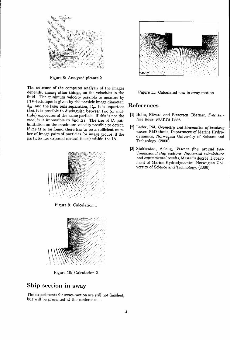
.. f

Figure 8: Analyzed picture 2

The outcome of the computer analysis of the imagesdepends, among other things, on the velocities in the Figure 11: Calculated flow in sway motionfluid. The minimum velocity possible to measure byPIV-technique is given by the particle image diameter,dpi, and the laser puls separation, itp. It is important Referencesthat it is possible to distinguish between two (or mul-tiple) exposures of the same particle. If this is not the [11 Holm, HAvard and Pettersen, Bjornar, Free sur-case, it is impossible to find As. The size of IA puts face flows, NUTTS 1999.limitation on the maximum velocity possible to detect. [2] Lader, P51, Geometry and kinematics of breakingIf As is to be found there has to be a sufficient num- waves, PhD thesis, Department of Marine Hydro-ber of image pairs of particles (or image groups, if the dynamics, Norwegian University of Science andparticles are exposed several times) within the IA. Technology. (2000)

[3j Stakkestad, Aslaug, Viscous flow around two-, .. dimensional ship sections. Numerical calculations

S and experimental results, Master's degree, Depart-.ment of Marine Hydrodynamics, Norwegian Uni-

versity of Science and Technology. (2000)

Figure 9: Calculation 1

Figure 10: Calculation 2

Ship section in swayThe experiments for sway-motion are still not finished,but will be presented at the conference..

4

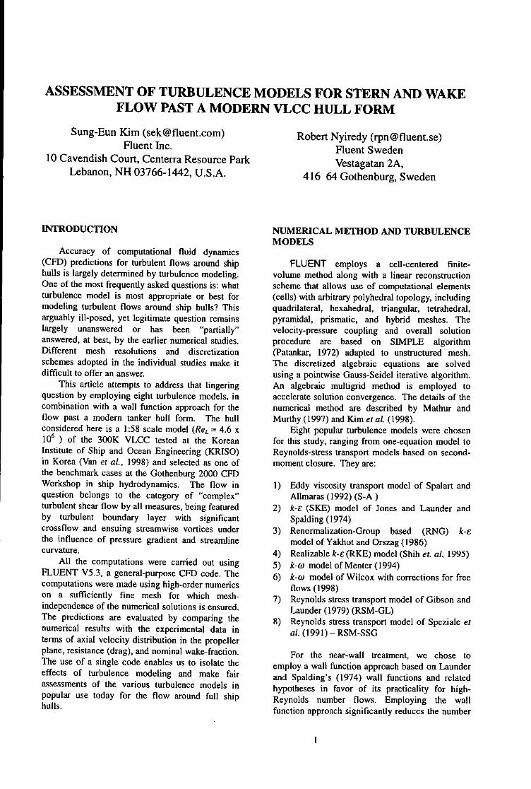
ASSESSMENT OF TURBULENCE MODELS FOR STERN AND WAKEFLOW PAST A MODERN VLCC HULL FORM

Sung-Eun Kim (sek@fluent.com) Robert Nyiredy (rpn@fluent.se)Fluent Inc. Fluent Sweden

10 Cavendish Court, Centerra Resource Park Vestagatan 2A,Lebanon, NH 03766-1442, U.S.A. 416 64 Gothenburg, Sweden

INTRODUCTION NUMERICAL METHOD AND TURBULENCEMODELS

Accuracy of computational fluid dynamics(CFD) predictions for turbulent flows around ship FLUENT employs a cell-centered finite-hulls is largely determined by turbulence modeling, volume method along with a linear reconstructionOne of the most frequently asked questions is: what scheme that allows use of computational elementsturbulence model is most appropriate or best for (cells) with arbitrary polyhedral topology, includingmodeling turbulent flows around ship hulls? This quadrilateral, hexahedral, triangular, tetrahedral,arguably ill-posed, yet legitimate question remains pyramidal, prismatic, and hybrid meshes. Thelargely unanswered or has been "partially" velocity-pressure coupling and overall solutionanswered, at best, by the earlier numerical studies, procedure are based on SIMPLE algorithmDifferent mesh resolutions and discretization (Patankar, 1972) adapted to unstructured mesh.schemes adopted in the individual studies make it The discretized algebraic equations are solveddifficult to offer an answer. using a pointwise Gauss-Seidel iterative algorithm.

This article attempts to address that lingering An algebraic multigrid method is employed toquestion by employing eight turbulence models, in accelerate solution convergence. The details of thecombination with a wall function approach for the numerical method are described by Mathur andflow past a modern tanker hull form. The hull Murthy (1997) and Kim etal (1998).considered here is a 1:58 scale model (ReL = 4.6 x Eight popular turbulence models were chosen106 ) of the 300K VLCC tested at the Korean for this study, ranging from one-equation model toInstitute of Ship and Ocean Engineering (KRISO) Reynolds-stress transport models based on second-in Korea (Van et al., 1998) and selected as one of moment closure. They are:the benchmark cases at the Gothenburg 2000 CFDWorkshop in ship hydrodynamics. The flow in 1) Eddy viscosity transport model of Spalart andquestion belongs to the category of "complex" Allmaras (1992) (S-A)turbulent shear flow by all measures, being featured 2) k-c (SKE) model of Jones and Launder andby turbulent boundary layer with significant Spalding (1974)crossflow and ensuing streamwise vortices under 3) Renormalization-Group based (RNG) k-cthe influence of pressure gradient and streamline model of Yakhot and Orszag (1986)curvature. 4) Realizable k-c (RKE) model (Shih et. al, 1995)

All the computations were carried out using 5) k-co model of Menter(1994)FLUENT V5.3, a general-purpose CFD code. The 6) k-ao model of Wilcox with corrections for freecomputations were made using high-order numerics flows (1998)on a sufficiently fine mesh for which mesh- 7) Reynolds stress transport model of Gibson andindependence of the numerical solutions is ensured. Launder (1979) (RSM-GL)The predictions are evaluated by comparing the 8) Reynolds stress transport model of Speziale etnumerical results with the experimental data in al. (1991)- RSM-SSGterms of axial velocity distribution in the propellerplane, resistance (drag), and nominal wake-fraction. For the near-wall treatment, we chose toThe use of a single code enables us to isolate the employ a wall function approach based on Laundereffects of turbulence modeling and make fair and Spalding's (1974) wall functions and relatedassessments of the various turbulence models in hypotheses in favor of its practicality for high-popular use today for the flow around full ship Reynolds number flows. Employing the wallhulls. function approach significantly reduces the number

of cells and the computational effort, inasmuch as Figure 2 shows the contours of the axial velocitythe viscosity-affected near-wall region does not and the crossflow velocity vectors in the propellerneed to be resolved and instead can be bridged by plane predicted by the eight turbulence models. Thethe wall functions. degree to which the predictions capture the unique

Block-structured hexahedral meshes were shape (rabbit's ears) varies widely among theemployed. Grid-convergence of numerical solutions turbulence models employed. Among others, the S-was ensured with three different sizes of meshes. A model and the SKE model fail to capture theThe results presented in this article were obtained characteristic shape. The crossflow and subsequentusing a 2 00,000-cell mesh, for which y+ at the wall roll-up of the vortex sheet is significantlyadjacent cells is in the range of 30 - 80 over most underpredicted by these models. More recentlyof the hull surface. proposed two-equation model such as RKE, RNG,

and k-ai models perform appreciably better than theRESULTS first two models in that they yield stronger

crossflow and more pronounced roll-up. Yet thereStern and wake flow structure are still a substantial gap between the predictions

and the measurement. The result of the k-rn modelOne of the most outstanding features of the by Wilcox stands out among the group of theflow around the subject hull form is the streamwise isotropic eddy-viscosity based models, quite closelyvortices emanating from the stern boundary layer, reproducing the rabbit's ears. The best result,which are a consequence of the crossflow in the however, is obtained by the Reynolds stressboundary layer driven by transverse pressure transport models. The two RSM models are seen togradient. The surface boundary layer carrying faithfully reproduce the rabbit's ears in thecrossflow leaves (separates from) the hull surface in contours. This is quite remarkable andthe form of a free vortex-sheet, being rolled up as it encouraging, considering that wall functions areis convected downstream. The fidelity with which employed in the calculations.the location and strength of the streamwise vorticesare predicted is of great interest to CFDpractitioners in ship hydrodynamics, since the Velocity at propellarplane (x/L - 0.4825)vortices have significant impacts on the fesistance Axial velocity contour (left) and cross-flow vectors

FLUENT results (Spalan-Allmaras)

The streamwise vortices can be visualized mostconveniently via axial velocity contours and -crossflow velocity vectors on transverse planes.The contours of the measured axial velocity in the . " "- .propeller plane are shown in Figure 1. Thecontours feature a very unique shape that resembles 1 , INrabbit's ears. - "

KVL002 ve~olty field at propeller plane (SL 0.35 Velocity at propeller plane (x/L - 0.4825)KV LO2 tFe.ld t orlne Axialvelcltycontour (left) and cross-flow vectors(Re=4-SxlO. Fr-0.142, KRlSO tnwing-tank data) FLUENT results (Standard k-t)

-0. .

ixnI, IVeoctyatprpelr lne(xL 0485

- 0•0 5 F L E T r s ltA k'

0 A 0 -0.04 -0.0 0.5 mrp e ll velocity atparopellnrelane (xr. -0.4825)DAD"" Axil velOlto left) and cross-flowvect2rs40"; :•,;,•' ;I•i FLUENT results (RNG k-e}

-.oae -o.05 -0.04 -4,0 2, a •

Figure 1. Measured axial velocity contour, at •"" •

propeller plane --0.5 rnf

2

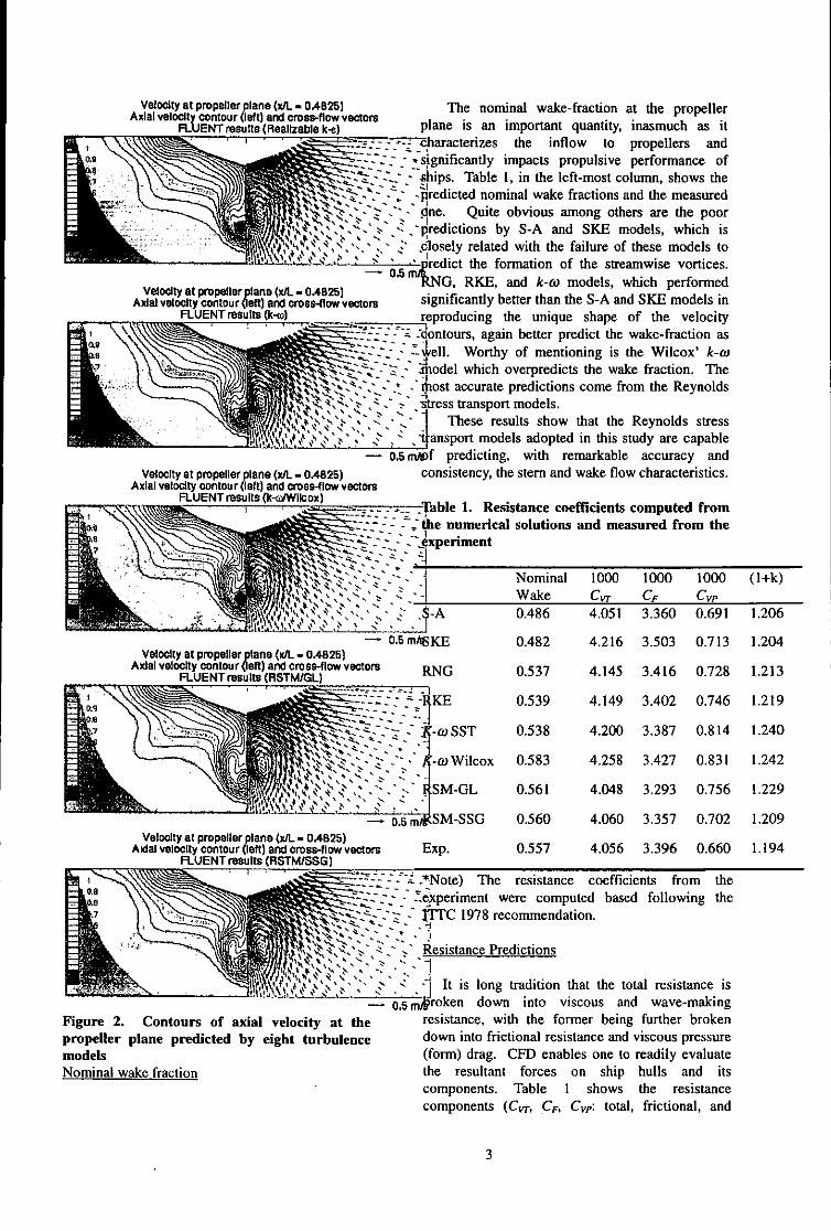
Velocity at propeller plane (xL. - 0.4825) The nominal wake-fraction at the propellerAxial velocity contour (left) and cross-flow vectors

FLUENT results (Realizablek-) plane is an important quantity, inasmuch as itcharacterizes the inflow to propellers andsignificantly impacts propulsive performance ofs- i hips. Table I, in the left-most column, shows the.- " redicted nominal wake fractions and the measureddne. Quite obvious among others are the poor

, predictions by S-A and SKE models, which isclosely related with the failure of these models to

0.-"" -t the formation of the streamwise vortices.

Velocity at propellerplane (xL - 0.4825) 0 G, RKE, and k-on models, which performedAxial velocity contour (left) and cross-fow vectors significantly better than the S-A and SKE models in

FLUENT results (k-c) reproducing the unique shape of the velocity

.". -- ontours, again better predict the wake-fraction as-- -ell. Worthy of mentioning is the Wilcox' k-on

- 'model which overpredicts the wake fraction. The-tost accurate predictions come from the Reynolds

-. "• tr .. rss transport models.,,~'' • 1,.. These results show that the Reynolds stress

,iansport models adopted in this study are capable0.5 mMof predicting, with remarkable accuracy and

Velocity at propeller plane (x/L - 0.4825) consistency, the stern and wake flow characteristics.Axial velocity contour (left) and cross-flow vectorsFLUENT results (k-r WIlc ox)

FLUET reult (k-/Wilox)Table 1. Resistance coefficients computed fromt he numerical solutions and measured from the

-,xperiment

Nominal 1000 1000 1000 (l+k)-1 Wake Cvr CF Cvp

". --•-wy -.'" A 0.486 4.051 3.360 0.691 1.206

0,5 m/SKE 0.482 4.216 3.503 0.713 1.204Velocity at propeller plane (x1L - 0.4825)

Axial velocity contour (left) and cross-flow vectors RNG 0.537 4.145 3.416 0.728 1.213FLUENT results (RSTM/GL)

I KE 0.539 4.149 3.402 0.746 1.219

-_-SST 0.538 4.200 3.387 0.814 1.240

-- -rnWilcox 0.583 4.258 3.427 0.831 1.242

, " .'- " - -.SM-GL 0.561 4.048 3.293 0.756 1.229

• SM-SSG 0.560 4.060 3.357 0.702 1.209Velocity at propeller plane (x/L - 0.4825)

Axial velocity contour (left) and cross-flow vectors Exp. 0.557 4.056 3.396 0.660 1.194FLUENT results (RSTM/SSG)

------' -*Note) The resistance coefficients from the•• e -experiment were computed based following the

-. -- IflC 1978 recommendation.

Resistance Predictions

., It is long tradition that the total resistance is0,staroken down into viscous and wave-making

Figure 2. Contours of axial velocity at the resistance, with the former being further brokenpropeller plane predicted by eight turbulence down into frictional resistance and viscous pressuremodels (form) drag. CFD enables one to readily evaluateNominal wake fraction the resultant forces on ship hulls and its

components. Table I shows the resistancecomponents (Cvr, CF, Cvp: total, frictional, and

3

form drag, respectively) predicted by the 8 Transportation Systems Research Center of theturbulence models along with the measured ones. It KRISO.should be mentioned that the measured totalresistance was analysed following the 1978 ITTC's REFERENCESrecommendation to "derive" the frictional and theviscous pressure resistance coefficients. Van, S.H. et al., Experimental Study on the flow

As shown in the table, all the two-equation characteristics around VLCC with different stem shapes,turbulence models tend to overpredict the total Proc. 3"d International Conference on Hydrodynamicsresistance. Particularly noteworthy is the prediction (ICHD), Seoul Korea, 1998.by the Wilcox' k-rn model which deviates most FLUENT 5 User's Guide, FLUENT Inc., 1998.from the experimental data. The major discrepancycomes from its form drag prediction, which is much Mathur, S.R. and Murthy, J.Y., A Pressure-Basedlarger than the experimental value and those Method for Unstructured Meshes, Numerical Heatpredicted by other models. The predictions by the Transfer, Vol.31, pp. 195-215, 1997.RST models are in best agreements with theexperimental data. It is also noted that RSM-GL Kim, S.-E., Mathur, S.R., Murthy, J.Y., and Choudhury,model gives slightly larger form drag than the D., A Reynolds-Averaged Navier-Stokes Solver UsingRSM-SST model. Unstructured Mesh-Based Finite-Volume Scheme,

The fidelity of the resistance predictions, as AIAA-Paper 98-0231, 1998.demonstrated by the present results, demonstrates Kim, S.-E., Unstructured Mesh Based Reynolds Stressthe efficacy of the wall function approach adopted Transport Modeling of Complex Flows, To be presentedin the present calculations, at 39t Aerospace Science Meeting and Exhibit, Reno,

Nevada, 2001.CONCLUSIONS

Spalart, P. and Allmaras, S., A One-EquationSThe performance of the isotropic eddy- Turbulence Model for Aerodynamic Flows, AIAA Paper92-0439, 1992.viscosity based turbulence models varies in awide range. The Spalart-Allmaras model and Launder, B.E. and Spalding, D.B., The Numericalthe standard k-E model fall short of predicting Computation of Turbulent Flows, Comp. Meth. AppLthe major characteristics of the flows around Mech. Eng., Vol. 3, pp. 269-289, 1974.full hull forms. Some of the more recent two-equation turbulence models including RNG k- Yakhot, V. and Orszag, S. A., Renormalization Groupa realizable k-e, and k-co models tend to Analysis of Turbulence I. Basic Theory, J. Scientificimprove the predictions. However, their Computing, Vol. 1, No. 1, pp. 1-51, 1986performance is mixed. Shih, T.-H., Liou, W.W., Shabbir, A., and Zhu, J.,

o The Reynolds stress transport models give the A New k-c Eddy-Viscosity Model for High Reynoldsbest predictions from the all aspects considered Number Turbulent Flows - Model Development andhere. They not only capture the characteristic Validation, Computers & Fluids, Vol. 24, No. 3, pp.shape of the axial velocity contours 227-238, 1995.successfully but also predict the resistance andthe wake-fraction with remarkable accuracy Menter, F.R., Two-Equation Eddy-Viscosity Turbulenceand consistency. Models for Engineering Applications, AIAA J., Vol. 32,

* The wall function approach adopted in this No. 8, August 1994.study, when combined with accurate numerics Wilcox, D.C., Turbulence Modeling for CFD, 2'"and reliable turbulence models, is capable of Edition, DCW Industries, Inc., 1998.predicting the salient features of the turbulentshear flows around full ships. The results Gibson, M.M. and Launder, B.E., Ground Effects onclearly demonstrate that the wall function Pressure Fluctuations in the Atmospheric Boundaryapproach is a viable choice in the near-wall layer, . Fluid Mech., Vol. 86, pp. 491--511, 1978.modeling of high-Reynolds number flows suchas ship flows. Speziale, C.G., Sarkar, S. and Gatski, T.B., Modeling the

Pressure-Strain Correlation of Turbulence, . FluidACKNOWLEDGEMENTS Mech., Vol. 227, pp. 245-272, 1991.

The authors gratefully acknowledges that the meshused in the present calculations is originallyprovided by the CFD group at the Marine

4

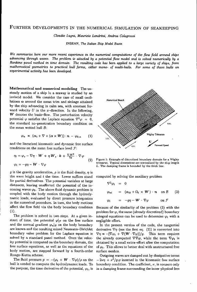
FURTHER DEVELOPMENTS IN THE NUMERICAL SIMULATION OF SEAKEEPING

Claudio Lugni, Maurizio Landrini, Andrea Colagrossi

INSEAN, The Italian Ship Model Basin

We summarize here our more recent experience in the numerical computations of the flow field around shipsadvancing through waves. The problem is attacked by a potential flow model and is solved numerically by aRankine panel method in time domain. The resulting code has been applied to a large variety of ships, frommathematical geometries to practical hull forms, either mono- of multi-hulls. For some of these hulls anexperimental activity has been developed.

Mathematical and numerical modeling The un-steady motion of a ship in a seaway is studied by aninviscid model. We consider the case of small oscil-lations a around the mean trim and sinkage attained NumericaIBeach

by the ship advancing in calm sea, with constant for-

ward velocity U in the x-direction. In the following,

W denotes the basis-flow. The perturbation velocitypotential Wp satisfies the Laplace equation V2' = 0,the standard no-penetration boundary condition on OILthe mean wetted hull B:

+pn = ( +V x (a XW))• - 'o,. (1) Wigleyrdman

and the linearized kinematic and dynamic free surface F Spe

conditions on the mean free surface level T:

77t = We- V71- W + 77 W z. k + V w 2 -V2g (2) Figure 1: Example of discretized boundary domain for a Wigley

trimaran, Typical dimensions are normalized by the ship length~t = -- g77 -- W - •P L. The damping frame is bounded by the thick line.

g is the gravity acceleration, p is the fluid density, 77 isthe wave height and t the time. Lower suffices stand computed by solving the auxiliary problemfor partial derivatives. The potential vanishes at largedistances, leaving unaffected the potential of the in- V Wt = 0

coming waves Voo. The above fluid dynamic problem iscoupled with the body motion through the hydrody- Vnt = (att + £It x W) - n on B (3)

namic loads, evaluated by direct pressure integration Wt = -gr/- W - V7• on 1-in the numerical procedure. In turn, the body motionsaffect the flow field via the body boundary condition Because of the similarity of the problem (3) with the(1). problem for W, the same (already discretized) boundary

The problem is solved in two steps. At a given in- integral equations can be used to determine 'Pt with astant of time, the potential Wjlr on the free surface negligible effort.and the normal gradient Wonjl on the body boundary In the present version of the code, the tangentialare known and the resulting mixed Neumann-Dirichlet derivative V7j (see the first eq. (2)) is converted intoboundary value problem for the Laplace equation is Vt1 = -[V'•t + V(W - V'p)]/g. This term requiressolved by a standard panel method. Once the veloc- the already computed VVW, while the term Vcpt isity potential is computed on the boundary domain, the obtained by a small extra-effort after the computationfree surface equations, as well as the equations of the of Wpt. This allows to better deal with unstructured freebody motion, are stepped forward by a fourth-order surface meshes.Runge-Kutta scheme. Outgoing waves are damped out by dissipative terms

The fluid pressure p = -(Wt + W - VW)/p on the - 2vtl + v2 /g W inserted in the kinematic free surfacehull is needed to compute the hydrodynamic loads. To boundary condition. The coefficient, v, is nonzero onlythe purpose, the time derivative of the potential, Wt, is in a damping frame surrounding the inner physical free

surface. A smooth increase from zero up to an empiri-cally determined maximum value is used.

Figure 1 show a typical computational domain 1.2 - /Aaround a tri-hull made by Wigley forms. An appar- I A

ent feature of the adopted discretization is the use of a A A

non structured grid for the free surface. This is a key 0.,point to easily deal with multi-hulls and transom stern 0.6

and also to allow an easy local mesh refinement.0.4 -- TiDOM

DDG 51 The combatant DDG 51 is an example of a 0.2 A JONSWAPstandard frigate. It is characterized by transom stern, ---- Transient Testand sonar dome at the bow. In fig. 2, we show the typ-ical arrangement of the free surface panels. We use an 1 2 3

unstructured grid in the downstream region, where itis more difficult to follow the ship profile. The transomstern is handled by using a fictitious body to smoothly 14- (,/kA

reconcile the hull with the surface level. Fn --0.19In the developed algorithm, we take advantage from A2 t

the possibility of deducing the (linear) response opera- A A A

tor over a wide range of wavelengths by analyzing the 0.8-ship response to a given compact (in time) wave in- 0.6 TiDOMduced excitation (transient test technique). If a large 0.4 A JONSWAPnumber of frequencies has to be considered, this proce- 0.2 ---- TransientTestdure results in a shorter simulation time with respectto fully 3D frequency domain codes and significantly 0reduces the gap with respect to strip-theory codes. 2 XiL 3

Y 1.2 - ,/A0.8 - ' A -- 2282-

kAA

-.2 F028

00 .8 n_ _ 00 ,

0.4 _13 Z . iOZ 4Z-'----- -•:--•:,A

Ts om 02 Transient TStt0 A .....

-0.5 0 0.5 1 X ,/2 )jL 3

icaltowig tak ofINSEN Reult fom thils andmoreTraditonam Stests Faesre 3 r nTiDOM

i heavem Stem andse pith 04 r eA JONSWAP

Figure 2: Simulation of DDG 51 seakeeping. Top: typia dis- 0.2 an. Tr0nsient Testcretization of the free surface. Bottom: details the discr. iztioneof transom and bow regions .. . . . 15. .. 2 . .25'XL'3

A similar procedure has been employed in the phys-ical towing tank of INSEAN. Results from this andmore traditional tests are summarized in plots 3-4 to- Figure 3: Numerical and experimental DDG 51 seakeep-

ing: heave (3 and pitch (5 response amplitude operator-s forgether with the numerical simulation (solid lines). In Fn = 0.19 and 0.28.the whole, a satisfactory agreement is obtained. We

have to observe, though, a trend to under-estimate the1.4- V•A pitch response at the peak as Fn increases.

1-2 Wigley Ttimaran We consider a prototype of

7 • •multi-hull vehicle made by assembling three parabolic0.. A -(Wigley) hulls. In fig. 5, we report a subset of the

0.6- computations and of the experiments performed forthis hull. We also show the comparison with strip-

0.4 theory computations. We recall that, usually, stan-A JONSWAP0.2 ---- raet Test dard strip-theory codes neglect the interaction between

hulls. This is suitable for catamarans at high speed0 .5 1.5 2 2..5 3 .but is progressively wrong when decreasing Fn and

hull spacings. Therefore, we decided to compare ourcomputations with an improved strip-theory where hullinterference is taken into account (Sbding, private com-

/.27 •A6A4, A munication).I ------ M- -..... The speed of advance is increasing from top down,

Aand plays a relevant role in determining shape and am-0.8 [Fn=0.34 plitude of the response operator. For Fn = 0-2, our0.6- Afully three-dimensional model nicely agrees with the

0.4 TiOM measured data over the entire range of wavelengths A.A JONSWAP The strip theory recovers the correct location of the

0.2 - --- TransientTest two peaks (A/L = 0.85 and 1.2) featured by the re-0' sponse amplitude operator. The corresponding ampli-

S 2 XL 3 tudes are over-predicted and (largely) under-predicted,respectively.As the velocity increases, experiments show an increaseof the first peak and a decrease of the second one (cen-

A4 ter plot). Our model clearly over-predicts the secondSFn= 0.41 peak, which now is halfway between strip-theory and

A three-dimensional results.0.8- At the highest velocity, bottom plot, we recover a good0.6 Tagreement in the high-A range, but the peak for smaller

wavelengths is largely over-predicted. In the strip-A.4 - TiDM theory computations, the second peak almost disap-

0.2 .... Transient Test pears and the response is globally over-predicted.

2 Ji 3 Series 60, Cb = 0.8 We conclude by showing someresults concerning a blunter hull: a Series 60 modelwith block coefficient Cb = 0.8. In this case, we en-

4' kA joyed the availability of a careful set of experiments, •, a- - -t~ - - performed by H. Iwashita at Hiroshima University. An

- - extended discussion concerning this cooperative effort011'A--u will be given at the workshop. In figure 6, we compare

numerical and experimental transverse cuts of radiatedwave field during forced heave motion (top plot) and

0.5- TiD.M the corresponding heave added mass and damping co-A JONSWAP efficients. A good agreement is generally obtained.

-.-.-. Transient Test

Discussion Some results by a seakeeping code un-

2 L der continuous improvement have been presented and

compared with experimental data.So far, the numerical method appears as robust and

Figure 4: Numerical and experimental DDGJ 51 seakeep-ing: heave (3 and pitch (5 response amplitude operators for accurate as other three-dimensional seakeeping codesFn = 0.34 and 0.41. in frequency domain. With respect to those, a signifi-

cant speed-up has been achieved by exploiting the idea

15 /kA

A * Exper. Data (INSEAN)2.5 -o- Strip Theory (Soding) 1.5 TIA, - RPM (TiDOM., sin)

TiDOM - RPM (TiDOM, cos)2 • - Exp. Data

1.5

Fn0.A

4

0.500

--- Strip Thoery (S~iding)

2.52

2

0 -- 0.iDO

1.5 Fn 0.31.6 A,,/ pV' •i s TiDOM

051.4 A Exp.Data

0.5 1 1'.5 2 2!5' '3 ?/L 3.5

4.5 /kA1.3

51.5

I A A

2.5 • •0.9

2.5

2 0 n -- . .5 10 i t I 20 i t i t 3

0.5 --.-- SriTheory 1S diAg

SD-TiDOM

0 , 1.3

1.5 2 2.5 3 3.5 -,TiDOM

Figure 5: Wigley Tr~imaran: numerical prediction of pitch re- A Exp.Datasponge amplitude operator for F = 0.2 and 0.4.

of transient tests.Computations and experiments for a mathematical 0.5

tri-hull provide an example where the (still faster) •strip-theory experiences difficulties, probably relatedto the neglected three-dimensional effects.

A carefull comparison with and extensive set of mea- , I I ,,

surements provided by H. Iwashita for a blunt Series •02 0 KL60, Cb = 0.8, is under development and will be dis-

cussd atthe orksop.Figure 6: Series 60 Cb = 0.8. Top plot: longitudinal cut of theradate wve attrnduring forced heave motion (w 2L/g = 7).

The research activity of the first three authors is supported by Center and bottom pits: added mass and damnpiing coefficientsthe Italian Minister, dci Trasporti e delia Navigazione through for heave. Experiments have been performed by H. Iwashita atINSEAN Research Program 2000-2002. the Hiroshima University.

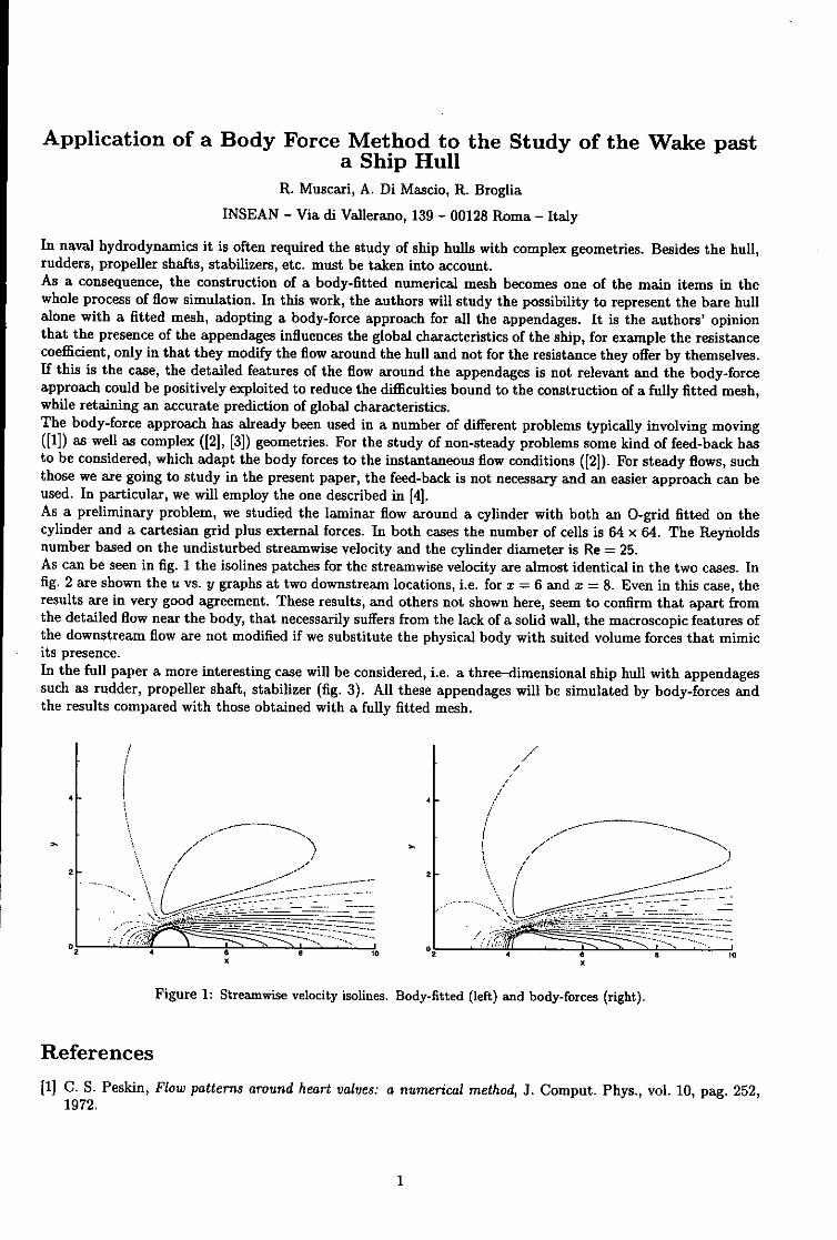
Application of a Body Force Method to the Study of the Wake pasta Ship Hull

R. Muscari, A. Di Mascio, R. Broglia

INSEAN - Via di Vallerano, 139 - 00128 Roma - Italy

In naval hydrodynamics it is often required the study of ship hulls with complex geometries. Besides the hull,rudders, propeller shafts, stabilizers, etc. must be taken into account.As a consequence, the construction of a body-fitted numerical mesh becomes one of the main items in thewhole process of flow simulation. In this work, the authors will study the possibility to represent the bare hullalone with a fitted mesh, adopting a body-force approach for all the appendages. It is the authors' opinionthat the presence of the appendages influences the global characteristics of the ship, for example the resistancecoefficient, only in that they modify the flow around the hull and not for the resistance they offer by themselves.If this is the case, the detailed features of the flow around the appendages is not relevant and the body-forceapproach could be positively exploited to reduce the difficulties bound to the construction of a fully fitted mesh,while retaining an accurate prediction of global characteristics.The body-force approach has already been used in a number of different problems typically involving moving([1]) as well as complex ([2], [3]) geometries. For the study of non-steady problems some kind of feed-back hasto be considered, which adapt the body forces to the instantaneous flow conditions ([2]). For steady flows, suchthose we are going to study in the present paper, the feed-back is not necessary and an easier approach can beused. In particular, we will employ the one described in [4].As a preliminary problem, we studied the laminar flow around a cylinder with both an O-grid fitted on thecylinder and a cartesian grid plus external forces. In both cases the number of cells is 64 x 64. The Reynoldsnumber based on the undisturbed streamwise velocity and the cylinder diameter is Re = 25.As can be seen in fig. I the isolines patches for the streamwise velocity are almost identical in the two cases. Infig. 2 are shown the u vs. y graphs at two downstream locations, i.e. for x = 6 and x = 8. Even in this case, theresults are in very good agreement. These results, and others not shown here, seem to confirm that apart fromthe detailed flow near the body, that necessarily suffers from the lack of a solid wall, the macroscopic features ofthe downstream flow are not modified if we substitute the physical body with suited volume forces that mimicits presence.In the full paper a more interesting case will be considered, i.e. a three-dimensional ship hull with appendagessuch as rudder, propeller shaft, stabilizer (fig. 3). All these appendages will be simulated by body-forces andthe results compared with those obtained with a fully fitted mesh.

///

4 - 4 -

2 ..

45010 02 4a 8I

Figure 1: Streamwise velocity isolines. Body-fitted (left) and body-forces (right).

References[1] C. S. Peskin, Flow patterns around heart valves: a numerical method, J. Comput. Phys., vol. 10, pag. 252,

1972.

1

1.4 1.4

20.0as

0. 2OA4 5

I, y

Figure 2: Streamnwxse velocity vs. y. x =6 (left) and x =8 (right).

Figure 3: Hull to be studied

[2] D. Goldstein, R. Handler, L. Sirovich, Modeling a no-slip flow boundary with an external force field, J.Gomput. Phys., vol. 105, pag. 354, 1993.

[3] R. Verzicco et al., LES in complex geometries using boundary body forces, Center for Turbulence Research,Proceedings of the Summer Program, 1998.

[4] D. Dommermuth et al., Numerical simulation of bow waves, 22nd Symposium on Naval Hydrodynamics,Preprints, 1998.

2

Numerical simulation of asimplified water entry problem

Kristian Bendix Nielsen *Department of Naval Architecture and Offshore Engineering

Technical University of Denmark

Stefan Mayer tDepartment of Mathematical Modelling

Technical University of Denmark

1 Introduction it applicable to more complicated 2D/3Dwater entry problems.

In ship and offshore design, the predic-tion of water impact loads are of greatimportance. In offshore design it is used 2 Test caseto calculate loads on horizontal membersof offshore structures, in prediction of The experimental data for comparisongreen water loads on FPSO's, and in ship which is used as the benchmark testhasdesign for accurate prediction of slam- been obtained by Faltinsen et al [2].ming loads. The test setup is shown schematically

in Fig 1, and the tests were carriedTo simplify the impact problem this pa- out in the Ship Model Basin in Trond-per will analyze the water impact of heim. The cylinder model was madecylindrical structures into water at rest. from an aluminum tube, with a diam-This problem has been studied experi- eter of 0.35 m, and a length of 0.40 m.mentally by Faltinsen et al [23, analyti- The model was then forced verticallycally by Faltinsen et al [2], Garrison [3] through water at rest with a constantand Greenhow [4]. Similar problems speed (V), using a hydraulic ram. Thehave also been modeled numerically by tests were carried out for two veloc-Aray et al [1]. ities: V = 0.9 m/s and V = 1.35 m/s.

The resulting vertical force on the cylin-This paper presents an attempt of nu- der is obtained as a function of submer-merically simulating the problem, using gence rate H/R (=V. t/R , t = time).well know Computational Fluid Dynam- The uncertainty for the measures ver-ics (CFD) methods. The problem is sim- tical force was reported to be at leastplified to two-dimensions, and uses the +/- 10 %.Reynolds Averaged Navier-Stokes Equa-tions (RANSE) solver NS3 developed atthe former International Research Cen- 3 Numerical methodster for Computational Hydrodynamics(ICCH) [6]. The results in this paper areintended to form a benchmark for valida- The basic spatial and temporal dis-tion of the CFD code, in order to make cretization implemented in the incom-

*kbnOish.dtu.dk pressible Navier-Stokes solver, NS3, fol-tstmOimm.dtu.dk lows Mayer et al [6]. It uses a projec-

1

CFL criterium requires that the (con-stant) CFL number is not exceeded, in

cylinder all cells, throughout the computation.

Water surface

Submerged cylinder

Figure 1: Water impact problem

tion method, which is second order ac-curate in time, and employs a finite vol-ume method with cell-centered variable Figure 2: Volume fraction, V = 0.9 m/s,layout on general multi block grids. H/R = 0.3

To model the free surface a volume In the numerical simulation the cylinderfraction method, the Compressive In- is steady, contrary to the experiments,terface Capturing Scheme for Arbitrary and fluid is moving upwards with a con-Mesh (CICSAM) [7J is applied. CIC- stant vertical inflow velocity.SAM is based on Normalized VariableDiagrams [5], and switches between up-wind and downwind differencing depend-ing on the orientation of the volume frac- 4 Resultstion field gradient. The k-w model ofWilcox [8] is applied to model turbu-lence. The vertical force on the cylinder is ob-

tained as a function of the cylinder sub-The numerical grid used in the calcula- mergence rate (H/R). In the initial stagetions consist of nr xno cells, where nr is of the impact (H/R < 0.05) numericalthe number of cells in the radial direc- noise appear in the calculated impacttion, and no is the number of cells in force, which is studied in the followingthe circumferential direction. The grid section.is stretched in the radial direction of thecylinder, and the stretch factor definesthe fraction between the radial height of 4.1 Initial impactthe cells at the cylinder wall to the radialheight of the cells at the computationalboundary, i.e. a high stretch factor in- In Fig 3 the calculated vertical im-dicates small cells at the near cylinder pact force is shown as a function ofdomain, and vise versa. The code uses submergence rate in the early stagea variable timestep, which depends on of the impact, and compared to thethe convective Courant-Friedrichs-Lcwy experimental result. The calculations(CFL) number, defined as: are carried out for five meshes in order

At Fýýjj to investigate the effect of mesh size andCFL = Vt (1) mesh stretching on impact force. The

Veen experimental data show no fluctuations,where At equals timestep, FC,,L is the cell butflux and VCCL is the cell volume. The

2

4.2 Total submergence

7 v -0&9. ý (1) -6 V.Q9. M•.•V ' . The comparison between the experi-

SA- , ments and the numerical simulation'J , (Fig 4) shows in general good agreement

3 " - for the vertical force during the whole" 2 'submergence. The calculations with the

remaining grids gives identical results,when submergence rate (H/R) exceed

0 .00S 0.01 0.015 02 0.15.IVR

7V . 0.9. Mch(4) --. 9a~m"

V' V. 0.9. Mh().... •V=0.9. M (4) -

rI6

2

0 0.5 00 0.015 002 0.025 0.03 00 0,5 .L5 2

Mv'

Figure 3: Vertical force at initial impact 0o V. 135 rn*s(Expedmrcnauu) -

V =1.35, Meh (4)

Mesh nrXnO Stretch factor(1) 64x512 100 6

(2) 96x512 100(3) 128x512 100(4) 128x512 40 • 2 1-H•tf•t!-((5) 128x512 400 __

0 0. 1 1.5 2

Fig 3 show that the results obtained in R

the numerical simulation is grid depen- Figure 4: Vertical force, V = 0.9 m/sdent. In the top graph of Fig 3, identical (top), V = 1.35 m/s (bot)mesh stretching is used in all three grids,and only the number of cells in the radial Although the code gives reasonable pre-direction vary. The results are ambigous, diction of the force, visually the corn-but one tendency is noticed: the impact puted flow field is somewhat differentforce oscillates for all meshes, and an in- from what the experiments show. Increase in number of cells gives higher am- the experiments separation of fluid fromplitude of the impact force oscillations. the cylinder surface occurs at the sub-Also, the variation in amplitude seems to mergence level H/R _ 0.5. In the simu-be of the same order as the grid refine- lation separation does not occur at thement. The bottom graph in Fig 3 show innermost layers of the cylinder wall,a similiar tendency, but in this case the and instead the fluid follows the cylindernumber of cells is constant and only grid boundary at high velocity, see (Fig 2). Instretching differs. The period of the os- the layers above flow separation occur,cillations equals the time required to fill but not to the extent seen in the experi-one cell at the cylinder boundary. The ments. If additional viscosity is added,results indicate, that the code has prob- or the grid resolution is lowered, flowlems dealing with sharp pressure gradi- separation from the cylinder wall is in-ents, but further investigations are re- creased, but the agreement with the ex-quired, in order to locate these'problems. periments is lowered.

3

5 Conclusion [6] Mayer, S., Garapon, A. andSorensen, L.S. A fractional stepmethod for unsteady free-surface

This paper shows, that modeling sub- flow with applications to non-linearmergence problems with the applied wave dynamics. International Jour-CFD methods is not sufficient to de- nal for Numerical Methods in Fluids,scribe the full problem, but that forces 28 (1988): pages 293-315.on immersing structures can be calcu-lated with engineering accuracy. In the [7] Ubbink, 0. Numerical prediction ofinitial impact phase, the calculated ver- two fluid systems with sharp inter-tical force oscillates, and the oscillation faces. Ph.D. thesis, University ofamplitude is a function of grid resolution London (1997).in the near cylinder domain. The oscil- [8] Wilcox, D.C. Turbulence Modelinglation increases when the grid resolution for CFD. Griffin Printing, Glendale,is increased. The numerical model have fornia (1994).problems in dealing with fluid separation California (1994).

from the cylinder wall which was seen inthe experiments.

References

[1] Arai, M., Cheng, L.Y. and Inoue,Y. Hydrodynamic impact loads onhorizontal members of offshore struc-tures. In Offshore Mechanics andArctic Engineering, pages 199-206(1995). Volume 1-A, Offshore Tech-nology.

[2] Faltinsen, 0., Kjmrland, 0.,Nottveit, A. and Vinje, T. Wa-ter impact loads and dynamicresponse of horizontal circularcylinders in offshore structures. InOffshore Technology Conference,pages 119-126 (May 2-5 1977).

[3] Garrison, C.J. Water impact loadson circular structural members. Ap-plied Ocean Research, 18 (1996):pages 45-54.

[4] Greenhow, M. Water-entry and -exitof a horizontal circular cylinder. Ap-plied Ocean Research, 10 (1988) (4):pages 191-198.

[5] Leonard, B.P. The ULTIMATE con-servative difference scheme appliedto unsteady one-dimentional advec-tion. Computational Methods in Ap-plied Mechanics and Enginering, 88(1991): pages 17-74.

4

FLOW INDUCED BY THE FORCED

ROLL MOTION OF A HULL SECTION

S. Parisil M. Landrinil G. Grazianit

INSEAN-Italian Ship Model BasinI - Via di Vallerano, 139 - Rome - Italy

University of Rome La Sapienza (Mech. Aer. Dept.)t - Via Eudossiana, 18 - Rome - Italy

INTRODUCTION

The analysis of the roll motion of a ship is interesting as well as complicate due to the varietyof involved effects. A generic incident cross wave system gives rise to forces and moments onthe ship that induce the roll motion. For obvious reasons of crew comfort, safety and shipmanoeuvering, damped oscillations and limited amplitudes are required. Such effects dependon the hull shape and on the mass distribution through the vorticity generation and sheddingfrom the ship. The study of the vortical systems arising along the hull helps explaining thetime behavior of the roll motion as well as of the evolution of the involved forces and moments.

The development of a numerical solution procedure can integrate the experimental datawhich are, however, not easily available. To reduce the huge computational and programmingeffort due to the study of a three dimensional flow, we can approach a simplified analysis throughthe solution of a sequence of two-dimensional flows for different hull sections. Furtherly, in orderto obtain a first evaluation of the effect of roll induced vortex shedding, we don't consider in thispaper the presence of the free surface. Hence, a completely submerged rolling body is assumedwith a prescribed motion. Different hull sections are studied through their double-model inorder to investigate the induced flow field.

The numerical solution of the governing equations will emphasize a strong vorticity genera-tion in some particular regions of the body. This generation is sometimes concentrated in twozones while, for different hull shapes, four regions with strong vorticity appear. The datailedinformation which are provided by the numerical results allow to separate the contribution tothe damping moment due to pressure and to viscous stress.

MATHEMATICAL MODEL

We presently study the motion of a viscous incompressible fluid generated by the forced rollmotion of a two dimensional rigid body in an unbounded domain Q, in the absence of anambient cross-flow. This flow can be described through the Navier-Stokes equations written interms of vorticity transport

7 _V Vt, Vxe (1)Dt

where C=V x u= (k, (k is the unity vector of z-axis) and 2- is the material derivative.We consider an initial value problem by assuming an unperturbed flow at the initial instant

t=O-. The known angular velocity w(t) of the body varies sinusoidally in time as is prescribedby the angular position time law: 0 = 4D cos(wo t) + #0

Hence, the total velocity of a generic point of the field contour Ol, must be equal to thatof the corresponding point on the body surface in order to satisfy the no-slip and no-flowboundary conditions.

AN OPERATOR-SPLITTING SCHEME

Two different time scales, due to advection and diffusion, affect the dynamics of the vorticityfield for large Reynolds number flows. Hence, the problem can be split in two simplifiedsubsequent flows: the first one is purely convective, and the vorticity is transported by an idealfluid. The second one is totally diffusive, and the vorticity is rearranged within the field byviscous effects. Among the variety of numerical approaches which can be used to solve theseequations, we adopt a Viscous Vortex Method which can be easily coupled with a boundaryintegral formulation for the velocity field (see below) and shares the appealing features of thegrid free methods. Hence the vorticity field is approximated by a distribution of point vorticesof circulation Fj as:

((xt) rs6(S -x- ) (2).7=1

During the advection step the vorticity is transported in a material way, i.e. it remains constantalong the motion of each particle:

a( + (u.V) = 0 (3)

Consequently, the evolution of the vorticity field is obtained by solving the equations of motion.In this way the vortices are advected with the field velocity while retaining their strength. Nowthe velocity field u(x,t) is evaluated through the Biot-Savart formula that is written, for asingle point vortex, as:

- r(xj,t) x rj)27r Irijl (4)

where xi is the position where the velocity is calculated, xj is that of the vortex with circulationP(zj, t) and rij = [zx -tj1. In the presence of many vortical particles, the sum of each individualcontribution appears on the RHS of eq. (4).

Eq. (4) yields the velocity field in an infinite domain. In order to account for the presence ofthe body, and in case also of the free surface, a distribution of sources a and of a concentratedvortex sheet with a constant circulation density 7 can be adopted [1],[2]. In this way we canexpress the velocity at each internal point x* in an integral form according to:

td+*) = V*jlapd+u+ v* x jane +uccz*), (5)

where the last term on the RHS accounts for the contribution of the field vortices (see eq.4). Now the intensity of the vortex sheet -y is a new unknown which is evaluated through theKelvin's theorem by enforcing the conservation of the total circulation. In order to calculatethe strength of the sources distribution an integral equation obtained from eq. (5) when thepoint t* is on the domain boundary has been solved through a standard technique.

At the end of the inviscid step, after the solution of the integral equation for the velocityfield, the no-slip condition on the body surface is no more satisfied. In order to enforce thecorrect boundary condition, a vortex distribution which induces an equal but opposite slipvelocity is generated along d9Q. These contour vortices are furtherly diffused together with theother field vortices according to

Di = VV¢ (6)Due to the linearity of eq. (6), the vorticity field after a time interval Ad can be obtained asthe sum of the contribution of each individual vortex.

S. ___ -Xjj2~= 4WVA Ee 4"&'d (7)

2

The evaluation of the velocity of each one of the N,,o vortical particles is a cumbersome opera-tion which implies a corresponding computational cost of the order of N'. In order to obtaina more efficent computational procedure, the multipoles decomposition of the vorticity fieldhas been performed [3]. In this case the computational effort is of the order of Norlog(N,.),which is comparable with that of other eflicent numerical solution techniques.

0.2 0.15 -

0.15

0.1 0-1

0.05 OmOE0

0 A'-05-01 o.:

-D25 1.15 -00I 1.

-2[ "0.15

. ...... i ...... i . . . . .I .. .I. .03 42 -0,1 0 0.1 02 03 -02 -0.1 0 0.1 02

x x

Figure 1: Vorticity field past sections A (left) and B (right).

025 0202 O

0.15 T' .1TZ

0.10.05 J 0.05

o

.0 -0 0.

-03 ,02 40.1 0 0.1 0.2 03 -0.2 0.1 0 0.1 02x x

Figure 2: Wall pressure for sections A (left) and B (right).

0.25 0.2 8

0.15 •o.0,0 t 0+0I

0.100

¢I

-020-

-02.-.1

ii

Iv

-03 0.2 -0.1 0 0.1 02 03 -02 0.1 0 0.1 02x x

Figure 3: Wall vorticity for sections A (left) and B (right).

3

ROLL MOTION OF A HULL SECTION

The harmonic forced roll oscillation of a two dimensional body is analyzed in this section bymeans of the just described computational procedure. The relevant non dimensional parametersfor this flow are the Keulegan-Carpenter and the Reynolds numbers. If we refer to UR, L, T,and v as the reference velocity, length oscillation period and kinematic viscosity, respectively,the governing parameters are: Re = UL• and If. = U[. If D is the maximum oscillationamplitude, the maximum angular velocity is Q = 2-0 and the reference velocity can be definedas U, = QL.

Due to the body motion, vorticity is generated along the whole contour with a dominantsign that is opposite to the body angular velocity. The flow separation points need not to bepredefined, as it usually occurs with potential solutions, due to the presence of the viscouseffects. The generation process is strongly intensified near the bilges and the further vortexshedding is largely responsible of the roll damping moment.

Two different hull sections are here considered for a Series 60 (CB = 0.8) tanker: section Acorresponds to x/L = 0.5 while section B is for X/L = 1/6 (where x = 0 corresponds to thebow). In both cases, the shed vorticity always remains close to the body due to the absenceaf an ambient flow and to the small value of K0 : the body undergoes reduced displacementwithin each period and the vortex particles are mostly moving due to the mutual induction. Inthis case the flow field around each bilge is noticeably independent from the other parts of thefluid domain and a periodic solution is quickly displayed.

Fig. (1) shows the vorticity fields past section A and B, on the left and right respectively,for (b = 4 and T = 2. It can be noted that a vortex couple is generated around each keel bilge:four in the first section but only two in the other. However stronger vorticity generation occursin the bow section due to the small value of the curvature.

The roll damping moment is due both to the pressure on the body and to the shear stress.This latter quantity can be further express as the product of the wall vorticity times theviscosity. These quantities can be separately analyzed for a closer investigation of the involvedeffects. The distribution of the pressure along the two hull sections is shown in Fig. (2) andit is mostly due to the motion of the body: infact an opposite sign can be detected on theupwind and on the downwind side of the body. On the other hand, the contribution of the wallvorticity retains the same sign along the whole contour: Fig. (3) displays this quantity for bothsections and it must be stressed that a much larger scale factor was used with respect to thepressure contribution. As it was already stated, the time history of the roll damping momentsoon becomes periodic, and the contributions due to pressure and shear stress can be separate.This latter remains always much smaller than the former and displays a little phase shift. Thisplot is not shown here due to lack of space but will be presented in the oral discussion.

REFERENCES

[1] G. GRAZIANI, M. RANUCCI, R. PIVA. From a Boundary Integral Formulation to a VortexMethod for Viscous Flows. Comput. Mech., 15, 4, 301-314. 1995

[2] M. LANDRINI. Fenomeni non lineari nella propagazione di onde di superficie libera. Tesidi Dottorato di ricerca in Meccanica Applicata e Teorica. UniversitY. La Sapienza, Roma.1993

[3] L. VAN DOMMELEN, E.A. RUNDENSTEINER. Fast adaptive summation of point forces intwo-dimensional Poisson equation. J. Comput. Phys., 83, 126-147. 1989

4

A RANS-based Technique and its Application to Free Surface Flow Phenomena ofRelevance in Marine Technology

Tanmay Sarkar, K.B. Salui & Dracos VassalosShip Stability Research Centre University of Strathclyde Glasgow, UK

e.mail:tanmay.sarkar@strath.ac.uk

In marine technology almost all the important flow phenomena are dominated by the presence of freesurface. Hence, ability to track free surface is an important aspect for success of any numerical techniqueused for predictions of these flow phenomena. So far most of the methods used for this purpose are basedon potential flow assumptions. Methods based on potential flow invariably fail to produce accurate resultswhen viscous effects play an important role e.g. separation, vortex generation, interaction of free surfaceand viscous separating flow. With the development of computing power over the last decade attention hasnow shifted to explore the possibility of application of the RANS (Reynolds Averaged Navier Stokes)techniques for simulation of the free surface flows. Normally two types of approaches are prevalent. Theserefer to free surface tracking and free surface capture techniques. In free surface tracking grid is adjustedevery time instant to comply with the movement of the free surface and conservation equations are solvedin the new position of the grid. In free surface capture, the technique solution domain is extended above thefree surface to include part of the air. An additional transport equation for a scalar called void fraction(VOF) is solved. Computational cells full of water are initialised with a value 1 for VOF and those with airis given a value of zero or vice versa. Cells filled partly with air or water are given a fractional value ofVOF and located at the free surface. At the end of each time step new positions of the free surface aredetermined from the new positions of the cells with fractional values of VOF. Methods based on freesurface capturing technique can capture extreme phenomena such as wave breaking. In this paper a newlydeveloped free surface capturing technique by Muzaferija et al known as High Resolution InterfaceCapturing (HRIC) scheme is used for simulating a number of important flow phenomena such as sloshing,slumping of a water column, moving body near the free surface and flow past a heaving and rolling body atthe free surface. This method is available in the proprietary software ICCM-Comet used in the simulationspresented here.

The solver Comet is based on an unstructured collocated grid technique and uses a variation of the SIMPLEscheme for pressure correction. The scheme HRIC used for free surface capturing helps in reducingnumerical diffusion and in enhancing accurate definition of free surface. The following paragraphs presentsample results from applications of this technique to different test cases.

Sloshing:

In this test case non-linear liquid sloshing in a rectangular tank is simulated. The tank is subjected to asinusoidal horizontal acceleration A(t) with amplitude A0 and frequency -. Simulation results arecompared with results obtained for the same test case by Yamada & Takikawa and with analyticalsolutions. Comparisons are very good and serve to substantiate the efficiency of the present method.

Slumping of a Water ColumnAs a second test case for the free surface modelling ability of the adopted method, the problem of aslumping water column on a horizontal floor is considered. At the beginning of the process the right wall issuddenly removed, and hence the water column starts to collapse under the influence of gravity and to forman advancing water wave. Experimental results for this problem are reported in Martin and Moyce for theposition of the leading edge of the water versus time as water flows to the right. Numerical analysis of thesame test case are also carried out by Hirt and Nicholas and Jun and Spalding.

Comparisons of the results for this case with available experimental and numerical results clearly show theability of the present method to tackle problems with free surface.

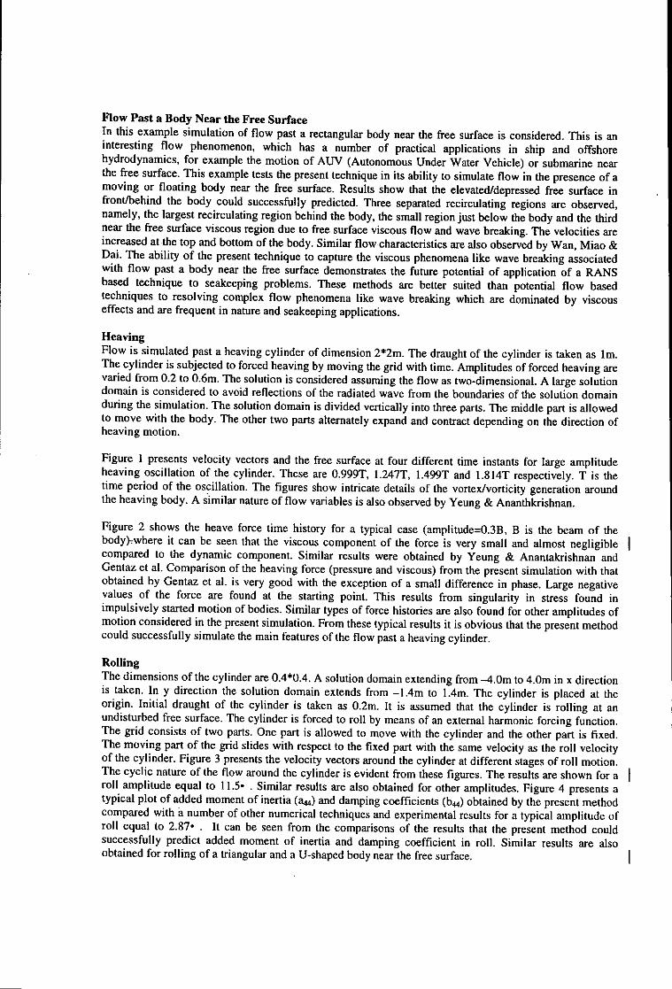
Flow Past a Body Near the Free SurfaceIn this example simulation of flow past a rectangular body near the free surface is considered. This is aninteresting flow phenomenon, which has a number of practical applications in ship and offshorehydrodynamics, for example the motion of AUV (Autonomous Under Water Vehicle) or submarine nearthe free surface. This example tests the present technique in its ability to simulate flow in the presence of amoving or floating body near the free surface. Results show that the elevated/depressed free surface infront/behind the body could successfully predicted. Three separated recirculating regions are observed,namely, the largest recirculating region behind the body, the small region just below the body and the thirdnear the free surface viscous region due to free surface viscous flow and wave breaking. The velocities areincreased at the top and bottom of the body. Similar flow characteristics are also observed by Wan, Miao &Dai. The ability of the present technique to capture the viscous phenomena like wave breaking associatedwith flow past a body near the free surface demonstrates the future potential of application of a RANSbased technique to seakeeping problems. These methods are better suited than potential flow basedtechniques to resolving complex flow phenomena like wave breaking which are dominated by viscouseffects and are frequent in nature and seakeeping applications.

HeavingFlow is simulated past a heaving cylinder of dimension 2*2m. The draught of the cylinder is taken as Im.The cylinder is subjected to forced heaving by moving the grid with time. Amplitudes of forced heaving arevaried from 0.2 to 0.6m. The solution is considered assuming the flow as two-dimensional. A large solutiondomain is considered to avoid reflections of the radiated wave from the boundaries of the solution domainduring the simulation. The solution domain is divided vertically into three parts. The middle part is allowedto move with the body. The other two parts alternately expand and contract depending on the direction ofheaving motion.

Figure 1 presents velocity vectors and the free surface at four different time instants for large amplitudeheaving oscillation of the cylinder. These are 0.999T, 1.247T, 1.499T and 1.814T respectively. T is thetime period of the oscillation. The figures show intricate details of the vortexivorticity generation aroundthe heaving body. A similar nature of flow variables is also observed by Yeung & Ananthkrishnan.

Figure 2 shows the heave force time history for a typical case (amplitude=0.3B, B is the beam of thebody)-where it can be seen that the viscous component of the force is very small and almost negligiblecompared to the dynamic component. Similar results were obtained by Yeung & Anantakrishnan andGentaz et al. Comparison of the heaving force (pressure and viscous) from the present simulation with thatobtained by Gentaz et al. is very good with the exception of a small difference in phase. Large negativevalues of the force are found at the starting point. This results from singularity in stress found inimpulsively started motion of bodies. Similar types of force histories are also found for other amplitudes ofmotion considered in the present simulation. From these typical results it is obvious that the present methodcould successfully simulate the main features of the flow past a heaving cylinder.

RollingThe dimensions of the cylinder are 0.4*0.4. A solution domain extending from -4.Om to 4.Om in x directionis taken. In y direction the solution domain extends from -l.4m to 1.4m. The cylinder is placed at theorigin. Initial draught of the cylinder is taken as 0.2m. It is assumed that the cylinder is rolling at anundisturbed free surface. The cylinder is forced to roll by means of an external harmonic forcing function.The grid consists of two parts. One part is allowed to move with the cylinder and the other part is fixed.The moving part of the grid slides with respect to the fixed part with the same velocity as the roll velocityof the cylinder. Figure 3 presents the velocity vectors around the cylinder at different stages of roll motion.The cyclic nature of the flow around the cylinder is evident from these figures. The results are shown for aroll amplitude equal to 11.5- . Similar results are also obtained for other amplitudes. Figure 4 presents atypical plot of added moment of inertia (a44) and damping coefficients (b44) obtained by the present methodcompared with a number of other numerical techniques and experimental results for a typical amplitude ofroll equal to 2.87° . It can be seen from the comparisons of the results that the present method couldsuccessfully predict added moment of inertia and damping coefficient in roll. Similar results are alsoobtained for rolling of a triangular and a U-shaped body near the free surface.

(a) t = 0.999T (b) t = 1.499T

© t 1.247T (d) t 1.814TFig. 1. Velocity Vectors & Free Surface (VOF=0.5) Plots for Heaving Cylinder

ConclusionIn this paper, results of application of a RANS-based technique in simulating a number of important flowphenomena are presented. The results show that the present technique could successfully simulate the keycharacteristics of the physical flow. In viscous flows, results produced are better than those obtained frominviscid techniques. This is particularly true for the roll added moment of inertia and damping coefficients.However, extensive validation tests including extension to practical 3-D hull forms are required beforecontemplating the application of the technique to real life problems.

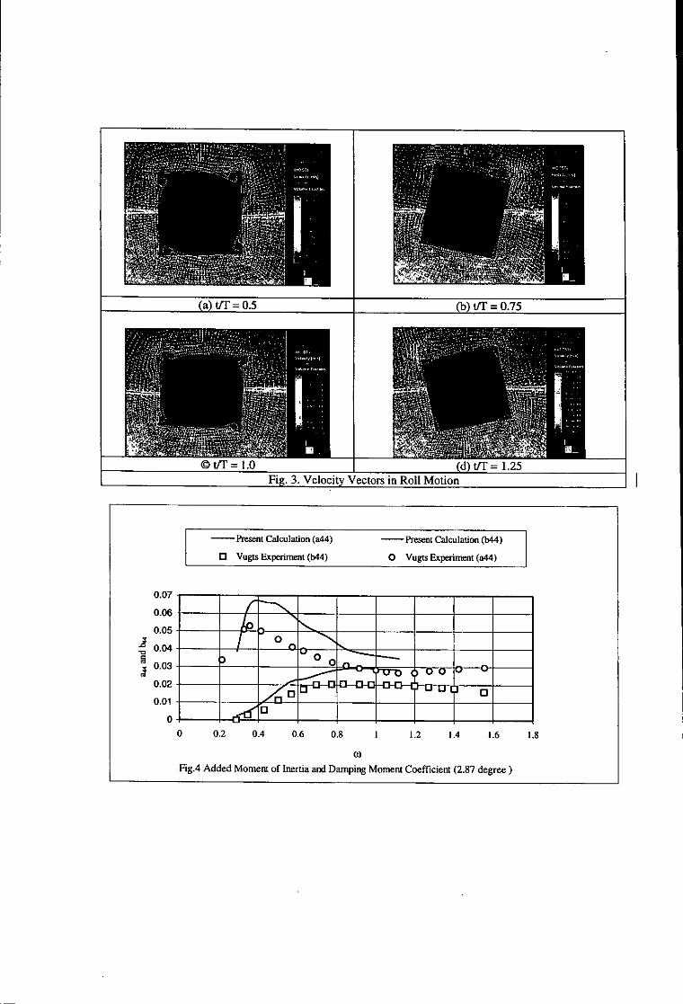
(a) UT=0.5 (b) tIt =0.75

-Present Calculation (au4) - Present Calculation (b44)

03 Vugts Experiment (W4) 0 Vugts Experiment (an4)

0.07 ___ ___

0.06 ____

0.05

0.04 -_ 0_ _ _

~0.03 - 3 0

0.02 - ___

0.01 ____l___

0 ___ ___

0 0.2 0.4 0.6 0.8 1 1.2 IA4 1.6 1.8

(0)

Fig.4 Added Moment of Inertia and Damping Moment Coefficient (2.87 degree)

Two Eulerian Approaches for Free-Surface Problems

Vladimir SHIGUNOV, Lars MUCKAB 3-13, Technical University Hamburg-Harburg, Hamburg, Germany

The paper presents two Eulerian methods for solving problems with moving contact bound-aries of fluids. The first method uses direct density advection to follow different fluids. It is basedon a Godunov-type approximation for flow variables and a preconditioned dual-time steppingscheme for pressure-velocity coupling. The second method represents a level set approach witha segregated solution scheme and a SIMPLE-type scheme for pressure-velocity connection. Bothmethods were tested on the example of a broken dam problem in a closed container.

1 Mathematical Model and Discretization Method

The problem concerned is about two contacting viscous incompressible fluids with different phys-ical properties. Variable density of the two-fluid system is used as a marker function for differentmaterials. Thus, the conservation of mass must be used:

Op(10-/+ v.(pv) = 0 (1)

together with conservation of momentum

t(pv) + (pv 0 v - P) pb (2)

and incompressibility constraint

V-,v = 0. (3)

Hier, p is the mass density, v is the velocity vector, b is the external body force acceleration,and P is the stress tensor, that reads

p = [vV + (Vv)T] - ZE, (4)

where p is the variable dynamic viscosity, p is the pressure, and 1 denotes the unit martix.The above formulation does not account for any interfacial effects, such as surface tension. It

can be taken into account by an appropriate treatment of the body-force term in (2). Formulation(1)-(3) allows a single-domain description of the two-fluid system and does not require anyboundary conditions at the interface due to the full conservative formulation and discretization.

The numerical approach for discretization of the governing equations is based on the conser-vative finite difference (finite volume) method in space and the second-order implicit trapezoidal

scheme in time. For storage of different flow variables, collocated grids are used in both methods.

2 Direct Density Advection Scheme

The system of flow equations (1)-(3) was preconditioned by adding pseudo-time derivatives eitherto all equations or only to the continuity equation. This approach alters the type of the inviscidpart of the incompressible Navier-Stokes equations from parabolic to totally hyperbolic andthus allows to apply established time-marshing methods from gas dynamics to incompressibleproblems. With this formulation, time-accurate solution is approached asymptotically at a givenphysical time level as a steady state solution in pseudo-time, which is called dual time-steppingprocedure.

With the dual time-stepping formulation, the left sides of all the equations (1) to (3) havethe same hyperbolic structure and can be solved in a fully coupled manner, which seems to bethe greatest advantage of the artificial compressibility-based formulations.

To advect a large density jump across the contact boundary, a discontinuous, Godunov-typeapproximation1 was used to represent flow variables. To reconstruct numerical inviscid fluxacross cell interfaces, approximate Riemann solver of Roe was used. To obtain cell face statesfor Riemann solver, high order upwind biased reconstruction schema of TVD (total variationdiminishing) type was applied.

Viscous fluxes were approximated with central differences in both methods.Physical time-stepping and dual time-stepping schemes are implicit. To solve resulting alge-

braic system, noniterative one-parametric implicit lower-upper approximate factorization schemewas developed. To accelerate convergence of dual time subiterations, local adaptive pseudo-timestep was used. CFL-number of pseudo-time iterations as well as the parameter of factorizationscheme and pseudo-compressibility parameter were adjasted in test calculations to obtain thebest convergence rate.

3 Level Set Scheme

Instead of using the mass conservation equation (1) direct, the level set approach represents thedensity as an one-argument function of the level-set function 4'(r, t), then Eq. (1) leads to thetransport equation for the level set function 0:

-t+ V. (Ov) = 0, (5)

Since the level set function has no strictly physical sence of a conserved variable, Eq. (5) wassolved in the non-conservative advection form:

a- + (vV)'= 0. (6)

To make possible the use of usual smooth reconstruction schemes, the exact density fieldin this solver was artificially smoothed in a transition zone of finite thickness near the contactboundary. To keep the thickness of this transition zone constant, PDF-based reinitializationprocedure was used.

Solution of the system (2), (3), and (6) at each physical time step was obtained in a segregatedmanner, so that one equation is solved in step. To eliminate decoupling and linearization errors,some number of outer iterations was carried out at every time step. Each equation was solvedby usual SIP oder CG-type iterative solvers.

Pressure-velocity coupling follows the idea of SIMPLE-type pressure-iteration procedures.To exclude pressure-velocity decoupling probleme connected with collocated grid arrangement,some additional correction terms were included in the pressure equation.

Since the density field is obtained with this solver indirect, through the level set function,we must expect both local and global mass conservation errors. Because of full conservativetreatment used for the momentum equation, the local mass conservation error leads to localinconsistency of momentum transport and then may deteriorate the solution process.

Instead of using non-conservative treatment of density in the momentum equations to solvethis problem, a simple correction of the present conservative scheme was developed by explicitinclusion of the mass conservation into discretized momentum equation. Resulting algorithmdoes not show any disturbances even for the overturning stage of motion.

'Godunov-type approximation implies evaluation of solution that is discontinuous across cell interfaces. This isachieved by solution of Riemanm problem for each cell interface with the following reconstruction of cell-averagedstates at the next time level. Godunov-tyjpe approximations were successfully applied in shock-capturing solversin gas dynamics and recently also for contact boundary problems.

2

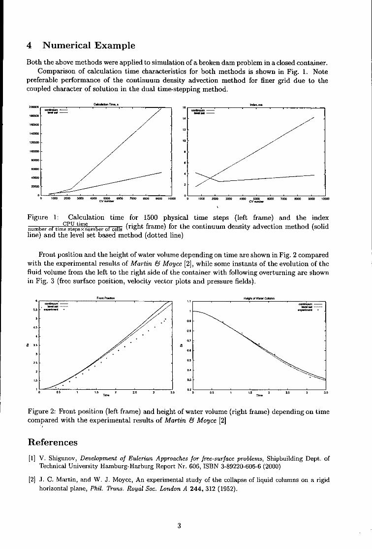
4 Numerical Example

Both the above methods were applied to simulation of a broken dam problem in a closed container.Comparison of calculation time characteristics for both methods is shown in Fig. 1. Note

preferable performance of the continuum density advection method for finer grid due to thecoupled character of solution in the dual time-stepping method.

2./

--- -/--°

m t2

Figure 1: Calculation time for 1500 physical time steps (left firame) and the indexnumber of time tpxubrocel (right frame) for the continuum density advection method (solid

line) and the level set based method (dotted line)

Front position and the height of water volume depending on time are shown in Fig. 2 comparedwith the experimental results of Martin & Moyce [2], while some instants of the evolution of thefluid volume from the left to the right side of the container with following overturning are shownin Fig. 3 (free surface position, velocity vector plots and pressure fields).

/ 4Z.. . -.A- _

- .- "

/ 2, -

5o

4ý5

2 0,

Figure 2: Front position (left frame) and height of water volume (right frame) depending on timecompared with the experimental results of Martin & Moyce [2]

References

[1] V. Shigunov, Development of Eulerian Approaches for free-surface problems, Shipbuilding Dept. ofTechnical University Hamburg-Harburg Report Nr. 606, ISBN 3-89220-606-6 (2000)

[2l J. C. Martin, and W. J. Moyce, An experimental study of the collapse of liquid columns on a rigidhorizontal plane, Phil. Tioans. Royal Soc. London A 244,p312 (1952).

FrailPvJ3

... ... .. ... .- -- -- _ --- -- --- - I.. ... ... -- --- --- --- ...........--- -- -- -- -- -- -- -- -- --- -- -- -- -- -- -- -- -- :- -.::

. . . . . . .. .. -- -- -- - - --- -- -- -- - - - - --- - --- -- - - - - - -- -- -- i--m- - . 2-2.7- -- -- -- -- -- -- - - - -- - -- -- -- -- -- -- -- - - - - - - -- -- -- N----- --

-- - - -- - -- - -- - --- - -- - -- - -- -- - --- -- - - -- -- - --- - -- - -0 44

- -- - -- --- --- -- - - ---- -- -- --- --- -

-------- -------tim - -.0 -I

-'o 8.0 , : :--------n =: : -- -- - ---- - - - - -. . . . . . . . . . . .

72.7

Figure.... 3:V lct.eto .ilsad. dniycnor.lt.ihcrrsodn.rssr itiution obtained wit thefistmeho

............ ....

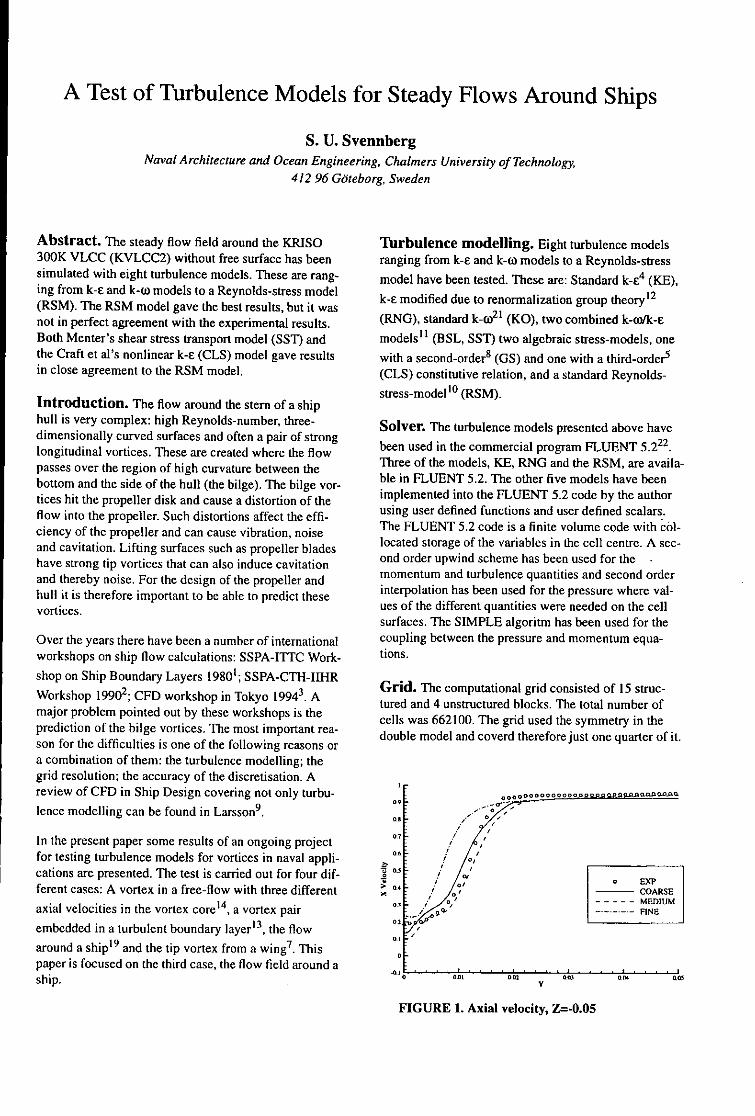
A Test of Turbulence Models for Steady Flows Around Ships

S. U. SvennbergNaval Architecture and Ocean Engineering, Chalmers University of Technology,

412 96 Gdteborg, Sweden

Abstract. The steady flow field around the KRISO TLrbulence modelling. Eight turbulence models300K VLCC (KVLCC2) without free surface has been ranging from k-e and k-(o models to a Reynolds-stresssimulated with eight turbulence models. These are rang- model have been tested. These are: Standard k-04 (KE),ing from k-e and k-w models to a Reynolds-stress model k-s modified due to renormalization group theory 12

(RSM). The RSM model gave the best results, but it wasnot in perfect agreement with the experimental results. (RNG), standard k-o 21 (KO), two combined k-og/k-cBoth Menter's shear stress transport model (SST) and models"1 (BSL, SST) two algebraic stress-models, onethe Craft et al's nonlinear k-s (CLS) model gave results with a second-order8 (GS) and one with a third-order 5

in close agreement to the RSM model. (CLS) constitutive relation, and a standard Reynolds-stress-model1 ° (RSM).

Introduction. The flow around the stern of a ship

hull is very complex: high Reynolds-number, three- Solver. The turbulence models presented above havedimensionally curved surfaces and often a pair of strong 22longitudinal vortices. These are created where the flow been used in the commercial program FLUENT 5.2passes over the region of high curvature between the Three of the models, KE, RNG and the RSM, are availa-

bottom and the side of the hull (the bilge). The bilge vor- ble in FLUENT 5.2. The other five models have beentices hit the propeller disk and cause a distortion of the implemented into the FLUENT 5.2 code by the authorflow into the propeller. Such distortions affect the effi- using user defined functions and user defined scalars.ciency of the propeller and can cause vibration, noise The FLUENT 5.2 code is a finite volume code with col-and cavitation. Lifting surfaces such as propeller blades located storage of the variables in the cell centre. A sec-have strong tip vortices that can also induce cavitation ond order upwind scheme has been used for theand thereby noise. For the design of the propeller and momentum and turbulence quantities and second orderhull it is therefore important to be able to predict these interpolation has been used for the pressure where val-vortices. ues of the different quantities were needed on the cell

surfaces. The SIMPLE algoritm has been used for theOver the years there have been a number of international coupling between the pressure and momentum equa-workshops on ship flow calculations: SSPA-ITTC Work- tions.shop on Ship Boundary Layers 19801; SSPA-CTH-IIHR

Workhop19W CF woksho inToko 1943Grid. The computational grid consisted of 15 struc-k .A tured and 4 unstructured blocks. The total number of

major problem pointed out by these workshops is the cells was 662100. The grid used the symmetry in theprediction of the bilge vortices. The most important rea- double model and coverd therefore just one quarter of it.son for the difficulties is one of the following reasons ora combination of them: the turbulence modelling; thegrid resolution; the accuracy of the discretisation. Areview of CFD in Ship Design covering not only turbu- ................lence modelling can be found in Larsson9.

In the present paper some results of an ongoing projectfor testing turbulence models for vortices in naval appli- ,cations are presented. The test is carded out for four dif-ferent cases: A vortex in a free-flow with three different >' 04

axial velocities in the vortex core14, a vortex pair 03 .-.. FNE

embedded in a turbulent boundary layer' 3 , the flow o,around a ship 19 and the tip vortex from a wing 7. This t -paper is focused on the third case, the flow field around a 4'0ship. 000a

FIGURE 1. Axial velocity, Z=-0.05

From the figures its obvious that no one of the modelsmanages to predict the flow field in the propeller plane

.15,' 7 perfectly, but all models show that there are bilge vorti-ces present. The RSM model predicts the flow field in

0,)5 , 'closest agreement with the experiments, but both theS. . ExP SST model with its limit on the turbulent viscosity and

-- COARSESF MEDIUM the CLS model with its nonlinear constitutive relation.1 o give results close to the RSM model.

o ModelTable 1: Resistance coefficients

Model Cp 103 CF* 10' CT* 10' k

0.0 001 o0 0e 0.4 EXP 0.680 3.450 4.130

FIGURE 2. turbulent kinetic energy, Z=-0.05 KE 0.855 3.764 4.619 0.3390

The form of the grid was a quarter of a cylinder with half RNG 0.873 3.679 4.552 0.3195spheres at the ends. It had a length of two and a width of KO 0.915 3.681 4.596 0.3324half a ship length. A grid refinement test including twocoarser grids has been done. The flow structure in the BSL 0.925 3.555 4.480 0.2989propeller plane changes considerably between the differ-ent grids. There is no monotonic convergence. This canbe seen in Figure I and Figure 2 where the axial velocity GS 1.413 5.382 6.794 0.9696and turbulent kinetic energy are plotted along the Z=--0.05 line for the three different grids. The verification CLS 1.158 4.427 5.586 0.6192methodology suggested by Stern et a115 needs monot- RSM 1.035 4.383 5.418 0.5707onic convergence for a verification using only threegrids. The coarsest grid is too coarse so its no idea tomake a coarser grid, so a finer grid will be created. Deng and Visonneau 6 have showed that the wall reflec-

tion term in the present RSM model reduces the second-Results and discussion. Calculated resistance ary velocities close to the wall. This reduction affects thecoefficients are presented in Table I below. The experi- strength of the bilge vortices and might explain the over-mental data (EXP) comes from the towing-tank test 20 prediction of the resistance.

while all the flowdata in the present paper come fromtest 9. he vscos drg ceffiien CF(FO) Deng and Visonneau6 also shoved that the assumption ofwind-tunnel test 19 . The viscous drag coefficient CF (CF0) local equilibrium between production and dissipation offor the EXP data is calculated using the ITTC-57 line turbulence is not valid at the propeller plane of a similarand the pressure coefficient Cp is the residuary resistance flow. Nonlinear algebraic RSM models such as the GSfrom the towing tank experiment, i.e. both the wave and and the CLS models are based on an asumption of localpressure drag is included in this figure. The form factor k equilibrium. These models should therefore not beis calculated using k = CT/CFO - 1. The total resistance expected to give accurate results since this condition isis overpredicted by all the tested models. The SST model not fullfilled at the propeller plane.that predicts the lowest drag has a limit on the turbulent The OS model gave more pronounced hook shape in theviscosity close to the wall. Low viscosity close to the iso contour e aveloct thante Kmodel thawall gives lover viscous drag and the SST model under- is otus of the axial velocity than the KE model thatpredicts the viscous drag. it is based on, but less than the CLS model. In fact it is

quite close to the hook shape predicted with the KO

The flow field in the propeller plane computed with model, and it is therefore not plotted in this short paper.some of the models can be found in Figure 4 - Figure 8 The CLS model is also based on the KE model in thisand the experimental data from the wind-tunnel test 19 test. Comparing the results of the KE model with theare plotted in Figure 3. Contours of the axial velocity are results of the CSL model it can be seen that the aniso-plotted in the left part of the figures and vectors of the tropic terms in the constitutive relation are of greatsecondary velocity components are plotted in the right importance even though the equilibrium condition is notpart of the figures, only every third vector is plotted to satisfied in this flow. The nonlinear terms reduce the pro-make the figures readable. The velocities are normalised duction of turbulent energy in the vortex.by the undisturbed free stream velocity and the referencevector equals a velocity of magnitude one.

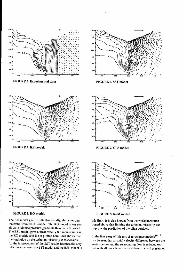
--. \i RX\

FIGURE 3. Experimental data FIGURE 6. SST model0.96

.... .0 W..

FIGURE 4. KE model. FIGURE 7. CLS model

NNN'N NNN-.401

00 -OW\FIGURE 5. KO model. FIGURE 8. RSM model

The KO model gave results that are slightly better than this limit. It is also known from the workshops men-the result from the KE model. The KO model is less sen- tioned above that limiting the turbulent viscosity cansitive to adverse pressure gradients than the KE model. improve the prediction of the bilge vortices.The BSL model gave almost exactly the same results asthe KO model, so it is not plotted here. This shows that In the first parts of this test of turbulence models 16 ,17 itthe limitation on the turbulent viscosity is responsible can be seen that an axial velocity difference between thefor the improvement of the SST results because the only vortex centre and the surrounding flow is reduced toodifference between the SST model and the BSL model is fast with all models no matter if there is a wall present or

not. This can explain why the hook shape in the axial Referencesvelocity contours is less pronounced in the computationsthan in the experiment while the vortex strength and [1] Proceedings, "SSPA-ITTC Workshop on Ship Boundary Layers"

(1980), Ed. L. Larsson, SSPA Report No. 90, 1980, Gtteborg,position seems to be of the right size, as can be seen in Sweden.Figure 9 below. [2] Proceedings, "1990 SSPA-CTH-IIHR Workshop on Ship Viscous

Flow" (1990), Eds. L. Larsson, V. C. Patel and G. Dyne,Research Report No. 2. Flowtech International AB, 1991 Gbte-

00 borg. Sweden.

[3] Proceedings, "CFD Workshop Tokyo 1994", (1994) Ed. Y.Kodanm, Ship Research Institute, Tokyo, Japan

S[4] Chen H. C. and Pat V. C., AIAA Journal, June 1988, vol. 26,No. 6, pp. 641-648

[5] Craft T. J., Launder B. E. and Suga K., Int. J. Heat and Fluid0• /o XP Flow, vol. 17, no. 2, April 1996

--- -. .--- T [6] Deng G. B. and Visonneau M., Seventh International Conference- ......-.. SST51

-........ CLS on Numerical Ship Hydrodynamics, July 1999, Nantes, France.2, _/ SM [7] Froman D., Dugue C., Pauchet A., Cerruti P., Briancon-Marjolet

L., Ninetenth Symposium on Naval Hydrodynamics, 1992, Seoul,Korea

v 0o o ow [8] Gatski T. B. and Speziale C. G., Journal of Fluid Mechanics, vol.254, 1993. pp. 59-78

FIGURE 9. Vertical velocity along a horizontal

line trough the vortex centre [9] Larsson L., Ship Technology Research, July 1997, vol. 44, no. 3,pp. 135-154.

All the different models predict not just the bilge vortex [10] Launder B. E. and Shima N., AIAA Journal, 1989, vol. 27, No.

they also predict a second smaller vortex. The KE, RNG, 10, pp. 1319-1325

GS and CLS models predict a weaker secondary vortex [1il Menter F. R, AIAA Journal, August 1994, vol. 32, No. 8.than the other models. In the experimental data this vor- pp. 1598-1605tex is just seen as a small disturbance in Figure 3 but the [12] Orzag S. A., Yakhot V., Flannery W. S., Boysan F, Choudhuryexperimental data is not completely symmetric and this D., Mamzevsky J. and Patel B., Near wall Turbulent Flows, page

vortex is more pronounced on the other side of the cen- 1031. Elsevier Science Publishers B. V., 1993

terline. The data on the other side of the centerline are [13] Pauley W. R. and Eaton J. K., AIAA Journal, 1988 vol. 26, No. 7,not plotted in the figure to make the iso-contours more pp. 816-823

visible. The propeller hub is cut off straight in the exper- [14] Phillips W. R. C. and Graham J.A.H., Journal of Fluid Mechanics,iments while it is rounded in the calculations. This 1984, vol. 147, pp. 353-371rounding comes from the surface mesh provided by the [15] Stem F., Wilson R. V., Coleman H. W., Paterson E., G., Iowaorganisers of the Gothenburg 2000 workshop. This mesh Institute of Hydraulic Research, IIHR Report No. 407, Septemberis used as surface description in the computations. The 1999round tip can strengthen such vortices. [161 Svennberg S. U., "A Test of Turbulence Models for a Vortex in a

Free-Stream", Licentiate Thesis, Department of Naval Architec-A more complete presentation and discussion of the ture and Ocean Engineering, Chalmers University of Technology,

results in this test will soon be publishedl 8 . Gdteborg Sweden, CHA/NAV/R-96/0047

[17] Svennberg S. U., "A Test of Turbulence Models for a Vortex PairEmbedded in a Turbulent Boundary Layer", Department of NavalConclusions. Eight turbulence models have been Architecture and Ocean Engineering, Chalmers University of

tested on the steady flow around the KRISO 300K Technology, Gbteborg Sweden, CHA/NAV/R-98/0055VLCC (KVLCC2) without free water surface. It is a 118] Svennberg S. U."A Test of Turbulence Models for Bilge Vorti-challenging task to predict the complex flow field at the ces", Dapartment of Naval Architecture and Ocean Engineering,stern of a ship. No one of the tested turbulence models Chalmers University of Technology, G6teborg Sweden, CHA/manages to reproduce the flow field completely. Simple NAV/R-98/0056

modifications such as the limitation of the turbulent vis- [19] Van S.H., Kim W.J., Kim H. R., and Lee SJ. "Wind Tunel Test oncosity in the SST model can give considerable improve- Flow Characteristics of KRISO 300K VLCC double model", Pro-ments of the results. Even thoug the RSM model gives ceedings of Japan-Korea Joint Workshop on Marine Hydrody-

results in closest agreement with the experimental data namics (JAKOM99), Fukuoka, Japan.

and with a pronounced hook shape in the iso-contours of [20] Van, S.H., Kim, W.J., Yim, G.T., Kim, D.H., and Lee, CJ., 1998,

the axial velocity, there is considerably more to be done Proceedings 3rd Osaka Colloquium on Advanced CFD Applica-tions to Ship Flow and Hull Form Design, Osaka, Japanto reach a perfect simulation result.

[21] Wilcox D.C., "Turbulence Modelling for CFD" DCW Industries,1993, ISBN 0-9636051-0-0

[22] www.fluent.com

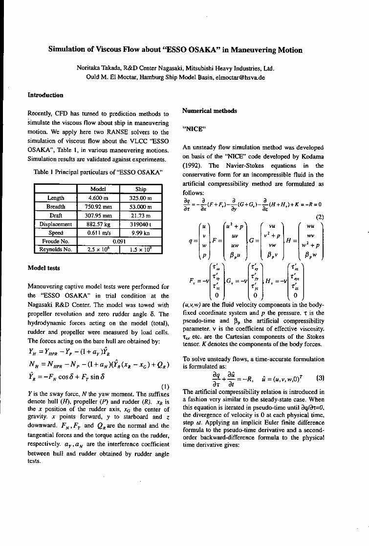
Simulation of Viscous Flow about "ESSO OSAKA" in Maneuvering Motion

Noritaka Takada, R&D Center Nagasaki, Mitsubishi Heavy Industries, Ltd.Ould M. El Moctar, Hamburg Ship Model Basin, elmoctar@hsva.de

Introduction

Recently, CRD has turned to prediction methods to Numerical methods

simulate the viscous flow about ship in maneuveringmotion. We apply here two RANSE solvers to the "NICE"simulation of viscous flow about the VLCC "ESSOOSAKA", Table 1, in various maneuvering motions. An unsteady flow simulation method was developed

Simulation results are validated against experiments. on basis of the "NICE" code developed by Kodama(1992). The Navier-Stokes equations in the

Table I Principal particulars of "ESSO OSAKA" conservative form for an incompressible fluid in theartificial compressibility method are formulated as

Model Ship follows:Length 4.600mi 325.00Gm a a a a)Length~ ~ =.0 _ 32.0 mq=f-(F+F,)- (G+G,)-T--(H+H,)+K =-R=0Breadth 750.92 mm 53.000m air ax ii; )-z

Draft 307.95 mm 21.73 m (2)Displacement 882.57 kg 319040 t u + p vui wu

Speed 0.611,m/s 9.99 kn u_/jF_/ uov G 'O-- H-Froude No. 0.091 q-f1F [ = IV H - +

Reynolds No. 2.5 x 106 1.5 x I0V J UW i JpW

Model tests T ýT

Maneuvering captive model tests were performed for F = T'the "ESSO OSAKA" in trial condition at the 0 0 01Nagasaki R&D Center. The model was towed with (u,vw) are the fluid velocity components in the body-propeller revolution and zero rudder angle 8. The fixed coordinate system and p the pressure. t is thehydrodynamic forces acting on the model (total), pseudo-time and Op the artificial compressibility

rudder and propeller were measured by load cells, parameter. v is the coefficient of effective viscosity.,t. etc. are the Cartesian components of the StokesThe forces acting on the bare hull are obtained by: tensor. K denotes the components of the body forces.

Y,, = r,,pR - Yp - (1 + aY )YRTo solve unsteady flows, a time-accurate formulation

NU1 =NpR -Np -- (l+aN)(YR(xR - X)+QR) is formulated as:

YR =-FNcos8 + FTsine 3q +-=-R, 12=(u,v,w,O)" (3)(1) ar 8t

Y is the sway force, N the yaw moment. The suffixes The artificial compressibility relation is introduced indenote hull (H), propeller (P) and rudder (R). xR is a fashion very similar to the steady-state case. Whenthe x position of the rudder axis, xG the center of this equation is iterated in pseudo-time until aq/at=0,gravity. x points forward, y to starboard and z the divergence of velocity is 0 at each physical time,downward. ~ FNF and Q are the normal and the step At. Applying an implicit Euler finite differencea R formula to the pseudo-time derivative and a second-tangential forces and the torque acting on the rudder, order backward-difference formula to the physicalrespectively. ay,a N are the interference coefficient time derivative gives:between hull and rudder obtained by rudder angletests.

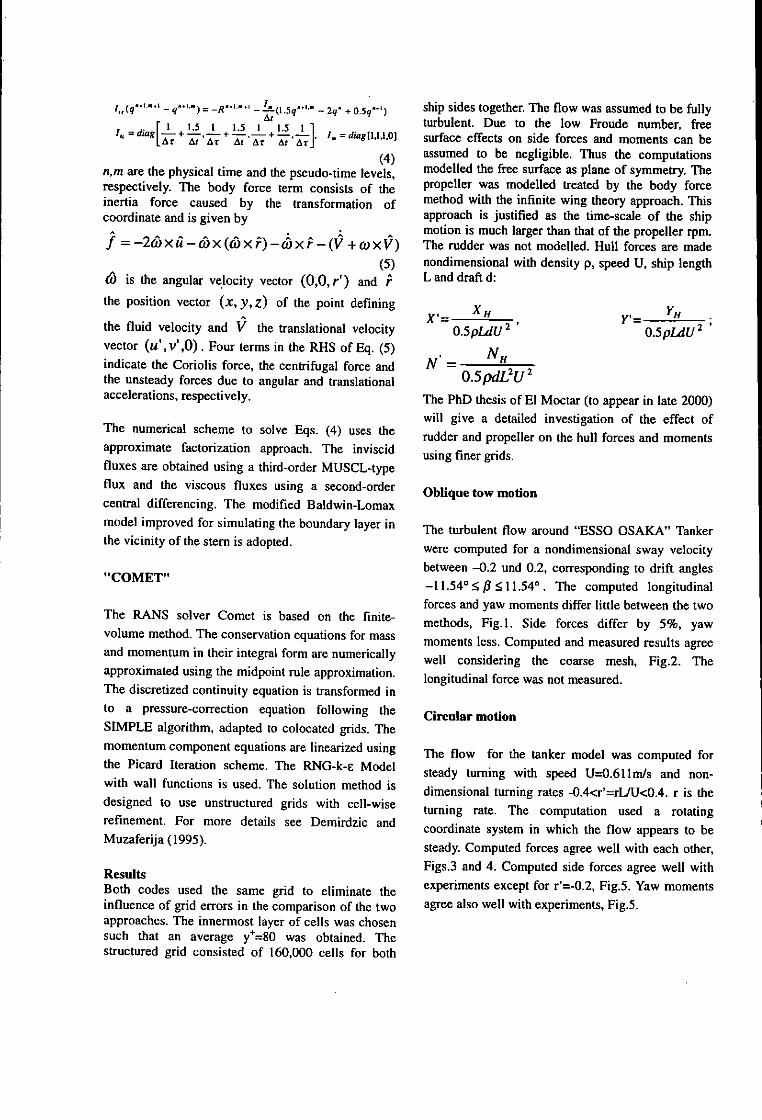
i qaql)-R-1-' -t(1.5q- "' - 2 q" +0.5q-') ship sides together. The flow was assumed to be fullyAt1,15g | 1L 5 ± 1 _l turbulent. Due to the low Froude number, free

diag A 1.5 A1.• .5:ArA A .]-diag[l'l.I.O] surface effects on side forces and moments can beITT AT ,z 1tT AT At Ad""

(4) assumed to be negligible. Thus the computationsn,m are the physical time and the pseudo-time levels, modelled the free surface as plane of symmetry. Therespectively. The body force term consists of the propeller was modelled treated by the body forceinertia force caused by the transformation of method with the infinite wing theory approach. Thiscoordinate and is given by approach is justified as the time-scale of the ship

motion is much larger than that of the propeller rpm.f =-2bxa-c- x(cbxP)-oaxb-(.V+wxov) The rudder was not modelled. Hull forces are made(5) nondimensional with density p, speed U, ship length

0) is the angular velocity vector (0,0,r') and r Land draft d:the position vector (x, y, z) of the point defining X.= XH Y F -

the fluid velocity and V the translational velocity 0.5pLdU 2 0.5pLdU 2 'vector (u',v',0). Four terms in the RHS of Eq. (5) NHindicate the Coriolis force, the centrifugal force and N =-the unsteady forces due to angular and translational 0.5pdL2U 2

accelerations, respectively. The PhD thesis of El Moctar (to appear in late 2000)will give a detailed investigation of the effect of

The numerical scheme to solve Eqs. (4) uses the rudder and propeller on the hull forces and momentsapproximate factorization approach. The inviscid using finer grids.fluxes are obtained using a third-order MUSCL-typeflux and the viscous fluxes using a second-order Oblique tow motioncentral differencing. The modified Baldwin-Lomaxmodel improved for simulating the boundary layer in The turbulent flow around "ESSO OSAKA" Tankerthe vicinity of the stem is adopted. were computed for a nondimensional sway velocity

between -0.2 und 0.2, corresponding to drift angles"COMET" -11.540 < 5 511.54'. The computed longitudinalforces and yaw moments differ little between the two

The RANS solver Comet is based on the finite- methods, Fig.l. Side forces differ by 5%, yawvolume method. The conservation equations for mass moments less. Computed and measured results agreeand momentum in their integral form are numerically well considering the coarse mesh, Fig.2. Theapproximated using the midpoint rule approximation. longitudinal force was not measured.The discretized continuity equation is transformed into a pressure-correction equation following the Circular motionSIMPLE algorithm, adapted to colocated grids. Themomentum component equations are linearized using The flow for the tanker model was computed forthe Picard Iteration scheme. The RNG-k-e Model steady turning with speed U--0.611m/s and non-with wall functions is used. The solution method is dimensional turning rates -0.4<r'=rLIU<0.4. r is thedesigned to use unstructured grids with cell-wise turning rate. The computation used a rotatingrefinement. For more details see Demirdzic and coordinate system in which the flow appears to beMuzaferija (1995). steady. Computed forces agree well with each other,

Results Figs.3 and 4. Computed side forces agree well withBoth codes used the same grid to eliminate the experiments except for r'=-0.2, Fig.5. Yaw momentsinfluence of grid errors in the comparison of the two agree also well with experiments, Fig.5.approaches. The innermost layer of cells was chosensuch that an average y`=80 was obtained. Thestructured grid consisted of 160,000 cells for both

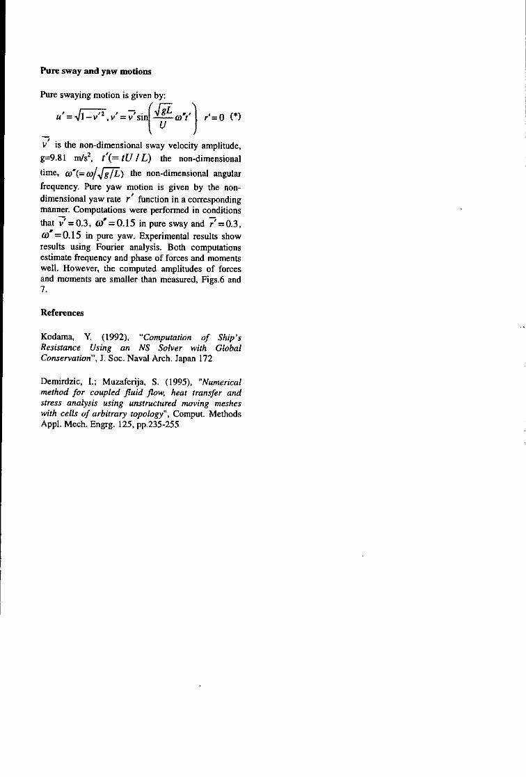
Pure sway and yaw motions

Pure swaying motion is given by:

u'=V-v`,'=vsin - &':LO) r'= 0(*(I U I

V is the non-dimensional sway velocity amplitude,g=9.81 m/s2, t'(= tU IL) the non-dimensional

time, d'(=aw/47gE) the non-dimensional angularfrequency. Pure yaw motion is given by the non-dimensional yaw rate r' function in a correspondingmanner. Computations were performed in conditionsthat v=0.3, aw'=0.15 in pure sway and r=0.3,0) = 0.15 in pure yaw. Experimental results showresults using Fourier analysis. Both computationsestimate frequency and phase of forces and momentswell. However, the computed amplitudes of forcesand moments are smaller than measured, Figs.6 and7.

References

Kodama, Y. (1992), "Computation of Ship'sResistance Using an NS Solver with GlobalConservation", J. Soc. Naval Arch. Japan 172

Demirdzic, I.; Muzaferija, S. (1995), "Numericalmethod for coupled fluid flow, heat transfer andstress analysis using unstructured moving mesheswith cells of arbitrary topology", Comput. MethodsAppl. Mech. Engrg. 125, pp. 2 35 -2 5 5

92.

...... ..... .. .. ..... 2.2 *oM t 0 -I

I ,NICE ---7 I E x - 2 .- i .. ............-. ..... ... ...Comet --

2~~~~...... -- = i = tn r~i ,!~ . - ------- I--

1.40 ... p0..-j. . ...

4 . ..... ..... ......... .ih u Pr.... ..I..... ....Co.2p .t Po -2. . .... .......N.C ---x -.... ..

....... ~ ~ ~ ~ ~ ~~ Co e .-. e -...... ............ .. ..........z ...........5.-

1 0 2 1

1-0.-V-

Fi.1:Cmue ocsadmoments, (hpnoblique flow)mto without Propeller

0o 5................ Cam w.h u P.C mproho tPr p- --- -

4 Conip with Prop. oa

102 W

0 0.1~' 22 y3 0.4 ..... 4.....0 0 10 0 04 .

rQ r,

Fig. 4: Cmue a oetsi ncrua i Measured and NICE-computed forces andFi.3Coptdsefrchpinicua

moet olqefo) motion without Propeller. moet(cruamtin

01 51

0m1 1 1 1

NIC0 ----- 4Cm.wt rp

0~~5.* o

Fig.6: Te tie hstor of he say orceFig.7: he tme hstor ofthe.way.orcand... ya moment. in pure. swyn moton.nd.aw.om..i.pue.ywin.moio

Adaptive grid flow solutions around a Mariner hull at drift

Turnock, S.R., Wright A.M., Pattenden, R., Pemberton R.School of Engineering Sciences, Ship Science, University of Southampton, Southampton. U.K.

Tel No: 44 (0)23 80592488 Fax No: 44 (0)23 80593299 Email: steve@ship.soton.ac.uk

IntroductionFlow solutions around realistic ship hull forms require a high quality mesh, which has adequate resolution in areas ofinterest and yet minimises the total computational effort. In the case of a ship at an effective angle of drift, for exampleduring a low speed manoeuvre, the hull behaves like an extremely low-aspect ratio wing and the magnitude of the sideforce is controlled by the rotational flow generated over the keel. In this case it is not possible a priori to identify wherethe vortical flow exists and hence where high grid resolution is required. This work examines for the Mariner hull[l] atdrift how the flow code ERIC[2], currently under development at Southampton, is used to capture correctly the flow andhence calculate the side force.

A conventional multi-block structured mesh is still the most common approach for sub-dividing the fluid domain intodiscrete finite volumes. A hyper-cube approach allows the addition of smaller blocks at suitable locations away fromthe hull surface[3]. However, this may require a progressive level of solutions at each stage - solving a coarse mesh,generating a new finer block structure and then resolving. The approach taken in this work is to operate on individualfinite volume cells through a process of sub-division during solution convergence. The control of this sub-division processis determined by the local pressure gradient, as well as a quantified measure of geometrical grid quality.

Flow SolverERIC (EuleR Incompressible Code) uses artifical compressibility [4] within a flux vector splitting framework upon a nodecentred Euler solver. Unstructured data allows the use of arbitrary polyhedrals and hence no restrictions are placed onmesh adaption. An explicit Runge-Kutta method is used to march the solution to steady state.

The basic format of artificial compressibility replaces the density term in the mass conservation equation with apressure term which allows evolution through time. During time marching this set of equations will have no physicalmeaning but in steady state the time derivatives tend to zero and satisfy the standard Euler equations. The format of thegoverning equations, adapted for artificial compressiblity, are -

aU +0OF 0G + OH>at a x Oy 8z/p- C2o( +T ; o l

U= v 0 0 010100 "= u2+uv I G= v2+p Ivw

w 0 0 0l 1 UW Vto 2s + p

0 can be viewed as a preconditioning matrix, with c being the artificial speed of sound. From this an analogy with theequation of state for compressible flow can be drawn -

p = ep, (2)

Thus pa is an artificial density, hence the term artificial compressibility.The initial selection of a value for the artificial speed of sound, c, is that derived by Farmer et al (1994) -

o2 = MAX (K(u 2 + v2 + W2), CiN) (3)

where K is a constant.The flux terms of the conservative form of the Euler equations (1) can be split according to the direction of the

characteristics via the directionalised Jacobian. Taking the one dimensional problem as a case study, if F+ is discretisedwith a backward difference scheme and F- discretised with a forward difference then the concept of the upwind scheme

will be realised. The subscript i defines the discrete spatial position while the superscript n defines the timestep. Thisformulation results in

U!, Ot -F*u?= ,+(F -F?½Ix +Fi t-3

where F? F.+L+F IAIU'+1 2- (4)

This scheme is Il t order accurate in both time and space. A higher order scheme (e.g. MUSCL) has not beenimplemented so far due to the unstructured nature of the spatial grid and the resultant unstable nature of higher orderschemes.

The calculation of the individual split eigenvalues is accomplished in the same manner as that by [5]. -

A± =A ± vr C (5)

2The E is added because of the lack of continual differentiablity at zeros of the eigenvalue (i.e. sonic and stagnation

points). It should be noted that for the case of artificial compressibility only stagnation points are of interest due to theflow being sub-pseudosonic at all times.

Thus we have a first order scheme where the conservative vector and flux vector states at each of the nodes surroundinga face are combined to produce the flux through the face. This is purely one dimensional, but can be expanded into threedimensions by the adoption of the generalised Jacobian matrix K and the summation of the flux through all surroundingfaces, such that the flux integral, C, is defined as

At no.facea

(U) --V F.Area0 (6)

This generalised nature of the flux and conservative variables vectors allows the use of arbitrary polyhedral controlvolumes. The explicit time marching scheme is a four stage Runge-Kutta Method.

Adaption Control

A statistical analysis of all the cells is conducted based on pressure gradient and those outwith set limits (typically twostandard deviations from the mean) are either split or fused. Once an individual cell is designated to be split the process iscarried out by first defining the direction of maximum pressure gradient. A cutting plane can then be defined through thevolumetric centre of the cell. All the cell faces which are cut by this plane are split along the dividing line and two newcells are formed either side of the cutting plane. The cell inter-connections of the parent are kept through the use of a treestructure. Fusion of cells can then be carried out simply on all but the initial coarse mesh.

It is possible to measure the geometric properties of a finite volume cell and determine how they relate to the localsolution quality. The results of such an analysis show that of the primitive variables, solution accuracy is most sensitive topressure gradients. However, geometrical properties have a marked effect upon solution accuracy and convergence, withskew being of greatest importance [6]. Figure 1 shows the results of such studies. Mesh quality is maintained through thesolution cycle by periodic readjustment of the position the control nodes defining the position of faces between controlvolumes. A least squares process is used to adjust the control nodes to minimise facial skew, deviation from planarity, andcontrol aspect ratio.

An initial coarse mesh is generated using a block structured mesh generator, Fleximesh[7]. For maximum effectivenessthe number of blocks should be kept to a minimum. On commencement of the iterative solution process a periodicmesh refinement process is carried out. This is controlled by a given drop in the level of average residuals. Progressiverefinement is carried out until a fixed number of finite volume of cells are in existence. Once this level has been achievedcoarser elements are fused if further refinement is required.

Mariner Hull Test Case

The geometric shape of the hull previously used for surface panel calculations [8] of sideforce was used as an input intothe block structured mesh generation program Fleximesh. An initial structure of 16 blocks was used. Figure 2 shows thedouble hull surface representation of the Mariner form.

Results will be presented for an angle of drift of 7.50, with particular emphasis upon the increased resolution of thevortical flow for a constant number of control volumes. In addition, experimental results from the truncated hull based onthe Mariner tested in the 3.5m x 2.5m wind tunnel [9] will be used for comparative purposes.

2

6*'

5 .- ' " .... ' ... ... ..... . .... .

4.

Coefficient of,-propovtionality 3 -

Hump. l8 x S. 30%Hump, 18 x 5, 45%

Hump, 58 x15, 30%

... Hupe8 x15,45 Mesh family

0' Hump, 118x 30,30%Skew ft ra . l NACA 0012, 343 x 25, 30%of alnorMalDVnfo

Geomettical property pwwy

Figure 1: Relative importance of geometrical properties for mesh distortions

F.-M

Figure 2: Mariner Double hull

3

References[1] V.L. Russo and E.K. Sullivan. Design of the mariner-type ship. Transactions of SNAME, 61, 1953.

[2] A. M. Wright. "Automated adaptation of spatial grids forflow solutions around marine bodies of complex geometry".PhD thesis, to be submitted University of Southampton, 2000.

[3] J. F. Thompson, B. K. Soni, and N. P. Weatherill, editors. "Handbook of Grid Generation". CRC Press, 1999. ISBN0-8493-2687-7.

[4] A. J. Chorin. "A numerical method for solving incompressible viscous flow problems". Journal of ComputationalPhysics, 2:12-26, 1967.

[5] J. L. Steger and R. F. Warming. "Flux vector splitting of the inviscid Gasdynamic equations with applications to finitedifference methods". Journal of Computational Physics, 40(2):263-293, April 1981.

[6] A. M. Wright and S. R. Turmock. "Efficient multi-level adaptation methods for unstructured polyhedral computationalmeshes". Ship Science Report 109, Department of Ship Science, University of Southampton, 1999.

[7] N. C. Rycroft and S. R. Turnock. "3-D Multiblock Grid Generator; FLEXIMESH". Ship Science Report 101,Department of Ship Science, University of Southampton, 1997.

[8] S.R. Tumock, Molland, A.F. The effects of shallow water and channel walls on the low-speed manoeuvring per-formance of a mariner hull with rudder. In Proc. of International symposium and workshop on forces acting on amanoeuvring vessel, MAN'98, Val de Reuil, France, 1998.

[9] AF. Molland and S.R. Turnock. Wind tunnel tests on the effect of a ship hull on rudder-propeller interaction atdifferent angles of drift. Ship Science Report 76, University of Southampton, 1995.

4

SELF - PROPULSION CALCULATIONS PAST A FAST FERRYG.Tzabiras, V.Papakonstantinou, T.LoukakisDepartment of Naval Architecture and Marine Engineering, National Technical University of Athens,

Heroon Polytechniou 9, Zografos 157 73, Athens, Greece (Tel. +30 1 7721038, Fax. +30 1 7721032)

(e-mail : tzab@fluid.mech.ntua.gr , vknannav@central.ntua.gr)

1. AbstractPrediction of the flow around a fast ferry has been made using a double body N-S

solver. The Reynolds equations are solved in the physical space using orthogonal curvilinearstaggered grids, generated with conformal transformation. The k-- turbulence model is withwall functions has been employed to calculate the full-scale case. The self-propulsion problemis studied under the actuator disk approximation.

2. Introduction

Advanced CFD methods can be used today with success in various stages of shipdesign. Although an accurate calculation of a ship's horsepower may have not yet beensucceeded, there may provide an extremely valuable assistant to extrapolate towing tank resultsas well as to study local phenomena. In this respect, the aim of the present work is to show howa numerical method may help for investigating the trends of crucial parameters, for designinglocal devices or improving lines whenever unfavorable situations occur. The original goal of thepresent research has been the hydrodynamic design of the struts, which support the propelleraxis of a twin-screw fast ferry. All computations were carried out using the software, which hasbeen developed, at the Laboratory for Ship and Marine Hydrodynamics of the NationalTechnical University of Athens during the last fifteen years.

3. Description of the adopted methodA multi block numerical procedure [1], [2] is followed to discretize the computational

domain around the hull. Three overlapping blocks are introduced, i.e. the first one covers thebulbous bow region the second covers the parallel middle body and the third one both the stemand the near wake. The numerical solution is performed successively and independently in eachsub-domain by calculating the input boundary conditions at the second and third blocks fromthe previous solutions. This procedure is allowed by the dominance of the longitudinal velocitycomponent that, at the high Reynolds numbers that are examined, produces strong convectiveterms over the major part of the hull. The grids, which cover the corresponding sub-domains,are generated by conformal mapping technique [1], [3]. The conformal transformation oftransverse sections or waterlines on the unit circle leads to a rapid generation of successiveplane orthogonal grids, which are linked to cover a particular sub-domain.

The Reynolds, continuity and turbulence model equations, which govern the turbulentflow field, are first transformed to the local orthogonal curvilinear co-ordinate systems and thenthey are integrated in staggered control volumes according to the finite volume approach [1],[4], [5]. The standard k-- turbulence model with the wall function boundary conditions hasbeen adopted to carry out computations at the full scale Reynolds number. The external flowvelocity and pressure boundary condition are approximated by the potential flow solutionaround the actual body while a marching solution with successive grid refinement is followed tosolve the equations within each sub-domain [I].

In order to compute the self-propultion parameters the propeller effect has been modeledthrough body forces according to the actuator disk approximation. [2]. The self-propulsionpoint is defined following an iterative procedure [2], where the body forces are updated byequating successively the propeller thrust to the body resistance, until convergence of the twovalues is obtained.

3. The test case

The present calculations refer to the project "optimum design of a fast ferry" which isunderway in the Department of naval Architecture and Marine Engineering of the NationalTechnical University of Athens. The principal characteristics of the full-scale ship are depictedin Table 1. As already mentioned, the main purpose of the particular study has been thecalculation of the stern flow field at the region of the V-brackets in order to explore their properorientation. A 1:50 model has also been tested in the Towing Tank of the Laboratory for Shipand Marine Hydrodynamics of the National Technical University of Athens.

Table 1 Characteristics of the Fast Ferry "ALKYON 2000"Lrn, =172 mn Cb = 0.577

LbIb = 7.50Om Vs = 27 knB =25mi Tunnel stern with skegT = 6.5 mn Transom stem exceeding 6.89 mn after A.P.

Since the double body approximation is used in the prescribed approach, the waveresistance component cannot be calculated. In order to obtain a realistic estimation of self-propulsion parameters, the total ship resistance coefficient is approximated as

CTS = CW. + CD, (1)Where CT, represents the total resistance coefficient, Cw. the wave resistance coefficient andCD, the value of the local resistance of the ship considered as double body. Evidently the lastone is derived by integrating the pressure and ship friction values on the hull. The value of Cwmis computed empirically as:

CWS = CT. - CD. (2)Where CT., is the measured total resistance coefficient of the model in the towing tank at thesame Froude number, and CDm the calculated total resistance coefficient of the double model.

2

Calculations at full scale were performed at Re = 2.067 x 109. The "C" grid around thebow had 71 x 81 x 46 nodes, where the first number denotes nodes along the hull, the secondin the circumferential direction and the third normal to the body surface. The correspondinggrid sizes in the second and the third blocks had, 121 x 45 x 60 and 196 x 45 x 60 nodes,respectively. Twenty external iterations were needed to achieve balance between the totalresistance and the propeller thrust. The calculated trust deduction factor (1-t) was found equalto 1.02. Apart from the numerical errors, which may be responsible for this unexpected result, acareful examination of the calculated flow-field shows that there is a realistic explanation,which is related to the actuator disk, model that is adopted. Since the propellers are located farfrom the hull surface, the suction area does not influence practically the hull pressure field infront of them. On the contrary, the rapid increase of the pressure after the propeller disk affectsmore drastically the whole stern field and when integrated on the inclined hull surface, resultsin a reduction of the viscous pressure component.

Owing to the position on the propeller, the calculated effective wake fraction (1-w)exhibits also a high value of 0.958, which is close to the nominal 0.962. In order to obtain thisresult, a numerical open water test associated with the Wagenigen-B series has been performed,as described in [6].

In Figs. I and 2 numerical results concerning the local behavior of the stem flow fieldare presented. The surface flow lines in Fig.l show a trend for separation due to the inflectedstem at the aftermost part of the hull. Since the adopted turbulence model tents to overestimatevelocities, there is a strong possibility that this result represents reality. Therefore a change ofthe stem frame geometry may be necessary. In Fig.2 the cross-flow velocity components showclearly the vorticity imposed by the propeller torque. The later is computed under theassumption of the open water test [6] and it is distributed as circumferential body forces on thecontrol volumes, which intersect the propeller disk. However this cross-flow formulation didnot change the formation of streamlines at the V bracket region located in front of the propeller.

References1) G.D. Tzabiras, "Numerical evaluation of Reynolds scale effects on the resistance andpropulsion characteristics of ships", Advances in Fluid Mech. series, Special volume: Flows atlarge Reynolds numbers, ed. H. Schmitt, CMEM pub., 1997, pp. 251-2902) G.D. Tzabiras, "A numerical study of additive bulb effects on the resistance and self-propulsion characteristics of a full ship form", Ship Technology Research, 44, May1997, pp.98-1083) G.D.Tzabiras " Numerical study of the viscous flow past a ship's model with asymmetricstem" MARIND-96 Conf., 1996, Varna, pp. 111.41-111.574) G. D. Tzabiras, "Resistance and self propulsion numerical experiments on two tankers atmodel and full scale", Ship Technology Research, 40, February 1993, pp. 20-385) G.D. Tzabiras "Numerical prediction of self-propulsion characteristics of full ship forms"STG-Yearbook, vol. 89, 1995, pp. 322-326

3

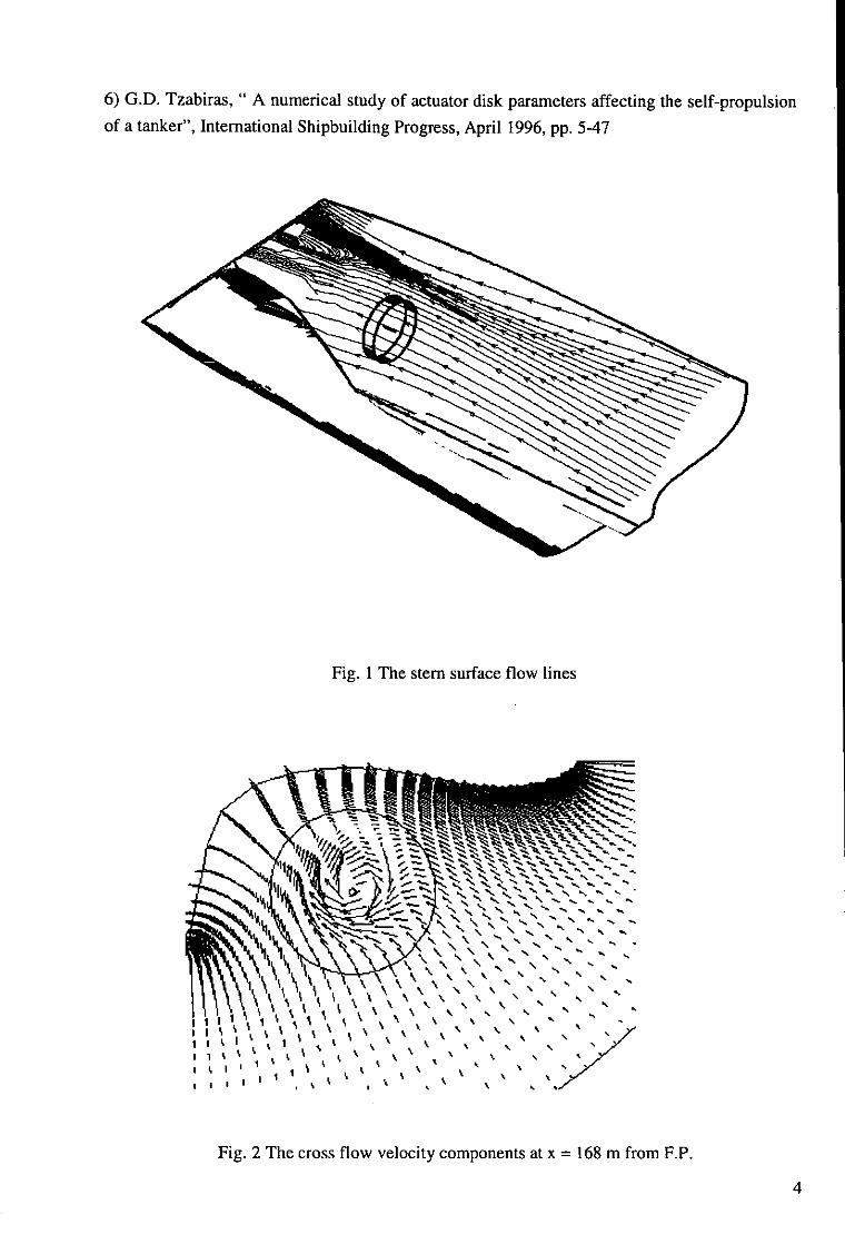
6) G.D. Tzabiras, " A numerical study of actuator disk parameters affecting the self-propulsionof a tanker", International Shipbuilding Progress, April 1996, pp. 5-47

Fig. 1 The stem surface flow lines

I ¶1 \ '. '

I I>

Fig. 2 The cross flow velocity components at x = 168 m from F.P.

4

OBLIQUE VISCOUS FLOW AROUND A TWIN SKEG TANKER MODEL

Mathias Vogt, Hamburg Ship Model Basin, email: vogt@hsva.de

INTRODUCTIONA twin-skeg ice-breaking tanker is to be dynamically positioned i.e. to be held in a fixed position under theinfluence of forces from the fluid flow, for instance current, wind and waves, acting on the hull. To stay in afixed position the ship has to generate corresponding forces with its own propulsion systems.

With an inlet velocity U=0.253 m/s, the flow around the tanker is computed for different drift angles, A3 between0 and 500 with an in-house RANSE solver Neptun. Neither the free surface nor the propeller were taken intoaccount in the computations. Due to the very low inlet velocity, the wave induced drag was considered negligibleand the propellers were omitted to avoid even more difficulties by the grid generation. The ships maindimensions are: length L=228 m, draft D=13 mn and breadth B=32 mn. Computations were made for the draftD=0.3714 mn of the model corresponding to D=13 mnat full scale and for the deep water case. In the model testsit was shown that there were no tank floor influences for a water depth of 25 mn (0.7 14 mn at model scale). TheReynolds number was Rn= 1.65 106.

METHODThe viscous oblique flow is computed solving the Raynolds averaged Navier-Stokes equations and the continuityequation. Reynolds stresses are modelled with a k-w turbulence model and here wall functions were used.

The conservation equations are discretised on a body fitted non-matching block structured grid using a finitevolume method. All unknowns are defined at the cell centres. The diffusion terms are approximated with centraldifferences and the convected velocities in the momentum fluxes with the linear upwind differencing scheme.Mass fluxes are interpolated according to Rhie and Chow and the SIMPLE algorithm is used to solve theresulting system of non-linear equations. For a more detailed description of the method see [31.

On the hull the no slip condition is enforced. Slip condition was used on the outer horizontal boundary, thesymmetry plane and for 03=00 on the outer lateral boundaries. At the inlet planes, undisturbed flow was assumedi.e. velocity is prescribed and the turbulent kinetic energy, k=10' 5 and its specific dissipation rate, ow-10. At theoutlet planes, the homogeneous Neumann condition was used for the velocities and the turbulent parameterswhile the Dirichlet condition was used for the pressure.

GRIDDifferent from a symmetrical computation, a grid on both sides of the ship is needed in the non-symmetricalcase, which implies larger computational domain and more grid nodes. Since the free surface and effects thereofe.g. sinkage and trim (Froude number based on the depth Fn«<0.5) play a minor role here, the double body caseis considered. The inlet was placed at one ship length in front of the FP, the outlet at one ship length behind theAP and the side boundaries as well as the bottom boundary were placed one ship length away from the symmetryplanes. With 34 patches on one side of the hull, of which most of them in the stem region, half of the grid wasbuild with about 80 blocks. Many of these were matching and could have been merged giving a grid with fewerblocks. The grid consisted of a total of 350 000 cells. Figure 1 shows a part of the hull surface grid at the stemand at the stern including a grid surface in a block outside the hull. It can be seen how the fore body, rudders,stern tunnel and the stern tubes are discretised to avoid grid singularities.

COMtENTS ON THE COMPUTATIONSTo numerically solve these kinds of problems is difficult and it becomes more and more difficult to achieveconvergent solutions with higher drift angles since the flow is fully non-symmetrical and partly highly turbulent.Another reason is that the strong main stream becomes less significant with higher drift angles. Further, the fluidflow is more complex than for the case of a symmetrical flow, with vortex generation, separation andreattachment at the stern but also at the stem. So, it is usually not possible to reach a satisfactory convergence forlarger drift angles (>200). In figure 7 the fully unsymmetrical pressure distribution for P3=500 is shown. Lately,more papers have addressed related topics. In [ 1,2,4,5] the well known Series 60 ship was chosen as a test case.Measurements are available for P-<200 and results for larger angles might therefore not have been reported.

In the computed case an additional difficulty was the very weak flow around the tanker, which yields a very lowmodel Reynolds number. Consequently, laminar effects that could be strongly different from side to side at non-symmetrical flows could appear. The commonly used turbulence models cannot or can only very roughly predicttransition from a laminar flow to a turbulent flow. For instance, the k-w model predicts it too early. Therefore, it

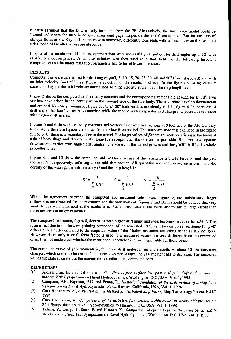
is often assumed that the flow is fully turbulent from the FP. Alternatively, the turbulence model could be'turned on' where the turbulence generating sand paper stripes on the model are applied. But for the case ofoblique flows at low Reynolds numbers with unknown, differently long parts with laminar flow on the two shipsides, none of the alternatives are attractive.

In spite of the mentioned difficulties, computations were successfully carried out for drift angles up to 500 withsatisfactory convergences. A laminar solution was then used as a start field for the following turbulentcomputation and the under relaxation parameters had to be set lower than usual.

RESULTSComputations were carried out for drift angles 03=0, 5 ,10, 15, 20, 25, 30, 40 and 500 (from starboard) and withan inlet velocity U=0.253 m/s. Below, a selection of the results is shown. In the figures showing velocitycontours, they are the axial velocity normalised with the velocity at the inlet. The ship length is L.

Figure 2 shows the computed axial velocity contours and the corresponding vector field at 0.2L for #3=100. Twovortices have arisen in the lower part on the leeward side of the fore body. These vortices develop downstreamand are at 0.3L more pronounced, figure 3. For P3=300 both vortices are clearly visible, figure 4. Independent ofdrift angle, the 'keel' vortex stays attached while the second vortex separates and changes its position even morewith higher drift angles.

Figures 5 and 6 show the velocity contours and vectors fields of cross sections at 0.95L and at the AP. Contraryto the stem, the stern figures are shown from a view from behind. The starboard rudder is excluded in the figure5. For OW=00 there is a secondary flow in the tunnel. For larger values of P3 there are vortices arising at the leewardside of both skegs and the one in the tunnel is stronger than the one on the port side. Both vortices separatedownstream, earlier with higher drift angles. The vortex in the tunnel growes and for 63=300 it fills the wholepropeller tunnel.

Figure 8, 9 and 10 show the computed and measured values of the resistance X', side force Y' and the yawmoment N', respectively, referring to the mid ship section. All quantities are made non-dimensional with thedensity of the water p, the inlet velocity U and the ship length L:

X x=-- Y',= N'= NP L2U2 P L2U 2 P LU 2

2 2 2

While the agreement between the computed and measured side forces, figure 9, are satisfactory, largerdifferences are observed for the resistance and the yaw moment, figures 8 and 10. It should be noticed that verysmall forces were measured at the model tests. Such measurements are more susceptible to large errors thanmeasurements at larger velocities.

The computed resistance, figure 8, decreases with higher drift angle and even becomes negative for P3Ž35'. Thisis an effect due to the forward pointing component of the generated lift force. The computed resistance for /=0 °

differs about 30% compared to the empirical value of the friction resistance according to the I'TTC-line 1957.However, there only a small form factor is used. The measured values are very different from the computedones. It is not made clear whether the mentioned inaccuracy is alone responsible for those or not.

The computed curve of yaw moments is, for lower drift angles, linear and smooth. At about 300 the curvaturechanges, which seems to be reasonable because, sooner or later, the yaw moment has to decrease. The measuredvalues oscillate strongly but the magnitude is similar to the computed ones.

REFERENSES[1] Alessandrini, B. and Delhommeau, G., Viscous free surface low past a ship in drift and in rotating

motion, 22th Symposium on Naval Hydrodynamics, Washington, D.C.,USA, Vol. 1, 1998[2] Campana, E.F., Esposito, P.G. and Penna, R., Numerical simulation of the drift motion of a ship, 20th

Symposium on Naval Hydrodynamics, Santa Barbera, California, USA, Vol. 1, 1994[3] Cura Hochbaum, A., A Finite-Volume Method for Turbulent Ship Flows, Ship Technology Research 41/3

1994[4] Cura Hochbaum, A., Computation of the turbulent flow around a ship model in steady oblique motion,

22th Symposium on Naval Hydrodynamics, Washington, D.C. USA, Vol. 1, 1998[5] Tahara, Y., Longo, J., Stern, F. and Himeno, Y., Comparison of cfd and efd for the series 60 cb=0.6 in

steady yaw motion, 22th Symposium on Naval Hydrodynamics, Washington, D.C.,USA Vol. 1, 1998

Fig.1 Views of the numerical grid.

,- -, -:. - - - - -- - _- - • - _ _

... .- - -: i i- - - --- -- : : : :- _ -. .. .--

Fig.2 Computed velocity field for /3 100 at 0.2L.

----- -- - ------

Fig.3 Computed velocity field for / 100 at 0.3L.

Fig.4 Computed velocity field for /3 = 30' at 0.3L.

-t -c - -------

Fig.5 Computed velocity field for 13300 at 0.95L.

'A.

------------------

L -- J

r --- -- -- ----

r I i - 7 - -i- -i

Fig.? Computed pressure distribution for /3=500. Fig.8 Measured and computed resistance vs. /

30~~ - - -- - - - - -------- ---

2 6 - E O I S -2-- -OW : I II I I I

20~4 L4J5.. L L. 0L 0 45 W

Ii. Mesue an copue s id foc vs Ii Mesue an copue ya moets

Viscous Flow Prediction around a VLCC using Adaptive Grid Techtniques

Peter Bull, Stephen Watson, Defence Research and Evaluation Agency, Haslar

This work is part of an ongoing programme to predict the full scale flow around a fully appended, powered ship.The primary objective of the work is to realise the potential of Reynolds Stress Models (RSM) in conjunctionwith solution adaptive grid techniques for a ship hull. The nominal wake as typified by a VLCC is a stage on thisroute. Flow predictions are made using both fixed and adaptive grids to the VLCC and several simplergeometries. The second aspect of the work addresses the consequences of the particular form of the dissipationrate equation. The object of this analysis is to form a basis to separate local effects from history effects.Observations are made on the basis of consistency when one turbulence model is allowed to develop on fixedvelocity fields, which have been predicted by other turbulence models. Where possible, analytic estimates ofsource differences are developed.

Introduction

The quality of predictions of viscous flows around marine structures has always been dependent on bothturbulence model and grid. With decreasing computing cost, very large grids of high quality can be built, onwhich predictions exhibit grid independence under widening range of conditions. In consequence, the differencesdue to choice of turbulence model are becoming clear to see. For ship hydrodynamics, the questions are whatorder of modelling is appropriate, when and why.

Second moment Reynolds stress closures are recognised as a general and powerful class of turbulence models,but not as the most efficient. RSM is becoming common place because the requisite technical knowledge iswidespread, on average they are better than other models, and their computing costs are reducing. However, ahallmark of the last thirty years is that increased generality has produced better predictions only on average,rather than consistently. There is a danger that this will only be compounded when grid adaptation is added tothe solution process.

To provide a validation path, several geometries were chosen to prototype the viscous flow and grid adaptationon the basis that structured grids of high quality could be generated:

1. boundary layer with an adverse pressure gradient / a finite flat plate2. flow through an axi-symmetric diffuser3. thick axi-symmetric boundary layer on a cylinder4. axi-symmetric flow past a body of revolution (supported by by struts)5. flow past a modified Wigley hull

The boundary layer was chosen the weight of analysis that can be brought to bear on it. The axi-symmetric flowswere chosen because they exhibit the loss of the logarithmic overlap within the hull shear layer. The flowthrough the diffuser while simple geometrically presents significant difficulties for most of the currentgeneration of turbulence models. Finally, the modification of the Wigley hull introduces weak secondary flowsover an intermediate ship-like geometry, and was suggested by model tests reported by IHI at the first Osakacolloquium in 1987. Potentially, these secondary flows can be introduced in a gradual manner through varyingthe parameter controlling the fullness of the form.

Predictions are to be made on fine block-structured grids in order to base-line the adaptive predictions. The flowadaptation is initially being made of the basis of geometric curvature of boundaries and flow gradients. Theunstructured grid approach is hybrid with prisms, possibly degenerate, being grown from viscous boundaries andabove which, the interior is filled with tetrahedra (see Figure 1).

Flow Predictions around VLCC

Work to date has centred on the VLCC geometry itself to scope the potential effects of geometric quality on theadaptive process and to identify associated problems not inherent in the simpler geometries within the program.

The RSM chosen for the predictions the VLCC is the Launder Reece Rodi model. Given the problems associatedwith constructing wall reflection, the model for the pressure-strain correlation due to Speziale, Sarkar & Gatskihas been used. The RSM predictions are initialised by RiNG k-g predictions on the coarsest grid. The initial

Reynolds stresses are estimated from the standard isotropic k-s model of the stresses, but clipped so that theysatisfy the Schwarz inequality. Standard wall functions have beenused; it is intended vary details of theirformulations in future calculations.

Grid adaptation has been limited to three grid refinements. No adaptation is performed nornal to the hull in theprism layers. Grid coarsening is limited to the coarsest grid level. Although moderately well-convergedpredictions have made (see Figure 2), problems arising from geometry are posing problems to further adaptationof the solution. This primarily because the underlying geometric surfaces are used within the adaptation process.

The definition of the geometry was the IGES file posted on the Gothenburg 2000 web site. The geometry definedwithin this file was somewhat imperfect, particularly near the keel at the junction of the bow and the main hull.A certain amount of redefinition of geometry was undertaken via bi-cubic patches. The modified definition hasnot yet been checked against the original file and point definitions (also posted). However, we believe our re-defined geometry is close to original over the majority of the hull. Even so, the curvature of the hull on themodified region is still a matter for concern as there is excessive adaptation to this region, not warranted by theflow itself (see Figure 3).

Analysis of turbulent dissipation rate

For RSM to produce significant benefits consistently, the key controlling performance need to be clearlyhighlighted. For example, the treatment of wall reflection terms is important for wall bounded flows. YetWilcox' has suggested that the major benefit of wall reflection treatments makes good the deficiencies of thedissipation rate equation, rather than as a fundamental aspect of the RSM model.

The weakness for turbulence models based on single-point closures of whatever order is the equation for thedissipation terms in the Reynolds stress equations which is complex and subject to many assumptions andapproximations. Nevertheless, the Reynolds stresses are dependent on both velocity and length scales. For RSM,this dependence is implicit as it is for one-equation models such as Baldwin-Barth and Spalant-Allmaras; for twoequation models, the relationship is explicit.

For certain cases such as the development of a boundary layer on a flat surface, the implications of the form ofthe dissipation equation can be assessed. For example, on the basis of perturbation analysis, Takemitsu2 suggeststhat the k-s model requires modification to exhibit a wall function solution, while Wilcox, 3 suggests that his k-tOmodel can be integrated through the laminar sub-layer and that the to equation does exhibit a wall functionsolution for channel flow. A similar type of analysis by Wilcox and HenkeS3 indicates that for boundary layerswith adverse pressure gradients, SMCs, k-a) and at least one algebraic mode! outperform k-s model in accuracyof predictions. While Wilcox's to equation appears better behaved than an E equation, the to equation is anapproximation and by no means certain that it will perform well in all cases and that the to equation an optimumprescription. This suggests the question - what form would a differential length scale equation have to take toreproduce, or even to outperform an algebraic model consistently? Regarded only as systems of model equations,such modifications to differential turbulence models are easy to contemplate. For example, althoughhomogeneous turbulence decays in the absence of velocity gradients, the asymptotic behaviour of higher ordermodels can easily be altered to reproduce the constant levels predicted by simpler models via sources forprescribed values of k,; TisEand to.

The starting points for most turbulence models are averaged moments of the Navier-Stokes equations. Thestandard k equation is derived from the equation for the trace of the Reynolds stresses and by approximating thetwo remaining unclosed correlations. The original equation and the derived k equations are relativelyuncontroversial, and therefore are used as a basis for comparison, together with a set of algebraic stress models.Using these equations, differential length scale equations are developed for the Baldwin-Barth, Spalart-Allmarasand Baldwin-Lomax models via MAPLE 6. In the first instance, the distance to the nearest wall is left as anunclosed function. The differences in source terms between the derived equations and the E equation are derivedand evaluated for the simple geometric cases and numerically for the VLCC.

1. Wilcox. 1998. Turbulence Modelling for CFD. DCW Industries.2. Takemnitsu. 1990. An Analytic Study of the Standard k-E Model. J. Fluids Eng. 112. pp 192-198.3. 1-enkes. 1998. Scaling of Equilibrium Boundary Layers Under Adverse Pressure Gradients Using

Turbulence Models. AIAA 36.3. pp.320-326.

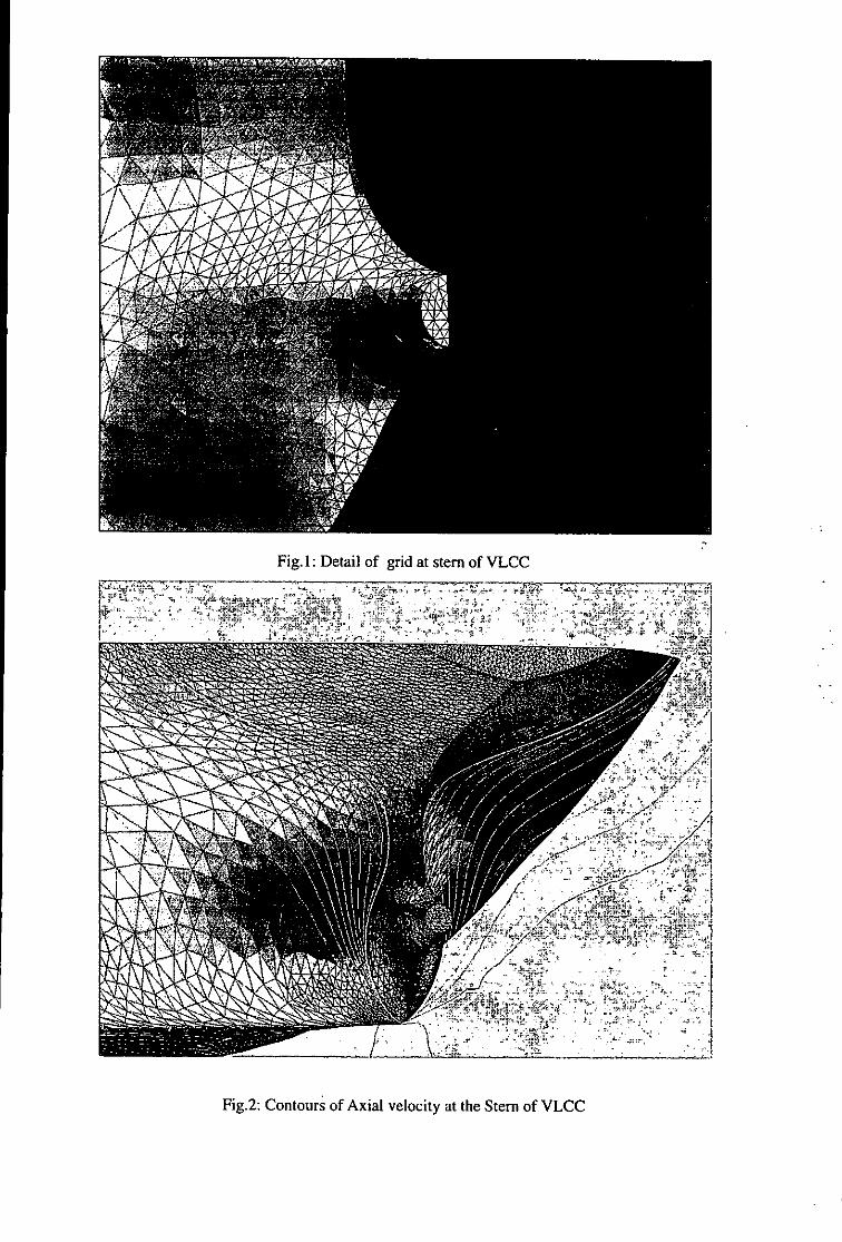
Fig. 1: Detail of grid at stem of VLCC

- ~5-

. ~ ~ aPt

Fig.2: Contours of Axial velocity at the Stem of VLCC

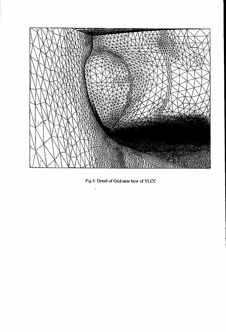
Fig.3: Detail of Grid near bow of VLCC

A composite procedure for ship viscous flow with free surface

JAAP W[NDT, HOYTE C. RAVENMaritime Research Institute Netherlands (MARIN), P.O. Box 28, 6700 AA Wageningen, Netherlands

1 Introduction

One of the most active fields of ship hydrodynamics research today is the development of methods for comput-ing the steady viscous flow with free surface around a ship hull. Compared to the classical separate considerationof wave making and viscous flow, such methods aim at making a step forward by incorporating free-surfaceeffects on the viscous flow, and viscous effects on the wave pattern. Methods proposed generally solve theRANS equations subject to dynamic and kinematic free-surface boundary conditions (FSBC's).

While appreciable progress has been made in recent years, the problem is not really solved yet. Mostlya good prediction of the wave profile along the hull is obtained, but the wave pattern away from the hull usuallyis rather poor due to substantial numerical damping, unless dense grids with several millions of cells are used.Moreover, virtually all methods consider a time-dependent problem and integrate in time until a steady resultis obtained; but the approach to steady state may be quite slow due to transient waves, reflections at openboundaries, and small permissible time steps. The resulting large calculation times and reduced robustnesscomplicate the effective use in practice and make it hard to achieve grid-independent solutions, in particular forlower Froude numbers. Consequently, these methods are only rarely used routinely in ship design.

Most RANS computations in practical ship design therefore still use a double-body approximation.However, a step forward is possible without any significant computation time penalty. As many validationshave demonstrated, inviscid methods can predict most of the wave pattern very efficiently and accurately. Anobvious procedure therefore is to first run a panel code to determine the wave pattern, and next to compute theviscous flow, imposing free-slip boundary conditions at the wave surface. In this non-interactive formulation,most free-surface effects on the viscous flow are taken into account, but not the viscous effects on the wavepattern, which are known to be localised near the stem.

Surprisingly, this possibility seems to have been largely disregarded so far, except for the similar workat NTUA [6] in which viscous flow was computed under a measured wave surface.

2 The composite procedure

Wave pattern calculation The first step is the calculation of the wave pattern, using a nonlinear free-surfacepotential flow method. We use the code RAPID[l]1, an iterative 'raised-panel' method using a source distributionon the hull surface and on a surface at a specified distance above the wave surface. On the hull, zero normalvelocity is imposed; in collocation points on the wave surface, the kinematic condition (flow tangential to thewave surface) and the dynamic condition (pressure atmospheric at the wave surface) are imposed. Iterationcontinues until both conditions are satisfied, and until there is no further change of the wave elevation and thetrim and sinkage of the ship. The method is known to predict the wave pattern accurately, with as principalexception the overestimation of the stem wave system due to the neglect of viscous effects.

free surface

hull & a minet vlane

Zmine lane0"0M0

Figure 1: Grid used in viscous flow calculation under precomputed wave surface. Only every second line in each direction shown.

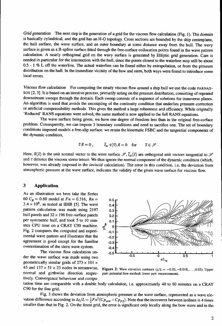
Grid generation The next step is the generation of a grid for the viscous flow calculation (Fig. 1). The domainis basically cylindrical, and the grid has an H-0 topology. Cross sections are bounded by the ship centreplane,the hull surface, the wave surface, and an outer boundary at some distance away from the hull. The wavysurface is given as a B-spline surface fitted through the free-surface collocation points found in the wave patterncalculation. A nearly orthogonal grid on the wavy surface is generated by Elliptic grid generation. Care isneeded in particular for the intersection with the hull, since the points closest to the waterline may still be about0.5 - I % L off the waterline. The actual waterline can be found either by extrapolation, or from the pressuredistribution on the hull. In the immediate vicinity of the bow and stem, both ways were found to introduce somelocal errors.

Viscous flow calculation For computing the steady viscous flow around a ship hull we use the code PARNAS-sos [2, 3]. It is based on an iterative process, primarily acting on the pressure distribution, consisting of repeateddownstream sweeps through the domain. Each sweep consists of a sequence of solutions for transverse planes.An algorithm is used that avoids the uncoupling of the continuity condition that underlies pressure correctionor artificial compressibility methods. This gives the method a large robustness and efficiency. While originally'Reduced' RANS equations were solved, the same method is now applied to the full RANS equations.

The wave surface being given, we have one degree of freedom less than in the original free-surfaceproblem. Consequently, we can impose 3 boundary conditions and need to sacrifice one. The set of boundaryconditions imposed models a free-slip surface: we retain the kinematic FSBC and the tangential components ofthe dynamic condition,

.h = 0, ?a.tr(V)A = 0 for Y E .

Here, fl(i) is the unit normal vector to the. wave surface Y', ta (1) are orthogonal unit vectors tangential to Yand z denotes the viscous stress tensor. We thus ignore the normal component of the dynamic condition (which,however, was already imposed in the inviscid calculation). The error in this condition, i.e. the deviation fromatmospheric pressure at the wave surface, indicates the validity of the given wave surface for viscous flow.

3 Application

As an illustration we here take the Series60 CB = 0.60 model at Fn = 0.316, Rn = 0.53.4 x 106, as tested at IMH [5]. The wave 0.pattern calculation was made using 2197 0.3hull panels and 32 x 196 free-surface panels 0.2per symmetric half, and took 5 to 10 min- 0.1utes CPU time on a CRAY C90 machine. 0 0Fig. 2 compares the computed and experi- -0.1mental wave pattern and illustrates that the -0.2agreement is good except for the familiar -0.3overestimation of the stem wave system. -0.4

The viscous flow calculation un- -0.5 I I I , I , ider the wave surface was made using two 0.5 0 0.5

geometrically similar grids of 273 x 101 x45 and 137 x 51 x 23 nodes in streamwise, Figure 2: Wave elevation contours (z/L = -0.02,-0.018,... 0.02). Uppernormal and girthwise direction respec- part: potential flow method; lower part: measurements.tively. Convergence behaviour and compu-tation time are comparable with a double body calculation, i.e. approximately 40 to 60 minutes on a CRAYC90 for the fine grid.

Fig. 3 shows the deviation from atmospheric pressure at the wave surface, represented as a wave ele-vation difference according to Az/L = 1Fn2 (Cpa,,, - CpFs). Note that the increment between isolines is 4 timessmaller than that in Fig. 2. On the finest grid, the error is significant only locally along the bow wave and in the

2

0.2

0.10 ............

-0.1

-0.1 -' - - ' 9 A

-0.6 -0.4 -0.2 0 0.2 0.4 0.6 0.8 1X/L

Figure 3: Pressure deviation at wave surface, related to wave elevation.(Az/L= -0.02,-0.0195,... 0.02\{0.0}). Upper part: finegrid; lower part: coarse grid.

_O-0.06 - _06 I0I

•0•' t% Om ,M - ON, Off i)00 .•06 4-.M A02 • OM 0124 ON • O"M WM 10 4}0 _ loM A .02 ON¢ 0{'

Intgfli 0. ... . ......gm.. h n In

k\ k

"0.06 006 ll t/l I , ll IlII

' P ~ K K t- o~ o~~- 0 00 0 0 \ \ \0.0 * • Uti 'I , -0.04 - ,,4.,:-

_aM,-00 0.00 0.02 0.0 4002 0,06 0.0 0,0 W00 . .2 00y/L y/L, Y/L

Figure 4: Axial and transverse velocity field at x/L = 0.2 (upper part) and x/L = 1.0 (lower part). The figures to the left show themeasurements[5], the figures at the middle and at the right show the predicted wake field using the double body approach (left) and(one step) composite procedure (right).

stem area, and is negligible everywhere else (less than 0.0005 L, or 2.7 % of the maximum wave elevation).Comparison of the coarse and fine grid solutions, and of intermediate solutions obtained by the successive gridrefinement stages of the solution procedure 1, shows excellent convergence of the pressure distribution on thewave surface by grid refinement. At most places it converges to almost zero, indicating that the pressure devia-tions are only due to discretisation errors in the finite-difference solution. Some disturbances do not disappearupon grid refinement, and these are caused by viscous effects on the wave pattern, or to discretisation errors inthe inviscid solution.

If the calculated pressure differences would be simply used to correct the wave elevation, they wouldindeed reduce the stem wave height; but iteration is then needed to account for the wave pattern changesdownstream. But such changes have no significant effect upstream, so it may well be concluded that a validRANS/FS solution has been obtained everywhere except the stem wave system itself and in the wake.

Fig. 4 shows the computed axial and transverse velocities for two x = constant planes using thedouble-body approach and the (one step) composite procedure. As expected, the quality of the predicted axialand transverse velocities close to the waterplane improves definitely by the composite approach. However the

1. using 35 x 51 and 69 x 51 nodes (coarse grid) and 69 x 101 and 137 x 101 nodes (fine grid) on the wave surface.

3

longitudinal vortex in the wake seems to be overshadowed by the vertical velocity. The latter is most likelysomewhat too large due to the overestimation of the stem wave system, but further investigation is essential.First of all, for accurate wake field prediction we need to (and intend to) apply a more appropriate turbulencemodel like the Menter model or k - wo model. Secondly, the stepsize in streamwise direction is too large toobtain a grid independent solution (we used an equidistant node distribution, focusing on the pressure on thewater surface). Both changes usually improve the prediction of longitudinal vortices.

4 Discussion and conclusions

In the calculations made so far, the major free-surface effect on the viscous flow was found to be non-interactive,and can be captured in a single step of the composite approach. The pressure difference across the wave surfacepartly results from the different numerical methods used in the inviscid and viscous calculations, and then wasfound to vanish upon grid refinement; partly it indicates where viscous effects on the wave pattern are present.The latter indication is very well correlated with the location of observed differences of the wave elevation withexperimental data, and is a very limited area aft of the stern.

The method proposed disregards this viscous effect on the wave pattern, and the additional 'dis-placement effect' of the boundary layer and wake. In a recent study also the latter has been found to be onlysignificant for the stem and near wake area. A full, interactive RANS/FS solution would be needed there (butonly there) to include these effects.

The application considered is a slender hull form, and for fuller hull forms a stronger (and sometimesqualitative) change of the wave elevation due to viscous effects takes place. However, even in those cases thosechanges are confined to the stem area. On the other hand, the case studied here exaggerates the wave/viscousinteraction, due to the unusually low Reynolds number and the rather high Froude number, and the presence ofa cusped stern.

Therefore, the composite procedure proposed here for most of the domain can provide a solutionequivalent to a full RANS/FS solution on a dense grid, with an effort just marginally larger than that for adouble-body RANS solution. This easy and most efficient procedure will soon replace the double-body ap-proach for most of our practical computations. The task of RANS/FS can then be limited to the stem areawhere it is really needed. Work on a new RANS/FS method, solving the steady problem by iteration, is under-way [4], and will hopefully supplement the composite procedure.

References

[1] Raven, H.C., "Inviscid calculations of ship wave making - capabilities, limitations and prospects", 22ndSymp. Naval Hydrodynamics, Washington DC, 1998.

[2] Hoekstra, M., "Numerical simulation of ship stem flows with a space-marching Navier Stokes method",Thesis, Technical University of Delft, October, 1999.

[3] Van der Ploeg, A., Hoekstra, M., and Eca, L., "Combining accuracy and efficiency with robustness in shipstem flow computation", 23rd Symp. Naval Hydrodyn., Val de Rueil, France, 2000.

[4] Raven, H.C., and Van Brummelen, H., "A new approach to computing steady free-surface viscous flowproblems", 1st MARNET-CFD workshop, Barcelona. To be downloaded from http: / /www. marin.nl/publications/pgresistance .html

[5] Toda, Y., Stern, F, and Longo, J., "Mean-flow measurements in the boundary layer and wake field of aSeries 60 Cb = .6 ship model for Froude numbers .16 and .316 IIHR Report No. 352, Iowa Institute ofHydraulic Research, August, 1991.

[6] Garofallidis, D.A., "Experimental and numerical investigation of the flow around a ship model at variousFroude numbers," Doctor's Thesis, National Techn. Univ. Athens, 1996.

4

Nonlinear Time Domain Analysis of Ship Motionsin Regular Head Waves

Hironori YASUKAWA, Nagasaki Experimental Tank, Mitsubishi Heavy Industries*

Introduction

In this paper, we propose a nonlinear time domain analysis method of ship motions in waves.This method can be regarded as an extension of the method for free-surface flow of a high speedvessel proposed in NuTTS'99[1]. In the previous paper, no ship's attitude change was assumed.We put a scheme of ship motion computation to the original method for the free-surface flows bya panel method. As a result, it becomes possible to compute wave-making resistance includingeffect of attitude change, and ship motions in waves including nonlinearity of free-surface and hullboundary conditions. We present the computed results of ship motions and wave deformationsin regular head waves for a modified Wigley hull.

Basic Equations

Let us consider a ship advancing in a towing tank. It is assumed that a ship moves with speedU(t) which varies as the function of time t. The coordinate system fixed in the space is employed.The x-axis is defined as direction from ship stern to the bow, y-axis to port and z-axis verticallyupward. The x - y plane is the still water surface. Deep water is assumed.

3 ship's motion displacements with respect to surge, sway and heave in the fixed coordinatesystem are defined as Gi, ý2, b respectively, and the vector C. Euler angles with respect to roll,pitch and yaw are represented as ýp, 0, 4 respectively, and the vector n. Incident waves aregenerated by the flap-typed wave maker attached tank wall.

The perturbation velocity potential due to ship moving in the tank is defined as q(x, y, z, t).Then, q5 has to fulfill the following boundary conditions:

a't -g -g( a2V0) 2 on z = 0 (1)

aq5 a20 a a( ao a(-- + -( -z - - y onz=O (2)at 19 aZ2 Ox ax ay ay

8 -__(v+wxr).n onSH (3)an-" v0 on Sw (4)

where V = Co, •, •)" e denotes wave height, g the gravity acceleration. SH and Sw meanhull and tank wall surfaces respectively.

Eqs.(1) and (2) are free-surface conditions employed in this paper. For simplicity, we employthe 2nd order conditions with respect to 4 and ( obtained by Taylor expansion at z = 0. Eq.(3)is hull surface condition, and has to be satisfied on actual wetted surface SH. Here v denotesship velocity vector defined in the coordinate system fixed to ship, and w the angular velocityvector. v includes the component of ship speed U(t). Relations between v and C, and betweenw and 0 are as follows:

v - [E(0)]t, w = [H( 0 ) 0 ( (5)

where

*3-48 Bunkyo-Machi, Nagasaki 852-8131, JAPAN, email: yasukawa@ngsrdc.mhi.co.jp

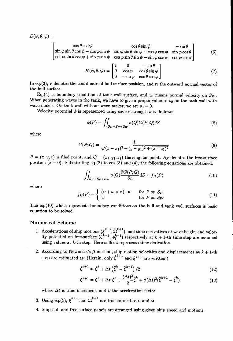
E(, O, i) =

cos O cos V 0 sinV - sin Isin vo sin 0 cos V - cos W sin 7 sin W sin 0 sin V + cos ýo cos, sin ecos01 (6)cos Wsin0cos + sinqWsin47 cos'Wsin0sinV- sinoVscosP ocos 0

1l 0 - sin 0H(W, 0,,0) = 0 cos W0 cos 0: sin Wo (7)

0- sinW cos0cosWoIn eq.(3), r denotes the coordinate of hull surface position, and n the outward normal vector ofthe hull surface.

Eq.(4) is boundary condition of tank wall surface, and vo means normal velocity on Sw.When generating waves in the tank, we have to give a proper value to v0 on the tank wall withwave maker. On tank wall without wave maker, we set vo = 0.

Velocity potential q5 is represented using source strength a as follows:

O(P) ILU+SF+SW a(Q)G(P; Q)dS (8)

where

G(P;Q) -- X( x - X1 )2 + (y- Yl) + (z -z) 2 (9)

P = (x, y, z) is filed point, and Q = (xi, yi, zi) the singular point. SF denotes the free-surfaceposition (z = 0). Substituting eq.(8) to eqs.(3) and (4), the following equations are obtained:

ILHSNF+sw a(Q) ; Q) dS = fH(P) (10)

where= I' (v+wxr)-n forPonSH

vH for P on Sw

The eq.(10) which represents boundary conditions on the hull and tank wall surfaces is basicequation to be solved.

Numerical Scheme

1. Accelerations of ship motions ( k+l, fik+l), and time derivatives of wave height and veloc-ity potential on free-surface (Ct+l, ok+1) respectively at k + 1-th time step are assumedusing values at k-th step. Here suffix t represents time derivation.

2. According to Newmark's /3 method, ship motion velocities and displacements at k + 1-thstep are estimated as: (Herein, only k+1 and Ck+l are written.)

k+= + tk Wk+ t kg l)/ 2 (12)

Ck+l - Ck +•At tk 2 ( Ck ±-l(At)2(Ck+l -C 4k) (13)

where At is time increment, and /3 the acceleration factor.

3. Using eq.(5), Ck+l and fk+l are transformed to v and Lo.

4. Ship hull and free-surface panels are arranged using given ship speed and motions.

5. According to Newmark's fi method, wave height and velocity potential on free-surface atk + 1-th step are estimated as:

(k+1 = + At + ck+1) /2, 0k+1 = + At + ok+1) /2 (14)

6. Influence functions are calculated for free-surface, ship hull and tank wall surfaces to makea matrix for determining source strength. Basic equations are discretized using constantpanels.

7. Solving eqs.(8) and (10), source strengths on free-surface, hull and tank wall surfaces areobtained.

8. Using eqs.(1) and (2), 0Ak+ and (-k+1 are calculated. Then, velocity components on free-surface are calculated analytically using the source strengths. The derivatives of ( withrespect to x and y are obtained numerically using finite differential technique.

9. Hydrodynamic forces acting on hull are calculated by Bernoulli's equation. Obtaining thehydrodynamic forces, i) and 6i are calculated from the motion equations of the ship.

10. Using eq.(5), b and cb are transformed to C and 1?.

11. C, iý, (• and St obtained in step 8 and 10 are compared with those assumed in step 1.When the difference between both is sufficiently small, ý, 6, (t and Ot are regarded asreaching to the convergence. Otherwise, return to step 2 and calculations are continuedusing f, f(, Ct and Ot obtained in step 8 and 10 until obtaining converged solution throughthis iteration.

12. One time step is increased and return to step 1.

Computed Results

Analysis of ship motions in regular head waves for a modified Wigley Hull is carried out. Thehull is a mathematical form expressed as follows:

Y (1 - x'")(1 - z'2)(1 + 0.2x' 2 ) + z' 2 (1 - z'8 )(1 - x'12 )4 (15)where x' = x/(L/2), y' = y/(B/2), z' = z/d

with LIB = 10.0 and Bid =1.6. The calculated results are compared with experimental dataconducted in Delft University. To obtain the experimental data, we read the data from figuresin the paper presented by Sclavounos et al.[2J who used the data for comparison with theircalculated results.

In the present computations, a numerical absorbing beach is put to only face-side wall againstwave maker. As the absorbing technique, we apply the method proposed by Cointe et al.[31where proper damping is added to free-surface conditions. On side walls, we don't impose anynumerical beach technique and allow of wave reflections similar to actual towing tank.

Fig.1 shows comparison of heave and pitch. Froude number based on ship length F. is 0.3.4000 panels for free-surface, 2400 panels for tank wall, and 800 panels for ship hull are used.Computed wave amplitude of incident wave is about 0.0025L. The calculated amplitude andphase angle for heave and pitch are agreed well with experiments.

Fig.2 shows 2 snap shots of the computed wave patterns generated by a modified Wigley hulladvancing in regular head waves with A/L=1.0. In the figure, wave contours are shown of 0 and90deg for phase angle against incident wave from the top. The steady Kelvin waves, incidentwaves, scattering waves and reflected waves at tank side walls are realistically demonstrated.

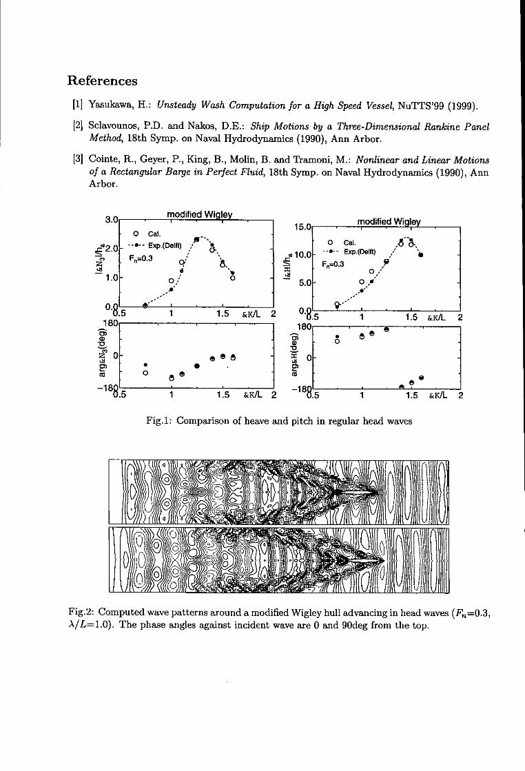
References

[11 Yasukawa, H.: Unsteady Wash Computation for a High Speed Vessel, NuTTS'99 (1999).

[2] Sclavounos, P.D. and Nakos, D.E.: Ship Motions by a Three-Dimensional Rankine PanelMethod, 18th Symp. on Naval Hydrodynamics (1990), Ann Arbor.

[3] Cointe, R., Geyer, P., King, B., Molin, B. and Tramoni, M.: Nonlinear and Linear Motionsof a Rectangular Barge in Perfect Fluid, 18th Symp. on Naval Hydrodynamics (1990), AnnArbor.

3.0 modified Wigley 15.0,modified Wigley0 Cal.

42.0 -- 0-- Exp.(Delft) 0 Cl.(

F-o=0 • 10.0 - - p.(D m)Fn. F---0.3

10 0 5.0 0,,d

A'A

.5 1 1.5 &K/L 2 o.85 1 15 &K/L 2180 180

0 1 '0

I 1888. 1 1.5 &KIL 2 '8.5 1 1.5 &K/L 2

Fig.1: Comparison of heave and pitch in regular head waves

0)0Fig.2: Computed wave patterns around a modified Wigley hull advancing in head waves (F,=0.3,A/L=1.0). The phase angles against incident wave are 0 and 90deg from the top.

4th Numerical Towing Tank Symposium (NuTTS'01)

Hamburg, Germany, 23-25 September 2001

Topics:

" Nonlinear flows around marine structures (LES, RANSE, Euler with or w/o free surface)" Free-surface flows around marine structures (3-d ship seakeeping, free-surface viscous flows)* Related topics (validation experiments, numerical techniques, grid generation, etc)

Deadlines: Early feedback: 30 June 2001Abstracts received: 30 July 2001Notification of acceptance: 7 August 2001Last possible update: 7 September 2001

Sponsor: AEA Technology GmbH

NuTTS has steadily grown since ist start in 1998. The positive response has motivated me to takethe burden once more and organise the event in 2001 in Hamburg. This time, the event is dedicatedto Professor Heinrich S6ding on occasion of his retirement.

You are invited to participate in the above event. The objective of the event is to provide a forumfor informal discussions among experts in the field and to disseminate latest results. Youngerworkers and Ph.D. students are especially encouraged to participate. The event will be held at HausRissen in Rissen/Blankenese. All participants stay and have meals together to maximize interactionand discussion.

The abstracts of the proposed talk will be directly reproduced in the proceedings. There will be nofinal full papers. Rather, the symposium is intended to give 'sneak previews' to full papers. Work inprogress, encountered problems, etc. should be discussed in an open, informal atmosphere amongcolleagues. The first page of the extended abstract should be headed with the title and authors'names and address in a compact form to economise on space. Extended abstracts should be limitedto 4 pages in a field 17cm by 25cm per page. Copies of the extended abstract should be sent ingood quality to the host.

An early reply will help us in organising the event better. For the early feedback, a tentative title ortopic will suffice.

Following the tradition of previous NuTTS events, the fees will be kept low to allow a maximumnumber of scientists to attend.

Volker Bertram, Osterstr 95, D-20259 Hamburg, Germanybertram@hsva.de