( rapps ) of oil and gas construction sites
TRANSCRIPT

Guidance Document Reasonable and Prudent Practices for Stabilization (RAPPS) of
Oil and Gas Construction Sites
Produced by:
Prepared By:

i
Table of Contents Sections Page Preface Acknowledgements 1.0 INTRODUCTION...................................................................................................... 1 2.0 RAPPS QUICK REFERENCE GUIDE ..................................................................... 2 3.0 RUSLE APPROACH................................................................................................ 9 4.0 SENSITIVITY ANALYSES...................................................................................... 11 5.0 EFFICIENCY RATINGS......................................................................................... 15 6.0 USING THE RAPPS PROCESS............................................................................ 17
6.1 RUSLE2 PROCESS....................................................................................... 17 6.2 DECISION TREE PROCESS......................................................................... 17
6.2.1 DEFINE THE SLOPE OF THE AREA TO BE DISTURBED............... 18 6.2.2 DETERMINE SITE AVERAGE RAINFALL EROSIVITY..................... 24 6.2.3 DETERMINE SOIL TYPE OF AREA TO BE DISTURBED................. 24 6.2.4 SELECTION OF RAPPS USING DECISION TREES......................... 29 6.2.5 SUPPLEMENTAL RAPPS.................................................................. 30 6.2.6 OPERATIONAL RAPPS..................................................................... 31 6.2.7 SPECIALTY RAPPS........................................................................... 32
7.0 FINAL STABILIZATION ........................................................................................ 33 8.0 REFERENCES....................................................................................................... 34
List of Attachments
Attachment Page ATTACHMENT 1 – RAPPS QUICK REFERENCE GUIDE AT-1
List of Appendixes
Appendix Page APPENDIX A. EROSIVITY (R-VALUE) TABLES ............................................ A-1 APPENDIX B. RAPPS DECISION TREES ...................................................... B-1 APPENDIX C. EXAMPLES OF RAPPS .......................................................... C-1 APPENDIX D. EXAMPLES OF SPECIALTY RAPPS...................................... D-1

ii
List of Figures
Figure Page Figure 1. R-value vs. Slope for various K values (A = 5 tons/acre/yr) ....... 13 Figure 2. Soil Loss (A) vs. Erosivity factor (R-value) for 1% Slope............ 14 Figure 3. Soil Loss (A) vs. Erosivity factor (R-value) for 3% Slope............ 14 Figure 4. Soil Loss (A) vs. Erosivity factor (R-value) for 5% Slope............ 15 Figure 5. Use of Pre-construction Slope for Construction Sites................ 19 Figure 6. Soil Textural Triangle..................................................................... 26 Figure 7. Soil Texture Decision Chart........................................................... 27 Figure 8. Field Tests to Evaluate Soil Texture ............................................. 28 Figure 9. Example of RAPPS Decision Tree ................................................ 29

iii
PREFACE Congress determined that it was appropriate to provide a limited exemption from stormwater permitting requirements for oil and natural gas exploration and production activities due to their unique nature (Clean Water Act (CWA) section 402(l)(2)). This exemption applies only in those specific situations where the stormwater runoff does not result in a reportable quantity discharge to waters under the jurisdiction of the CWA or contributes to a violation of a water quality standard. Thus, if the stormwater runoff from oil or natural gas production activities contacts CWA jurisdictional waters and is contaminated with materials such as oil, grease or hazardous substances, or contains sediment that violates applicable water quality standards, the operator is not exempt from the regulations under the CWA and must still obtain permit coverage from EPA or from the appropriate state permitting authority under the NPDES program. To further clarify its intent, Congress included statutory modifications in the Energy Policy Act of 2005 to clarify section 502 of the Federal Water Pollution Control Act, defining the term “oil and gas exploration, production, processing, or treatment operations, or transmission facilities” to mean “all field activities or transmission facilities, including activities necessary to prepare a site for drilling and for the movement and placement of drilling equipment, whether or not such field activities or operations may be considered to be construction activities. This provision clarified that stormwater discharges from E&P construction activities would be subject to the same criteria as other E&P operations and therefore, would not be subject to other stormwater construction regulations. Consistent with the Energy Policy Act of 2005, the U.S. Environmental Protection Agency (EPA) published a final rule in 2006 that exempts stormwater discharges of sediment from construction activities at oil and gas exploration and production operations from the requirement to obtain a NPDES stormwater permit as long as stormwater runoff to waters under the jurisdiction of the CWA are not contaminated with oil, grease, or hazardous substances. With this exemption, EPA specifically encouraged the oil and natural gas industry to develop and implement Best Management Practices (BMPs) to minimize the discharges of pollutants, including sediment, in stormwater both during and after construction activities. In an effort to meet the expectations of EPA under this rulemaking -- to incorporate successful voluntary stormwater management practices into our day-to-day operations – the American Petroleum Institute (API) and the Independent Petroleum Association of America (IPAA), industry associations, and company representatives (referred to as the Stormwater Technical Workgroup (SWTW)), built upon the 2004 guidance document entitled Reasonable and Prudent Practices for Stabilization (RAPPS) of Oil and Natural Gas Construction Sites. Through field validation of the RAPPS, gap identification, and concerted program improvements, the SWTW developed a voluntary guidance document that if implemented correctly will serve as a readily applicable tool for operators to use in order to efficiently and effectively maximize control of stormwater discharges at oil and natural gas exploration and production activities throughout the contiguous U.S. The SWTW spent over two years developing a guidance document to aid oil and gas operators in selecting efficient, reasonable and prudent operating practices to control erosion and sedimentation associated with storm water runoff from oil and natural gas construction activities. The SWTW will continue to work to make the application of this valuable and robust information the standard to achieve in industry operations. Many thanks for the incredible contributions of several SWTW participants who saw this effort through to the end.

iv
ACKNOWLEDGEMENTS
The Stormwater Technical Workgroup (SWTW) would like to thank Terracon Consultants, Inc. for conducting the field validation and revising and improving the original RAPPS guidance document. The SWTW would also like to thank the three storm water experts, Dr. Daniel Yoder, a professor at The University of Tennessee, Dr. Dave Wachal, a senior consultant with ESRI and David T. Lightle, a conservation agronomist with the United State Department of Agriculture, Natural Resources Conservation Service, National Soil Survey Center, who gave many valuable suggestions and reviewed and greatly improved this revised guidance document.

1 Reasonable and Prudent Practices for Stabilization (RAPPS) of Oil and Gas Construction Sites
1.0 Introduction The purpose of this document is to provide a quick reference guide (Attachment 1) to select efficient, reasonable and prudent operating practices for use by operators in the oil and gas industry to control erosion and sedimentation associated with storm water runoff from oil and gas construction sites. These construction site areas are disturbed by clearing, grading, and excavating activities related to site preparation associated with oil and gas exploration, production, processing, treatment, and transmission activities. Best Management Practices (BMPs) are generally presented as a broad menu of erosion control alternatives, sometimes with specific limitations as to their use, but rarely with specific direction as to which are best adapted to specific situations. Ideally, all operators would be able to use United States Department of Agriculture, Agricultural Research Service (USDA-ARS) Version 2.0 of Revised Universal Soil Loss Equation (RUSLE2) erosion control computer model, or some similar tool, allowing them to pick out the BMPs that are economical and provide optimum protection. The problem is that even RUSLE2 is not simple enough to use without substantial training and implementation effort. The guidance document provides a tool to help the operator make good planning decisions based on easily-available information and minimal effort. It does not provide a detailed examination of the RUSLE2 computer model, but will aid in the selection of practices that will be effective for a specific situation which we will call “Reasonable and Prudent Practices for Stabilization (RAPPS)”. This guidance document is divided into a quick reference guide for ease of use by field personnel followed by supporting technical information. The quick reference guide located in the following section is provided as a six-step tool to evaluate slope, erosivity and erodibility and subsequently use decision tree flow charts to select efficient RAPPS to meet management goals at a given construction site. Attachment 1 consists of a complete RAPPS quick reference guide including the decision trees, soil texture decision chart and photographs that may be detached from the document, copied and laminated for use in the field. The technical information supporting the quick reference guide including the RUSLE approach, sensitivity analyses, efficiency ratings, the decision tree process, final stabilization and references are documented in Sections 3.0 – 7.0. This document anticipates that the user will exercise good judgment in evaluating site conditions and deciding which RAPPS or combination of RAPPS is to be used at a specific site. Subsequent to the installation of the suggested RAPPS, the RAPPS should be inspected, evaluated and modified to reduce soil loss from the site (i.e. sediment deposited off-site), if necessary. If the RAPPS selected are not effective at preventing discharges of potentially undesirable quantities of sediment, operators should use good engineering judgment, and select different or additional RAPPS. Site-specific conditions should be considered in conjunction with federal, state or local regulatory requirements to ensure that RAPPS are implemented, if necessary, to achieve regulatory compliance.

2 Reasonable and Prudent Practices for Stabilization (RAPPS) of Oil and Gas Construction Sites
2.0 RAPPS Quick Reference Guide The RAPPS site evaluation consists of six-steps which allow the user to objectively evaluate efficient erosion control(s) for a given set of site conditions. The RAPPS Quick Reference Guide (Attachment 1) is intended to help the user evaluate a proposed site’s slope, erosivity and erodibility and use decision tree flow charts to select efficient RAPPS. The user guide may be detached, copied and laminated for use in the field. The RAPPS selection process consists of the following steps:
Step 1) Define the slope of the area to be disturbed; Step 2) Determine the site average rainfall erosivity (R Value);
Step 3) Determine soil type of area to be disturbed (K Value); Step 4) Select one of the nine RAPPS decision trees based on an evaluation of
slope and erosivity; Step 5) Select the appropriate path of the decision tree based on soil type to
evaluate the efficiency of RAPPS; Step 6) Choose one or more of the suggested RAPPS in the decision tree,
based on the efficiency rating meeting a management goal. SStteepp 11)) DDeetteerrmmiinnee TThhee SSllooppee OOff TThhee AArreeaa TToo BBee DDiissttuurrbbeedd
Position Lateral in Difference
Elevation in DifferenceSlope = This is equivalent to: x100
Run
Rise%Slope = x100
ΔX
ΔZ⎟⎠⎞
⎜⎝⎛
=
Percent Slope is not equivalent to slope angle. The following formula can be used to convert the slope in degrees to the slope in percent.
Percent Slope = Tan θ * 100
The user may choose to evaluate the slope by their own method. However, several methods to determine the rise (ΔZ), run (ΔX) and slope angle (θ) are described in Section 6.2.1 (Page 18). SStteepp 22)) DDeetteerrmmiinnee SSiittee AAvveerraaggee RRaaiinnffaallll EErroossiivviittyy The average annual erosivity factor (R-value) is an index of rainfall erosivity for a geographic location. The R-value is a rainfall and runoff factor that represents the effect of both rainfall intensity and rainfall amount.

3 Reasonable and Prudent Practices for Stabilization (RAPPS) of Oil and Gas Construction Sites
The R-values for each county in the United States have been included in Appendix A. The county-specific R-values listed in Appendix A are to be used to select your construction site’s R-value. In the example below, the R-value for Harding County in New Mexico is 69.94.
State Name County R Factor US New Mexico Harding 69.94 New Mexico Hidalgo 99.81 New Mexico Lea 87.71 New Mexico Lincoln 110.20
SStteepp 33)) SSiittee EErrooddiibbiilliittyy -- DDeetteerrmmiinnee SSooiill TTyyppee OOff AArreeaa TToo BBee DDiissttuurrbbeedd A) Use existing soil surveys located at your local USDA/ Natural Resource
Conservation Service (NRCS) office OR
B) Look-up the soil type from the following online Soil Survey Geographic (SSURGO)
database or the NRCS database links:
http://soildatamart.nrcs.usda.gov/ http://websoilsurvey.nrcs.usda.gov/app/
OR C) Use the Soil Texture Decision Chart:
Use the Soil Texture Decision Chart in Attachment 1 and follow the steps to determine the predominate soil type to be disturbed at your site (i.e. clay, sand, or silt/loam).
SStteepp 44)) SSeelleecctt oonnee ooff tthhee nniinnee RRAAPPPPSS ddeecciissiioonn ttrreeeess bbaasseedd oonn aann eevvaalluuaattiioonn
ooff ssllooppee aanndd eerroossiivviittyy.. SStteepp 55)) SSeelleecctt tthhee aapppprroopprriiaattee ppaatthh ooff tthhee ddeecciissiioonn ttrreeee bbaasseedd oonn ssooiill ttyyppee ttoo
eevvaalluuaattee tthhee eeffffiicciieennccyy ooff RRAAPPPPSS.. Each decision tree path includes a list of RAPPS (abbreviated) and its corresponding efficiency rating listed in order of highest to lowest efficiency. The efficiency rating (ER) represents the proportion of sediment kept on-site by the erosion control practice that would have otherwise been transported off-site. For example, an ER of 0.80 represents the percentage (80%) of sediment that would have been transported off-site had the erosion control practice not been in place. Example Decision Tree-5 illustrates RAPPS nomenclature (CS 0.68) (2CS 0.72), which indicates that a compost sock exhibits an efficiency of 68%, and a combination of two

4 Reasonable and Prudent Practices for Stabilization (RAPPS) of Oil and Gas Construction Sites
compost socks exhibit an efficiency of 72%. Example Decision Tree-5 also illustrates RAPPS nomenclature (SF 0.56) (SF/SBB 0.72) which indicates that a silt fence exhibits an efficiency of 56% and a combination of a silt fence with a straw bale barrier exhibits an efficiency of 72%. A detailed discussion of efficiency ratings is provided in Section 5.0 (Page 15).
Example of RAPPS Decision Tree
SStteepp 66)) CCoommppaarree EERR ttoo MMaannaaggeemmeenntt GGooaall Compare each RAPPS ER for the appropriate soil type path to management goals to evaluate if erosion control methods removed a sufficient amount of sediment for a particular site. The site management goal represents a measure of the acceptable amount of sediment removed by the erosion control method under site-specific conditions. A management goal of 0.60 indicates that an erosion control method must reduce the sediment yield by 60% compared to the sediment yield that would occur if no erosion control methods were in place. Sediment yield is the amount of eroded soil. In north central Texas, a management goal of 0.70 has been suggested as a minimum

5 Reasonable and Prudent Practices for Stabilization (RAPPS) of Oil and Gas Construction Sites
guideline to achieve adequate design of erosion and sediment control plans (NCTCOG ISWM Manual, 2003). For example, if selection of a specific RAPPS indicated a site-specific efficiency of 0.75 and the management goal was 0.70, then the goal has been met, and the RAPPS should be sufficient to prevent undesirable quantities of sediment from leaving the construction site assuming RAPPS are designed, constructed and maintained properly. If the RAPPS efficiency does not meet the default management goal of 70%, then additional combinations of RAPPS with corresponding efficiencies are listed in the decision tree. Management goals may vary depending on the sensitivity of the site. Based on the literature, a general management goal of 0.70 is suggested for construction in non-sensitive areas. However, if the local agency suggests a region-specific management goal, the user should utilize that goal. The county USDA NRCS office or regional council of governments should be contacted to evaluate the region-specific management goal. Based on soil loss modeling data, sites with silt/loam and clay soils and low (<2%) slopes exhibit special conditions using this method and it is appropriate to lower the management goal to 0.60 compared to a default management goal of 0.70 for the other decision tree paths. A detailed discussion of management goal selection is provided in Section 5.0 (Page 16). In addition to RAPPS documented in the decision trees, other types of RAPPS including Supplemental RAPPS, Operational RAPPS and Specialty RAPPS are discussed below. Supplemental RAPPS
Under certain circumstances, such as steep slopes or a region with high erosivity (R-values), alternate or additional RAPPS should be employed to prevent discharges of potentially undesirable quantities of sediment. In those cases, one or a combination of two RAPPS documented in the decision trees will not provide adequate protection above a specified slope, R-Value or combination of slope and R-value. This specific situation is noted in the soil type decision box in the decision tree paths. The RAPPS used for these situations are referred to as “Supplemental RAPPS” and are expected to achieve the intent of the efficiency goal as a combined system of RAPPS. Supplemental RAPPS are a combination of two or more listed RAPPS or Specialty RAPPS and are required if a site has high risk attributes that exceed the values prescribed in the decision trees (Appendix B – Decision trees 3, 6, 7, 8 & 9). A detailed discussion on Supplemental RAPPS is provided in Section 6.2.5 (Page 30). ■ In the case of a site with a steep pre-construction slope (Decision Trees 7, 8 & 9),
the user should employ Supplemental RAPPS that will:
1) reduce the amount of stormwater reaching the site by redirecting the up-gradient run-on flow of stormwater around the construction site by means of a diversion structure (i.e., a diversion dike, interceptor swale, ditches, slope drains);

6 Reasonable and Prudent Practices for Stabilization (RAPPS) of Oil and Gas Construction Sites
2) protect disturbed soil on the slope with a form of cover (i.e., mulch and/or erosion control mat); and
3) protect the base of the slope with a runoff-velocity barrier (i.e., rock berm, compost sock, brush piles, fiber rolls/logs). It should be noted that soil loss modeling data indicate that silt fences and straw hay bales should not be used at the bottom of steep slopes as they do not function well in high runoff-velocity conditions.
■ In the case of a site with a high Erosivity (R value - Decision Trees 3, 6 or 9), the
user should employ Supplemental RAPPS that will:
1) protect disturbed soil on the slope with roughening and a form of cover (i.e., mulch, straw, compost and/or erosion control mat); and
2) protect the base of the slope with runoff-velocity barriers (i.e., silt fence, straw bales, fiber rolls/logs, rock berms, vegetative barrier or brush piles).
■ In the case of a construction site adjacent to a drainage feature or a water way, the
use of sediment basins or other sediment capturing containment structures (i.e. silt trap, dewatering structure, filter bag) are recommended.
The above-referenced scenarios are not an exhaustive list of the site-specific situations that could be encountered during oil and gas construction activity. It should be noted that other combinations of RAPPS in site specific situations should be installed using good judgment, if required to prevent undesirable quantities of sediment being transported off the site. If these situations exist, operators may want to consider retaining a certified professional in erosion and sediment control (CPESC) to design RAPPS, inspect constructed RAPPS and provide periodic inspection of the site during operations. Operational RAPPS
Under certain circumstances including low slopes and/or low erosivity, a minimal erosion control effort may be utilized. Operational RAPPS reflect a minimal effort of erosion control including installation of an inexpensive sediment barrier (i.e., compost sock, compost berm, vegetative barrier, brush pile, interceptor swale, soil berm, straw bale barriers or silt fence) near the downgradient boundary of the construction site along with the following practices that operators are commonly using as part of normal operations: ■ Planning the site location to choose low-slope sites away from waterways; ■ Minimizing the footprint of the disturbed area; ■ Phasing/scheduling projects to minimize soil disturbance; ■ Timing the project during dry weather periods of the year; ■ Managing slopes to decrease steepness; ■ Maintaining the maximum amount of vegetative cover as possible; ■ Cutting vegetation above ground level and limiting removal of vegetation, root zones
and stumps, where possible;

7 Reasonable and Prudent Practices for Stabilization (RAPPS) of Oil and Gas Construction Sites
■ Limiting site disturbance to only clear what is necessary; ■ Practicing good housekeeping including proper material storage and ■ Practicing operation and maintenance procedures to limit sediment yield (i.e.
maintaining silt fence). Specialty RAPPS
During construction of oil and gas sites, an operator may encounter special circumstances including crossing a regulated water body or construction near a roadway that requires Specialty RAPPS to divert or reduce the velocity of surface water flow. Specialty RAPPS near roadways are also constructed to limit the amount of sediment leaving the site via truck traffic. Site-specific conditions should be considered in conjunction with federal, state or local regulatory requirements to ensure that RAPPS are implemented to achieve regulatory compliance, if necessary. Specialty RAPPS are documented in Appendix D and include: ■ Stabilized Construction Entrance (SCE); ■ Road Surface Slope (RDSS); ■ Drainage Dips (DIP); ■ Road-Side Ditches (RDSD); ■ Turnouts or Wing Ditches (TO); ■ Cross-drain Culverts (CULV); ■ Sediment Traps (ST); ■ Construction Mats (CM); ■ Filter Bags (FB); ■ Trench Dewatering and Discharge (TDD); ■ Dewatering Structure (DS); ■ Stream Crossing Flume Pipe (SCFP); ■ Stream Crossing Dam and Pump (SCDP); ■ Stream Bank Stabilization (SBS); ■ Dry Stream Crossing (DSC) and ■ Temporary Equipment Crossing of Flowing Creek (TECFC). Subsequent to selection of a RAPPS or a combination of RAPPS, the following sequential tasks should be employed until the construction site is re-vegetated or stabilized: SStteepp 77)) IInnssttaallll RRAAPPPPSS iinn aapppprroopprriiaattee llooccaattiioonnss bbeeffoorree bbeeggiinnnniinngg cclleeaarriinngg,,
ggrraaddiinngg aanndd eexxccaavvaattiioonn aaccttiivviittiieess..
■ It should be noted that most of the RAPPS combinations were modeled with the RAPPS located near the base of the slope and 75% down the slope.
■ It should be noted that a consensus of erosion control experts and regulatory
agencies recommend preserving existing vegetation and re-establishing vegetation (i.e. seeding, sodding, or hydroseeding) on the disturbed slope as the preferred

8 Reasonable and Prudent Practices for Stabilization (RAPPS) of Oil and Gas Construction Sites
method of stabilization. Therefore, preserving and re-establishing vegetation should always be encouraged regardless of the particular RAPPS chosen.
SStteepp 88)) BBeeggiinn ssiittee ccoonnssttrruuccttiioonn;; SStteepp 99)) IInnssppeecctt RRAAPPPPSS dduurriinngg oorr ssuubbsseeqquueenntt ttoo aa rraaiinnffaallll eevveenntt aanndd eevvaalluuaattee
iiff sseeddiimmeenntt hhaass bbeeeenn ddeeppoossiitteedd ooffff tthhee ssiittee;; SStteepp 1100)) MMooddiiffyy oorr aadddd RRAAPPPPSS ttoo pprreevveenntt ooffff--ssiittee sseeddiimmeenntt yyiieelldd,, iiff nneecceessssaarryy;; SStteepp 1111)) CCoommpplleettee ccoonnssttrruuccttiioonn;; SStteepp 1122)) VVeeggeettaattee aanndd//oorr ssttaabbiilliizzee ddiissttuurrbbeedd aarreeaass ffoolllloowwiinngg ccoommpplleettiioonn ooff
ccoonnssttrruuccttiioonn..

9 Reasonable and Prudent Practices for Stabilization (RAPPS) of Oil and Gas Construction Sites
3.0 RUSLE Approach In the preparation of this document, emphasis was placed on the selection and practical application of RAPPS, given a set of physical parameters included in the Revised Universal Soil Loss Equation (RUSLE) soil erosion model. RUSLE was derived from the Universal Soil Loss Equation (USLE), and predicts the long term average annual rate of erosion based on rainfall pattern, soil type, topography, and management practices. The model is well validated, and its empirical equation is based on over 10,000 plot years of natural runoff data and 2,000 plot years of simulated runoff data (Foster et al., 2003). The erosion model was created for agricultural conservation planning, but is also applicable in non-agricultural settings including construction sites (Yoder, 2007). The United States Environmental Protection Agency (USEPA) uses the rainfall erosivity factor of RUSLE to evaluate the applicability of a waiver from the National Pollutant Discharge Elimination System (NPDES) Phase II construction storm water permit program, thereby providing additional rationale for using the RUSLE approach. The RUSLE method uses the following computation:
A = R * K * LS * C * P where: A represents the potential long term average annual soil loss per unit area (commonly expressed as tons/acre/year). R is the rainfall-runoff erosivity factor that is a rainfall erosion index plus a factor for any significant runoff from snowmelt. R is based on geographic location and varies from approximately 10 to 700 in the United States. K is the soil erodibility factor that represents the effect of soil properties on soil loss. K is a measure of the susceptibility of soil particles to erosion by rainfall and runoff and is primarily a function of soil type. K is defined under worst-case conditions of continuous bare soil, and does not account for soil-altering management practices such as the addition of organic matter. LS is the slope length-steepness factor. Longer and steeper slopes typically result in higher erosion. Slope length (L) is defined as the horizontal distance from the origin of overland flow to the point where runoff becomes concentrated in a defined channel (USDA-ARS, 2008). In earlier versions of USLE and RUSLE (Wischmeier and Smith 1978; Renard et al., 1997) the slope length stopped when deposition occurred, but inclusion of process-based sediment transport code in later versions of RUSLE removed that restriction, thereby allowing for modeling of deposition caused by sediment control practices or by decreasing slope steepness. Slope steepness (S) reflects the influence of slope gradient on erosion. C is the cover-management factor and represents the ratio of soil loss from land under the desired cover and management condition to the soil loss under nearly worst-case conditions of continuous bare and loosened soil. In other words, the C factor represents the fraction by which the current management practice reduces erosion. Cover-

10 Reasonable and Prudent Practices for Stabilization (RAPPS) of Oil and Gas Construction Sites
management (e.g., re-seeding bare soil) reduces erosion by reducing the impact of raindrops and runoff. P is the supporting practice factor and represents practices (i.e. RAPPS) that reduce soil loss by diverting runoff or reducing its transport capacity. This factor is also expressed as a ratio of the sediment delivery with the current practice to the worst-case situation with no special practices in place. This document uses the RUSLE2 computer model, which was developed by the USDA-ARS and is a hybrid of its empirical predecessors (USLE/RUSLE) and a number of process-based soil erosion equations. A comprehensive discussion of RUSLE2, which includes a variation of the USLE computation and deposition, transport capacity and sediment load equations, is provided in Foster et al. (2003) and in USDA-ARS (2008a, 2008b). As explained in these documents, the erosion science has evolved from USLE through RUSLE1 and RUSLE2, with one of the main results being that the independence of the USLE factors has been diminished. For example, research has shown that the effectiveness of surface cover is greater for situations where small gullies are likely to form, as the residue tends to stop the small gully/rill formation. The conditions that lead to rill formation include highly erodible soils (high K), highly disturbed soils (high C values), and soils on steep slopes (high S value). This interdependence is also clearly evident in the transport relationships, where the soil type controls the size of the eroded aggregates (controlling the tendency to settle), and both soil and management properties control the relative runoff rates, which govern transport. This means that it is no longer possible to define a simple C factor for a practice, as it will now depend on the specifics of the situation. The RUSLE2 computer program used for evaluating soil loss in this document is a version of RUSLE2 currently being developed for construction sites by the USDA-ARS and includes additional erosion control practices commonly used in the construction industry (Lightle, personal communication, 2008). This version of RUSLE2 for construction sites will be available to the public in 2009. Based on sensitivity analyses, a stream-lined approach using three variables (R, K and S) and decision tree flow charts to select suggested RAPPS is described in Section 6.2. It should be noted that erosion control experts recommend minimizing the window of bare, untreated soil, and treating the source of the erosion is preferred, rather than trapping the sediment after erosion has occurred. This is known as “source reduction” and is relatively easy to achieve when compared to capturing transportation soil off the site.
11 Reasonable and Prudent Practices for Stabilization (RAPPS) of Oil and Gas Construction Sites
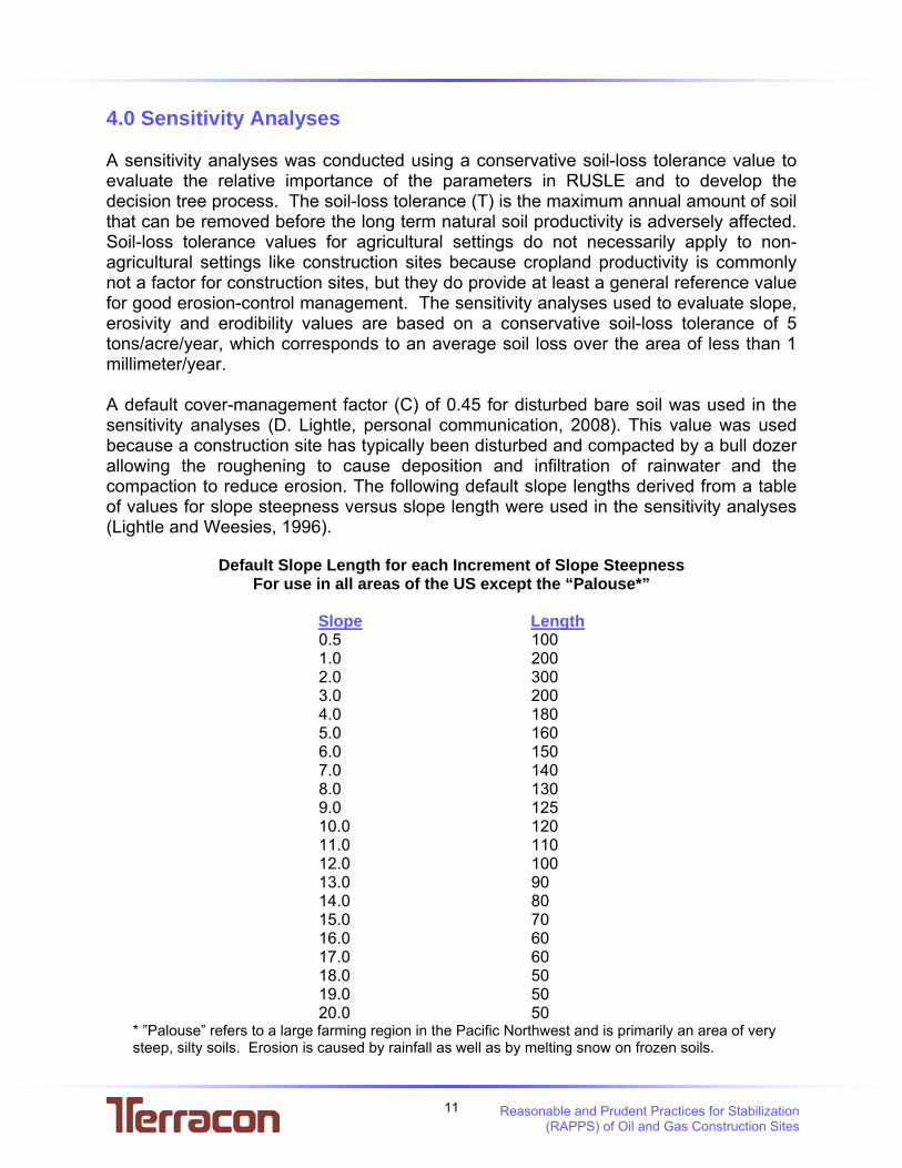
4.0 Sensitivity Analyses A sensitivity analyses was conducted using a conservative soil-loss tolerance value to evaluate the relative importance of the parameters in RUSLE and to develop the decision tree process. The soil-loss tolerance (T) is the maximum annual amount of soil that can be removed before the long term natural soil productivity is adversely affected. Soil-loss tolerance values for agricultural settings do not necessarily apply to non-agricultural settings like construction sites because cropland productivity is commonly not a factor for construction sites, but they do provide at least a general reference value for good erosion-control management. The sensitivity analyses used to evaluate slope, erosivity and erodibility values are based on a conservative soil-loss tolerance of 5 tons/acre/year, which corresponds to an average soil loss over the area of less than 1 millimeter/year. A default cover-management factor (C) of 0.45 for disturbed bare soil was used in the sensitivity analyses (D. Lightle, personal communication, 2008). This value was used because a construction site has typically been disturbed and compacted by a bull dozer allowing the roughening to cause deposition and infiltration of rainwater and the compaction to reduce erosion. The following default slope lengths derived from a table of values for slope steepness versus slope length were used in the sensitivity analyses (Lightle and Weesies, 1996).
Default Slope Length for each Increment of Slope Steepness
For use in all areas of the US except the “Palouse*”
Slope Length 0.5 100 1.0 200 2.0 300 3.0 200 4.0 180 5.0 160 6.0 150 7.0 140 8.0 130 9.0 125 10.0 120 11.0 110 12.0 100 13.0 90 14.0 80 15.0 70 16.0 60 17.0 60 18.0 50 19.0 50 20.0 50
* ”Palouse” refers to a large farming region in the Pacific Northwest and is primarily an area of very steep, silty soils. Erosion is caused by rainfall as well as by melting snow on frozen soils.

12 Reasonable and Prudent Practices for Stabilization (RAPPS) of Oil and Gas Construction Sites
The length-slope (LS) factors were determined using a table developed by the USDA and documented in USDA Agricultural Handbook No. 703 (1997) that lists LS factors for a unique combination of length (ft.) and steepness (%) of the slope. The algorithm used in the table is the same as that used subsequently in RUSLE2. Table 1- LS Values for Construction Sites (Source: USDA Agricultural Handbook No. 703)
Slope Length (ft.) Slope (%)
50 75 100 150 200 250 300 400 0.2 0.05 0.05 0.05 0.05 0.06 0.06 0.06 0.06 0.5 0.08 0.08 0.09 0.09 0.1 0.1 0.1 0.11 1 0.13 0.14 0.15 0.17 0.18 0.19 0.2 0.22 2 0.21 0.25 0.28 0.33 0.37 0.4 0.43 0.48 3 0.3 0.36 0.41 0.5 0.57 0.64 0.69 0.8 4 0.38 0.47 0.55 0.68 0.79 0.89 0.98 1.14 5 0.46 0.58 0.68 0.86 1.02 1.16 1.28 1.51 6 0.54 0.69 0.82 1.05 1.25 1.43 1.6 1.9 8 0.7 0.91 1.1 1.43 1.72 1.99 2.24 2.7
10 0.91 1.2 1.46 1.92 2.34 2.72 3.09 3.75 12 1.15 1.54 1.88 2.51 3.07 3.6 4.09 5.01 14 1.4 1.87 2.31 3.09 3.81 4.48 5.11 6.3 16 1.64 2.21 2.73 3.68 4.56 5.37 6.15 7.6 20 2.1 2.86 3.57 4.85 6.04 7.16 8.23 10.24 25 2.67 3.67 4.59 6.3 7.88 9.38 10.81 13.53 30 3.22 4.44 5.58 7.7 9.67 11.55 13.35 16.77 40 4.24 5.89 7.44 10.35 13.07 15.67 18.17 22.95 50 5.16 7.2 9.13 12.75 16.16 19.42 22.57 28.6 60 5.97 8.37 10.63 14.89 18.92 22.78 26.51 33.67
In the initial sensitivity analyses, the importance of slope in RUSLE was evaluated by plotting slope percent versus rainfall erosivity (R) for various soil types where tolerable soil loss equaled 5 tons/acre/year. The critical slopes were identified by examining the level of convergence between the trend lines.

13 Reasonable and Prudent Practices for Stabilization (RAPPS) of Oil and Gas Construction Sites
Figure 1. R-value vs. Slope for various K values (assuming A = 5 tons/acre/yr) p ( y )
412
130
86
193
61
40
144
4530
0
50
100
150
200
250
300
350
400
450
0.00 1.00 2.00 3.00 4.00 5.00 6.00
Slope (%)
Eros
ivity
(R) v
alue
K=0.15 (Sand)K=0.32 (Clay)K=0.43 (Silt Loam)
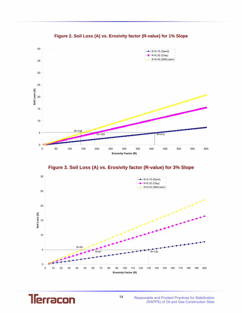
As shown in Figure1, the R values that yield the target A = 5 tons/acre/yr for varying soil types and K values including sand (K=0.15), clay (K=0.32) and silt loam (K=0.43) tend to vary greatly at a slope of 1% and converge at a slope of approximately 3%. The R values further converge at a slope of approximately 5%. This analysis indicates that at sites with slopes steeper than 5%, the soil types begin to behave in a similar fashion. The importance of the erosivity factor in RUSLE was evaluated by plotting erosivity versus soil loss with the above-referenced soil types at slopes of 1%, 3% and 5% (Figures 2, 3, and 4). The following graphs indicate that soil loss increases from sand to clay to silt loam for a given rainfall erosivity (R) value for the different slopes. Figures 2, 3 and 4 indicate the significant R values for each soil type where soil loss equals 5 tons/acre/year at 1%, 3% and 5% slopes used in the decision trees, except for steeper slopes. Steeper slopes (>5%) were also modeled to evaluate their effect on soil loss.
14 Reasonable and Prudent Practices for Stabilization (RAPPS) of Oil and Gas Construction Sites
Figure 2. Soil Loss (A) vs. Erosivity factor (R-value) for 1% Slope
0
5
10
15
20
25
30
35
40
0 50 100 150 200 250 300 350 400 450 500 550 600
Erosivity Factor (R)
Soil
Loss
(A)
K=0.15 (Sand)K=0.32 (Clay)K=0.43 (Silt/Loam)
R=144R=193 R=412
Figure 3. Soil Loss (A) vs. Erosivity factor (R-value) for 3% Slope
0
5
10
15
20
25
30
0 10 20 30 40 50 60 70 80 90 100 110 120 130 140 150 160 170 180 190 200
Erosivity Factor (R)
Soil
Loss
(A)
K=0.15 (Sand)K=0.32 (Clay)K=0.43 (Silt/Loam)
R=45
R=61 R=130
15 Reasonable and Prudent Practices for Stabilization (RAPPS) of Oil and Gas Construction Sites
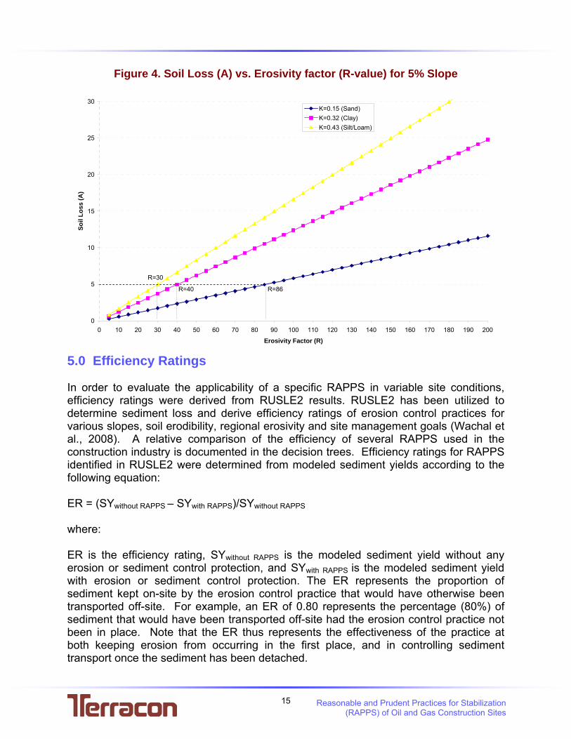
Figure 4. Soil Loss (A) vs. Erosivity factor (R-value) for 5% Slope
0
5
10
15
20
25
30
0 10 20 30 40 50 60 70 80 90 100 110 120 130 140 150 160 170 180 190 200
Erosivity Factor (R)
Soil
Loss
(A)
K=0.15 (Sand)K=0.32 (Clay)K=0.43 (Silt/Loam)
R=30
R=40 R=86
5.0 Efficiency Ratings
In order to evaluate the applicability of a specific RAPPS in variable site conditions, efficiency ratings were derived from RUSLE2 results. RUSLE2 has been utilized to determine sediment loss and derive efficiency ratings of erosion control practices for various slopes, soil erodibility, regional erosivity and site management goals (Wachal et al., 2008). A relative comparison of the efficiency of several RAPPS used in the construction industry is documented in the decision trees. Efficiency ratings for RAPPS identified in RUSLE2 were determined from modeled sediment yields according to the following equation: ER = (SYwithout RAPPS – SYwith RAPPS)/SYwithout RAPPS where: ER is the efficiency rating, SYwithout RAPPS is the modeled sediment yield without any erosion or sediment control protection, and SYwith RAPPS is the modeled sediment yield with erosion or sediment control protection. The ER represents the proportion of sediment kept on-site by the erosion control practice that would have otherwise been transported off-site. For example, an ER of 0.80 represents the percentage (80%) of sediment that would have been transported off-site had the erosion control practice not been in place. Note that the ER thus represents the effectiveness of the practice at both keeping erosion from occurring in the first place, and in controlling sediment transport once the sediment has been detached.

16 Reasonable and Prudent Practices for Stabilization (RAPPS) of Oil and Gas Construction Sites
Wachal et al. (2003) compared efficiency ratings to management goals to evaluate if erosion control methods removed a sufficient amount of sediment for a particular site. The site management goal represents a measure of the acceptable amount of sediment removed by the erosion control method under site-specific conditions. A management goal of 0.60 indicates that an erosion control method must reduce the sediment yield by 60% compared to the sediment yield that would occur if no erosion control methods were in place. In north central Texas, a management goal of 0.70 has been suggested as a minimum guideline to achieve adequate design of erosion and sediment control plans (NCTCOG ISWM Manual, 2003). For example, if selection of a specific RAPPS indicated a site-specific efficiency of 0.75 and the management goal was 0.70, then the goal has been met, and the RAPPS should be sufficient to prevent undesirable quantities of sediment from leaving the construction site assuming RAPPS are designed, constructed and maintained properly. Management goals may vary depending on the sensitivity of the site. For example, the management goal may be set higher for construction near a gold medal trout stream, whereas it may be set lower in an arid, upland, industrial setting. Based on the literature, a general management goal of 0.70 is suggested for construction in non-sensitive areas. Additionally, if the local agency suggests a region-specific management goal, the user should utilize that goal. The county USDA NRCS office or regional council of governments should be contacted to evaluate the region-specific management goal. In low slope conditions (<2%), the efficiencies of practices are mathematically decreased because the sediment yield without RAPPS is lower, and the resultant numerator of the efficiency rating equation is lower. Based on soil loss modeling data, sites with silt/loam and clay soils and low (<2%) slopes exhibit special conditions using this method and it is appropriate to lower the management goal to 0.60 compared to a default management goal of 0.70 for the other decision tree paths. For example, a site with a silt loam soil, a 1% slope, an erosivity > 145, and use of a silt fence results in 1.9 tons/acre/year of soil loss which equates to an efficiency rating of 0.67. However, a similar site with a silt loam, a 5% slope, an erosivity >120, utilizing a sediment basin results in 4.8 tons/acre/year of soil which equates to an efficiency rating of 0.80.
Location Soil Type
Erodibility Value
R Value
Length of Slope (ft.)
Slope (%)
Supporting Practices
Sediment Yield (A,tons/acre/yr)
Efficiency Rating
Texas-Scurry
Silt Loam 0.43 145 200 1 Silt fence 1.9 0.67
Texas-Reagan
Silt Loam 0.43 120 200 5 Sediment Basin 4.8 0.80
Additionally, soil loss modeling data indicated soil loss tolerance levels below 5 tons/acre/year for an efficiency rating of 0.60 with low slopes and silt/loam and clay soils.
17 Reasonable and Prudent Practices for Stabilization (RAPPS) of Oil and Gas Construction Sites
6.0 Using the RAPPS Process 6.1 RUSLE2 Process
This guidance document has been prepared to help operators select various RAPPS based on site specific conditions. The evaluation of RAPPS efficiency ratings is based on the RUSLE2 computer program output. As previously stated the RUSLE 2 computer model was used to develop this guidance document. For more information on it or if a user would like to evaluate their proposed site using the RUSLE2 computer program, it may be downloaded from official RUSLE2 Internet Sites supported by the USDA-ARS at http://www.sedlab.olemiss.edu/RUSLE/, the USDA-Natural Resources Conservation Service (NRCS) at ftp://fargo.nserl.purdue.edu/pub/RUSLE2/ and the University of Tennessee at http://bioengr.ag.utk.edu/RUSLE2/. These internet sites also have supporting information for RUSLE2 including a tutorial, a sample database and a slide set that provides an overview. The RUSLE2 program may be used to evaluate soil loss by entering the site specific factors into the model. A discussion of the use of RUSLE2 is beyond the scope of this document, but more detail is provided in the RUSLE2 user guide, which can be found in its entirety and downloadable PDF at http://fargo.nserl.purdue.edu/rusle2_dataweb/RUSLE2_Technology.htm, and the supporting information in the above-referenced Internet Sites may be used to learn the basic operation of the RUSLE2 computer program. In spite of all this available information and attempts by its developers to make RUSLE2 user-friendly, it is also clear that RUSLE is intended to be used after some training in both the scientific model and user interface. There is currently a pronounced lack of such training besides that provided by USDA-NRCS for its personnel and Technical Support. 6.2 Decision Tree Process
The following RAPPS guidance is an alternative to using the RUSLE2 program and evaluating efficiency ratings from the model’s output results. The RAPPS site evaluation consists of six steps which allow the user to objectively evaluate efficient erosion control(s) for a given set of site conditions. Attachment 1 is a quick reference user guide that is intended to help the user evaluate slope, erosivity and erodibility. The user guide may be copied and laminated for use in the field. Subsequent to the installation of the suggested RAPPS, the effectiveness of the employed RAPPS should be evaluated and modified to reduce soil loss from the site, if necessary. When used correctly, the result will guide the operator to select efficient RAPPS to meet management goals. The RAPPS selection process consists of the following steps:
SStteepp 11)) DDeeffiinnee tthhee ssllooppee ooff tthhee aarreeaa ttoo bbee ddiissttuurrbbeedd;; SStteepp 22)) DDeetteerrmmiinnee tthhee ssiittee aavveerraaggee rraaiinnffaallll eerroossiivviittyy ((RR VVaalluuee));;
SStteepp 33)) DDeetteerrmmiinnee ssooiill ttyyppee ooff aarreeaa ttoo bbee ddiissttuurrbbeedd;; SStteepp 44)) SSeelleecctt oonnee ooff tthhee nniinnee RRAAPPPPSS ddeecciissiioonn ttrreeeess bbaasseedd oonn aann
eevvaalluuaattiioonn ooff ssllooppee aanndd eerroossiivviittyy;;

18 Reasonable and Prudent Practices for Stabilization (RAPPS) of Oil and Gas Construction Sites
SStteepp 55)) SSeelleecctt tthhee aapppprroopprriiaattee ppaatthh ooff tthhee ddeecciissiioonn ttrreeee bbaasseedd oonn ssooiill ttyyppee ttoo eevvaalluuaattee tthhee eeffffiicciieennccyy ooff RRAAPPPPSS;;
SStteepp 66)) CCoommppaarree EERR ttoo MMaannaaggeemmeenntt GGooaall
Subsequent to selection of a RAPPS or a combination of RAPPS, the following sequential tasks should be employed until the construction site is re-vegetated or stabilized:
SStteepp 77)) IInnssttaallll RRAAPPPPSS iinn aapppprroopprriiaattee llooccaattiioonnss bbeeffoorree bbeeggiinnnniinngg cclleeaarriinngg,,
ggrraaddiinngg aanndd eexxccaavvaattiioonn aaccttiivviittiieess..
■ It should be noted that most of the RAPPS combinations were modeled with the RAPPS located near the base of the slope and 75% down the slope.
■ It should be noted that a consensus of erosion control experts and regulatory
agencies recommend preserving existing vegetation and re-establishing vegetation (i.e. seeding, sodding, or hydroseeding) on the disturbed slope as the preferred method of stabilization. Therefore, preserving and re-establishing vegetation should always be encouraged regardless of the particular RAPPS chosen.
SStteepp 88)) BBeeggiinn ssiittee ccoonnssttrruuccttiioonn;; SStteepp 99)) IInnssppeecctt RRAAPPPPSS dduurriinngg oorr ssuubbsseeqquueenntt ttoo aa rraaiinnffaallll eevveenntt aanndd
eevvaalluuaattee iiff sseeddiimmeenntt hhaass bbeeeenn ddeeppoossiitteedd ooffff tthhee ssiittee;; SStteepp 1100)) MMooddiiffyy oorr aadddd RRAAPPPPSS ttoo pprreevveenntt ooffff--ssiittee sseeddiimmeenntt yyiieelldd,, iiff
nneecceessssaarryy;; SStteepp 1111)) CCoommpplleettee ccoonnssttrruuccttiioonn;; SStteepp 1122)) VVeeggeettaattee aanndd//oorr ssttaabbiilliizzee ddiissttuurrbbeedd aarreeaass ffoolllloowwiinngg ccoommpplleettiioonn ooff
ccoonnssttrruuccttiioonn..
6.2.1 DEFINE THE SLOPE OF THE AREA TO BE DISTURBED RAPPS should be installed prior to the construction activity, so the predominant pre-construction slope of the area should be evaluated. If the construction area has more than one definable slope, then the predominant slope where the construction activity is intended should be used. RUSLE2 has the ability to compute sediment yield using a number of different slope profiles. For the purposes of this guidance, a uniform slope profile has been used to model soil loss and to develop the decision trees. The slope of an oil and gas well pad subsequent to construction activities is commonly modified to include a cut and fill slope. The cut slope and toe of the fill slope will typically be steeper than the original slope, and the well pad slope will typically be shallower than the original slope. The preconstruction slope was used because the resultant slope of the well pad is typically shallower, but takes into account the cut slope, the fill slope and slopes in up-gradient and down-gradient positions where water is flowing onto and leaving the construction site as illustrated in Figure 5.

19 Reasonable and Prudent Practices for Stabilization (RAPPS) of Oil and Gas Construction Sites
Figure 5. Use of Pre-construction Slope for Construction Sites
Slope is defined as the amount of elevation gain over a given distance (vertical rise to horizontal run). Slope is determined by measuring the elevation change over a linear distance. The slope percentage is calculated by dividing the elevation change by the linear distance. For example, Figure 5 illustrates a hill with 6 feet of elevation gain over a distance of 200 feet, which represents a 3% slope. A common engineering practice consists of evaluating slope on increments of 100 feet for the purpose of practicality. It should be noted that slope percent and slope angle are not the same, and a table has been included in this section to assist in the conversion from slope angle to percent slope. The elevation change can be determined utilizing several methods including field methods, trigonometric methods, the use of aerial photographs or a site-specific topographic survey, if available. Field methods to determine elevation gain include the use of an altimeter commonly found on GPS units, surveyor’s line-of-sight level, Abney level, a clinometer (also found on a Brunton compass), a digital level, or other surveying equipment (e.g., a total station). The Slope Of The Area To Be Disturbed can be determined using the following equation:
Position Lateral in Difference
Elevation in DifferenceSlope = This is equivalent to: x100
Run
Rise%Slope = x100
ΔX
ΔZ⎟⎠⎞
⎜⎝⎛
=
20 Reasonable and Prudent Practices for Stabilization (RAPPS) of Oil and Gas Construction Sites
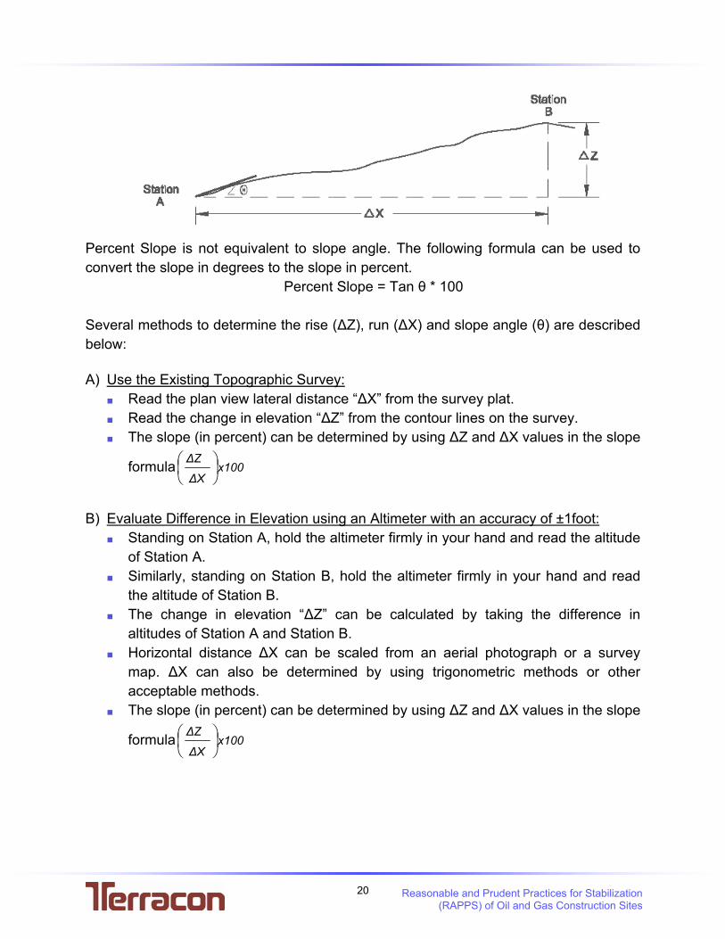
Percent Slope is not equivalent to slope angle. The following formula can be used to convert the slope in degrees to the slope in percent.
Percent Slope = Tan θ * 100 Several methods to determine the rise (ΔZ), run (ΔX) and slope angle (θ) are described below: A) Use the Existing Topographic Survey:
■ Read the plan view lateral distance “ΔX” from the survey plat. ■ Read the change in elevation “ΔZ” from the contour lines on the survey. ■ The slope (in percent) can be determined by using ΔZ and ΔX values in the slope
formula x100ΔX
ΔZ⎟⎠⎞
⎜⎝⎛
B) Evaluate Difference in Elevation using an Altimeter with an accuracy of ±1foot:
■ Standing on Station A, hold the altimeter firmly in your hand and read the altitude of Station A.
■ Similarly, standing on Station B, hold the altimeter firmly in your hand and read the altitude of Station B.
■ The change in elevation “ΔZ” can be calculated by taking the difference in altitudes of Station A and Station B.
■ Horizontal distance ΔX can be scaled from an aerial photograph or a survey map. ΔX can also be determined by using trigonometric methods or other acceptable methods.
■ The slope (in percent) can be determined by using ΔZ and ΔX values in the slope
formula x100ΔX
ΔZ⎟⎠⎞
⎜⎝⎛

21 Reasonable and Prudent Practices for Stabilization (RAPPS) of Oil and Gas Construction Sites
C) Use a GPS unit with elevation capabilities and a resolution of at least 1 sq. ft.: ■ Set the unit to UTM coordinates. ■ Record the coordinates (X1, Y1) and elevation (Z1) at the base of the slope you
wish to measure. ■ Record the elevation (Z2) and coordinates (X2, Y2) at the top of the slope you
wish to measure. ■ The Elevation Rise “ΔZ” = Z2 – Z1
■ The Run Distance “ΔX” = ( )2)1Y2(Y2)1X2(X −+− ■ The slope (in percent) can be determined by using ΔZ and ΔX values in the slope
formula x100ΔX
ΔZ⎟⎠⎞
⎜⎝⎛
D) Use a Digital Level
■ Place the level directly on the surface of the slope. ■ Read the percent slope directly from the instrument.
o It should be noted that this method should only be used for steep slopes.
E) Measure the slope in degrees (θ) and convert to percent slope: ■ Use a Brunton compass (shown below) or Abney level to measure the slope
angle “θ” in degrees.
■ Use the following formula to convert the slope in degrees to the slope in percent: Percent Slope = Tan θ * 100
Using a Brunton compass to measure slope angle
■ It should be noted that this method should only be used for steep slopes. ■ The Tan θ values can be determined using the tangent table as shown below.
Tangent Table
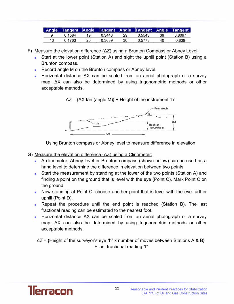
Angle Tangent Angle Tangent Angle Tangent Angle Tangent1 0.0175 11 0.1944 21 0.3838 31 0.6008 2 0.0349 12 0.2125 22 0.404 32 0.6248 3 0.0524 13 0.2309 23 0.4244 33 0.6493 4 0.0699 14 0.2493 24 0.4452 34 0.6744 5 0.0875 15 0.2679 25 0.4663 35 0.7001 6 0.1051 16 0.2867 26 0.4877 36 0.7265 7 0.1228 17 0.3057 27 0.5095 37 0.7535 8 0.1405 18 0.3249 28 0.5317 38 0.7812
22 Reasonable and Prudent Practices for Stabilization (RAPPS) of Oil and Gas Construction Sites
Angle Tangent Angle Tangent Angle Tangent Angle Tangent9 0.1584 19 0.3443 29 0.5543 39 0.8097
10 0.1763 20 0.3639 30 0.5773 40 0.839
F) Measure the elevation difference (ΔZ) using a Brunton Compass or Abney Level: ■ Start at the lower point (Station A) and sight the uphill point (Station B) using a
Brunton compass. ■ Record angle M on the Brunton compass or Abney level. ■ Horizontal distance ΔX can be scaled from an aerial photograph or a survey
map. ΔX can also be determined by using trigonometric methods or other acceptable methods.
ΔZ = {ΔX tan (angle M)} + Height of the instrument “h”
Using Brunton compass or Abney level to measure difference in elevation
G) Measure the elevation difference (ΔZ) using a Clinometer:
■ A clinometer, Abney level or Brunton compass (shown below) can be used as a hand level to determine the difference in elevation between two points.
■ Start the measurement by standing at the lower of the two points (Station A) and finding a point on the ground that is level with the eye (Point C). Mark Point C on the ground.
■ Now standing at Point C, choose another point that is level with the eye further uphill (Point D).
■ Repeat the procedure until the end point is reached (Station B). The last fractional reading can be estimated to the nearest foot.
■ Horizontal distance ΔX can be scaled from an aerial photograph or a survey map. ΔX can also be determined by using trigonometric methods or other acceptable methods.
ΔZ = {Height of the surveyor’s eye “h” x number of moves between Stations A & B}
+ last fractional reading “f”

23 Reasonable and Prudent Practices for Stabilization (RAPPS) of Oil and Gas Construction Sites
Using the Brunton Compass as a Clinometer
Measuring the difference in elevation between two stations by using a hand level and counting eye-level increments
H) Determine the slope angle (θ) using the graphical three-point method:
■ Mark three points (A, B, C) at different elevations on the surface of the preconstruction slope on a site topographic survey, as shown in figure (i) below.
■ Locate Point D on the graph, which is at the same elevation as Point B, on the line joining Points A & C, as shown in figure (ii). Point D can be located by solving the relation:
AD = ACC & APoints Between Elevation in Difference
B & APoints Between Elevation in Difference
■ Level line BD is the direction perpendicular to the steepest slope of the preconstruction slope surface.
■ The slope angle “θ” of the preconstruction slope can be determined by measuring the distance perpendicular to BD, i.e. AE.
■ The slope angle “θ” can be determined from the following equation:
Tan θ = AE Distance
B & APoints Between Elevation in Difference
(i) (ii)
■ The following formula can be used to convert the slope in degrees to the slope in percent.
Percent Slope = Tan θ * 100
24 Reasonable and Prudent Practices for Stabilization (RAPPS) of Oil and Gas Construction Sites
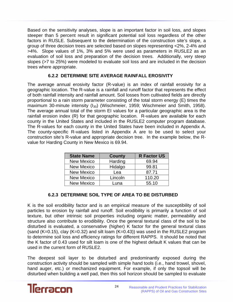
Based on the sensitivity analyses, slope is an important factor in soil loss, and slopes steeper than 5 percent result in significant potential soil loss regardless of the other factors in RUSLE. Subsequent to the determination of the construction site’s slope, a group of three decision trees are selected based on slopes representing <2%, 2-4% and >4%. Slope values of 1%, 3% and 5% were used as parameters in RUSLE2 as an evaluation of soil loss and preparation of the decision trees. Additionally, very steep slopes (>7 to 25%) were modeled to evaluate soil loss and are included in the decision trees where appropriate.
6.2.2 DETERMINE SITE AVERAGE RAINFALL EROSIVITY
The average annual erosivity factor (R-value) is an index of rainfall erosivity for a geographic location. The R-value is a rainfall and runoff factor that represents the effect of both rainfall intensity and rainfall amount. Soil losses from cultivated fields are directly proportional to a rain storm parameter consisting of the total storm energy (E) times the maximum 30-minute intensity (I30) (Wischmeier, 1959; Wischmeier and Smith, 1958). The average annual total of the storm EI values for a particular geographic area is the rainfall erosion index (R) for that geographic location. R-values are available for each county in the United States and included in the RUSLE2 computer program database. The R-values for each county in the United States have been included in Appendix A. The county-specific R-values listed in Appendix A are to be used to select your construction site’s R-value and appropriate decision tree. In the example below, the R-value for Harding County in New Mexico is 69.94.
State Name County R Factor US New Mexico Harding 69.94 New Mexico Hidalgo 99.81 New Mexico Lea 87.71 New Mexico Lincoln 110.20 New Mexico Luna 55.10
6.2.3 DETERMINE SOIL TYPE OF AREA TO BE DISTURBED
K is the soil erodibility factor and is an empirical measure of the susceptibility of soil particles to erosion by rainfall and runoff. Soil erodibility is primarily a function of soil texture, but other intrinsic soil properties including organic matter, permeability and structure also contribute to erodibility. Once the general textural class of the soil to be disturbed is evaluated, a conservative (higher) K factor for the general textural class (sand (K=0.15), clay (K=0.32) and silt loam (K=0.43)) was used in the RUSLE2 program to determine soil loss and efficiency ratings for different RAPPS. It should be noted that the K factor of 0.43 used for silt loam is one of the highest default K values that can be used in the current form of RUSLE2. The deepest soil layer to be disturbed and predominantly exposed during the construction activity should be sampled with simple hand tools (i.e., hand trowel, shovel, hand auger, etc.) or mechanized equipment. For example, if only the topsoil will be disturbed when building a well pad, then this soil horizon should be sampled to evaluate

25 Reasonable and Prudent Practices for Stabilization (RAPPS) of Oil and Gas Construction Sites
the general textural class. However, if the well pad construction involves removing several feet of soil, then the topsoil or subsoil horizon that will have the most area of exposure subsequent to the construction activities should be evaluated. Soil texture represents the relative proportion of silt-, sand-, and clay-sized particles in a soil. This document uses the USDA soil texture classification system, and the USDA soil textural triangle is shown in Figure 6. The mineral particles in the soil are divided into the following size classes: gravel (greater than 2mm), sand (0.05 - 2mm), silt (0.002 - 0.05mm) and clay (smaller than 0.002 mm). The textural triangle specifies 12 different textural classes of soil based on particle-size distribution. The textural class may be determined by evaluating the percentages of any two particle size groupings. Figure 6 has been color coded to illustrate the three general soil textural classifications. The texture of a soil and the associated K factor for a given site may be determined or estimated using several different methods. The K factors for most cropland soils and some rangelands and forestlands may be obtained from USDA-NRCS soil surveys, available at most county NRCS offices. K factors are also included in the Soil Survey Geographic (SSURGO) database (http://soildatamart.nrcs.usda.gov/) and the Web Soil Survey database (http://websoilsurvey.nrcs.usda.gov/app/). These databases allow the user to find their proposed construction site on aerial photographs and evaluate the soil series and associated K factor. A field-method approach may also be used to evaluate the texture of a soil and the associated K factor. This document simplifies the determination of texture and groups the 12 textural classes into three general groups including sand, clay and silt/loam, which are designated by different color codes in the textural triangle (Figure 6). Percentages of clay, silt and sand are also included on Figure 6 for the 12 textural classes grouped into the three general textural classifications. The field-method approach to evaluate soil texture is described in the Soil Texture Decision Chart illustrated in Figure 7. This method will help users classify the soil at their site into one of three general soil textural classes. It should be noted that silt has been grouped with the loams, and its occurrence is rare in nature compared to the other textural classes (Ponte, 2003). The RAPPS decision trees only require the user to determine if the soil is sand, clay or silt/loam. This field method approach to evaluate general soil texture is illustrated with photographs in Figure 8.
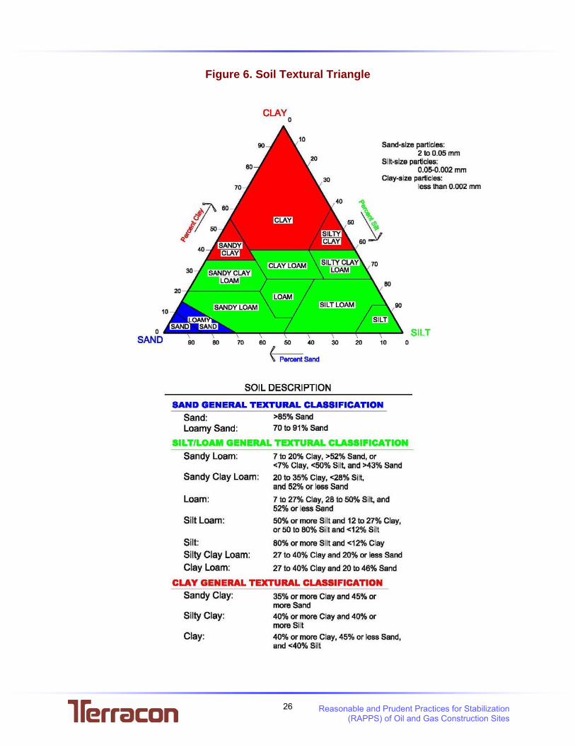
26 Reasonable and Prudent Practices for Stabilization (RAPPS) of Oil and Gas Construction Sites
Figure 6. Soil Textural Triangle

27 Reasonable and Prudent Practices for Stabilization (RAPPS) of Oil and Gas Construction Sites
Figure 7. Soil Texture Decision Chart

28 Reasonable and Prudent Practices for Stabilization (RAPPS) of Oil and Gas Construction Sites
Figure 8. Field Tests to Evaluate Soil Texture
A – Sprinkle a few drops of water on the soil and knead the soil to break down its aggregates
B – Soil is formed into a ball for testing
C – Sand does not remain in a ball when squeezed
D – Loamy Sand does not form a ribbon
E – Less than 2-inch ribbon formed before breaking due to silt/loam content
F – 2-inch ribbon formed due to higher clay content

29 Reasonable and Prudent Practices for Stabilization (RAPPS) of Oil and Gas Construction Sites
6.2.4 SELECTION OF RAPPS USING DECISION TREES Based on an evaluation of slope and erosivity, one of the nine RAPPS decision trees included in Appendix B is selected. Subsequent to evaluation of the soil type, the appropriate path of the decision tree is selected and resultant efficiencies of RAPPS are listed in order of highest to lowest efficiency as shown in Figure 9, which is an example of a RAPPS Decision Tree. If the efficiency of a specific RAPPS exceeds the management goal, then the RAPPS is effective in reducing sediment yield from the site, assuming the RAPPS are designed, operated and maintained properly.
The list of RAPPS provided in Appendix C and D are not exhaustive lists of available erosion control measures, rather they are presentations of the currently popular, cost-effective, efficient erosion control practices used in the U.S. construction market and documented in the construction version of RUSLE2. The examples of RAPPS presented in Appendix C and D are not engineering plans and specifications as defined by ASTM International or the American National Standards Institute (ANSI) and should only be used as a general guide for practices being used in the U.S. marketplace. In some situations, operators may want to consider retaining a certified professional in erosion and sediment control (CPESC) to design RAPPS, inspect constructed RAPPS and provide periodic inspection of the site during operations. A few RAPPS documented in Appendix C (e.g., surface roughening, RGHN) were not included in RUSLE2, and corresponding efficiency ratings were not calculated.
Figure 9. Example of RAPPS Decision Tree

30 Reasonable and Prudent Practices for Stabilization (RAPPS) of Oil and Gas Construction Sites
The RAPPS listed in the decision trees represent the majority of the options in the RUSLE2 computer program for construction sites. A few erosion control methods in RUSLE2 have several variations, and this guidance document typically evaluates the most cost-effective and prevalent erosion control method currently available. For example, three variations of erosion control blankets including rolled material, rolled material with quick decay and rolled material with single net straw may be evaluated with RUSLE2 model; however, the generic erosion control blanket was used to model erosion control blankets because of its common use in the construction industry. Each decision tree path includes a list of RAPPS (abbreviated) and its corresponding efficiency rating listed in order of highest to lowest efficiency. If the RAPPS efficiency does not meet the default management goal, then additional combinations of RAPPS with corresponding efficiencies are listed in the decision tree. Figure 9 is an example Decision Tree that illustrates RAPPS nomenclature (CS 0.68) (2CS 0.72), which indicates that a compost sock exhibits an efficiency of 68%, and a combination of two compost socks exhibit an efficiency of 72%. Figure 9 also illustrates RAPPS nomenclature (SF 0.56) (SF/SBB 0.72) which indicates that a silt fence exhibits an efficiency of 56% and a combination of a silt fence with a straw bale barrier exhibits an efficiency of 72%. If a combination of specific RAPPS did not meet a management goal of 70%, then the RAPPS combination was not listed in the decision trees. The combinations of RAPPS that were selected are not an exhaustive list of RAPPS combinations, but represent a number of RAPPS that are efficient, economical, commonly used and/or relatively easy to install that meet the default management goal of at least 70%. It should be noted that most of the RAPPS combinations were modeled with the RAPPS located near the base of the slope and 75% down the slope.
6.2.5 SUPPLEMENTAL RAPPS
Under certain circumstances, such as steep slopes or a region with high erosivity (R-values), alternate or additional RAPPS should be employed to prevent discharges of potentially undesirable quantities of sediment. In those cases, one or a combination of two RAPPS documented in the decision trees will not provide adequate protection above a specified slope, R-Value or combination of slope and R-value. This specific situation is noted in the soil type decision box in the decision tree paths. The RAPPS used for these situations are referred to as “Supplemental RAPPS” and are expected to achieve the intent of the efficiency goal as a combined system of RAPPS. Supplemental RAPPS are a combination of two or more listed RAPPS or Specialty RAPPS and are required if a site has high risk attributes that exceed the values prescribed in the decision trees (Appendix B – Decision trees 3, 6, 7, 8 & 9). Supplemental RAPPS were employed in situations where soil loss modeling data consistently indicated that an efficiency rating of 70% could not be achieved with a combination of at least two RAPPS, or potential undesirable quantities of sediment may be transported off the site even while meeting the management goal. Installation and maintenance of these Supplemental RAPPS in accordance with accepted construction practices using good judgment should provide adequate erosion and sediment control. However, other combinations of RAPPS in site-specific conditions using good judgment

31 Reasonable and Prudent Practices for Stabilization (RAPPS) of Oil and Gas Construction Sites
should be employed, if necessary. It should be noted that a consensus of erosion control experts and regulatory agencies recommend preserving existing vegetation and re-establishing vegetation (i.e. seeding, sodding, or hydroseeding) on the disturbed slope as the preferred method of stabilization. Therefore, preserving and re-establishing vegetation should always be encouraged regardless of the particular RAPPS chosen. In the case of a site with a steep pre-construction slope (Decision Trees 7, 8 & 9), the user should employ Supplemental RAPPS that will: 1) reduce the amount of stormwater reaching the site by redirecting the up-gradient run-on flow of stormwater around the construction site by means of a diversion structure (i.e., a diversion dike, interceptor swale, ditches, slope drains); 2) protect disturbed soil on the slope with a form of cover (i.e., mulch and/or erosion control mat); and 3) protect the base of the slope with a runoff-velocity barrier (i.e., rock berm, compost sock, brush piles, fiber rolls/logs). It should be noted that soil loss modeling data indicate that silt fences and straw hay bales should not be used at the bottom of steep slopes as they do not function well in high runoff-velocity conditions. In the case of a site with a high Erosivity (R value - Decision Trees 3, 6 or 9), the user should employ Supplemental RAPPS that will: 1) protect disturbed soil on the slope with roughening and a form of cover (i.e., mulch, straw, compost and/or erosion control mat); and 2) protect the base of the slope with runoff-velocity barriers (i.e., silt fence, straw bales, fiber rolls/logs, rock berms, vegetative barrier or brush piles). In the case of a construction site adjacent to a drainage feature or a water way, the use of sediment basins or other sediment capturing containment structures (i.e. silt trap, dewatering structure, filter bag) are recommended. The above-referenced scenarios are not an exhaustive list of the site-specific situations that could be encountered during oil and gas construction activity. It should be noted that other combinations of RAPPS in site specific situations should be installed using good judgment, if required to prevent undesirable quantities of sediment being transported off the site. If these situations exist, operators may want to consider retaining a CPESC to design RAPPS, inspect constructed RAPPS and provide periodic inspection of the site during operations.
6.2.6 OPERATIONAL RAPPS
Under certain circumstances including a combination of low slopes, low R-values and/or low to moderate K-values, implementation of RAPPS beyond Operational RAPPS may not be required. Construction sites with modeled low soil loss (<5 tons/acre/year) using conservative input values including a C factor of 1.0 in the RUSLE2 program require Operational RAPPS. Operational RAPPS reflect a minimal effort of erosion control including installation of an inexpensive sediment barrier (i.e., compost sock, compost berm, vegetative barrier, brush pile, interceptor swale, soil berm, straw bale barriers or silt fence) near the downgradient boundary of the construction site along with the following practices that operators are commonly using as part of normal operations:

32 Reasonable and Prudent Practices for Stabilization (RAPPS) of Oil and Gas Construction Sites
■ Planning the site location to choose low-slope sites away from waterways;
■ Minimizing the footprint of the disturbed area; ■ Phasing/scheduling projects to minimize soil disturbance; ■ Timing the project during dry weather periods of the year; ■ Managing slopes to decrease steepness; ■ Maintaining the maximum amount of vegetative cover as possible; ■ Cutting vegetation above ground level and limiting removal of
vegetation, root zones and stumps, where possible; ■ Limiting site disturbance to only clear what is necessary; ■ Practicing good housekeeping including proper material storage;
and ■ Practicing operation and maintenance procedures to limit sediment
yield (i.e. maintaining silt fence). 6.2.7 SPECIALTY RAPPS
During construction of oil and gas sites, an operator may encounter special circumstances including crossing a regulated water body or construction near a roadway that require Specialty RAPPS to divert or reduce the velocity of surface water flow. Specialty RAPPS near roadways are also constructed to limit the amount of sediment leaving the site via truck traffic. Specialty RAPPS are not included in RUSLE2 because they are not considered general erosion control practices to reduce sediment yield and are used in special circumstances. Efficiency ratings for Specialty RAPPS were not calculated in this document because their corresponding P factors are not included in RUSLE2. Specialty RAPPS are documented in Appendix D and include Stabilized Construction Entrance (SCE), Road Surface Slope (RDSS), Drainage Dips (DIP), Road-Side Ditches (RDSD), Turnouts or Wing Ditches (TO), Cross-drain Culverts (CULV), Sediment Traps (ST), Construction Mats (CM), Filter Bags (FB),Trench Dewatering and Discharge (TDD), Dewatering Structure (DS), Stream Crossing Flume Pipe (SCFP), Stream Crossing Dam and Pump (SCDP), Stream Bank Stabilization (SBS), Dry Stream Crossing (DSC) and the Temporary Equipment Crossing of Flowing Creek (TECFC). Information regarding installation, inspection and maintenance of Specialty RAPPS are included in Appendix D.
33 Reasonable and Prudent Practices for Stabilization (RAPPS) of Oil and Gas Construction Sites
7.0 Final Stabilization RAPPS should be maintained in good condition for the area disturbed during and after the period of active disturbance until final stabilization of the area. Final stabilization will limit and/or prevent potentially undesirable quantities of sediment from leaving the site in storm water runoff and entering a water body. Final stabilization can be achieved by several different methods including stabilization of the road, well pad, and equipment pad, as well as re-vegetation of the native background vegetative cover for the area. After construction of roads and well/equipment pads are completed, the area covered by the road and/or equipment pad is considered stabilized by placing base material on these areas, such as asphalt, cement treated base, aggregate, crushed limestone or other types rock. Once the base material is sufficiently compacted for its intended use, it is considered stabilized. Accepted erosion control guidance typically defines final stabilization as a uniform, (e.g. evenly distributed, without large bare areas) perennial vegetation cover with a density of 70% of the native background vegetation cover for the area has been established on all unpaved areas and areas not covered by permanent structures, or equivalent permanent stabilization measures (such as the use of stabilized construction entrances, rock berms, geotextiles) have been employed. Additionally, erosion control guidance typically requires that temporary erosion control measures are selected, designed, and installed to achieve 70 percent vegetative coverage within three years. This document suggests a re-vegetation goal of 70% as a benchmark to allow oil and gas operators to remove or cease maintenance of erosion control practices. Although a re-vegetation goal of approximately 70% is suggested, federal, state or local regulations may require a specific stabilization goal, and these regulations or guidance documents should be evaluated prior to removal or cessation of maintenance of RAPPS.

34 Reasonable and Prudent Practices for Stabilization (RAPPS) of Oil and Gas Construction Sites
8.0 References
Carleton College, Northfield Minnesota, 2008, Seven-Mile Creek Watershed Project http://www.carleton.edu/departments/GEOL/Links/AlumContributions/Antinoro
_03/SMCwebsite/DrainageSolutions.htm California Straw Works, 5531 State Ave, Sacramento, California 95819. 2008,
http://www.publicworks.com/storefronts/califstraw.html Fifield, J.S., 2005. Best Management Practices for Contractors and Inspectors – Field
Manual on Sediment and Erosion Control. Pp. 56, 92. Foster, G.R., Yoder, D.C., Weesies, G.A., McCool, D.K., McGregor, K.C., Bingner, R.L.,
2003. RUSLE 2.0 User's Guide. USDA-Agricultural Research Service, Washington DC.
Foster, G.R. 2004. Draft User's Reference Guide. Undergoing review: currently
available in draft form at: www.ars.usda.gov/Research/docs.htm?docid=6028. (10 February 2007).
Foster, G.R. 2005. Draft Science Documentation for RUSLE2. Undergoing review:
currently available in draft form at: www.ars.usda.gov/Research/docs.htm?docid=6028. (10 February 2007).
Lightle, Dave. <[email protected]> “SLOPE document”. Personal Communication. (September, 2008).
Ponte, K.J. 2003. Retaining Soil Moisture in the American Southwest. North Central Texas Council of Governments – Construction BMP Manual. 1998 North Central Texas Council of Governments – Integrated Storm Water Management.
Design Manual for Construction. 2003 North American Green Erosion Control, 2006, 14649 Highway 41 North
Evansville, IN 47725. http://www.nagreen.com Ohio Department of Transportation, 2008, http://www.dot.state.oh.us/pages/homes.aspx Pennsylvania Department of Environmental Protection – Chapter 4, Oil and Gas
Management Practices. http://www.dep.state.pa.us/eps/default.asp?P=fldr200149e0051190%5Cfldr200149e10561a8%5Cfldr20026f8082801d (12 February 2004).
Renard, K.G., G.R. Foster, D.K. McCool, and D.C. Yoder, coordinators. 1997.
Predicting Soil Erosion by Water: A Guide to Conservation Planning with the
35 Reasonable and Prudent Practices for Stabilization (RAPPS) of Oil and Gas Construction Sites
Revised Universal Soil Loss Equation (RUSLE). Agriculture Handbook 703. Washington, D.C.: USDA.
University of Tennessee Biosystems Engineering & Soil Science Department,
http://bioengr.ag.utk.edu/RUSLE2/ (5 November, 2008) US Department of Agriculture – Agricultural Research Service. 2008a. Draft User's
Reference Guide. Available at: www.ars.usda.gov/Research/docs.htm?docid=6028. (11 November, 2008). US Department of Agriculture – Agricultural Research Service. 2008b. Draft Science
Documentation for RUSLE2. Available at: www.ars.usda.gov/Research/docs.htm?docid=6028. (11 November, 2008). US Department of Agriculture – Agricultural Research Service. Agricultural Handbook.
Predicting Soil Erosion by Water: A Guide to Conservation Planning With the Revised Universal Soil Loss Equation (RUSLE). No. 703. 1997
US Department of Agriculture – Agricultural Research Service http://www.sedlab.olemiss.edu/RUSLE/ (5 November, 2008)
US Department of Agriculture – Natural Resources Conservation Service ftp://fargo.nserl.purdue.edu/pub/RUSLE2/ (5 November, 2008)
US Department of Agriculture – Natural Resources Conservation Service. RUSLE2 User’s Guide. http://fargo.nserl.purdue.edu/rusle2_dataweb/RUSLE2_Technology.htm (5 November, 2008)
US Department of Agriculture – Natural Resources Conservation Service, Soil Survey Geographic Database. http://soildatamart.nrcs.usda.gov/ (5 November, 2008)
US Department of Agriculture – Natural Resources Conservation Service, Web Soil Survey Database. http://websoilsurvey.nrcs.usda.gov/app/ (5 November, 2008)
US Environmental Protection Agency – National Pollutant Discharge Elimination System (NPDES). Construction Site Storm Water Runoff Control. http://cfpub.epa.gov/npdes/stormwater/menuofbmps/con_site.cfm (12 February 2004).
Virginia Department of Conservation and Recreation, Virginia Erosion and Sediment
Control Handbook, 3rd Edition, 1992

36 Reasonable and Prudent Practices for Stabilization (RAPPS) of Oil and Gas Construction Sites
Wachal, D.J., Banks, K.E., Hudak, P.F., Harmel, R.D. 2008. Modeling Erosion and Sediment Control Practices With RUSLE 2.0: A Management Approach for Natural Gas Well Sites in Denton County, TX, USA.
Wachal, D.J., Banks, K.E. 2006. Modeling and Monitoring Storm Water Impacts from
Natural Gas Well Development Activities. In: Presented at StormCon: The North American Surface Water Quality Conference, Denver CO, July 2006.
Wachal, D.J., Banks, K.E., Hunter, D.H. 2005. Collecting Storm Water from Overland
Flow at gas Exploration and production Sites. In: Presented at Water Environment Federation 78th Annual Conference, Washington DC, October 2005.
Wachal, D.J., Banks, K.E. 2007. Integrating GIS and Erosion Modeling: A Tool for
Watershed Management. ESRI 2007 International User Conference – Paper No. UC1038.
Wachal, D.J., Banks, K.E. 2007. The Application of WEPP to Natural Gas Exploration
and Production Sites. Wachal, D.J., Banks, K.E. 2007. Modeling Erosion and Sediment Control Practices: A
Management Approach for Disturbed Sites. Wischmeier, W.H., D.D. Smith. 1978. Predicting Rainfall Erosion Losses: A Guide to
Conservation Planning. USDA, Agricultural Handbook No. 537. Yoder, D.C., J.S. Tyner, J.D. Balousek, J.C. Panuska, J.R. Buchanan, K.J. Kirsch, and
J.P. Lyon. 2007. Conservation planning for construction sites. Trans. ASABE. 50(5): 1613-1618 .

AT-1
ATTACHMENT 1. RAPPS QUICK REFERENCE USER GUIDE

AT-2
RAPPS QUICK REFERENCE GUIDE Step 1) Determine The Slope Of The Area To Be Disturbed
Position Lateral in Difference
Elevation in DifferenceSlope = This is equivalent to: x100
Run
Rise%Slope = x100
ΔX
ΔZ⎟⎠⎞
⎜⎝⎛
=
Percent Slope is not equivalent to slope angle. The following formula can be used to convert the slope in degrees to the slope in percent.
Percent Slope = Tan θ * 100 The user may choose to evaluate the slope by their own method. However, several methods to determine the rise (ΔZ), run (ΔX) and slope angle (θ) are described in the main text of the RAPPS document Section 6.2.1 (Page 18). Step 2) Determine Site Average Rainfall Erosivity The average annual erosivity factor (R-value) is an index of rainfall erosivity for a geographic location. The R-value is a rainfall and runoff factor that represents the effect of both rainfall intensity and rainfall amount. The R-values for each county in the United States have been included in Appendix A. The county-specific R-values listed in Appendix A are to be used to select your construction site’s R-value. In the example below, the R-value for Harding County in New Mexico is 69.94.
State Name County R Factor US New Mexico Harding 69.94 New Mexico Hidalgo 99.81 New Mexico Lea 87.71 New Mexico Lincoln 110.20
Step 3) Site Erodibility - Determine Soil Type Of Area To Be Disturbed A) Use existing soil surveys located at your local USDA/ Natural Resource Conservation Service (NRCS) office OR
B) Look-up the soil type from the following online Soil Survey Geographic (SSURGO) database or the NRCS
database links:
http://soildatamart.nrcs.usda.gov/ http://websoilsurvey.nrcs.usda.gov/app/
OR C) Use the Soil Texture Decision Chart:
Use the Soil Texture Decision Chart, at the end of Attachment 1, and follow the steps below to determine the predominate soil type to be disturbed at your site (i.e. clay, sand, or silt/loam).

AT-3
Step 4) Select one of the nine RAPPS decision trees based on an evaluation of slope and
erosivity. Step 5) Select the appropriate path of the decision tree based on soil type to evaluate the
efficiency of RAPPS. Each decision tree path includes a list of RAPPS (abbreviated) and its corresponding efficiency rating listed in order of highest to lowest efficiency. The efficiency rating (ER) represents the proportion of sediment kept on-site by the erosion control practice that would have otherwise been transported off-site. For example, an ER of 0.80 represents the percentage (80%) of sediment that would have been transported off-site had the erosion control practice not been in place. Example Decision Tree-5 illustrates RAPPS nomenclature (CS 0.68) (2CS 0.72), which indicates that a compost sock exhibits an efficiency of 68%, and a combination of two compost socks exhibit an efficiency of 72%. Example Decision Tree-5 also illustrates RAPPS nomenclature (SF 0.56) (SF/SBB 0.72) which indicates that a silt fence exhibits an efficiency of 56% and a combination of a silt fence with a straw bale barrier exhibits an efficiency of 72%. A detailed discussion of efficiency ratings is provided in Section 5.0 (Page 15).
Example of RAPPS Decision Tree
Step 6) Compare ER to Management Goal Compare each RAPPS ER for the appropriate soil type path to management goals to evaluate if erosion control methods removed a sufficient amount of sediment for a particular site. The site management goal represents a measure of the acceptable amount of sediment removed by the erosion control method under site-specific conditions. A management goal of 0.60 indicates that an erosion control method must reduce the sediment yield by 60% compared to the sediment yield that would occur if no erosion control methods were in place. Sediment yield is the amount of eroded soil. In north central Texas, a management goal of 0.70 has been suggested as a

AT-4
minimum guideline to achieve adequate design of erosion and sediment control plans (NCTCOG ISWM Manual, 2003). For example, if selection of a specific RAPPS indicated a site-specific efficiency of 0.75 and the management goal was 0.70, then the goal has been met, and the RAPPS should be sufficient to prevent undesirable quantities of sediment from leaving the construction site assuming RAPPS are designed, constructed and maintained properly. If the RAPPS efficiency does not meet the default management goal of 70%, then additional combinations of RAPPS with corresponding efficiencies are listed in the decision tree. Management goals may vary depending on the sensitivity of the site. Based on the literature, a general management goal of 0.70 is suggested for construction in non-sensitive areas. However, if the local agency suggests a region-specific management goal, the user should utilize that goal. The county USDA NRCS office or regional council of governments should be contacted to evaluate the region-specific management goal. Based on soil loss modeling data, sites with silt/loam and clay soils and low (<2%) slopes exhibit special conditions using this method and it is appropriate to lower the management goal to 0.60 compared to a default management goal of 0.70 for the other decision tree paths. A detailed discussion of management goal selection is provided in Section 5.0 (Page 16). In addition to RAPPS documented in the decision trees, other types of RAPPS including Supplemental RAPPS, Operational RAPPS and Specialty RAPPS are discussed below.
Supplemental RAPPS
Under certain circumstances, such as steep slopes or a region with high erosivity (R-values), alternate or additional RAPPS should be employed to prevent discharges of potentially undesirable quantities of sediment. In those cases, one or a combination of two RAPPS documented in the decision trees will not provide adequate protection above a specified slope, R-Value or combination of slope and R-value. This specific situation is noted in the soil type decision box in the decision tree paths. The RAPPS used for these situations are referred to as “Supplemental RAPPS” and are expected to achieve the intent of the efficiency goal as a combined system of RAPPS. Supplemental RAPPS are a combination of two or more listed RAPPS or Specialty RAPPS and are required if a site has high risk attributes that exceed the values prescribed in the decision trees (Appendix B – Decision trees 3, 6, 7, 8 & 9). A detailed discussion on Supplemental RAPPS is provided in Section 6.2.5 (Page 30).
• In the case of a site with a steep pre-construction slope (Decision Trees 7, 8 & 9), the user should employ Supplemental RAPPS that will:
1) reduce the amount of stormwater reaching the site by redirecting the up-gradient run-on flow of
stormwater around the construction site by means of a diversion structure (i.e., a diversion dike, interceptor swale, ditches, slope drains);
2) protect disturbed soil on the slope with a form of cover (i.e., mulch and/or erosion control mat); and 3) protect the base of the slope with a runoff-velocity barrier (i.e., rock berm, compost sock, brush piles,
fiber rolls/logs). It should be noted that soil loss modeling data indicate that silt fences and straw hay bales should not be used at the bottom of steep slopes as they do not function well in high runoff-velocity conditions.
• In the case of a site with a high Erosivity (R value - Decision Trees 3, 6 or 9), the user should employ
Supplemental RAPPS that will:
1) protect disturbed soil on the slope with roughening and a form of cover (i.e., mulch, straw, compost and/or erosion control mat); and
2) protect the base of the slope with runoff-velocity barriers (i.e., silt fence, straw bales, fiber rolls/logs, rock berms, vegetative barrier or brush piles).
• In the case of a construction site adjacent to a drainage feature or a water way, the use of sediment
basins or other sediment capturing containment structures (i.e. silt trap, dewatering structure, filter bag) are recommended.
The above-referenced scenarios are not an exhaustive list of the site-specific situations that could be encountered during oil and gas construction activity. It should be noted that other combinations of RAPPS in site specific situations should be installed using good judgment, if required to prevent undesirable quantities of sediment being transported off the site. If these situations exist, operators may want to consider retaining a certified professional

AT-5
in erosion and sediment control (CPESC) to design RAPPS, inspect constructed RAPPS and provide periodic inspection of the site during operations.
Operational RAPPS
Under certain circumstances including low slopes and/or low erosivity, a minimal erosion control effort may be utilized. Operational RAPPS reflect a minimal effort of erosion control including installation of an inexpensive sediment barrier (i.e., compost sock, compost berm, vegetative barrier, brush pile, interceptor swale, soil berm, straw bale barriers or silt fence) near the downgradient boundary of the construction site along with the following practices that operators are commonly using as part of normal operations: • Planning the site location to choose low-slope sites away from waterways; • Minimizing the footprint of the disturbed area; • Phasing/scheduling projects to minimize soil disturbance; • Timing the project during dry weather periods of the year; • Managing slopes to decrease steepness; • Maintaining the maximum amount of vegetative cover as possible; • Cutting vegetation above ground level and limiting removal of vegetation, root zones and stumps, where
possible; • Limiting site disturbance to only clear what is necessary; • Practicing good housekeeping including proper material storage and • Practicing operation and maintenance procedures to limit sediment yield (i.e. maintaining silt fence).
Specialty RAPPS
During construction of oil and gas sites, an operator may encounter special circumstances including crossing a regulated water body or construction near a roadway that requires Specialty RAPPS to divert or reduce the velocity of surface water flow. Specialty RAPPS near roadways are also constructed to limit the amount of sediment leaving the site via truck traffic. Site-specific conditions should be considered in conjunction with federal, state or local regulatory requirements to ensure that RAPPS are implemented to achieve regulatory compliance, if necessary. Specialty RAPPS are documented in Appendix D and include: • Stabilized Construction Entrance (SCE); • Road Surface Slope (RDSS); • Drainage Dips (DIP); • Road-Side Ditches (RDSD); • Turnouts or Wing Ditches (TO); • Cross-drain Culverts (CULV); • Sediment Traps (ST); • Construction Mats (CM); • Filter Bags (FB); • Trench Dewatering and Discharge (TDD); • Dewatering Structure (DS); • Stream Crossing Flume Pipe (SCFP); • Stream Crossing Dam and Pump (SCDP); • Stream Bank Stabilization (SBS); • Dry Stream Crossing (DSC) and • Temporary Equipment Crossing of Flowing Creek (TECFC). Subsequent to selection of a RAPPS or a combination of RAPPS, the following sequential tasks should be employed until the construction site is re-vegetated or stabilized: Step 7) Install RAPPS in appropriate locations before beginning clearing, grading and
excavation activities.
• It should be noted that most of the RAPPS combinations were modeled with the RAPPS located near the base of the slope and 75% down the slope.
AT-6
• It should be noted that a consensus of erosion control experts and regulatory agencies recommend preserving existing vegetation and re-establishing vegetation (i.e. seeding, sodding, or hydroseeding) on the disturbed slope as the preferred method of stabilization. Therefore, preserving and re-establishing vegetation should always be encouraged regardless of the particular RAPPS chosen.
Step 8) Begin site construction; Step 9) Inspect RAPPS during or subsequent to a rainfall event and evaluate if sediment
has been deposited off the site; Step 10) Modify or add RAPPS to prevent off-site sediment yield, if necessary; Step 11) Complete construction; Step 12) Vegetate and/or stabilize disturbed areas following completion of construction.

AT-7
Soil Texture Decision Chart

AT-8
Field Tests to Evaluate Soil Texture
A – Sprinkle a few drops of water on the soil and knead the soil to break down its aggregates
B – Soil is formed into a ball for testing
C – Sand does not remain in a ball when squeezed
D – Loamy Sand does not form a ribbon
E – Less than 2-inch ribbon formed before breaking due to silt/loam content
F – 2-inch ribbon formed due to higher clay content

A-1
APPENDIX A. EROSIVITY (R-VALUE) TABLES

APPENDIX A. EROSIVITY (R-VALUE TABLES)
State Name County Name R Factor US State Name County R Factor USALABAMA ALABAMA
Alabama Autauga 416.86 Alabama Montgomery 435.61Alabama Baldwin 668.30 Alabama Morgan 362.14Alabama Barbour 429.05 Alabama Perry 430.07Alabama Bibb 423.50 Alabama Pickens 418.79Alabama Blount 364.96 Alabama Pike 453.94Alabama Bullock 422.21 Alabama Randolph 362.40Alabama Butler 475.04 Alabama Russell 388.24Alabama Calhoun 338.38 Alabama St. Clair 370.15Alabama Chambers 392.93 Alabama Shelby 390.83Alabama Cherokee 337.99 Alabama Sumter 444.54Alabama Chilton 411.78 Alabama Talladega 380.46Alabama Choctaw 503.55 Alabama Tallapoosa 410.56Alabama Clarke 539.06 Alabama Tuscaloosa 412.57Alabama Clay 394.00 Alabama Walker 393.34Alabama Cleburne 354.70 Alabama Washington 577.31Alabama Coffee 531.18 Alabama Wilcox 480.62Alabama Colbert 373.57 Alabama Winston 391.61Alabama Conecuh 567.69 ARKANSASAlabama Coosa 407.98 Arkansas Arkansas 357.31Alabama Covington 547.34 Arkansas Ashley 425.18Alabama Crenshaw 496.98 Arkansas Baxter 264.44Alabama Cullman 372.27 Arkansas Benton 284.49Alabama Dale 499.78 Arkansas Boone 274.94Alabama Dallas 434.72 Arkansas Bradley 413.00Alabama De Kalb 343.49 Arkansas Calhoun 394.04Alabama Elmore 410.44 Arkansas Carroll 263.87Alabama Escambia 613.36 Arkansas Chicot 405.46Alabama Etowah 337.73 Arkansas Clark 389.54Alabama Fayette 433.70 Arkansas Clay 286.64Alabama Franklin 391.58 Arkansas Cleburne 325.36Alabama Geneva 543.36 Arkansas Cleveland 388.25Alabama Greene 411.99 Arkansas Columbia 400.20Alabama Hale 419.53 Arkansas Conway 319.22Alabama Henry 463.34 Arkansas Craighead 300.37Alabama Houston 520.13 Arkansas Crawford 312.32Alabama Jackson 332.18 Arkansas Crittenden 337.70Alabama Jefferson 380.78 Arkansas Cross 323.20Alabama Lamar 420.03 Arkansas Dallas 384.01Alabama Lauderdale 363.18 Arkansas Desha 382.09Alabama Lawrence 368.51 Arkansas Drew 399.03Alabama Lee 402.79 Arkansas Faulkner 331.63Alabama Limestone 347.76 Arkansas Franklin 300.94Alabama Lowndes 442.41 Arkansas Fulton 268.73Alabama Macon 416.53 Arkansas Garland 392.70Alabama Madison 339.73 Arkansas Grant 371.52Alabama Marengo 454.52 Arkansas Greene 297.44Alabama Marion 417.90 Arkansas Hempstead 397.31Alabama Marshall 337.60 Arkansas Hot Spring 393.02Arkansas Izard 279.02 Arkansas Howard 397.24Arkansas Jackson 311.26 Arkansas Independence 308.53
A-1

APPENDIX A. EROSIVITY (R-VALUE TABLES)
State Name County R Factor US State Name County R Factor USARKANSAS ARIZONA
Arkansas Jefferson 361.80 Arizona Mohave 38.01Arkansas Johnson 307.56 Arizona Navajo 74.97Arkansas Lafayette 390.52 Arizona Pima 118.70Arkansas Lawrence 289.27 Arizona Pinal 122.43Arkansas Lee 351.47 Arizona SantaCruz 153.64Arkansas Lincoln 380.84 Arizona Yavapai 79.49Arkansas Little River 375.51 Arizona Yuma 28.08Arkansas Logan 315.18 CALIFORNIAArkansas Lonoke 334.77 California Alameda 78.90Arkansas Madison 296.57 California Alpine 162.98Arkansas Marion 269.28 California Amador 118.79Arkansas Miller 372.01 California Butte 208.84Arkansas Mississippi 309.94 California Calaveras 121.84Arkansas Monroe 347.85 California Colusa 157.67Arkansas Montgomery 393.61 California ContraCosta 66.73Arkansas Nevada 398.34 California DelNorte 307.26Arkansas Newton 300.01 California El dorado 153.53Arkansas Ouachita 391.35 California Fresno 115.48Arkansas Perry 350.43 California Glenn 183.66Arkansas Phillips 370.22 California Humboldt 226.26Arkansas Pike 410.15 California Imperial 50.86Arkansas Poinsett 311.13 California Inyo 80.64Arkansas Polk 406.86 California Kern 80.20Arkansas Pope 315.25 California Kings 50.46Arkansas Prairie 339.11 California Lake 146.38Arkansas Pulaski 343.04 California Lassen 86.80Arkansas Randolph 284.47 California LosAngeles 129.77Arkansas St. Francis 339.56 California Madera 104.07Arkansas Saline 374.90 California Marin 145.62Arkansas Scott 339.43 California Mariposa 108.26Arkansas Searcy 288.90 California Mendocino 266.31Arkansas Sebastian 302.45 California Mendocino 237.86Arkansas Sevier 385.36 California Merced 46.19Arkansas Sharp 283.30 California Modoc 70.69Arkansas Stone 304.11 California Mono 124.24Arkansas Union 410.17 California Monterey 161.27Arkansas Van Buren 324.69 California Napa 143.22Arkansas Washington 310.58 California Nevada 159.45Arkansas White 334.39 California Orange 91.06Arkansas Woodruff 332.92 California Placer 158.82Arkansas Yell 331.06 California Plumas 195.88
ARIZONA California Riverside 116.38Arizona Apache 85.81 California Sacramento 62.75Arizona Cochise 153.64 California SanBenito 61.23Arizona Coconino 80.75 California SanBernardino 141.06Arizona Gila 87.30 California SanDiego 86.95Arizona Graham 143.00 California SanFrancisco 61.37Arizona Greenlee 90.08 California SanJoaquin 58.54Arizona LaPaz 43.70 California SanLuisObispo 132.56Arizona Maricopa 71.96 California SanMateo 111.60
A-2

APPENDIX A. EROSIVITY (R-VALUE TABLES)
State Name County R Factor US State Name County R Factor USCALIFORNIA COLORADO
California SantaBarbara 139.25 Colorado Lake 35.16California SantaClara 155.27 Colorado LaPlata 47.52California SantaCruz 156.20 Colorado Larimer 43.52California Shasta 53.67 Colorado LasAnimas 52.68California Sierra 177.20 Colorado Lincoln 52.60California Siskiyou 339.99 Colorado Logan 64.52California Solano 105.91 Colorado Mesa 29.12California Sonoma 186.62 Colorado Mineral 51.21California Stanislaus 46.27 Colorado Moffat 32.28California Sutter 53.63 Colorado Montezuma 42.40California Tehama 229.72 Colorado Montrose 25.75California Trinity 172.16 Colorado Morgan 49.06California Tulare 100.39 Colorado Otero 48.31California Tuolumne 115.34 Colorado Ouray 32.26California Ventura 117.00 Colorado Park 34.23California Yolo 107.76 Colorado Philips 65.51California Yuba 156.82 Colorado Pitkin 37.30
COLORADO Colorado Prowers 69.91Colorado Adams 31.79 Colorado Pueblo 79.86Colorado Alamosa 67.45 Colorado RioBlanco 27.82Colorado Arapahoe 33.58 Colorado RioGrande 44.93Colorado Archuleta 51.98 Colorado Routt 38.88Colorado Baca 76.62 Colorado Saguache 57.84Colorado Bent 61.72 Colorado SanJuan 48.71Colorado Boulder 47.08 Colorado SanMiguel 42.63Colorado Chaffee 35.88 Colorado Sedgwick 64.45Colorado Cheyenne 65.28 Colorado Summit 29.12Colorado ClearCreek 49.46 Colorado Teller 62.53Colorado Conejos 47.07 Colorado Washington 54.72Colorado Costilla 61.52 Colorado Weld 59.69Colorado Crowley 39.38 Colorado Yuma 61.02Colorado Custer 56.82 CONNECTICUTColorado Delta 30.39 Connecticut Fairfield 171.56Colorado Denver 35.26 Connecticut Hartford 157.40Colorado Dolores 47.15 Connecticut Litchfield 153.89Colorado Douglas 47.90 Connecticut Middlesex 177.59Colorado Eagle 29.33 Connecticut New Haven 175.41Colorado Elbert 42.48 Connecticut New London 179.48Colorado ElPaso 70.44 Connecticut Tolland 163.56Colorado Fremont 47.33 Connecticut Windham 170.44Colorado Garfield 28.62 DELAWAREColorado Gilpin 32.50 Delaware Kent 185.32Colorado Grand 36.60 Delaware New Castle 172.62Colorado Gunnison 36.51 Delaware Sussex 204.26Colorado Hinsdale 46.46Colorado Huerfano 74.36 Dist. of Columbia Washington 176.48Colorado Jackson 36.86 FLORIDAColorado Jefferson 35.16 Florida Alachua 509.89Colorado Kiowa 65.06 Florida Baker 504.91Colorado KitCarson 59.68 Florida Bay 649.74
DISTRICT OF COLUMBIA
A-3

APPENDIX A. EROSIVITY (R-VALUE TABLES)
State Name County R Factor US State Name County R Factor USFLORIDA FLORIDA
Florida Bradford 507.57 Florida Putnam 508.49Florida Brevard 541.11 Florida St. Johns 482.85Florida Broward 640.73 Florida St. Lucie 558.76Florida Calhoun 612.27 Florida Santa Rosa 668.51Florida Charlotte 579.20 Florida Sarasota 601.27Florida Citrus 553.56 Florida Seminole 525.72Florida Clay 504.55 Florida Sumter 533.04Florida Collier 603.33 Florida Suwannee 510.08Florida Columbia 514.28 Florida Taylor 558.09Florida Dade 660.25 Florida Union 509.98Florida De Soto 573.74 Florida Volusia 515.77Florida Dixie 567.77 Florida Wakulla 588.98Florida Duval 477.28 Florida Walton 637.23Florida Escambia 665.96 Florida Washington 594.87Florida Flagler 498.63 GEORGIAFlorida Franklin 591.88 Georgia Appling 391.87Florida Gadsden 540.95 Georgia Atkinson 423.99Florida Gilchrist 543.56 Georgia Bacon 398.31Florida Glades 554.40 Georgia Baker 444.58Florida Gulf 648.82 Georgia Baldwin 303.69Florida Hamilton 496.55 Georgia Banks 308.59Florida Hardee 566.11 Georgia Barrow 296.05Florida Hendry 576.49 Georgia Bartow 304.11Florida Hernando 562.34 Georgia Ben Hill 363.35Florida Highlands 549.00 Georgia Berrien 414.04Florida Hillsborough 555.35 Georgia Bibb 311.99Florida Holmes 576.25 Georgia Bleckley 333.45Florida Indian River 584.00 Georgia Brantley 451.26Florida Jackson 532.64 Georgia Brooks 463.71Florida Jefferson 532.19 Georgia Bryan 387.57Florida Lafayette 545.55 Georgia Bulloch 359.21Florida Lake 512.66 Georgia Burke 314.81Florida Lee 613.05 Georgia Butts 310.51Florida Leon 581.80 Georgia Calhoun 425.16Florida Levy 563.92 Georgia Camden 452.13Florida Liberty 612.66 Georgia Candler 358.44Florida Madison 502.15 Georgia Carroll 342.47Florida Manatee 598.41 Georgia Catoosa 299.22Florida Marion 524.80 Georgia Charlton 467.11Florida Martin 576.29 Georgia Chatham 410.53Florida Monroe 617.52 Georgia Chattahoochee 377.45Florida Nassau 471.75 Georgia Chattooga 319.13Florida Okaloosa 660.17 Georgia Cherokee 318.92Florida Okeechobee 536.51 Georgia Clarke 298.73Florida Orange 528.33 Georgia Clay 439.72Florida Osceola 543.27 Georgia Clayton 309.03Florida Palm Beach 613.12 Georgia Clinch 463.78Florida Pasco 566.86 Georgia Cobb 322.55Florida Pinellas 547.84 Georgia Coffee 404.79Florida Polk 545.67 Georgia Colquitt 437.18
A-4

APPENDIX A. EROSIVITY (R-VALUE TABLES)
State Name County R Factor US State Name County R Factor USGEORGIA GEORGIA
Georgia Columbia 295.77 Georgia Lanier 444.44Georgia Cook 432.25 Georgia Laurens 335.57Georgia Coweta 336.05 Georgia Lee 390.38Georgia Crawford 333.83 Georgia Liberty 399.20Georgia Crisp 363.26 Georgia Lincoln 290.59Georgia Dade 339.76 Georgia Long 398.06Georgia Dawson 353.73 Georgia Lowndes 462.80Georgia Decatur 501.72 Georgia Lumpkin 366.80Georgia De Kalb 312.92 Georgia McDuffie 308.30Georgia Dodge 349.36 Georgia McIntosh 433.30Georgia Dooly 347.84 Georgia Macon 340.43Georgia Dougherty 418.01 Georgia Madison 292.25Georgia Douglas 334.10 Georgia Marion 369.79Georgia Early 464.59 Georgia Meriwether 343.23Georgia Echols 483.11 Georgia Miller 471.58Georgia Effingham 378.69 Georgia Mitchell 453.70Georgia Elbert 286.18 Georgia Monroe 321.40Georgia Emanuel 334.55 Georgia Montgomery 339.25Georgia Evans 383.30 Georgia Morgan 296.11Georgia Fannin 349.75 Georgia Murray 318.16Georgia Fayette 325.50 Georgia Muscogee 371.25Georgia Floyd 309.73 Georgia Newton 305.08Georgia Forsyth 328.84 Georgia Oconee 296.85Georgia Franklin 298.76 Georgia Oglethorpe 295.19Georgia Fulton 317.54 Georgia Paulding 326.81Georgia Gilmer 359.46 Georgia Peach 322.52Georgia Glascock 312.20 Georgia Pickens 339.54Georgia Glynn 443.05 Georgia Pierce 422.52Georgia Gordon 298.95 Georgia Pike 336.56Georgia Grady 486.25 Georgia Polk 315.48Georgia Greene 298.48 Georgia Pulaski 342.92Georgia Gwinnett 320.05 Georgia Putnam 302.25Georgia Habersham 358.24 Georgia Quitman 416.52Georgia Hall 324.86 Georgia Rabun 396.03Georgia Hancock 302.79 Georgia Randolph 412.87Georgia Haralson 334.55 Georgia Richmond 300.70Georgia Harris 376.51 Georgia Rockdale 309.91Georgia Hart 291.50 Georgia Schley 358.14Georgia Heard 349.44 Georgia Screven 343.90Georgia Henry 319.83 Georgia Seminole 504.36Georgia Houston 332.02 Georgia Spalding 325.18Georgia Irwin 381.79 Georgia Stephens 317.37Georgia Jackson 298.48 Georgia Stewart 386.92Georgia Jasper 305.36 Georgia Sumter 365.23Georgia Jeff Davis 365.54 Georgia Talbot 369.79Georgia Jefferson 309.60 Georgia Taliaferro 300.89Georgia Jenkins 329.24 Georgia Tattnall 371.62Georgia Johnson 328.74 Georgia Taylor 341.19Georgia Jones 311.75 Georgia Telfair 359.62Georgia Lamar 326.46 Georgia Terrell 394.75
A-5

APPENDIX A. EROSIVITY (R-VALUE TABLES)
State Name County R Factor US State Name County R Factor USGEORGIA IDAHO
Georgia Thomas 471.26 Idaho Jefferson 11.40Georgia Tift 400.12 Idaho Jerome 5.97Georgia Toombs 354.98 Idaho Kootenai 35.72Georgia Towns 366.62 Idaho Latah 34.64Georgia Treutlen 335.93 Idaho Lemhi 25.66Georgia Troup 358.99 Idaho Lewis 17.38Georgia Turner 381.83 Idaho Lincoln 8.66Georgia Twiggs 321.72 Idaho Madison 28.81Georgia Union 349.03 Idaho Minidoka 7.65Georgia Upson 339.71 Idaho NezPerce 19.31Georgia Walker 322.16 Idaho Oneida 19.50Georgia Walton 292.38 Idaho Owyhee 33.21Georgia Ware 444.47 Idaho Payette 15.44Georgia Warren 311.41 Idaho Power 22.09Georgia Washington 319.28 Idaho Shoshone 48.34Georgia Wayne 424.02 Idaho Teton 31.45Georgia Webster 381.43 Idaho TwinFalls 17.33Georgia Wheeler 335.74 Idaho Valley 31.87Georgia White 376.20 Idaho Washington 20.91Georgia Whitfield 305.61 ILLINOISGeorgia Wilcox 363.98 Illinois Adams 196.52Georgia Wilkes 294.42 Illinois Alexander 260.51Georgia Wilkinson 316.66 Illinois Bond 192.40Georgia Worth 394.80 Illinois Boone 154.53
IDAHO Illinois Brown 194.09Idaho Ada 17.33 Illinois Bureau 172.02Idaho Adams 29.44 Illinois Calhoun 191.62Idaho Bannock 29.09 Illinois Carroll 160.65Idaho BearLake 36.99 Illinois Cass 188.97Idaho Benewah 35.55 Illinois Champaign 183.07Idaho Bingham 23.99 Illinois Christian 188.06Idaho Blaine 28.93 Illinois Clark 194.83Idaho Boise 25.34 Illinois Clay 200.15Idaho Bonner 54.34 Illinois Clinton 196.71Idaho Bonneville 21.75 Illinois Coles 189.23Idaho Boundary 40.46 Illinois Cook 158.29Idaho Butte 18.93 Illinois Crawford 197.37Idaho Camas 29.98 Illinois Cumberland 188.07Idaho Canyon 6.59 Illinois De Kalb 165.41Idaho Caribou 27.59 Illinois De Witt 189.17Idaho Cassia 21.15 Illinois Douglas 188.85Idaho Clark 23.97 Illinois Du Page 161.64Idaho Clearwater 48.38 Illinois Edgar 197.17Idaho Custer 27.53 Illinois Edwards 209.50Idaho Elmore 26.69 Illinois Effingham 195.79Idaho Franklin 28.70 Illinois Fayette 192.52Idaho Fremont 37.12 Illinois Ford 171.04Idaho Gem 27.31 Illinois Franklin 219.23Idaho Gooding 10.76 Illinois Fulton 185.24Idaho Idaho 39.70 Illinois Gallatin 219.36
A-6

APPENDIX A. EROSIVITY (R-VALUE TABLES)
State Name County R Factor US State Name County R Factor USILLINOIS ILLINOIS
Illinois Greene 186.93 Illinois Rock Island 176.24Illinois Grundy 165.10 Illinois St. Clair 198.30Illinois Hamilton 211.57 Illinois Saline 227.09Illinois Hancock 187.91 Illinois Sangamon 179.93Illinois Hardin 239.26 Illinois Schuyler 191.40Illinois Henderson 179.22 Illinois Scott 190.20Illinois Henry 177.10 Illinois Shelby 190.96Illinois Iroquois 176.71 Illinois Stark 174.02Illinois Jackson 232.55 Illinois Stephenson 152.07Illinois Jasper 195.92 Illinois Tazewell 180.63Illinois Jefferson 207.24 Illinois Union 254.15Illinois Jersey 189.80 Illinois Vermilion 182.69Illinois Jo Daviess 157.00 Illinois Wabash 210.52Illinois Johnson 248.19 Illinois Warren 179.97Illinois Kane 164.42 Illinois Washington 202.80Illinois Kankakee 181.23 Illinois Wayne 207.73Illinois Kendall 165.89 Illinois White 207.36Illinois Knox 178.99 Illinois Whiteside 167.39Illinois Lake 146.13 Illinois Will 168.14Illinois La Salle 170.25 Illinois Williamson 233.89Illinois Lawrence 204.17 Illinois Winnebago 152.38Illinois Lee 170.11 Illinois Woodford 175.29Illinois Livingston 169.50 INDIANAIllinois Logan 181.80 Indiana Adams 137.47Illinois McDonough 183.29 Indiana Allen 137.31Illinois McHenry 153.33 Indiana Bartholomew 184.53Illinois McLean 178.28 Indiana Benton 173.13Illinois Macon 191.86 Indiana Blackford 157.01Illinois Macoupin 189.50 Indiana Boone 175.45Illinois Madison 191.26 Indiana Brown 189.83Illinois Marion 204.07 Indiana Carroll 168.64Illinois Marshall 176.41 Indiana Cass 164.90Illinois Mason 180.52 Indiana Clark 203.98Illinois Massac 251.95 Indiana Clay 198.32Illinois Menard 178.54 Indiana Clinton 172.30Illinois Mercer 176.93 Indiana Crawford 212.60Illinois Monroe 203.10 Indiana Daviess 208.13Illinois Montgomery 192.79 Indiana Dearborn 181.50Illinois Morgan 193.50 Indiana Decatur 180.56Illinois Moultrie 188.85 Indiana De Kalb 134.99Illinois Ogle 160.25 Indiana Delaware 156.45Illinois Peoria 176.22 Indiana Dubois 215.40Illinois Perry 214.08 Indiana Elkhart 145.45Illinois Piatt 188.39 Indiana Fayette 173.23Illinois Pike 197.84 Indiana Floyd 202.47Illinois Pope 247.38 Indiana Fountain 180.78Illinois Pulaski 260.41 Indiana Franklin 178.07Illinois Putnam 174.89 Indiana Fulton 160.07Illinois Randolph 214.71 Indiana Gibson 216.63Illinois Richland 202.74 Indiana Grant 158.15
A-7

APPENDIX A. EROSIVITY (R-VALUE TABLES)
State Name County R Factor US State Name County R Factor USINDIANA INDIANA
Indiana Greene 201.59 Indiana Switzerland 187.26Indiana Hamilton 172.53 Indiana Tippecanoe 168.88Indiana Hancock 180.04 Indiana Tipton 169.96Indiana Harrison 213.67 Indiana Union 167.87Indiana Hendricks 184.83 Indiana Vanderburgh 211.73Indiana Henry 170.32 Indiana Vermillion 190.77Indiana Howard 168.96 Indiana Vigo 196.25Indiana Huntington 149.25 Indiana Wabash 158.83Indiana Jackson 195.18 Indiana Warren 177.41Indiana Jasper 167.93 Indiana Warrick 214.81Indiana Jay 146.04 Indiana Washington 205.61Indiana Jefferson 192.00 Indiana Wayne 165.54Indiana Jennings 192.48 Indiana Wells 143.45Indiana Johnson 182.37 Indiana White 167.68Indiana Knox 205.47 Indiana Whitley 149.47Indiana Kosciusko 151.53 IOWAIndiana Lagrange 140.50 Iowa Adair 176.72Indiana Lake 169.41 Iowa Adams 186.74Indiana La Porte 162.43 Iowa Allamakee 144.58Indiana Lawrence 202.11 Iowa Appanoose 192.56Indiana Madison 168.94 Iowa Audubon 163.59Indiana Marion 175.13 Iowa Benton 166.98Indiana Marshall 160.98 Iowa Black Hawk 165.41Indiana Martin 209.80 Iowa Boone 166.45Indiana Miami 162.58 Iowa Bremer 165.00Indiana Monroe 198.80 Iowa Buchanan 166.82Indiana Montgomery 178.65 Iowa Buena Vista 149.91Indiana Morgan 187.57 Iowa Butler 166.10Indiana Newton 173.26 Iowa Calhoun 160.57Indiana Noble 145.24 Iowa Carroll 160.45Indiana Ohio 184.57 Iowa Cass 168.54Indiana Orange 212.18 Iowa Cedar 175.02Indiana Owen 201.95 Iowa Cerro Gordo 160.14Indiana Parke 194.70 Iowa Cherokee 140.56Indiana Perry 219.28 Iowa Chickasaw 159.49Indiana Pike 210.05 Iowa Clarke 185.40Indiana Porter 168.25 Iowa Clay 141.86Indiana Posey 211.06 Iowa Clayton 152.09Indiana Pulaski 163.58 Iowa Clinton 167.26Indiana Putnam 197.79 Iowa Crawford 146.43Indiana Randolph 156.28 Iowa Dallas 168.20Indiana Ripley 189.34 Iowa Davis 192.64Indiana Rush 178.08 Iowa Decatur 193.61Indiana St. Joseph 157.66 Iowa Delaware 166.40Indiana Scott 199.62 Iowa Des Moines 179.21Indiana Shelby 177.92 Iowa Dickinson 136.88Indiana Spencer 215.94 Iowa Dubuque 160.47Indiana Starke 163.86 Iowa Emmet 137.22Indiana Steuben 132.89 Iowa Fayette 162.20Indiana Sullivan 198.73 Iowa Floyd 160.15
A-8

APPENDIX A. EROSIVITY (R-VALUE TABLES)
State Name County R Factor US State Name County R Factor USIOWA IOWA
Iowa Franklin 167.40 Iowa Story 171.86Iowa Fremont 174.92 Iowa Tama 171.79Iowa Greene 160.26 Iowa Taylor 194.58Iowa Grundy 165.86 Iowa Union 183.18Iowa Guthrie 167.33 Iowa Van Buren 189.17Iowa Hamilton 164.54 Iowa Wapello 179.30Iowa Hancock 151.90 Iowa Warren 175.59Iowa Hardin 167.99 Iowa Washington 175.62Iowa Harrison 147.31 Iowa Wayne 195.99Iowa Henry 185.85 Iowa Webster 164.68Iowa Howard 154.95 Iowa Winnebago 150.92Iowa Humboldt 155.67 Iowa Winneshiek 149.98Iowa Ida 149.39 Iowa Woodbury 131.06Iowa Iowa 180.60 Iowa Worth 152.24Iowa Jackson 164.08 Iowa Wright 158.62Iowa Jasper 174.03 KANSASIowa Jefferson 183.97 Kansas Allen 254.05Iowa Johnson 178.58 Kansas Anderson 240.97Iowa Jones 166.58 Kansas Atchison 210.55Iowa Keokuk 177.14 Kansas Barber 161.42Iowa Kossuth 146.81 Kansas Barton 144.84Iowa Lee 189.23 Kansas Bourbon 254.16Iowa Linn 172.81 Kansas Brown 202.32Iowa Louisa 177.43 Kansas Butler 216.51Iowa Lucas 190.27 Kansas Chase 207.89Iowa Lyon 122.30 Kansas Chautauqua 236.75Iowa Madison 176.17 Kansas Cherokee 265.67Iowa Mahaska 179.66 Kansas Cheyenne 75.57Iowa Marion 178.53 Kansas Clark 134.58Iowa Marshall 172.57 Kansas Clay 177.26Iowa Mills 165.71 Kansas Cloud 163.92Iowa Mitchell 160.53 Kansas Coffey 234.73Iowa Monona 139.07 Kansas Comanche 147.98Iowa Monroe 187.37 Kansas Cowley 221.67Iowa Montgomery 184.27 Kansas Crawford 259.41Iowa Muscatine 175.11 Kansas Decatur 102.46Iowa O'Brien 135.54 Kansas Dickinson 189.14Iowa Osceola 132.31 Kansas Doniphan 206.41Iowa Page 189.13 Kansas Douglas 221.25Iowa Palo Alto 143.65 Kansas Edwards 136.20Iowa Plymouth 127.59 Kansas Elk 234.31Iowa Pocahontas 152.87 Kansas Ellis 124.13Iowa Polk 170.94 Kansas Ellsworth 157.97Iowa Pottawattamie 155.95 Kansas Finney 100.26Iowa Poweshiek 177.91 Kansas Ford 129.82Iowa Ringgold 191.01 Kansas Franklin 228.85Iowa Sac 153.23 Kansas Geary 198.89Iowa Scott 171.82 Kansas Gove 105.09Iowa Shelby 157.68 Kansas Graham 107.94Iowa Sioux 128.02 Kansas Grant 85.49
A-9

APPENDIX A. EROSIVITY (R-VALUE TABLES)
State Name County R Factor US State Name County R Factor USKANSAS KANSAS
Kansas Gray 118.81 Kansas Saline 173.15Kansas Greeley 73.00 Kansas Scott 95.38Kansas Greenwood 229.89 Kansas Sedgwick 195.26Kansas Hamilton 74.34 Kansas Seward 106.73Kansas Harper 182.21 Kansas Shawnee 209.99Kansas Harvey 191.68 Kansas Sheridan 100.24Kansas Haskell 101.68 Kansas Sherman 76.35Kansas Hodgeman 116.76 Kansas Smith 126.82Kansas Jackson 211.03 Kansas Stafford 144.90Kansas Jefferson 222.08 Kansas Stanton 76.25Kansas Jewell 143.35 Kansas Stevens 96.30Kansas Johnson 227.64 Kansas Sumner 203.59Kansas Kearny 85.50 Kansas Thomas 85.28Kansas Kingman 174.94 Kansas Trego 110.28Kansas Kiowa 141.72 Kansas Wabaunsee 208.29Kansas Labette 263.35 Kansas Wallace 75.98Kansas Lane 106.24 Kansas Washington 169.80Kansas Leavenworth 223.08 Kansas Wichita 82.12Kansas Lincoln 150.85 Kansas Wilson 246.36Kansas Linn 246.34 Kansas Woodson 249.88Kansas Logan 86.44 Kansas Wyandotte 221.23Kansas Lyon 224.03 KENTUCKYKansas McPherson 179.36 Kentucky Adair 260.11Kansas Marion 203.61 Kentucky Allen 269.94Kansas Marshall 180.85 Kentucky Anderson 210.16Kansas Meade 120.64 Kentucky Ballard 264.36Kansas Miami 231.96 Kentucky Barren 269.59Kansas Mitchell 143.62 Kentucky Bath 203.55Kansas Montgomery 253.55 Kentucky Bell 243.23Kansas Morris 203.52 Kentucky Boone 182.44Kansas Morton 85.04 Kentucky Bourbon 194.88Kansas Nemaha 191.35 Kentucky Boyd 164.43Kansas Neosho 254.38 Kentucky Boyle 227.48Kansas Ness 113.68 Kentucky Bracken 186.69Kansas Norton 107.98 Kentucky Breathitt 203.71Kansas Osage 217.86 Kentucky Breckinridge 230.45Kansas Osborne 127.85 Kentucky Bullitt 219.65Kansas Ottawa 164.92 Kentucky Butler 251.50Kansas Pawnee 133.34 Kentucky Caldwell 257.04Kansas Phillips 116.55 Kentucky Calloway 295.79Kansas Pottawatomie 200.38 Kentucky Campbell 179.51Kansas Pratt 153.74 Kentucky Carlisle 277.59Kansas Rawlins 91.37 Kentucky Carroll 195.31Kansas Reno 177.16 Kentucky Carter 175.97Kansas Republic 158.54 Kentucky Casey 248.34Kansas Rice 161.66 Kentucky Christian 261.52Kansas Riley 187.86 Kentucky Clark 207.83Kansas Rooks 117.36 Kentucky Clay 219.93Kansas Rush 125.83 Kentucky Clinton 262.15Kansas Russell 140.79 Kentucky Crittenden 247.29
A-10

APPENDIX A. EROSIVITY (R-VALUE TABLES)
State Name County R Factor US State Name County R Factor USKENTUCKY KENTUCKY
Kentucky Cumberland 258.22 Kentucky Marshall 271.64Kentucky Daviess 223.15 Kentucky Martin 184.17Kentucky Edmonson 255.70 Kentucky Mason 187.62Kentucky Elliott 184.67 Kentucky Meade 225.09Kentucky Estill 214.55 Kentucky Menifee 213.32Kentucky Fayette 200.74 Kentucky Mercer 218.50Kentucky Fleming 194.14 Kentucky Metcalfe 266.37Kentucky Floyd 185.00 Kentucky Monroe 272.64Kentucky Franklin 200.50 Kentucky Montgomery 201.52Kentucky Fulton 292.97 Kentucky Morgan 198.23Kentucky Gallatin 185.96 Kentucky Muhlenberg 251.80Kentucky Garrard 224.15 Kentucky Nelson 227.03Kentucky Grant 189.86 Kentucky Nicholas 192.62Kentucky Graves 293.91 Kentucky Ohio 241.80Kentucky Grayson 250.44 Kentucky Oldham 205.27Kentucky Green 254.11 Kentucky Owen 196.17Kentucky Greenup 162.88 Kentucky Owsley 211.45Kentucky Hancock 227.03 Kentucky Pendleton 188.17Kentucky Hardin 237.57 Kentucky Perry 200.54Kentucky Harlan 224.61 Kentucky Pike 182.53Kentucky Harrison 191.23 Kentucky Powell 209.96Kentucky Hart 249.75 Kentucky Pulaski 245.14Kentucky Henderson 218.69 Kentucky Robertson 186.89Kentucky Henry 204.15 Kentucky Rockcastle 234.69Kentucky Hickman 292.97 Kentucky Rowan 198.66Kentucky Hopkins 241.76 Kentucky Russell 256.61Kentucky Jackson 223.63 Kentucky Scott 192.40Kentucky Jefferson 208.55 Kentucky Shelby 210.29Kentucky Jessamine 214.42 Kentucky Simpson 269.52Kentucky Johnson 186.34 Kentucky Spencer 213.89Kentucky Kenton 181.98 Kentucky Taylor 255.24Kentucky Knott 188.16 Kentucky Todd 265.16Kentucky Knox 231.85 Kentucky Trigg 266.06Kentucky Larue 240.23 Kentucky Trimble 197.20Kentucky Laurel 218.80 Kentucky Union 226.66Kentucky Lawrence 175.70 Kentucky Warren 263.44Kentucky Lee 209.87 Kentucky Washington 222.80Kentucky Leslie 214.02 Kentucky Wayne 248.75Kentucky Letcher 186.38 Kentucky Webster 229.84Kentucky Lewis 175.13 Kentucky Whitley 234.58Kentucky Lincoln 237.61 Kentucky Wolfe 207.29Kentucky Livingston 258.27 Kentucky Woodford 206.31Kentucky Logan 265.28 LOUISIANAKentucky Lyon 260.38 Louisiana Acadia 593.77Kentucky McCracken 255.23 Louisiana Allen 602.71Kentucky McCreary 248.43 Louisiana Ascension 640.85Kentucky McLean 225.98 Louisiana Assumption 652.59Kentucky Madison 218.23 Louisiana Avoyelles 575.41Kentucky Magoffin 193.27 Louisiana Beauregard 552.20Kentucky Marion 240.11 Louisiana Bienville 443.25
A-11

APPENDIX A. EROSIVITY (R-VALUE TABLES)
State Name County R Factor US State Name County R Factor USLOUISIANA LOUISIANA
Louisiana Bossier 399.71 Louisiana Vernon 530.95Louisiana Caddo 386.15 Louisiana Washington 636.06Louisiana Calcasieu 564.36 Louisiana Webster 404.70Louisiana Caldwell 482.54 Louisiana West Baton Rouge 621.48Louisiana Cameron 587.64 Louisiana West Carroll 435.59Louisiana Catahoula 532.31 Louisiana West Feliciana 608.24Louisiana Claiborne 419.39 Louisiana Winn 514.46Louisiana Concordia 561.08 MAINELouisiana De Soto 414.12 Maine Androscoggin 108.52Louisiana East Baton Rouge 620.07 Maine Aroostook 71.98Louisiana East Carroll 454.73 Maine Cumberland 109.89Louisiana East Feliciana 618.32 Maine Franklin 104.10Louisiana Evangeline 596.75 Maine Hancock 105.40Louisiana Franklin 470.31 Maine Kennebec 101.79Louisiana Grant 522.15 Maine Knox 115.56Louisiana Iberia 640.26 Maine Lincoln 107.89Louisiana Iberville 619.17 Maine Oxford 100.36Louisiana Jackson 458.44 Maine Penobscot 92.37Louisiana Jefferson 675.29 Maine Piscataquis 84.10Louisiana Jefferson Davis 589.50 Maine Sagadahoc 110.26Louisiana Lafayette 618.09 Maine Somerset 88.08Louisiana LaFourche 683.17 Maine Waldo 106.59Louisiana La Salle 537.41 Maine Washington 99.55Louisiana Lincoln 432.37 Maine York 120.64Louisiana Livingston 667.63 MARYLANDLouisiana Madison 468.13 Maryland Allegany 120.80Louisiana Morehouse 427.77 Maryland Anne Arundel 172.59Louisiana Natchitoches 484.61 Maryland Baltimore 176.31Louisiana Orleans 625.15 Maryland Calvert 192.56Louisiana Ouachita 435.64 Maryland Caroline 188.49Louisiana Plaquemines 685.02 Maryland Carroll 154.43Louisiana Pointe Coupee 607.82 Maryland Cecil 174.75Louisiana Rapides 562.41 Maryland Charles 184.69Louisiana Red River 425.06 Maryland Dorchester 200.70Louisiana Richland 447.83 Maryland Frederick 155.92Louisiana Sabine 460.25 Maryland Garrett 137.28Louisiana St. Bernard 659.09 Maryland Harford 175.57Louisiana St. Charles 665.48 Maryland Howard 176.29Louisiana St. Helena 656.10 Maryland Kent 176.65Louisiana St. James 648.17 Maryland Montgomery 166.89Louisiana St. John the Baptist 650.02 Maryland Prince Georges 179.74Louisiana St. Landry 599.05 Maryland Queen Annes 180.01Louisiana St. Martin 625.14 Maryland St. Marys 195.84Louisiana St. Mary 690.43 Maryland Somerset 202.98Louisiana St. Tammany 637.24 Maryland Talbot 187.72Louisiana Tangipahoa 652.17 Maryland Washington 134.95Louisiana Tensas 479.46 Maryland Wicomico 208.50Louisiana Terrebonne 693.78 Maryland Worcester 212.37Louisiana Union 422.06 Maryland Baltimore City 172.69Louisiana Vermilion 625.16
A-12

APPENDIX A. EROSIVITY (R-VALUE TABLES)
State Name County R Factor US State Name County R Factor USMASSACHUSETTS MICHIGAN
Massachusetts Barnstable 161.98 Michigan Iron 90.78Massachusetts Berkshire 140.74 Michigan Isabella 94.25Massachusetts Bristol 163.11 Michigan Jackson 106.24Massachusetts Dukes 177.67 Michigan Kalamazoo 132.04Massachusetts Essex 133.84 Michigan Kalkaska 87.17Massachusetts Franklin 126.19 Michigan Kent 114.08Massachusetts Hampden 145.30 Michigan Keweenaw 62.63Massachusetts Hampshire 134.44 Michigan Lake 102.76Massachusetts Middlesex 137.18 Michigan Lapeer 86.38Massachusetts Nantucket 167.90 Michigan Leelanau 86.83Massachusetts Norfolk 154.87 Michigan Lenawee 117.15Massachusetts Plymouth 168.85 Michigan Livingston 93.90Massachusetts Suffolk 137.31 Michigan Luce 65.61Massachusetts Worcester 135.22 Michigan Mackinac 65.26
MICHIGAN Michigan Macomb 94.68Michigan Alcona 73.19 Michigan Manistee 96.09Michigan Alger 73.14 Michigan Marquette 81.12Michigan Allegan 129.98 Michigan Mason 100.14Michigan Alpena 67.36 Michigan Mecosta 100.54Michigan Antrim 80.61 Michigan Menominee 89.28Michigan Arenac 79.30 Michigan Midland 88.51Michigan Baraga 81.22 Michigan Missaukee 85.87Michigan Barry 120.15 Michigan Monroe 110.66Michigan Bay 85.52 Michigan Montcalm 103.38Michigan Benzie 91.38 Michigan Montmorency 71.14Michigan Berrien 146.86 Michigan Muskegon 104.92Michigan Branch 130.38 Michigan Newaygo 105.44Michigan Calhoun 122.34 Michigan Oakland 93.55Michigan Cass 142.97 Michigan Oceana 107.05Michigan Charlevoix 77.70 Michigan Ogemaw 79.91Michigan Cheboygan 70.65 Michigan Ontonagon 86.86Michigan Chippewa 61.95 Michigan Osceola 95.57Michigan Clare 89.39 Michigan Oscoda 76.43Michigan Clinton 102.10 Michigan Otsego 79.19Michigan Crawford 86.24 Michigan Ottawa 118.28Michigan Delta 79.61 Michigan Presque Isle 67.48Michigan Dickinson 83.71 Michigan Roscommon 81.78Michigan Eaton 110.86 Michigan Saginaw 89.95Michigan Emmet 71.69 Michigan St. Clair 86.70Michigan Genesee 89.95 Michigan St. Joseph 136.14Michigan Gladwin 87.55 Michigan Sanilac 82.76Michigan Gogebic 96.05 Michigan Schoolcraft 71.59Michigan Grand Traverse 86.15 Michigan Shiawassee 94.92Michigan Gratiot 94.63 Michigan Tuscola 85.00Michigan Hillsdale 127.79 Michigan Van Buren 137.60Michigan Houghton 73.36 Michigan Washtenaw 101.40Michigan Huron 80.72 Michigan Wayne 101.47Michigan Ingham 101.72 Michigan Wexford 91.38Michigan Ionia 111.11 MINNESOTAMichigan Iosco 76.16 Minnesota Aitkin 103.79
A-13

APPENDIX A. EROSIVITY (R-VALUE TABLES)
State Name County R Factor US State Name County R Factor USMINNESOTA MINNESOTA
Minnesota Anoka 121.14 Minnesota Nicollet 128.31Minnesota Becker 90.18 Minnesota Nobles 126.17Minnesota Beltrami 82.23 Minnesota Norman 76.20Minnesota Benton 113.82 Minnesota Olmsted 140.89Minnesota Big Stone 89.26 Minnesota Otter Tail 93.67Minnesota Blue Earth 134.09 Minnesota Pennington 72.95Minnesota Brown 122.46 Minnesota Pine 112.45Minnesota Carlton 105.23 Minnesota Pipestone 110.24Minnesota Carver 124.46 Minnesota Polk 72.45Minnesota Cass 95.83 Minnesota Pope 99.40Minnesota Chippewa 103.50 Minnesota Ramsey 125.05Minnesota Chisago 119.20 Minnesota Red Lake 77.54Minnesota Clay 79.49 Minnesota Redwood 113.89Minnesota Clearwater 83.20 Minnesota Renville 114.89Minnesota Cook 78.66 Minnesota Rice 132.72Minnesota Cottonwood 121.34 Minnesota Rock 118.09Minnesota Crow Wing 103.33 Minnesota Roseau 66.10Minnesota Dakota 128.32 Minnesota St. Louis 86.83Minnesota Dodge 138.91 Minnesota Scott 126.74Minnesota Douglas 98.12 Minnesota Sherburne 120.17Minnesota Faribault 145.99 Minnesota Sibley 125.66Minnesota Fillmore 148.33 Minnesota Stearns 109.39Minnesota Freeborn 146.49 Minnesota Steele 137.76Minnesota Goodhue 134.63 Minnesota Stevens 93.86Minnesota Grant 90.15 Minnesota Swift 102.35Minnesota Hennepin 122.53 Minnesota Todd 101.80Minnesota Houston 148.31 Minnesota Traverse 85.37Minnesota Hubbard 91.80 Minnesota Wabasha 139.64Minnesota Isanti 116.86 Minnesota Wadena 96.89Minnesota Itasca 88.92 Minnesota Waseca 138.36Minnesota Jackson 133.31 Minnesota Washington 125.45Minnesota Kanabec 113.71 Minnesota Watonwan 128.88Minnesota Kandiyohi 115.75 Minnesota Wilkin 84.88Minnesota Kittson 58.22 Minnesota Winona 147.23Minnesota Koochiching 81.54 Minnesota Wright 119.80Minnesota Lac Qui Parle 97.33 Minnesota Yellow Medicine 104.91Minnesota Lake 85.54 MISSISSIPPIMinnesota Lake of the Woods 71.56 Mississippi Adams 562.30Minnesota Le Sueur 131.66 Mississippi Alcorn 374.04Minnesota Lincoln 105.50 Mississippi Amite 595.35Minnesota Lyon 108.27 Mississippi Attala 441.32Minnesota McLeod 118.79 Mississippi Benton 388.09Minnesota Mahnomen 82.35 Mississippi Bolivar 391.27Minnesota Marshall 66.32 Mississippi Calhoun 415.75Minnesota Martin 137.95 Mississippi Carroll 434.73Minnesota Meeker 117.23 Mississippi Chickasaw 401.47Minnesota Mille Lacs 114.88 Mississippi Choctaw 431.67Minnesota Morrison 104.07 Mississippi Claiborne 504.51Minnesota Mower 147.46 Mississippi Clarke 497.73Minnesota Murray 115.59 Mississippi Clay 421.84
A-14

APPENDIX A. EROSIVITY (R-VALUE TABLES)
State Name County R Factor US State Name County R Factor USMISSISSIPPI MISSISSIPPI
Mississippi Coahoma 383.25 Mississippi Simpson 515.27Mississippi Copiah 527.14 Mississippi Smith 511.36Mississippi Covington 543.99 Mississippi Stone 649.54Mississippi De Soto 350.87 Mississippi Sunflower 409.57Mississippi Forrest 583.66 Mississippi Tallahatchie 407.93Mississippi Franklin 568.24 Mississippi Tate 374.06Mississippi George 650.89 Mississippi Tippah 383.01Mississippi Greene 613.58 Mississippi Tishomingo 378.39Mississippi Grenada 417.78 Mississippi Tunica 366.51Mississippi Hancock 660.11 Mississippi Union 410.61Mississippi Harrison 687.68 Mississippi Walthall 607.25Mississippi Hinds 466.33 Mississippi Warren 464.28Mississippi Holmes 446.56 Mississippi Washington 402.11Mississippi Humphreys 437.45 Mississippi Wayne 537.80Mississippi Issaquena 451.53 Mississippi Webster 421.17Mississippi Itawamba 401.78 Mississippi Wilkinson 603.82Mississippi Jackson 683.10 Mississippi Winston 449.19Mississippi Jasper 488.58 Mississippi Yalobusha 410.08Mississippi Jefferson 527.81 Mississippi Yazoo 460.64Mississippi Jefferson Davis 542.34 MISSOURIMississippi Jones 531.09 Missouri Adair 201.67Mississippi Kemper 438.25 Missouri Andrew 201.81Mississippi Lafayette 402.22 Missouri Atchison 181.85Mississippi Lamar 588.81 Missouri Audrain 208.96Mississippi Lauderdale 470.64 Missouri Barry 272.38Mississippi Lawrence 540.59 Missouri Barton 261.31Mississippi Leake 448.78 Missouri Bates 237.09Mississippi Lee 398.73 Missouri Benton 233.25Mississippi Leflore 418.89 Missouri Bollinger 251.78Mississippi Lincoln 540.79 Missouri Boone 210.72Mississippi Lowndes 425.73 Missouri Buchanan 210.75Mississippi Madison 447.21 Missouri Butler 272.42Mississippi Marion 596.90 Missouri Caldwell 204.18Mississippi Marshall 373.66 Missouri Callaway 206.40Mississippi Monroe 407.72 Missouri Camden 231.89Mississippi Montgomery 433.12 Missouri Cape Girardeau 252.47Mississippi Neshoba 451.83 Missouri Carroll 212.52Mississippi Newton 470.84 Missouri Carter 266.28Mississippi Noxubee 426.88 Missouri Cass 232.42Mississippi Oktibbeha 424.91 Missouri Cedar 249.75Mississippi Panola 397.95 Missouri Chariton 213.71Mississippi Pearl River 618.65 Missouri Christian 263.75Mississippi Perry 597.63 Missouri Clark 195.79Mississippi Pike 605.05 Missouri Clay 220.31Mississippi Pontotoc 416.62 Missouri Clinton 211.65Mississippi Prentiss 398.62 Missouri Cole 209.48Mississippi Quitman 385.16 Missouri Cooper 217.01Mississippi Rankin 470.27 Missouri Crawford 223.07Mississippi Scott 478.76 Missouri Dade 261.92Mississippi Sharkey 446.55 Missouri Dallas 243.82
A-15

APPENDIX A. EROSIVITY (R-VALUE TABLES)
State Name County R Factor US State Name County R Factor USMISSOURI MISSOURI
Missouri Daviess 198.28 Missouri Phelps 229.28Missouri De Kalb 200.46 Missouri Pike 196.91Missouri Dent 232.01 Missouri Platte 218.80Missouri Douglas 252.22 Missouri Polk 246.00Missouri Dunklin 290.41 Missouri Pulaski 232.79Missouri Franklin 208.82 Missouri Putnam 199.02Missouri Gasconade 213.95 Missouri Ralls 202.44Missouri Gentry 197.44 Missouri Randolph 213.01Missouri Greene 250.19 Missouri Ray 216.27Missouri Grundy 196.13 Missouri Reynolds 243.20Missouri Harrison 195.66 Missouri Ripley 278.25Missouri Henry 241.29 Missouri St. Charles 193.08Missouri Hickory 236.16 Missouri St. Clair 240.48Missouri Holt 194.96 Missouri Ste. Genevieve 218.51Missouri Howard 215.06 Missouri St. Francois 221.02Missouri Howell 252.35 Missouri St. Louis 197.01Missouri Iron 238.55 Missouri Saline 212.11Missouri Jackson 226.32 Missouri Schuyler 196.03Missouri Jasper 267.03 Missouri Scotland 193.30Missouri Jefferson 201.49 Missouri Scott 261.26Missouri Johnson 233.98 Missouri Shannon 250.80Missouri Knox 194.65 Missouri Shelby 199.00Missouri Laclede 237.54 Missouri Stoddard 270.46Missouri Lafayette 221.90 Missouri Stone 269.38Missouri Lawrence 263.69 Missouri Sullivan 201.71Missouri Lewis 193.98 Missouri Taney 261.48Missouri Lincoln 194.05 Missouri Texas 241.23Missouri Linn 205.33 Missouri Vernon 259.13Missouri Livingston 198.16 Missouri Warren 198.33Missouri McDonald 274.47 Missouri Washington 223.33Missouri Macon 203.54 Missouri Wayne 256.73Missouri Madison 244.48 Missouri Webster 248.95Missouri Maries 223.76 Missouri Worth 191.59Missouri Marion 197.54 Missouri Wright 245.50Missouri Mercer 197.49 Missouri St. Louis City 194.04Missouri Miller 225.37 MONTANAMissouri Mississippi 275.47 Montana Beaverhead 37.29Missouri Moniteau 216.85 Montana BigHorn 25.82Missouri Monroe 208.93 Montana Blaine 28.43Missouri Montgomery 206.10 Montana Broadwater 28.01Missouri Morgan 227.29 Montana Carbon 30.01Missouri New Madrid 279.12 Montana Carter 36.30Missouri Newton 268.81 Montana Cascade 27.82Missouri Nodaway 190.68 Montana Chouteau 27.06Missouri Oregon 265.83 Montana Custer 27.01Missouri Osage 213.00 Montana Daniels 26.84Missouri Ozark 253.59 Montana Dawson 32.75Missouri Pemiscot 301.12 Montana DeerLodge 33.49Missouri Perry 233.55 Montana Fallon 35.85Missouri Pettis 227.44 Montana Fergus 51.92
A-16

APPENDIX A. EROSIVITY (R-VALUE TABLES)
State Name County R Factor US State Name County R Factor USMONTANA NEBRASKA
Montana Flathead 53.67 Nebraska Box Butte 53.66Montana Gallatin 32.15 Nebraska Boyd 99.05Montana Garfield 24.54 Nebraska Brown 98.74Montana Glacier 61.77 Nebraska Buffalo 118.81Montana GoldenValley 50.17 Nebraska Burt 136.53Montana Granite 24.64 Nebraska Butler 138.60Montana Hill 28.30 Nebraska Cass 157.09Montana Jefferson 23.40 Nebraska Cedar 113.28Montana JudithBasin 27.16 Nebraska Chase 76.06Montana Lake 45.22 Nebraska Cherry 80.23Montana LewisandClark 33.32 Nebraska Cheyenne 60.24Montana Liberty 26.50 Nebraska Clay 136.11Montana Lincoln 45.83 Nebraska Colfax 134.99Montana McCone 30.03 Nebraska Cuming 131.62Montana Madison 32.77 Nebraska Custer 110.52Montana Meagher 26.29 Nebraska Dakota 124.85Montana Mineral 56.04 Nebraska Dawes 52.84Montana Missoula 40.25 Nebraska Dawson 106.26Montana MusselShell 21.96 Nebraska Deuel 63.60Montana Park 33.64 Nebraska Dixon 121.76Montana Petroleum 19.85 Nebraska Dodge 138.87Montana Phillips 28.36 Nebraska Douglas 142.64Montana Pondera 39.84 Nebraska Dundy 77.15Montana PowderRiver 26.43 Nebraska Fillmore 137.97Montana Powell 35.92 Nebraska Franklin 125.81Montana Prairie 31.56 Nebraska Frontier 98.60Montana Ravalli 39.70 Nebraska Furnas 109.80Montana Richland 32.81 Nebraska Gage 164.29Montana Roosevelt 33.65 Nebraska Garden 62.72Montana Rosebud 26.55 Nebraska Garfield 109.14Montana Sanders 46.61 Nebraska Gosper 109.07Montana Sheridan 35.27 Nebraska Grant 74.92Montana SilverBow 23.74 Nebraska Greeley 118.81Montana Stillwater 30.04 Nebraska Hall 127.09Montana Sweetgrass 27.75 Nebraska Hamilton 131.86Montana Teton 45.45 Nebraska Harlan 116.57Montana Toole 21.16 Nebraska Hayes 87.85Montana Treasure 21.34 Nebraska Hitchcock 92.73Montana Valley 24.61 Nebraska Holt 104.55Montana Wheatland 26.93 Nebraska Hooker 85.60Montana Wibaux 36.30 Nebraska Howard 119.91Montana Yellowstone 17.70 Nebraska Jefferson 161.20Montana YellowstonePark 30.19 Nebraska Johnson 168.63
NEBRASKA Nebraska Kearney 124.52Nebraska Adams 132.65 Nebraska Keith 72.00Nebraska Antelope 113.23 Nebraska Keya Paha 92.11Nebraska Arthur 74.59 Nebraska Kimball 50.70Nebraska Banner 45.74 Nebraska Knox 108.29Nebraska Blaine 101.67 Nebraska Lancaster 149.21Nebraska Boone 129.32 Nebraska Lincoln 88.62
A-17

APPENDIX A. EROSIVITY (R-VALUE TABLES)
State Name County R Factor US State Name County R Factor USNEBRASKA NEVADA
Nebraska Logan 94.55 Nevada Pershing 20.88Nebraska Loup 106.35 Nevada Storey 29.83Nebraska McPherson 84.05 Nevada Washoe 89.75Nebraska Madison 123.50 Nevada WhitePine 35.15Nebraska Merrick 128.60 Nevada CarsonCity 52.41Nebraska Morrill 55.81 NEW HAMPSHIRENebraska Nance 128.65 New Hampshire Belknap 103.88Nebraska Nemaha 173.80 New Hampshire Carroll 115.03Nebraska Nuckolls 141.29 New Hampshire Cheshire 112.94Nebraska Otoe 162.26 New Hampshire Coos 108.19Nebraska Pawnee 176.44 New Hampshire Grafton 110.32Nebraska Perkins 74.62 New Hampshire Hillsborough 117.32Nebraska Phelps 115.76 New Hampshire Merrimack 107.46Nebraska Pierce 116.21 New Hampshire Rockingham 123.53Nebraska Platte 131.57 New Hampshire Strafford 117.30Nebraska Polk 135.39 New Hampshire Sullivan 103.72Nebraska Red Willow 100.79 NEW JERSEYNebraska Richardson 186.58 New Jersey Atlantic 184.83Nebraska Rock 101.54 New Jersey Bergen 180.31Nebraska Saline 145.88 New Jersey Burlington 190.42Nebraska Sarpy 148.06 New Jersey Camden 185.52Nebraska Saunders 142.74 New Jersey Cape May 181.31Nebraska Scotts Bluff 42.43 New Jersey Cumberland 179.14Nebraska Seward 139.17 New Jersey Essex 189.80Nebraska Sheridan 65.28 New Jersey Gloucester 182.54Nebraska Sherman 118.97 New Jersey Hudson 174.32Nebraska Sioux 42.21 New Jersey Hunterdon 177.05Nebraska Stanton 127.53 New Jersey Mercer 183.52Nebraska Thayer 151.03 New Jersey Middlesex 187.54Nebraska Thomas 93.55 New Jersey Monmouth 189.46Nebraska Thurston 129.08 New Jersey Morris 185.24Nebraska Valley 111.65 New Jersey Ocean 193.84Nebraska Washington 141.98 New Jersey Passaic 177.96Nebraska Wayne 123.18 New Jersey Salem 177.00Nebraska Webster 136.02 New Jersey Somerset 182.20Nebraska Wheeler 113.32 New Jersey Sussex 164.73Nebraska York 137.08 New Jersey Union 187.64
NEVADA New Jersey Warren 173.89Nevada Churchill 21.48 NEW MEXICONevada Clark 43.51 New Mexico Bernalillo 58.35Nevada Douglas 61.17 New Mexico Catron 110.09Nevada Elko 28.05 New Mexico Chaves 82.57Nevada Esmeralda 21.76 New Mexico Cibola 67.00Nevada Eureka 29.33 New Mexico Colfax 82.57Nevada Humboldt 25.39 New Mexico Curry 88.89Nevada Lander 20.84 New Mexico DeBaca 79.11Nevada Lincoln 27.56 New Mexico DonaAna 85.35Nevada Lyon 32.36 New Mexico Eddy 99.49Nevada Mineral 33.70 New Mexico Grant 117.02Nevada Nye 29.52 New Mexico Guadalupe 77.05
A-18
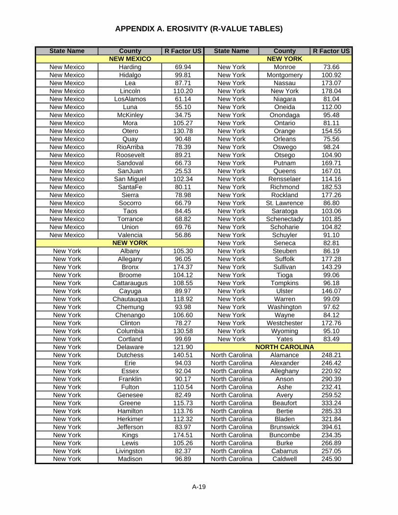
APPENDIX A. EROSIVITY (R-VALUE TABLES)
State Name County R Factor US State Name County R Factor USNEW MEXICO NEW YORK
New Mexico Harding 69.94 New York Monroe 73.66New Mexico Hidalgo 99.81 New York Montgomery 100.92New Mexico Lea 87.71 New York Nassau 173.07New Mexico Lincoln 110.20 New York New York 178.04New Mexico LosAlamos 61.14 New York Niagara 81.04New Mexico Luna 55.10 New York Oneida 112.00New Mexico McKinley 34.75 New York Onondaga 95.48New Mexico Mora 105.27 New York Ontario 81.11New Mexico Otero 130.78 New York Orange 154.55New Mexico Quay 90.48 New York Orleans 75.56New Mexico RioArriba 78.39 New York Oswego 98.24New Mexico Roosevelt 89.21 New York Otsego 104.90New Mexico Sandoval 66.73 New York Putnam 169.71New Mexico SanJuan 25.53 New York Queens 167.01New Mexico San Miguel 102.34 New York Rensselaer 114.16New Mexico SantaFe 80.11 New York Richmond 182.53New Mexico Sierra 78.98 New York Rockland 177.26New Mexico Socorro 66.79 New York St. Lawrence 86.80New Mexico Taos 84.45 New York Saratoga 103.06New Mexico Torrance 68.82 New York Schenectady 101.85New Mexico Union 69.76 New York Schoharie 104.82New Mexico Valencia 56.86 New York Schuyler 91.10
NEW YORK New York Seneca 82.81New York Albany 105.30 New York Steuben 86.19New York Allegany 96.05 New York Suffolk 177.28New York Bronx 174.37 New York Sullivan 143.29New York Broome 104.12 New York Tioga 99.06New York Cattaraugus 108.55 New York Tompkins 96.18New York Cayuga 89.97 New York Ulster 146.07New York Chautauqua 118.92 New York Warren 99.09New York Chemung 93.98 New York Washington 97.62New York Chenango 106.60 New York Wayne 84.12New York Clinton 78.27 New York Westchester 172.76New York Columbia 130.58 New York Wyoming 95.10New York Cortland 99.69 New York Yates 83.49New York Delaware 121.90 NORTH CAROLINANew York Dutchess 140.51 North Carolina Alamance 248.21New York Erie 94.03 North Carolina Alexander 246.42New York Essex 92.04 North Carolina Alleghany 220.92New York Franklin 90.17 North Carolina Anson 290.39New York Fulton 110.54 North Carolina Ashe 232.41New York Genesee 82.49 North Carolina Avery 259.52New York Greene 115.73 North Carolina Beaufort 333.24New York Hamilton 113.76 North Carolina Bertie 285.33New York Herkimer 112.32 North Carolina Bladen 321.84New York Jefferson 83.97 North Carolina Brunswick 394.61New York Kings 174.51 North Carolina Buncombe 234.35New York Lewis 105.26 North Carolina Burke 266.89New York Livingston 82.37 North Carolina Cabarrus 257.05New York Madison 96.89 North Carolina Caldwell 245.90
A-19
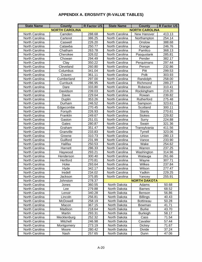
APPENDIX A. EROSIVITY (R-VALUE TABLES)
State Name County R Factor US State Name County R Factor USNORTH CAROLINA NORTH CAROLINA
North Carolina Camden 288.68 North Carolina New Hanover 413.13North Carolina Carteret 386.25 North Carolina Northampton 254.14North Carolina Caswell 226.20 North Carolina Onslow 388.68North Carolina Catawba 250.77 North Carolina Orange 246.76North Carolina Chatham 263.78 North Carolina Pamlico 368.13North Carolina Cherokee 326.02 North Carolina Pasquotank 285.81North Carolina Chowan 294.49 North Carolina Pender 382.17North Carolina Clay 350.22 North Carolina Perquimans 297.44North Carolina Cleveland 260.80 North Carolina Person 232.86North Carolina Columbus 341.04 North Carolina Pitt 299.53North Carolina Craven 361.11 North Carolina Polk 303.93North Carolina Cumberland 297.00 North Carolina Randolph 258.00North Carolina Currituck 286.95 North Carolina Richmond 289.27North Carolina Dare 333.80 North Carolina Robeson 310.41North Carolina Davidson 239.03 North Carolina Rockingham 219.20North Carolina Davie 229.64 North Carolina Rowan 239.82North Carolina Duplin 353.26 North Carolina Rutherford 275.48North Carolina Durham 246.52 North Carolina Sampson 323.61North Carolina Edgecombe 270.45 North Carolina Scotland 300.11North Carolina Forsyth 226.93 North Carolina Stanly 270.61North Carolina Franklin 249.67 North Carolina Stokes 229.82North Carolina Gaston 251.01 North Carolina Surry 224.88North Carolina Gates 280.87 North Carolina Swain 321.36North Carolina Graham 351.47 North Carolina Transylvania 411.56North Carolina Granville 233.83 North Carolina Tyrrell 323.06North Carolina Greene 310.73 North Carolina Union 280.13North Carolina Guilford 231.99 North Carolina Vance 233.90North Carolina Halifax 250.53 North Carolina Wake 254.62North Carolina Harnett 286.33 North Carolina Warren 237.25North Carolina Haywood 293.21 North Carolina Washington 314.96North Carolina Henderson 300.40 North Carolina Watauga 261.66North Carolina Hertford 270.81 North Carolina Wayne 307.71North Carolina Hoke 293.64 North Carolina Wilkes 237.84North Carolina Hyde 342.17 North Carolina Wilson 277.47North Carolina Iredell 234.02 North Carolina Yadkin 229.25North Carolina Jackson 375.85 North Carolina Yancey 255.91North Carolina Johnston 278.37 NORTH DAKOTANorth Carolina Jones 360.55 North Dakota Adams 50.68North Carolina Lee 279.88 North Dakota Barnes 68.52North Carolina Lenoir 340.28 North Dakota Benson 56.86North Carolina Lincoln 256.81 North Dakota Billings 40.43North Carolina McDowell 258.19 North Dakota Bottineau 50.28North Carolina Macon 367.15 North Dakota Bowman 41.71North Carolina Madison 218.64 North Dakota Burke 43.70North Carolina Martin 293.31 North Dakota Burleigh 58.17North Carolina Mecklenburg 252.32 North Dakota Cass 71.54North Carolina Mitchell 246.98 North Dakota Cavalier 57.44North Carolina Montgomery 273.19 North Dakota Dickey 71.67North Carolina Moore 280.42 North Dakota Divide 37.24North Carolina Nash 257.65 North Dakota Dunn 47.06
A-20

APPENDIX A. EROSIVITY (R-VALUE TABLES)
State Name County R Factor US State Name County R Factor USNORTH DAKOTA OHIO
North Dakota Eddy 62.29 Ohio Carroll 127.57North Dakota Emmons 57.82 Ohio Champaign 148.11North Dakota Foster 63.99 Ohio Clark 153.17North Dakota Golden Valley 36.34 Ohio Clermont 176.67North Dakota Grand Forks 64.30 Ohio Clinton 165.42North Dakota Grant 55.96 Ohio Columbiana 120.53North Dakota Griggs 68.61 Ohio Coshocton 135.63North Dakota Hettinger 50.24 Ohio Crawford 137.05North Dakota Kidder 60.77 Ohio Cuyahoga 119.40North Dakota La Moure 71.11 Ohio Darke 147.96North Dakota Logan 64.97 Ohio Defiance 128.35North Dakota McHenry 52.19 Ohio Delaware 143.66North Dakota McIntosh 65.37 Ohio Erie 121.37North Dakota McKenzie 39.32 Ohio Fairfield 145.56North Dakota McLean 53.28 Ohio Fayette 152.07North Dakota Mercer 52.12 Ohio Franklin 148.30North Dakota Morton 55.92 Ohio Fulton 121.45North Dakota Mountrial 46.72 Ohio Gallia 157.80North Dakota Nelson 63.59 Ohio Geauga 130.67North Dakota Oliver 55.50 Ohio Greene 155.73North Dakota Pembina 59.00 Ohio Guernsey 127.79North Dakota Pierce 53.93 Ohio Hamilton 176.52North Dakota Ramsey 57.81 Ohio Hancock 131.31North Dakota Ransom 73.45 Ohio Hardin 134.63North Dakota Renville 47.57 Ohio Harrison 129.97North Dakota Richland 78.99 Ohio Henry 126.28North Dakota Rolette 54.92 Ohio Highland 169.25North Dakota Sargent 74.21 Ohio Hocking 147.62North Dakota Sheridan 56.04 Ohio Holmes 132.79North Dakota Sioux 54.95 Ohio Huron 128.62North Dakota Slope 42.97 Ohio Jackson 154.57North Dakota Stark 49.12 Ohio Jefferson 127.81North Dakota Steele 68.32 Ohio Knox 143.17North Dakota Stutsman 64.75 Ohio Lake 116.48North Dakota Towner 55.89 Ohio Lawrence 166.01North Dakota Traill 69.03 Ohio Licking 145.11North Dakota Walsh 59.27 Ohio Logan 138.40North Dakota Ward 50.07 Ohio Lorain 117.42North Dakota Wells 58.68 Ohio Lucas 115.14North Dakota Williams 36.67 Ohio Madison 145.31
OHIO Ohio Mahoning 118.33Ohio Adams 171.14 Ohio Marion 135.84Ohio Allen 132.20 Ohio Medina 122.18Ohio Ashland 135.73 Ohio Meigs 146.16Ohio Ashtabula 123.70 Ohio Mercer 136.74Ohio Athens 141.32 Ohio Miami 145.30Ohio Auglaize 132.87 Ohio Monroe 137.83Ohio Belmont 132.06 Ohio Montgomery 152.75Ohio Brown 181.41 Ohio Morgan 143.14Ohio Butler 168.11 Ohio Morrow 142.78
A-21

APPENDIX A. EROSIVITY (R-VALUE TABLES)
State Name County R Factor US State Name County R Factor USOHIO OKLAHOMA
Ohio Muskingum 139.92 Oklahoma Delaware 285.82Ohio Noble 131.53 Oklahoma Dewey 170.09Ohio Ottawa 115.54 Oklahoma Ellis 141.11Ohio Paulding 129.04 Oklahoma Garfield 208.92Ohio Perry 145.85 Oklahoma Garvin 257.36Ohio Pickaway 151.18 Oklahoma Grady 235.40Ohio Pike 156.55 Oklahoma Grant 196.24Ohio Portage 123.73 Oklahoma Greer 168.20Ohio Preble 160.54 Oklahoma Harmon 154.22Ohio Putnam 129.62 Oklahoma Harper 145.57Ohio Richland 138.31 Oklahoma Haskell 313.90Ohio Ross 154.08 Oklahoma Hughes 283.96Ohio Sandusky 121.24 Oklahoma Jackson 171.06Ohio Scioto 156.87 Oklahoma Jefferson 231.08Ohio Seneca 128.79 Oklahoma Johnston 290.62Ohio Shelby 139.36 Oklahoma Kay 219.30Ohio Stark 123.94 Oklahoma Kingfisher 209.17Ohio Summit 123.63 Oklahoma Kiowa 188.11Ohio Trumbull 116.92 Oklahoma Latimer 343.88Ohio Tuscarawas 130.09 Oklahoma Le Flore 342.52Ohio Union 138.65 Oklahoma Lincoln 251.32Ohio Van Wert 134.73 Oklahoma Logan 223.05Ohio Vinton 152.10 Oklahoma Love 267.74Ohio Warren 165.99 Oklahoma McClain 249.96Ohio Washington 138.56 Oklahoma McCurtain 367.27Ohio Wayne 126.51 Oklahoma McIntosh 290.74Ohio Williams 125.53 Oklahoma Major 175.27Ohio Wood 121.12 Oklahoma Marshall 289.66Ohio Wyandot 132.39 Oklahoma Mayes 281.95
OKLAHOMA Oklahoma Murray 274.08Oklahoma Adair 304.06 Oklahoma Muskogee 282.70Oklahoma Alfalfa 180.02 Oklahoma Noble 227.55Oklahoma Atoka 309.52 Oklahoma Nowata 252.73Oklahoma Beaver 124.27 Oklahoma Okfuskee 270.93Oklahoma Beckham 163.60 Oklahoma Oklahoma 236.05Oklahoma Blaine 191.24 Oklahoma Okmulgee 274.40Oklahoma Bryan 309.81 Oklahoma Osage 233.26Oklahoma Caddo 203.56 Oklahoma Ottawa 274.43Oklahoma Canadian 218.26 Oklahoma Pawnee 239.80Oklahoma Carter 256.99 Oklahoma Payne 235.28Oklahoma Cherokee 296.70 Oklahoma Pittsburg 311.67Oklahoma Choctaw 331.29 Oklahoma Pontotoc 283.55Oklahoma Cimarron 79.84 Oklahoma Pottawatomie 262.40Oklahoma Cleveland 249.15 Oklahoma Pushmataha 353.19Oklahoma Coal 292.60 Oklahoma Roger Mills 155.71Oklahoma Comanche 211.07 Oklahoma Rogers 263.31Oklahoma Cotton 218.02 Oklahoma Seminole 265.57Oklahoma Craig 265.96 Oklahoma Sequoyah 299.24Oklahoma Creek 253.93 Oklahoma Stephens 237.78Oklahoma Custer 188.19 Oklahoma Texas 100.36
A-22

APPENDIX A. EROSIVITY (R-VALUE TABLES)
State Name County R Factor US State Name County R Factor USOKLAHOMA PENNSYLVANIA
Oklahoma Tillman 194.35 Pennsylvania Bedford 121.80Oklahoma Tulsa 259.69 Pennsylvania Berks 165.88Oklahoma Wagoner 278.30 Pennsylvania Blair 124.55Oklahoma Washington 243.44 Pennsylvania Bradford 100.62Oklahoma Washita 188.58 Pennsylvania Bucks 176.63Oklahoma Woods 157.01 Pennsylvania Butler 125.41Oklahoma Woodward 151.38 Pennsylvania Cambria 139.40
OREGON Pennsylvania Cameron 122.32Oregon Baker 32.50 Pennsylvania Carbon 166.20Oregon Benton 291.07 Pennsylvania Centre 125.31Oregon Clackamas 160.83 Pennsylvania Chester 175.02Oregon Clatsop 327.37 Pennsylvania Clarion 128.99Oregon Columbia 118.05 Pennsylvania Clearfield 123.46Oregon Coos 267.10 Pennsylvania Clinton 127.77Oregon Crook 22.65 Pennsylvania Columbia 138.16Oregon Curry 403.82 Pennsylvania Crawford 126.62Oregon Deschutes 114.79 Pennsylvania Cumberland 137.65Oregon Douglas 236.53 Pennsylvania Dauphin 146.23Oregon Gilliam 11.88 Pennsylvania Delaware 176.28Oregon Grant 28.16 Pennsylvania Elk 125.13Oregon Harney 30.23 Pennsylvania Erie 124.30Oregon HoodRiver 155.11 Pennsylvania Fayette 135.72Oregon Jackson 74.73 Pennsylvania Forest 122.67Oregon Jefferson 110.45 Pennsylvania Franklin 142.02Oregon Josephine 365.36 Pennsylvania Fulton 127.49Oregon Klamath 83.32 Pennsylvania Greene 130.10Oregon Lake 43.58 Pennsylvania Huntingdon 125.06Oregon Lane 267.15 Pennsylvania Indiana 136.39Oregon Lincoln 363.60 Pennsylvania Jefferson 125.37Oregon Linn 120.50 Pennsylvania Juniata 134.21Oregon Linn 121.07 Pennsylvania Lackawanna 137.02Oregon Malheur 15.29 Pennsylvania Lancaster 155.75Oregon Marion 140.88 Pennsylvania Lawrence 120.16Oregon Morrow 21.77 Pennsylvania Lebanon 157.15Oregon Multnomah 185.42 Pennsylvania Lehigh 163.18Oregon Polk 361.34 Pennsylvania Luzerne 144.18Oregon Sherman 14.14 Pennsylvania Lycoming 122.18Oregon Tillamook 405.23 Pennsylvania McKean 117.37Oregon Umatilla 31.43 Pennsylvania Mercer 125.16Oregon Union 48.54 Pennsylvania Mifflin 129.19Oregon Wallowa 44.79 Pennsylvania Monroe 162.55Oregon Wasco 97.14 Pennsylvania Montgomery 173.47Oregon Washington 219.17 Pennsylvania Montour 134.26Oregon Wheeler 22.74 Pennsylvania Northampton 165.37Oregon Yamhill 321.43 Pennsylvania Northumberland 140.06
PENNSYLVANIA Pennsylvania Perry 136.28Pennsylvania Adams 145.86 Pennsylvania Philadelphia 178.26Pennsylvania Allegheny 118.53 Pennsylvania Pike 141.33Pennsylvania Armstrong 123.47 Pennsylvania Potter 113.05Pennsylvania Beaver 118.01 Pennsylvania Schuylkill 168.51
A-23

APPENDIX A. EROSIVITY (R-VALUE TABLES)
State Name County R Factor US State Name County R Factor USPENNSYLVANIA SOUTH CAROLINA
Pennsylvania Snyder 138.62 South Carolina Lee 301.43Pennsylvania Somerset 132.25 South Carolina Lexington 316.46Pennsylvania Sullivan 127.12 South Carolina McCormick 292.44Pennsylvania Susquehanna 117.92 South Carolina Marion 334.13Pennsylvania Tioga 95.78 South Carolina Marlboro 299.34Pennsylvania Union 139.49 South Carolina Newberry 285.85Pennsylvania Venango 128.94 South Carolina Oconee 331.91Pennsylvania Warren 123.74 South Carolina Orangeburg 334.99Pennsylvania Washington 124.59 South Carolina Pickens 332.14Pennsylvania Wayne 130.22 South Carolina Richland 306.14Pennsylvania Westmoreland 128.56 South Carolina Saluda 295.71Pennsylvania Wyoming 117.29 South Carolina Spartanburg 284.33Pennsylvania York 148.92 South Carolina Sumter 318.82
RHODE ISLAND South Carolina Union 285.19Rhode Island Bristol 163.63 South Carolina Williamsburg 352.05Rhode Island Kent 173.47 South Carolina York 274.83Rhode Island Newport 166.73 SOUTH DAKOTARhode Island Providence 162.65 South Dakota Aurora 87.00Rhode Island Washington 179.01 South Dakota Beadle 78.13
SOUTH CAROLINA South Dakota Bennett 68.93South Carolina Abbeville 284.59 South Dakota Bon Homme 105.77South Carolina Aiken 318.68 South Dakota Brookings 100.68South Carolina Allendale 350.80 South Dakota Brown 73.26South Carolina Anderson 278.76 South Dakota Brule 83.45South Carolina Bamberg 342.75 South Dakota Buffalo 73.18South Carolina Barnwell 325.33 South Dakota Butte 43.84South Carolina Beaufort 411.07 South Dakota Campbell 61.34South Carolina Berkeley 385.99 South Dakota Charles Mix 96.93South Carolina Calhoun 318.89 South Dakota Clark 83.54South Carolina Charleston 399.73 South Dakota Clay 113.86South Carolina Cherokee 270.30 South Dakota Codington 89.93South Carolina Chester 282.24 South Dakota Corson 57.78South Carolina Chesterfield 296.66 South Dakota Custer 57.02South Carolina Clarendon 330.08 South Dakota Davison 90.62South Carolina Colleton 386.58 South Dakota Day 81.17South Carolina Darlington 304.44 South Dakota Deuel 98.22South Carolina Dillon 309.97 South Dakota Dewey 60.83South Carolina Dorchester 373.99 South Dakota Douglas 95.27South Carolina Edgefield 298.15 South Dakota Edmunds 68.56South Carolina Fairfield 296.21 South Dakota Fall River 48.73South Carolina Florence 318.20 South Dakota Faulk 68.48South Carolina Georgetown 396.18 South Dakota Grant 87.85South Carolina Greenville 317.09 South Dakota Gregory 97.98South Carolina Greenwood 284.06 South Dakota Haakon 59.30South Carolina Hampton 370.18 South Dakota Hamlin 95.05South Carolina Horry 359.81 South Dakota Hand 71.19South Carolina Jasper 397.23 South Dakota Hanson 93.34South Carolina Kershaw 287.03 South Dakota Harding 43.55South Carolina Lancaster 286.27 South Dakota Hughes 67.74South Carolina Laurens 282.14 South Dakota Hutchinson 100.30
A-24

APPENDIX A. EROSIVITY (R-VALUE TABLES)
State Name County R Factor US State Name County R Factor USSOUTH DAKOTA TENNESSEE
South Dakota Hyde 70.92 Tennessee Crockett 327.54South Dakota Jackson 61.93 Tennessee Cumberland 297.03South Dakota Jerauld 80.70 Tennessee Davidson 278.71South Dakota Jones 66.22 Tennessee Decatur 340.05South Dakota Kingsbury 93.20 Tennessee De Kalb 304.15South Dakota Lake 98.17 Tennessee Dickson 303.16South Dakota Lawrence 62.72 Tennessee Dyer 309.61South Dakota Lincoln 111.58 Tennessee Fayette 353.77South Dakota Lyman 72.49 Tennessee Fentress 272.77South Dakota McCook 100.07 Tennessee Franklin 333.47South Dakota McPherson 66.66 Tennessee Gibson 324.44South Dakota Marshall 77.10 Tennessee Giles 343.93South Dakota Meade 52.86 Tennessee Grainger 225.07South Dakota Mellette 70.20 Tennessee Greene 203.46South Dakota Miner 90.48 Tennessee Grundy 338.89South Dakota Minnehaha 105.51 Tennessee Hamblen 201.39South Dakota Moody 103.13 Tennessee Hamilton 303.40South Dakota Pennington 59.70 Tennessee Hancock 210.90South Dakota Perkins 52.63 Tennessee Hardeman 355.08South Dakota Potter 65.62 Tennessee Hardin 362.07South Dakota Roberts 82.66 Tennessee Hawkins 196.41South Dakota Sanborn 83.19 Tennessee Haywood 329.21South Dakota Shannon 57.78 Tennessee Henderson 334.05South Dakota Spink 76.08 Tennessee Henry 308.13South Dakota Stanley 62.98 Tennessee Hickman 319.97South Dakota Sully 66.57 Tennessee Houston 299.72South Dakota Todd 75.42 Tennessee Humphreys 318.60South Dakota Tripp 86.68 Tennessee Jackson 281.77South Dakota Turner 106.42 Tennessee Jefferson 203.66South Dakota Union 119.62 Tennessee Johnson 212.72South Dakota Walworth 63.27 Tennessee Knox 246.81South Dakota Yankton 106.65 Tennessee Lake 298.79South Dakota Ziebach 57.51 Tennessee Lauderdale 315.86
TENNESSEE Tennessee Lawrence 351.50Tennessee Anderson 271.01 Tennessee Lewis 335.29Tennessee Bedford 315.69 Tennessee Lincoln 327.62Tennessee Benton 319.99 Tennessee Loudon 272.38Tennessee Bledsoe 304.06 Tennessee McMinn 294.21Tennessee Blount 271.68 Tennessee McNairy 365.20Tennessee Bradley 301.08 Tennessee Macon 284.51Tennessee Campbell 257.65 Tennessee Madison 336.10Tennessee Cannon 316.51 Tennessee Marion 328.87Tennessee Carroll 329.35 Tennessee Marshall 333.65Tennessee Carter 215.39 Tennessee Maury 323.53Tennessee Cheatham 285.81 Tennessee Meigs 285.01Tennessee Chester 346.56 Tennessee Monroe 297.84Tennessee Claiborne 235.05 Tennessee Montgomery 275.29Tennessee Clay 271.48 Tennessee Moore 324.68Tennessee Cocke 225.64 Tennessee Morgan 282.69Tennessee Coffee 325.37 Tennessee Obion 316.60
A-25

APPENDIX A. EROSIVITY (R-VALUE TABLES)
State Name County R Factor US State Name County R Factor USTENNESSEE TEXAS
Tennessee Overton 281.68 Texas Brazos 326.09Tennessee Perry 341.86 Texas Brewster 89.33Tennessee Pickett 264.13 Texas Briscoe 129.51Tennessee Polk 315.81 Texas Brooks 246.46Tennessee Putnam 296.32 Texas Brown 200.72Tennessee Rhea 297.30 Texas Burleson 311.64Tennessee Roane 272.70 Texas Burnet 229.37Tennessee Robertson 268.70 Texas Caldwell 280.12Tennessee Rutherford 311.11 Texas Calhoun 380.63Tennessee Scott 265.47 Texas Callahan 183.40Tennessee Sequatchie 323.16 Texas Cameron 270.67Tennessee Sevier 261.01 Texas Camp 342.89Tennessee Shelby 345.53 Texas Carson 123.81Tennessee Smith 281.86 Texas Cass 361.37Tennessee Stewart 286.63 Texas Castro 100.51Tennessee Sullivan 183.74 Texas Chambers 498.24Tennessee Sumner 276.10 Texas Cherokee 355.39Tennessee Tipton 326.46 Texas Childress 138.76Tennessee Trousdale 283.40 Texas Clay 218.98Tennessee Unicoi 231.02 Texas Cochran 99.77Tennessee Union 243.22 Texas Coke 153.27Tennessee Van Buren 308.94 Texas Coleman 191.85Tennessee Warren 307.04 Texas Collin 297.26Tennessee Washington 199.69 Texas Collingsworth 140.30Tennessee Wayne 366.44 Texas Colorado 353.06Tennessee Weakley 312.77 Texas Comal 267.22Tennessee White 298.67 Texas Comanche 212.41Tennessee Williamson 303.01 Texas Concho 176.38Tennessee Wilson 294.26 Texas Cooke 267.43
TEXAS Texas Coryell 242.95Texas Anderson 335.10 Texas Cottle 142.10Texas Andrews 88.75 Texas Crane 77.89Texas Angelina 388.00 Texas Crockett 126.48Texas Aransas 346.87 Texas Crosby 129.39Texas Archer 198.99 Texas Culberson 64.44Texas Armstrong 127.97 Texas Dallam 80.29Texas Atascosa 227.91 Texas Dallas 272.76Texas Austin 352.96 Texas Dawson 112.90Texas Bailey 94.37 Texas Deaf Smith 95.14Texas Bandera 224.32 Texas Delta 332.01Texas Bastrop 289.31 Texas Denton 275.78Texas Baylor 184.28 Texas De Witt 303.08Texas Bee 299.18 Texas Dickens 138.30Texas Bell 263.11 Texas Dimmit 180.61Texas Bexar 245.42 Texas Donley 135.52Texas Blanco 244.31 Texas Duval 232.03Texas Borden 126.79 Texas Eastland 200.52Texas Bosque 247.96 Texas Ector 79.12Texas Bowie 365.61 Texas Edwards 186.68Texas Brazoria 478.11 Texas Ellis 273.05
A-26

APPENDIX A. EROSIVITY (R-VALUE TABLES)
State Name County R Factor US State Name County R Factor USTEXAS TEXAS
Texas El Paso 39.01 Texas Jasper 495.30Texas Erath 224.34 Texas Jeff Davis 86.81Texas Falls 276.20 Texas Jefferson 541.24Texas Fannin 323.35 Texas Jim Hogg 219.69Texas Fayette 319.75 Texas Jim Wells 263.93Texas Fisher 158.98 Texas Johnson 250.76Texas Floyd 126.95 Texas Jones 170.45Texas Foard 158.62 Texas Karnes 258.09Texas Fort Bend 401.81 Texas Kaufman 295.60Texas Franklin 338.41 Texas Kendall 258.51Texas Freestone 314.84 Texas Kenedy 261.02Texas Frio 209.27 Texas Kent 139.41Texas Gaines 97.99 Texas Kerr 218.13Texas Galveston 463.53 Texas Kimble 188.68Texas Garza 129.45 Texas King 150.46Texas Gillespie 227.57 Texas Kinney 173.96Texas Glasscock 115.78 Texas Kleberg 273.62Texas Goliad 312.40 Texas Knox 168.80Texas Gonzales 296.39 Texas Lamar 339.18Texas Gray 134.88 Texas Lamb 104.18Texas Grayson 296.43 Texas Lampasas 223.77Texas Gregg 365.74 Texas La Salle 196.35Texas Grimes 359.62 Texas Lavaca 334.29Texas Guadalupe 275.71 Texas Lee 296.49Texas Hale 114.42 Texas Leon 324.24Texas Hall 129.95 Texas Liberty 479.33Texas Hamilton 222.37 Texas Limestone 294.05Texas Hansford 105.23 Texas Lipscomb 129.91Texas Hardeman 161.46 Texas Live Oak 250.26Texas Hardin 511.52 Texas Llano 212.70Texas Harris 435.78 Texas Loving 57.51Texas Harrison 375.43 Texas Lubbock 115.88Texas Hartley 87.21 Texas Lynn 118.39Texas Haskell 174.40 Texas McCulloch 188.44Texas Hays 266.09 Texas McLennan 259.20Texas Hemphill 134.14 Texas McMullen 215.41Texas Henderson 313.31 Texas Madison 344.50Texas Hidalgo 240.42 Texas Marion 364.09Texas Hill 264.80 Texas Martin 105.31Texas Hockley 108.70 Texas Mason 202.09Texas Hood 229.97 Texas Matagorda 425.47Texas Hopkins 344.01 Texas Maverick 178.17Texas Houston 350.89 Texas Medina 218.96Texas Howard 123.53 Texas Menard 180.25Texas Hudspeth 51.61 Texas Midland 92.58Texas Hunt 316.01 Texas Milam 279.91Texas Hutchinson 114.01 Texas Mills 201.56Texas Irion 138.40 Texas Mitchell 138.63Texas Jack 224.06 Texas Montague 241.29Texas Jackson 383.17 Texas Montgomery 408.72
A-27

APPENDIX A. EROSIVITY (R-VALUE TABLES)
State Name County R Factor US State Name County R Factor USTEXAS TEXAS
Texas Moore 99.71 Texas Taylor 175.50Texas Morris 353.68 Texas Terrell 96.42Texas Motley 132.89 Texas Terry 106.85Texas Nacogdoches 387.37 Texas Throckmorton 189.60Texas Navarro 288.63 Texas Titus 355.62Texas Newton 513.71 Texas Tom Green 150.71Texas Nolan 162.89 Texas Travis 257.26Texas Nueces 291.16 Texas Trinity 374.95Texas Ochiltree 116.75 Texas Tyler 467.31Texas Oldham 92.03 Texas Upshur 346.36Texas Orange 559.83 Texas Upton 93.12Texas Palo Pinto 221.81 Texas Uvalde 197.83Texas Panola 392.80 Texas Val Verde 142.70Texas Parker 234.33 Texas Van Zandt 316.71Texas Parmer 91.03 Texas Victoria 348.25Texas Pecos 87.25 Texas Walker 380.49Texas Polk 422.57 Texas Waller 367.80Texas Potter 110.75 Texas Ward 64.78Texas Presidio 81.26 Texas Washington 339.04Texas Rains 323.27 Texas Webb 198.22Texas Randall 112.16 Texas Wharton 388.36Texas Reagan 119.74 Texas Wheeler 142.10Texas Real 209.80 Texas Wichita 196.57Texas Red River 348.12 Texas Wilbarger 177.49Texas Reeves 62.64 Texas Willacy 270.86Texas Refugio 351.63 Texas Williamson 261.80Texas Roberts 123.36 Texas Wilson 245.82Texas Robertson 293.73 Texas Winkler 70.26Texas Rockwall 298.82 Texas Wise 249.55Texas Runnels 174.98 Texas Wood 323.99Texas Rusk 368.45 Texas Yoakum 98.58Texas Sabine 458.16 Texas Young 209.68Texas San Augustine 431.00 Texas Zapata 200.82Texas San Jacinto 425.26 Texas Zavala 177.40Texas San Patricio 318.52 UTAHTexas San Saba 200.94 Utah Beaver 42.55Texas Schleicher 157.30 Utah BoxElder 46.28Texas Scurry 144.22 Utah Cache 32.87Texas Shackelford 187.83 Utah Carbon 18.23Texas Shelby 416.50 Utah Daggett 24.75Texas Sherman 94.34 Utah Davis 37.24Texas Smith 336.82 Utah Duchesne 28.45Texas Somervell 235.79 Utah Emery 25.38Texas Starr 221.89 Utah Garfield 32.79Texas Stephens 200.13 Utah Grand 26.75Texas Sterling 131.84 Utah Iron 37.64Texas Stonewall 151.69 Utah Juab 27.78Texas Sutton 163.39 Utah Kane 36.49Texas Swisher 116.82 Utah Millard 26.66Texas Tarrant 252.95 Utah Morgan 40.93
A-28

APPENDIX A. EROSIVITY (R-VALUE TABLES)
State Name County R Factor US State Name County R Factor USUTAH VIRGINIA
Utah Piute 42.55 Virginia Chesterfield 208.96Utah Rich 26.75 Virginia Clarke 145.41Utah SaltLake 50.29 Virginia Craig 156.54Utah SanJuan 34.09 Virginia Culpeper 179.01Utah Sanpete 30.36 Virginia Cumberland 185.48Utah Sevier 34.96 Virginia Dickenson 186.19Utah Summit 37.56 Virginia Dinwiddie 219.80Utah Tooele 45.99 Virginia Essex 204.28Utah Uintah 28.02 Virginia Fairfax 168.12Utah Utah 42.11 Virginia Fauquier 164.51Utah Wasatch 37.37 Virginia Floyd 195.63Utah Washington 40.70 Virginia Fluvanna 180.24Utah Wayne 26.79 Virginia Franklin 203.31Utah Weber 46.28 Virginia Frederick 135.55
VERMONT Virginia Giles 150.31Vermont Addison 93.46 Virginia Gloucester 220.34Vermont Bennington 131.23 Virginia Goochland 195.01Vermont Caledonia 98.81 Virginia Grayson 190.46Vermont Chittenden 90.99 Virginia Greene 186.90Vermont Essex 100.77 Virginia Greensville 235.45Vermont Franklin 95.97 Virginia Halifax 209.27Vermont Grand Isle 72.13 Virginia Hanover 197.19Vermont Lamoille 105.65 Virginia Henrico 206.66Vermont Orange 91.71 Virginia Henry 221.25Vermont Orleans 97.62 Virginia Highland 138.78Vermont Rutland 108.38 Virginia Isle of Wight 258.17Vermont Washington 99.42 Virginia James City 231.64Vermont Windham 126.56 Virginia King and Queen 212.59Vermont Windsor 103.12 Virginia King George 185.08
VIRGINIA Virginia King William 210.25Virginia Accomack 205.76 Virginia Lancaster 208.33Virginia Albemarle 189.88 Virginia Lee 224.99Virginia Alleghany 145.02 Virginia Loudoun 157.35Virginia Amelia 202.67 Virginia Louisa 191.89Virginia Amherst 178.84 Virginia Lunenburg 215.60Virginia Appomattox 189.90 Virginia Madison 178.60Virginia Arlington 177.60 Virginia Mathews 226.68Virginia Augusta 151.24 Virginia Mecklenburg 219.46Virginia Bath 151.25 Virginia Middlesex 215.65Virginia Bedford 177.86 Virginia Montgomery 158.62Virginia Bland 148.06 Virginia Nelson 190.35Virginia Botetourt 160.76 Virginia New Kent 214.39Virginia Brunswick 224.15 Virginia Northampton 209.81Virginia Buchanan 174.53 Virginia Northumberland 202.31Virginia Buckingham 185.34 Virginia Nottoway 208.94Virginia Campbell 193.77 Virginia Orange 187.86Virginia Caroline 189.79 Virginia Page 151.42Virginia Carroll 194.45 Virginia Patrick 229.82Virginia Charles City 220.14 Virginia Pittsylvania 203.01Virginia Charlotte 202.68 Virginia Powhatan 193.85
A-29

APPENDIX A. EROSIVITY (R-VALUE TABLES)
State Name County R Factor US State Name County R Factor USVIRGINIA WASHINGTON
Virginia Prince Edward 204.82 Washington Mason 382.51Virginia Prince George 226.45 Washington Okanogan 85.82Virginia Prince William 166.61 Washington Pacific 257.76Virginia Pulaski 145.28 Washington Pacific 170.72Virginia Rappahannock 170.69 Washington PendOreille 39.69Virginia Richmond 206.85 Washington Pierce 244.01Virginia Roanoke 161.81 Washington Skagit 184.67Virginia Rockbridge 160.38 Washington Skamania 191.51Virginia Rockingham 135.19 Washington Snohomish 232.10Virginia Russell 185.25 Washington Spokane 24.25Virginia Scott 197.80 Washington Stevens 39.56Virginia Shenandoah 131.14 Washington Thurston 150.81Virginia Smyth 179.73 Washington Wahkiakum 209.41Virginia Southampton 252.83 Washington Wahkiakum 151.79Virginia Spotsylvania 184.50 Washington WallaWalla 27.75Virginia Stafford 175.55 Washington Whatcom 156.02Virginia Surry 236.73 Washington Whitman 19.39Virginia Sussex 237.17 Washington Yakima 121.15Virginia Tazewell 166.07 WEST VIRGINIAVirginia Warren 151.86 West Virginia Barbour 150.34Virginia Washington 184.37 West Virginia Berkeley 134.54Virginia Westmoreland 195.57 West Virginia Boone 167.61Virginia Wise 195.48 West Virginia Braxton 157.15Virginia Wythe 140.08 West Virginia Brooke 126.77Virginia York 243.55 West Virginia Cabell 158.31
WASHINGTON West Virginia Calhoun 148.53Washington Adams 9.08 West Virginia Clay 160.47Washington Asiton 25.47 West Virginia Doddridge 143.69Washington Benton 8.60 West Virginia Fayette 162.60Washington Chelan 212.16 West Virginia Gilmer 149.65Washington Clallam 409.46 West Virginia Grant 124.74Washington Clallam 177.33 West Virginia Greenbrier 162.46Washington Clark 191.25 West Virginia Hampshire 121.57Washington Columbia 38.55 West Virginia Hancock 121.87Washington Cowlitz 211.27 West Virginia Hardy 125.02Washington Douglas 21.36 West Virginia Harrison 137.89Washington Ferry 24.36 West Virginia Jackson 146.08Washington Franklin 7.26 West Virginia Jefferson 137.22Washington Garfield 32.70 West Virginia Kanawha 157.83Washington Grant 9.22 West Virginia Lewis 150.91Washington GraysHarbor 414.51 West Virginia Lincoln 166.87Washington Island 47.12 West Virginia Logan 174.65Washington Jefferson 495.03 West Virginia McDowell 159.93Washington Jefferson 157.52 West Virginia Marion 138.35Washington King 237.15 West Virginia Marshall 134.22Washington Kitsap 97.63 West Virginia Mason 150.73Washington Kittitas 199.35 West Virginia Mercer 139.80Washington Klickitat 74.38 West Virginia Mineral 115.69Washington Lewis 208.04 West Virginia Mingo 177.88Washington Lincoln 10.67 West Virginia Monongalia 136.09
A-30

APPENDIX A. EROSIVITY (R-VALUE TABLES)
State Name County R Factor US State Name County R Factor USWEST VIRGINIA WISCONSIN
West Virginia Monroe 139.72 Wisconsin Iron 101.54West Virginia Morgan 123.07 Wisconsin Jackson 140.00West Virginia Nicholas 171.17 Wisconsin Jefferson 133.42West Virginia Ohio 126.77 Wisconsin Juneau 134.71West Virginia Pendleton 125.13 Wisconsin Kenosha 142.89West Virginia Pleasants 140.60 Wisconsin Kewaunee 97.73West Virginia Pocahontas 165.35 Wisconsin La Crosse 143.23West Virginia Preston 156.70 Wisconsin Lafayette 154.26West Virginia Putnam 152.96 Wisconsin Langlade 108.23West Virginia Raleigh 153.32 Wisconsin Lincoln 111.42West Virginia Randolph 170.41 Wisconsin Manitowoc 105.54West Virginia Ritchie 141.78 Wisconsin Marathon 122.51West Virginia Roane 150.99 Wisconsin Marinette 94.10West Virginia Summers 138.97 Wisconsin Marquette 124.69West Virginia Taylor 137.83 Wisconsin Menominee 105.86West Virginia Tucker 161.11 Wisconsin Milwaukee 123.97West Virginia Tyler 143.03 Wisconsin Monroe 140.99West Virginia Upshur 158.77 Wisconsin Oconto 100.80West Virginia Wayne 170.35 Wisconsin Oneida 106.05West Virginia Webster 178.98 Wisconsin Outagamie 108.40West Virginia Wetzel 144.56 Wisconsin Ozaukee 119.27West Virginia Wirt 145.88 Wisconsin Pepin 134.41West Virginia Wood 138.77 Wisconsin Pierce 133.63West Virginia Wyoming 164.89 Wisconsin Polk 125.39
WISCONSIN Wisconsin Portage 122.90Wisconsin Adams 129.91 Wisconsin Price 113.87Wisconsin Ashland 103.75 Wisconsin Racine 139.91Wisconsin Barron 128.37 Wisconsin Richland 140.06Wisconsin Bayfield 103.36 Wisconsin Rock 145.01Wisconsin Brown 102.54 Wisconsin Rusk 124.97Wisconsin Buffalo 141.45 Wisconsin St. Croix 128.77Wisconsin Burnett 117.05 Wisconsin Sauk 134.85Wisconsin Calumet 110.93 Wisconsin Sawyer 118.25Wisconsin Chippewa 129.00 Wisconsin Shawano 110.21Wisconsin Clark 133.01 Wisconsin Sheboygan 122.09Wisconsin Columbia 130.01 Wisconsin Taylor 122.83Wisconsin Crawford 142.85 Wisconsin Trempealeau 139.48Wisconsin Dane 134.57 Wisconsin Vernon 141.60Wisconsin Dodge 125.21 Wisconsin Vilas 99.88Wisconsin Door 93.91 Wisconsin Walworth 145.43Wisconsin Douglas 108.51 Wisconsin Washburn 117.62Wisconsin Dunn 130.11 Wisconsin Washington 124.80Wisconsin Eau Claire 133.51 Wisconsin Waukesha 128.43Wisconsin Florence 91.13 Wisconsin Waupaca 117.16Wisconsin Fond Du Lac 116.61 Wisconsin Waushara 120.08Wisconsin Forest 100.33 Wisconsin Winnebago 113.77Wisconsin Grant 150.88 Wisconsin Wood 129.88Wisconsin Green 148.94 WYOMINGWisconsin Green Lake 120.80 Wyoming BigHorn 37.76Wisconsin Iowa 143.96 Wyoming Campbell 32.70
A-31

APPENDIX A. EROSIVITY (R-VALUE TABLES)
State Name County R Factor USWYOMING
Wyoming Carbon 38.18Wyoming Converse 30.29Wyoming Crook 63.55Wyoming Fremont 21.72Wyoming Goshen 40.31Wyoming HotSprings 21.03Wyoming Johnson 39.83Wyoming Laramie 32.40Wyoming Lincoln 27.50Wyoming Natrona 39.98Wyoming Niobrara 37.43Wyoming Park 35.13Wyoming Platte 38.18Wyoming Sheridan 28.70Wyoming Sublette 28.62Wyoming Sweetwater 14.83Wyoming Teton 33.84Wyoming Uinta 20.48Wyoming Washakie 31.08Wyoming Weston 69.62
A-32

B-1
APPENDIX B. RAPPS DECISION TREES

R Factor ≤ 145
Silt/Loam SoilsIf R < 65, use Operational RAPPS
Clay SoilsIf R < 85, use Operational RAPPS
Sand/Gravel SoilsIf R < 145, use Operational RAPPS
- (WFM 0.91)
- (ECM 0.85)
- (VB 0.80)
- (BP 0.73)
- (CS 0.73)
- (RB 0.73)
-(SB 0.72)
- (SF0.67)
- (SBB 0.59) (SBB/SF 0.73)
- (IS 0.47) (IS/SBB 0.87)
- (WFM 0.90)
- (ECM 0.83)
- (VB 0.75)
- (RB 0.73)
- (SB 0.73)
- (BP 0.73)
- (CS 0.73)
- (SF 0.72)
- (SBB 0.69) (SBB/SF 0.78)
- (IS 0.39) (IS/SBB 0.82)
- (VB 0.99)
- (SB 0.98)
- (BP 0.95)
- (CS 0.95)
- (RB 0.95)
- (WFM 0.93)
- (ECM 0.86)
- (SF 0.82)
- (SBB 0.65) (SBB/SF 0.95)
- (IS 0.52) (IS/SBB 0.88)
SLOPE < 2%
Modified Management Goal = 0.60
IndexVB – Vegetative Buffer SBB – Straw Bale BarrierSB – Sediment Basin WFM – Wood Fiber MulchIS – Interceptor Swale ECM – Erosion Control MatRB – Rock Berm BP – Brush pileCS – Compost Sock SF – Silt Fence
Decision Tree-1

145 ≤ R Factor ≤ 300
- (WFM 0.90)
- (ECM 0.81)
- (VB 0.77)
- (SB 0.69)
- (RB 0.69)
- (BP 0.69) (2BP 0.76)
- (CS 0.69) (2CS 0.76)
- (SF 0.63) (2SF 0.71)
- (SBB 0.61) (SBB/SF 0.69)
- (IS 0.46) (IS/SBB 0.87)
- (WFM 0.88)
- (ECM 0.80)
- (VB 0.71)
- (SB 0.68)
- (RB 0.68)
- (SF 0.68) (2SF 0.81)
- (BP 0.68) (2BP 0.73)
- (CS 0.68) (2CS 0.73)
- (SBB 0.68) (SBB/SF 0.68)
- (IS 0.38) (IS/SBB 0.85)
- (SB 0.98)
- (VB 0.98)
- (BP 0.96)
- (CS 0.96)
- (RB 0.96)
- (WFM 0.90)
- (SF 0.84)
- (ECM 0.82)
- (SBB 0.69) (SBB/SF 0.96)
- (IS 0.53) (IS/SBB 0.91)
SLOPE < 2%SLOPE < 2%
Sand/Gravel SoilsIf R < 185, use Operational RAPPS
Clay Soils*Silt/Loam Soils*
*Modified Management Goal = 0.60
IndexVB – Vegetative Buffer SBB – Straw Bale BarrierSB – Sediment Basin WFM – Wood Fiber MulchIS – Interceptor Swale ECM – Erosion Control MatRB – Rock Berm BP – Brush pileCS – Compost Sock SF – Silt Fence
Decision Tree-2
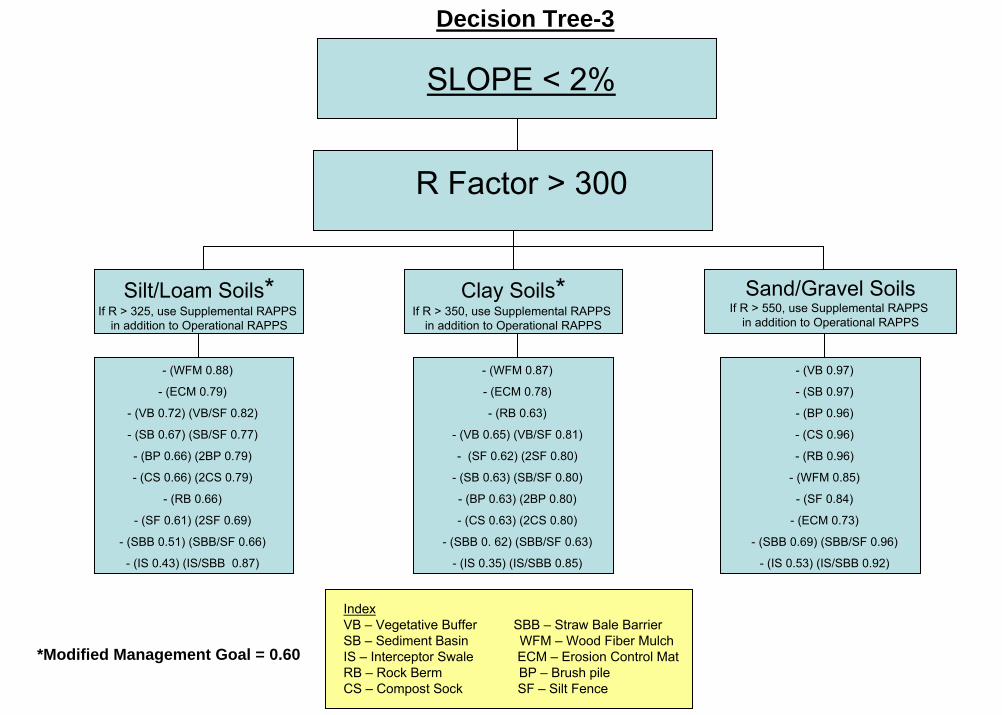
R Factor > 300
- (WFM 0.88)
- (ECM 0.79)
- (VB 0.72) (VB/SF 0.82)
- (SB 0.67) (SB/SF 0.77)
- (BP 0.66) (2BP 0.79)
- (CS 0.66) (2CS 0.79)
- (RB 0.66)
- (SF 0.61) (2SF 0.69)
- (SBB 0.51) (SBB/SF 0.66)
- (IS 0.43) (IS/SBB 0.87)
- (WFM 0.87)
- (ECM 0.78)
- (RB 0.63)
- (VB 0.65) (VB/SF 0.81)
- (SF 0.62) (2SF 0.80)
- (SB 0.63) (SB/SF 0.80)
- (BP 0.63) (2BP 0.80)
- (CS 0.63) (2CS 0.80)
- (SBB 0. 62) (SBB/SF 0.63)
- (IS 0.35) (IS/SBB 0.85)
- (VB 0.97)
- (SB 0.97)
- (BP 0.96)
- (CS 0.96)
- (RB 0.96)
- (WFM 0.85)
- (SF 0.84)
- (ECM 0.73)
- (SBB 0.69) (SBB/SF 0.96)
- (IS 0.53) (IS/SBB 0.92)
SLOPE < 2%
Sand/Gravel SoilsIf R > 550, use Supplemental RAPPS
in addition to Operational RAPPS
Clay Soils*If R > 350, use Supplemental RAPPS
in addition to Operational RAPPS
Silt/Loam Soils*If R > 325, use Supplemental RAPPS
in addition to Operational RAPPS
*Modified Management Goal = 0.60
IndexVB – Vegetative Buffer SBB – Straw Bale BarrierSB – Sediment Basin WFM – Wood Fiber MulchIS – Interceptor Swale ECM – Erosion Control MatRB – Rock Berm BP – Brush pileCS – Compost Sock SF – Silt Fence
Decision Tree-3

R Factor ≤ 45
Silt/Loam Soils Clay Soils Sand/Gravel SoilsIf R < 45, use Operational RAPPS
- (WFM 0.94)
- (ECM 0.93)
- (VB 0.90)
- (SB 0.80)
- (BP 0.70)
- (CS 0.70)
- (RB 0.70)
- (SF 0.59) (2SF 0.70)
- (IS 0.58) (IS/SBB 0.92)
- (SBB 0.51) (SBB/SF 0.71)
- (WFM 0.93)
- (ECM 0.92)
- (VB 0.87)
- (RB 0.86)
- (SB 0.86)
- (BP 0.86)
- (CS 0.86)
- (SF 0.77)
- (SBB 0.56) (SBB/SF 0.86)
- (IS 0.50) (IS/SBB 0.91)
- (VB 0.99)
- (SB 0.99)
- (WFM 0.95)
- (ECM 0.94)
- (RB 0.92)
- (BP 0.92)
- (CS 0.92)
- (SF 0.71)
- (IS 0.59) (IS/SBB 0.92)
- SBB (0.43) (SBB/SF 0.92)
SLOPE (2% - 4%)
Default Management Goal = 0.70
If R < 25, use Operational RAPPSIf R < 20, use Operational RAPPS
IndexVB – Vegetative Buffer SBB – Straw Bale BarrierSB – Sediment Basin WFM – Wood Fiber MulchIS – Interceptor Swale ECM – Erosion Control MatRB – Rock Berm BP – Brush pileCS – Compost Sock SF – Silt Fence
Decision Tree-4
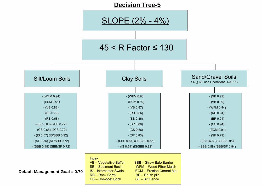
45 < R Factor ≤ 130
Silt/Loam Soils Clay Soils
- (WFM 0.94)
- (ECM 0.91)
- (VB 0.88)
- (SB 0.79)
- (RB 0.68)
- (BP 0.68) (2BP 0.72)
- (CS 0.68) (2CS 0.72)
- (IS 0.57) (IS/SBB 0.92)
- (SF 0.56) (SF/SBB 0.72)
- (SBB 0.49) (SBB/SF 0.72)
- (WFM 0.93)
- (ECM 0.89)
- (VB 0.87)
- (RB 0.86)
- (SB 0.86)
- (BP 0.86)
- (CS 0.86)
- (SF 0.83)
- (SBB 0.67) (SBB/SF 0.86)
- (IS 0.51) (IS/SBB 0.92)
- (SB 0.99)
- (VB 0.99)
- (WFM 0.94)
- (RB 0.94)
- (BP 0.94)
- (CS 0.94)
- (ECM 0.91)
- (SF 0.79)
- (IS 0.60) (IS/SBB 0.95)
- (SBB 0.58) (SBB/SF 0.94)
SLOPE (2% - 4%)
Sand/Gravel SoilsIf R < 60, use Operational RAPPS
Default Management Goal = 0.70
IndexVB – Vegetative Buffer SBB – Straw Bale BarrierSB – Sediment Basin WFM – Wood Fiber MulchIS – Interceptor Swale ECM – Erosion Control MatRB – Rock Berm BP – Brush pileCS – Compost Sock SF – Silt Fence
Decision Tree-5

R Factor > 130
Silt/Loam SoilsIf R > 175, use Supplemental RAPPS
in addition to Operational RAPPS
Clay SoilsIf R > 400, use Supplemental RAPPS
in addition to Operational RAPPS
- (WFM 0.92)
- (ECM 0.87)
- (VB 0.84)
- (SB 0.79)
- (RB 0.62)
- (BP 0.62) (2BP 0.70)
- (CS 0.62) (2CS 0.70)
- IS (0.58) (IS/SBB 0.91)
- (SF 0.52) (SF/SBB 0.62)
- (SBB 0.46) (SBB/SF 0.62)
- (WFM 0.87)
- (VB 0.81)
- (SB 0.80)
- (RB 0.79)
- (BP 0.79)
- (CS 0.79)
- (SF 0.79)
- (ECM 0.76)
- (SBB 0.69) (SBB/SF 0.91)
- (IS 0.49) (IS/SBB 0.79)
- (VB 0.99)
- (SB 0.99)
- (BP 0.96)
- (CS 0.96)
- (RB 0.96)
- (WFM 0.87)
- (SF 0.84)
- (ECM 0.77)
- (SBB 0.69) (SBB/SF 0.96)
- (IS 0.62) (IS/SBB 0.97)
SLOPE (2% - 4%)
Sand/Gravel SoilsIf R > 500, use Supplemental RAPPS
in addition to Operational RAPPS
Default Management Goal = 0.70
IndexVB – Vegetative Buffer SBB – Straw Bale BarrierSB – Sediment Basin WFM – Wood Fiber MulchIS – Interceptor Swale ECM – Erosion Control MatRB – Rock Berm BP – Brush pileCS – Compost Sock SF – Silt Fence
Decision Tree-6

R Factor ≤ 30
Silt/Loam SoilsIf Slope > 25%, use Supplemental RAPPS
in addition to Operational RAPPS
Clay SoilsIf Slope >30% , use Supplemental RAPPS
in addition to Operational RAPPS
- (WFM 0.95)
- (ECM 0.94)
- (VB 0.90)
- (SB 0.81)
- (RB 0.64)
- (BP 0.64) (2BP 0.71)
- (CS 0.64) (2CS 0.71)
- (IS 0.61) (IS/SBB 0.93)
- (SF 0.51)
- (SBB 0.38)
- (WFM 0.94)
- (ECM 0.93)
- (VB 0.87)
- (SB 0.86)
- (RB 0.84)
- (BP 0.84)
- (CS 0.84)
- (IS 0.53) (IS/SBB 0.91)
- (SF 0. 51)
- (SBB 0.19) (SBB/SF 0.84)
- (SB 0.99)
- (VB 0.98)
- (WFM 0.95)
- (ECM 0.94)
- (RB 0.82)
- (BP 0.82)
- (CS 0.82)
- (IS 0.62) (IS/SBB 0.91)
- SF (0.38) (SF/SBB 0.82)
- (SBB 0.10) (SBB/SF 0.82)
SLOPE > 4%
Sand/Gravel SoilsIf R < 30, use Operational RAPPS
Default Management Goal = 0.70
IndexVB – Vegetative Buffer SBB – Straw Bale BarrierSB – Sediment Basin WFM – Wood Fiber MulchIS – Interceptor Swale ECM – Erosion Control MatRB – Rock Berm BP – Brush pileCS – Compost Sock SF – Silt Fence
Decision Tree-7

30 < R Factor ≤ 90
Silt/Loam SoilsIf Slope > 10%, use Supplemental RAPPS
in addition to Operational RAPPS
Clay SoilsIf Slope >12% , use Supplemental RAPPS
in addition to Operational RAPPS
- (WFM 0.95)
- (ECM 0.93)
- (VB 0.89)
- (SB 0.80)
- (RB 0.63)
- (BP 0.63) (2BP 0.69)
- (CS 0.63) (2CS 0.69)
- (IS 0.61) (IS/SBB 0.93)
-(SF 0.54)
-(SBB 0.67) (SBB/SF 0.71)
- (WFM 0.93)
- (ECM 0.92)
- (VB 0.87)
- (RB 0.86)
- (SB 0.86)
- (BP 0.86)
- (CS 0.86)
- (SF 0.80)
- (SBB 0.63) (SBB/SF 0.86)
- (IS 0.53) (IS/SBB 0.93)
- (VB 0.99)
- (SB 0.99)
- (WFM 0.95)
- (ECM 0.94)
- (RB 0.93)
- (BP 0.93)
- (CS 0.93)
- (SF 0.73)
- (IS 0.62) (IS/SBB 0.94)
- (SBB 0.46) (SBB/SF 0.93)
SLOPE > 4%
Sand/Gravel SoilsIf R < 40, use Operational RAPPS
Default Management Goal = 0.70
IndexVB – Vegetative Buffer SBB – Straw Bale BarrierSB – Sediment Basin WFM – Wood Fiber MulchIS – Interceptor Swale ECM – Erosion Control MatRB – Rock Berm BP – Brush pileCS – Compost Sock SF – Silt Fence
Decision Tree-8

R Factor > 90
Silt/Loam SoilsIf R > 120 OR If R > 90 AND Slope >7%, use Supplemental RAPPS in addition to
Operational RAPPS
Clay SoilsIf R > 300, OR If R > 100 AND Slope >10%,
use Supplemental RAPPS in addition to Operational RAPPS
- (WFM 0.94)
- (ECM 0.90)
- (VB 0.87)
- (SB 0.80)
-(IS 0.61) (IS/SBB 0.93)
- (RB 0.60)
- (BP 0.60)
- (CS 0.60)
- (SF 0.52) (SF/SBB 0.71)
- (SBB 0.46) (SBB/SF 0.71)
- (WFM 0.89)
- (VB 0.86)
- (RB 0.85)
- (SB 0.85)
- (BP 0.85)
- (CS 0.85)
- (SF 0.84)
- (ECM 0.81)
- (SBB/SF 0.93)
- (IS 0.54) (IS/SBB 0.85)
- (VB 0.99)
- (SB 0.99)
- (RB 0.96)
- (BP 0.96)
- (CS 0.96)
- (WFM 0.9)
- (SF 0.84)
- (ECM 0.83)
- (SBB/SF 0.96)
- (IS 0.64) (IS/SBB 0.98)
SLOPE > 4%
Sand/Gravel SoilsIf R > 375, OR if R > 200 AND Slope >10%,
use Supplemental RAPPS in addition toOperational RAPPS
Default Management Goal = 0.70
IndexVB – Vegetative Buffer SBB – Straw Bale BarrierSB – Sediment Basin WFM – Wood Fiber MulchIS – Interceptor Swale ECM – Erosion Control MatRB – Rock Berm BP – Brush pileCS – Compost Sock SF – Silt Fence
Decision Tree-9

C-1
APPENDIX C. EXAMPLES OF RAPPS

1) Vegetative Buffer (VB) Description: A vegetative buffer is a zone of established vegetation that is conserved or promoted to guard the quality of stormwater runoff. The barrier reduces the velocity of the stormwater allowing water to infiltrate the subsurface and deposit sediment from stormwater runoff. The most effective vegetative cover consists of a low-growing, herbaceous species with a high percentage of ground coverage. Due to the “umbrella effect”, shrubs and trees can provide some means of preventing erosion by shielding the underlying soil from the impact of raindrops. However, their filtering ability is much lower than that of native grasses. Therefore, vegetation should be preserved or disturbed areas should be re-vegetated. Installation: It is recommended that at least a 20-foot wide vegetative buffer strip in a down-gradient position from the disturbed area be used prior to and during the disturbance phase of the excavation/construction. If sodding or seeding is required, adequate lead time prior to beginning soil disturbance should be planned to establish a healthy stand of grass. This may require the installation of an irrigation system. Existing vegetation should be used wherever possible. Limitations:
• Adequate land must be available for a vegetated buffer to prevent the loss of sediment from the site;
• Adequate vegetative cover must be maintained in the buffer to keep it effective; • Vegetated buffers work well with sheet flow, but they are not appropriate for controlling
concentrated flows of stormwater; • When used in areas that may have concentrated flows, additional RAPPS should be used
to disperse the flow and reduce velocity prior to the buffer; • Re-establishing vegetation on compacted soils is difficult without the use of geotextiles; • In order to remain effective, buffer widths must increase as slope steepness increases.
Maintenance Considerations: Routine maintenance is necessary to keep the vegetation in good condition. Maintenance may include: mowing, fertilizing, and irrigating. During the establishment phase, inspection and maintenance are most important. Once established, vegetated buffers do not require maintenance beyond routine procedures and periodic inspections. Vegetative buffers should be inspected after heavy rainfall and at least once a year. Operators should focus on headward erosion, gully erosion, the density of the vegetation, evidence of concentrated flows through the areas, and any damage from foot or vehicular traffic. If more than 6 inches of sediment has accumulated on the upgraded edge of the vegetative buffer, the sediment should be removed.
A 20-foot wide vegetated buffer strip between a creek and disturbed bare land. Source: Carleton College Seven-Mile Creek Watershed Project
RAPPS – V2 C-2 Vegetative Buffer

2) Wood Fiber Mulch (WFM) Description: Wood fiber mulch provides protection of the slope and encourages vegetation. Mulch comes in a variety of types and in general, is an erosion control method that utilizes local materials such as wood chips, wood fibers, hay, grass, straw, bark or a mixture of composted materials to stabilize disturbed areas. An organic binder is also available to provide extra protection from extreme rain events. Regardless, with or without an organic binder, the use of mulch will likely reduce the effects of raindrop impact and reduce suspended solids in stormwater runoff. In addition, mulch can significantly reduce wind erosion of disturbed soils especially when used in conjunction with an organic-biodegradable binder. Mulch also assists in the re-vegetation effort by adding seeds and fertilizers to the mulch binder mixture. This will prevent birds from eating the seeds, as well as providing insulation for plant roots and retaining moisture, all of which provide favorable conditions for growth of vegetation. Mulch is commonly used in locations where vegetation cannot be established quickly. Mulch is a very efficient RAPPS and is considered an immediate, readily-available and cost-effective form of erosion control. Installation: Numerous methods exist to place mulch on a construction site. The method of placement depends upon the type of material being used as described in Table 1.
Table 1 - Typical Mulching Materials and Application Rates Material Rate per acre Requirements Notes
Straw 1 - 2 tons Dry, unchopped, unweathered; avoid weeds
Spread by hand or machine; must be tacked or tied down
Wood fiber or wood cellulose
½ - 1 ton Source of water may be necessary
Use with hydroseeder; may be used to tack straw; do not use in hot, dry weather
Wood chips 5 - 6 tons Air dry; add fertilizer “N”, 12 lb/ton
Apply with blower, chip handler, or by hand; not for fine turf areas
Bark 35 yd3 Air dry, shredded, or hammermilled, or chips
Apply with mulch blower, chip handler, or by hand; do not use asphalt tack
(Source: “EPA Stormwater Menu of BMPs” – Web-Based Guide”) Limitations: (Source: “EPA Stormwater Menu of BMPs” – Web-Based Guide”)
• When used near sensitive areas (i.e. near water bodies, drainage features, etc.) mulch matting or mulch with some form of binder or netting should be used;
• Mulch must be placed at a sufficient application rate to completely cover the disturbed area but not in excess. Refer to Table 1 for the suggested application rates for appropriate coverage;
• Mulch is susceptible to erosion over time as well as in large, intense storms.
Maintenance: Occasional maintenance is necessary to prevent erosion or deterioration of mulch. The mulches themselves are subject to erosion and may be washed away in larger storm events. Therefore, bi-weekly inspection and maintenance is suggested to ensure that mulches provide effective erosion control.
RAPPS- V2 C-3 Wood Fiber Mulch
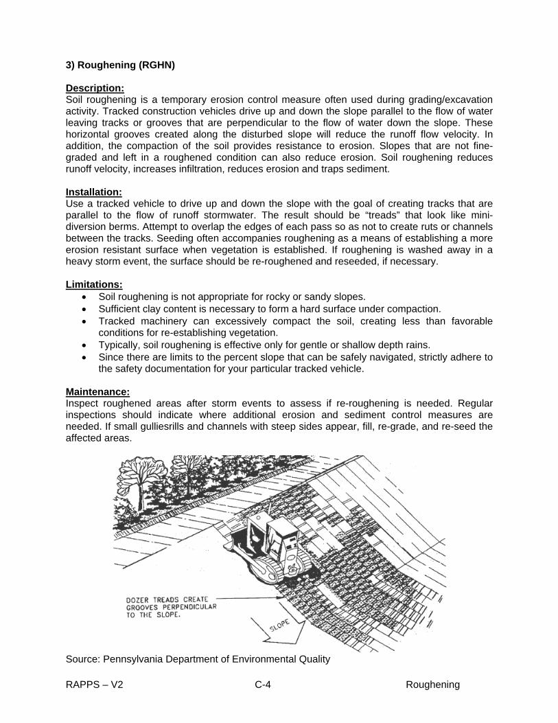
3) Roughening (RGHN) Description: Soil roughening is a temporary erosion control measure often used during grading/excavation activity. Tracked construction vehicles drive up and down the slope parallel to the flow of water leaving tracks or grooves that are perpendicular to the flow of water down the slope. These horizontal grooves created along the disturbed slope will reduce the runoff flow velocity. In addition, the compaction of the soil provides resistance to erosion. Slopes that are not fine-graded and left in a roughened condition can also reduce erosion. Soil roughening reduces runoff velocity, increases infiltration, reduces erosion and traps sediment. Installation: Use a tracked vehicle to drive up and down the slope with the goal of creating tracks that are parallel to the flow of runoff stormwater. The result should be “treads” that look like mini-diversion berms. Attempt to overlap the edges of each pass so as not to create ruts or channels between the tracks. Seeding often accompanies roughening as a means of establishing a more erosion resistant surface when vegetation is established. If roughening is washed away in a heavy storm event, the surface should be re-roughened and reseeded, if necessary. Limitations:
• Soil roughening is not appropriate for rocky or sandy slopes. • Sufficient clay content is necessary to form a hard surface under compaction. • Tracked machinery can excessively compact the soil, creating less than favorable
conditions for re-establishing vegetation. • Typically, soil roughening is effective only for gentle or shallow depth rains. • Since there are limits to the percent slope that can be safely navigated, strictly adhere to
the safety documentation for your particular tracked vehicle. Maintenance: Inspect roughened areas after storm events to assess if re-roughening is needed. Regular inspections should indicate where additional erosion and sediment control measures are needed. If small gulliesrills and channels with steep sides appear, fill, re-grade, and re-seed the affected areas.
Source: Pennsylvania Department of Environmental Quality
RAPPS – V2 C-4 Roughening
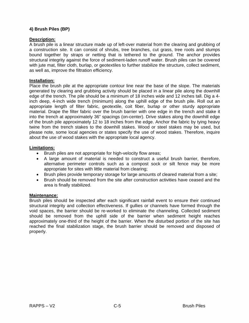
4) Brush Piles (BP) Description: A brush pile is a linear structure made up of left-over material from the clearing and grubbing of a construction site. It can consist of shrubs, tree branches, cut grass, tree roots and stumps bound together by straps or netting that is tethered to the ground. The anchor provides structural integrity against the force of sediment-laden runoff water. Brush piles can be covered with jute mat, filter cloth, burlap, or geotextiles to further stabilize the structure, collect sediment, as well as, improve the filtration efficiency. Installation: Place the brush pile at the appropriate contour line near the base of the slope. The materials generated by clearing and grubbing activity should be placed in a linear pile along the downhill edge of the trench. The pile should be a minimum of 18 inches wide and 12 inches tall. Dig a 4-inch deep, 4-inch wide trench (minimum) along the uphill edge of the brush pile. Roll out an appropriate length of filter fabric, geotextile, coit fiber, burlap or other sturdy appropriate material. Drape the filter fabric over the brush barrier with one edge in the trench and stake it into the trench at approximately 36” spacings (on-center). Drive stakes along the downhill edge of the brush pile approximately 12 to 18 inches from the edge. Anchor the fabric by tying heavy twine from the trench stakes to the downhill stakes. Wood or steel stakes may be used, but please note, some local agencies or states specify the use of wood stakes. Therefore, inquire about the use of wood stakes with the appropriate local agency. Limitations:
• Brush piles are not appropriate for high-velocity flow areas; • A large amount of material is needed to construct a useful brush barrier, therefore,
alternative perimeter controls such as a compost sock or silt fence may be more appropriate for sites with little material from clearing;
• Brush piles provide temporary storage for large amounts of cleared material from a site; • Brush should be removed from the site after construction activities have ceased and the
area is finally stabilized. Maintenance: Brush piles should be inspected after each significant rainfall event to ensure their continued structural integrity and collection effectiveness. If gullies or channels have formed through the void spaces, the barrier should be re-worked to eliminate the channeling. Collected sediment should be removed from the uphill side of the barrier when sediment height reaches approximately one-third of the height of the barrier. When the disturbed portion of the site has reached the final stabilization stage, the brush barrier should be removed and disposed of properly.
RAPPS – V2 C-5 Brush Piles

Source: Virginia Erosion and Sediment Control Handbook, 3rd Edition, 1992
RAPPS – V2 C-6 Brush Piles

5) Straw Bale Barrier (SBB)
Description: Straw or hay bales have been used on construction sites for erosion and sediment control for many years. They are often used as check dams, inlet protection, outlet protection, and perimeter control. Many applications of straw bales for erosion and sediment control are proving ineffective due to the nature of straw bales, inappropriate placement, inadequate installation, or a combination of all three factors (Fifield, 2005). In addition, straw bales are maintenance-intensive and can be expensive to purchase. Because many applications of straw and hay bales have been ineffective, EPA and other agencies recommend that other RAPPS be carefully considered before considering the use of straw bales.
Installation: A shallow (minimum 4-inch deep) bale-sized trench should be excavated and the bales placed in them, end-to-end. The bales should be anchored with stakes (see diagram for placement). Wood or steel stakes may be used, but please note, some local agencies or states specify the use of wood stakes. Therefore, inquire about the use of wood stakes with the appropriate local agency.
Limitations: • Straw bale installations have a high failure rate; • Straw bale installations are seldom designed, installed, and maintained properly; • Straw bales are difficult to transport and to carry around on-site, especially when
attempting to dispose of them when they are waterlogged; • The bindings break and the straw can wash into storm drains, causing clogging; • Straw bales will rot and fall apart over time, especially in areas of high rainfall, and
therefore require intensive maintenance; they commonly last for approximately three months;
• Straw bales will float and therefore must be properly staked even in low flow conditions; • In high flow conditions, the water will flow around a straw bale barrier or undercut spaces
between the bales; • Straw bales may introduce undesirable non-native plants to the area if there are seeds in
the bales.
Maintenance: Straw bales degrade, and rotting bales will need to be replaced on a regular basis (as often as every 3 months depending on local conditions). Erosion from washouts around the bales will need to be repaired. Sediment that settles in ponded areas around correctly installed bales will need to be cleaned out when the sediment accumulation reaches one-third of the bale height. Straw bales will also have to be removed when they burst open or are no longer needed.
RAPPS – V2 C-7 Straw Bale Barrier

Source: NCTCOG Construction BMP Manual, 1998
RAPPS – V2 C-8 Straw Bale Barrier

6) Silt Fence (SF) Description: Silt fences are meant to reduce the velocity of runoff water, thereby allowing the deposition of eroded soil in an up-gradient position from the silt fence. The fence itself consists of a length of silt fence fabric mounted between anchor posts (steel posts are recommended). There are two varieties of fence including: 1) with steel wire reinforcement and 2) without reinforcement. Installation: Installation is initiated by creating a six-inch deep trench along the length of the contour line where the fence is to be placed. The posts are placed at regular intervals, which vary based upon whether or not it is reinforced fence. The generally accepted practice for each variety consists of no more than 6-foot spacing for silt fence without reinforcement and no more than 10-foot spacing for extra strength wire reinforced fencing. The fence post should be driven to 16 to 24 inches above the ground surface and the length of the post varies with the strength of the post material used. Steel stakes should be at least one pound per linear foot of length, and driven at least one third their height into the ground. When hard wood stakes (like oak) are used, they should be a minimum of 2-inch diameter. When soft wooden stakes are used, a larger diameter should be specified (some documents recommend minimum 4-inch diameter and 5 foot length). Drive the stakes along, but just downhill of, the 6-inch deep trench. Stretch the silt fence across the posts leaving no gaps between new portions of fence. When a new roll must be started or ended, secure both ends to the same post. Bury the bottom tail of the fence in the 6-inch deep trench and backfill the trench with the material excavated from the trench. Limitations:
• Installing silt fences along rocky areas or other hard surfaces will prevent uniform anchoring of the fence posts and entrenching the silt fence fabric;
• Silt fences are not suitable for areas where large amounts of concentrated runoff are likely;
• The fence can be overloaded and bend under the pressure created by concentrated stormwater flows;
• Open, windy areas present a problem because high winds can rapidly deteriorate the silt fence.
Maintenance: Inspect silt fences regularly and frequently, no less than every two weeks and after each rainfall event to make sure that they are intact and that there are no gaps where the fence meets the ground or tears along the length of the fence. If you find gaps or tears, repair or replace that section of fabric immediately. Remove the collected sediment from the base of the silt fence when the sediment reaches one-third the height of the fence. Remove sediment more frequently if the collected sediment is creating obvious strain on the fabric and the fence might fail from an intense storm event. When the silt fence is removed, the collected sediment should be removed as well.
RAPPS – V2 C-9 Silt Fence

Source: NCTCOG Integrated Storm Water Managment (iSWM) manual, 2003
Properly installed silt fence along a disturbed slope. Note the use of vegetated buffer and the tight spacing of posts. Source: EPA Storm Water - Menu of BMPs, 2004
RAPPS – V2 C-10 Silt Fence

7) Rock Berm (RB) Description: Rock berms are meant to reduce the velocity of runoff water, thereby allowing the deposition of eroded soil. The berm itself consists of a length of large diameter rocks placed in a linear pile either held in place by gravity or by gabion/chain link fencing. Therefore, there are two varieties of rock berm including: 1) rock berms without wire reinforcement, and 2) rock berms with wire reinforcement. Either variety can be wrapped in filter fabric to add to the filtration capacity of the berm. Installation: Installation is initiated by creating a three to four-inch deep trench along the length of the contour line where the fence is to be placed. The generally accepted minimum rock diameter is four-inches. The minimum width of the berm top (peak) dimension is 24 inches, the minimum width of the base must be wider than the peak but is limited by the natural slope the rock forms when piled up. Therefore, the minimum width of the trench is 36 inches. If fabric is to be used, line the trench with the filter fabric, leaving enough of the fabric out of the trench to cover or wrap the berm’s uphill side. If enough fabric was used to wrap the entire circumference of the berm, then secure the loose end directly to the ground by staking it to the ground. If only the front side was covered, then pull the fabric tight and tether the edges to stakes. The stakes should be placed on the downhill side of the berm and stake spacing should be a maximum of one every 6 to 8 feet.
Limitations:
• Installing rock berms along rocky areas or other hard, uneven surfaces will prevent uniform “seating” of the rock berm base and it becomes difficult to tether the fabric;
• Rock berms are not suitable for areas where large amounts of concentrated runoff are likely, due to the high probability of under-cutting or over-topping of the berm;
• The berm can be overloaded and re-direct stormwater flows around the structure. Maintenance: Inspect rock berms regularly and frequently, no less than every month, as well as after each rainfall event, to make sure that berm has not been breached or undercut. If you find erosion or break-throughs, repair or replace that section of the berm or the base under the berm immediately. Remove the collected sediment from the base of the rock berm when the sediment reaches one-third the height of the berm. Remove sediment more frequently if the collected sediment is creating a ramp of silt and the runoff can over-top the berm. When the rock berm is removed (the fabric, posts & stone) the collected sediment should be removed as well.
RAPPS – V2 C-11 Rock Berm

Source: NCTCOG Construction BMP Manual, 1998
RAPPS – V2 C-12 Rock Berm

8) Diversion Dikes: (DD)
Description: A diversion dike is a berm usually consisting of a compacted earth or base material dike constructed along the perimeter or prior to a disturbed area of a construction site. It is often accompanied by a vegetated ditch or swale, at the top or base of a sloping disturbed area. Depending on its location and the topography of the landscape, a diversion dike can achieve significant re-direction of stormwater. When installed on the up-gradient side of a site, diversion dikes help to prevent stormwater runoff from entering the disturbed portion of a construction site. It can reduce the total amount of sheet flow runoff traveling across the disturbed area and thereby lessen erosion on the site. Diversion dikes can also be located on the down-gradient side of a site. In this case they would be used to divert sediment-laden runoff generated from the disturbed area to onsite sediment-trapping devices, preventing soil loss from the disturbed area.
Installation: Determine the appropriate contour line for the berm to follow so as not to deflect the water more than 30 degrees at a time. Then place and compact some of the excavated native material along the contour line forming a minimum two-foot wide base berm. Placement of silt fences or small stone check dams approximately ten feet prior to deflecting water may help conserve the structural integrity of the dike. Direct diversion dike runoff to sediment-trapping devices, where sediment can settle out of the runoff before it is discharged. Sediment-trapping devices that work with temporary diversion structures include sediment basins, sediment chambers/filters, filter bags, traps, swales and any other structures designed to allow sediment to be collected for proper disposal.
Limitations: • Transforms sheet flow runoff into concentrated flow, which has a higher erosion potential
than sheet flow. Maintenance: Inspect earthen diversion dikes after each rainfall to ensure continued effectiveness. Maintain dikes at their original height. Repair any decrease in height due to settling or erosion immediately. To remain effective, earth dikes must be compacted at all times. Regardless of rainfall frequency, inspect dikes at least once every 2 weeks for evidence of erosion or deterioration.
RAPPS – V2 C-13 Diversion Dikes

Source: NCTCOG Integrated Storm Water Management (iSWM) Manual, 2003
RAPPS – V2 C-14 Diversion Dikes

9) Interceptor Swale (IS) Description: An interceptor swale is typically a v-shaped water collection channel that controls the direction of runoff. This control measure can be used to divert “clean” runoff away from a disturbed area or it can capture sediment laden runoff to a sediment pond or other sediment filtration measure or sediment-removing RAPPS. These swales are typically lined with native grasses, erosion control matting or compacted base. Installation: The swale can be excavated by tilting the blade of the excavator to a sharp angle and dragging the angled blade through the path designed for the swale. The excavator should plan ahead to insure the appropriate (shallow) elevation change from start of the swale to the end of the swale. Please see the drawing below and adjust for site conditions. Limitations:
• Transforms sheet flow runoff into concentrated flow; • May not be suitable for site conditions on the slope (either too steep or too shallow); • Must be stabilized quickly or the swale will contribute to erosion, by shedding it’s soil
lining; • May not be suitable for slopes greater than 5%.
Maintenance: It is recommended that the swale be inspected at least every two weeks or after every rainfall event of 0.5 inches or more. Locate and repair erosion or other damage to the channel. Clear collected sediment and debris to prevent diminished capacity and to prevent discharge of collected material.
RAPPS – V2 C-15 Interceptor Swale

Source: NCTCOG Integrated Storm Water Management (iSWM) Manual, 2003
RAPPS – V2 C-16 Interceptor Swale

RAPPS – V2 C-17 Erosion Control Mat
10) Erosion Control Mat/Geotextiles (ECM)
Description: Erosion control mats and geotextiles are porous fabrics also known as filter fabrics, jute yarn, synthetic fabrics, construction fabrics, or simply fabrics. Mulch mattings are jute or other wood fibers that have been formed into sheets and are more stable than normal mulch. Netting is typically made from jute, wood fiber, plastic, paper, or cotton and can be used to hold the mulching and seeds to the ground. Netting can also be used alone to stabilize soils while the plants are growing; however, it does not retain moisture or temperature well. Mulch binders (either asphalt or synthetic) are sometimes used instead of netting to hold loose mulches together. Geotextiles can aid in plant growth by holding seeds, fertilizers, and topsoil in place.
Installation: Generally, erosion control mats will come with a set of manufacturer specific instructions, and the general principals of installation are listed below. Bury the top of the ECM in a six-inch deep trench and roll the ECM down the slope, instead of across the slope. Overlap the edges of each roll of ECM and staple or anchor the edges of the ECM. Seed and fertilize the ECM itself or the disturbed area prior to covering the slope.
Limitations:
• Geotextiles (primarily synthetic types) have the potential disadvantage of disintegrating when exposed to light;
• Some geotextiles might increase runoff or blow away if not firmly anchored; • Depending on the type of material used, geotextiles might need to be disposed of in a
landfill, making them less desirable than vegetative stabilization; • If the geotextile fabric is not properly selected, designed, or installed, its effectiveness
may be reduced drastically; • More expensive than most non-chemical forms of erosion control.
Maintenance Inspect geotextiles at least monthly to determine if cracks, tears, or breaches have formed in the fabric; if so, repair or replace the damaged portion of fabric immediately. It is necessary to maintain contact between the ground and the mat at all times. Remove trapped sediment as it is discovered.

RAPPS – V2 C-18 Erosion Control Mat
Source: North American Green Erosion Control, 2006

10) Fiber Rolls/Logs (FR)
Description: Fiber rolls (also called Excelsior logs, fiber logs or straw wattles) are tube-shaped erosion-control devices filled with straw, flax, rice, coconut fiber material, or composted material. Each roll is wrapped with a UV-degradable polypropylene netting for longevity or with 100 percent biodegradable materials like burlap, jute, or coir. Fiber rolls complement permanent best management practices used for source control and re-vegetation. Fiber rolls also help to slow, filter, and spread overland flows.
Installation: On slopes, install fiber rolls along the contour with a slight downward angle at the end of each row to prevent ponding at the midsection (California Straw Works, 2005). Turn the ends of each fiber roll up-gradient to prevent runoff from flowing around the roll. Install fiber rolls in shallow trenches dug 3 to 5 inches deep for soft, loamy soils and 2 to 3 inches deep for hard, rocky soils. Determine the vertical spacing for slope installations on the basis of the slope gradient and soil type. According to a manufacturer of this type of erosion control measure, a good rule of thumb is as follows:
1:1 slopes = 10 feet apart
2:1 slopes = 20 feet apart
3:1 slopes = 30 feet apart
4:1 slopes = 40 feet apart
For soft, loamy soils, place the rows closer together. For hard, rocky soils, place the rows farther apart. Stake fiber rolls securely into the ground and orient them perpendicular to the slope. Biodegradable wood stakes or willow cuttings are recommended. Drive the stakes through the middle of the fiber roll and deep enough into the ground to anchor the roll in place. About 3 to 5 inches of the stake should stick out above the roll, and the stakes should be spaced 3 to 4 feet apart. A 24-inch stake is recommended for use on soft, loamy soils. An 18-inch stake is recommended for use on hard, rocky soils.
Limitations: • Fiber rolls are not effective unless entrenched and properly staked, because fiber rolls
can be transported by high flows; • Fiber rolls can be difficult to move once saturated; • To be effective, fiber rolls at the toe of slopes greater than 5:1 must be at least 20 inches
in diameter; • Fiber rolls have a limited sediment capture zone; • Fiber rolls should not be used on slopes subject to creep, slumping, or landslide.
Maintenance: Bi-weekly inspection is recommended to ensure that the rolls remain firmly anchored in place and are not crushed or damaged by traffic. Monitor fiber rolls daily during prolonged rain events. Repair or replace split, torn, unraveled, or slumping fiber rolls. Fiber rolls are typically left in place on slopes. If they are removed, collect and dispose of the accumulated sediment.
RAPPS – V2 C-19 Fiber Rolls/Logs
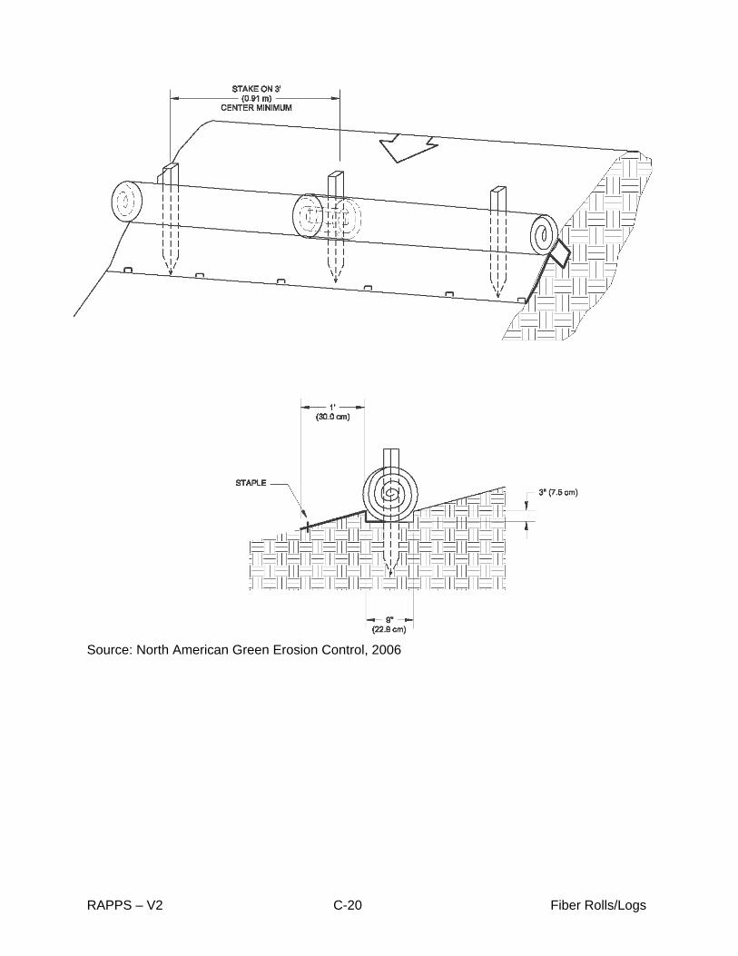
Source: North American Green Erosion Control, 2006
RAPPS – V2 C-20 Fiber Rolls/Logs

Fiber rolls along a newly-vegetated hillside. Note the disturbed slope at the top of the hill Source: EPA Storm Water.Menu of BMPs, 2004
RAPPS – V2 C-21 Fiber Rolls/Logs

11) Compost Sock (CS) Description: A compost sock is a type of compost filter berm that is enclosed in a netting or filter fabric tube, so as to prevent the loss of compost filling and collected sediment. It is a mesh tube filled with composted material that is anchored to the ground perpendicular to the direction of runoff to retain sediment from disturbed areas. The filter sock can be used in place of a traditional erosion control barrier such as a silt fence or straw bale barrier. They should be placed either at the edge of downhill slopes or at intervals along the slope to reduce the velocity and retain sediment. Composts in the sock are generally composed of various organic materials including: manure, yard wastes, wood wastes, and even other bio-degradable wastes. Installation: Compost socks are typically assembled in-the-field by tying a knot in one end of the sock and filling the sock with the composted material. Longer socks are usually filled by using a pneumatic blower. The other end of the sock is knotted shut after the appropriate length is reached. A filter sock the length of the slope is normally used to ensure that runoff does not pass through at the intersection of socks placed end-to-end. If this is not possible, the socks are placed end-to-end along a slope and the ends are anchored together. Wooden stakes may be used to anchor the sock at a post spacing at a maximum of ten feet, and driven into the ground at least six inches. Stakes should have a minimum diameter of 2 inches and the sock should be tied to the stakes rather than driving the stake through the sock itself. Limitations:
• If punctured, the compost can “leak out”, thereby, contributing to the transportation of sediment;
• The sock will act as a filter and actually collect soil from the runoff. If not regularly cleaned, it can clog or deposit a “ramp” of soil causing runoff to go over the top of or around the sock.
Maintenance: Regular inspections are required to insure that the socks are anchored firmly and that there is no “breakthrough” of stormwater under or between socks. Inspections should occur at a minimum of every two weeks and after each rainfall event of over 0.1 inches.
RAPPS – V2 C-22 Compost Sock

Compost Socks staked in place along a storm water swale. Source: Ohio Department of Transportation, 2008
RAPPS – V2 C-23 Compost Sock
12) Sediment Basin (SB)
Description: Sediement basins (also known as a rock dam or rock dam pond) can be used to capture sediment from stormwater runoff before it leaves a construction site. They allow a pool to form in an excavated or natural depression, where sediment can settle. The pool is dewatered through a single riser and drainage hole leading to a suitable outlet on the downstream side of the embankment or through the gravel of the rock dam. The water is released by the pipe more slowly than it would be without a control structure.
Installation: It is impossible to provide a one-size fits all design approach in this manual. Preferably a civil engineer or a certified erosion and sediment control professional should be retained to design the basin. In general, a sediment basin is constructed by excavation or by erecting an earthen embankment across a low area or drainage swale. The basin can be temporary or permanent. Some sediment basins are designed to drain completely during dry periods. Others are constructed so that a shallow pool of water remains between storm events. Limitations:
• A sediment basin with an earthen embankment or a rock dam should not be used in an area of continuously running water (live streams);
• A sediment basin is not recommended in an area where failure of the earthen or rock dam will result in loss of life or damage to homes, buildings, utilities or roads;
• The expense related to the design and construction of a sediment basin may be high compared to other erosion control measures.
Maintenance: Routine inspection and maintenance of sediment basins is essential to their continued effectiveness. Inspect basins after each storm event and bi-weekly to ensure proper drainage from the collection pool and the need for structural repairs. Replace material eroded from earthen embankments or stones moved from rock dams as soon as discovered. Locate sediment basins in an area that is easily accessible to maintenance crews for the removal of accumulated sediment. Dewater and remove sediment from the basin when the storage capacity has reached approximately 50 percent. Remove collected trash and large debris from around dewatering devices promptly after rainfall events.
RAPPS – V2 C-24 Sediment Basin

Source: NCTCOG Integrated Storm Water Managment (iSWM) Manual, 2003
RAPPS – V2 C-25 Sediment Basin

D-1
APPENDIX D. EXAMPLES OF SPECIALTY RAPPS
1) Stabilized Construction Entrance: (SCE) Description: Stabilized construction entrances limit the amount of tracked materials (mud and dust) from leaving the construction site. Mud and sediment are removed from vehicle tires when leaving the site as tires pass over rock pad. A “cattle-guard” grate or similar structure may be added to further remove mud from the tires. In addition, a wheel wash area may be added to clean tires and drain runoff to a dewatering pit or a filter bag. Installation: Install SCE at entrances/exits to paved roads and place geotextile filter fabric under medium to large diameter crushed rock. The length and width of the entrance should be adequate to allow large vehicles to access site. See drawing below and adjust to site conditions. Limitations:
• Less effective with increased rain and mud; • Additional sweeping of paved road will be necessary; • Removal necessary after completion of construction; • Availability of rock.
Maintenance: A stone construction entrance must be regularly inspected after each 0.5-inch rainfall event to determine if the mud and silt collected has covered the stone surface of entrance. When the aggregate is clogged with sediment, the SCE should be replaced or washed down into a sediment collecting structure. If ponding occurs in low areas of the pad, the stone should be replaced.
RAPPS – V2 D-2 Road Surface Slope
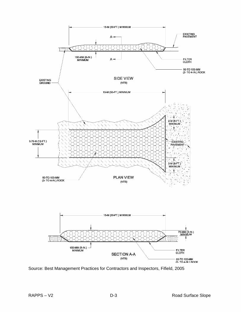
Source: Best Management Practices for Contractors and Inspectors, Fifield, 2005
RAPPS – V2 D-3 Road Surface Slope

2) Road Surface Slope (RDSS): Description: This technique requires sloping the road surfaces toward constructed channels parallel to the roads. The ditches convey concentrated runoff of surface water from roads and surrounding areas to a stabilized area. Installation: Slope the road toward channels parallel to the road. Excavate channel along the roadside to a width and depth that can convey expected flows. Slope the ditches so that water velocities do not cause excessive erosion. Shape and level ditches removing excess spoil so water can flow. Vegetate or line ditches with material to prevent erosion Limitations:
• Erosion occurs from the road surface or road side ditch, causing potholes; • Road surface slopes do not necessarily filter sediment from runoff
Maintenance: Monthly inspections should be conducted to prevent depressions or erosion of the crown or slope. If the road base has collapsed or washed-out, the surface will form potholes and depressions. Repair the road and base in the affected section as soon as practicable after discovery.
Source: Modified from RAPPS Version 1.0, IPAA, 2004
RAPPS – V2 D-4 Road Surface Slope

3) Drainage Dips: (DIP) Description: A drainage dip is an intentional depression in the roadway, usually consisting of a compacted earth or base material “swale” that drains water from the roadway instead of allowing it to puddle and erode the surface of the road. It will typically drain to a roadside ditch. Installation: During road grading provide a small grade change over a 10-foot stretch of roadway and then grade the next 10-foot section of roadway back to the original elevation, causing a dip over 20 linear feet. The dip should be angled to one or both edges of the road, but with medium-sized rip-rap placed at the edge of the road, thereby providing some erosion protection for the road’s base. Limitations:
• Generates point source of runoff water from the road surface. Maintenance: Inspect after each rainfall and re-compact the roadbase as needed.
Source: Modified from RAPPS Version 1.0, IPAA, 2004
RAPPS – V2 D-5 Drainage Dips

4) Road-Side Ditches: (RDSD) Description: This technique requires constructing channels parallel to roads. The ditches convey concentrated runoff of surface water from roads and surrounding areas to a stabilized area. Installation: Excavate a channel along the roadside to a width and depth that can handle expected flows. Slope channels so that water velocities do not cause excessive erosion. Shape, level and line the channel, with rip-rap, erosion control mat or vegetation to prevent erosion. Limitations:
• Erosion occurs within channel; • Channel does not necessarily filter sediment from runoff.
Maintenance: Inspect after each rainfall greater than 0.5 inches in order to assure the stability of the roadbase.
Source: Modified from RAPPS Version 1.0, IPAA, 2004
RAPPS – V2 D-6 Road-Side Ditches

5) Turnouts or Wing Ditches: (TO) Description: These structures are extensions of road-side ditches and will effectively remove run-off water from the ditch into well-stabilized areas. Installation: Slope the turnout gradually down from the bottom of the road ditch and angle the turnout at approximately 30° to the road ditch. Discharge the turnout into a well-vegetated area or install a form of secondary control such as rock filter or straw bales. Space the turnouts according to slope. Limitations:
• Gradual slopes only; • Require vegetative cover or other filter at discharge point.
Maintenance: Inspect after each rainfall greater than 0.5 inches in order to assure the stability of the turnout.
RAPPS – V2 D-7 Turnouts or Wing Ditches

6) Cross Drain Culverts: (CULV) Description: This technique can be used to direct road-side ditch flow across a road or may be used to direct stream flow under a road or construction area. Culverts passing construction sites will allow for continued flow of stream with minimal siltation. Installation: Culverts may be steel, aluminum, or concrete and should be placed at surface grades to allow normal low-flow water to be conveyed. Soil or road base should be compacted over culverts to a minimum of 12 inches. Culvert size should be adequate to convey anticipated flow. A ditch plug will be required within the road-side ditch to direct water into the culvert. The culvert grade change should be adequate to convey expected flow rates. Increase the frequency of culverts with increased slope. Rock rip-rap is commonly required at the outlet of the culvert. Limitations:
• Culverts may become clogged; • Culverts are not a sediment filters and will likely transport silt; • Some silt may collect at the entrance of the culvert only to be transported subsequent
rain events. Maintenance: Inspect the road base after each rainfall event greater than 0.5 inches to insure that it has not been eroded. Replace the eroded material as soon as practical.
RAPPS – V2 D-8 Cross Drain Culverts

7) Sediment Traps: (ST) Description: This technique uses a basin or pond to hold sediment-laden water so that sediment can settle and water is absorbed into the soil. Sediment traps are useful for construction sites where excessive runoff will need to be captured and filtered and other RAPPS are insufficient. Installation: Excavate the sediment trap or basin within an area where runoff may be easily directed. The side slopes should be 2:1 or flatter and machine compacted. The volume of the sediment trap should have a minimum 2-year storm event capacity and allow for water infiltration. Construct a spillway or outfall structure with rock rip-rap at the outlet. Limitations:
• Not for use in rocky situations; • Overflow can result during large rainfall events; • Water will remain in the sediment trap for extended periods.
Maintenance: Inspect bi-weekly or after each rainfall event of 0.5 inches or more. Remove sediment when it reaches 50% capacity.
Source: NCTCOG Integrated Storm Water Management (iSWM) Manual, 2003
RAPPS – V2 D-9 Sediment Traps

8) Construction Mats: (CM) Description: This technique spreads the weight of construction equipment over a broad area to help prevent soil compaction and soil exposure. Installation: Mats are constructed of large timber fitted, tied or bolted together. Mats are placed ahead of, or under operating equipment to provide a stable work area. Limitations:
• Useful on wet, soggy, and/or inundated soils; • Mats are bulky and difficult to move; • Does not filter sediment from runoff.
Maintenance: Damage to the mat may occur due to heavy traffic and should be inspected once per month for damage.
Source: Carolina Mat Incorporated, 2008
RAPPS – V2 D-10 Construction Mats

9) Filter Bags: (FB) Description: A filter bag is an outlet structure from a sediment laden pond or trap, usually connected to a floating pump or as an exit to a drain. Installation: Follow the bag’s manufacturer’s directions for sealing the bag and loading it with the appropriate volumetric flow rate (CFM). Limitations:
• It must be replaced regularly; • It is part of a system of controls and not a stand-alone device; • It must be monitored regularly for overloading.
Maintenance: Inspect after every rain event or at least every two weeks for overloading. Replace the bag, as needed.
RAPPS – V2 D-11 Filter Bags

D-12 Filter Bags
RAPPS – V2
Source: Best Management Practices for Contractors and Inspectors, Fifield, 2005

10) Trench Dewatering and Discharge: (TDD) Description: Trench dewatering and discharge is a method more than a structure and usually consists of draining a diked area or trench with a pump and filter bag surrounded by a straw bale berm (or better) containment that provides additional filtration for the discharged water. Installation: See drawing and adjust for site conditions. Limitations:
• It must be maintained very regularly; • It is a temporary solution for removing water from a trench.
Maintenance: Inspect after each use and replace the berm or bag as capacity is diminished, or as needed.
Source: Modified from RAPPS Version 1.0, IPAA, 2004 RAPPS – V2 D-13 Trench Dewatering And Discharge

RAPPS – V2 D-14 Dewatering Structure
11) Dewatering Structure: (DS) Description: A dewatering structure is a berm usually consisting of a straw bale or compost filter dike surrounding an open pipe from a pond or other silt containment structure. It is meant as a final filtration step and not as a stop-gap last line-of-defense measure. Large amounts of silt should not be sent to this structure. Installation: See figure and adjust for site conditions.
Limitations:
Maintenance: Inspect weekly or after each discharge event.
• Not effective for large flows or heavy silt-laden water ; • Straw bales will clog eventually causing ponding and submerged discharge pipe; • Straw bales must be replaced very regularly to prevent rotting or clogging.
Source: Modified from RAPPS Version 1.0, IPAA, 2004

12) Typical Open Cut Flowing Stream Crossing Flume Pipe: (SCFP) Description: Usually consisting of a flume pipe that drains moving water over an open trench. It is meant as a temporary measure and is dangerous to the life of personnel if they are to be working in the trench. Take extreme precaution in the use of this measure to prevent cave-ins and the escape of the flumed water. Installation: See drawing and adjust to site conditions Limitations:
• Temporary; • Dangerous to personnel working in the trench, especially if rain events increase the
water flow above the capacity of the flume. Maintenance: Inspect daily and after rain events.
Source: Modified from RAPPS Version 1.0, IPAA, 2004
RAPPS – V2 D-15 Typical Open Cut Flowing Stream Crossing Flume Pipe

13) Typical Open Cut Minor Flowing Stream Crossing Dam and Pump: (SCDP) Description: A method usually consisting of a diversion dike or berm made up of: sand bags, compacted earth or base material dike. A pump and discharge hose are used to convey water downstream. Installation: See drawing and adjust to site conditions Limitations: • Temporary; • Personnel must be protected from overflows. Maintenance: Inspect daily and after each rain event.
Source: Modified from RAPPS Version 1.0, IPAA, 2004
RAPPS – V2 D-16 Typical Open Cut Minor Flowing Stream Crossing Dam and Pump

14) Post Construction Stream Bank Stabilization: (SBS) Description: Stabilization usually consisting of a compacted earth or rip-rap material over geotextiles. Installation: See drawing and adjust to site conditions Limitations: • Vegetative stabilization is preferred and is considered more permanent Maintenance: Inspect after each rainfall event larger than 0.5 inches
Source: Modified from RAPPS Version 1.0, IPAA, 2004RAPPS – V2 D-17 Post Construction Stream Bank Stabilization

15) Typical Open Cut Dry Stream Crossing: (DSC) Description: A diversion dike is used to separate the spoil pile from the open trench and waterway (creek). Installation: See drawing and adjust to site conditions Limitations:
• Water bodies should be treated with extreme care so as not to pollute with spoil. Maintenance: Inspect after each rainfall event larger than 0.5 inches
Source: Modified from RAPPS Version 1.0, IPAA, 2004
RAPPS – V2 D-18 Typical Open Cut Dry Stream Crossing

16) Temporary Equipment Crossing of Flowing Creek (Bridged) (TECFC) Description: Bridged crossing of a creek. Installation: See drawing and adjust to site conditions Limitations:
• Structural integrity of foundation and bridge is the greatest concern and should be evaluated by an experienced P.E. or construction manager.
Maintenance: Inspect after each rainfall event larger than 0.5 inches.
Source: Modified from RAPPS Version 1.0, IPAA, 2004
RAPPS – V2 D-19 Temporary Equipment Crossing of Flowing Creek