tatianav.dogadova, marati.kusainov, vyacheslava.vasilievserdica/inpress/1193.pdf · 2 t. v....
TRANSCRIPT
To appear in Serdica Math. J. 43 (2017) SerdicaMathematical Journal
Bulgarian Academy of SciencesInstitute of Mathematics and Informatics
TRUNCATED ESTIMATION METHOD
AND APPLICATIONS
Tatiana V. Dogadova, Marat I. Kusainov, Vyacheslav A. Vasiliev
Communicated by P. Jagers
Abstract. This paper presents an estimation method of ratio type func-tionals by dependent sample of fixed size. This method makes it possible toobtain estimators with guaranteed accuracy in the sense of the L2m-norm,m ≥ 1.
As an illustration, some parametric estimation problems on a time in-terval of a fixed length are considered. In particular, parameters of lin-ear continuous-time and non-linear discrete-time processes are estimated.Moreover, the parameter estimation problem of non-Gaussian Ornstein–Uhlenbeck process by discrete-time observations with guaranteed accuracyis solved.
In addition to non-asymptotic properties, the limit behavior of presentedestimators is investigated. It is shown that all the truncated estimators haverates of convergence of the estimators they are based upon. These estimatorsare used for the construction of adaptive predictors for dynamical systemswith unknown parameters.
2010 Mathematics Subject Classification: 60G25, 62M20, 60G52, 60J60, 62F12, 93E10.Key words: Adaptive optimal prediction, dynamic systems, autoregressive processes, stochas-
tic differential equations, stochastic differential equations with time delay, risk function; guar-anteed parameter estimation.

2 T. V. Dogadova, M. I. Kusainov, V. A. Vasiliev
The problem of asymptotic efficiency of adaptive one-step predictors forstable discrete- and continuous-time processes with unknown parameters isconsidered. The proposed criteria of optimality are based on the loss func-tion, defined as a linear combination of sample size and squared predictionerror’s sample mean. As a rule, the optimal sample size is a special stoppingtime.
1. Introduction. The main purpose of this paper is to present applica-tions of the truncated estimation method in order to construct optimal adaptivepredictors for the stochastic processes related with discrete and continuous-timedynamical systems. The proposed procedures are based on the so-called truncatedestimators which have been developed in order to estimate ratio type functionalsfrom a wide class by dependent observations and by samples of fixed size so thatthey had guaranteed accuracy in the sense of the L2m-norm, m ≥ 1. Examplesof parameter estimation problems of discrete and continuous time systems on atime interval of a fixed length are considered.
It is shown that truncated estimators may keep asymptotic propertiesof the estimators they are based upon. One of the many useful applications ofestimators with the said quality is adaptive prediction for dynamical systemswith unknown parameters. It is then possible to optimize the risk function whichis a linear combination of sample mean of mean-square deviation of predictorsand sample size. The risk function of such structure was proposed in [3], see alsoreferences therein.
According to Ljung’s concept the prediction is a crucial part in construct-ing complete probabilistic models of dynamical systems (see [24, 25]). A model isconsidered to be useful if it allows to make predictions of high statistical quality.Models of dynamical systems often have unknown parameters, which demandestimation in order to build adaptive predictors. The quality of adaptive predic-tion explicitly depends on the chosen estimators of model parameters. Possibleestimation methods include the classic stochastic approximation, maximum like-lihood, least squares and sequential estimation methods among others. The firstthree methods provide estimators with given statistical properties under asymp-totic assumptions, when the duration of observations tends to infinity (see, e.g.,[1, 36]). The sequential estimation method makes it possible to obtain estimatorswith guaranteed accuracy by samples of finite but random and unbounded size(see, e.g., [4, 9, 15, 16, 17, 18, 23, 27, 29, 30, 33, 34, 35, 37] among others).
Both approaches do not guarantee prescribed estimation accuracy whenusing samples of non-random finite size and lead up to complicated analyticalproblems in adaptive procedures.
Truncated estimation method and applications 3
Results in non-asymptotic parametric and non-parametric problems canbe found in [28, 37] among others. In particular, they investigated non-asymptoticproperties of the LSE-estimator for the scalar first-order autoregressive process.
At the same time, the more modern truncated sequential estimationmethod yields estimators with prescribed accuracy by samples of random butbounded size (see, e.g., [5, 8, 13, 14, 34, 35]). However, at the moment this ap-proach is developed for scalar dynamic systems only. The truncated estimationmethod was introduced in [40] as a modification of the truncated sequential es-timation one. Truncated estimators were constructed for ratio type multivariatefunctionals by samples of fixed size and have guaranteed accuracy in the sense ofthe L2m-norm, m ≥ 1 (see also [41]).
The requirement of both good prediction quality and reasonable durationof observations is formulated as a risk efficiency problem. The criterion is given bycertain loss functions and optimization is performed based on it. The loss functiondescribing sample mean of squared prediction errors and sample size as well asthe corresponding risk was examined in [38, 39] in application to scalar AR(1).Later the results of those papers were refined and extended to other stochasticmodels in [11]. There was considered a risk function defined on the basis ofsquared estimation error of sequential estimator of the dynamic parameter. Amodified stopping rule was proposed, enhancing the result of [38]. In the twopapers on risk efficiency problems mentioned above the least squares estimatorsand sequential estimators of unknown parameters were used.
In this paper we construct and investigate real-time predictors which onlyuse past values of the process. Such an approach leads to some technical diffi-culties but is more closely related to real applications. We consider the problemof minimization of the risk function associated with predictors of values of theprocess and size of a sample. It should be noted that first truncated parameterestimation method was applied for construction of adaptive optimal predictorsof VAR(1) in [22]. Here we apply this method for more complicated stochasticsystems. Among the processes considered are stable multivariate discrete timeAR(1), ARMA(1, 1) and RCA(1), as well as continuous time diffusion and timedelayed processes. The proposed procedure is shown to be asymptotically riskefficient as the cost of prediction error tends to infinity.
2. Truncated estimation method. General results. Let (Ω,F ,P) be a probability space with a filtration Ft in discrete or continuous timeand let ft and gt be Ft-adapted random processes, where ft and gt is s × q-dimensional matrix and scalar function respectively.
4 T. V. Dogadova, M. I. Kusainov, V. A. Vasiliev
Let
(1) ΨT = fT /gT
be an estimator of a matrix Ψ. For instance, the matrix Ψ can be a ratio
Ψ = f/g
and fT and gT are estimators of matrix f and number g respectively.
Consider the following modification of the estimator ΨT :
(2) ΨT (H) = ΨT · χ(|gT | ≥ H),
where H is a function H = HT , defined below and the notation χ(A) means theindicator function of set A.
Our main aim is to formulate general conditions on the processes fT , gTand on the parameter H giving a possibility to estimate Ψ with a guaranteedaccuracy in the sense of the L2m-norm, m ≥ 1.
Define for some ϕT (m), wT (µ), H and g, the function
VT (m,µ,H) =1
H2mϕT (m) +
‖Ψ‖2m(|g| −H)2µ
wT (µ),
as well as for positive integer p < m and a positive monotonously decreasingfunction HT , the function
VT (p) = 22p−1g−2p·(ϕT (p) +H−2p
T · ϕpm
T (m) · wpµ
T (µ)
)+‖Ψ‖2p·(g −HT )
−2µ·wT (µ)
and the time T0 = infT ≥ 0 : HT ≤ |g|.Theorem 2.1. Assume for some values m and µ there exist positive
functions ϕT (m) and wT (µ), decreasing to zero, as well as a value g such thatthe following assumptions hold
(i) E‖fT −ΨgT ‖2m ≤ ϕT (m);
(ii) E(gT − g)2µ ≤ wT (µ).
Then, the estimator ΨT (H) defined in (2) has the following properties
(a) in the case of known number g for every H ∈ (0, |g|)
E‖ΨT (H)−Ψ‖2m ≤ VT (m,µ,H);

Truncated estimation method and applications 5
(b) in the case of unknown g for every (possibly slowly decreasing to zero)positive function H = HT and every positive integer p, satisfying for some m >1 and µ > 1
mp
m− p≤ µ
it holdsE‖ΨT (H)−Ψ‖2p ≤ VT (p), T > T0.
Remark 1. If the number g in Theorem 2.1 is unknown but a positivelower bound g∗ for |g| is known, then the parameter H in the definition of thetruncated estimator (2) should be taken from the interval (0, g∗) and the number|g| in the definition of the function VT (m,µ,H) should be replaced by g∗.
Proof of Theorem 2.1 is similar to the proof of Theorem 1 from [40]formulated for the discrete-time case.
3. Parameter estimation. Examples.3.1. Discrete-time systems.
3.1.1. Estimation of parameters of a stable first order scalar autoregres-sion. Consider the process satisfying the following equation
(3) xn = λxn−1 + ξn, n ≥ 1,
where noises ξn, n ≥ 1 are i.i.d. zero mean random variables with finite (for someeven number γ ≥ 2) moments σ2γ = Eξ2γn , as well as Ex2γ0 < ∞ and |λ| < 1.
Consider the estimation problem of λ and σ2 = Eξ2n with a guaranteedaccuracy.
In what follows, C will denote a generic non-negative constant whosevalue is not critical (and not necessarily the same throughout the paper).
a) Non-asymptotic estimation of λWe define the estimator of the type (2) with T = N on the basis of the
least squares estimator (LSE) of the form (1)
λN =
1N
N∑n=1
xnxn−1
1N
N∑n=1
x2n−1
, N ≥ 1.
According to general notation, in this case we have
Ψ = λ, ΨN = λN ,
6 T. V. Dogadova, M. I. Kusainov, V. A. Vasiliev
fN =1
N
N∑
n=1
xnxn−1, gN =1
N
N∑
n=1
x2n−1
and ΨN = λN ,
(4) λN = λN · χ(gN ≥ H).
Using the equality
gN =σ2
1− λ2+
1
(1− λ2)N
[x20 − x2N + 2λ
N∑
n=1
xn−1ξn +
N∑
n=1
(ξ2n − σ2)
],
which can be obtained from (3), we can find the limit (see [37, 40])
g = limN→∞
gN =σ2
1− λ2Pλ − a.s.
All the conditions of Theorem 2.1 hold, hence– for the case of known σ2 and 0 < H < σ2
(5) Eθ(λN − λ)2m ≤ C(θ)
Nm+
C(θ)
N2m, N ≥ 1;
– for the case of unknown σ2 we put H = (HN ) (e.g., slowly decreasingfunction) from Theorem 2.1 in the definition (4) of the estimator λN and for Nlarge enough, we have
Eθ(λN − λ)2m ≤ C(θ)H2mN
Nm.
Here θ = (λ, σ2, σ2γ).For the parameter estimation with a guaranteed accuracy we have to know
that, e.g., θ ∈ Θ, where Θ = θ = (λ, σ2, σ2γ) : |λ| ≤ r < 1, 0 < σ2 ≤ σ2 ≤ σ2.In this case we can find the known functions
ϕN (m) = supθ∈Θ
ϕN (m, θ) and wN (m) = supθ∈Θ
wN (m, θ)
such thatsupΘ
Eθ(fN − λgN )2m ≤ ϕN (m),
supΘ
Eθ(gN − g)2m ≤ wN (m).

Truncated estimation method and applications 7
In general, for 0 < H < σ2, we have
(6) supΘ
Eθ(λN − λ)2m ≤ C
Nm+
C
N2m, N ≥ 1.
In particular, for γ = 2 and m = 1,
supΘ
Eθ(λN − λ)2 ≤[
(σ2)2
(1− r2)H2+
r2C
(σ2 −H)2
]1
N+
r2C
(σ2 −H)21
N2.
b) Non-asymptotic estimation of σ2
Consider the estimation problem of the noise variance σ2 in the model(3) under the assumption γ = 4 (σ8 < ∞, Ex80 < ∞).
In the definition of the LSE type estimator σ2N defined as
σ2N =
1
N
N∑
n=1
(xn − λNxn−1)2, N ≥ 1,
we use the estimator λN of λ, which is defined in (4) and has known non-asymptotic properties (6) for m = 1 and m = 2.
Thus, we have obtained estimator of σ2 with a guaranteed accuracy:
supΘ
Eθ(σ2N − σ2)2 ≤ C
N, N ≥ 1.
It should be noted, that this estimator is asymptotically equivalent to thecorresponding LSE. In particular, it has optimal rate of convergence as N → ∞.
Full proofs of results of this section can be found in [40].
3.1.2. Estimation of parameters of a stable ARARCH(1,1). Consider theprocess satisfying the following equation
xn = λxn−1 +√
σ20 + σ2
1x2n−1 · ξn, n ≥ 1,
where noises ξn, n ≥ 1 are i.i.d. zero mean random variables with the varianceequal to one and finite fourth moment σ4 = Eξ41 , as well as Ex
40 < ∞.
Define the LSE λN of λ of the form:
λN =
1N
N∑n=1
xnxn−1
1N
N∑n=1
x2n−1
, N ≥ 1,

8 T. V. Dogadova, M. I. Kusainov, V. A. Vasiliev
which is strongly consistent under the following stability condition
(7) λ4 + 6λ2σ21 + (σ2
1)2σ4 < 1.
a) Non-asymptotic estimation of λAccording to general notation, in this case we have
Ψ = λ, ΨN = λN ,
fN =1
N
N∑
n=1
xnxn−1, gN =1
N
N∑
n=1
x2n−1
and ΨN = λN ,
(8) λN = λN · χ(gN ≥ H).
Define for some known numbers r ∈ (0, 1), σ20, σ
20, σ
21, and σ2
1 the set
Θ = θ = (λ, σ20 , σ
21) : λ4+6λ2σ2
1+(σ21)
2σ4 ≤ r, σ20 ≤ σ2
0 ≤ σ20, σ2
1 ≤ σ21 ≤ σ2
1.
Then for 0 < H <σ20
1− σ21
and every N ≥ 1
supΘ
Eθ(λN − λ)2 ≤ 1
H2N+
(1− σ21)
2
(σ20 − (1− σ2
1)H)21
N2.
It should be noted, that the rate of convergence of the obtained upperbound is the same as the rate of the LSE and is optimal.
b) Non-asymptotic estimation of σ20 and σ2
1
We will construct estimators with guaranteed accuracy on the basis ofcorrelation estimators:
1b) of σ20 with known σ2
1 :
σ20(N) =
1
N
N∑
n=1
[x2n − (λ2N + σ2
1)x2n−1];
2b) of σ21 with known σ2
0 :
σ21(N) =
N∑n=1
(x2n − σ20)
N∑n=1
x2n−1
− λ2(N),

Truncated estimation method and applications 9
which are strongly consistent under the condition (7), see, e.g., [26].Define estimators for considered cases
1b) σ20(N) =
1
N
N∑
n=1
[x2n − ((λ∗N )2 + σ2
1)x2n−1];
2b) σ21(N) =
1N
N∑n=1
(x2n − σ20)
1N
N∑n=1
x2n−1
χ(gN ≥ H)− (λ∗N )2,
whereλ∗N = proj[−1,1]λN ,
λN and gN are defined in (8).Similar to the previous sections, the upper bounds for the MSE’s of these
estimators with known constants C0 and C1 can be found
(i) supΘ0
Eθ(σ20(N)− σ2
0)2 ≤ C0
N,
where Θ0 = θ = (λ, σ20) : λ4 + 6λ2σ2
1 + (σ21)
2σ4 ≤ r, σ20 ≤ σ2
0 ≤ σ20 and
(ii) supΘ1
Eθ(σ21(N)− σ2
1)2 ≤ C1
N,
where Θ1 = θ = (λ, σ21) : λ4 +6λ2σ2
1 + (σ21)
2σ4 ≤ r, σ21 ≤ σ2
1 ≤ σ21, r ∈ (0, 1).
Full proofs of results of this section can be found in [40].
3.1.3. Estimation of parameters of a stable first order VAR(1). We applyin this section the presented general truncated method for estimation of matrixparameters in multivariate systems.
Consider the p-dimensional process (p > 1) satisfying the following equa-tion
(9) x(n) = Λx(n− 1) + ξ(n), n ≥ 1,
where noises ξ(n), n ≥ 1 are i.i.d. zero mean random column vectors with thevariance matrix Σ = Eξ(n)ξ′(n) and finite moments of the order 8(p− 1), as wellas E‖x(0)‖8(p−1) < ∞ and the stability condition for the process (9) is satisfied,i.e. all the eigenvalues of the matrix Λ lie in the open unit circle.
It should be noted, that under these conditions there exist finite numbersσ2mx , such that
supn,Λ0
EΛ‖x(n)‖2m ≤ σ2mx , 1 ≤ m ≤ 4(p− 1),

10 T. V. Dogadova, M. I. Kusainov, V. A. Vasiliev
where Λ0 is a compact set from the stable region of (x(n)).Consider the estimation problem of Λ with a guaranteed accuracy.We define the estimator of the type (2) on the basis of the LSE of the
form (1)
ΛN = G−1N ΦN , N ≥ 1,
where
GN =1
NGN , GN =
N∑
n=1
x(n− 1)x′(n− 1),
ΦN =1
NΦN , ΦN =
N∑
n=1
x(n)x′(n − 1), N ≥ 1.
Define the matrix
G+N = ∆NG
−1N , ∆N = det(GN ).
According to the general notation, in this case we have
Ψ = Λ, ΨN = ΛN ,
fN = ΦNG+N , gN = ∆N ,
and ΨN = ΛN ,Λ∗N = ΛN · χ(gN ≥ H).
It is easy to verify that with PΛ-probability one
limN→∞
GN = F and limN→∞
∆N = ∆ > 0,
where F is a positive definite p× p-matrix (see, e.g., [1, 12]).Then
f = Λ∆, g = ∆.
It can be shown, see [40] that there exists a given number C0 such thatfor every N ≥ 1,
supΛ∈Λ0
EΛ‖Λ∗N − Λ‖2 ≤ C0
N,
Λ0 is a compact set from the stable region of the process (9).Consider the case of unknown Λ0.
Define the number N0 = maxp,
⌊e∆
−2⌋
.
Let the truncated estimators ΛN be defined as follows
(10) ΛN = ΛN · χ(∆N ≥ HN ), HN = log−1/2(N + 1).
Truncated estimation method and applications 11
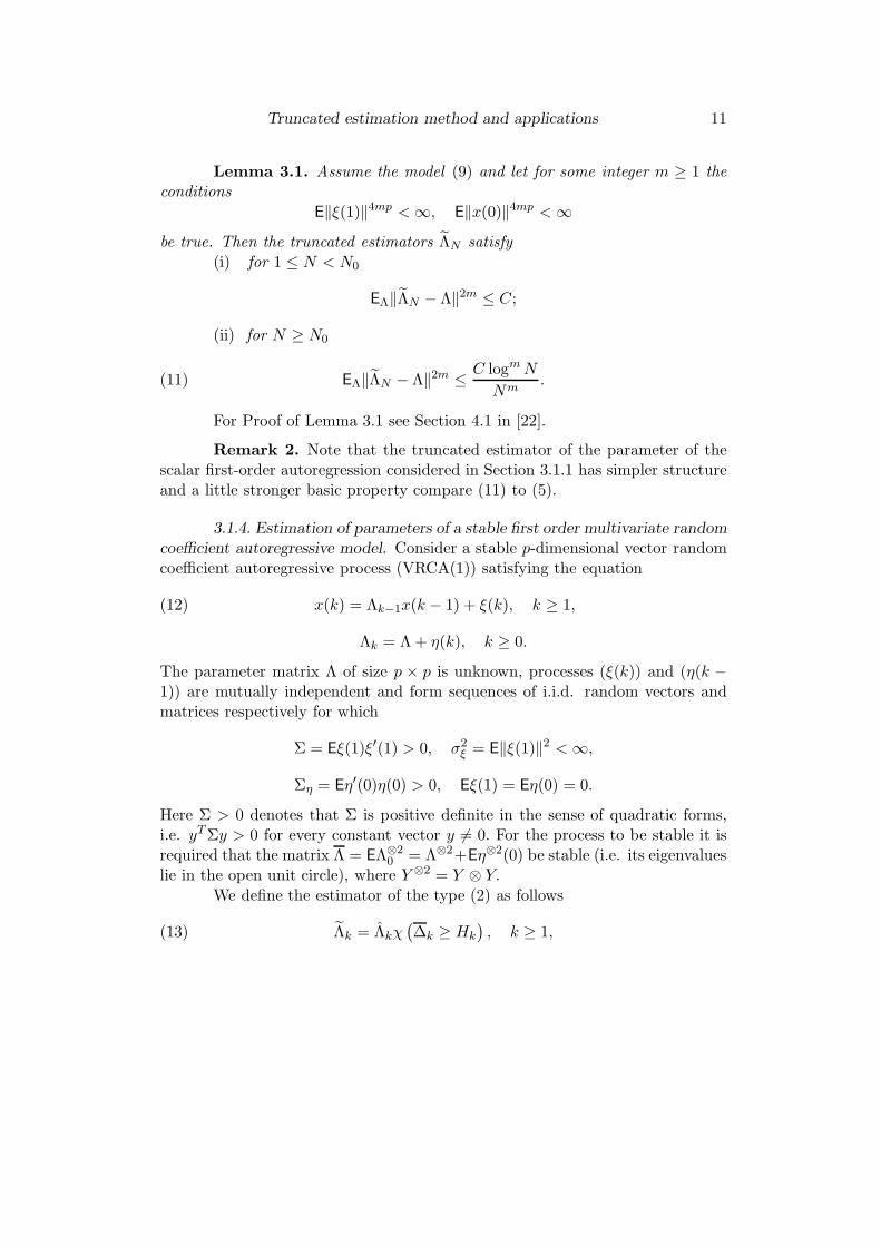
Lemma 3.1. Assume the model (9) and let for some integer m ≥ 1 theconditions
E‖ξ(1)‖4mp < ∞, E‖x(0)‖4mp < ∞be true. Then the truncated estimators ΛN satisfy
(i) for 1 ≤ N < N0
EΛ‖ΛN − Λ‖2m ≤ C;
(ii) for N ≥ N0
(11) EΛ‖ΛN − Λ‖2m ≤ C logmN
Nm.
For Proof of Lemma 3.1 see Section 4.1 in [22].
Remark 2. Note that the truncated estimator of the parameter of thescalar first-order autoregression considered in Section 3.1.1 has simpler structureand a little stronger basic property compare (11) to (5).
3.1.4. Estimation of parameters of a stable first order multivariate randomcoefficient autoregressive model. Consider a stable p-dimensional vector randomcoefficient autoregressive process (VRCA(1)) satisfying the equation
(12) x(k) = Λk−1x(k − 1) + ξ(k), k ≥ 1,
Λk = Λ+ η(k), k ≥ 0.
The parameter matrix Λ of size p × p is unknown, processes (ξ(k)) and (η(k −1)) are mutually independent and form sequences of i.i.d. random vectors andmatrices respectively for which
Σ = Eξ(1)ξ′(1) > 0, σ2ξ = E‖ξ(1)‖2 < ∞,
Ση = Eη′(0)η(0) > 0, Eξ(1) = Eη(0) = 0.
Here Σ > 0 denotes that Σ is positive definite in the sense of quadratic forms,i.e. yTΣy > 0 for every constant vector y 6= 0. For the process to be stable it isrequired that the matrix Λ = EΛ⊗2
0 = Λ⊗2+Eη⊗2(0) be stable (i.e. its eigenvalueslie in the open unit circle), where Y ⊗2 = Y ⊗ Y.
We define the estimator of the type (2) as follows
(13) Λk = Λkχ(∆k ≥ Hk
), k ≥ 1,
12 T. V. Dogadova, M. I. Kusainov, V. A. Vasiliev
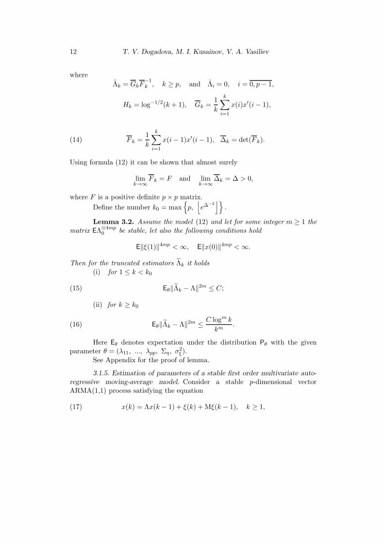
where
Λk = GkF−1k , k ≥ p, and Λi = 0, i = 0, p− 1,
Hk = log−1/2(k + 1), Gk =1
k
k∑
i=1
x(i)x′(i− 1),
(14) F k =1
k
k∑
i=1
x(i− 1)x′(i− 1), ∆k = det(F k).
Using formula (12) it can be shown that almost surely
limk→∞
F k = F and limk→∞
∆k = ∆ > 0,
where F is a positive definite p× p matrix.
Define the number k0 = maxp,
⌊e∆
−2⌋
.
Lemma 3.2. Assume the model (12) and let for some integer m ≥ 1 thematrix EΛ⊗4mp
0 be stable, let also the following conditions hold
E‖ξ(1)‖4mp < ∞, E‖x(0)‖4mp < ∞.
Then for the truncated estimators Λk it holds
(i) for 1 ≤ k < k0
(15) Eθ‖Λk − Λ‖2m ≤ C;
(ii) for k ≥ k0
(16) Eθ‖Λk − Λ‖2m ≤ C logm k
km.
Here Eθ denotes expectation under the distribution Pθ with the givenparameter θ = (λ11, ..., λpp, Ση, σ2
ξ ).
See Appendix for the proof of lemma.
3.1.5. Estimation of parameters of a stable first order multivariate auto-regressive moving-average model. Consider a stable p-dimensional vectorARMA(1,1) process satisfying the equation
(17) x(k) = Λx(k − 1) + ξ(k) +Mξ(k − 1), k ≥ 1,

Truncated estimation method and applications 13
where Λ and M are p × p stable matrices. We assume the parameter Λ to beunknown and M to be known. The random vectors ξ(k) for k ≥ 1 are i.i.d. withzero mean and finite variance σ2 = E‖ξ(1)‖2.
Let the truncated estimators of the autoregressive parameter Λ be basedon the following Yule-Walker type estimators
Λk = ΦkG−1k , k ≥ 2, Λ0 = Λ1 = 0,
where
Φk =1
k − 1
k∑
i=2
x(i)x′(i− 2), Gk =1
k − 1
k∑
i=2
x(i− 1)x′(i− 2),
and have the form
(18) Λk = Λkχ(|∆k| ≥ Hk
), k ≥ 2.
Here ∆k = det(Gk) and Hk = log−1/2 k. It can be shown that the limit (in almostsure sense) ∆ = lim
k→∞∆k is nonzero if the matrix G defined as
G = ΛF +MΣ, F =∑
n≥0
ΛnΣ(Λ′)n,
(19) Σ = ΛΣM′ +MΣΛ′ +Σ+MΣM′, Σ = Eξ(1)ξ′(1)
is non-singular.
Define the number k0 = maxp,
⌊e∆
−2⌋
.
Lemma 3.3. Assume the model (17) and let for some integer m ≥ 1 theconditions
E‖ξ(1)‖4pm < ∞, E‖x(0)‖4pm < ∞be true. Assume also that the matrix G is non-singular. Then the truncatedestimators Λk satisfy
(i) for 1 ≤ k < k0
(20) Eθ‖Λk − Λ‖2m ≤ C;
(ii) for k ≥ k0
(21) Eθ‖Λk − Λ‖2m ≤ C logm k
km.
14 T. V. Dogadova, M. I. Kusainov, V. A. Vasiliev
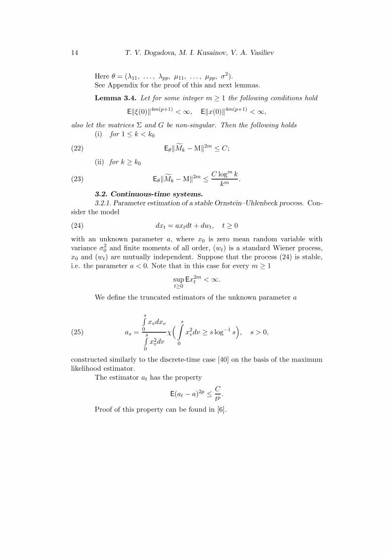
Here θ = (λ11, . . . , λpp, µ11, . . . , µpp, σ2).See Appendix for the proof of this and next lemmas.
Lemma 3.4. Let for some integer m ≥ 1 the following conditions hold
E‖ξ(0)‖4m(p+1) < ∞, E‖x(0)‖4m(p+1) < ∞,
also let the matrices Σ and G be non-singular. Then the following holds(i) for 1 ≤ k < k0
(22) Eθ‖Mk −M‖2m ≤ C;
(ii) for k ≥ k0
(23) Eθ‖Mk −M‖2m ≤ C logm k
km.
3.2. Continuous-time systems.
3.2.1. Parameter estimation of a stable Ornstein–Uhlenbeck process. Con-sider the model
(24) dxt = axtdt+ dwt, t ≥ 0
with an unknown parameter a, where x0 is zero mean random variable withvariance σ2
0 and finite moments of all order, (wt) is a standard Wiener process,x0 and (wt) are mutually independent. Suppose that the process (24) is stable,i.e. the parameter a < 0. Note that in this case for every m ≥ 1
supt≥0
Ex2mt < ∞.
We define the truncated estimators of the unknown parameter a
(25) as =
s∫0
xvdxv
s∫0
x2vdv
χ( s∫
0
x2vdv ≥ s log−1 s), s > 0,
constructed similarly to the discrete-time case [40] on the basis of the maximumlikelihood estimator.
The estimator at has the property
E(at − a)2p ≤ C
tp.
Proof of this property can be found in [6].
Truncated estimation method and applications 15
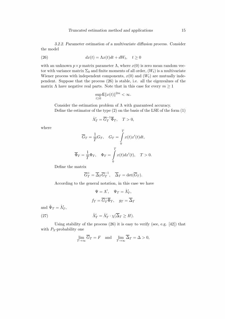
3.2.2. Parameter estimation of a multivariate diffusion process. Considerthe model
(26) dx(t) = Λx(t)dt+ dWt, t ≥ 0
with an unknown p×p matrix parameter Λ, where x(0) is zero mean random vec-tor with variance matrix Σ0 and finite moments of all order, (Wt) is a multivariateWiener process with independent components, x(0) and (Wt) are mutually inde-pendent. Suppose that the process (26) is stable, i.e. all the eigenvalues of thematrix Λ have negative real parts. Note that in this case for every m ≥ 1
supt≥0
E‖x(t)‖2m < ∞.
Consider the estimation problem of Λ with guaranteed accuracy.Define the estimator of the type (2) on the basis of the LSE of the form (1)
Λ′T = G
−1T ΦT , T > 0,
where
GT =1
TGT , GT =
T∫
0
x(t)x′(t)dt,
ΦT =1
TΦT , ΦT =
T∫
0
x(t)dx′(t), T > 0.
Define the matrix
G+T = ∆TG
−1T , ∆T = det(GT ).
According to the general notation, in this case we have
Ψ = Λ′, ΨT = Λ′T ,
fT = G+TΦT , gT = ∆T
and ΨT = Λ′T ,
(27) Λ′T = Λ′
T · χ(∆T ≥ H).
Using stability of the process (26) it is easy to verify (see, e.g. [42]) thatwith PΛ-probability one
limT→∞
GT = F and limT→∞
∆T = ∆ > 0,

16 T. V. Dogadova, M. I. Kusainov, V. A. Vasiliev
where F is a positive definite p× p matrix.
Then
f = Λ′∆, g = ∆.
We show in Appendix that there exists a given number CΛ such that forevery T > 0
(28) supΛ∈Λ0
EΛ‖ΛT − Λ‖2 ≤ CΛ
T,
where Λ0 is a compact set from the stable region of the process (x(n)).
3.2.3. Parameter estimation of one-parameter delay differential equation.Assume w = wt, t ≥ 0 is a real-valued standard Wiener process, b is a real numberand x = (xt, t ≥ −r) is a solution of the stochastic delay differential equation
(29) dxt = bxt−r + dwt, t ≥ 0
with some fixed initial condition xt = X0(t), t ∈ [−r, 0], where X0(·) is a cadlagstochastic process independent of w(·). Note that the process (29) is stable whenthe parameter b ∈ (−π/2r, 0), see [10].
The solution x of (29) exists, it is pathwise uniquely determined and canbe represented as (see, e.g., [10, 31])
xt = x0(t)X0(0) + b
0∫
−r
x0(t− s− r)X0(s)ds +
t∫
0
x0(t− s)dws, t ≥ 0.
Obviously, it has continuous paths for t ≥ 0 with probability one and,conditionally on X0(·), x is a Gaussian zero mean process. Here x0(t), t ≥ −rdenotes the so-called fundamental solution of the deterministic equation
x0(t) = bx0(t− r), x0(0) = 1 and x0(t) = 0, t ∈ [−r, 0).
The truncated estimator of the unknown parameter b can be defined onthe basis of the MLE as follows
(30) bt =
t∫rxv−rdxv
t∫rx2v−rdv
χ
t∫
r
x2v−rdv ≥ t log−1 t
, t > r.
Truncated estimation method and applications 17
Define the number σ20 =
∞∫
0
x20(v)dv.
Estimators (30) have the properties (see Appendix)
(31) E(bt − b)2m ≤ C log2m t
tm, m ≥ 1.
Estimation problems for stochastic differential equations with time delayhave been considered using asymptotic and sequential approaches in a few papersup until now – see, e.g., [10, 17, 18] and the references therein.
3.2.4. Parameter estimation of a stable non-Gaussian Ornstein–Uhlenbeckprocess by discrete-time observations. The results presented below allow statis-tical inferences for continuous-time stochastic systems by finite sample size ofobservations. Moreover, one of the main assumptions is a discrete scheme of ob-servations. It corresponds to numerous real situations, in particular in problemsof financial mathematics.
Consider the following regression model
(32) dx(t) = ax(t)dt+ dξ(t), 0 ≤ t ≤ T
with an initial condition x(0) = x0 having finite moments of all order. Hereξ(t) = ρ1W (t) + ρ2Z(t), ρ1 6= 0 and ρ2 are some constants, (W (t), t ≥ 0) is astandard Wiener process on a probability space (Ω, F , Ftt≥0, P ), adapted
to a filtration Ftt≥0, Z(t) =
Nt∑
k=1
Yk, where Yk, k ≥ 1 are i.i.d.r.v.’s with finite
moments of all order and (Nt) is a Poisson process with the intensity λ > 0.It should be noted that for ρ2 = 0 the process (32) is an Ornstein–
Uhlenbeck process.We assume that the unknown parameter lies within the interval a ∈
[−∆,−δ], where δ and ∆ > δ are known positive numbers.The problem is to estimate the parameter a by observations of the discrete-
time process y = (yk)
yk = x(tk), tk =k
nT, k = 0, n.
Using the representation for the solution of the equation (32) we get therecurrent equation for the observations (yk):
(33) yk = byk−1 + ηk, k = 1, n,

18 T. V. Dogadova, M. I. Kusainov, V. A. Vasiliev
where b = eaT/n, ηk =
tk∫
tk−1
ea(tk−s)dξ(s) are i.i.d.r.v.’s with
Eaηk = 0, σ2 := Daηk =1
2a(ρ21 + λρ22)[b
2 − 1].
Moreover, for this model all the moments σ2m = Eaη2mk are finite and
there exist their upper bounds σ2m = supa≤−δ
σ2m, m ≥ 1.
Define the estimator an of a with a guaranteed accuracy using an estima-tor bn of b as follows
(34) an =n
Tlog bn, n ≥ 1,
where the estimator bn is constructed on the basis of the LSE bn, obtained usingthe equation (33)
bn = bn · χ(gn ≥ H) + Lχ(gn < H), bn =fngn
.
Here L = [e−δT/n + e−∆T/n]/2,
fn =1
n
n∑
k=1
ykyk−1, gn =1
n
n∑
k=1
y2k−1
and the number g is defined as
g =σ2
1− b2.
Then the estimator bn has all the properties of the estimator λN , definedin (4). In particular, according to Theorem 2.1, which holds for this model forall m ≥ 1 and µ ≥ 1, the following inequalities
(35) supa≤−δ
Ea(bn − b)2m ≤ C(m)
nm+
C(µ)
nµ, n ≥ 1
for an arbitrary 0 < H ≤ σ2 hold, where
σ2 =1
2δ(21 + λ22)[1− r2], r = e−δ

Truncated estimation method and applications 19
and numbers C(m), C(µ) are known.Using (34) and (35) it is easy to verify the following property of estimators
an for every m ≥ 1 and µ > m :
supa∈[−∆,−δ]
Ea(an − a)2m ≤ (nT−1e∆T/n)2mC(m)
nm+
C(µ)
nµ
, n ≥ 1.
Proofs of results of this section can be found in [40].
4. Optimal adaptive prediction.
4.1. Discrete-time systems.
4.1.1. Optimal adaptive prediction of VAR(1). Consider the problem ofoptimal adaptive one-step prediction for the vector process (9). It is well knownthat the optimal in the mean square sense one-step predictor is the conditionalexpectation of the process with respect to its past, i.e.
xopt(k) = Λx(k − 1), k ≥ 1.
Substituting Λ with its estimator Λk defined in (10) one obtains the one-steppredictors of the form
x(k) = Λk−1x(k − 1), k ≥ 1,
for which the corresponding prediction errors have the following form
e(k) = x(k)− x(k) = (Λ− Λk−1)x(k − 1) + ξ(k).
Let e2(n) denote the sample mean of squared prediction error
e2(n) =1
n
n∑
k=1
‖e(k)‖2.
Define the loss function
Ln =A
ne2(n) + n,
where the parameter A(> 0) is the cost of prediction error. Such a loss functionformulates the problem of choosing between empirical mean-squared predictionaccuracy versus costs of increasing the sample size. Define the risk function
Rn = EθLn =A
nEθe
2(n) + n.

20 T. V. Dogadova, M. I. Kusainov, V. A. Vasiliev
Here θ = (λ11, . . . , λpp, σ2), where σ2 = E‖ξ(1)‖2.
Using the property (11) it can be shown that
Rn ≈ A
nσ2 + n
if E‖ξ(1)‖8p < ∞, E‖x(0)‖8p < ∞. Minimization of this expression by n yieldsthe optimal sample size of the form
(36) noA = A1/2σ
and the corresponding approximate minimal risk value
RnoA≈ 2A1/2σ,
where σ :=√σ2.
The requirements can be further refined to E‖ξ(1)‖4p < ∞, E‖x(0)‖4p <∞ by using projB Λk instead of Λk, where B is a closed ball that contains thestability region of the matrix parameter Λ.
However the expression for noA is of little practical use as it contains the
unknown parameter σ. For this reason one replaces optimal sample size noA with
an estimate of the following form
(37) TA = infn≥nA
n ≥ A1/2σn
,
where nA is the initial sample size depending on A and specified below,
σ2n =
1
n
n∑
k=1
‖x(k) − Λnx(k − 1)‖2.
The modified risk takes the form
RA = EθLTA= AEθ
1
TAe2(TA) + EθTA.
Theorem 4.1. Let E‖ξ(1)‖8p+4 < ∞, E‖x(0)‖8p+4 < ∞ and nA in (37)be such that
nA = o(A1/2) as A → ∞, nA ≥ maxk0, Ar log2 A, r ∈ [2/5, 1/2).
Then the following holds
TA
noA
−−−−→A→∞
1 Pθ-a.s.,EθTA
noA
−−−−→A→∞
1,RA
RnoA
−−−−→A→∞
1.
Truncated estimation method and applications 21
For proof of Theorem 4.1 see Section 4.2 in [22].Assertions of Theorem 4.1 establish the asymptotic equivalence of TA and
noA, as well as of RA and Rno
A.
Remark 3. Note that similar result holds for the scalar first-order au-toregression under lower restrictions to the model’s parameters (see Remark 2).
Since in Section 3.2.3 the observed process satisfies the scalar equation offirst-order autoregression then similar result on adaptive optimal prediction canbe obtained by using the estimators presented in Sections 3.1.1 and 3.1.3.
4.1.2. Optimal adaptive prediction of VRCA(1). Consider the problemof optimal adaptive one-step prediction for the VRCA(1) process (12). The pre-dictions and prediction errors are defined as follows
x(k) = Λk−1x(k − 1), k ≥ 1,
where Λk is defined in (13),
e(k) = x(k)− x(k) = (Λ− Λk−1)x(k − 1) + η(k − 1)x(k − 1) + ξ(k),
e2(n) =1
n
n∑
k=1
‖e(k)‖2.
The loss and risk functions are
Ln =A
ne2(n) + n, Rn =
A
nEθe
2(n) + n.
Using the property (16) it can be shown that if E‖ξ(1)‖8p < ∞,E‖x(0)‖8p < ∞ and the matrix EΛ⊗8p
0 is stable then
Rn ≈ A
nσ2 + n,
whereσ2 = σ2
ξ + tr(ΣηF ).
The optimal sample size then has the form analogous to that of (36)
noA = A1/2σ.
Define the stopping time
(38) TA = infn≥nA
n ≥ A1/2σn
,
22 T. V. Dogadova, M. I. Kusainov, V. A. Vasiliev
where nA is some function of A defined below and
σ2n =
1
n
n∑
k=1
‖x(k) − Λnx(k − 1)‖2.
Denote
RA = EθLTA= AEθ
1
TAe2(TA) + EθTA.
Theorem 4.2. Let E‖ξ(1)‖8p+4 < ∞, E‖x(0)‖8p+4 < ∞. Let also nA in(38) be such that
nA = o(A1/2) as A → ∞, nA ≥ maxk0, Ar log2 A, r ∈ [2/5, 1/2).
Then the following holds
(39)TA
noA
−−−−→A→∞
1 Pθ-a.s.,EθTA
noA
−−−−→A→∞
1,RA
RnoA
−−−−→A→∞
1
for every θ ∈ Θ8p+4, where Θm = θ : EΛ⊗m0 is stable, 0 < σ2
ξ , σ2η < ∞.
See Appendix for the proof of theorem.
4.1.3. Optimal adaptive prediction of VARMA(1). Consider the problemof optimal adaptive one-step prediction for the VARMA(1,1) process (17). As-sume that the matrix parameter M is known. Then the predictions and predictionerrors are defined as follows
x(k) = Λk−1x(k − 1) +Mξ(k − 1), k ≥ 1,
e(k) = x(k)− x(k) = (Λ− Λk−1)x(k − 1) +M(ξ(k − 1)− ξ(k − 1)) + ξ(k),
where the estimators Λk were defined in (18) and
ξ(k) =k−1∑
i=0
(−M)i(x(k − i)− Λkx(k − 1− i)
).
Define the loss and risk functions
Ln =A
ne2(n) + n, e2(n) =
1
n
n∑
k=1
‖e(k)‖2,
Rn =A
nEθe
2(n) + n.

Truncated estimation method and applications 23
Analogously to the previous subsections, if E‖ξ(0)‖8p < ∞, E‖x(0)‖8p <∞, then it can be shown that
Rn ≈ A
nσ2 + n
and the optimal sample size is
noA = A1/2σ.
The corresponding approximate minimal risk value is
RnoA≈ 2A1/2σ.
If σ is unknown one defines the stopping time of the form
(40) TA = infn≥nA
n ≥ A1/2σn
,
where nA is a function of A defined later, and the estimator of the parameter σ2
is defined as follows
σ2n = Jp
1
n
n∑
k=1
(I +M⊗2)−1 × vec[(x(k)− Λnx(k − 1)
)(x(k)− Λnx(k − 1)
)′],
where
Jp = 〈ji〉1×p2 , ji =1, i = 1 + (l − 1)(p + 1) for l = 1, p; 0 otherwise.
Here 〈ji〉1×p2 denotes a row vector of the length p2 with elements ji.Define
RA = AEθ1
TAe2(TA) + EθTA.
Theorem 4.3. Let E‖ξ(1)‖8p+4 < ∞, E‖x(0)‖8p+4 < ∞. Let also nA in(40) be such that
nA = o(A1/2) as A → ∞, nA ≥ maxk0, Ar log2 A, r ∈ [2/5, 1/2).
Then the following holds
TA
noA
−−−−→A→∞
1 Pθ-a.s.,EθTA
noA
−−−−→A→∞
1,RA
RnoA
−−−−→A→∞
1.
Proof of Theorem 4.3 is analogous to that of Theorem 4.1. See also [20],where Theorem 4.3 is proved in a more specific case of uncorrelated and identicallydistributed components ξj(k), j = 1, p of noises ξ(k). This condition allows oneto use a simpler form of the estimators σ2
n and apart from that difference theproofs are identical.

24 T. V. Dogadova, M. I. Kusainov, V. A. Vasiliev
4.2. Continuous-time systems.
4.2.1. Prediction of the Ornstein–Uhlenbeck process. Consider the model(24). The problem is to construct a predictor for xt by observations xt−u =(xs)0≤s≤t−u which is optimal in the sense of the risk function introduced below.Here u > 0 is a fixed time delay.
Using the solution of (24) we obtain the following representation
(41) xt = λxt−u + ξt,t−u, t ≥ u,
where ξt,t−u =
t∫
t−u
ea(t−s)dws, λ = eau. Applying properties of the Ito integral it
is easy to make sure that
Eξt,t−u = 0, σ2 := Eξ2t,t−u =1
2a[λ2 − 1].
Optimal in the mean square sense predictor x0t for xt is the conditionalmathematical expectation of xt under the condition of xt−u which can be foundby (41)
x0t = λxt−u, t ≥ u.
Since the parameters a and λ are unknown, we define the adaptive pre-dictor
(42) xt = λt−uxt−u, t ≥ u,
where λs = easu, as = proj(−∞,0]as, estimator as is defined in (25).
Define the prediction errors of x0t and xt as
e0t = xt − x0t = ξt,t−u,
et = xt − xt = (λ− λt−u)xt−u + ξt,t−u, t ≥ u.
Now we define the loss function
Lt =A
te2(t) + t, t ≥ u,
where e2(t) =1
t
∫ t
ue2sds and the parameter A > 0 is the cost of prediction error.
We also define the risk function Rt = ELt which has the following form
Rt =A
tEe2(t) + t

Truncated estimation method and applications 25
and consider optimization problem
Rt → mint
.
For the optimal predictors x0t it is possible to optimize the correspondingrisk function
(43) R0t = E
(A
t(e0(t))2 + t
)=
Aσ2
t+ t → min
t,
where (e0(t))2 =1
t
t∫
u
(e0s)2ds.
In this case the optimal duration of observations T 0A and the corresponding
value of R0t are respectively
(44) T 0A = A
1
2σ, R0T 0A= 2A
1
2σ,
where σ :=√σ2.
However, since a and consequently σ are unknown and both T 0A and R0
T 0A
depend on a, the optimal predictor can not be used. Then we define the estimatorTA of the optimal time T 0
A as
(45) TA = inft ≥ tA : t ≥ A1/2σtA,
where tA := A1/2 ·log−1A = o(A1/2). Here σt :=√
σ2t is the estimator of unknown
σ, where
(46) σ2t =
1
2θt · [λ2
t − 1]
and θt is the truncated estimator of θ = a−1 defined as follows
θt = a−1t · χ[at ≤ − log−1 t], t > 0.
Estimators at, λt and σt, which are used in adaptive predictors, have theproperties given in Lemma 4.1 below which will be proved in Appendix.
Lemma 4.1. Assume the model (24). Then the estimators at, λt andσt are strongly consistent. Moreover, for t− u > s0 := exp(2|a|) the followingproperties hold
(47) E(at − a)2p ≤ C
tp

26 T. V. Dogadova, M. I. Kusainov, V. A. Vasiliev
and
(48) E(λt − λ)2p ≤ C
tp, p ≥ 1,
(49) E(σ2t − σ2)2p ≤ C log2p t
tp, p ≥ 1.
Analogously to [22, 39] and [38], our purpose is to prove the asymptoticequivalence of TA and T 0
A in the almost surely and mean senses and the optimalityof the presented adaptive prediction procedure in the sense of equivalence of R0
A
and the obviously modified risk
(50) RA = A · E 1
TAe2(TA) + ETA.
Theorem 4.4. Assume the model (24) and tA that is defined in (45).Let the predictors xt be defined by (42), the times T 0
A, TA and the risk functionsR0
t , RA defined by (44), (45) and (43), (50) respectively. Then for every a < 0
TA
T 0A
−−−−→A→∞
1 Pθ-a.s.,ETA
T 0A
−−−−→A→∞
1,RA
R0A
−−−−→A→∞
1.
Proof of Theorem 4.4 can be found in [7].
4.2.2. Prediction of the multivariate diffusion process. Consider the model(26). The problem is to construct a predictor for x(t) defined in (26) by obser-vations xt−u = (x(s))0≤s≤t−u which is optimal in the sense of the risk functionintroduced below. Here u > 0 is a fixed time delay.
Using the solution of (26) we obtain the following representation
(51) x(t) = Bx(t− u) + ξt,t−u, t ≥ u,
where ξt,t−u =
t∫
t−u
eΛ(t−s)dWs, B = eΛu. Applying properties of the Ito integral
it is easy to verify that
Eξt,t−u = 0, σ2 := E‖ξt,t−u‖2 =u∫
0
‖eΛs‖2ds.
Truncated estimation method and applications 27
Optimal in the mean square sense predictor x0(t) for x(t) is the conditionalmathematical expectation of x(t) under the condition of xt−u which can be foundusing (51)
x0(t) = Bx(t− u), t ≥ u.
Since the parameters Λ and B are unknown, we define the adaptive pre-dictor
(52) x(t) = Bt−ux(t− u), t ≥ u,
where Bt−u is the estimator of B defined as follows
Bt = eΛtu,
where Λt = projΛ0Λt, Λ0 is a compact set from the stability region of the process
(26), Λt is defined in (27).Denote the prediction errors of x0t and xt as
e0(t) = x(t)− x0(t) = ξt,t−u,
e(t) = x(t)− x(t) = (B −Bt−u)x(t− u) + ξt,t−u, t ≥ u.
Now we define the loss function
Lt =A
te2(t) + t, t ≥ u,
where
e2(t) =1
t
∫ t
u‖e(s)‖2ds
and the parameter A > 0 is the cost of prediction error.We also define the risk function Rt = ELt which has the following form
Rt =A
tEe2(t) + t
and consider optimization problem
Rt → mint
.
For the optimal predictors x0(t) it is possible to optimize the correspond-ing risk function
(53) R0t = E
(A
t(e0(t))2 + t
)=
Aσ2
t+ t → min
t,

28 T. V. Dogadova, M. I. Kusainov, V. A. Vasiliev
where (e0(t))2 =1
t
t∫
u
(e0s)2ds.
In this case the optimal duration of observations T 0A and the corresponding
value of R0t are respectively
(54) T 0A = A
1
2σ, R0T 0A= 2A
1
2σ,
where σ :=√σ2.
However, since Λ and consequently σ are unknown and both T 0A and R0
T 0A
depend on a, the optimal predictor can not be used in practice. We define theestimator TA of the optimal time T 0
A as
(55) TA = inft ≥ tA : t ≥ A1/2σtA,
where tA := A1/2 ·log−1A = o(A1/2). Here σt :=√
σ2t is the estimator of unknown
σ2, where
σ2t =
u∫
0
‖eΛts‖2ds.
Estimators Λt, Bt and σt that are used in the adaptive predictors havethe properties given in Lemma 4.2 below which will be proved in Appendix.
Lemma 4.2. Assume the model (26). Then the estimators Λt, Bt andσt are strongly consistent. Moreover, for t large enough the following propertieshold
(56) E‖Λt − Λ‖2p ≤ C
tp
and
(57) E‖Bt −B‖2p ≤ C
tp, p ≥ 1,
(58) E(σ2t − σ2)2p ≤ C log2p t
tp, p ≥ 1.
Analogously to [22, 38, 39], our aim is to prove the asymptotic equivalenceof TA and T 0
A in the almost surely and mean senses and the optimality of the
Truncated estimation method and applications 29
presented adaptive prediction procedure in the sense of equivalence of R0A and
the obviously modified risk
(59) RA = A · E 1
TAe2(TA) + ETA.
Theorem 4.5. Assume the model (26) and tA that is defined in (55).Let the predictors xt be defined by (52), the times T 0
A, TA and the risk functionsR0
t , RA defined by (54), (55) and (53), (59) respectively. Then as for every a < 0
TA
T 0A
−−−→A→∞
1 Pθ-a.s.,ETA
T 0A
−−−→A→∞
1,RA
R0A
−−−→A→∞
1.
The proof of Theorem 4.5 is similar to that of Theorem 4.4.
4.2.3. One-parameter delay differential equation. Consider the model(29). We construct optimal and adaptive predictors for the process (29). Optimalin the mean square sense predictor is the conditional mathematical expectation
z(k)t (t− u) = E(xt|xt−u),
which satisfies the following equation
(60)
z(k)t (t− u) = xt−u + b
t−(u−r)∧t∫
t−u
xv−rdv + b
t∫
t−(u−r)∧t
z(0)v−krdv +
+ b
k−1∑
i=1
t−r∫
t
z(i)v−(k−i)rdv, kr < u ≤ (k + 1)r, t > u.
Here α ∧ β denotes the minimum between α and β.
Since the parameter b in the definition of the optimal predictors z(k)t (t−
u) is unknown, we define the adaptive predictor by formula (60) replacing theunknown b with bt−u, where bt−u is the projection
bt−u = proj[−π/2r,0]bt−u
of the truncated estimator of the parameter b which is proposed in (30).
Define the numbers σ20 =
∞∫
r
x20(v)dv and s0 = maxr, exp(σ−20 ).

30 T. V. Dogadova, M. I. Kusainov, V. A. Vasiliev
Denote the adaptive prediction error and rewrite it in the form
e(k)t (t− u) := xt − z
(k)t (t− u) = e0t + e
(k)t (t− u),
where e0t (t−u) = xt−E(xt|xt−u) and e(k)t (t−u) = z
(k)t (t−u)− z
(k)t (t−u). Then
for every fixed k ≥ 0 the following limit inequalities hold
limt→∞
t(E(e(k)t (t− u))2 − σ2
0) ≤ C.
If it is known that b ∈ [b0, b1], −π/2r < b0 < b1 < 0, then for t−u > s1 == maxr, exp(σ−2
1 ) , where σ21 = inf
b∈[b0,b1]σ20 the non-asymptotic property is ful-
filled
E(e(k)t (t− u))2 − σ2
0 ≤ C
t.
These properties mentioned in [6] can be used to prove optimality in thesense of considered above risk functions.
4.2.4. Stable non-Gaussian Ornstein–Uhlenbeck process by discrete-timeobservations. Results presented in Sections 3.2.4, 4.2.1 make it possible to solvethe prediction problem for the process defined in (32) in every point.
For some u ∈ (0, 1] define the numbers sk = (k − 1 + u)h, h = T/n. Weintroduce the process
z = (zk)k≥0, z = x(sk).
Using the representation for the solution of the equation (32) we get theequation for the observations (zk, yk)
(61) zk = bu · yk−1 + ηk,u, ηk,u =
∫ sk
tk−1
ea(sk−t)dξ(t),
bu = eauh, Eηk,u = 0, σ2u = Eη2k,u =
1
2a(ρ21 + λρ22)[b
2u − 1].
The adaptive optimal prediction problem can be solved similarly to Sec-tion 4.1.1 for predictors
zk = bu,k−1yk−1, bu,k−1 = bu,k−1 · χ[
k∑
i=1
y2i−1 ≥ k log−1 k
],
where bu,k−1 is the LSE obtained from the equation (61).
Truncated estimation method and applications 31
The risk function can be defined analogously to Section 4.1.1 with pre-diction errors
ek = zk − zk.
Properties presented in Theorem 4.1 hold for the predictors zk as well.
Appendix.
P r o o f o f L emma 3.2 is similar to that of Lemma 3.1. For this reasonbelow we present those proof parts that are essentially different between the two.See also [21] for the proof in scalar case.
For this proof we first need to establish the properties of Eθx(k)x′(k).
Solving the equation (12) yields
x(k) =
k−1∑
i=0
i∏
j=1
Λk−jξ(k − i) +
k∏
j=1
Λk−jx(0)
and thus,
(62)
Eθx(k)x′(k) = Eθ
k−1∑
i=0
i∏
j=1
Λk−jξ(k − i)ξ′(k − i)
1∏
j=i
Λ′k−j +
+ Eθ
k∏
j=1
Λk−jx(0)x′(0)
1∏
j=k
Λ′k−j,
here products∏
are ordered, i.e.
1∏
j=k
Λ′k−j = Λ′
0 · Λ′1 · . . . · Λ′
k−1 6=k∏
j=1
Λ′k−j.
To further break down the resulting expression we will use matrix vector-ization operator vec[·], which has the following property (see, e.g., [32])
(63) vec[V Y Z] = (Z ′ ⊗ V ) vec[Y ].
Applying vec[·] and its property (63) to (62), one obtains
(64)
vec[Eθx(k)x′(k)] =
k−1∑
i=0
Eθ
( i∏
j=1
Λk−j
)⊗2
vec[Σ] +
+ Eθ
( k∏
j=1
Λk−j
)⊗2
vec[Ex(0)x′(0)].

32 T. V. Dogadova, M. I. Kusainov, V. A. Vasiliev
Using the Kronecker product’s property (S ⊗ V ) · (Y ⊗ Z) = S · Y ⊗ V · Z we
have
( i∏
j=1
Λk−j
)⊗2
=i∏
j=1
Λ⊗2k−j and since η(k), k ≥ 1, are independent, then
Eθ
( i∏
j=1
Λk−j
)⊗2
=
i∏
j=1
EθΛ⊗2k−j = Λ
i,
where Λ = EΛ⊗20 . Recall that Λ is stable (see conditions in 3.1.4). This allows us
to simplify (64) in the following manner
(65)vec[Eθx(k)x
′(k)] =
k−1∑
i=0
Λivec[Σ] + Λ
kvec[Ex(0)x′(0)] =
= (I − Λ)−1(I − Λk) vec[Σ] + Λ
kvec[Ex(0)x′(0)].
Letting k → ∞ we get
(66) vec[F ] = (I − Λ)−1 vec[Σ].
Using this equality as well as (65), it can be shown that
(67)
∞∑
k=0
‖Eθx(k)x′(k)− F )‖2 ≤ C,
(68)1
n
n∑
k=1
∣∣ tr(Ψ(Eθx(k − 1)x′(k − 1)− F ))∣∣ = O(n−1), n → ∞.
Now we proceed to prove the first assertion (15) of Lemma 3.2. Denotez1(k) = vec[x(k)x′(k)], k ≥ 1. From (12) and (63) it follows that the equationfor z1(k) can be written as
z1(k) = Λ⊗2k−1z1(k − 1) + ǫ1(k),
ǫ1(k) = (ξ(k)⊗ Λk−1)x(k − 1) + (Λk−1 ⊗ ξ(k))x(k − 1) + vec[ξ(k)ξ′(k)].
Examine ‖z1(k)‖1, where ‖a‖1 =
p∑
i=1
|ai|. The condition necessary for
supk≥1
Eθ‖z1(k)‖1 < ∞ is stability of the matrix EΛ⊗20 as well as finiteness of ξ(1)
Truncated estimation method and applications 33
and x(0) (see (65)). If we then consider the process z2(k) = vec[z1(k)z′1(k)],
which satisfies the equation
z2(k) = Λ⊗4k−1z2(k − 1) + ǫ2(k),
it turns out that supk≥1
Eθ‖z2(k)‖1 < ∞, if the matrix Λ⊗40 is stable and the fourth
moments of ξ(1), x(0) are finite. Continuing in this manner and using the fol-lowing obvious inequality
supk≥1
Eθ‖x(k)‖2 ≤ supk≥1
Eθ‖ vec[x(k)x′(k)]‖1,
we find that conditions of the lemma guarantee
(69) supk≥0
Eθ‖x(k)‖4mp ≤ C, supk≥0
Eθ∆2mk ≤ C.
Using (69) one can verify the following inequality
(70) Eθ‖Λk − Λ‖2m ≤ 1
H2mk
Eθ‖ζkF+k ‖2m + ‖Λ‖2mPθ(∆k < Hk),
whereF
+k = ∆kF
−1k , k ≥ p,
ζk =1
k
k∑
i=1
η(i − 1)x(i− 1)x′(i− 1) +1
k
k∑
i=1
ξ(i)x′(i− 1).
Since x(i − 1) and η(i − 1) are mutually independent, the process (ζk)k≥1 is, infact, a sum of two martingales. Thus, analogously to (4.4) in [22], it can be shownthat Eθ‖ζk‖2mp ≤ C · k−mp. Then for k ≥ p the inequality
(71)1
H2mk
Eθ‖ζkF+k ‖2m ≤ C lnm k
km
follows from Holder’s inequality, and hence (15) holds.To tackle Eθ(∆k − ∆)2m, where ∆ = det(F ), one needs to determine
the properties of (F k − F ). We will use the following identity
(72) vec[F ] = (I − Λ⊗2)−1(vec[Σ] + η vec[F ]),
where η = Eη⊗2(0). To obtain it we use the representation (66) as follows
(I − Λ⊗2)−1(vec[Σ] + η vec[F ]) = (I − Λ⊗2)−1(vec[Σ] + η(I − Λ)−1 vec[Σ]) =
= (I − Λ⊗2)−1((I − Λ)(I − Λ)−1 + η(I − Λ)−1
)vec[Σ] =
= (I − Λ⊗2)−1(I − (Λ⊗2 + η) + η
)(I − Λ)−1 vec[Σ] = (I − Λ)−1 vec[Σ] = vec[F ].
34 T. V. Dogadova, M. I. Kusainov, V. A. Vasiliev
Using the definition (14) of F k it can be shown that
(73) F k = ΛF kΛ′ +Σ+
1
k
k∑
i=1
η(k−1)x(k−1)x′(k−1)η′(k−1) + Sk,
where
Sk =1
k(x(k)x′(k)− x(0)x′(0)) +m1,k +m2,k +m′
2,k,
m1,k =1
k
k∑
i=1
(ξ(i)ξ′(i)− Σ), m2,k =1
k
k∑
i=1
ξ(i)x′(i− 1)Λ′k−1.
Note that Sk has a martingale structure. One can show, analogously to (4.4) in[22], that
(74) Eθ‖Sk‖2m ≤ C · k−m.
Solving the equation (73) yields
F k =∑
n≥0
Λn
(Σ+
1
k
k∑
i=1
η(k−1)x(k−1)x′(k−1)η′(k−1) + Sk
)(Λ′)n.
Applying vec[·] to both sides and taking into account its properties as well as theidentity (Λn)⊗2 = (Λ⊗2)n, one gets
vec[F k] =∑
n≥0
(Λ⊗2)n vec
[Σ+
1
k
k∑
i=1
η(k−1)x(k−1)x′(k−1)η′(k−1) + Sk
]=
= (I − Λ⊗2)−1
(vec[Σ] +
1
k
k∑
i=1
η⊗2(k − 1) vec[x(k−1)x′(k−1)] + vec[Sk]
).
From this representation and (72) it follows that
(75) vec[F k − F ] = (I − Λ⊗2)−1
(1
k
k∑
i=1
(η⊗2(k−1) vec[x(k−1)x′(k−1)] −
− η Eθ vec[x(k−1)x′(k−1)])+
1
k
k∑
i=1
η vec[Eθx(k−1)x′(k−1)− F ] + vec[Sk]
).

Truncated estimation method and applications 35
The first summand inside the parentheses is a normalized martingale, for whichthe following holds, analogously to (74),
1
k2mEθ
( k∑
i=1
(η⊗2(k − 1) vec[x(k − 1)x′(k − 1)] −
− Eθη⊗2(k − 1) vec[x(k − 1)x′(k − 1)]
))2m
≤ C
km.
The second summand is non-random. From (65)-(67) we get
1
k2m
( k∑
i=1
η vec[Eθx(k−1)x′(k−1)− F ]
)2m
≤ C
km.
Then from (75) as well as (69) and (74) it follows that
(76) Eθ‖F k − F‖2m ≤ C
km.
The second assertion of Lemma 3.2 follows from (70), (71), Chebyshev’s inequalityand (76). Lemma 3.2 is proven.
P r o o f o f L emma 3.3 is similar to that of Lemma 3.1. For such k thatGk is non-singular we can write
Λk − Λ =1
∆k
ζkG+k , k ≥ 2,
where
ζk =1
k − 1
k∑
i=2
(ξ(i) +Mξ(i− 1)
)x′(i− 2), G
+k = ∆kG
−1k .
Hence
(77) Eθ‖Λk − Λ‖2m ≤ 1
H2mk
Eθ‖ζkG+k ‖2m + ‖Λ‖2mPθ(∆k < Hk).
The martingale structure of ζk allows one to prove
(78)1
H2mk
Eθ‖ζkF+k ‖2m ≤ C lnm k
km,
and this together with (77) proves (20).
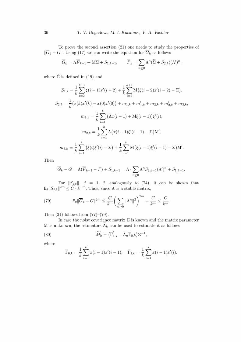
36 T. V. Dogadova, M. I. Kusainov, V. A. Vasiliev
To prove the second assertion (21) one needs to study the properties of‖Gk −G‖. Using (17) we can write the equation for Gk as follows
Gk = ΛF k−1 +MΣ+ S1,k−1, F k =∑
n≥0
Λn(Σ + S2,k)(Λ′)n,
where Σ is defined in (19) and
S1,k =1
k
k+1∑
i=2
ξ(i− 1)x′(i− 2) +1
k
k+1∑
i=2
M(ξ(i− 2)x′(i− 2)− Σ
),
S2,k =1
k
(x(k)x′(k)− x(0)x′(0)
)+m1,k +m′
1,k +m2,k +m′2,k +m3,k,
m1,k =1
k
k∑
i=1
(Λx(i− 1) +Mξ(i − 1)
)ξ′(i),
m2,k =1
k
k∑
i=1
Λ(x(i− 1)ξ′(i− 1)− Σ
)M′,
m3,k =1
k
k∑
i=1
(ξ(i)ξ′(i)− Σ
)+
1
k
k∑
i=1
M(ξ(i− 1)ξ′(i− 1)− Σ
)M′.
Then
Gk −G = Λ(F k−1 − F ) + S1,k−1 = Λ ·∑
n≥0
ΛnS2,k−1(Λ′)n + S1,k−1.
For ‖Sj,k‖, j = 1, 2, analogously to (74), it can be shown thatEθ‖Sj,k‖2m ≤ C · k−m. Thus, since Λ is a stable matrix,
(79) Eθ‖Gk −G‖2m ≤ C
km
(∑
n≥0
‖Λn‖2)2m
+C
km≤ C
km.
Then (21) follows from (77)–(79).In case the noise covariance matrix Σ is known and the matrix parameter
M is unknown, the estimators Λk can be used to estimate it as follows
(80) Mk =(Γ′1,k − ΛnΓ0,k
)Σ−1,
where
Γ0,k =1
k
k∑
i=1
x(i− 1)x′(i− 1), Γ1,k =1
k
k∑
i=1
x(i− 1)x′(i).

Truncated estimation method and applications 37
Lemma 3.3 is proven.
P r o o f o f L emma 3.4. Using the definition (80) of Mk we can writeits deviation as follows
Mk −M =
(1
k
k∑
i=1
(Λ− Λk)x(i − 1)x′(i− 1) +1
kMξ(0)x′(0) +
(81) +1
k
k∑
i=1
ξ(i)x′(i− 1) +1
k
k∑
i=2
Mξ(i− 1)x′(i− 2)Λ′ +
+1
k
k∑
i=2
Mξ(i − 1)ξ′(i− 2)M′ +M
k
k∑
i=1
(ξ(i− 1)ξ′(i− 1)− Σ
))Σ−1.
The last 4 summands in the parentheses (which we denote Sj,k, j = 1, 4) arenormalized martingales, for which the following can easily be shown Eθ‖Sj,k‖2m ≤
Ck−m. Observe also that by lemma’s conditions E
∥∥∥∥1
kMξ(0)x′(0)
∥∥∥∥2m
≤ Ck−2m.
For the first summand in (81), using Holder’s inequality and propertiesof the estimators Λk, we obtain for k ≥ k0
Eθ
∥∥∥∥1
k
k∑
i=1
(Λ− Λk)x(i − 1)x′(i− 1)
∥∥∥∥2m
≤
≤(Eθ‖Λ− Λk‖2m
p+1
p
) pp+1
·(Eθ
∥∥∥∥1
k
k∑
i=1
x(i− 1)x′(i− 1)
∥∥∥∥4m(p+1)) 1
p+1
≤ C lnm k
km,
which implies the second assertion (23) of lemma. When 1 ≤ k < k0 the property(20) ensures that the boundary in the above inequality is some constant C, hencethe first assertion (22) of lemma. Lemma 3.4 is proven.
P r o o f o f t h e p r o p e r t y (28). Consider the deviation of the estima-tor in the form
Λ′
T − Λ′
= (Λ′
T − Λ′
) · χ(gT ≥ H)− Λ′ · χ(gT < H) =
= G−1T · ζT · χ(gT ≥ H)− Λ
′ · χ(gT < H) := I1 + I2,
where ζT =1
T
∫ T
0x(t)dW
′
(t).

38 T. V. Dogadova, M. I. Kusainov, V. A. Vasiliev
We estimate the mathematical expectation using the Cauchy-Bunyakov-skii inequality and the properties of the Ito integral
E‖I1‖2p = E‖G+T · ζT ‖2p · g−2p
T · χ(gT ≥ H) ≤ H−2p · E‖G+T ‖2p · ‖ζT ‖2p ≤
≤ H−2p ·√
E‖G+T ‖4p · E‖ζT ‖4p ≤ C
T p.
Similarly to [4, 12] we get
E‖I2‖2p = ‖Λ‖2p ·P (gT < H) ≤ ‖Λ‖2p ·P (|gT −g| > g−H) ≤ C ·E(gT −g)2p ≤ C
T p.
Thus the property (28) is proven.
P r o o f o f t h e p r o p e r t y (31). Denote
bt − b =
t∫
r
xsdws
/ t∫
r
x2sds
· χ
t∫
r
x2sds ≥ t log−1 t
−
−b · χ
t∫
r
x2sds < t log−1 t
:= I1 + I2.
It is obvious that
E(bs − b)2m = EI2m1 + EI2m2 .
Consider each summand separately. Using Burckholder’s (see, e.g. [2])and Holder’s inequalities, we obtain
EI2m1 ≤ log2m t
t2mE
t∫
r
xsdws
2m
≤ log2m t
t2mE
t∫
r
x2sds
m
≤ Clog2m t
tm.
For the second term, by Chebyshev’s inequality and for t > max(r, exp(σ20)
m2 ) we

Truncated estimation method and applications 39
obtain
EI2m2 ≤ b2mP
1
t
t∫
r
x2sds < log−1 t
2m
=
= b2mP
σ2
0 −1
t
t∫
r
x2sds > σ20 − log−1 t
2m
≤
≤ b2m
(σ20 − log−1 t)2m
E
1
t
t∫
r
x2sds− σ20
2m
≤ C
tm.
The last inequality follows from formulae (5.9)–(5.11) in [19]. The prop-erty (31) is proven.
P r o o f o f Th e o r em 4.2 is similar to that of Theorem 4.1. Below arethose proof parts that are essentially different between the two. See also [21] forthe proof in scalar case.
From the conditions it follows that for θ ∈ Θ8p+4
supk≥0
Eθ‖x(k)‖8p+4 ≤ C.
We now prove the first assertion in (39). Rewrite the estimators σ2n in the
following form
σ2n =
1
n
n∑
k=1
(‖ξ(k)‖2 + ‖η(k − 1)x(k − 1)‖2) +Wn + νn,
where
Wn =1
n
n∑
k=1
‖(Λn − Λ)x(k − 1)‖2, νn =2
n
n∑
k=1
ξ′(k)η(k − 1)x(k − 1)−
− 2
n
n∑
k=1
(ξ′(k) + x′(k − 1)η′(k − 1))(Λn − Λ)x(k − 1).
Next we show that
(82) σ2n −−−→
n→∞σ2
Pθ-a.s.

40 T. V. Dogadova, M. I. Kusainov, V. A. Vasiliev
Using Chebyshev’s inequality and (16) we have for some 0 < β ≤ 4+2p−1
and every ǫ > 0
Pθ(‖Λn − Λ‖ ≥ ǫ) ≤ 1
ǫ2+βEθ‖Λn − Λ‖2+β ≤ C ln1+
β2 n · n−(1+β
2).
Therefore, the Borel-Cantelli lemma guarantees that the estimators Λn are strongly
consistent. Together with (76) this yields the convergence WnPθ-a.s.−−−−→n→∞
0. Analo-
gously it can be shown that νnPθ-a.s.−−−−→n→∞
0.
At the same time, from Kolmogorov’s strong law of large numbers, (67)and the Borel-Cantelli lemma it follows that
1
n
n∑
k=1
(‖ξ(k)‖2 + ‖η(k − 1)x(k − 1)‖2) −−−→n→∞
σ2Pθ-a.s.
From this and from the convergencies of Wn and νn we have (82). Since, by
definition (38), TAPθ-a.s.−−−−→A→∞
∞, and thus σ2TA
Pθ-a.s.−−−−→A→∞
σ2, then
TA
A1/2σ−−−−→A→∞
1 Pθ-a.s.,
the first assertion of the Theorem is proved.The second and third assertions in (39) are proved analogously to those
of Theorem 4.1 with mn therein (see page 222 in [22]) having a different form,namely
mn =1
n
n∑
k=1
(‖ξ‖2 − σ2ξ ) +
1
n
n∑
k=1
tr(η′(k − 1)η(k − 1)x(k − 1)x′(k − 1)−
−Eθη(k−1)η′(k−1)x(k−1)x′(k−1)) +1
n
n∑
k=1
tr(Ψ(Eθx(k−1)x′(k−1)− F )
),
which is a sum of two normalized martingales and a non-random function of n,decaying as O(n−1) (see (68)). The martingale nature of mn is what makes thetwo proofs analogous. Theorem 4.2 is proven.
P r o o f o f L emma 4.1. Properties (47),(48) are proved in [6].Now we prove the assertion (49). To this end we consider the deviation
of the estimator (46)
|σ2t − σ2| =
∣∣∣∣1
2θt · [λ2
t − 1]− 1
2θ[λ2 − 1]
∣∣∣∣ =∣∣∣∣1
2[θt − θ] · [λ2
t − 1] +

Truncated estimation method and applications 41
+1
2θ[λ2
t − 1]− 1
2θ[λ2 − 1]
∣∣∣∣ ≤1
2|θt − θ|+ 1
2|θ‖λ2
t − λ2| ≤ 1
2|θt − θ|+ |θ‖λt − λ| ≤
≤∣∣∣∣1
at+
1
a
∣∣∣∣ · χ[at ≤ − log−1 t] +1
|a| · χ[at > − log−1 t] + |θ‖λt − λ| = I1 + I2 + I3.
Considering each summand separately we obtain
|I1| =∣∣∣∣a− atata
∣∣∣∣ · χ[at ≤ − log−1 t] ≤ log t
|a| |a− at|.
Whence by property (47)
EI2p1 ≤ C log2p tE|a− at|2p ≤ Clog2p t
tp.
By Chebyshev’s inequality, we get
EI2p2 ≤ C · P (at > − log−1 t) ≤ C · P (at − a > − log−1 t− a) ≤
≤ C · P (|at − a| > |a| − log−1 t) ≤ C · 1
(|a| − log−1 t)2pE(at − a)2p ≤ C · log
2p t
tp.
To finish the prove of Lemma 4.1 it is enough to apply (48) for estimation ofEI2p3 .
P r o o f o f L emma 4.2. The property (56) is proved above. Let usprove (57). Estimate the norm
‖Bt −B‖ = ‖eΛtu − eΛu‖ ≤ ‖eΛu‖ · ‖e(Λt−Λ)u − I‖ =
= ‖eΛu‖ · ‖∞∑
k=1
uk
k!(Λt − Λ)k‖ ≤ ‖eΛu‖ ·
∞∑
k=1
uk‖Λt − Λ‖kk!
=
= ‖eΛu‖ · u · ‖Λt − Λ‖ ·∑
k≥1
uk−1‖Λt − Λ‖k−1
(k − 1)! · k ≤
≤ ‖eΛu‖ · u · ‖Λt − Λ‖ · eu‖Λt−Λ‖ ≤ C · ‖Λt − Λ‖.
Then the mathematical expectation
E‖Bt −B‖2p ≤ C · E‖Λt − Λ‖2p ≤ C
tp.

42 T. V. Dogadova, M. I. Kusainov, V. A. Vasiliev
We prove now the property (58). The deviation of the estimator has the form
σ2t − σ2 =
∫ u
0
[‖eΛts‖2 − ‖eΛs‖2
]ds.
Consider the integrand
‖eΛts‖2 − ‖eΛs‖2 = tr[e(Λt+Λ
′
t)s − e(Λ+Λ′
)s]
= tre(Λ+Λ
′
)s ·[e(Λt−Λ)s+(Λ
′
t−Λ′
)s − I]
.
Using the trace property tr(AB) ≤ ‖A‖ · ‖B‖ and by the definition of the matrixexponent, we obtain
‖|eΛts‖2 − ‖eΛs‖2| ≤ ‖e(Λ+Λ′
)s‖ · ‖e(Λt−Λ)s+(Λ′
t−Λ′
)s − I‖ ≤
≤ ‖e(Λ+Λ′
)s‖ · ‖∞∑
k=1
1
k!
[(Λt − Λ) + (Λ
′
t − Λ′
)]k
sk‖ ≤
≤ ‖e(Λ+Λ′
)s‖ ·∞∑
k=1
1
k!sk · ‖(Λt − Λ) + (Λ
′ − Λ′
)‖k ≤
≤ ‖e(Λ+Λ′
)s‖ · 2 · s · ‖Λt − Λ‖ ·∞∑
k=1
sk−1 · 2k(k − 1)!
· ‖(Λt − Λ‖k−1 ≤
≤ 4s · e2‖Λ‖s · ‖Λt − Λ‖ · e‖Λt−Λ‖ ≤ C · ‖Λt − Λ‖.The last inequality uses boundedness of Λt. Thus, we obtain
E(σ2t − σ2)2p ≤ C · E‖Λt − Λ‖2p ≤ C
tp.
Lemma 4.2 is proven.
Acknowledgment. The work I. of T. V. Dogadova, M. I. Kusainovand V. A. Vasiliev, as well as 3.1.3, 4.1.1 of M. I. Kusainov and V. A. Vasiliev,and 3.1.4, 3.1.5, 4.1.2, 4.1.3 of M. I. Kusainov is supported by The Ministry of Ed-ucation and Science of the Russian Federation, Goszadanie No 2.3208.2017/4.6,also II, 3.1.1, 3.1.2, 3.2.4 of V. A. Vasiliev, 3.2.2, 3.2.3, 4.2 of T. V. Dogadovaand V. A. Vasiliev is supported by the Russian Science Foundation under grantNo. 17-11-01049 and performed in National Research Tomsk State University.

Truncated estimation method and applications 43
REFERENCES
[1] T. W. Anderson. The Statistical Analysis of Time Series. New York-London-Sydney, John Wiley & Sons, Inc., 1971.
[2] E. Carlen, P. Kree. Lp-estimates on iterated stochastic integrals. Ann.Probab. 19, 1 (1991), 354–368.
[3] H. Chernoff. Sequential analysis and optimal design. Conference Boardof the Mathematical Sciences Regional Conference Series in Applied Math-ematics, No. 8, Philadelphia, SIAM, 1972
[4] A. V. Dobrovidov, G. M. Koshkin, V. A. Vasiliev. Non-parametricState Space Models. Heber City, UT, Kendrick Press, 2012.
[5] T. V. Dogadova, V. A. Vasiliev. Guaranteed parameter estimation ofstochastic linear regression by sample of fixed size. Tomsk State UniversityJournal of Control and Computer Science 26, (2014), 39–52.
[6] T. V. Dogadova, V. A. Vasiliev. Adaptive prediction of stochastic differ-ential equations with unknown parameters.Tomsk State University Journalof Control and Computer Science 38 (2017), 17–23.
[7] T. V. Dogadova, V. A. Vasiliev. On adaptive optimal prediction ofOrnstein–Uhlenbeck process. Appl. Math. Sci., 11, 12 (2017), 591–600.
[8] D. Fourdrinier, V. V. Konev, S. M. Pergamenshchikov. Truncatedsequential estimation of the parameter of a first order autoregressive processwith dependent noises. Math. Methods Statist. 18, 1 (2009), 43–58.
[9] L. Galtchouk, V. Konev.On sequential estimation of parameters in semi-martingale regression models with continuous time parameter. Ann. Statist.29, 5 (2001), 1508–1536.
[10] A. A. Guschin, U. Kuchler. Asymptotic inference for a linear stochasticdifferential equation with time delay. Bernoulli 5, 6 (1999), 1059–1098.
[11] V. V. Konev, T. L. Lai. Estimators with prescribed precision in stochasticregression models. Sequential Anal. 14, 3 (1995), 179–192.
[12] V. V. Konev, S. M. Pergamenshchikov. On the duration of sequentialestimation of parameters of stochastic processes in discrete time. Stochastics18, 2 (1986), 133–154.

44 T. V. Dogadova, M. I. Kusainov, V. A. Vasiliev
[13] V. V. Konev, S. M. Pergamenshchikov. Truncated Sequential Estima-tion of the Parameters in Random Regression. Sequential Anal. 9, 1 (1990),19–41.
[14] V. V. Konev, S. M. Pergamenshchikov. On Truncated sequential es-timation of the drifting parameter mean in the first order autoregressivemodel. Sequential Anal. 9, 2 (1990), 193–216.
[15] V. V. Konev, V. A. Vasiliev. Sequential estimation of parameters ofdynamic systems in the presence of multiplicative and additive noise in ob-servations. Avtomat. i Telemekh. 6 (1985), 33–43, (in Russian).
[16] S. E. Vorobeichikov, V. V. Konev. On sequential identification ofstochastic systems. Izv. Akad. Nauk SSSR Tekhn. Kibernet. 4 (1980), 176–182, 223 (in Russian).
[17] U. Kuchler, V. A. Vasiliev. On sequential parameter estimation for somelinear stochastic differential equations with time delay. Sequential Anal. 20,3 (2001), 117–146.
[18] U. Kuchler, V. A. Vasiliev. On guaranteed parameter estimation of amultiparameter linear regression process. Automatica J. IFAC 46, 4 (2010),637-646.
[19] U. Kuchler, V. A. Vasiliev. On a certainty equivalence design ofcontinuous-time stochastic systems. SIAM J. Control Optim. 51, 2 (2013),938–964
[20] M. I. Kusainov. On optimal adaptive prediction of multivariateARMA(1,1) process. Tomsk State University Journal of Control and Com-puter Science 30 (2015), 44–57.
[21] M. I. Kusainov. Risk efficiency of adaptive one-step prediction of autore-gression with parameter drift. Tomsk State University Journal of Controland Computer Science 32 (2015), 33–43.
[22] M. I. Kusainov, V. A. Vasiliev. On optimal adaptive prediction of mul-tivariate autoregression.Sequential Anal. 34, 2 (2015), 211–234.
[23] R. S. , A. N. Shiryaev. Statistics of Random Processes. I. General Theory.Translated by A. B. Aries. Applications of Mathematics, vol. 5. New York-Heidelberg, Springer-Verlag, 1977.

Truncated estimation method and applications 45
[24] L. Ljung. System Identification: Theory for the User. Prentice Hall Infor-mation and System Sciences Series. Englewood Cliffs, NJ, Prentice Hall, Inc.,1987.
[25] L. Ljung, T. Soderstrom. Theory and Practice of Recursive Identifica-tion. MIT Press Series in Signal Processing, Optimization, and Control, vol.4. Cambridge, Mass.-London, MIT Press, 1983.
[26] A. A. Malyarenko. Estimating the generalized autoregression model pa-rameters for unknown noise distribution. Avtomat. i Telemekh. 2 (2010),128–140 (in Russian); English translation in Autom. Remote Control 71, 2(2010), 291–302.
[27] A. A. Malyarenko, V. A. Vasiliev. On parameter estimation of partlyobserved bilinear discrete-time stochastic systems. Metrika 75, 3 (2012),403–424.
[28] P. W. Mikulski, M. J. Monsour. Optimality of the maximum likeli-hood estimator in first-order autoregressive processes. Journal of Time Se-ries Analysis 12, 3 (1991), 237–253.
[29] N. Mukhopadhyay, T. N. Sriram. On sequential comparisons of meansof first-order autoregressive models. Metrika 39, 3–4 (1992), 155–164.
[30] N. Mukhopadhyay, B. M. de Silva. Sequential Methods and Their Ap-plications. Boca Raton, Fl, Chapman & Hall/CRC Press, 2009.
[31] A. D. Myschkis, Linear Differential Equations with Delayed Argument.Moscow, Russia, Nauka, 1972 (in Russian).
[32] D. F. Nicholls, B. G. Quinn. The estimation of random coefficient au-toregressive models. I. J. Time Ser. Anal. 1, 1 (1980), 37–46.
[33] A. A. Novikov. Sequential estimation of the parameters of the diffusionprocesses. In: Resume of Reports Presented at Sessions of the Seminar onthe theory of Probability and Mathematical Statistics of the Mathemati-cal Institute of the Academy of Sciences of the USSR. Teor. Veroyatnost. iPrimenen. 16, 2 (1971), 394–396 (in Russian); English translation in Theoryof Probability and its Applications 16, 2 (1971).
[34] D. N. Politis, V. A. Vasiliev. “Sequential kernel estimation of a mul-tivariate regression function,” in Proc. of the IX International Conference
46 T. V. Dogadova, M. I. Kusainov, V. A. Vasiliev
“System Identification and Control Problems” SICPRO’12, Moscow, 2012,996–1009.
[35] D. N. Politis, V. A. Vasiliev. Non-parametric sequential estimation ofa regression function based on dependent observations. Sequential Anal. 32,3 (2013), 243–266.
[36] H. Robbins, S. Monro. A stochastic approximation method. Ann. Math.Statistics 22 (1951), 400–407.
[37] A. N. Shiryaev, V. G. Spokoiny. Statistical experiments and decisions.Asymptotic theory. Advanced Series on Statistical Science & Applied Prob-ability, vol. 8. River Edge, NJ, World Scientific Publishing Co., Inc., 2000.
[38] T. N. Sriram. Sequential estimation of the autoregressive parameter in afirst order autoregressive process. Sequential Anal. 7, 2 (1988), 53–74.
[39] T. N. Sriram, R. Iaci. Sequential estimation for time series models. Se-quential Anal. 33, 2 (2014), 136–157.
[40] V. A. Vasiliev. A truncated estimation method with guaranteed accuracy.Ann. Inst. of Statist. Math. 66, 1 (2014), 141–163.
[41] V. A. Vasiliev. Guaranteed estimation of logarithmic density derivativeby dependent observations. In: Topics in Nonparametric Statistics (Eds M.G. Akritas et al.). Springer Proc. Math. Stat., vol. 74, New York, Springer,2014, 347-356.
[42] V. A. Vasiliev, V. V. Konev. On sequential identification of linear dy-namic systems in continuous time by noisy in observations. Problems ControlInform. Theory/Problemy Upravlen. Teor. Inform. 16, 2 (1987), 101–112.
International Laboratory of Statistics of Stochastic Processesand Quantitative FinanceTomsk State University36, Lenin ave.634050 Tomsk, Russiae-mail: [email protected] (Tatiana V. Dogadova)e-mail: [email protected] (Marat I. Kusainov)e-mail: [email protected] (Vyacheslav A. Vasiliev)
Received July 3, 2017Revised February 12, 2018