Magnostics: Image-based Search of Interesting Matrix Views forGuided Network Exploration

Michael Behrisch, Benjamin Bach, Michael Hund, Michael Delz, Laura von Ruden,Jean-Daniel Fekete and Tobias Schreck

Abstract— In this work we address the problem of retrieving potentially interesting matrix views to support the exploration of networks.We introduce Matrix Diagnostics (or MAGNOSTICS), following in spirit related approaches for rating and ranking other visualizationtechniques, such as Scagnostics for scatter plots. Our approach ranks matrix views according to the appearance of specific visualpatterns, such as blocks and lines, indicating the existence of topological motifs in the data, such as clusters, bi-graphs, or centralnodes. MAGNOSTICS can be used to analyze, query, or search for visually similar matrices in large collections, or to assess the qualityof matrix reordering algorithms. While many feature descriptors for image analyzes exist, there is no evidence how they perform fordetecting patterns in matrices. In order to make an informed choice of feature descriptors for matrix diagnostics, we evaluate 30 featuredescriptors—27 existing ones and three new descriptors that we designed specifically for MAGNOSTICS—with respect to four criteria:pattern response, pattern variability, pattern sensibility, and pattern discrimination. We conclude with an informed set of six descriptorsas most appropriate for MAGNOSTICS and demonstrate their application in two scenarios; exploring a large collection of matrices andanalyzing temporal networks.

Index Terms—Matrix Visualization, Visual Quality Measures, Quality Metrics, Feature Detection/Selection, Relational Data

1 INTRODUCTION

In this article, we focus on finding interesting adjacency matrix visu-alizations for relational data, i.e., networks. Searching and analyzingare key tasks in the process of making sense of large data sets. Awidely used approach to implement search and analysis for data relieson so-called feature descriptors (FDs), capturing certain relevant dataproperties to compute similarity scores between data elements accord-ing to these features. Descriptor-based similarity functions are hence abasis for many important exploration tasks, e.g., ranking data elementsby similarity or for computing data clusters according to features.

Yet, the choice of feature vectors and similarity functions is a mainresearch challenge; it often requires knowledge of the application con-text, and sometimes even the user. To date, a large number of featureextraction methods have been proposed for different types of structureddata [31, 37]. However, the descriptors these methods use are oftendefined in a heuristic way, and yield rather abstract information, whichare difficult to interpret and leverage by non-expert users in searchand analysis tasks. Consequently, it remains difficult to decide whichdescriptor to choose for a retrieval and analysis problem at hand.

Recently, image-based features have been used to characterize thevisual representation of data [10, 22] with the goal to guide the userin the exploration based on the visual representation. Influential forthis field is the work of Tukey who formulates the problem that –asthe number of plots to interactively inspect increase– exploratory dataanalysis becomes difficult and time consuming [46]. Tukey proposes toautomatically find the “interesting” plots and to investigate those first.To that end, Wilkinson et. al. [46] present a set of 14 measures for the

• M. Behrisch, M. Hund, M. Delz are with University of Konstanz, Germany.E-mail: {michael.behrisch, michael.hund, michael.delz}@uni-konstanz.de.

• B. Bach is with Microsoft Research-Inria Joint Centre, Saclay, France.E-mail: benj.bach@gmail.com.

• L. v. Ruden is with Capgemini and has been with RWTH Aachen UniversityE-mail: E-mail: laura.von.rueden@rwth-aachen.de.

• J.-D. Fekete is with Inria, Saclay, France.E-mail: jean-daniel.fekete@inria.fr.

• T. Schreck is with the Graz University of Technology, Austria.E-mail: tobias.schreck@cgv.tugraz.at.

Manuscript received xx xxx. 201x; accepted xx xxx. 201x. Date of Publicationxx xxx. 201x; date of current version xx xxx. 201x. For information onobtaining reprints of this article, please send e-mail to: reprints@ieee.org.Digital Object Identifier: xx.xxxx/TVCG.201x.xxxxxxx

quantification of distribution of points in scatter plots, called Scagnos-tics. Each measure describes a different characteristic of the data andhelps, for example, to filter the views with different Scagnostics mea-sures than the majority. The underlying scatter plots are likely to exhibitinformative relations between the two data dimensions. Besides staticranking tasks, image-based data descriptions can also form a basis fordynamic training of classifiers to identify potentially relevant views [5].This is particularly useful for cases in which a given (static) descriptionand selection heuristic may not fit some user’s requirements.

We propose a set of six FDs, called MAGNOSTICS features, whichquantify the presence and salience of six common visual patterns in amatrix plot, which are the result of a particular matrix ordering (Fig. 2).Each pattern refers to a topological graph motif, such as clusters, centralnodes, or bigraphs. MAGNOSTICS are similar to Scagnostics featuresdescribing e.g., the degree of stringyness, clumpiness and outlyingnessas relevant patterns in Scatterplots.

Unlike statistical graph measures, which allow describing globalgraph characteristics, such as density and clustering coefficient, MAG-NOSTICS represent interpretable visual features for matrix displays.This is of great importance, because the order or rows and columns inthe matrix influences which type of information is visible or hiddenfrom the viewer [4], just like in a 2D layout for node-link representa-tions. Quantifying for one given ordering how well the information isrepresented in terms of visual patterns helps to assess the visual quality.

MAGNOSTICS can be used for a large variety of tasks, such asfinding good orderings for visual exploration, finding matrices withspecific patterns in a large network data set, analyzing a collection ofvaried networks, or series of stages in an evolving network (e.g., brainfunctional connectivity data).

While many FDs for image analysis exist, there is no evidence howthey perform for detecting patterns in matrices. In order to make an in-formed choice of FDs for MAGNOSTICS, we evaluate 30 FDs, includingthree new descriptors that we specifically designed for detecting matrixpatterns. Using a set of 5,570 generated matrix images, we evaluatedeach FD with respect to four criteria: pattern response, pattern variabil-ity, pattern sensibility, and pattern discrimination. For each of the FDsthat are part of MAGNOSTICS, we provide a more detailed description,showcasing its performance on real-world data sets. We demonstrateMAGNOSTICS on two application scenarios (Sect. 7). Firstly, query-ing a large database by example (query-by-example) and via a sketchinterface (query-by-sketch). The second scenario analyses a networkevolving over time based on time-series of MAGNOSTICS.

12345678

1 2 3 4 5 6 7 8

910

9 10

1487352

10

1 4 8 7 3 5 2 10

69

6 971345892

7 1 3 4 5 8 9 2

610

6 1021483576

2 1 4 8 3 5 7 6

109

10 9

(b)

(c) (d) (e)

\begin{bmatrix}c_{1,1} & c_{1,2} & \dots & \dots & \dots & c_{1,n} \\c_{2,1} & c_{2,2} & \dots & \dots & \dots & c_{2,n} \\

\dots & \dots & \ddots & \dots & \dots & \dots \\\dots & \dots & \dots & c_{i,j}& \dots & \dots \\

\dots & \dots & \dots & \dots & \ddots & \dots \\c_{m,1} & c_{m,2} & \dots & \dots & \dots & c_{m,n}\\

\end{bmatrix}

(a)

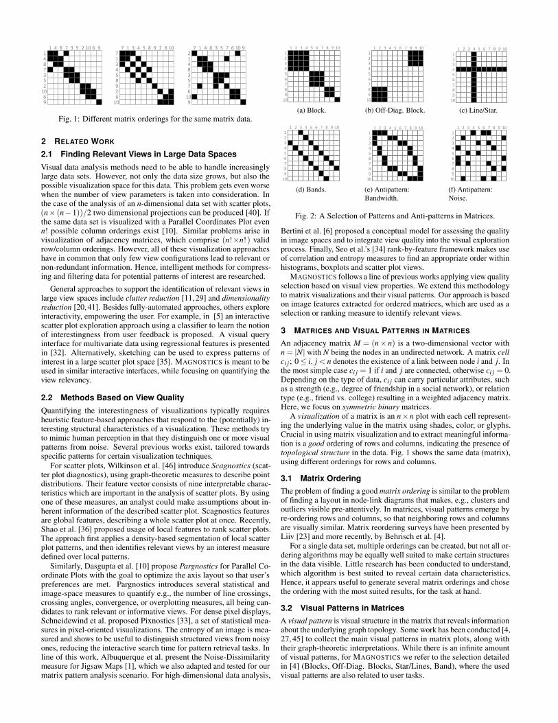
Fig. 1: Different matrix orderings for the same matrix data.

2 RELATED WORK

2.1 Finding Relevant Views in Large Data SpacesVisual data analysis methods need to be able to handle increasinglylarge data sets. However, not only the data size grows, but also thepossible visualization space for this data. This problem gets even worsewhen the number of view parameters is taken into consideration. Inthe case of the analysis of an n-dimensional data set with scatter plots,(n× (n−1))/2 two dimensional projections can be produced [40]. Ifthe same data set is visualized with a Parallel Coordinates Plot evenn! possible column orderings exist [10]. Similar problems arise invisualization of adjacency matrices, which comprise (n!×n!) validrow/column orderings. However, all of these visualization approacheshave in common that only few view configurations lead to relevant ornon-redundant information. Hence, intelligent methods for compress-ing and filtering data for potential patterns of interest are researched.

General approaches to support the identification of relevant views inlarge view spaces include clutter reduction [11, 29] and dimensionalityreduction [20, 41]. Besides fully-automated approaches, others exploreinteractivity, empowering the user. For example, in [5] an interactivescatter plot exploration approach using a classifier to learn the notionof interestingness from user feedback is proposed. A visual queryinterface for multivariate data using regressional features is presentedin [32]. Alternatively, sketching can be used to express patterns ofinterest in a large scatter plot space [35]. MAGNOSTICS is meant to beused in similar interactive interfaces, while focusing on quantifying theview relevancy.

2.2 Methods Based on View QualityQuantifying the interestingness of visualizations typically requiresheuristic feature-based approaches that respond to the (potentially) in-teresting structural characteristics of a visualization. These methods tryto mimic human perception in that they distinguish one or more visualpatterns from noise. Several previous works exist, tailored towardsspecific patterns for certain visualization techniques.

For scatter plots, Wilkinson et al. [46] introduce Scagnostics (scat-ter plot diagnostics), using graph-theoretic measures to describe pointdistributions. Their feature vector consists of nine interpretable charac-teristics which are important in the analysis of scatter plots. By usingone of these measures, an analyst could make assumptions about in-herent information of the described scatter plot. Scagnostics featuresare global features, describing a whole scatter plot at once. Recently,Shao et al. [36] proposed usage of local features to rank scatter plots.The approach first applies a density-based segmentation of local scatterplot patterns, and then identifies relevant views by an interest measuredefined over local patterns.

Similarly, Dasgupta et al. [10] propose Pargnostics for Parallel Co-ordinate Plots with the goal to optimize the axis layout so that user’spreferences are met. Pargnostics introduces several statistical andimage-space measures to quantify e.g., the number of line crossings,crossing angles, convergence, or overplotting measures, all being can-didates to rank relevant or informative views. For dense pixel displays,Schneidewind et al. proposed Pixnostics [33], a set of statistical mea-sures in pixel-oriented visualizations. The entropy of an image is mea-sured and shows to be useful to distinguish structured views from noisyones, reducing the interactive search time for pattern retrieval tasks. Inline of this work, Albuquerque et al. present the Noise-Dissimilaritymeasure for Jigsaw Maps [1], which we also adapted and tested for ourmatrix pattern analysis scenario. For high-dimensional data analysis,

12345678

1 2 3 4 5 6 7 8

910

9 10

(a) Block.

12345678

1 2 3 4 5 6 7 8

910

9 10

(b) Off-Diag. Block.

12345678

1 2 3 4 5 6 7 8

910

9 10

(c) Line/Star.

12345678

1 2 3 4 5 6 7 8

910

9 10

(d) Bands.

12345678

1 2 3 4 5 6 7 8

910

9 10

(e) Antipattern:Bandwidth.

12345678

1 2 3 4 5 6 7 8

910

9 10

(f) Antipattern:Noise.

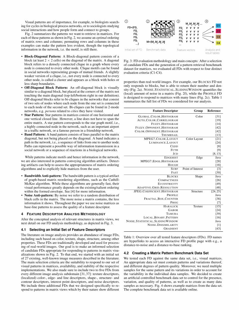
Fig. 2: A Selection of Patterns and Anti-patterns in Matrices.

Bertini et al. [6] proposed a conceptual model for assessing the qualityin image spaces and to integrate view quality into the visual explorationprocess. Finally, Seo et al.’s [34] rank-by-feature framework makes useof correlation and entropy measures to find an appropriate order withinhistograms, boxplots and scatter plot views.

MAGNOSTICS follows a line of previous works applying view qualityselection based on visual view properties. We extend this methodologyto matrix visualizations and their visual patterns. Our approach is basedon image features extracted for ordered matrices, which are used as aselection or ranking measure to identify relevant views.

3 MATRICES AND VISUAL PATTERNS IN MATRICES

An adjacency matrix M = (n× n) is a two-dimensional vector withn = |N| with N being the nodes in an undirected network. A matrix cellci j; 0≤ i, j < n denotes the existence of a link between node i and j. Inthe most simple case ci j = 1 if i and j are connected, otherwise ci j = 0.Depending on the type of data, ci j can carry particular attributes, suchas a strength (e.g., degree of friendship in a social network), or relationtype (e.g., friend vs. college) resulting in a weighted adjacency matrix.Here, we focus on symmetric binary matrices.

A visualization of a matrix is an n×n plot with each cell represent-ing the underlying value in the matrix using shades, color, or glyphs.Crucial in using matrix visualization and to extract meaningful informa-tion is a good ordering of rows and columns, indicating the presence oftopological structure in the data. Fig. 1 shows the same data (matrix),using different orderings for rows and columns.

3.1 Matrix OrderingThe problem of finding a good matrix ordering is similar to the problemof finding a layout in node-link diagrams that makes, e.g., clusters andoutliers visible pre-attentively. In matrices, visual patterns emerge byre-ordering rows and columns, so that neighboring rows and columnsare visually similar. Matrix reordering surveys have been presented byLiiv [23] and more recently, by Behrisch et al. [4].

For a single data set, multiple orderings can be created, but not all or-dering algorithms may be equally well suited to make certain structuresin the data visible. Little research has been conducted to understand,which algorithm is best suited to reveal certain data characteristics.Hence, it appears useful to generate several matrix orderings and chosethe ordering with the most suited results, for the task at hand.

3.2 Visual Patterns in MatricesA visual pattern is visual structure in the matrix that reveals informationabout the underlying graph topology. Some work has been conducted [4,27, 45] to collect the main visual patterns in matrix plots, along withtheir graph-theoretic interpretations. While there is an infinite amountof visual patterns, for MAGNOSTICS we refer to the selection detailedin [4] (Blocks, Off-Diag. Blocks, Star/Lines, Band), where the usedvisual patterns are also related to user tasks.

Visual patterns are of importance, for example, to biologists search-ing for cycles in biological process networks, or to sociologists studyingsocial interactions and how people form and connect to groups.

Fig. 2 summarizes the patterns we want to retrieve in matrices. Foreach of these patterns as shown in Fig. 2, we assume an optimal orderingof matrix rows and columns; permuting rows and columns in theseexamples can make the pattern less evident, though the topologicalinformation in the network, i.e. the motif, is still there.

• Block-Diagonal Pattern: A Block-diagonal pattern consists of ablock (at least 2 × 2 cells) on the diagonal of the matrix. A diagonalblock refers to a densely connected clique in a graph where everynode is connected to every other node. Clique motifs can be foundin social networks representing groups of mutual friends. A slightlyweaker version of a clique, i.e., not every node is connected to everyother node, is called a cluster and appears as a block with holes orless sharp boundaries.

• Off-Diagonal Block Pattern: An off-diagonal block is visuallysimilar to a diagonal block, but placed at the corners of the matrix nottouching the main diagonal (top-left/bottom right in our definition).Off-diagonal blocks refer to bi-cliques in the networks that consistof two sets of nodes where each node from the one set is connectedto each node of the second set. Bi-cliques can be found in 2-modenetworks, e.g. persons related to cities they have visited.

• Star Pattern: Star patterns in matrices consist of one horizontal andone vertical closed line. However, a line does not have to span theentire matrix. A star pattern corresponds to the star graph motif, i.e.,a highly connected node in the network, such as an important airportin a traffic network, or a famous person in a friendship network.

• Band Pattern: A band pattern consists of lines parallel to the matrixdiagonal, but not being placed on the diagonal. A band indicates apath in the network, i.e., a sequence of links from one to another node.Paths can represent a possible way of information transmission in asocial network or a sequence of reactions in a biological networks.

While patterns indicate motifs and hence information in the network,we are also interested in patterns conveying algorithm artifacts. Detect-ing artifacts can help to assess the appropriateness of matrix orderingalgorithms and to explicitly hide matrices from the user.

• Bandwidth Anti-pattern: The bandwidth pattern is a typical artifactof graph-based matrix reordering algorithms, such as the Cuthill-McKee algorithm. While these algorithms are generally fast, theirvisual performance greatly depends on the existing/salient orderingwithin the formed envelope. See [4] for more information.

• Noise Anti-pattern: By noise we refer to a random distribution ofblack cells in the matrix. The more noise a matrix contains, the lessinformation it shows. Throughout the paper we use noise matrices asbase-line patterns to assess the quality of a feature descriptor.

4 FEATURE DESCRIPTOR ANALYSIS METHODOLOGY

After the conceptual analysis of relevant structures in matrix views, wenext detail on our FD analysis methodology, as depicted in Fig. 3.

4.1 Selecting an Initial Set of Feature DescriptorsThe literature on image analysis provides an abundance of image FDs,including such based on color, texture, shape, structure, among otherproperties. These FDs are traditionally developed and used for process-ing of real-world images. Our goal is to make an informed selectionof candidate FDs appropriate for responding to patterns in matrix visu-alizations shown in Fig. 2. To that end, we started with an initial setof 27 existing, well-known image measures described in the literature.The main selection criteria are the suitability to respond to our set ofvisual patterns in matrices, availability, and stability of the respectiveimplementations. We also made sure to include two to five FDs fromevery different image analysis subdomain [31, 37]: texture descriptors,(localized) color-, edge- and line descriptors, shape-, structure- andcontour descriptors, interest point descriptors, and noise descriptors.We include three additional FDs that we designed specifically to re-spond to patterns in matrix views which by their nature show different

1

Initial set of FD

2

Benchmark data

3

Feature vectors

FD={FD FD FD FD FD ...}

1

2

3

4

5 M={M ,M ,M ,M 1 2 3 4

FD FD FD FD FD ...

1

2

3

4

5

M ,M ,M ,M ...1 2 3 4

v v v vv v v vv v v vv v v vv v v v

4

C1

C2

C3

C4

Analysis and result tables

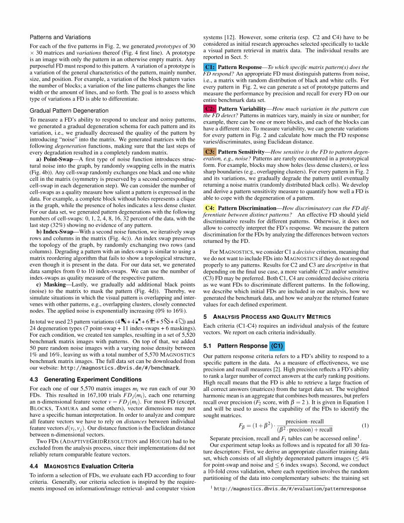
Fig. 3: FD evaluation methodology and main concepts: After a selectionof candidate FDs and the generation of a pattern retrieval benchmarkdataset for matrices, we evaluated all FDs with respect to four distinctevaluation criteria (C1-C4).

properties than real-world images. For example, our BLOCKS FD notonly responds to blocks, but is able to return their number and den-sity (Fig. 2a). NOISE STATISTICAL SLIDINGWINDOW quantifies the(local) amount of noise in a matrix (Fig. 2f), while the PROFILE FDis designed to respond to matrices with many lines (Fig. 2c). Table 1summarizes the full list of FDs we considered for our analysis.

Feature Descriptor Group Reference

GLOBAL COLOR HISTOGRAM Color [31]AUTO COLOR CORRELOGRAM [19]

FUZZY HISTOGRAM [14]FUZZY OPPONENT HISTOGRAM [42]COLOR OPPONENT HISTOGRAM [42]

THUMBNAIL [13]MPEG7 COLOR LAYOUT Color Layout [21]

LUMINANCE LAYOUT [24]CEDD [8]FCTH [9]

JCD [8, 13]EDGEHIST Edge Java

MPEG7 EDGE HISTOGRAM [28]HOUGH [18]

SURF Point of Interest [3]FAST [30]

BLOCKS Shape JavaCOMPACTNESS [26]ECCENTRICITY [49]

ADAPTIVE GRID RESOLUTION [48]JPEG COEFFICIENT HISTOGRAM Structure [24, 25]

PROFILE JavaFRACTAL BOX COUNTER [38]

PHOG [7]HARALICK Texture [15]

GABOR [24]TAMURA [39]

LOCAL BINARY PATTERN [16]NOISE STATISTICAL SLIDINGWINDOW Java

NOISE DISSIMILARITY [1]GRADIENT [43]

Table 1: Overview over all tested feature descriptors (FDs). FD namesare hyperlinks to access an interactive FD profile page with e.g., adistance-to-noise and a distance-to-base ranking.

4.2 Creating a Matrix Pattern Benchmark Data SetWe tested each FD against the same data set, i.e., visual matrices.An appropriate data set must contain patterns and variations thereof,and different degrees of pattern quality. Moreover, we need multiplesamples for the same pattern and its variations in order to account forthe variability in the individual data samples. We decided to createan artificial controlled benchmark data set to control for the presence,variation, and quality of patterns, as well as to create as many datasamples as necessary. Fig. 4 shows example matrices from the data set.The complete benchmark data set is available online.

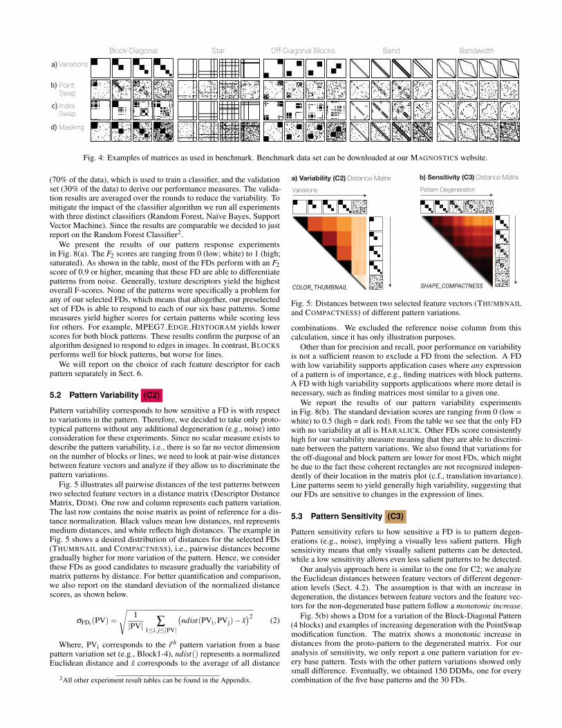
Patterns and VariationsFor each of the five patterns in Fig. 2, we generated prototypes of 30× 30 matrices and variations thereof (Fig. 4 first line). A prototypeis an image with only the pattern in an otherwise empty matrix. Anypurposeful FD must respond to this pattern. A variation of a prototype isa variation of the general characteristics of the pattern, mainly number,size, and position. For example, a variation of the block pattern variesthe number of blocks; a variation of the line patterns changes the linewidth or the amount of lines, and so forth. The goal is to assess whichtype of variations a FD is able to differentiate.

Gradual Pattern DegenerationTo measure a FD’s ability to respond to unclear and noisy patterns,we generated a gradual degeneration schema for each pattern and itsvariation, i.e., we gradually decreased the quality of the pattern byintroducing “noise” into the matrix. We generated matrices with thefollowing degeneration functions, making sure that the last steps ofevery degradation resulted in a completely random matrix.

a) Point-Swap—A first type of noise function introduces struc-tural noise into the graph, by randomly swapping cells in the matrix(Fig. 4b)). Any cell-swap randomly exchanges one black and one whitecell in the matrix (symmetry is preserved by a second correspondingcell-swap in each degeneration step). We can consider the number ofcell-swaps as a quality measure how salient a pattern is expressed in thedata. For example, a complete block without holes represents a cliquein the graph, while the presence of holes indicates a less dense cluster.For our data set, we generated pattern degenerations with the followingnumbers of cell-swaps: 0, 1, 2, 4, 8, 16, 32 percent of the data, with thelast step (32%) showing no evidence of any pattern.

b) Index-Swap—With a second noise function, we iteratively swaprows and columns in the matrix (Fig. 4c)). An index swap preservesthe topology of the graph, by randomly exchanging two rows (andcolumns). Degrading a pattern with an index-swap is similar to using amatrix reordering algorithm that fails to show a topological structure,even though it is present in the data. For our data set, we generateddata samples from 0 to 10 index-swaps. We can use the number ofindex-swaps as quality measure of the respective pattern.

c) Masking—Lastly, we gradually add additional black points(noise) to the matrix to mask the pattern (Fig. 4d)). Thereby, wesimulate situations in which the visual pattern is overlapping and inter-venes with other patterns, e.g., overlapping clusters, closely connectednodes. The applied noise is exponentially increasing (0% to 16%).

In total we used 23 pattern variations (4 + 4 + 6 + 5 + 4 ) and24 degeneration types (7 point-swap + 11 index-swaps + 6 maskings).For each condition, we created ten samples, resulting in a set of 5,520benchmark matrix images with patterns. On top of that, we added50 pure random noise images with a varying noise density between1% and 16%, leaving us with a total number of 5,570 MAGNOSTICSbenchmark matrix images. The full data set can be downloaded fromour website: http://magnostics.dbvis.de/#/benchmark.

4.3 Generating Experiment ConditionsFor each one of our 5,570 matrix images mi we run each of our 30FDs. This resulted in 167,100 trials FD j(mi), each one returningan n-dimensional feature vector v = FD j(mi). For most FD (except,BLOCKS, TAMURA and some others), vector dimensions may nothave a specific human interpretation. In order to analyze and compareall feature vectors we have to rely on distances between individualfeature vectors d(vi,v j). Our distance function is the Euclidean distancebetween n-dimensional vectors.

Two FDs (ADAPTIVEGRIDRESOLUTION and HOUGH) had to beexcluded from the analysis process, since their implementations did notreliably return comparable feature vectors.

4.4 MAGNOSTICS Evaluation CriteriaTo inform a selection of FDs, we evaluate each FD according to fourcriteria. Generally, our criteria selection is inspired by the require-ments imposed on information/image retrieval- and computer vision

systems [12]. However, some criteria (esp. C2 and C4) have to beconsidered as initial research approaches selected specifically to tacklea visual pattern retrieval in matrix data. The individual results arereported in Sect. 5:

C1: Pattern Response—To which specific matrix pattern(s) does theFD respond? An appropriate FD must distinguish patterns from noise,i.e., a matrix with random distribution of black and white cells. Forevery pattern in Fig. 2, we can generate a set of prototype patterns andmeasure the performance by precision and recall for every FD on ourentire benchmark data set.C2: Pattern Variability—How much variation in the pattern can

the FD detect? Patterns in matrices vary, mainly in size or number; forexample, there can be one or more blocks, and each of the blocks canhave a different size. To measure variability, we can generate variationsfor every pattern in Fig. 2 and calculate how much the FD responsevaries/discriminates, using Euclidean distance.

C3: Pattern Sensitivity—How sensitive is the FD to pattern degen-eration, e.g., noise? Patterns are rarely encountered in a prototypicalform. For example, blocks may show holes (less dense clusters), or lesssharp boundaries (e.g., overlapping clusters). For every pattern in Fig. 2and its variations, we gradually degrade the pattern until eventuallyreturning a noise matrix (randomly distributed black cells). We developand derive a pattern sensitivity measure to quantify how well a FD isable to cope with the degeneration of a pattern.

C4: Pattern Discrimination—How discriminatory can the FD dif-ferentiate between distinct patterns? An effective FD should yielddiscriminative results for different patterns. Otherwise, it does notallow to correctly interpret the FD’s response. We measure the patterndiscrimination for the FDs by analyzing the differences between vectorsreturned by the FD.

For MAGNOSTICS, we consider C1 a decisive criterion, meaning thatwe do not want to include FDs into MAGNOSTICS if they do not respondproperly to any patterns. Results for C2 and C3 are descriptive in thatdepending on the final use case, a more variable (C2) and/or sensitive(C3) FD may be preferred. Both C1, C4 are considered decisive criteriaas we want FDs to discriminate different patterns. In the following,we describe which initial FDs are included in our analysis, how wegenerated the benchmark data, and how we analyze the returned featurevalues for each defined experiment.

5 ANALYSIS PROCESS AND QUALITY METRICS

Each criteria (C1-C4) requires an individual analysis of the featurevectors. We report on each criteria individually.

5.1 Pattern Response (C1)

Our pattern response criteria refers to a FD’s ability to respond to aspecific pattern in the data. As a measure of effectiveness, we useprecision and recall measures [2]. High precision reflects a FD’s abilityto rank a larger number of correct answers at the early ranking positions.High recall means that the FD is able to retrieve a large fraction ofall correct answers (matrices) from the target data set. The weightedharmonic mean is an aggregate that combines both measures, but prefersrecall over precision (F2 score, with β = 2 ). It is given in Equation 1and will be used to assess the capability of the FDs to identify thesought matrices.

Fβ = (1+β2) · precision · recall

(β 2 ·precision)+ recall(1)

Separate precision, recall and F1 tables can be accessed online1.Our experiment setup looks as follows and is repeated for all 30 fea-

ture descriptors: First, we derive an appropriate classifier training dataset, which consists of all slightly degenerated pattern images (≤ 4%for point-swap and noise and ≤ 6 index swaps). Second, we conducta 10-fold cross validation, where each repetition involves the randompartitioning of the data into complementary subsets: the training set

1 http://magnostics.dbvis.de/#/evaluation/patternresponse

Variations

Block-Diagonal Star Off-Diagonal Blocks Band Bandwidth

a)

Point

Swapb)

c) Index Swap

d) Masking

Fig. 4: Examples of matrices as used in benchmark. Benchmark data set can be downloaded at our MAGNOSTICS website.

(70% of the data), which is used to train a classifier, and the validationset (30% of the data) to derive our performance measures. The valida-tion results are averaged over the rounds to reduce the variability. Tomitigate the impact of the classifier algorithm we run all experimentswith three distinct classifiers (Random Forest, Naıve Bayes, SupportVector Machine). Since the results are comparable we decided to justreport on the Random Forest Classifier2.

We present the results of our pattern response experimentsin Fig. 8(a). The F2 scores are ranging from 0 (low; white) to 1 (high;saturated). As shown in the table, most of the FDs perform with an F2score of 0.9 or higher, meaning that these FD are able to differentiatepatterns from noise. Generally, texture descriptors yield the highestoverall F-scores. None of the patterns were specifically a problem forany of our selected FDs, which means that altogether, our preselectedset of FDs is able to respond to each of our six base patterns. Somemeasures yield higher scores for certain patterns while scoring lessfor others. For example, MPEG7 EDGE HISTOGRAM yields lowerscores for both block patterns. These results confirm the purpose of analgorithm designed to respond to edges in images. In contrast, BLOCKSperforms well for block patterns, but worse for lines.

We will report on the choice of each feature descriptor for eachpattern separately in Sect. 6.

5.2 Pattern Variability (C2)

Pattern variability corresponds to how sensitive a FD is with respectto variations in the pattern. Therefore, we decided to take only proto-typical patterns without any additional degeneration (e.g., noise) intoconsideration for these experiments. Since no scalar measure exists todescribe the pattern variability, i.e., there is so far no vector dimensionon the number of blocks or lines, we need to look at pair-wise distancesbetween feature vectors and analyze if they allow us to discriminate thepattern variations.

Fig. 5 illustrates all pairwise distances of the test patterns betweentwo selected feature vectors in a distance matrix (Descriptor DistanceMatrix, DDM). One row and column represents each pattern variation.The last row contains the noise matrix as point of reference for a dis-tance normalization. Black values mean low distances, red representsmedium distances, and white reflects high distances. The example inFig. 5 shows a desired distribution of distances for the selected FDs(THUMBNAIL and COMPACTNESS), i.e., pairwise distances becomegradually higher for more variation of the pattern. Hence, we considerthese FDs as good candidates to measure gradually the variability ofmatrix patterns by distance. For better quantification and comparison,we also report on the standard deviation of the normalized distancescores, as shown below.

σFDi(PV) =

√1|PV| ∑

1≤i, j≤|PV|

(ndist(PVi,PVj)− x

)2 (2)

Where, PVi corresponds to the ith pattern variation from a basepattern variation set (e.g., Block1-4), ndist() represents a normalizedEuclidean distance and x corresponds to the average of all distance

2All other experiment result tables can be found in the Appendix.

a) Variability (C2) Distance MatrixVariations

COLOR_THUMBNAIL

Pattern Degeneration

SHAPE_COMPACTNESS

b) Sensitivity (C3) Distance Matrix

Fig. 5: Distances between two selected feature vectors (THUMBNAILand COMPACTNESS) of different pattern variations.

combinations. We excluded the reference noise column from thiscalculation, since it has only illustration purposes.

Other than for precision and recall, poor performance on variabilityis not a sufficient reason to exclude a FD from the selection. A FDwith low variability supports application cases where any expressionof a pattern is of importance, e.g., finding matrices with block patterns.A FD with high variability supports applications where more detail isnecessary, such as finding matrices most similar to a given one.

We report the results of our pattern variability experimentsin Fig. 8(b). The standard deviation scores are ranging from 0 (low =white) to 0.5 (high = dark red). From the table we see that the only FDwith no variability at all is HARALICK. Other FDs score consistentlyhigh for our variability measure meaning that they are able to discrimi-nate between the pattern variations. We also found that variations forthe off-diagonal and block pattern are lower for most FDs, which mightbe due to the fact these coherent rectangles are not recognized indepen-dently of their location in the matrix plot (c.f., translation invariance).Line patterns seem to yield generally high variability, suggesting thatour FDs are sensitive to changes in the expression of lines.

5.3 Pattern Sensitivity (C3)

Pattern sensitivity refers to how sensitive a FD is to pattern degen-erations (e.g., noise), implying a visually less salient pattern. Highsensitivity means that only visually salient patterns can be detected,while a low sensitivity allows even less salient patterns to be detected.

Our analysis approach here is similar to the one for C2; we analyzethe Euclidean distances between feature vectors of different degener-ation levels (Sect. 4.2). The assumption is that with an increase indegeneration, the distances between feature vectors and the feature vec-tors for the non-degenerated base pattern follow a monotonic increase.

Fig. 5(b) shows a DDM for a variation of the Block-Diagonal Pattern(4 blocks) and examples of increasing degeneration with the PointSwapmodification function. The matrix shows a monotonic increase indistances from the proto-pattern to the degenerated matrix. For ouranalysis of sensitivity, we only report a one pattern variation for ev-ery base pattern. Tests with the other pattern variations showed onlysmall difference. Eventually, we obtained 150 DDMs, one for everycombination of the five base patterns and the 30 FDs.

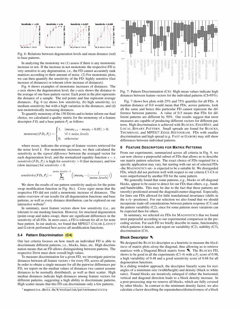
Fig. 6: Relations between degeneration levels and mean distance (red)to base patterns.

In analyzing the monotony we (1) assess if there is any monotonicincrease or not. If the increase in not monotonic the respective FD isvery sensitive to any degeneration, i.e., the FD cannot accurately rankmatrices according to their amount of noise. (2) For monotonic plots,we can then quantify the sensitivity of the FD: highly sensitive (fastincrease of distances) or tolerant (slow increase of distances).

Fig. 6 shows examples of monotonic increases of distances. Thex-axis shows the degeneration level, the y-axis shows the distance tothe average of one base-pattern vector. Each point in the plot representsthe distance of a sample. The red points and line represent averagedistances. Fig. 6 (a) shows low sensitivity, (b) high sensitivity, (c)medium sensitivity but with a high variation in the distances, and (d)non-monotonically increasing distances.

To quantify monotony of the 150 DDMs and to better inform our finalchoice, we calculated a quality metric for the monotony of a featuredescriptor FDi and a base pattern Pj as follows

monotony(FDi,Pj) =

1, (meanl+1−meanl +0.05)> 0;∀l ∈ noise levels.

0, otherwise

where meanl indicates the average of feature vectors retrieved forthe noise level k. For monotonic increases, we then calculated thesensitivity as the signed difference between the averaged vector foreach degeneration level, and the normalized equality function x = y.sensitivity(FDi,Pj) is high for sensitivity > 0 (fast increase), and low(slow increase) for sensitivity < 0.

sensitivity(FDi,Pj) =|noise levels|−1

∑l=0

((meank− (

l|noise levels|

))

We show the results of our pattern sensitivity analysis for the point-swap modification function in Fig. 8(c). Cross signs mean that therespective FD did not yield a monotonic increase of distances. Theentire overview of our results for all degeneration functions and basepatterns, as well as every distance distribution, can be explored on ourinteractive website3.

In summary, most feature vectors show low sensitivity (i.e., aretolerant) to our masking function. However, for structural degeneration(point-swap and index-swap), there are significant differences in thesensitivity of all FDs. In most cases, a FD is tolerant for all or for nonebase pattern. In our analysis, we found that MPEG7 COLOR LAYOUTand GABOR performed best across all modification functions.

5.4 Pattern Discrimination (C4)

Our last criteria focuses on how much an individual FD is able todiscriminate different patterns, i.e., blocks, lines, etc. High discrimi-nation means that an FD allows distinguishing between patterns. Therespective DDM must show overall high values.

To measure discrimination for a given FD, we investigate pairwisedistances between all feature vectors v for every FD, across all patterns.In order to obtain a single measure for all the pairwise differences perFD, we report on the median values of distances (we cannot assumedistances to be normally distributed), as well as their scatter. Highmedian distances indicate high distances among feature vectors fordifferent patterns, suggesting a high ability to discriminate patterns.High scatter means that this FD can discriminate only a few patterns.

3 magnostics.dbvis.de/#/evaluation/patternsensitivity

MPEG7_EDGE_HISTOGRAM

TAM

URACEDDOPPONENT_HISTOGRAM

PHOGM

PEG7_COLOR_LAYOUT AUTO_COLOR_CORRELOGRAM

STATISTICAL_SLIDINGW

INDOW

FRACTAL_BOX_COUNTER PROFILESLOCAL_BINARY_PATTERN JPEGCOEFFICIENTHISTOGRAM

FASTFUZZY_HISTOGRAM

THUM

BNAILGRADIENTCOM

PACTNESS NOISE_DISSIM

ILARITY GLOBALCOLORHISTOGRAM

FCTHBLOCKSLUM

INACE_LAYOUT ECCENTRICITYJCDEDGEHISTGABORFUZZY_OPPONENT_HISTOGRAM

Fig. 7: Pattern Discrimination (C4): High mean values indicate highdistances between feature vectors for the individual patterns (CI=95%).

Fig. 7 shows box plots with 25% and 75% quartiles for all FDs. Amedian distance of 0.0 would mean that FDs, across patterns, lookall the same and hence this particular FD cannot represent the dif-ference between patterns. A value of 0.5 means that FDs for dif-ferent patterns are different by 50%. Our results suggest that mostmeasures are capable of producing different vectors for different pat-terns. High discrimination is achieved with BLOCKS, EDGEHIST, andLOCAL BINARY PATTERN. Small spreads are found for BLOCKS,THUMBNAIL and MPEG7 EDGE HISTOGRAM. FDs with smallerdiscrimination and high spread (e.g. FAST or GABOR) may still showdifferences between individual patterns.

6 FEATURE DESCRIPTORS FOR MATRIX PATTERNS

From our experiments, summarized across all criteria in Fig. 9, wecan now choose a purposeful subset of FDs that allows us to describeour matrix pattern selection. The exact choice of FDs required for aspecific application may vary, but starting with our set of selected FDs–the MAGNOSTICS set– is expected to be a suitable fit. We disregardedFDs, which did not perform well with respect to our criteria C1-C4 orwere outperformed by another FD for the same pattern.

We generally found that some patterns, e.g., blocks or off-diagonalblocks, appear to be easier to detect for our FDs than others, e.g., bandsand bandwidths. This may be due to the fact that these patterns are(mostly) positioned around the diagonal/counter-diagonal. Especially,for lines our FDs allowed for little translational invariance (shifts inthe x-/y- positions). For our selection we also found that we shouldincorporate trade-off considerations between pattern response (C1) andthe pattern variability (C2), since for some patterns more variations canbe expected then for others.

In summary, we selected six FDs for MAGNOSTICS that we foundmost purposeful according to our experimental comparison in the pre-ceding section. For each FD we briefly describe its name, functionality,which patterns it detects, and report on variability (C2), stability (C3),discrimination (C4).

Block DescriptorWe designed the BLOCKS descriptor as a heuristic to measure the block-iness of matrix plots along the diagonal, thus allowing us to retrievematrices with a Diagonal-Block matrix form . The BLOCKS FD,shows to be good in all the experiments (C1-4) with a F2 score of 0.98,a high variability of 0.48 and a good sensitivity score of 0.68 for alldegeneration functions.In a sliding window approach, the descriptor linearly scans for rect-angles of a minimum size (width/height) and density (black to whiteratio). Found blocks are iteratively enlarged if either the horizontal,vertical and diagonal direction leads to a block density increase. Ina post-processing step we remove all blocks, which are fully coveredby other blocks. In contrast to the minimum density factor, we alsocalculate a factor describing the separatedness/distinctiveness of a block

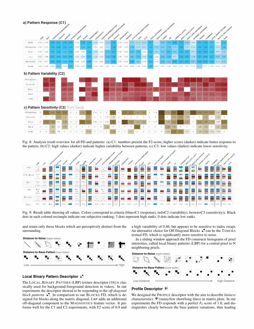
a) Pattern Response (C1)

c) Pattern Sensitivity (C3) Point Swap

b) Pattern Variability (C2)

Fig. 8: Analysis result overview for all FD and patterns: (a) C1: numbers present the F2-score; higher scores (darker) indicate better response tothe pattern, (b) C2: high values (darker) indicate higher variability between patterns, (c) C3: low values (darker) indicate lower sensitivity.

Fig. 9: Result table showing all values. Colors correspond to criteria (blue=C1 (response), red=C2 (variability), brown=C3 (sensitivity)). Blackdots in each colored rectangle indicate our subjective ranking; 3 dots represent high ranks, 0 dots indicate low ranks.

and retain only those blocks which are perceptively distinct from thesurrounding.

Distance-to-Noise (higher better)

Low High

Distance-to-Base-Pattern (lower better)

Local Binary Pattern DescriptorThe LOCAL BINARY PATTERN (LBP) texture descriptor [16] is clas-sically used for background-foreground detection in videos. In ourexperiments the descriptor showed to be responding to the off-diagonalblock patterns . In comparison to our BLOCKS FD, which is de-signed for blocks along the matrix diagonal, LBP adds an additionaloff-diagonal component to the MAGNOSTICS feature vector. It per-forms well for the C1 and C2 experiments, with F2 score of 0.9 and

a high variability of 0.46, but appears to be sensitive to index swaps.An alternative choice for Off-Diagonal Blocks can be the TAMURAtextual FD, which is significantly more sensitive to noise.

In a sliding window approach the FD constructs histograms of pixelintensities, called local binary patterns (LBP) for a central pixel to Nneighboring pixels.

Low Distance High Distance

Distance-to-Noise (higher better)

Distance-to-Base-Pattern (lower better)

Profile Descriptor

We designed the PROFILE descriptor with the aim to describe lininesscharacteristics (many/few short/long lines) in matrix plots. In ourexperiments the FD responds with a perfect F2 score of 1.0, and dis-tinguishes clearly between the base pattern variations, thus leading

to a quite low variability score of 0.28. As all other FDs it reactsmoderately to noise. However, C1 and C2 make this FD especiallysuited for query-by-example search tasks. The PROFILE FD computestwo axis-aligned histograms of the plot, where every matrix row, re-spectively column, represents one histogram bin and the bin’s valuecorresponds the number of black pixels within the respective row. Inorder to achieve translation invariance (i.e., an otherwise empty matrixwith just one row/column line should be equally scored independentof the line’s location) we are computing a standard deviation from theprofile histogram with the intuition that matrix plots with many lineswill show high values, while nearly empty matrices or highly blockymatrices will show low values (few jumps).

Low Distance High Distance

Distance-to-Noise (higher better)

Distance-to-Base-Pattern (lower better)

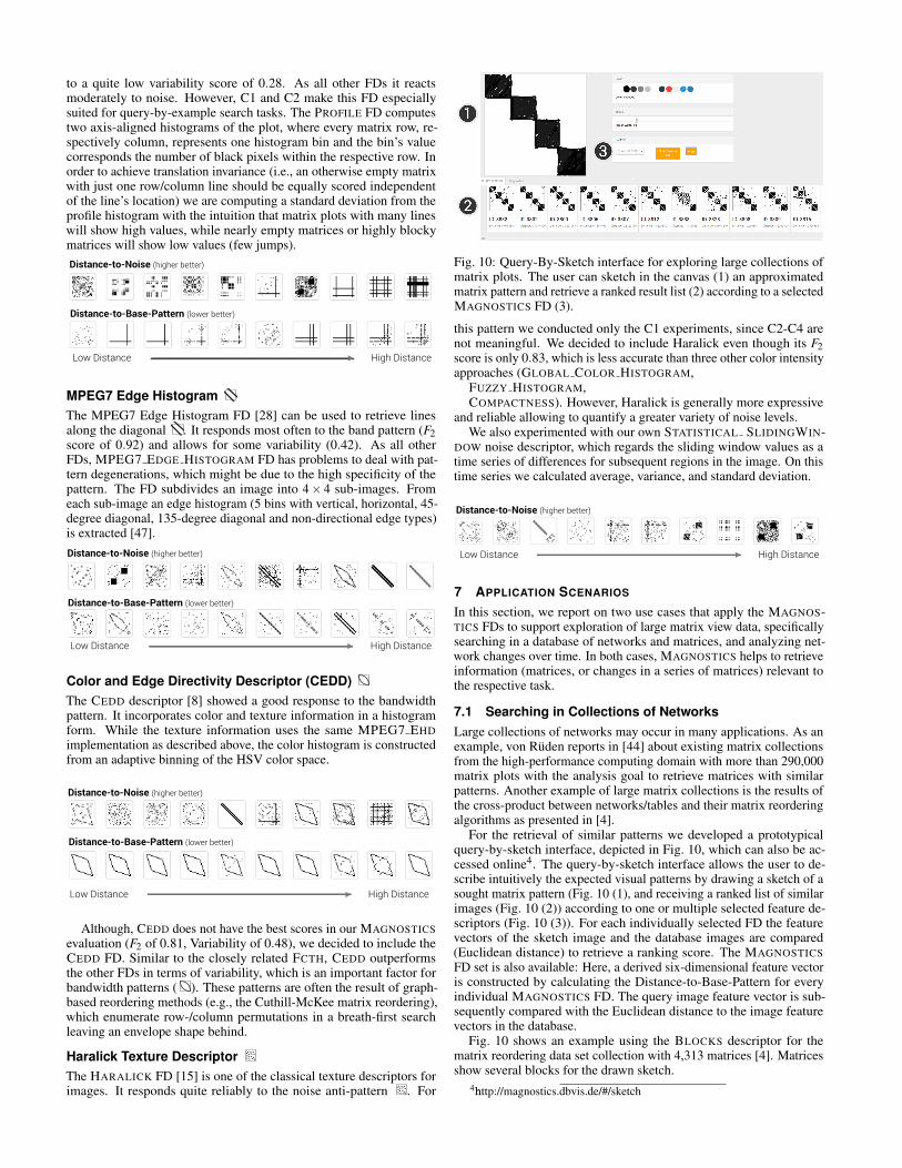
MPEG7 Edge HistogramThe MPEG7 Edge Histogram FD [28] can be used to retrieve linesalong the diagonal . It responds most often to the band pattern (F2score of 0.92) and allows for some variability (0.42). As all otherFDs, MPEG7 EDGE HISTOGRAM FD has problems to deal with pat-tern degenerations, which might be due to the high specificity of thepattern. The FD subdivides an image into 4× 4 sub-images. Fromeach sub-image an edge histogram (5 bins with vertical, horizontal, 45-degree diagonal, 135-degree diagonal and non-directional edge types)is extracted [47].

Low Distance High Distance

Distance-to-Noise (higher better)

Distance-to-Base-Pattern (lower better)

Color and Edge Directivity Descriptor (CEDD)The CEDD descriptor [8] showed a good response to the bandwidthpattern. It incorporates color and texture information in a histogramform. While the texture information uses the same MPEG7 EHDimplementation as described above, the color histogram is constructedfrom an adaptive binning of the HSV color space.

Low Distance High Distance

Distance-to-Noise (higher better)

Distance-to-Base-Pattern (lower better)

Although, CEDD does not have the best scores in our MAGNOSTICSevaluation (F2 of 0.81, Variability of 0.48), we decided to include theCEDD FD. Similar to the closely related FCTH, CEDD outperformsthe other FDs in terms of variability, which is an important factor forbandwidth patterns ( ). These patterns are often the result of graph-based reordering methods (e.g., the Cuthill-McKee matrix reordering),which enumerate row-/column permutations in a breath-first searchleaving an envelope shape behind.

Haralick Texture DescriptorThe HARALICK FD [15] is one of the classical texture descriptors forimages. It responds quite reliably to the noise anti-pattern . For

Fig. 10: Query-By-Sketch interface for exploring large collections ofmatrix plots. The user can sketch in the canvas (1) an approximatedmatrix pattern and retrieve a ranked result list (2) according to a selectedMAGNOSTICS FD (3).

this pattern we conducted only the C1 experiments, since C2-C4 arenot meaningful. We decided to include Haralick even though its F2score is only 0.83, which is less accurate than three other color intensityapproaches (GLOBAL COLOR HISTOGRAM,

FUZZY HISTOGRAM,COMPACTNESS). However, Haralick is generally more expressive

and reliable allowing to quantify a greater variety of noise levels.We also experimented with our own STATISTICAL SLIDINGWIN-

DOW noise descriptor, which regards the sliding window values as atime series of differences for subsequent regions in the image. On thistime series we calculated average, variance, and standard deviation.

Low Distance High Distance

Distance-to-Noise (higher better)

7 APPLICATION SCENARIOS

In this section, we report on two use cases that apply the MAGNOS-TICS FDs to support exploration of large matrix view data, specificallysearching in a database of networks and matrices, and analyzing net-work changes over time. In both cases, MAGNOSTICS helps to retrieveinformation (matrices, or changes in a series of matrices) relevant tothe respective task.

7.1 Searching in Collections of NetworksLarge collections of networks may occur in many applications. As anexample, von Ruden reports in [44] about existing matrix collectionsfrom the high-performance computing domain with more than 290,000matrix plots with the analysis goal to retrieve matrices with similarpatterns. Another example of large matrix collections is the results ofthe cross-product between networks/tables and their matrix reorderingalgorithms as presented in [4].

For the retrieval of similar patterns we developed a prototypicalquery-by-sketch interface, depicted in Fig. 10, which can also be ac-cessed online4. The query-by-sketch interface allows the user to de-scribe intuitively the expected visual patterns by drawing a sketch of asought matrix pattern (Fig. 10 (1), and receiving a ranked list of similarimages (Fig. 10 (2)) according to one or multiple selected feature de-scriptors (Fig. 10 (3)). For each individually selected FD the featurevectors of the sketch image and the database images are compared(Euclidean distance) to retrieve a ranking score. The MAGNOSTICSFD set is also available: Here, a derived six-dimensional feature vectoris constructed by calculating the Distance-to-Base-Pattern for everyindividual MAGNOSTICS FD. The query image feature vector is sub-sequently compared with the Euclidean distance to the image featurevectors in the database.

Fig. 10 shows an example using the BLOCKS descriptor for thematrix reordering data set collection with 4,313 matrices [4]. Matricesshow several blocks for the drawn sketch.

4http://magnostics.dbvis.de/#/sketch

4 5 6 7 148 9 121110 13 15

Dist

ance

to s

ucce

ssor

Fig. 11: Detail from a dynamic network representing brain connectivity(300 time records).

7.2 Dynamic Network AnalysisAnother challenge in the realm of large data collections are networkschanging over time; every time step represents the network at a differenttime instance. Fig. 11 shows 11 matrices from a dynamic brain connec-tivity network, usually comprising around 300 time points (individualmatrices). Brain connectivity refers to the co-variance (connection)between activity in brain regions (regions of interest, ROI). Neuroscien-tists are specifically interested in clusters (Blocks) and their evolution,as well as in identifying noisy time periods. Here, a time point repre-sents 2-seconds, and dark cells indicate high connectivity (binarized toobtain un-weighted network). Rows and columns in the matrices areordered to optimize the visual patterns independently for each matrix.

To find time points with major changes with respect to noise andblocks, we first calculate a feature vector vi for every matrix (timepoint) ti with HARALICK (noise) and another one with BLOCKS. Then,we calculate the difference for each feature vector vi and the followingtime step vi+1 (separately for both HARALICK and BLOCKS). Highdistances indicate high changes between two consecutive time points,low distances indicate little change (with respect to noise).

Fig. 11 shows both distances plotted (red=BLOCKS,blue=HARALICK). For noise we can observe major differ-ences between time points 11-14, while the type of blocks changesmost between time points 6-8. Both changes are observable in therespective matrices. Further, we observe, between 9 and 15, a constantchange (constant distances) for the BLOCKS FD (red), indicating asalient trend; a possible explanation could be the change from twoseparate blocks (clusters) to one larger block.

8 DISCUSSION AND EXTENSIONS

Quantifying patterns in visualizations is an active research field withvarying approaches. While pattern measures can also be derived fromthe data space, in our case by graph analysis, MAGNOSTICS followsthe idea to take advantage of screen-space measures. This has theadvantage that a direct correspondence to the human perceptual systemcan be constructed.

With MAGNOSTICS we propose an initial set of feature descrip-tors which showed appropriate based on certain desirable criteria (seeSect. 4.4) and showed useful to support ranking, searching and cluster-ing of matrices (see Sect. 7).

8.1 Defining and Retrieving Interesting Matrix ViewsWhile we have focused on six specific patterns and their variations, webelieve our criteria and methodology from Sect. 4 will allow for theselection of FDs for different patterns including directed and weightednetworks, as well as application specific patterns. Also, higher-levelvisual characteristics of matrices, such as the degree of “clumpy-ness”could be investigated with our MAGNOSTICS evaluation approach.

Further criteria for an effective MAGNOSTICS FD could also beconsidered. For example, the human users’ assessment of featuredescriptor quality in light of matrix exploration tasks could influencethe FD selection process in a user-centric fashion. For example, linesmay still be visible to humans, though the algorithms may not detectthem and vice versa. It may also be interesting to link MAGNOSTICSanalysis with interactive matrix exploration techniques. For example,

the NodeTrix approach [17] includes node-link views aside the matrices,hence we would also need to include FDs for node-link views to jointlyrank interesting views.

A scenario we have not followed further, but which is describedin Scagnostics [46], is to present matrix views that are most differentfrom the others, i.e., outlier views. Since MAGNOSTICS is based on thedistances between feature vectors, it is straightforward to cluster matrixviews based on the feature-vector distances and to report on morecommon views and outliers. Finally, MAGNOSTICS can be embeddedin interactive approaches, in that FDs get weighted either explicitly bythe user, or implicitly by a function analyzing an user’s preferenceswhile navigating the matrix space.

Given that FDs and their corresponding distance functions are thebasis for many data analysis tasks, more application scenarios as thepresented can be supported. In this work we considered ranking andsearching tasks. Other potentially useful applications include the clas-sification of matrix views according to expected classes, according touser interest or the clustering of matrix views.

8.2 Novel Image Measures for Matrix Diagnostics

Another open question remains the development of novel feature de-scriptors for matrices. As described in the previous section, there maybe more visual patterns important to users of matrix analysis. Whileour FDs are global, a natural extension would be to consider local FDs,focussing on specific subnetworks. Furthermore, we considered adja-cency (binary) matrices, but MAGNOSTICS could be extended with FDsalso for continuous matrices (e.g., representing weighted networks).

Finally, we mention that the MAGNOSTICS framework can easilybe applied to evaluate existing matrix reordering algorithms in termsof the visual patterns they produce. Our approach could even informthe design of new reordering algorithms which aim to optimize matrixviews for certain user-dependent patterns of interest.

9 CONCLUSION

We introduced MAGNOSTICS, an experimentally validated set of viewdescriptors aiming to guide exploration of large network collections,represented as matrix views. Starting from a set of 30 feature descrip-tors, including three novel specifically designed FDs, we identified aset of six useful FDs for the analysis of visual patterns in matrices.The selection of descriptors was guided by a structured and explo-rative methodology, using a novel large matrix benchmark data setand based on four quantifiable criteria: (1) pattern response, (2) pat-tern similarity, (3) pattern sensitivity and (4) pattern discrimination.We demonstrated how MAGNOSTICS can be applied in an interactiveranking and searching tasks, and to analyze time series of networks.MAGNOSTICS complements the set of previous feature-based analysisframeworks in the context of Visual Analytics tools.

ACKNOWLEDGMENTS

The authors wish to thank Nayeem Khan for the discussions that con-tributed to this work. We also thank Bianca Orita, Manuel Hotz andRaffael Wagner for the development of the block feature descriptorand the statistical noise descriptor. The authors thank the GermanResearch Foundation (DFG) for financial support within project A03“Quantification of Visual Analytics Transformations and Mappings” ofSFB/Transregio 161.

REFERENCES

[1] G. Albuquerque, M. Eisemann, D. J. Lehmann, H. Theisel, and M. Magnor.Improving the visual analysis of high-dimensional datasets using qualitymeasures. In Visual Analytics Science and Technology (VAST), 2010 IEEESymposium on, pp. 19–26. IEEE, 2010.

[2] R. A. Baeza-Yates and B. A. Ribeiro-Neto. Modern Information Retrieval- the concepts and technology behind search, Second edition. PearsonEducation Ltd., Harlow, England, 2011.

[3] H. Bay, A. Ess, T. Tuytelaars, and L. Van Gool. Speeded-up robust features(surf). Computer Vision and Image Understanding, 110(3):346–359, June2008. doi: 10.1016/j.cviu.2007.09.014

[4] M. Behrisch, B. Bach, N. H. Riche, T. Schreck, and J.-D. Fekete. MatrixReordering Methods for Table and Network Visualization. ComputerGraphics Forum, 2016. doi: 10.1111/cgf.12935

[5] M. Behrisch, F. Korkmaz, L. Shao, and T. Schreck. Feedback-driveninteractive exploration of large multidimensional data supported by visualclassifier. In Proc. IEEE Conference on Visual Analytics Science andTechnology, pp. 43–52, 2014. doi: 10.1109/VAST.2014.7042480

[6] E. Bertini, A. Tatu, and D. A. Keim. Quality Metrics in High-DimensionalData Visualization: An Overview and Systematization. IEEE Symp. onInformation Visualization (InfoVis), 17(12):2203–2212, Dec. 2011.

[7] A. Bosch, A. Zisserman, and X. Munoz. Representing shape with a spatialpyramid kernel. In Proc. of the 6th ACM International Conference onImage and Video Retrieval, pp. 401–408. ACM, 2007.

[8] S. A. Chatzichristofis and Y. S. Boutalis. Cedd: color and edge directivitydescriptor: a compact descriptor for image indexing and retrieval. InComputer vision systems, pp. 312–322. Springer, 2008.

[9] S. A. Chatzichristofis and Y. S. Boutalis. Fcth: Fuzzy color and texturehistogram - a low level feature for accurate image retrieval. In ImageAnalysis for Multimedia Interactive Services, 2008. WIAMIS ’08. 9th Int.Workshop on, pp. 191–196, May 2008. doi: 10.1109/WIAMIS.2008.24

[10] A. Dasgupta and R. Kosara. Pargnostics: Screen-space metrics for parallelcoordinates. IEEE Transactions on Visualization and Computer Graphics,16(6):1017–1026, 2010.

[11] G. Ellis and A. Dix. A taxonomy of clutter reduction for informationvisualisation. IEEE Transactions on Visualization and Computer Graphics,13(6):1216–1223, 2007. doi: 10.1109/TVCG.2007.70535

[12] R. Gonzalez and R. Woods. Digital Image Processing. Pearson/PrenticeHall, 2008.

[13] F. Graf. Jfeaturelib v1.6.3, Sept. 2015. doi: 10.5281/zenodo.31793[14] J. Han and K.-K. Ma. Fuzzy color histogram and its use in color image

retrieval. Image Processing, IEEE Transactions on, 11(8):944–952, 2002.[15] R. Haralick, K. Shanmugam, and I. Dinstein. Textural features for image

classification. Systems, Man and Cybernetics, IEEE Transactions on,SMC-3(6):610–621, Nov 1973. doi: 10.1109/TSMC.1973.4309314

[16] M. Heikkl and M. Pietikinen. A texture-based method for modeling thebackground and detecting moving objects. IEEE transactions on patternanalysis and machine intelligence, 28(4):657–62, 2006.

[17] N. Henry, J.-D. Fekete, and M. J. McGuffin. NodeTrix: a hybrid visualiza-tion of social networks. IEEE transactions on visualization and computergraphics, 13(6):1302–9, 2007. doi: 10.1109/TVCG.2007.70582

[18] P. Hough. Method and means for recognizing complex patterns, Dec 1962.[19] J. Huang, S. R. Kumar, M. Mitra, W.-J. Zhu, and R. Zabih. Image indexing

using color correlograms. In Computer Vision and Pattern Recognition,Proc. of IEEE Conference on, pp. 762–768, Jun 1997. doi: 10.1109/CVPR.1997.609412

[20] S. Ingram, T. Munzner, V. Irvine, M. Tory, S. Bergner, and T. Moller.Dimstiller: Workflows for dimensional analysis and reduction. In Proc. ofthe IEEE Conference on Visual Analytics Science and Technology, IEEEVAST,, pp. 3–10, 2010. doi: 10.1109/VAST.2010.5652392

[21] E. Kasutani and A. Yamada. The mpeg-7 color layout descriptor: acompact image feature description for high-speed image/video segmentretrieval. In Image Processing, 2001. Proceedings. 2001 Int. Conferenceon, vol. 1, pp. 674–677 vol.1, 2001. doi: 10.1109/ICIP.2001.959135

[22] D. J. Lehmann, F. Kemmler, T. Zhyhalava, M. Kirschke, and H. Theisel.Visualnostics: Visual guidance pictograms for analyzing projections ofhigh-dimensional data. In Computer Graphics Forum, vol. 34, pp. 291–300. Wiley Online Library, 2015.

[23] I. Liiv. Seriation and matrix reordering methods: An historical overview.Statistical analysis and data mining, 3(2):70–91, 2010.

[24] M. Lux and S. A. Chatzichristofis. Lire: Lucene image retrieval: Anextensible java cbir library. In Proceedings of the 16th ACM InternationalConference on Multimedia, MM ’08, pp. 1085–1088. ACM, New York,NY, USA, 2008. doi: 10.1145/1459359.1459577

[25] M. Lux, A. Pitman, and O. Marques. Callisto: Tag recommendations byimage content. WISMA 2010, p. 87, 2010.

[26] B. S. Morse. Lecture 9: Shape description (regions).[27] C. Mueller, B. Martin, and a. Lumsdaine. Interpreting large visual similar-

ity matrices. 2007 6th International Asia-Pacific Symposium on Visualiza-tion, pp. 149–152, Feb. 2007. doi: 10.1109/APVIS.2007.329290

[28] D. K. Park, Y. S. Jeon, and C. S. Won. Efficient use of local edge histogramdescriptor. In Proceedings of the 2000 ACM Workshops on Multimedia,MULTIMEDIA ’00, pp. 51–54. ACM, New York, NY, USA, 2000. doi:10.1145/357744.357758

[29] W. Peng, M. O. Ward, and E. A. Rundensteiner. Clutter reduction in multi-dimensional data visualization using dimension reordering. In InformationVisualization. INFOVIS 2004. IEEE Symp., pp. 89–96. IEEE, 2004.

[30] E. Rosten, R. Porter, and T. Drummond. Faster and better: A machinelearning approach to corner detection. IEEE Trans. Pattern Analysis andMachine Intelligence, 32:105–119, 2010. doi: 10.1109/TPAMI.2008.275

[31] Y. Rui, T. S. Huang, and S.-F. Chang. Image retrieval: Current techniques,promising directions, and open issues. Journal of visual communicationand image representation, 10(1):39–62, 1999.

[32] M. Scherer, J. Bernard, and T. Schreck. Retrieval and exploratory searchin multivariate research data repositories using regressional features. InProceedings of the 11th annual international ACM/IEEE joint conferenceon Digital libraries, pp. 363–372. ACM, 2011.

[33] J. Schneidewind, M. Sips, and D. A. Keim. Pixnostics: Towards measuringthe value of visualization. In Visual Analytics Science And Technology,2006 IEEE Symposium On, pp. 199–206. IEEE, 2006.

[34] J. Seo and B. Shneiderman. A rank-by-feature framework for unsupervisedmultidimensional data exploration using low dimensional projections. InInformation Visualization, 2004. INFOVIS 2004. IEEE Symposium on, pp.65–72, 2004. doi: 10.1109/INFVIS.2004.3

[35] L. Shao, M. Behrisch, T. Schreck, T. von Landesberger, M. Scherer,S. Bremm, and D. A. Keim. Guided Sketching for Visual Search andExploration in Large Scatter Plot Spaces. In M. Pohl and J. Roberts, eds.,Proc. EuroVA International Workshop on Visual Analytics. The Eurograph-ics Association, 2014. doi: 10.2312/eurova.20141140

[36] L. Shao, T. Schleicher, M. Behrisch, T. Schreck, I. Sipiran, and D. Keim.Guiding the exploration of scatter plot data using motif-based interestmeasures. In IEEE Int. Symposium on Big Data Visual Analytics, 2015.

[37] A. W. Smeulders, M. Worring, S. Santini, A. Gupta, and R. Jain. Content-based image retrieval at the end of the early years. Pattern Analysis andMachine Intelligence, IEEE Transactions on, 22(12):1349–1380, 2000.

[38] T. Smith, G. Lange, and W. Marks. Fractal methods and results in cel-lular morphologydimensions, lacunarity and multifractals. Journal ofneuroscience methods, 69(2):123–136, 1996.

[39] H. Tamura, S. Mori, and T. Yamawaki. Textural features corresponding tovisual perception. IEEE Transactions on Systems, Man, and Cybernetics,8(6):460–473, June 1978. doi: 10.1109/TSMC.1978.4309999

[40] A. Tatu, G. Albuquerque, M. Eisemann, P. Bak, H. Theisel, M. A. Magnor,and D. A. Keim. Automated analytical methods to support visual explo-ration of high-dimensional data. IEEE Transactions on Visualization andComputer Graphics, 17(5):584–597, 2011.

[41] A. Tatu, F. Maas, I. Farber, E. Bertini, T. Schreck, T. Seidl, and D. Keim.Subspace search and visualization to make sense of alternative clusteringsin high-dimensional data. In Visual Analytics Science and Technology(VAST), 2012 IEEE Conference on, pp. 63–72. IEEE, 2012.

[42] K. van de Sande, T. Gevers, and C. Snoek. Evaluating color descriptors forobject and scene recognition. Pattern Analysis and Machine Intelligence,IEEE Trans. on, 32(9):1582 –1596, sept. 2010. doi: 10.1109/TPAMI.2009.154

[43] L. von Ruden. Visual analytics of parallel-performance data: Automaticidentification of relevant and similar data subsets. Master’s thesis, RWTHAachen University, April 2015.

[44] L. von Ruden, M.-A. Hermanns, M. Behrisch, D. A. Keim, B. Mohr, andF. Wolf. Separating the wheat from the chaff: Identifying relevant andsimilar performance data with visual analytics. In Proc. of the 2nd Work-shop on Visual Performance Analysis (VPA), Supercomputing Conference2015, pp. 4:1–4:8. ACM, 2015. doi: 10.1145/2835238.2835242

[45] L. Wilkinson. The Grammar of Graphics (Statistics and Computing).Springer-Verlag New York, Inc., Secaucus, NJ, USA, 2005.

[46] L. Wilkinson, A. Anand, and R. Grossman. Graph-theoretic scagnostics.In Proceedings of the Proceedings of the 2005 IEEE Symposium on In-formation Visualization, INFOVIS ’05, pp. 21–. IEEE Computer Society,Washington, DC, USA, 2005. doi: 10.1109/INFOVIS.2005.14

[47] C. S. Won. Adv. in Multimedia Information Processing - PCM 2004: 5thPacific Rim Conference on Multimedia, Tokyo, Japan, 2004. Proceedings,Part III, chap. Feature Extraction and Evaluation Using Edge HistogramDescriptor in MPEG-7, pp. 583–590. Springer, 2005. doi: 10.1007/978-3-540-30543-9 73

[48] M. Yang, K. Kpalma, and J. Ronsin. A Survey of Shape Feature ExtractionTechniques. Peng-Yeng Yin, 2008.

[49] I. T. Young, J. E. Walker, and J. E. Bowie. An analysis technique forbiological shape. i. Information and control, 25(4):357–370, 1974.