β-convergence stability among “old” and “new” eu countries

1

Mariusz Próchniak1, Bartosz Witkowski2

β-Convergence Stability Among “Old” and “New” EU Countries: The

Bayesian Model Averaging Perspective3

1. Introduction

In the literature there are many definitions of real economic convergence as well as many

methods used in verifying the convergence hypothesis. For example Islam (2003)

distinguishes 7 types of classifications: (a) convergence within a given economy and

convergence between economies, (b) convergence of growth rates and convergence of income

levels, (c) β and σ convergence, (d) absolute and conditional convergence, (e) global and

local convergence, (f) GDP and TFP convergence, (g) deterministic and stochastic

convergence. The concept of income-level or real convergence is widely used by economists.

Many theoretical and empirical papers on this subject have emerged in recent years. However,

the lack of both one definition of convergence and one method of analyzing this phenomenon

yielded a huge diversity of the empirical evidence. The conclusions obtained by various

authors depend to a large extent on the analyzed sample of countries, the model specification,

and the estimation method.

When conducting empirical studies on convergence two problems with the standard

approach may be identified. The first one is the stability of the parameters over time. In most

empirical studies it is assumed that the impact of a given variable (the initial income level or

any other economic growth determinant) is treated as stable over time. It means that the

coefficient standing for a given variable is calculated as one value valid for the entire period.

Such a model specification, however, does not provide us with the full picture of the factors

determining the pace of economic growth. The real world is very complicated, driven by

many mechanisms and affected by many shocks, both from the inside and outside sources, so

there are no reasons to assume a priori that the relationships between the macroeconomic

1 Szkoła Główna Handlowa w Warszawie, Katedra Ekonomii II, Kolegium Gospodarki Światowej; e-mail: [email protected]. 2 Szkoła Główna Handlowa w Warszawie, Instytut Ekonometrii, Kolegium Analiz Ekonomicznych; e-mail: [email protected]. 3 This research project has been financed by the National Bank of Poland within the frame of the competition for research grants scheduled for 2012.

2

variables are constant over time.

The second problem deals with the set of explanatory variables, treated as economic

growth determinants. Even in the case of the same sample and the same method of

econometric modeling, the inclusion of different sets of explanatory variables in the

regression model often yields different, not to say contradictory results. Sala-i-Martin,

Doppelhofer, and Miller (2004, SDM hereafter) try to solve this problem using a new

approach: Bayesian averaging of classical estimates (BACE). Instead of using one model,

they estimate a large number of equations corresponding to all possible sets of explanatory

variables chosen from an initially selected group of ‘candidate-variables’. The results are then

averaged using specified weights.

This study tries to shed some light on these doubts and questions. The aims of this analysis

are twofold. The first aim is to check whether the pace of convergence of the European Union

(EU) countries were constant or variable over time. As it is a priori expected the variability

over time, the study tries to indicate the periods when the catching up process was faster as

well as those when the countries caught up slower. Second, the paper focuses on the analysis

of the time stability of the impact of selected macroeconomic variables on economic growth.

The analysis includes a number of robustness tests. First, the calculations are carried out

separately for the whole group of the 27 EU countries (EU27) as well as for the narrower

group of the 15 old EU members (EU15). The calculations for EU15 cover the 1972-2010

period while the calculations for EU27 countries include the years 1993-2010. Second, the

model estimations are based on two different types of time series transformation: data

averaged into 3-year subperiods and panel data.

The study incorporates the innovative Bayesian model averaging (BMA) method applied

to Blundell and Bond’s GMM system estimator. Moreover, this modeling is extended by

allowing for structural breaks of some of the variables to assess the turning points and to show

whether the impact of a given variable on the pace of economic growth was constant over

time.

Although the research method refers to the Bayesian model averaging, this study is not the

pure replica of the analysis conducted by SDM or any other authors. It may be rather treated

as a very interesting extension and supplement to the existing studies incorporating Bayesian

modeling. This research yields a large scope of new knowledge on the sources of economic

growth and its stability over time. The main differences are the following. First, this analysis

does not incorporate the BACE approach; the Bayesian model averaging is applied not to the

classical estimates but to a much more advanced Blundell and Bond’s GMM system estimator

3

which seems to be a better one in analyzing economic growth determinants and real

convergence. Second, unlike SDM, this study is based on 3-year intervals and panel data

meaning that the results should be more representative than those obtained on cross-sectional

data. Third, the research focuses not only on identifying the most important economic growth

determinants but mainly – what is innovative also in comparison with many other empirical

studies – on the analysis of convergence. It is assumed that real convergence does occur and

the initial income level appears in all the estimated regression equations which may be

regarded as a novum in terms of the existing studies incorporating BMA or BACE

approaches. Last but not least, this study deals with identifying the stability of the examined

relationships over time by checking whether convergence occurred at constant or variable

rates during the analyzed period; the same concerns the selected economic growth

determinants.

The paper is composed of six parts. Chapter 2 which appears just after this introduction

shows the theoretical issues related with β convergence and presents the review of the

literature in the context of convergence and Bayesian model averaging. Section 3 presents the

general idea of BMA and BACE modeling and describe the convergence model with

nonstability. Chapter 4 presents the data used. The results of the analysis are discussed in

chapter 5. Section 6 concludes.

2. Theoretical and empirical background

The concepts of real convergence most often used in empirical studies are the following: β

convergence and σ convergence. β convergence exists if the GDP of less developed countries

(with lower GDP per capita) grows faster than the GDP of more developed ones. This type of

convergence can be analyzed in absolute or conditional terms. Absolute convergence means

that less developed countries always reveal higher economic growth while conditional

convergence confirms the catching-up process only for those countries that tend to reach the

same steady state (which – in general – need not be the same across all economies). σ

convergence exists if the differentiation of the GDP per capita levels between economies

(measured e.g. by standard deviation of log GDP per capita) decreases over time.

The concept of β convergence is directly related with neoclassical models of economic

growth (see e.g. Solow 1956; Mankiw, Romer, Weil 1992). The main factor responsible for

equalization of income levels is the neoclassical assumption of diminishing returns to capital.

Countries which are capital scarce obtain higher productivity of that input. That, in turn,

4

stimulates the investments processes and enhances rapid economic growth.

The concept of convergence can be explained based on the Solow model. The main

equation describing the dynamics of the economy is:

, (1)

where: k(t) – capital per unit of effective labor, – the increase of k per unit of time (the

time derivative of k), f(.) – output per unit of effective labor, n – population growth, a –

technological progress, δ – depreciation rate, t – time. Assuming that the neoclassical

production function if of the Cobb-Douglas form f(k) = kα, after dividing equation (1) by k we

get:

. (2)

The above equation shows the growth rate of capital per unit of effective labor during the

transition period in the Solow model. Since output is proportional to capital, the growth

trajectory given by (1) or (2) can also be interpreted in GDP terms.

Equation (2) can be used to show the concept of convergence. The derivative of with

respect to k equals:

. (3)

The above expression is negative which means that the rate of economic growth decreases

with income level (i.e. higher per capita income implies slower GDP growth). This suggests

the existence of real economic β convergence.

The catching-up process confirmed by neoclassical models is not absolute. Suppose the

existence of two separate economies. If both of them approach different steady states, less

developed economy need not grow faster. The possibility of such an outcome indicates that

the convergence explained by neoclassical models of economic growth is conditional, that is

it occurs with regard to individual steady states to which the countries are tending. The

respective neoclassical models of economic growth differ, however, in terms of the value of

the β coefficient. This coefficient indicates the rate of the catching-up process, according to

the following equation:

, (4)

where: y – GDP per capita in the period t, y* – GDP per capita in the steady state. Equation

(4) implies that the rate of economic growth depends on the income gap with respect to the

5

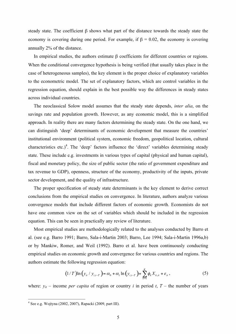
steady state. The coefficient β shows what part of the distance towards the steady state the

economy is covering during one period. For example, if β = 0.02, the economy is covering

annually 2% of the distance.

In empirical studies, the authors estimate β coefficients for different countries or regions.

When the conditional convergence hypothesis is being verified (that usually takes place in the

case of heterogeneous samples), the key element is the proper choice of explanatory variables

to the econometric model. The set of explanatory factors, which are control variables in the

regression equation, should explain in the best possible way the differences in steady states

across individual countries.

The neoclassical Solow model assumes that the steady state depends, inter alia, on the

savings rate and population growth. However, as any economic model, this is a simplified

approach. In reality there are many factors determining the steady state. On the one hand, we

can distinguish ‘deep’ determinants of economic development that measure the countries’

institutional environment (political system, economic freedom, geopolitical location, cultural

characteristics etc.)4. The ‘deep’ factors influence the ‘direct’ variables determining steady

state. These include e.g. investments in various types of capital (physical and human capital),

fiscal and monetary policy, the size of public sector (the ratio of government expenditure and

tax revenue to GDP), openness, structure of the economy, productivity of the inputs, private

sector development, and the quality of infrastructure.

The proper specification of steady state determinants is the key element to derive correct

conclusions from the empirical studies on convergence. In literature, authors analyze various

convergence models that include different factors of economic growth. Economists do not

have one common view on the set of variables which should be included in the regression

equation. This can be seen in practically any review of literature.

Most empirical studies are methodologically related to the analyses conducted by Barro et

al. (see e.g. Barro 1991; Barro, Sala-i-Martin 2003; Barro, Lee 1994; Sala-i-Martin 1996a,b)

or by Mankiw, Romer, and Weil (1992). Barro et al. have been continuously conducting

empirical studies on economic growth and convergence for various countries and regions. The

authors estimate the following regression equation:

, (5)

where: yit – income per capita of region or country i in period t, T – the number of years

4 See e.g. Wojtyna (2002, 2007), Rapacki (2009, part III).

6

covered by one observation, Xk,it for k = 1,...,K – the set of control variables, εit – a random

factor. The left-hand side of (5) represents the rate of economic growth. The first variable on

the right-hand side (lnyi,t–T) measures the initial GDP per capita, so α1 is used to draw

conclusions about the existence and the rate of β convergence. The catching-up process takes

place if α1 is negative and statistically significantly different from zero. The convergence is

conditional on economic growth factors included in the set of control variables Xk.

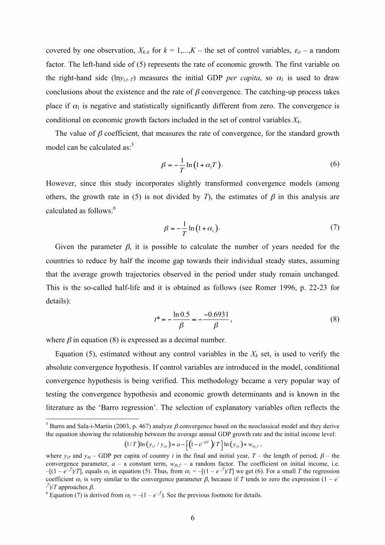
The value of β coefficient, that measures the rate of convergence, for the standard growth

model can be calculated as:5

. (6)

However, since this study incorporates slightly transformed convergence models (among

others, the growth rate in (5) is not divided by T), the estimates of β in this analysis are

calculated as follows:6

. (7)

Given the parameter β, it is possible to calculate the number of years needed for the

countries to reduce by half the income gap towards their individual steady states, assuming

that the average growth trajectories observed in the period under study remain unchanged.

This is the so-called half-life and it is obtained as follows (see Romer 1996, p. 22-23 for

details):

, (8)

where β in equation (8) is expressed as a decimal number.

Equation (5), estimated without any control variables in the Xk set, is used to verify the

absolute convergence hypothesis. If control variables are introduced in the model, conditional

convergence hypothesis is being verified. This methodology became a very popular way of

testing the convergence hypothesis and economic growth determinants and is known in the

literature as the ‘Barro regression’. The selection of explanatory variables often reflects the 5 Barro and Sala-i-Martin (2003, p. 467) analyze β convergence based on the neoclassical model and they derive the equation showing the relationship between the average annual GDP growth rate and the initial income level:

,

where yiT and yi0 – GDP per capita of country i in the final and initial year, T – the length of period, β – the convergence parameter, a – a constant term, wi0,T – a random factor. The coefficient on initial income, i.e. –[(1 – e–

βT)/T], equals α1 in equation (5). Thus, from α1 = –[(1 – e–

βT)/T] we get (6). For a small T the regression

coefficient α1 is very similar to the convergence parameter β, because if T tends to zero the expression (1 – e–

βT)/T approaches β.

6 Equation (7) is derived from α1 = –(1 – e–βT). See the previous footnote for details.

7

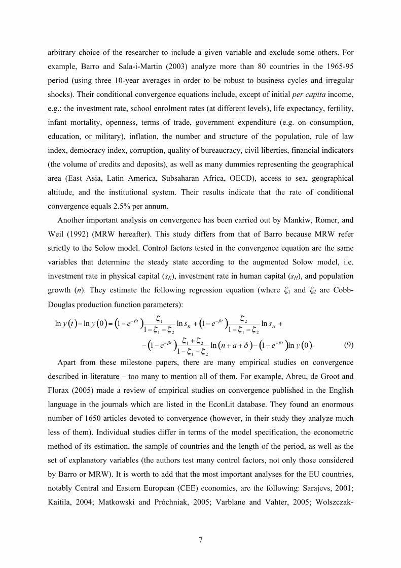
arbitrary choice of the researcher to include a given variable and exclude some others. For

example, Barro and Sala-i-Martin (2003) analyze more than 80 countries in the 1965-95

period (using three 10-year averages in order to be robust to business cycles and irregular

shocks). Their conditional convergence equations include, except of initial per capita income,

e.g.: the investment rate, school enrolment rates (at different levels), life expectancy, fertility,

infant mortality, openness, terms of trade, government expenditure (e.g. on consumption,

education, or military), inflation, the number and structure of the population, rule of law

index, democracy index, corruption, quality of bureaucracy, civil liberties, financial indicators

(the volume of credits and deposits), as well as many dummies representing the geographical

area (East Asia, Latin America, Subsaharan Africa, OECD), access to sea, geographical

altitude, and the institutional system. Their results indicate that the rate of conditional

convergence equals 2.5% per annum.

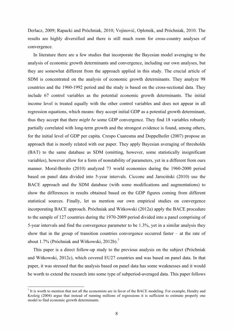
Another important analysis on convergence has been carried out by Mankiw, Romer, and

Weil (1992) (MRW hereafter). This study differs from that of Barro because MRW refer

strictly to the Solow model. Control factors tested in the convergence equation are the same

variables that determine the steady state according to the augmented Solow model, i.e.

investment rate in physical capital (sK), investment rate in human capital (sH), and population

growth (n). They estimate the following regression equation (where ζ1 and ζ2 are Cobb-

Douglas production function parameters):

. (9)

Apart from these milestone papers, there are many empirical studies on convergence

described in literature – too many to mention all of them. For example, Abreu, de Groot and

Florax (2005) made a review of empirical studies on convergence published in the English

language in the journals which are listed in the EconLit database. They found an enormous

number of 1650 articles devoted to convergence (however, in their study they analyze much

less of them). Individual studies differ in terms of the model specification, the econometric

method of its estimation, the sample of countries and the length of the period, as well as the

set of explanatory variables (the authors test many control factors, not only those considered

by Barro or MRW). It is worth to add that the most important analyses for the EU countries,

notably Central and Eastern European (CEE) economies, are the following: Sarajevs, 2001;

Kaitila, 2004; Matkowski and Próchniak, 2005; Varblane and Vahter, 2005; Wolszczak-

8

Derlacz, 2009; Rapacki and Próchniak, 2010; Vojinović, Oplotnik, and Próchniak, 2010. The

results are highly diversified and there is still much room for cross-country analyses of

convergence.

In literature there are a few studies that incorporate the Bayesian model averaging to the

analysis of economic growth determinants and convergence, including our own analyses, but

they are somewhat different from the approach applied in this study. The crucial article of

SDM is concentrated on the analysis of economic growth determinants. They analyze 98

countries and the 1960-1992 period and the study is based on the cross-sectional data. They

include 67 control variables as the potential economic growth determinants. The initial

income level is treated equally with the other control variables and does not appear in all

regression equations, which means: they accept initial GDP as a potential growth determinant,

thus they accept that there might be some GDP convergence. They find 18 variables robustly

partially correlated with long-term growth and the strongest evidence is found, among others,

for the initial level of GDP per capita. Crespo Cuaresma and Doppelhofer (2007) propose an

approach that is mostly related with our paper. They apply Bayesian averaging of thresholds

(BAT) to the same database as SDM (omitting, however, some statistically insignificant

variables), however allow for a form of nonstability of parameters, yet in a different from ours

manner. Moral-Benito (2010) analyzed 73 world economies during the 1960-2000 period

based on panel data divided into 5-year intervals. Ciccone and Jarociński (2010) use the

BACE approach and the SDM database (with some modifications and augmentations) to

show the differences in results obtained based on the GDP figures coming from different

statistical sources. Finally, let us mention our own empirical studies on convergence

incorporating BACE approach. Próchniak and Witkowski (2012a) apply the BACE procedure

to the sample of 127 countries during the 1970-2009 period divided into a panel comprising of

5-year intervals and find the convergence parameter to be 1.3%, yet in a similar analysis they

show that in the group of transition countries convergence occurred faster – at the rate of

about 1.7% (Próchniak and Witkowski, 2012b).7

This paper is a direct follow-up study to the previous analysis on the subject (Próchniak

and Witkowski, 2012c), which covered EU27 countries and was based on panel data. In that

paper, it was stressed that the analysis based on panel data has some weaknesses and it would

be worth to extend the research into some type of subperiod-averaged data. This paper follows

7 It is worth to mention that not all the economists are in favor of the BACE modeling. For example, Hendry and Krolzig (2004) argue that instead of running millions of regressions it is sufficient to estimate properly one model to find economic growth determinants.

9

that suggestion.

3. Methodology

A typical problem with growth regressions that comes up in most empirical econometric

research is related with the choice of proper form of the model, which can become

problematic even if well known theory of the considered phenomenon exists. Apart from the

typically econometric assumptions, it is usually far from obvious which of the possible

exogeneous variables should be included. For instance, Moral-Benito (2011) claims that there

are more than 140 variables proposed as growth factors in the mainstream of economic

growth literature yet analysis of the previous discussed research suggests that this figure is

underestimated. Certainly it is neither efficient nor sensible to include them all, even

assuming that a researcher has access to complete data. Usually though, incompleteness of the

data set theoretically allows for inclusion of a few dozens of independent variables. One way

of attaining growth empirics is to select those independent variables that reflect views of the

researcher on what the true model is. This, however is highly subjective, whereas different

preselected sets of independent variables can lead to totally different conclusions (as already

discussed in previous chapter), not to mention classical problems, such as a risk of omitted

variables bias. Another approach that has gained popularity over the last decade (though has

been present in literature in a quite agnostic form for two decades already) is to implement

some form of model averaging.

Let be a set of K variables considered as possible growth factors.

Further let be a set of C variables that according to our beliefs are growth

factors. Denoting GDP growth as Y, one can consider exactly 2K different linear growth

regressions such that in each there will be all elements of H and one of the 2K possible subsets

of X (including the empty one). The key question is: is there conditional GDP convergence

and which of the potential growth factors should be considered as the main ones. Let us

assume for the moment, that the model would be estimated with the use of cross-sectional

data, as in the paper by SDM (2004). We actually do believe that there is some conditional

GDP convergence in the considered groups of EU countries and thus we would include

lagged GDP level in H, whereas all the considered growth factors in X. In order to estimate

parameters reflecting the influence of particular Xk’s and Vm’s on the dependent variable,

denoted as without restricting attention to one model with selected

10

elements of X, BMA algorithm can be used. The idea of BACE, which if one of the BMA

algorithms used when a linear model is estimated via least squares method, is the following.

First, all the possible 2K above mentioned models denoted as M1,…,MJ (J being thus equal to

2K) are estimated. Also the subset of X used in Mj is denoted as Xj and the number of elements

in Mj as Kj. However, with even moderate K this is barely feasible due to extremely long time

required to estimate all the possible Mj’s. In that case, instead of estimating all 2K models that

can be constructed, a large number of Xj’s are drawn and models based on just the selected

subsets of X are estimated and further analyzed making J<2K. As it can be seen in empirical

research, this is a common practice (even the early birds, SDM do so, since their initial set of

independent variables contained over 60 variables) and it turns out that the estimators of

converge, thus in the discussed case one case use for estimating and

inference purposes just some drawn Mj’s instead of all the possible ones, provided that the

number of drawn Mj’s is large enough.

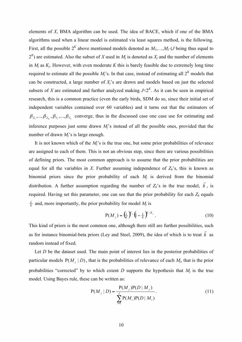
It is not known which of the Mj’s is the true one, but some prior probabilities of relevance

are assigned to each of them. This is not an obvious step, since there are various possibilities

of defining priors. The most common approach is to assume that the prior probabilities are

equal for all the variables in X. Further assuming independence of Zk’s, this is known as

binomial priors since the prior probability of each Mj is derived from the binomial

distribution. A further assumption regarding the number of Zk’s in the true model, , is

required. Having set this parameter, one can see that the prior probability for each Zk equals

and, more importantly, the prior probability for model Mj is

. (10)

This kind of priors is the most common one, although there still are further possibilities, such

as for instance binomial-beta priors (Ley and Steel, 2009), the idea of which is to treat as

random instead of fixed.

Let D be the dataset used. The main point of interest lies in the posterior probabilities of

particular models , that is the probabilities of relevance of each Mj, that is the prior

probabilities “corrected” by to which extent D supports the hypothesis that Mj is the true

model. Using Bayes rule, these can be written as:

. (11)

11

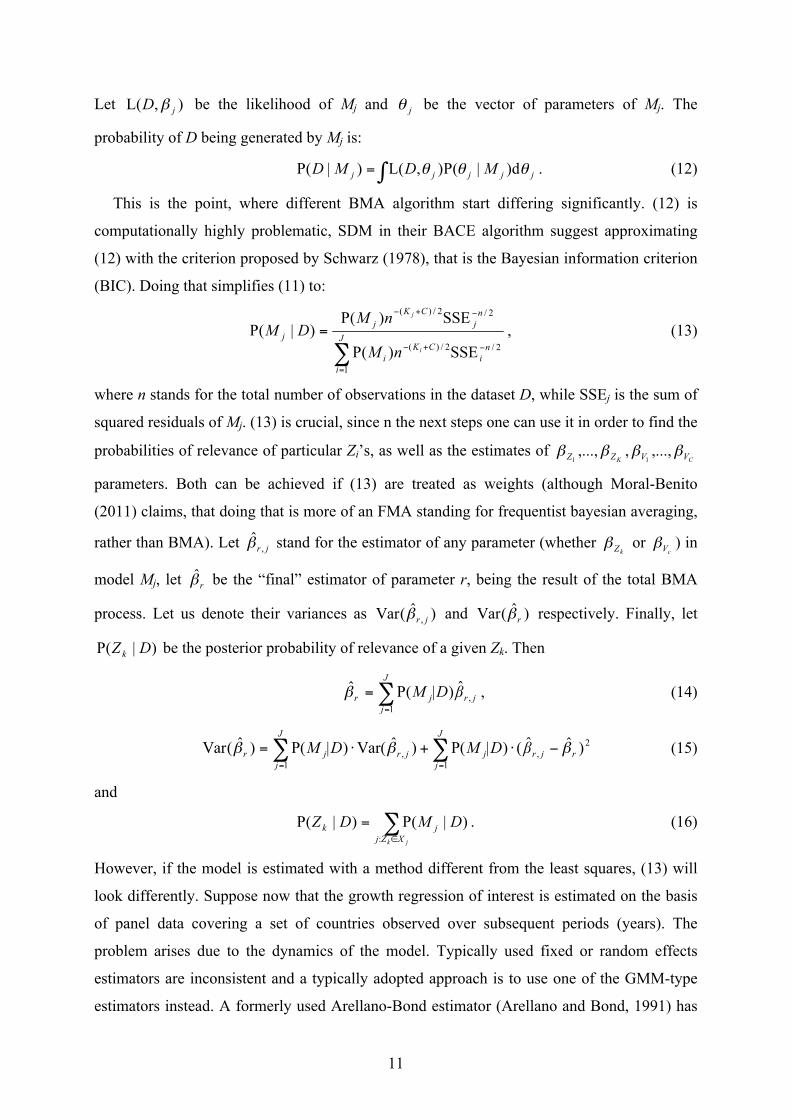
Let be the likelihood of Mj and be the vector of parameters of Mj. The

probability of D being generated by Mj is:

. (12)

This is the point, where different BMA algorithm start differing significantly. (12) is

computationally highly problematic, SDM in their BACE algorithm suggest approximating

(12) with the criterion proposed by Schwarz (1978), that is the Bayesian information criterion

(BIC). Doing that simplifies (11) to:

, (13)

where n stands for the total number of observations in the dataset D, while SSEj is the sum of

squared residuals of Mj. (13) is crucial, since n the next steps one can use it in order to find the

probabilities of relevance of particular Zi’s, as well as the estimates of

parameters. Both can be achieved if (13) are treated as weights (although Moral-Benito

(2011) claims, that doing that is more of an FMA standing for frequentist bayesian averaging,

rather than BMA). Let stand for the estimator of any parameter (whether or ) in

model Mj, let be the “final” estimator of parameter r, being the result of the total BMA

process. Let us denote their variances as and respectively. Finally, let

be the posterior probability of relevance of a given Zk. Then

, (14)

(15)

and

. (16)

However, if the model is estimated with a method different from the least squares, (13) will

look differently. Suppose now that the growth regression of interest is estimated on the basis

of panel data covering a set of countries observed over subsequent periods (years). The

problem arises due to the dynamics of the model. Typically used fixed or random effects

estimators are inconsistent and a typically adopted approach is to use one of the GMM-type

estimators instead. A formerly used Arellano-Bond estimator (Arellano and Bond, 1991) has

12

been widely criticized, among others due to its poor small sample properties, especially in

case of strong form of autoregression (Blundell et al., 2000), however other alternatives, such

as Blundell and Bond’s difference estimator exist (Blundell and Bond, 1998). It must be

emphasized that using GMM estimator is attractive not only due to poor statistical properties

of least squares estimators in the context of dynamic panel data models. Another equally

important feature is that applying least squares requires the assumption of strict exogeneity of

the independent variables, which in case of macroeconomic modeling is problematic, not to

say that practically cannot be fulfilled. This, however, can be overcome when instrumental

variables estimators are used, so it will thus be possible to relax the assumptions of

exogeneity, treating selected independent variables as endogeneous or predetermined.

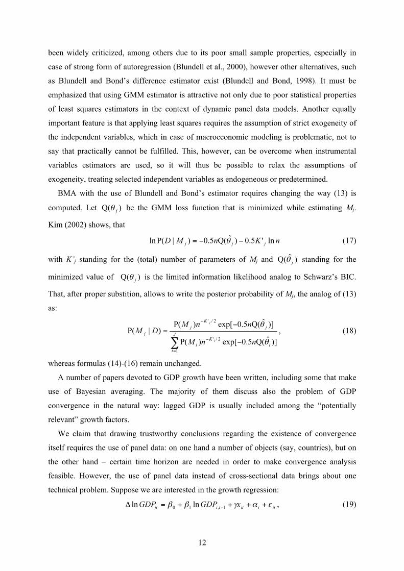
BMA with the use of Blundell and Bond’s estimator requires changing the way (13) is

computed. Let be the GMM loss function that is minimized while estimating Mj.

Kim (2002) shows, that

(17)

with K’j standing for the (total) number of parameters of Mj and standing for the

minimized value of is the limited information likelihood analog to Schwarz’s BIC.

That, after proper substition, allows to write the posterior probability of Mj, the analog of (13)

as:

, (18)

whereas formulas (14)-(16) remain unchanged.

A number of papers devoted to GDP growth have been written, including some that make

use of Bayesian averaging. The majority of them discuss also the problem of GDP

convergence in the natural way: lagged GDP is usually included among the “potentially

relevant” growth factors.

We claim that drawing trustworthy conclusions regarding the existence of convergence

itself requires the use of panel data: on one hand a number of objects (say, countries), but on

the other hand – certain time horizon are needed in order to make convergence analysis

feasible. However, the use of panel data instead of cross-sectional data brings about one

technical problem. Suppose we are interested in the growth regression:

, (19)

13

where is the logarithm of GDP change of i-th country in period t, is the

lagged by (usually) one period GDP level of i-th country, is the vector of growth factors

and control variables, is the individual effect of i-th country, , , are parameters of

the model and is the error term. It is clear that is endogeneous and it is also

quite problematic to apply instrumental variables methods so as to estimate the autoregressive

parameter. However, since , we can add to both

hand sides of (19), which results in

(20)

Naturally, is estimated as one parameter and obtaining the estimate of requires

simply subtracting 1 from the estimate of . It is relatively easy to propose some GMM

estimators that can be used to estimate , and in (20). As already mentioned, Blundell

and Bond’s estimator (Blundell and Bond, 1998), whose good statistical properties are

confirmed even in small samples is used in the article. Blundell and Bond’s approach requires

basically no serial correlation of the error term, its zero expected value conditional upon the

individual effects and the current values of the independent variables and, finally, additional

moment condition, namely:

(21)

for every country in the dataset (in the general formulation), stands for the change

of the dependent variable’s value from the first to the second period. Blundell and Bond’s

estimator and its particular properties shall not be discussed in great details here. The

interested reader can address the genuine paper. Still one thing worth mentioning about

Blundell and Bond’s estimator as applied in this paper is that it generally makes use of two

types of instruments: lagged levels and lagged changes of endogeneous and predetermined

variables (for the strictly exogeneous variables there is no need to use lags, since they do not

to be instrumentalized at all). In case of panel data sets that cover longer time period, that

means that the number of instruments can be huge. For instance, for the endogeneous

variables, their values lagged by at least two periods can be used. So, for the series of length

T=10, there are eight instruments for the 10th period. In most cases it is not a good idea to use

excessive number of instruments in such a case: it is time consuming and, first of all, raises a

risk of weak instruments problem in case that the autoregression of the considered

exogeneous variable is not very strong. It might seem trivial to mention the problem of slow

14

computation of a model estimated with numerous instruments. It must though be emphasized,

that running BMA requires estimation of at least thousands (if not millions) of models, so

long-lasting estimation process of each indeed plays a role. In order to reduce the risk of weak

instruments problem, as well as to save time, the number of instruments used is reduced: for

each endogeneous and predetermined variable, no more than its two lags and levels are used

as instruments.

Another problem related with many economic models, including (20), is the possible lack

of stability. Writing the model in such a way also means assuming that , and are

constant overtime, which we generally doubt. Naturally, if a truly short period of time is

considered, this assumption sounds rational. Nevertheless, with longer time horizon it will

almost surely not hold, especially if some crucial moments are “on the way”. For instance, if

we were to consider a group of Central and Eastern European (CEE) countries in the period

that covers late 80’s or early 90’s of the twentieth century (like, for example, Próchniak and

Witkowski, 2012b), it would be rational to allow for structural break somewhere around the

1990. Certainly in case of some of the independent variables the assuming stability of the way

they influence is rational, still for some of them – it is not anymore. We claim that it

would thus be useful to take potential structural break into consideration.

Crespo Cuaresma and Doppelhofer (2007) consider the case of differing regimes overtime.

In their model they introduce a set of variables that are potentially causing “threshold

nonlinearity”. The name “nonlinearity” comes from the fact that the variables that change the

regime overtime are introduced by means of interaction terms, which, being a product of

variables, can indeed be viewed as nonlinear.

In the model nonstability of the relation between the dependent and the independent

variables is introduced in a manner that is partly similar to Crespo Cuaresma and Doppelhofer

(2007). First, the set of considered independent variables is divided into two groups: those

that are assumed to have stable effect on the dependent variables and those whose effect can

vary overtime. We use our economic beliefs for that preselection, which might be subjective

though. In the next step the entire period covered by the considered panel is divided into a few

subperiods and assume that the way that all independent variables affect the dependent

variable is constant for a given subperiod, but might differ in different subperiods for the

variables selected in the previous step. Then “regime” variables: R1, R2, …, with

standing for the number of subperiods the entire series have been divided into are introduced.

Each , standing for the value of “R” variable for u-th subperiod (u=1,…,U), takes on a

15

value of 1 for such observation on the i-th object (country) in period t, that t is covered by the

u-th subperiod and 0 otherwise. Let Vc be a variable whose influence on the dependent

variable can be different in particular subperiods. In order to test for the stability of this

influence, it is possible to follow one of two equivalent procedures. The first option is to

include in H a set of independent variables that are products of Vc and particular ’s,

u=1,…,U, that is: ={ }. In order to check for stability of the influence

of the considered Vc on the dependent variable, one would need to check for significance of

differences in the parameters on such set of products, that can be viewed as interaction terms

of Vc and ’s. Another possibility is to introduce into the model the Vc and the products of

Vc with any U-1 of the U ’s, that is, for instance, ={ }. In this

case checking for the discussed stability would consist in checking for significance of the

set itself.

The above mentioned strategies might not be equivalent for the set

anymore. The problem lies in the way particular Zk’s are drawn for particular Mj’s in

subsequent replications of BMA algorithm. Two strategies are possible here. One of them is

to draw groups of variables rather than variables themselves. Suppose we believe the

influence of a given Zk on the dependent variables varies overtime. In such a case we add

interaction terms of the Zk and particular Ru’s to the X set. “Drawing groups” means that if Zk

is drawn as a part of Xj for a given Mj, then we automatically add all its interactions to Xj as

well. The second strategy would consist in treating interactions of Zk and particular Ru’s as

separate variables being a part of X. The advantage of the first strategy is that fewer

replications of BMA are needed and that it seems slightly more logical. However, the

posterior probabilities computed in BMA would not be calculated separately for each of the

interactions – those would be found for the entire group. One would thus not be able to use

Bayesian posterior probabilities in order to conclude whether it is just the Zk that influences

the dependent variable in some, constant overtime, way, or maybe is the influence of the Zk

different in particular subperiods. The second drawing strategy seems better in this respect:

posterior probabilities are found for each interaction term separately and we can thus conclude

that, for instance, there is Bayesian confirmation of the influence of Zk on the dependent

variable, but there is no confirmation of such an influence’s variability overtime.

The second drawing strategy is thus adopted, that is draw separate variables, interaction

terms included, rather than groups. Similarly as in the case of H set, for a variable with

16

potentially unstable influence on the dependent variable overtime we can include either

={ } or ={ } in X. However with the

second (individual) drawing strategy on our minds we think it is better to include rather

than in X. There rationale behind that is the following. Suppose we use as a part of

X. In the case of a model with all elements of included, the last subperiod (the one for

which no interaction term of Zk and Ru has been introduced) becomes a reference subperiod.

The parameter estimated on Zk reflects then only the influence of Zk on the dependent variable

in the reference subperiod, whereas the parameter on each interaction term of Zk and a given

Ru reflects the difference between the influence of Zk on the dependent variable in period u

and the reference period. However, in an Mj in which the only element included from is

the Zk itself, the parameter on Zk reflects its influence on the dependent variable in the entire

period covered by the dataset. That means that the meaning of the parameter on Zk differs in

particular models, which certainly is the effect one would like avoid. Still this problem does

not appear if is included in X and that is why that solution is applied. As already

mentioned, in case of Vc variables, whether or are used, the above discussed

problem does not exist since the whole set H is included in every Mj, thus we can also use

if convenient.

4. Data

The variables included in the analysis are listed in Table 1. 22 growth factors are tested as

control variables reflecting the differences in steady states. This group encompasses both

‘direct’ factors, which have an immediate impact on economic growth from the demand-side

and supply-side perspective, as well as ‘deep’ growth determinants, representing the

countries’ institutional environment.

The variables included into the set of control factors are divided into three subgroups:

endogenous variables, predetermined variables, and exogenous variables. Such a division

should be made due to the chosen method of model estimation. In the case of OLS regression,

all the variables are assumed to be exogenous. However, Blundell and Bond’s GMM system

estimator requires that the variables be divided into three mentioned subgroups. The division

is made on the basis of the economic theory but, to some extent, it reflects our own opinions

and there is some room for an arbitrary choice. First of all, all the variables that are associated

17

with monetary and fiscal policies are treated as endogenous. This reflects the fact that they are

likely to be mutually correlated with GDP. Economic policy affects of course the rate of

economic growth but the actions taken by the government and the central bank depend also on

the current rate of economic development. For example, on the one hand, a decrease in

interest rate accelerates economic growth, but – on the other hand – fast economic growth and

inflationary pressures often lead the central bank to raise interest rates. There is also empirical

evidence that government expenditure both determine and are influenced by the level of GDP.

Similarly, inflation may be the result of rapid economic growth but it may be also detrimental

to further output expansion.

Moreover, all the variables that are related with components of aggregate demand are also

classified as endogenous. For example, investments and the openness rate are treated as

endogenous variables because rapid economic development enhances to invest (especially by

foreign companies, but also by domestic entities), as well as it determines the level of imports

which is included in the openness ratio. The endogeneity of the variables related with human

capital reflects the fact that slow economic growth does not allow to rapid accumulation of

human capital. If the economy develops slowly, few resources are devoted for human capital

accumulation (e.g. there are low expenditures on R&D and education). Finally, services are

the most productive sector and they much contribute to economic growth, but – on the other

hand – rapid economic growth in the case of countries under study (EU members) occurs

basically by the expansion of the service sector.

The set of predetermined variables includes two qualitative indices referring to deep

economic growth determinants that measure the countries’ institutional environment. These

include index of economic freedom and democracy index. The main idea of classifying index

of economic freedom as the predetermined variable is the fact that it is a qualitative index

compiled of a number of category indices and many of these category indices represent the

country’s macroeconomic performance observed in the earlier years. Since democracy index

also represents deep economic growth determinants and it is similarly constructed, it is

reasonable to include both variables into the same category.

The last category (exogenous) includes all the remaining variables.

All the calculations are carried out on the two types of data: figures transformed into three-

year subperiods and annual time series of the variables involved, the latter ones being typical

panel data. Each of these methods of data transformation has its own strengths and

weaknesses. In this paper, the results obtained based on 3-year intervals are treated as

benchmark findings and are primarily discussed.

18

The main benefit of including annual panel data is a large number of observations, which

increases the statistical significance of the estimated model. However, annual data are biased

because they are largely influenced by business cycles and irregular movements; the latter

ones being the result of various supply-side and demand-side shocks, both internal and

external (the good example is the recent global crisis). For that reason in empirical studies on

economic growth the cross-sectional approach is widely used by averaging the time series for

the whole period or for several subperiods (encompassing typically 3-, 5-, or 10-year

intervals). Such an approach allows the researcher to smooth the time series and analyze the

medium-term and long-term relationships between the variables involved, getting rid of the

short-term fluctuations. The longer are the subperiods for which the data are averaged, the

smoother are the variables and the longer-term relationships between them are evidenced.

However, when averaging the data, the number of observations falls dramatically leading to a

reduction of statistical significance of the results. Hence, this study incorporates 3-year time

intervals to achieve a reasonable compromise between the statistical and economic

significance. Thus, the subperiod-averaged calculations for the EU27 countries are based on

the following subperiods: 1993-1995, 1996-1998, 1999-2001, 2002-2004, 2005-2007 and

2008-2010, while those for the EU15 countries include also the subperiods: 1972-1974, 1975-

1977, 1978-1980, 1981-1983, 1984-1986, 1987-1989, 1990-1992.

The results for the annual panel data and 3-year intervals constitute a type of robustness

check and need not be the same. Moreover, they may be entirely different because of the

factors mentioned above (annual data and 3-year averaged data document different

relationships: short-term and medium-term respectively, so the outcomes may vary).

The study is based on a partly balanced panel. This means that, if a given observation is

included, there are no missing values of any of the explanatory variables. However, the panel

is not fully balanced because for some countries there are missing observations for some

years. However, such a partly balanced panel is correct for the applied methodology because

it requires that all the calculations are based exactly on the same observations. So if a given

observation is included, it appears in all the regression models.

Since this study focuses on the time stability of parameters measuring the impact of

particular variables on economic growth, many variables are included into the model with

interactions. Table 1 shows the types of interactions and lists the variables for which the time

stability of parameters is being verified.

First of all, the time stability of the convergence parameter is analyzed. That is why the

variable measuring the initial GDP per capita level is included with interactions. Since the

19

initial income level appears in all the estimated models, it is characterized by interactions of

the type (the lagged GDP per capita is the only variable included in the H set). Second,

the interactions are also present in the case of all the variables representing monetary and

fiscal policy. It is assumed that the impact of economic policy on GDP dynamics is not

constant over time. It depends on many factors, including the internal and external sources,

and it might vary between the 1970s, 1980s, 1990s, and 2000s. The economic and political

situation in the world is changing continuously and there are no reasons to believe that the

impact of economic policy on GDP growth is constant. For example, during the

contractionary periods fiscal and monetary tightening could have completely different effects

as compared with the expansionary periods. That is why structural breaks in all these

variables are allowed. Finally, interactions are introduced for the investment rate and the

openness ratio to check whether they exhibited varying impact on the rate of economic

growth. All the explanatory variables except lagged GDP for which varying impact on

economic growth is assumed are included into the model with the type of interactions.

Before carrying out the analysis, the expected dates of structural breaks should be

introduced into the model. In the case of EU27 countries, the existence of the two structural

breaks is assumed. The first turning point takes place in 1998, being related with two things.

First, it lies exactly in half-life between the end of transformation recession in most of the

CEE countries and the year of the first EU enlargement. This could show whether the impact

of particular variables changed between the period that was much more affected by the

transformation from a centrally-planned to market-based system (i.e. the years 1993-1998)

and the period that was rather influenced by preparations to EU enlargement (1999-2004). In

the early years of transition, economic growth paths of the CEE countries were less influenced

by the EU policies, encompassing EU structural and aid funds. An additional factor to choose

the year 1998 as the structural break is the Russian crisis. In 1998, GDP in Russia fell by

more than 5% that might affect many of the countries under study because of their very strong

links with Russia. The second structural break is assumed to be in 2004. The choice of this

year is rather obvious – it is the time of the first EU enlargement. EU enlargement could

significantly affect the relationships between the macroeconomic variables of the EU

countries. Since the time series are available till 2010, the model cannot include the third

structural break in 2007, that is when Bulgaria and Romania joined the EU, because the time

spans would be very short and the results would not be reliable.

In the case of EU15 countries, for which the available time series are longer, the third

20

structural break in 1989 has been introduced (which is de facto the earliest turning point). The

choice of this year results from the fact that it is considered as the end of the socialist era in

most of the transition countries. In 1989, market economies emerged in Central and Eastern

Europe and there are reasonable expectations that the mechanisms driven the development of

EU15 countries could change significantly in that year. The remaining two turning points

(1998 and 2004) are introduced also in the case of EU15 countries.

5. The results of the analysis

The results of the analysis are illustrated in Tables 2-6. The presentation and interpretation of

the outcomes are primarily focused on the 3-year intervals. In some areas, however, these

results are compared with those for panel data.

(a) Convergence

The reference period for the lagged GDP variable is the 2005-2010 subperiod. For these

years, the estimated coefficient on initial GDP equals 0.8412 for the EU27 countries and 3-

year intervals. Since the latter figure is not the typical coefficient on initial income in the

convergence model because the explained variable is the GDP level and not the growth rate,

the estimated coefficient standing for initial income in the untransformed convergence

regression where the growth rate of GDP is the explained variable and the GDP from the

previous year is the explanatory variable should be obtained by subtracting one from that

value. Hence, for the 2005-2010 period it equals: 0.8412 – 1 = –0.1588. The pseudo t

statistics amounts to 30.02 meaning that, given reasonable significance levels, the estimated

coefficient is statistically significantly different from zero. These results indicate the existence

of β-convergence among the EU27 countries during the 2005-2010 period. This informs that

the average 3-year growth rate of GDP was negatively related with the initial income level. Of

course, the convergence is conditional on the growth factors included in the analysis. It is

assumed that the countries do not tend to one common hypothetical steady-state, but to

different steady-states determined by the explanatory variables (see Table 1 for the list of

them). Given the estimated coefficient on initial income, it is possible to calculate the β-

convergence parameter. Applying formula (7) by substituting –0.1588 for α1 and 3 for T (i.e.

the length of one subperiod in terms of number of years), yields β = 5.77%.

21

How do these results differ from those for the other distinguished subperiods? For the

EU27 countries and the 3-year averages it turns out that there are no statistically significant

differences in the pace of the convergence process between the respective subperiods. The β-

convergence parameter for the first subperiod encompassing the years 1993-1998 equals

5.91% and the corresponding estimated coefficient on initial income in the untransformed

regression equation amounts to –0.1625 (to calculate the latter figure, the estimated

coefficient on lagged GDP for the reference subperiod (2005-2010) should be added to that on

lagged GDP in interaction with the first subperiod (1993-1998), subtracting one from the

total). As we can see, during the years 1993-1998 the convergence process occurred

somewhat more rapidly than in 2005-2010; however, the pseudo t statistics for the lagged

GDP in interaction with the first subperiod equals –1.44 being less than 2 in absolute terms.

This means that the estimated coefficient on initial income for the years 1993-1998 was not

statistically significantly different than that for 2005-2010 demonstrating that the convergence

process of the EU27 countries in the 1993-1998 period was not statistically faster (assuming

reasonable significance levels) than in the 2005-2010 period.

The parameter β for the 1999-2004 subperiod is calculated by following the same steps as

before. The estimated coefficient standing on lagged GDP in interaction with the second

subperiod equals 0.0015 implying that the estimated coefficient on initial income in the

untransformed convergence regression amounts to –0.1573 and β = 5.71%. Like before, the

pseudo t statistics for the estimated coefficient on lagged GDP in interaction with the second

subperiod equals 0.77 pointing to no statistically significant difference.

These results based on the 3-year intervals are quite similar to those for the panel data and

the EU27 countries. Using information presented in Table 4, it is possible to calculate the

estimates of β for all the subperiods (based again on equation (7), but substituting 1 for T as

panel data are annual time series). The betas for the EU27 countries are equal to 5.18%,

4.99%, and 5.27% respectively for the subperiods 1993-1998, 1999-2004, and 2005-2010.

Like in the case of 3-year intervals, the estimates of this coefficient are not highly

differentiated but, unlike the previous case, the β parameter for the 1999-2004 subperiod is

statistically significantly different than that for the reference 2005-2010 subperiod (although

from the economic point of view this difference is not very large).

Based on the above results, it is possible to formulate the first three findings of the

research. First, the analysis indicates a very rapid pace of β-convergence process among the

EU27 countries as compared with many other studies. The applied methodology, namely

22

Blundell and Bond’s GMM system estimator, better extracts the pure convergence rate as

compared with the other studies incorporating standard econometric techniques. Moreover,

since the Bayesian model averaging is used, this result is not spurious that would be so in the

case of estimating only one model with the arbitrary (and to some extent random) choice of

explanatory variables. Millions of regressions have been estimated here and the convergence

rate of about 5-6% seems to reveal a true relationship between the initial income level and the

subsequent growth rate.

Second, it turns out that the speed of convergence among the EU27 countries did not differ

much between the respective subperiods. The benchmark subperiod includes the years 2005-

2010 for which the β-coefficient equals 5.77% in the case of 3-year intervals and 5.27% in the

case of panel data. For the earlier subperiods the betas amount to 5.91% or 5.18% during

1993-1998 and 5.71% or 4.99% during 1999-2004. They are mostly statistically indifferent

than those for the reference subperiod.

Third, the analysis based on 3-year intervals makes it possible to better extract the true

relationship between the initial income level and the growth rate. That is why the estimates of

β based on the 3-year intervals are slightly higher.

Given the value of the β-convergence parameter, it is possible to estimate the number of

years the countries need to reduce by half their distance towards the steady state (assuming of

course that steady-states differ only in terms of the control variables included in the model).

Applying equation (8), the half-lives are about 12-14 years for the EU27 countries (see Table

6 for details).

Despite the above differences between the pace of convergence in the respective

subperiods, this analysis points to an evidently higher average pace of convergence as

compared with the majority of the other empirical studies. According to these results, Central

and Eastern European countries converged to Western Europe at the average rate of 5-6% per

annum. Such a pace of convergence is by no doubt a novum given the existing mainstream of

knowledge, but of course some authors have already found that such results may appear. As it

has been shown in the review of the literature, the pace of convergence commonly known as

the worldwide pace of convergence is about 2% per year. Of course, the individual studies

differ in this respect, often pointing to lower or higher convergence parameters. For example,

some of the studies focused on the transition countries, notably the CEE economies, indicated

more rapid pace of convergence. Similarly, Abreu, de Groot and Florax (2005), who analyzed

619 convergence models taken from 48 different studies, argue that the average convergence

coefficient calculated based on these models equals indeed about 2%, but according to them it

23

is not proper to say about a 2% natural convergence rate because various convergence models

are estimated based on different samples. For example, the models based on the Solow

formula and those which account for differences in fiscal policy and financial sector

development yield the estimates of the convergence coefficient largely exceeding a legendary

2% level. Moreover, their literature review also suggests that when estimators such as LSDV

or GMM are used, which allow to account for the specific effects of the individual countries,

the estimated convergence coefficients are also significantly higher. These results confirm

those views of significantly higher convergence coefficients than a legendary 2% level;

moreover these results are robust to the choice of explanatory variables so they show a true

and stable relationship.

In a similar way, it is possible to calculate the convergence parameters for the EU15

countries. Those are equal to about 3% both for 3-year intervals and for panel data. Table 6

gives the details. In the case of EU15 countries, the estimated coefficients based on panel data

are statistically significantly different between the respective subperiods, but the calculations

made on the 3-year intervals do not confirm it. These results imply that the group of Western

European countries converges slower than the whole group of the enlarged EU. It is thus

possible to infer that the convergence among the EU27 countries is mainly driven by the

convergence of CEE towards EU15. Indeed, looking at the official statistics, the CEE

countries recorded more rapid economic growth rates than the EU15 economies while the

GDP of the former ones used to be much lower.

The results of this analysis in terms of conditional β-convergence are more reliable than

those evidenced by the other authors due to several reasons. First, the Bayesian averaging of

estimates is a method of data analysis which is not biased by an arbitrary choice of the

variables that are included in the regression equation. In fact, these results are free of this

selection bias (except, of course, some initial preselection of the time series). A huge number

of regression equations is estimated, each of them being based on a different set of variables

chosen from the preliminary dataset. Such a method of analysis is not included in any of the

studies except those that incorporate Bayesian averaging of estimates. Second, unlike in many

other studies based on Bayesian modeling, this paper applies Blundell and Bond’s GMM

system estimator which is a more advanced and better tool to verify the research hypotheses

(but some weaknesses of this methodology, like any other research method, still persist). Most

authors who incorporate the Bayesian approach use the Bayesian averaging of classical

estimates and estimate the growth regressions using standard OLS estimators. In this study,

however, Blundell and Bond’s GMM system estimator is used to extract the true value of the

24

β-convergence coefficient. Third, unlike in all the studies conducted by the other authors and

cited in the literature review, the initial income level is the variable which is included here in

all the regression equations. The initial GDP per capita level is thus treated differently than

the other economic growth determinants; the latter ones may appear in a given regression

equation or not meanwhile the initial GDP per capita level always is included as one of the

explanatory variables. As the result, this methodology seems to be better for estimating the

true value of the convergence parameter.

The conditional β convergence coefficients are relatively high indicating quite rapid

achievement of the individual steady states. It means that there are huge differences in

marginal products of the inputs in the countries under study. The countries that are poorer

record much higher factor productivity and achieve more rapid economic growth (in

conditional terms) than those that are richer. However, this also means that gains from being

poorer may be exhausted quite soon and increasing GDP due to the pure convergence process

is limited.

(b) Economic growth determinants

The results on economic growth determinants are quite differentiated between both groups

of countries and both types of models. The details are presented in Tables 2-5. Here, the most

important implications are described with some interpretation and explanation of the

outcomes.

The interest rate is one of the most important variables determined by the central bank. Its

impact on the rate of economic growth was negative in the case of EU27 countries and 3-year

intervals. This is in line with the economic theory and the basic macroeconomic models. As

the investment function suggests there is a negative relationship between investment and

interest rate. Because investment is part of GDP, this negative relationship exists also between

interest rate and GDP. Thus, high interest rate negatively affects investment (as well as net

exports if included into the model), decelerating the pace of economic growth. However, in

some cases the positive relationship between interest rate and economic growth has been

evidenced, especially for the last distinguished subperiods (both for the EU15 and EU27

countries). There is, of course, no one unambiguous explanation of this outcome but it may be

expected that this positive relationship between interest rate and economic growth is

somewhat related with the global economic and financial crisis and very disturbing situation

observed in the analyzed countries in the last years. Interest rates were very low recently.

25

Central banks were decreasing interest rates to boost the economy. However, these actions did

not succeed in many cases and despite a fall in interest rates the rate of economic growth did

not accelerate.

Inflation is a variable that often behaves very similar to interest rates. For example,

according to the Fischer hypothesis, the fluctuations in interest rates reflect the fluctuations in

inflation. Partly due to this fact, but also because of some other causes, the results for inflation

are similar to those for interest rate. For the EU27 countries and 3-year intervals, a negative

impact of inflation on economic growth has been evidenced for all the considered subperiods.

This is in line with the classical model according to which inflation is countercyclical and it is

by no way a factor conducive to economic growth. However, in the case of panel data and the

last subperiods, a positive relationship between inflation and GDP dynamics was recorded.

This can be explained twofold. First, panel time series reflect short-run links between the

variables involved and in the short run the economy is likely to behave according to the

Keynesian or demand-side approach according to which economic growth may exist with

some inflation. Second, in the last subperiod, that is during 2005-2010, inflation rates among

the EU members were low (two-digit inflations occurred extremely rarely while some

countries in these years suffered even deflation). In such circumstances, low inflation (or even

deflation) need not be a factor conducive to rapid economic growth and that is why a positive

sign of the parameter has been obtained.

The results for the annual change of the domestic credit are generally in line with the

economic theory but some exceptions are present. The positive relationship between this

variable and economic growth has been mostly obtained confirming the theoretical structural

model according to which financial sector development is conducive to economic growth.

However, one has to take into account that excessive lending might be dangerous to economic

development, especially nowadays when the level of both private and especially public

indebtedness of many EU countries is enormous. Many countries suffer from high costs of

repaying loans and their level of debt hampers the growth of GDP. It is hardly to expect that

such a relationship is confirmed by this model but the results for some subperiods do not point

to a clear-cut positive relationship between credit growth and economic growth. The most

statistically significantly negative relationship was recorded by the panel data for the EU27

countries and the 2005-2010 subperiod. This may be caused by the fact that the Baltic states’

growth of GDP was mainly based on credit and partly because of it the Baltics suffered the

biggest recession in 2009; some of these countries noted also the fall of GDP in 2008 and/or

2010.

26

Surprisingly, the study does not indicate a clear-cut positive impact of investment (saving)

on economic growth both in the case of EU15 and EU27 countries as well as in the case of

panel and 3-year data. It may be thus expected that investments in Central and Eastern as well

as Western Europe relatively often flowed into unproductive activities. In other words,

investment outlays were not so productive to affect significantly the rate of economic growth

(some other variables turned out to be more significant). This result emphasizes the need for

the revision of some government programs promoting both investments and savings.

The model demonstrates that government expenditures on consumption are

counterproductive. Negative and statistically significantly different than zero estimated

coefficients standing for government consumption have been obtained in most considered

subperiods regardless the group of countries (EU15 or EU27) and the way of data

transformation. Hence, to accelerate economic growth, the authorities should put emphasis on

the reduction of public unproductive spending. Indeed, what matters first of all is public

investment and not public consumption. Fiscal expansion by stimulating government

consumption is counterproductive although it is very popular from the social point of view

because such expenditures are related with a direct and immediate transfer of money from

government to households and firms. However, this study clearly confirms that such results

are not conducive to output growth.

The results for the openness rate (the ratio of exports plus imports to GDP) do not point to

a stable positive or negative impact on economic growth. They vary considerably between the

consecutive subperiods. This is likely caused by the fact that this variable is rather related

with the size of a given country (small countries tend to have much more open economies) as

well as with the fact that this variable may reveal long-term impact on economic growth,

which is not well evidenced in this study.

Finally, the analysis includes a number of other economic growth determinants which enter

regression equations without interactions. The most important findings for the EU27 countries

and the 3-year intervals are the following.

First, the most significant variable in this group is the index of economic freedom.

Moreover, the estimated coefficient for the index of economic freedom is positive and

statistically significantly different than zero in all the four variants of the model. This

indicates a clear-cut and strong positive relationship between the scope of economic freedom

and output growth. Economic freedom is a variable that can be treated as a proxy for the

country’s institutional environment. As it has been already said, institutions are ‘deep’

economic growth determinants. This research confirms an important role of some types of

27

institutions in stimulating economic growth. However, another institutional variable, namely

the democracy index, turns out to be statistically significant only for the EU27 countries and

3-year intervals but for the other three considered models the estimated coefficient is

statistically insignificant. The latter result may be caused by the fact that there is some

empirical evidence suggesting that democracy often reveals a nonlinear relationship with

economic growth (a strong nondemocratic environment may contribute to GDP in the same

way as a very democratic one).

Second, the analysis suggests an important role of foreign direct investment in stimulating

economic growth. This outcome has direct policy implications because it indicates that the

authorities should conduct actions to enhance foreign investments. The gains from FDI has

not been exhausted yet and there is still much room to undertake investment projects which

are productive from the point of view of the whole economy.

Third, as regards human capital, the results are mixed. This surprising outcome does not of

course mean that human capital has a negative impact on economic growth. It rather means

that the variables included are not as good for empirical studies on economic growth as one

might initially expect and there is still much room for carrying out empirical and theoretical

analyses aiming at finding the best proxies for human capital stock. Moreover, human capital

determines the volume of output from the supply-side perspective, that is rather in the long

run, which is not well evidenced by the calculations performed in this study.

6. Conclusions

The analysis yields a number of interesting findings on the nature of economic growth in the

EU member states. (1) The EU27 countries converged at the rate of about 5-6% per annum

while the EU15 countries – at about 3% per year. Both these figures constitute an enormous

difference as compared with the widely cited 2% speed of convergence. (2) The pure

mechanism of conditional convergence of the countries under study was rather constant over

time: there were periods of more rapid or slower convergence but the differences were not so

huge as initially expected. (3) The considered economic growth determinants exhibited very

mixed and differentiated impact on economic growth in various subperiods; a part of this

instability was undoubtedly caused by the global and financial crisis as well as by the

economic problems arising in many EU countries in the last years. (4) The subperiod-

averaged data allow for better extraction of the pure rate of conditional convergence than the

panel data.

28

References

Abreu M., de Groot H., Florax R. (2005), A Meta-Analysis of β-Convergence: The Legendary

2%, Journal of Economic Surveys, 19, pp. 389-420.

Arellano M., Bond S. (1991), Some Tests of Specification for Panel Data: Monte Carlo

Evidence and an Application to Employment Equations, Review of Economic Studies, 58,

pp. 277-297.

Barro R.J. (1991), Economic Growth in a Cross Section of Countries, Quarterly Journal of

Economics, 106, pp. 407-443.

Barro R.J., Lee J.-W. (1994), Sources of Economic Growth, Carnegie-Rochester Conference

Series on Public Policy, 40, pp. 1-46.

Barro R.J., Sala-i-Martin X. (2003), Economic Growth, The MIT Press, Cambridge - London.

Blundell R., Bond S. (1998), Initial Conditions and Moment Restrictions in Dynamic Panel

Data Models, Journal of Econometrics, 87, pp. 115-143.

Blundell R., Bond S., Windmeijer W. (2000), Estimation in Dynamic Panel Data Models:

Improving on the Performance of the Standard GMM Estimator, in: B. Baltagi (ed.),

Nonstationary Panels, Panel Cointegration and Dynamic Panels, Elsevier Science.

Ciccone A., Jarociński M. (2010), Determinants of Economic Growth: Will Data Tell?,

American Economic Journal: Macroeconomics, 2, pp. 223-247.

Crespo-Cuaresma J., Doppelhofer G. (2007), Nonlinearities in Cross-Country Growth

Regressions: A Bayesian Averaging of Thresholds (BAT) Approach, Journal of

Macroeconomics, 29, pp. 541-554.

Hendry D.F., Krolzig H.-M. (2004), We Ran One Regression, Oxford Bulletin of Economics

and Statistics, 66, pp. 799-810.

Islam N. (2003), What Have We Learnt from the Convergence Debate?, Journal of Economic

Surveys, 17, pp. 309-362.

Kaitila V. (2004), Convergence of Real GDP Per Capita in the EU15. How Do the Accession

Countries Fit In?, Working Paper No. 25, ENEPRI, Brussels.

Kim J.-Y. (2002), Limited Information Likelihood and Bayesian Analysis, Journal of

Econometrics, 107, pp. 175-193.

Ley E., Steel M. (2009), On the Effect of Prior Assumptions in Bayesian Model Averaging

with Applications to Growth Regression, Journal of Applied Econometrics, 24, pp. 651-

674.

29

Mankiw N.G., Romer D., Weil D.N. (1992), A Contribution to the Empirics of Economic

Growth, Quarterly Journal of Economics, 107, pp. 407-437.

Matkowski Z., Próchniak M. (2005), Zbieżność rozwoju gospodarczego w krajach Europy

Środkowo-Wschodniej w stosunku do Unii Europejskiej, Ekonomista, 3, pp. 293-320.

Moral-Benito E. (2010), Determinants of Economic Growth: A Bayesian Panel-Data

Approach, Working Paper No. 719, CEMFI, Madrid.

Moral-Benito E. (2011), Model Averaging in Economics, Working Paper, Bank of Spain.

Próchniak M., Witkowski B. (2012a), Konwergencja gospodarcza typu β w świetle

bayesowskiego uśredniania oszacowań, Bank i Kredyt, 43, pp. 25-58.

Próchniak M., Witkowski B. (2012b), Real β Convergence of Transition Countries – Robust

Approach, Eastern European Economics (in print).

Próchniak M., Witkowski B. (2012c), Bayesian Model Averaging in Modelling GDP

Convergence with the Use of Panel Data, Roczniki Kolegium Analiz Ekonomicznych

SGH (in print).

Rapacki R., ed. (2009), Wzrost gospodarczy w krajach transformacji: konwergencja czy

dywergencja?, PWE, Warszawa.

Rapacki R., Próchniak M. (2010), Economic Growth Paths in the CEE Countries and in

Selected Emerging Economies, 1993-2007, Research in Economics and Business: Central

and Eastern Europe, 2, pp. 5-33.

Romer D. (1996), Advanced Macroeconomics, McGraw-Hill, New York.

Sala-i-Martin X. (1996a), Regional Cohesion: Evidence and Theories of Regional Growth and

Convergence, European Economic Review, 40, pp. 1325-1352.

Sala-i-Martin X. (1996b), The Classical Approach to Convergence Analysis, Economic

Journal, 106, pp. 1019-1036.

Sala-i-Martin X., Doppelhofer G., Miller R. (2004), Determinants of Long-Term Growth: A

Bayesian Averaging of Classical Estimates (BACE) Approach, American Economic

Review, 94, pp. 813-835.

Sarajevs V. (2001), Convergence of European Transition Economies and the EU: What Do

the Data Show, Discussion Paper No. 13, BOFIT, Helsinki.

Schwarz G. (1978), Estimating the Dimensions of a Model, Annals of Statistics, 6, pp. 461-

464.

Solow R.M. (1956), A Contribution to the Theory of Economic Growth, Quarterly Journal of

Economics, 70, pp. 65-94.

30

Varblane U., Vahter P. (2005), An Analysis of the Economic Convergence Process in the

Transition Countries, University of Tartu, Estonia (unpublished manuscript).

Vojinović B., Oplotnik Ž.J., Próchniak M. (2010), EU Enlargement and Real Economic

Convergence, Post-Communist Economies, 22, pp. 303-322.

Wojtyna A. (2002), Nowe kierunki badań nad rolą instytucji we wzroście i transformacji,

Gospodarka Narodowa, 10, pp. 1-24.

Wojtyna A. (2007), Teoretyczny wymiar zależności między zmianami instytucjonalnymi,

polityką ekonomiczną a wzrostem gospodarczym, Gospodarka Narodowa, 5-6, pp. 1-23.

Wolszczak-Derlacz J. (2009), Does Migration Lead to Economic Convergence in an Enlarged

European Market?, Bank i Kredyt, 40, pp. 73-90.

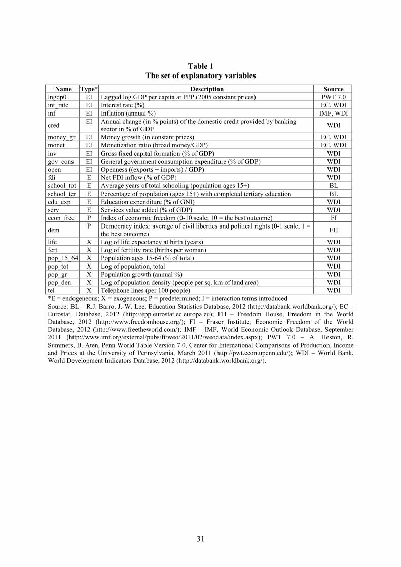
31

Table 1 The set of explanatory variables

Name Type* Description Source lngdp0 EI Lagged log GDP per capita at PPP (2005 constant prices) PWT 7.0 int_rate EI Interest rate (%) EC, WDI inf EI Inflation (annual %) IMF, WDI

cred EI Annual change (in % points) of the domestic credit provided by banking sector in % of GDP WDI

money_gr EI Money growth (in constant prices) EC, WDI monet EI Monetization ratio (broad money/GDP) EC, WDI inv EI Gross fixed capital formation (% of GDP) WDI gov_cons EI General government consumption expenditure (% of GDP) WDI open EI Openness ((exports + imports) / GDP) WDI fdi E Net FDI inflow (% of GDP) WDI school_tot E Average years of total schooling (population ages 15+) BL school_ter E Percentage of population (ages 15+) with completed tertiary education BL edu_exp E Education expenditure (% of GNI) WDI serv E Services value added (% of GDP) WDI econ_free P Index of economic freedom (0-10 scale; 10 = the best outcome) FI

dem P Democracy index: average of civil liberties and political rights (0-1 scale; 1 = the best outcome) FH

life X Log of life expectancy at birth (years) WDI fert X Log of fertility rate (births per woman) WDI pop_15_64 X Population ages 15-64 (% of total) WDI pop_tot X Log of population, total WDI pop_gr X Population growth (annual %) WDI pop_den X Log of population density (people per sq. km of land area) WDI tel X Telephone lines (per 100 people) WDI *E = endogeneous; X = exogeneous; P = predetermined; I = interaction terms introduced Source: BL – R.J. Barro, J.-W. Lee, Education Statistics Database, 2012 (http://databank.worldbank.org/); EC – Eurostat, Database, 2012 (http://epp.eurostat.ec.europa.eu); FH – Freedom House, Freedom in the World Database, 2012 (http://www.freedomhouse.org/); FI – Fraser Institute, Economic Freedom of the World Database, 2012 (http://www.freetheworld.com/); IMF – IMF, World Economic Outlook Database, September 2011 (http://www.imf.org/external/pubs/ft/weo/2011/02/weodata/index.aspx); PWT 7.0 – A. Heston, R. Summers, B. Aten, Penn World Table Version 7.0, Center for International Comparisons of Production, Income and Prices at the University of Pennsylvania, March 2011 (http://pwt.econ.upenn.edu/); WDI – World Bank, World Development Indicators Database, 2012 (http://databank.worldbank.org/).

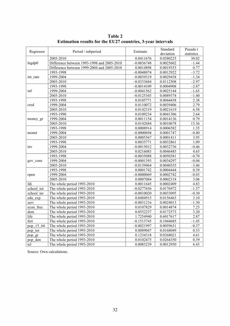
32

Table 2

Estimation results for the EU27 countries, 3-year intervals

Regressor Period / subperiod Estimate Standard deviation

Pseudo t statistics

2005-2010 0.8411676 0.0280225 30.02 Difference between 1993-1998 and 2005-2010 –0.0036748 0.0025602 –1.44 lngdp0 Difference between 1999-2004 and 2005-2010 0.0014898 0.0019353 0.77 1993-1998 –0.0048074 0.0012922 –3.72 1999-2004 –0.0039319 0.0029438 –1.34 int_rate 2005-2010 –0.0333684 0.0112508 –2.97 1993-1998 –0.0014109 0.0004908 –2.87 1999-2004 –0.0041562 0.0025144 –1.65 inf 2005-2010 –0.0125343 0.0089374 –1.40 1993-1998 0.0105771 0.0044438 2.38 1999-2004 0.0110072 0.0039406 2.79 cred 2005-2010 0.0142319 0.0021619 6.58 1993-1998 0.0109234 0.0041306 2.64 1999-2004 0.0011154 0.0014136 0.79 money_gr 2005-2010 0.0142684 0.0010678 13.36 1993-1998 0.0008914 0.0006582 1.35 1999-2004 –0.0000694 0.0001747 –0.40 monet 2005-2010 0.0005567 0.0001411 3.95 1993-1998 0.0035771 0.0032861 1.09 1999-2004 –0.0015012 0.0032736 –0.46 inv 2005-2010 0.0216083 0.0046485 4.65 1993-1998 –0.0035088 0.0050381 –0.70 1999-2004 –0.0001393 0.0034297 –0.04 gov_cons 2005-2010 –0.0139464 0.0040355 –3.46 1993-1998 0.0001742 0.0004444 0.39 1999-2004 –0.0000069 0.0002742 –0.03 open 2005-2010 0.0007084 0.0002318 3.06

fdi The whole period 1993-2010 0.0011645 0.0002409 4.83 school_tot The whole period 1993-2010 –0.0277656 0.0176972 –1.57 school_ter The whole period 1993-2010 –0.0010020 0.0033095 –0.30 edu_exp The whole period 1993-2010 0.0484915 0.0156463 3.10 serv The whole period 1993-2010 –0.0031216 0.0024013 –1.30 econ_free The whole period 1993-2010 0.0107829 0.0014874 7.25 dem The whole period 1993-2010 0.0552237 0.0172573 3.20 life The whole period 1993-2010 1.7254940 0.6017617 2.87 fert The whole period 1993-2010 –0.1513745 0.1044685 –1.45 pop_15_64 The whole period 1993-2010 –0.0021997 0.0059631 –0.37 pop_tot The whole period 1993-2010 0.0089047 0.0168049 0.53 pop_gr The whole period 1993-2010 0.1234318 0.0268021 4.61 pop_den The whole period 1993-2010 0.0102475 0.0264350 0.39 tel The whole period 1993-2010 0.0083239 0.0012950 6.43

Source: Own calculations.

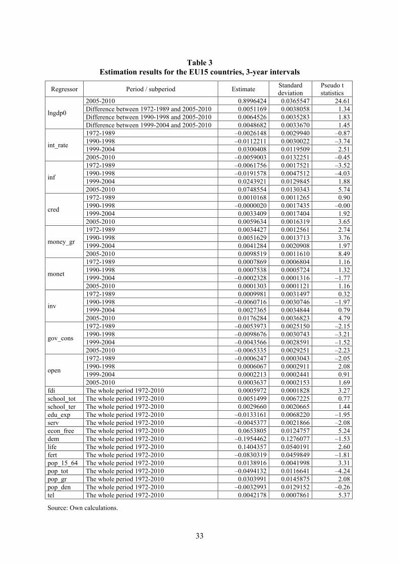
33

Table 3

Estimation results for the EU15 countries, 3-year intervals


Pseudo t statistics

2005-2010 0.8996424 0.0365547 24.61 Difference between 1972-1989 and 2005-2010 0.0051169 0.0038058 1.34 Difference between 1990-1998 and 2005-2010 0.0064526 0.0035283 1.83 lngdp0

Difference between 1999-2004 and 2005-2010 0.0048682 0.0033670 1.45 1972-1989 –0.0026148 0.0029940 –0.87 1990-1998 –0.0112211 0.0030022 –3.74 1999-2004 0.0300408 0.0119509 2.51 int_rate

2005-2010 –0.0059003 0.0132251 –0.45 1972-1989 –0.0061756 0.0017521 –3.52 1990-1998 –0.0191578 0.0047512 –4.03 1999-2004 0.0243921 0.0129845 1.88 inf

2005-2010 0.0748554 0.0130343 5.74 1972-1989 0.0010168 0.0011265 0.90 1990-1998 –0.0000020 0.0017435 –0.00 1999-2004 0.0033409 0.0017404 1.92 cred

2005-2010 0.0059634 0.0016319 3.65 1972-1989 0.0034427 0.0012561 2.74 1990-1998 0.0051629 0.0013713 3.76 1999-2004 0.0041284 0.0020908 1.97 money_gr

2005-2010 0.0098519 0.0011610 8.49 1972-1989 0.0007869 0.0006804 1.16 1990-1998 0.0007538 0.0005724 1.32 1999-2004 –0.0002328 0.0001316 –1.77 monet

2005-2010 0.0001303 0.0001121 1.16 1972-1989 0.0009981 0.0031497 0.32 1990-1998 –0.0060716 0.0030746 –1.97 1999-2004 0.0027365 0.0034844 0.79 inv

2005-2010 0.0176284 0.0036823 4.79 1972-1989 –0.0053973 0.0025150 –2.15 1990-1998 –0.0098676 0.0030743 –3.21 1999-2004 –0.0043566 0.0028591 –1.52 gov_cons

2005-2010 –0.0065335 0.0029251 –2.23 1972-1989 –0.0006247 0.0003043 –2.05 1990-1998 0.0006067 0.0002911 2.08 1999-2004 0.0002213 0.0002441 0.91 open

2005-2010 0.0003637 0.0002153 1.69 fdi The whole period 1972-2010 0.0005972 0.0001828 3.27 school_tot The whole period 1972-2010 0.0051499 0.0067225 0.77 school_ter The whole period 1972-2010 0.0029660 0.0020665 1.44 edu_exp The whole period 1972-2010 –0.0133161 0.0068220 –1.95 serv The whole period 1972-2010 –0.0045377 0.0021866 –2.08 econ_free The whole period 1972-2010 0.0653805 0.0124757 5.24 dem The whole period 1972-2010 –0.1954462 0.1276077 –1.53 life The whole period 1972-2010 0.1404357 0.0540191 2.60 fert The whole period 1972-2010 –0.0830319 0.0459849 –1.81 pop_15_64 The whole period 1972-2010 0.0138916 0.0041998 3.31 pop_tot The whole period 1972-2010 –0.0494132 0.0116641 –4.24 pop_gr The whole period 1972-2010 0.0303991 0.0145875 2.08 pop_den The whole period 1972-2010 –0.0032993 0.0129152 –0.26 tel The whole period 1972-2010 0.0042178 0.0007861 5.37


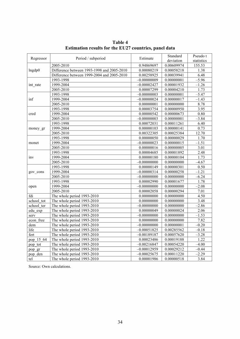
34

Table 4 Estimation results for the EU27 countries, panel data


Pseudo t statistics

2005-2010 0.94869697 0.00609974 155.53 Difference between 1993-1998 and 2005-2010 0.00080219 0.00058218 1.38 lngdp0 Difference between 1999-2004 and 2005-2010 0.00258925 0.00039941 6.48 1993-1998 –0.00000009 0.00000001 –5.96 1999-2004 –0.00002427 0.00001932 –1.26 int_rate 2005-2010 0.00007299 0.00004210 1.73 1993-1998 –0.00000003 0.00000001 –5.47 1999-2004 –0.00000024 0.00000017 –1.43 inf 2005-2010 0.00000001 0.00000000 8.78 1993-1998 0.00003754 0.00000950 3.95 1999-2004 0.00000542 0.00000673 0.80 cred 2005-2010 –0.00000003 0.00000001 –3.84 1993-1998 0.00072031 0.00011261 6.40 1999-2004 0.00000103 0.00000141 0.73 money_gr 2005-2010 0.00322305 0.00025384 12.70 1993-1998 0.00000050 0.00000029 1.70 1999-2004 –0.00000023 0.00000015 –1.51 monet 2005-2010 0.00000016 0.00000005 3.01 1993-1998 0.00004685 0.00001892 2.48 1999-2004 0.00000180 0.00000104 1.73 inv 2005-2010 –0.00000000 0.00000000 –4.67 1993-1998 0.00000149 0.00000301 0.50 1999-2004 –0.00000314 0.00000258 –1.21 gov_cons 2005-2010 –0.00000000 0.00000000 –6.24 1993-1998 0.00002990 0.00001677 1.78 1999-2004 –0.00000000 0.00000000 –2.08 open 2005-2010 0.00002058 0.00000294 7.01

fdi The whole period 1993-2010 0.00000000 0.00000000 4.50 school_tot The whole period 1993-2010 0.00000000 0.00000000 3.48 school_ter The whole period 1993-2010 –0.00000000 0.00000000 –2.86 edu_exp The whole period 1993-2010 0.00000049 0.00000024 2.06 serv The whole period 1993-2010 –0.00000000 0.00000000 –1.53 econ_free The whole period 1993-2010 0.00000000 0.00000000 7.82 dem The whole period 1993-2010 –0.00000000 0.00000001 –0.20 life The whole period 1993-2010 –0.00051825 0.00285562 –0.18 fert The whole period 1993-2010 –0.00189187 0.00057620 –3.28 pop_15_64 The whole period 1993-2010 0.00023486 0.00019188 1.22 pop_tot The whole period 1993-2010 –0.00216847 0.00054220 –4.00 pop_gr The whole period 1993-2010 –0.00012959 0.00029212 –0.44 pop_den The whole period 1993-2010 –0.00025675 0.00011220 –2.29 tel The whole period 1993-2010 0.00001986 0.00000518 3.84


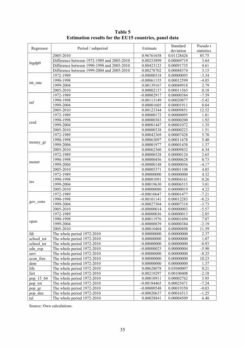
35

Table 5 Estimation results for the EU15 countries, panel data


Pseudo t statistics

2005-2010 0.96761658 0.01128426 85.75 Difference between 1972-1989 and 2005-2010 0.00253899 0.00069719 3.64 Difference between 1990-1998 and 2005-2010 0.00423123 0.00091735 4.61 lngdp0

Difference between 1999-2004 and 2005-2010 0.00278702 0.00088374 3.15 1972-1989 –0.00000318 0.00000095 –3.34 1990-1998 –0.00061155 0.00012599 –4.85 1999-2004 0.00139167 0.00049918 2.79 int_rate

2005-2010 0.00002137 0.00011565 0.18 1972-1989 –0.00002917 0.00000384 –7.59 1990-1998 –0.00113149 0.00020877 –5.42 1999-2004 0.00001605 0.00001911 0.84 inf

2005-2010 0.00123344 0.00009851 12.52 1972-1989 0.00000172 0.00000095 1.81 1990-1998 0.00000383 0.00000200 1.92 1999-2004 0.00001447 0.00001072 1.35 cred

2005-2010 0.00000338 0.00000223 1.51 1972-1989 0.00042369 0.00007428 5.70 1990-1998 0.00063097 0.00011678 5.40 1999-2004 0.00001977 0.00001438 1.37 money_gr

2005-2010 0.00062360 0.00009832 6.34 1972-1989 0.00000328 0.00000124 2.65 1990-1998 0.00000456 0.00000628 0.73 1999-2004 –0.00000148 0.00000036 –4.17 monet

2005-2010 0.00005371 0.00001108 4.85 1972-1989 0.00000000 0.00000000 4.32 1990-1998 0.00001091 0.00004161 0.26 1999-2004 0.00019630 0.00006515 3.01 inv

2005-2010 0.00000080 0.00000019 4.22 1972-1989 –0.00010647 0.00001477 –7.21 1990-1998 –0.00101141 0.00012283 –8.23 1999-2004 –0.00027304 0.00007318 –3.73 gov_cons

2005-2010 –0.00000014 0.00000003 –5.57 1972-1989 –0.00000036 0.00000013 –2.85 1990-1998 0.00011976 0.00001694 7.07 1999-2004 –0.00000839 0.00000384 –2.19 open

2005-2010 0.00010404 0.00000898 11.59 fdi The whole period 1972-2010 0.00000000 0.00000000 2.37 school_tot The whole period 1972-2010 0.00000000 0.00000000 1.07 school_ter The whole period 1972-2010 –0.00000000 0.00000000 –0.93 edu_exp The whole period 1972-2010 –0.00000023 0.00000004 –5.90 serv The whole period 1972-2010 –0.00000000 0.00000000 –8.25 econ_free The whole period 1972-2010 0.00000000 0.00000000 10.23 dem The whole period 1972-2010 0.00000000 0.00000000 1.37 life The whole period 1972-2010 0.00628078 0.03040007 0.21 fert The whole period 1972-2010 –0.00219297 0.00100408 –2.18 pop_15_64 The whole period 1972-2010 0.00010911 0.00002762 3.95 pop_tot The whole period 1972-2010 –0.00184465 0.00025471 –7.24 pop_gr The whole period 1972-2010 –0.00000548 0.00019350 –0.03 pop_den The whole period 1972-2010 –0.00020637 0.00016513 –1.25 tel The whole period 1972-2010 0.00028841 0.00004509 6.40


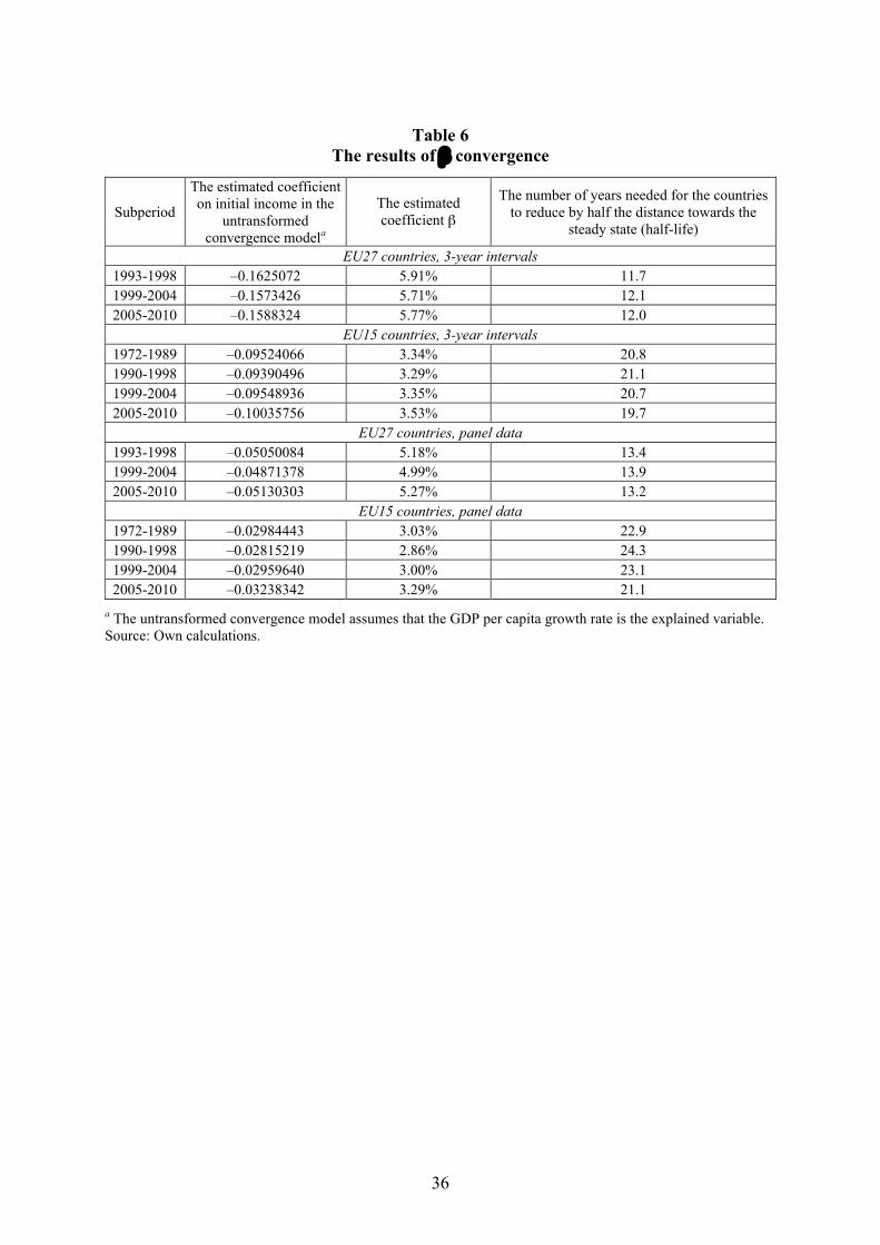
36

Table 6

The results of β convergence

Subperiod

The estimated coefficient on initial income in the

untransformed convergence modela

The estimated coefficient β

The number of years needed for the countries to reduce by half the distance towards the

steady state (half-life)

EU27 countries, 3-year intervals 1993-1998 –0.1625072 5.91% 11.7 1999-2004 –0.1573426 5.71% 12.1 2005-2010 –0.1588324 5.77% 12.0

EU15 countries, 3-year intervals 1972-1989 –0.09524066 3.34% 20.8 1990-1998 –0.09390496 3.29% 21.1 1999-2004 –0.09548936 3.35% 20.7 2005-2010 –0.10035756 3.53% 19.7

EU27 countries, panel data 1993-1998 –0.05050084 5.18% 13.4 1999-2004 –0.04871378 4.99% 13.9 2005-2010 –0.05130303 5.27% 13.2

EU15 countries, panel data 1972-1989 –0.02984443 3.03% 22.9 1990-1998 –0.02815219 2.86% 24.3 1999-2004 –0.02959640 3.00% 23.1 2005-2010 –0.03238342 3.29% 21.1

a The untransformed convergence model assumes that the GDP per capita growth rate is the explained variable. Source: Own calculations.

β-convergence stability among “old” and “new” eu countries

Documents