1378100

MULT I I>HASE NUMERICAL MODELLING

OF1 THICKENING AND SEDIMENTATION

BY

CHRISTOPHER JOHN|j3AI LEYBSc (Honours)

Thesis submitted to the Council for National Academic Awards in partial fulfilment of the requirements for the Degree of Doctor of Philosophy.

Centre for Numerical Modelling and Process Analysis School of Mathematics, Statistics and Computing

Thames Polytechnic London.

In collaboration with Department of Trade and Industry, Warren Springs Laboratories

of

JULY 1988

CONTENTS

ABSTRACT

ACKNOWLEDGEMENTS VI

CHAPTER 1 : INTRODUCTION

1.1 Sedimentation and Thickening

1.2 Literature Review

1.3 Aims of Research

1

2

3

11

CHAPTER 2 : EXPERIMENTAL METHOD FOR NONFLOCCULATED BATCH SEDIMENTATION

2.1

2.3

Introduction

2.2 Apparatus used

Materials used

2.4 Experimental procedure

2.4.1 Calibrations

2.4.2 Experimental runs

14

15

16

16

21

23

25

CHAPTER 3 : OBTAINING CONTINUOUS GRAVITY THICKENER DATA

3.1

3.4

Introduction

3.2 Apparatus used

3.3 Experimental procedure

Results

31

32

34

35

38

ii

CHAPTER 4 : A NUMERICAL MODEL FOR NON-FLOCCULATEDBATCH SEDIMENTATION 55

4.1 Introduction 56

4.2 Governing Equations 58

4.2.1 Solid phase continuity 59

4.2.2 Solid phase momentum 59

4.2.3 Concentration balance 60

4.2.4 Total volumetric balance 61

4.2.5 Boundary conditions 61

4.3 Discretised equations 61

4.3.1 Solid phase continuity 63

4.3.2 Solid phase momentum 65

4.3.3 Concentration balance 66

4.3.4 Total volumetric balance 67

4.4 Incorporating packing theory 67

4.4.1 Packing Model 68

4.4.2 Further densification of sediment 72

4.5 Solution procedure 73

4.6 Comparisons with Holdich data 80

4.7 Comparisons with Experimental data 90

4.7.1 One phase comparisons 91

4.7.2 Two phase comparisons 103

4.7.3 Three phase comparisons 113

iii

CHAPTER 5 : MODELLING A CONTINUOUS GRAVITY THICKENER

5.1 Introduction

5.2 Governing Equations

5.2.1 Solid phase equations

5.2.2 Fluid phase equations

5.2.3 Boundary conditions

5.3 Control volume representation

5.4 Discretised equations

5.4.1 Solid phase continuity

5.4.2 Solid phase momentum

5.4.3 Total volumetric balance

5.5 Solution procedure

5.6 Comparisons with experimental data

5.6.1 Galena thickener

5.6.2 Fluorite thickener

5.6.3 Barytes thickener

122

123

124

124

125

126

126

130

132

133

133

134

137

138

144

148

CHAPTER 6

6.1

6.2

A NUMERICAL MODEL FOR FLOCCULATED BATCH SEDIMENTATION

Introduction

Floe build up in free settling region

6.2.1 Smoluchowski population balances

6.2.2 Incorporating floe build up viacontinuity and momentum equations

6.3 Compression in the sediment zone

6.3.1 Incorporating compression via the momentum equations

6.3.2 Incorporating packing theory

6.4 Solution procedure

6.5 Comparisons with Holdich data

153

154

156

157

160

163

164

165

165

167

IV

CHAPTER 7 : CONCLUSIONS 175

7.1 Experimentation I?6

7.2 Mathematical Modelling 177

APPENDIX 180

NOMENCLATURE 181

REFERENCES 184

ABSTRACT

Phenomena that involve the settling of participates in a host fluid are

encountered in many practical systems which find applications in many

areas of industry. A numerical model has been developed to simulate the

settlement of non-flocculated and flocculated particulate suspensions in

batch sedimentation. The non flocculated mode of the model is extended

to predict the performance of a continuous gravity thickener.

The various particle species within the particulate suspension are

represented as separate phases with distinct concentrations and

velocities. A multiphase representation of the settling process gives

greater detail of the interactions present between the particulates.

The build up of the sediment as well as a prediction of the compression

point, for flocculated suspensions, is modelled using a revised version

of packing theory. The build up of floes in the free settling region is

incorporated via population balances.

Also, as well as the above theoretical work, experimentwal work has been

undertaken to obtain data for non-flocculated suspensions. For batch

sedimentation this data is in the form of density profiles and for the

continuous thickener it is in the form of concentration profiles. The

proposed model compares favourably with this experimental data and gives

closer predictions than does a model representing the state of the art,

at this point in time, for non-flocculated batch sedimentation.

VI

ACKNOWLEDGEMENTS

I would like to express my gratitude to Professor Mark Cross and Dr

Dilwyn Edwards for their help and guidance throughout this project.

I also wish to thank Dr Peter Tucker and Phil Parsonage who helped me

with the experimental work. I would also like to acknowledge the

financial and experimental support of Warren Spring Laboratory through a

SERC-CASE studentship.

My sincerest thanks go to my family and friends for all their help and

encouragement.

Finally, many thanks to Edie McFall for the typing of this thesis.

NIO

- I -

- 2 -

1.1 Sedimentation and Thickening

Solid-liquid separation has ^widespread applications in the industrial

world. Examples of some processes which involve solid-liquid separation

are: -

1) Sedimentation and thickening.

2) Centrifugation.

3) Hydrocyclones.

4) Flotation.

All the above processes involve the movement of solids and liquid due to

an applied force acting on these phases. The process of importance with

regards to this thesis is "Sedimentation and Thickening". Sedimentation

involves the movement of particulates in a host fluid due to the action

of gravity. Thickening involves sedimentation and compaction taking

place in a large circular tank containing a particulate slurry. The

compaction occurs in the sediment region, at the base of the tank, which

may be compressible or incompressible depending on the nature of the

particulate slurry. To increase the rate of thickening and to enable

very fine particulates to settle, flocculants are used. Flocculants are

chemicals which break down the repulsive forces between particles and

build bridges linking the particles. This enables particles to

agglomerate and settle as larger masses known as floes. Thickening is a

favoured method of large scale dewatering because of its cost and

simplicity. The main design requirement of a thickener is its surface

area, this must be large enough to enable solids throughput so that

solids do not build up in the thickener and, hence, appear in the

overflow. To enable greater compaction of the sediment, depth is also

said to be important. Over the last ten years major advances have taken

place in this field which include; improvements in synthetic

- 3 -

flocculants, better thickener designs and a greater understanding of the

principles involved.

1.2 Literature Review

There have been numerous experimental and theoretical investigations

into the sedimentation of particles in a fluid. The first analysis was

by Stokes (1851) who observed the rate of fall of a single spherical

particle in a quiescent Newtonian fluid at low Reynolds number which led

to his well-known law:

where Ut is the terminal velocity of a sphere, d its diameter, ps

its density, pf the fluid density, Mf the fluid viscosity and g

the gravitational constant. For solid concentrations, by volume, above

1* the average settling velocity of the monodispersed suspension will be

noticeably lower than that predicted by equation (1.1). This is due to

a phenomena known as hindered settling. This effect is incorporated by

multiplying equation (1.1) by a hindered settling function to give the

solids velocity. Two of the most widely used empirical functions are

those by Richardson and Zaki (1954) and Barnea (1973). Richardson and

Zaki proposed the following correlation between ju-j. and solids

velocity, Us ;

* = (l-S) n (1.2)

where S is solids concentration and n is a value dependent on

Reynolds number. Barnea (1973) gave the following explanation for

hindrance:

- 4 -

1) HYDROSTATIC EFFECT: The suspension density is greater than that of

the fluid alone and consequently the buoyancy force is greater.

Therefore the suspension density should be used in equation (1.1.)

instead of the fluid density.

2) MOMENTUM TRANSFER EFFECT: The presence of other particles effects

the transfer of momentum between each particle and the fluid. This

effect is related to the "apparent" bulk viscosity of the suspension.

Barnea (1973) related solids velocity and terminal velocity using the

above effects. The momentum transfer effect is incorporated by using a

relationship between suspension and fluid viscosities.

The majority of particulate mixtures are not monodispersed as they

contain particles of different sizes, density and shape. These

polydispersed mixtures have been modelled by Lockett and Al-Habbooby

(1973, 1974) who carried out experiments on binary particulate mixtures.

They used the monodispersed Richardson and Zaki (1954) correlation to

predict the solids velocity of each phase where the total particle

concentration is used to correct the terminal velocity of each phase as

predicted by equation (1.1). Mirza and Richardson (1979) extended the

Lockett and Al-Habbooby model to predict the sedimentation of multisized

particle systems. They compared their model predictions with

experimental results in the form of velocity against voidage plots. As

with the Lockett and Al-Habbooby comparisons they found that the model

overpredicted sedimentation velocities. To remedy this effect they

applied a correction factor of (voidage) 0 ' 4 to the velocities, this gave

satisfactory comparisons with their experimental results. In a similar

study Selira et al (1983) proposed that the Stokes velocity of phase i,

say, should be modified by replacing the fluid density in equation (1.1)

- 5 -

by the average density of a suspension consisting of fluid and particles

of size smaller than i. Obviously this is only valid for multisized

systems but Selim obtained good comparisons between his experimental

results and model predictions. For a polydisperse system the settling

of the suspension will result in the formation of distinct zones. The

lowest zone just above the sediment containing all particulate phases at

their initial concentrations, with each successive region above

containing one fewer phase than the zone below (i.e. fastest settling

phase. The above models use the Richardson and Zaki empirical

correlation and mass balances to calculate, iteratively, the velocity

and solids concentrations of each phase in each zone. In these models

no account is taken of the sediment build up at the base. In a short

communication Masliyah (1979) extended the governing equation for

hindered settling to incorporate different densities as well as sizes.

He proposed the use of the total suspension density instead of the fluid

density in the buoyancy term and suggested the use of the Richardson and

Zaki (1954) or the Barnea (1973) correlations for the momentum transfer

effects. Unfortunately no detailed comparisons with experimental data

was made but the use of the suspension density instead of the fluid

density is obviously a correct assumption. This has been a debating

point in the literature for many years but its obvious that the buoyancy

is not caused by the density difference between the suspended particles

and surrounding fluid, but is the result of the imbalance between the

pressures exerted on each of the settling units by the fluid, which is a

verticle hydraulic pressure gradient. In a suspension this gradient is

determined by the suspension density and not by the fluid density. The

effect of buoyancy is less than that of structure which is determined

essentially by the suspension viscosity. Barnea (1973) gave a detailed

review of suspension viscosity models and also proposed his own which is

used in this thesis.

- 6 -

The design of thickeners is based on calculating the unit area. This is

the surface area of a thickener required to handle unit weight of solids

in unit time, or simply the area per unit throughout required to give a

specified dewatering. The principle investigators into thickener design

were Coe and Clevenger (1916). The objective of their work was to

present a method to calculate the area of a thickener from batch

sedimentation tests. This test consists of filling a glass tube with

slurry at known concentration and letting the solids settle. For steady

state continuous thickening Coe and Clevenger derived the following

formula:

G = l l (1.3)

S " Su

where G is the solids handling capacity or the flux of solids moving

towards the underflow, S is the solids concentration of a batch test,

U its settling velocity and Su is the solids concentration at the

thickener underflow. The method requires that pulps of various

concentrations between the thickener feed and underflow be prepared as

batch tests in sedimenting columns. These suspensions are allowed to

settle and the rate of fall of the supernatant/pulp interface is noted.

Using equation (1.3) a flux against concentration plot can be

constructed. The minimum value of flux is taken as the solids handling

capacity of the thickener and used in the design. The thickener area

can be calculated from this flux value, where flux is defined as

thickener feed rate divided by surface area. This approach makes the

following assumptions:

1) No segregation occurs.

2) Most flux limiting concentration lies in the free settling

zone.

- 7 -

3) Solids velocity is independent of concentration.

The Coe and Clevenger (1916) method held favour for nearly forty years

until Kynch (1952) produced his mathematical analysis of the batch

settling curve. Kynch based his analysis on the same assumptions as

above and concluded that concentrations would propogate upwards from the

bottom of a suspension, each at it own constant velocity equal to the

tangent of the batch-flux curve at that concentration. He further

showed that the settling velocities of higher concentrations could be

obtained from the batch settling curve of a suspension initially at a

uniform lower concentration. The batch settling curve being a plot of

supernatant/pulp interfce height against time. Talmage and Fitch (1955)

used Kynch's mathematics to estimate thickener area from a batch

settling curve. The curve is obtained from a batch test whose initial

slurry concentration is equal to that of the thickener feed. This is a

graphical technique which requires locating the compression point on the

batch settling curve and drawing a tangent to it. From this both the

limiting concentration and its settling velocity can be calculated.

Using equation (1.3) the corresponding solids handling capacity is

calculated from which the thickener area is estimated. The Talmage and

Fitch model shows a definite improvement over Coe and Clevenger in that

it is experimentally simpler with all data being obtained from one

batch settling curve. The concensus of opinion, Pearce (1977), is that

the Talmage and Fitch procedure overpredicts thickener area while the

Coe and Clevenger method underpredicts thickener area. Therefore it is

safer to use Talmage and Fitch's methods as this ensures throughput and

no presence of solids in the overflow of the thickener.

Kynch's (1952) analysis has become the basis of the solids flux theory

of which graphical techniques based on the batch settling curve (Talmage

- 8 -

and Fitch (1955)), and the batch flux curve, (Yoshioka (1957) and

Hassett (1965)), have been proposed. The major drawback with these

techniques is that they rely on the assumptions that solids velocity is

a unique function of solids concentration. This certainly is not the

case with flocculated pulps although it may be true for some

metallurgical suspensions, Holdich (1983).

For flocculated suspensions particles collide and some agglomeration may

occur causing floes to form. Michaels and Bolger (1962) correlated

experimental data by means of a modified form of the Richardson and Zaki

(1954) equation. They assumed that each floe was spherical in shape and

that water within the floe moved with it. Based on these assumptions

the movement of floes in the free settling region are expected to follow

equation (1.2); but with solids concentration replaced by floe

concentration and solids density replaced by floe density. This

equation is valid in the free settling region but does not take into

account floe formation and is invalid in the compression zone where

floes lose their individual identity and become part of a compressible

structure. In the compression region Michaels and Bolger (1962) used a

concept similar to the Terzargi soil consolidation model to develop a

model predicting the subsidence rate in the compression zone. They

assume that the compressing pulp will have a resistivity and compressive

yield which are both dependent on solids concentration.

Shirato et al (1970) confirmed experimentally the assumption that solids

pressure is dependent on solids concentration only. For permeability he

assumed the Kozeny relationship and obtained good comparisons between

predicted and measured concentration profiles for ferric oxide and zinc

oxide suspensions. Kos (1974) reflected the assumption that

permeability was a function of concentration and dynamic pressure. He

- 9 -

also found that solids pressure is approximately proportional to solids

concentration.

Gaudin and Fuerstenau (1962) carried out experiments on flocculated

Kaolin suspension; for the compression regime they applied Poiseuilles

law to the flow of liquid through pores in the pulp. The pores were

considered to have a size distribution given by a Schuhmann (1940)

distribution. This model requires knowledge of the number and sizes of

the pores present in a pulp and is therefore difficult to apply.

Coe and Clevenger (1916) observed the subsidence rate for pulps having

concentrations in the compression regime. They deduced that compaction

was a function of time; a conclusion which is now known to be invalid,

Fitch (1975). Dell and Keleghan (1973) used a cleverly designed

pressure measuring method to show that solids velocity was not dependent

on solids concentration for flocculated material. They found that the

mass of material above a fixed height did not fall off linearly as

predicted by Coe and Clevenge (1916) and Kynch (1952), but

exponentially. Dick (1967) suggested a deviation factor from ideality,

the retardation factor, which varies exponentially with solids

concentration. Dick (1972) also emphasised the point that for

compressible pulps the effects of sedimentation and compaction must be

combined in order to understand performance.

Adorjan (1975) also assumed solids pressure and permeability to be

dependent on solids concentration. With the assumption that no

segregation is present and that permeability is obtained from

compression permeability cell tests, Adorjan used his theory to predict

thickener unit areas via numerical integration to obtain height

concentration profiles.

- 10 -

Dixon (1977, 1978) proposed the use of a force balance approach as well

as »ass balances for the fluid and particulate phases present in

non-flocculated and flocculated systems. He assumed the presence of

only one solid phase and discussed the forces present in the system. He

concluded that: "There is no solids flux limitation associated with the

free settling zone in a continuous gravity thickener". Holdich (1983)

carried out experiments to obtain concentration profiles for the

settlement of both flocculated and non-flocculated suspensions. He used

the force balance approach proposed by Dixon to assess the relevance and

completeness of the constituent terms. He assumed no segregation to

take place and proposed an extra term known as transient solids pressure

to be present throughout the suspension. This term is introduced to

explain why concentration gradients are present in the free settling

region. Via his experimental results he concludes that the commonly

made assumption of solids pressure being dependent on solids

concentration is too simplistic.

Pitch (1983), Tiller (1981) and Concha (1987) revised the classical

Kynch theory to be valid for compressible suspensions. Fitch and Tiller

both propose alternative graphical procedures to obtain suspension

concentrations and their corresponding settling velocities. Concha

reports that both the Fitch and Tiller revisions violate the

fundamentals of the Kynch theory. Concha used a numerical procedure

incorporating a solids pressure term, dependent on solids concentration,

beyond the compression regime. Using this procedure he obtains solids

concentrations over time throughout a batch vessel. As with all other

authors he assumes that no segregation occurs in the free settling

region.

- 11 -

Although thickener throughput is controlled by area it is believed that

underflow concentration is determined by thickener depth. Talmage and

Fitch (1955) extended their graphical procedure to predict thickener

depth needed to give a desired underflow. Pearce (1977) reports that

this method may give unrealistic results and states the "three foot

rule", which states that if the predicted depth is over 3ft then the

area is increased so that the depth is equal to 3ft. This gives

underflow concentrations closer to those predicted by the Talmage and

Fitch (1955) compression test. This is adequate for most metallurgical

operations but fails for flocculated suspensions and at this point in

time no sound theory for the effects of depth has been developed, Pearce

(1977).

As can be deduced from the above review a lot of controversy still

exists as to the principles governing sedimentation and thickening,

especially for compressible suspensions. Although much research has

been undertaken the operation of a thickener remains more of an art than

a science and there is still a need for models and techniques which can

be used to predict thickener performance.

1.3 Aims of Research

The thickening of a particulate slurry is essentially a multiphased

phenomena. Particles of different sizes, shapes and densities may be

present and their rate of settlement and compaction characteristics will

be dependent on these values. Further, the effect of flocculation will

give rise to the formation of floes which will have distinct sizes,

shapes and densities. The work of thickening and sedimentation, to

date, has mostly been undertaken to investigate either the free settling

region or the sediment region. For batch sedimentation the vast

majority of work is based on the empirical correlations between solids

- 12 -

settling velocity and solids terminal velocity. No account in these

models is made of where the sediment interface is (i.e. the compression

point). Also the internal structure of the sediment and the changes in

it during sediment build up are ignored. For flocculated slurries no

model exists which predicts floe build up in the free settling zone, it

is always assumed that floes exist of unique size, shape and density,

in the case of thickener design the majority of methods are graphical in

nature and are based on the batch settling curve. Once again these

methods do not predict sediment characteristics and are obviously

limited in their use.

The main aim of this research is to develop a numerical model that will

represent thickening and sedimentation in much greater detail than

models presently used. This is achieved by breaking down the solids

distribution in the slurry into a number of distinct phases and also

predicting sediment build up using a revised version of packing theory.

This model will have three modes of operation:

1) Non Flocculated Batch Sedimentation.

2) Non Flocculated Continuous Gravity Thickening.

3) Flocculated Batch Sedimentation.

The simplest type of model is for mode (1), above, where the other two

modes are simply extensions of this model. Using the force balance

approach where each solid phase has associated with it equations of mass

and momentum, these extensions involve changing and adding terms to the

basic transport equations representing each phase present in the system.

In addition to the theoretical work, another aim of this research is to

obtain good quality experimental data. This will enable verification of

the proposed models. Also compared with some of the experimental data

- 13 -

are predictions by the Selira (1983) model which represents one of the

better models for batch sedimentation. This model has been extended to

cope with multidensity as well as multisized suspensions.

- 14 -

CHAPTER TWO

EXPERIMENTAL METHOD FOR NON

FLOCCULATED BATCH SEDIMENTATION

- 15 -

2.1 Introduction

Experimental work into the sedimentation of non-flocculated slurry's has

been undertaken by a number of authors, although the amount of useful

data especially for this study is limited. Two types of experimental

technique can be employed:

1) Direct measurements; where the slurry has to be disturbed.

2) Indirect measurements; where data is recorded without disturbing the

slurry.

Direct measurements involve obtaining samples throughout the vessel.

This will enable concentrations to be calculated at different locations

in the vessel. To understand the full settling behaviour of the slurry

undergoing batch sedimentation the experiment must be repeated several

times, under identical conditions, so that samples can be obtained at

different points in time. This procedure is prone to large errors.

Indirect measurements obtain data (i.e. concentrations, velocities,

density changes, etc) predicting the settling behaviour using devices

that do not disturb the settling process. A major amount of the

experimental work into sedimentation of non-flocculated slurry's has

been to obtain the velocities at which each zone in the free settling

region descends, see Davies (1968), Mirza (1978) and Selim (1983). This

involves colouring each size fraction and recording the rate of fall of

each zone (i.e. the velocity of the fastest phase present in each zone)

throughout the experiment. Concentration profiles have also been

obtained using electrical conductivity, see Holdich (1983). The aim of

the following study is to use pressure transducers to obtain density

changes during the sedimentation of a multiphase particulate mixture.

- 16 -

2.2 Apparatus used

The experimental setup, see figure 2.1, consists of a perspex tube,

eight pressure transducers, a voltmeter, a junction box and a two pen

plotter. The perspex tube, see figure 2.2, is of height 60cm and

internal diameter 5.2cm. Measuring tape is fixed to the outside of the

tube. Before the transducers could be used each was subjected to a

vacuum and soaked overnight in water. This eliminates any trapped air,

which due to its compressibility would enable the transducer to give

erroneous results. The transducers are inserted, using silicon rubber,

into holes situated at 5cm intervals from the base of the tube upwards.

The front section of each transducer just protruding into the internal

part of the tube. A voltage is applied to the circuit via a voltmeter.

The juction box acts as a connection between the voltage input,

transducers and plotter. The connections inside the junction box were

cleaned and re-soldered before being used. The plotter is able to

monitor two transducers at a time and is sensitive down to O.OOSmV with

O.SmV F.S.D. (full scale deflection).

2.3 Materials used

Four different solids and three different liquids, see table 2.2 are

used. The overall size range of each material used is:

Material Size range (a)

Glass (soda) Ballontini 20 - 100/u

Glass (lead) Ballontini 30 - 500n

Copper 30 - 70u

Quartz 150 - 250w.

Table 2.1 Size range of solids.

- 17 -

SETTLING

COLUMN

MAINS

PRESSURE

TRANSDUCERS

VOLTMETER

JUNCTION

BOX

PLOTTER

Figure 2.1 Diagram of experimental setup

- 18 -

va^:-^'v^»t'l^t ••>:';$**&>%$:•'.

Figure 2.2 Perspex tube with transducers

- 19 -

The shape factor used in this analysis is given by

De5 DAV (2.1)

where « is the "effective volumetric" shape factor, DAV is the

average diameter of the particles and De is the diameter of a sphere

with volume equal to a particle of diameter DAV . Ballontini and copper

are spherical, see figure 2.3, therefore the shape factor is 1*0.

Quartz is an angular material and a shape factor commonly used is 0-86,

see Cross (1985). The densities for each solid material is calculated

using a pycnometer. This device estimates the volume of solid material

of known mass in a cup. The density is calculated via

P-* (2.2)

where p is the density, M the mass and V the calculated volume.

The densities calculated using the above method were very close to the

makers quoted values and these are the values used.

The glucose solution is made up in the laboratory by adding 389.8

grammes of sugar and 756.6 grammes of water for every litre of solution

required. The densities of each liquid is calculated using a 50cc

weighing bottle. The mass of liquid that fully occupies the bottle is

calculated by:

Mass of empty bottle = M l

Mass of full bottle = M2

Mass of liquid of volume 50cc = M 2 - Mj.

- 20 -

fi^^ifiSy

a) Ballontini b) Copper

c) Quartz

Figure 2.3 Photomicrographs of solids used for batch sedimentation

- 21 -

The densities are then calculated using equation 2.2. The viscosities

are the makers quoted values. All viscosity and density values are at

roon temperature (i.e. 20*C)

2.4 Experimental procedure

The following procedure will calculate the density changes in the

perspex tube due to the movement of the particulates in the fluid

particle mixture. For each transducer a linear relationship between

pressure and voltage will exist:

P = KV + C (2.3)

where P is the pressure acting on the transducer, V is the voltage

corresponding to this pressure and K,C are constants. The pressure

can also be calculated using the effective hydrostatic pressure

equation:

P = hpBg (2.4)

where h is the height of mixture above the transducer, PB the bulk

average mixture density and g the gravity constant.

Therefore, given a suspension of uniform concentration (volume

fractions) and density throughout, the above relationships, equations

(2.3) and (2.4), can be used to find the mixture density above a

transducer at different points in time during the settlement of the particulates. The initial mixture density is calculated via:

NSOL

S i p i (2-5)

- 22 -

Solid material

Glass (soda) Ballontini

Glass (lead) Ballontini

Copper

Quartz

Density(Kg/M 3 )

2480

2950

8930

2600

Shape factor

1

1

1

86

Liquid

Water (distilled)

Diethylene Glycol

Glucose Solution

Density(Kg/M 3 )

1000

1115

1149

Viscosity(Kg/MS)

0.001

0.014

0.004

Table 2.2 Material Properties.

- 23 -

where pf is the fluid density and PJ is the solid phase density for

phase i. F and S^ are the volume fractions for the fluid and solid

phases respectively. If the mass of each solid phase in the mixture is

MJ and the volume of the fluid, calculated using a SOOcc measuring

cylinder, is VF then the total volume of the mixture in the perspex

tube is:

NSOL

P~ (2 ' 6)

The solid and fluid volume fractions are calculated via

Mi i=l... ,NSOL (2.7)PivM

F = rr (2.8)VM

Using equations (2.5), (2.6), (2.7) and (2.8) the initial density of the

mixture is calculated. The pressure and voltage corresponding to the

initial density are calculated using equations (2.3) and (2.4). During

the settling process the plotter monitors the decrease in the voltage

output from the transducer over time. Using this graphical output and

equations (2.3) and (2.4) the decrease in the density of the mixture

above the transducer can be calculated.

2.4.1. Calibrations

A 5v voltage is applied to the circuit via the voltmeter for the

following calibrations as well as all experimental runs. Each pressure

transducer is calibrated to obtain a pressure-voltage relationship.

- 24 -

This involves adding distilled water to the tube and recording the

height of water above the transducer as well as the voltage deflection

on the plotter. The pressure after each addition of water is calculated

using equation (2.4) where pB is the density of water. Applying

regression analysis to the pressure, voltage data a linear relationship

is obtained, see equation (2.3).

At this point in the analysis it was noticed that only transducers one

and four could be measured down to an accuracy of O.OOSmv. All other

transducers had a measured accuracy down to 0.02mv or higher. This is

due to the voltage output being higher for all transducers except one

and four. Therefore, to obtain a good degree of accuracy, in interpret­

ing the graphical output, only transducers one and four could be used.

For the experimental runs transducer one was exchanged with transducers

two and three and recalibrated at these new positions. The pressure-

voltage relationships are:

Transducer one:

P = 1831V - 11 (2.9)

Transducer one (at second transducer location):

P = 1831V - 11 (2.10)

Transducer one (at third transducer location):

P = 1781V (2.11)

- 25 -

Transducer four:

P = 1818V. (2.12)

2.4.2 Experimental runs

Experimental data has been obtained for a number of one, two and three

phase experiments, see tables 2.4, 2.5 and 2.6. Each solid phase is

obtained by sieving the solid material. The particle size representing

each phase is taken as the mean aperture size of the two sieves used,

see table 2.3.

Sieve sizes (M) Particle size (n) Sieves used

38 41-5 38-45

45 56-5 38-75

63 60 45-75

75 69 63-75

90 76-5 63-90

150 120 90-150

180 200 150-250

250 220 180-250

300 275 250-300

355 302-5 250-355

425 327-5 300-355

500 362-5 300-425

462-5 425-500.

Table 2.3 Sieve and phase sizes.

ONE PHASE EXPERIMENTS

SOLID

Exp

one

Glas

s (lead)

Exp

two

Glas

s (lead)

Exp

three

Copp

er

Exp

four

Glass

(lea

d)

Exp

five

Glass

(lea

d)

Exp

six

Glass

(lead)

Exp

seven

Glas

s (l

ead)

Exp

eight

Glass

(lea

d)

Exp

nine

Glass

(lead)

Exp te

n Glass (l

ead)

Exp

eleven Gl

ass

(lead)

DIAM(n)

120

275

56-5

275

275

275

275

76-5

76-5

76-5

220

CONC

0-078

0-078

0-0138

0-078

0-1128

0-25

0-35

0-078

0-1128

0-25

0-1

LIQUID

Glycol

Glycol

Glycol

Glycol

Glycol

Glycol

Glycol

Glycol

Glycol

Glycol

Glycol

TRANSDUCER

one

one

two

thre

e

thre

e

thre

e

thre

e

thre

e

thre

e

thre

e

thre

e

to OJ

Table

2.4

Details for

one

phase

experiments

TWO-PHASE EXPERIMENTS

Exp

one

Exp

two

Exp

three

Exp

four

Exp

five

Exp

six

Exp

seven

Exp

eight

Exp

nine

SOLID

Copper

Copper

DIAM(n)

56-5

56-5

Glass

(lead)

327-5

Glass

(soda)

69

Quartz

Copper

200

Glass

(lead)

275

56-5

Glass

(lead)

302.5

Glass

(lead)

220

CONC

0- 0- 0- 0- 0- 0- 0- 0- 0-

026

0127

0725

1314

0771

039

034

039

09093

SOLID

Glass

Glass

Glass

Glass

Glass

Glass

Glass

Glass

Glass

(lead)

(lead)

(lead)

(soda)

(soda)

(lead)

(lead)

(lead)

(lead)

DIAM(M)

76-5

302.5

120

41-5

60 120

76-5

41-5

76-5

CONC

0 0 0 0 0 0 0 0 0

•076

•077

•0725

•049

7

•1212

•039

•098

•039

•09093

LIQUID

Glycol

Glycol

Glycol

Water

Glucose

Glycol

Glycol

Glycol

Glycol

TRANSDUCER

two

two

two

four

four

' to

one

i

two

one

three

Table

2.5

Details

for

two

phase

experiments

THREE-PHASE EXPERIMENTS

SOLID

DIAM(n)

CONC

SOLID

DIAM(M)

CONC

SOLID

CONC

LIQUID

TRANSDUCER

Exp

one

Glass

(lead)

220

0-0742

Copper

56-5

0-01287

Glass

(lead)

76-5

0-0371

Glycol

Exp

two

Glass

(lead

462-5

0-037

Glass(lead)

200

0-0738

Glass

(lead)

76-5

0-01845

Glycol

Exp

three

Glass

(lead)

327-5

0-07246

Glass(lead)

200

0-03623

Glass

(lead)

76-5

0-03623

Glycol

Exp

four

Glass

(lead)

220

0-11

Copper

Exp

five

Glass

(lead)

220

0-164

Copper

56-5

0-019

Glass

(lead)

76-5

0-055

Glycol

56-5

0-028

Glass

(lead)

76-5

0-082

Glycol

Exp

six

Glass

(lead)

362-5

0-0195

Glass(lead)

220

0-0402

Glass

(lead)

120

0-01833

Glycol

two

two

two

two

two

one

to 00

Table

2.6

Details

for

three

phase

experiments

- 29 -

Approximately 50 grams of particles were sieved at a time and after

three or four minutes the sieves were emptied and cleaned with a brush,

this was repeated until practically no more particles passed through the

sieves. This ensured the appropriate size fractions are obtained. The

densities of each size fraction was determined using the pycnometer and

was found to be approximately equal to the values given in table 2.2.

Each experiment was carried out at 20'C ± 1*C so that extreme changes in

viscosities would not occur. The suspensions are formed by adding a

known volume of liquid and solids into the perspex tube. Also 5cc of

Sodium tri-poly phosphate (Na s P 3 0 10 ) was added as a dispersent to

ensure no flocculation occurs. The tube was then agitated by inserting

a bung into the open end and turning the tube up and down for at least

five minutes so that a uniform mixture is formed. The suspension is

such that the height of the sediment formed never goes above the

transducer. This ensured that the pressure changes measured were those

transmitted hydrodynamically through the continuous fluid phase and not

through solid-solid contacts.

After thorough mixing, the bung is removed and the tube placed vertic­

ally on a bench. The plotter is immediately switched on so that the

settling process can be monitored. Each experiment was carried out

three times to check for reproducibility of the results.

The expected voltage difference for each experiment can be calculated

using equations 2.13 and 2.14.

hpBg - C V INT = ——— —— (2.13)

- 30 -

hpfg - C

K

where Vjjj-j- and Vpjjg are the initial and final voltages respectively

Therefore the expected voltage difference is:

VDIFF = VINT - VFIN • < 2 - 15 )

For all experiments the voltage difference given by the plotter output

was always smaller than the expected value, this is probably due to

1) Effect of circulation currents set up when the suspension is

agitated.

2) The time delay in which the plotter takes to respond to the

initial voltage output from the pressure transducer.

The correct voltage difference is obtained by interpolating the voltage

curve back at the starting point.

Lead ballontini was used in the majority of experiments due to its wide

size distribution, see table 2.1. The initial concentrations for all

experiments undertaken was in the hindered settling regime, see Bhatty

(1986). Also the effect of Brownian motion and the walls should be

negligible due to the size of particles used, see Davies (1985). The

experimental data for each experiment is given in chapter four where

comparisons are made with the proposed model.

- 31 -

CHAPTER THREE

OBTAINING CONTINUOUS GRAVITY

THICKENER DATA

- 32 -

3.1 Introduction

A continuous gravity thickener consists of a cylindrical tank of uniform

cross-sectional area, although the base may be conical, see figure 3.1.

Three streams are associated with a thickener these are:

1) FEED

2) OVERFLOW

3) UNDERFLOW

The operation of the thickener is to obtain a slurry in the underflow

stream which has a higher solids content than the feed. As the feed

enters the thickener it will encounter essentially two directions of

flow, these are:

a) UPFLOW

b) DOWNFLOW

The velocities of the above flows are dependent on the dimensions of the

thickener as well as the rates at which the slurry enters and leaves the

thickener via the feed and underflow streams respectively. Therefore,

particulates from the feed will be incorporated into one of the above

flows, depending on their size and density. Particulates in the

downflow stream will settle (or consolidate for flocculated slurrys) at

the base of the thickener. A rake mechanism is sometimes employed at

the base to move the thickened slurry towards the underflow outlet.

Experimental work on thickener performance involves obtaining concen­

tration profiles throughout the thickener for different feed and

underflow flow rates. Turner (1976) analysed the thickening of uranium

plant slurries using a submersible radioactive density gauge to obtain

- 33 -

Overflow

Area to be modelled

Figure 3.1 Diagram of a continuous thickener

- 34 -

density profiles. Joo-Huia lay (1983) performed theoretical and

experimental studies where velocity and concentration profiles are

obtained using a photo-electric principle device. The predictions for

concentrations are calculated using a dispersion model used in air

pollution studies. Kos (1977) analysed the solids pressure contribution

to thickening of flocculated slurries. This involved using a laboratory

set-up and obtaininng concentration profiles via sampling ports (taps)

situated along the tube representing the thickener. Scott (1968) and

Chandler (1983) obtained concentration profiles by analysing grab

samples obtained at different depths in the thickener. Unfortunately

all the above experimental data did not contain size distributions of

the particulate material used. Therefore, the following study was

carried out at a minerals processing plant containing three thickeners.

3.2 Apparatus used

One flat bed and two conical bed thickeners were investigated. Forty

200cc plastic sample bottles were used to obtain samples at different

depths throughout each thickener and samples of each stream associated

with each thickener. Each sample bottle was cleaned and then dried

with compressed air. This ensured each sample bottle was thoroughly

clean and empty before being used. To obtain samples at different

depths a suction process was used. This involved connecting the sample

bottle to a pump and a flexible perspex rod which could be lowered into

the thickener, see figure 3.2.

PUMP&UN6-

Figure 3.2 Circuit for obtaining depth samples

- 35 -

The perspex rod was of length two meters and was marked at every twenty

centimeters using tape. The flow rates of the streams associated with

each thickener were measured using a 10 litre bucket and stop watch.

3.3 Experimental procedure

In analysing each thickener the following data is to be obtained

a) Dimensions of each thickener.

b) Mass flow rates and solids concentrations (weight)

associated with each stream.

c) Solids concentrations (weight) throughout each thickener.

A mineral processing plant is concerned with extracting and separating

valuable material from a mined ore. The plant at which the three

thickeners are located is concerned with extracting Fluorite (Calcium

Fluoride, CaF 2 ), Barytes (Barium sulphide, BaSO^) and Galena (Lead

Sulpide, PbS), see figure 3.4. A thickener is used in obtaining each of

these materials where the processes associated with each thickener in

the mineral processing plant are:

F/LTER

Figure 3.3 Processes associated with each thickener

During the flotation process the Fluorite, Barytes and Galena are

separated at very low solids concentrations. The use of thickeners

before filtering ensures a higher concentrate enters the filter

- 36 -

a) Fluorite b) Galena

c) Barytes

Figure 3.4 Photomicrographs of solids undergoing thickening

- 37 -

and gives economical and greater use of the filters porous medium. The

product from filtering, the filter cake, is then dried giving the

required material in powdered form.

To obtain samples at different depths the flexible perspex rod is

lowered at 20cm intervals into the slurry occupying the thickener. Once

at the required depth the bung, see figure 3.2, is inserted into a used

sample bottle. This forces slurry up the perspex rod due to the suction

generated. When this used sample bottle becomes full the bung is

removed by placing a thumb over the bung entrance to the perspex rod so

that the contained slurry in the rod does not travel back into the

thickener. The slurry obtained in the used sample bottle is then«

disposed of. The thumb is then released and the bung quickly inserted

into a new sample bottle regenerating the suction at which the sample

can be obtained. Gathering samples in the above manner ensures that

when the sample is taken the perspex rod contains slurry from the

required depth only and not from previous sample depths. Samples and

mass flow rates of each stream associated with a thickener are also

obtained if possible. To achieve this the pipes representing each

stream are located and the outlets found. A sample can then be gathered

using a sample bottle. The mass flow rate is calculated by using the 10

litre bucket and stop watch and noting the time it takes for the bucket

to become partly full with exiting slurry. The mass of this slurry is

then measured by knowing the mass of the bucket. This is repeated

several times so that an average mass flow rate can be taken. The

obtained samples are analysed in the laboratory to obtain solids

concentration and average particle size. Solids concentrations are

calculated by the following procedure:

1) Weigh sample bottle with slurry sample (W t ).

- 38 -

2) Renove all contents from sample bottle using excess water and filter

these contents. Also note the weight of the filter paper (W 2 ) and

dried sample bottle (W 3 ).

3) Dry the filter cake by placing it in an oven for 2-3 hours.

4) Weigh dried filter cake with filter paper (W4 ).

5) Calculate weight of solids in sample (W 5 ).

W 5 = W4 - W 2 . (3.1)

6) Calculate solids concentration (Wfi ).

(3.2)

The average particle size for each sample is calculated by mixing the

sample thoroughly and extracting lOcc of mixed slurry. This is then

analysed using the Malvern particle size analyser, which uses the

techniques of laser diffraction, to calculate a size distribution. A

size distribution was calculated three times for each sample to ensure

reproducibility of the results.

Not all streams could be analysed. This was due to the nature and

location of the pipes representing these streams. To obtain estimates

for these streams a material balance program was used, see Simpson

(1988).

3.4 Results

The dimensions of each thickener, see figures 3.6, 3.8 and 3.11, are

calculated using an extendable measuring tape. The conical angle for

the Fluorite thickener is calculated by measuring the depth at the

- 39 -

perimeter and the depth at an inlet 3-35m in from the perimeter where

Depth at perimeter = 2-15m

Depth at inlet = 2-548m

Conical angle 9 = Tan" 1 [ 1 = 6* 47'•

The Fluorite thickener was covered with wooden planks, the inlet being a

snail entrance. The perspex rod was lowered into the slurry via this

inlet and depth samples obtained down to a depth of 2-2m. The total

feed entering the thickener consisted of the feed from flotation as well

as recirculation streams from the filter, see figure 3.5. Samples could

be obtained for all streams associated with the Fluorite thickener but

mass flow rates could not be calculated for the "feed from flotation"

and "thickener underflow" streams. The use of the material balance

program estimated these values, see Table 3.8.

The Barytes thickener was covered with fixed metal plates, with no inlet

present. Also obtaining an entry point near the feed well was

impossible due to lack of space. Therefore depth samples for the

Barytes thickener could not be obtained. The conical angle associated

with this thickener is assumed to be the same as for the fluorite

thickener. Samples of all streams associated with the Barytes

thickener, see figure 3.5, could be obtained but the material balance

program had to be used to estimate the mass flow rates for "feed from

flotation" and "water" streams, see table 3.9.

The total feed into the Barytes and Fluorite thickeners consists of four

different streams, "feed from flotation", "filter overflow", "filtrate"

and "water". The size distribution and solids concentration for the

total feed is calculated by assigning a weighting factor to each stream

- 40 -

in the total feed. This weighting factor represents the proportion of

solids that each stream contributes to the overall solids content.

Therefore, for the fluorite thickener we have

Streams in total feed

Feed from flotation

Filter overflow

Filtrate

Water

% Solids Mass flow rate Weighting

43-8

65-0

3-4

0

9-11

0-76

3-81

1-91

factor

0-8649

0-1071

0-028

0

Total mass flow rate of feed = 15-59 Kg/s

Total solids concentration in feed = 29-63%

Table 3.1 Data for total feed in fluorite thickener

Similarly for the Barytes thickener we have:

Streams in total feed % Solids Mass flow rate Weightingfactor

Feed from flotation

Filter overflow

Filtrate

Water

42-7

58-22

2-197

0

3-039

1-275

1-209

0-668

0-625

0-362

0-13

0-0

Total mass flow rate of feed = 6-192 Kg/s

Total solids concentration in feed = 33-12*

Table 3.2 Data for total feed in Barytes thickener

Multiplying the size distribution of each stream by its weighting factor

and combining all streams present in the feed, the size distribution of

- 41 -

the total feed is obtained see figures 3.7 and 3.9. The total solids

concentration is calculated by multiplying the solids concentration of

each stream with its weighting factor and combining them.

The Galena thickener circuit, see figure 3.10, consisted of an extra

device, a splitter, which restricted the amount of thickened slurry

entering the filter. The excess slurry recirculating back to the

thickener. The total feed to the Galena thickener consists of five

different streams "feed from flotation", "splitter overflow", "filter

overflow", "filtrate" and "water". Samples could be obtained for all

streams except the "thickener underflow". Also mass flow rates could

not be obtained for "feed from flotation", "filter overflow" and

"thickener underflow" streams. The use of the material balance program

gave estimates for these values, see Table 3.10. The weighting factors

associated with streams combining to form the total feed are:

Streams in total feed % Solids Mass flow rate Weighting

Feed from flotation

Splitter overflow

Filter overflow

Filtrate

Water

12-7

74-89

76-31

0-1

0-0

0-85

0-12

5-31

0-071

0-614

factor

0-025

0-021

0-9439

0-00002

0-0

Total mass flow rate of feed = 6-965 Kg/s Total solids concentration of feed = 61-02%

Table 3.3 Data for total feed in Galena thickener

It can be seen that this thickener is essentially a storage device with

the vast majority of the feed coming from the "filter overflow" stream.

- 42 -

The size distribution, see figure 3.12, and solids concentration of

total feed is calculated as explained above for Fluorite and Barytes.

Depth samples could be obtained down to a depth of l-5m by lowering the

perspex rod through an opening just outside the feed well.

Galena is a dark grey material. Analysing the samples it was observed

that the overflow consisted of a yellow material as did some of the

depth samples. Also the "feed from flotation" stream showed quantities

of this material. It was therefore decided to carry out a chemical

analysis of the "feed from flotation", thickener overflow" and "thick­

ener underflow" streams to see what solid material is present. The

following assays are obtained:

Galena Fluorite Barytes Other

Feed from flotation 20-44* 15-97* 35-45% 28-14*

Thickener underflow 76-79* 4-11* 6-84* 12-26*

Thickener overflow 38-8* 10-88* 21-45* 28-87*

Table 3.4 Assay values from chemical analysis

The above assays represent the percentage of each material present in

each stream. Ignoring "other" material and treating the recirculation

streams as one stream the material balance program is used to obtain

assay values for the recirculation stream.

Galena Fluorite Barytes

Feed from flotation 28-44* 22-22* 49-33*

Recirculations 88-74* 4-32* 6-94*

Table 3.5 Material balance estimates for recirculation stream

- 43 -

Taking into account the mass flow rates of the above streams, the total feed concentration can be broken down as:

Galena Flourite Barytes Total

53-23% 2-91* 4-88% 61-02%

Table 3.6a Breakdown of Galena Feed

Also the solids concentrations associated with the underflow and overflow are:

Galena Flourite Barytes Total

Underflow 66-167% 3-546% 5-898% 75-611%

Overflow 0-164% 0-046% 0-09% 0-3%

Table 3.6b Concentrations of Galena Underflow and overflow streams

The density of the Fluorite and Barytes material was calculated using a

pycnometer. Due to the presence of other materials in the Galena the

density used is the value given in Wills (1985). The density values

calculated for the Fluorite and Barytes correspond to the values quoted in Wills, therefore, these are the values used.

DENSITY SHAPE FACTOR

GALENA

FLUORITE

BARYTES

7500

4500

3200

0-86

0-86

0-86

Table 3.7 Material properties

The shape factors used are values obtained by noting that the shape of

each material is angular, see figure 3.4.

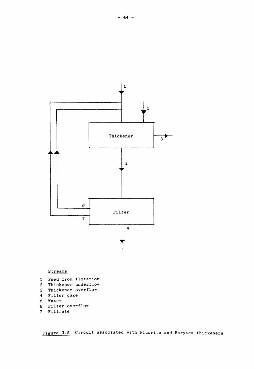
- 44 -

Thickener

"

Filter

Streams

1 Feed from flotation2 Thickener underflow3 Thickener overflow4 Filter cake5 Water6 Filter overflow7 Filtrate

Figure 3.5 Circuit associated with Fluorite and Barytes thickeners

- 45 -

Feed Well

14.92 Metres

Underflow

Figure 3.6 Dimensions of Fluorite thickener

I

- 46 -

0 20 40 60 80 100 120 140 160 180 200 PARTICLE SIZE (MICROS)

Figure 3.7 Size distribution of Fluorite feed

- 47 -

FLUORITE DATA

Depth below % Solidsslurry surface (M)

•1

•3

•5

•7

•9

1-1

1-3

1-5

1-7

1-9

2-1

2-2

2-5

2-1

2-2

2-37

2-3

2-4

2-44

2-74

2-86

3-53

4-05

10-63

r-» v x* * VA ̂ Vrf A UA. *» ± \s 1.^

Diameter (n)

6-1

6-5

6-5

7-0

7-2

7-0

7-0

7-4

7-5

7-5

7-7

22-3

Solids (WT) Mass flow Average Particle

Thickener feed

Thickener underflow

Thickener overflow

Filter overflow

Filter cake

Filtrate

Water sprays

43-85

52-54

1-73

65-05

91-6

3-4

0-0

rate (kg/s)

9-11

8-56

7-03

0-76

4-23

3-81

1-9

Diameter (UL)

54

54

6-6

54

54

22

_

Table 3.8 Fluorite thickener data

- 48 -

Feed Well

7.62 Metres

(0eCOin

•CO

<9 = 6°47'

Underflow

CO

<D

OJ

c

Figure 3.8 Dimensions of Barytes thickener

- 49 -

100

90

70

LU 60CO°£ ena 50

40

30

20

10

0. 20 40 60 80 100 120 140 PARTICLE SIZE (MICROS)

160 180 200

Figure 3.9 Size distribution of Barytes feed

- 50 -

BARYTES DATA

% Solids (WT) Mass flow Average Particle

Thickener feed

Thickener underflow

Thickener overflow

Filter overflow

Filter coke

Filtrate

Water sprays

42-17

52-44

•2

58-22

90-193

2-197

0-0

rate (kg/s)

3-039

3-9

•29

1-275

1-417

1-209

•668

Diameter (ju)

8-6

26-0

6-4

28-5

-

19-5

—

Table 3.9 Barytes thickener data

- 51 -

6

Thickener

Splitter

8

Filter

Streams1 Feed from flotation2 Thickener underflow3 Thickener overflow4 Filter feed5 Filter cake6 Water7 Splitter overflow8 Filter overflow9 Filtrate

Figure 3.10 Circuit associated with Galena thickener

- 52 -

Feed Well

7.1 Metresoe

Underflow

Figure 3.11 Dimensions of Galena Thickener

- 53 -

0 20 40 60 80 100 120 140 160 180 200 PARTICLE SIZE (MICROS)

Figure 3.12 Size distribution of Galena feed

- 54 -

GALENA DATA

Depth below slurry surface (M)

•1

•3

•5

•7

•9

1-1

1-3

1-4

1-5

% Solids (WT)

3-58

10-3

12-42

13-3316-0

15-55

15-7

15-85

15-9

Average Particle Diameter (u)

8-4

10-4

11-2

12-1

13-2

14-1

15-1

13-7

15-1

Thickener overflow

Thickener feed

Thickener underflow

Splitter overflow

Filter feed

Filter overflow

Filter coke

Filtrate

Water sprays

% Solids (WT)

•3

12-7

75-611

74-89

75-626

76-31

90-886

•17

Mass flow Average Particlerate (kg/s)

1-35

•85

5-615

•12

5-495

5-31

•114

•071

•614

Diameter (ju)7-7

15-3

-

32-5

33-5

39-0

-

-

_

Table 3.10 Galena thickener data

- 55 -

CHAPTER FOUR

A NUMERICAL MODEL FOR

NON — FLOCCULATED BATCH SEDIMENTATION

- 56 -

4.1 Introduction

The movement of participates in a host fluid, due to the difference in

particulate and fluid densities, is essentially a transient one

dimensional multiphase problem. Each solid phase being distinct via its

density and/or its size and shape.

When non flocculated particulates settle in a fluid two regions are

observed, see Figure 4.1, these are;

a) Free settling region

b) Sediment region.

The free settling region consists of particles not in contact with other

particles. For a polydisperse suspension this region will contain

distinct zones, see Davies (1985). The lowest zone just above the

sediment containing all particle phases at their initial concentrations,

with each successive zone above containing one fewer phase than the zone

below (ie. fastest settling phase). The sediment region for non-

flocculated slurries will consist of an incompressible packed structure

of particulates. The proposed numerical model makes the following

assumptions:

1) The slurry container has uniform cross sectional area.

2) The flow is vertical and horizontally uniform (i.e. negligible wall

effects).

3) Forces that can act on the solid particles are gravity (allowing for

buoyancy), drag due to the relative motion of the liquid and other

particle phases (particle collisions). Also for flocculated

material a compressive resistance is present due to floe collapse in

the sediment, see chapter six.

- 57 -

Free Settling

Incompressible sediment

Figure 4.1 Non Flocculated Settling Regions

- 58 -

4) The slurry is treated as a continuum; that is continuous solid and

liquid phases that interact with each other.

5) Isothermal conditions are present. Therefore an energy balance is

not required.

The problem consists of a set of moving boundaries one for each solid

phase and one for the build up of the sediment. The following model

predicts concentrations and velocities in the free settling region and

also predicts the build up of the sediment region.

4.2 Governing Equations

The differential equations governing the conservation of mass and

momentum for each solid phase and the equations for the fluid phase are

written in an Eulerian plane of reference. Because of the nature of

this particular problem it is essential that each solid phase be

represented by a continuity and momentum equation. The forces acting on

the solids in an element of thickness dy are:

Drag forcesBuoyancy force

Corapressive force

tdy

i

t (flocculated materialonly)

IGravity force

The corapressive force is the solids pressure term which becomes dominant

in the sediment region for flocculated slurries, see chapter six. The

movement of the fluid phase is essentially due to the movement of

solids. Therefore in the volume dy fluid is displaced due to the move­

ment of particulates. This movement of the fluid phase can be described

by an overall continuity equation, see equation 4.11. This eliminates

the need to solve a fluid phase momentum equation, see Appendix.

- 59 -

4.2.1 Solid phase continuity

Associated with each solids phase is a continuity equation. This

equation represents the conservation of mass for the relevant solids

phase.

3(p l S i' H- 3'Pl S i"i' . o 1-1..NSOL (4.1)at ay

4.2.2 Solid phase momentum

The conservation of momentum for each solid phase is given by the

following equation:

NSOL

< S ip iU i> + - < s iPi u i u i) =

i-l.-NSOL (4.2)

The two terms on the L.H.S. represent the transient and convection terms

respectively. The first term on the R.H.S. represents the fluid

particle interaction. This is based on expressions used by Gidaspow

(1985), where for flow in the free settling region the interaction term

is :

3 (43a)

4 (d)

and for flow within the packed structure of the sediment

FD - 150(1 "F)s i af + i- (4 3b)

- 60 -

where H is the hindered settling effect, due to the presence of other

particles, based on the Barnea (1973) correlation

H = (1 + (1-F) 1 / 3 ) exp 1 (4.4)

The drag coefficient CD is given by the Schiller expression

24 CD = — (1 + 0-15 Re 0 - 687 ) (4.5)

where the Reynolds number is

Re - dfl »f»™l» F . (4.6) "f

The second term represents the particle-particle interaction due to

collisions. The interaction coefficient KJJ is given by the Nakamura

(1976) expression:

f «1J(1*«1J) lu.-UI ,4.7)

The final term represents the force due to gravity and buoyancy acting

on the particles. The mixture density term is simply given by:

NSOL

Pm = FPf + } Pi s i (4.8)

4.2.3 Concentration Balance

The volume fractions are related via the following equation:

NSOL

F + 5 S A = 1 (4.9)

1 = 1

where F is the fluid volume fraction. This equation states that only

- 61 -

solid phases and the fluid are present in the system

4.2.4 Total Volumetric Balance.

The continuity equation for the fluid phase is given by

+ 3(PfFV) =Q>(4

at ay

As the fluid and solids are assumed to be incompressible, the density

terms can be eliminated from equations 4.1 and 4.10. The resulting

equations are for volume conservation. These equations can be combined

to give the total volumetric balance equation:

NSOL

4.2.5 Boundary Conditions

Two main boundaries exist, these are at the top of the slurry and at the

base of the vessel. The velocities at these boundaries are set to zero.

As mentioned earlier other boundaries exist in the slurry (i.e. the

sediment-free settling region interface and the interfaces for each

solid phase in the free settling region) these will be discussed in the

solution procedure, see section 4.5.

4.3 Discretised equations

The vessel is divided into a number of control volumes each of top and

bottom area equal to that of the vessel base, and of height Ay, see

Figure 4.2. Each of the governing equations are discretised using the

fully implicit scheme and finite difference techniques as described by

Patankar (1980).

- 62 -

-*-

S,F,y and p at scalar nodes

U and V located at velocity nodes

Scalar control volume Scalar Nodes

Velocity control volumes X Velocity Nodes

Figure 4.2 Control Volume Specification

- 63 -

The use of a staggered grid, where velocities are located at the

interface between scalar cells, eliminates difficulties associated with

first order derivatives. The upwind scheme is used as an approximation

for first order derivatives, this states that the value of a dependent

variable at an interface is equal to the value of that variable at the

grid point on the upwind side of the face.

Consider a typical grid point, see Figure 4.3, the discretised equation

for the dependent variable o> at this point can be represented by:

= AN<J>N + AS0S + b (4.12)

where 4>p N g is the dependent variable at the centre, North and South

cells respectively. AN and AS are inflow contribution coefficients

and AP is the outflow contribution coefficient. b represents the

source term.

4.3.1 Solid Phase Continuity

The continuity equation (4.1) is integrated over the scalar control

volume and time. Therefore, referring to Figure 4.3 as scalar control

volumes then the integration gives:

rn rt+At 30 . rt+At rtt A (q.TTMPi I f 8S i dtdy + Pi 8 (b i U i'dydt = 0 (4.13)

Js Jt - Jt Js

which discretises to an equation given by (4.12) where <t> is solids

concentration S and:

- 64 -

Ayn+

Ayn

Ays+

ir w

N

• S

n A

Figure 4.3 Typical Control Volume

- 65 -

AN = I-U.OB (4.13a)

AS = I US ,OJ (4.13b)

= 7? + IUn ,OH + I-U^.OJ (4.13c) At P s

b = SOLD (4.13d) p

where each of the above variables is for phase i

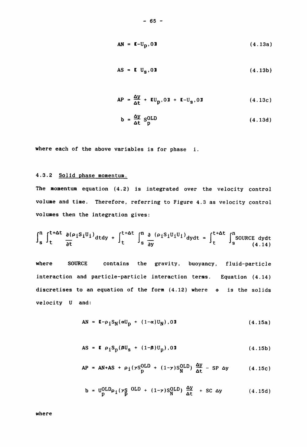
4.3.2 Solid phase momentum.

The momentum equation (4.2) is integrated over the velocity control

volume and time. Therefore, referring to Figure 4.3 as velocity control

volumes then the integration gives:

r rAt a «>is iui>dtdy * rAt rJ s J t J ^ J s dydt

ay

where SOURCE contains the gravity, buoyancy, fluid-particle

interaction and particle-particle interaction terms. Equation (4.14)

discretises to an equation of the form (4.12) where <j> is the solids

velocity U and:

AN = I-P S(«U + (1-«)U),01 (4.15a)

AS = I Pi Sp (PUs + (l-3)Up ),OJ (4.15b)

AP = AN^AS + Pi(7SOLD + (1 _y)sOLD) Z _ sp Ay (4.15c)

b = U°LDp.( 7S OLD + (!_7 ) SOLD) £* + SC Ay (4.15d) p l p N A ^

where

- 66 -

(4.15e)

3 = s+ (4.15f)

y = " • (4.isg)

(Note: That 4.15c is valid due to the application of continuity, see

Patankar (1980)).

The source term contributions SP and SC are given by:

NSOL

SP = - FD - J Kij (4.15h)

J-l

NSOL

SC = FD Vp + J KijUj - S INT

J-l

Where FQ, KJJ and pm are given by equations (4.3), (4.7) and (4.8)

and the concentration values in these expressions, which are at velocity

nodes, are estimated via

SINT = < ySp + (l-r)SN ) (4.15J)

where y is given by equation (4.15g).

4.3.3 Concentration Balance.

The discretised form for this simple relationship is:

N

F + (S d )p = 1. (4.16)

- 67 -

4.3.4 Total Volumetric Balance.

Equation (4.11) is integrated over the scalar control volume. Therefore

referring to Figure 4.3 as scalar control volumes then the integration

gives:

NSOL

f l^'dy + 2 [n li!i^'dy = 0 (4.17)

which discretises to an equation of the form (4.12) where <D is the

fluid velocity V and:

AN = 0.0 (4.18a)

AS = 0.0 (4.18b)

FN if b < 0.0AP = (4.18c)

Fp if b ^ 0.0

NSOLb = ^ {l-(S i ) N (U i ) p ,011 - MSjJp.dJiJp.Ol] (4.18d)

(Note that the values at the south face will already balance as the

equations are solved from the base upwards, see solution procedure).

4.4 Incorporating Packing Theory

As particles reach the base of the vessel they will settle and pack to

form the sediment, which for non-flocculated material will be

incompressible. Due to a size distribution being present the concen­

tration of the packing will depend on what solid phases are present.

- 68 -

4.4.1 Packing Model

During the last few years Ouchiyama (1980,1981,1984,1986) and Cross

(1985) have developed a procedure for predicting the packing voidage of

particulate size distributions. This model is used in the present study

to predict the volume of solids, when treated as a dense packing, in the

scalar control volume being packed.

Suppose that vc^i^ * s tne s Pace allocated to each particle of size

d| in the packed sediment. Then the total volume taking into account

macropores, see Ouchiyama (1986), would be:

VT = max Vc (d i ) N f^) 1 < P < NSOL (4.19) p L

where N and f(d^) are the total number of particles present and the

number fraction of size d^ in a packing consisting of phases 1 to

P. Also phases 1 to NSOL represent the largest to the smallest

particles respectively.

The main difficulty in solving for V-p is the calculation of Vc (d^).

To estimate this value the following assumptions are made:-

a) Each particle is a sphere.

b) Each particle is surrounded by particles of average diameter d,

where:

P

d = dif(di) (4.20)

c) A shell d/2 is imposed over the surface of each particle.

\

- 69 -

d) The number of notional volumes (particle plus shell) which share the

shell space is independent of di.

Although the assumption of sphericity has been made, the model is not

restricted to spherical particles, see Cross (1985). Figure 4.4

illustrates the model with respect to a particle of size di.

The volume of the notional shell that can be shared amongst other shells

is:

VM (<*i) = *? i ~ d) 3 ] (4.21)

where:-

if > d

d =

0 if

If n other notional volumes share VM (di) then the volume of space

allocated to a particle of diameter di is:

VC< d i> - R « (4.22)n

also the volume of solids in Vc (di) is

where EM (di) is the voidage of the shell

The void volume of the shell is given by

n(4.23)

\dj - if- d 3 fl- | —^ ] (4.24)

12 1 I 8 d . +d J

- 70 -

Figure 4.4 Packing Model

- 71 -

where C(dj) is the coordination number of a sphere,

C(di) = [7 - 8E(di)] (4.25) 13 I 2d J

and E(di ) is the voidage of a packing consisting of particles of size

dj only, see Ouchiyama (1980).

The total solids volume in phases 1 to P is given by:

Vs = > o| dj N f(di) (4.26)

and

vs = v ( d ) N

Using the above equations the volume of solids, when treated as a dense

packing, in the cell being packed is calculated as follows.

1) Given size fractions d^ and voidages E(d^) and solids

concentrations in cell being packed S^ then evaluate number

fractions f (d^) .

2) Using equation (4.20) evaluate d.

3) Using equations (4.21) and (4.24) evaluate EM (d i ).

4) Use equations (4.23), (4.26) and (4.27) to evaluate n.

5) Use equations (4.19) and (4.22) to evaluate VT .

The calculated value of VT can be compared with the cell volume Ay

to see if the cell is fully packed with particulates .

- 72 -

4.4.2 Further densification of sediment

For non flocculated slurry's the sediment predicted, see section 4.4.1,

will contain pores in which small particles may still penetrate and

pack, see Kitchener (1977). In order to determine whether or not small

particles may penetrate the packed structure forming the sediment an

estimate of the size of the open pores is required.

An estimate which is used in this study is the hydraulic diameter, see

Gray (1968). This is obtained by assuming the sediment to consist of a

set of column channels of constant hydraulic diameter given by:

_ ____Volume of voids______H = Surface area wetted by fluid (4.28a)

where:

Volume of voids = FAy (4.28b)

NSOLr

Surface area wetted by fluid = 6Ay )Sj/d^ (4.28c)

Therefore given the concentrations in the sediment an estimate of the

pore size is given by:

3 NSOL<V

dI 2

If particles exist whose diameter is less than DH then these particles

will penetrate into the sediment increasing the overall solids

- 73 -

concentration which will in turn decrease the hydraulic diameter. This

process will continue until the solids diameter is greater than the

hydraulic diameter. Also the movement of small particulates into a

packed porous structure is governed by a modified form of the Ergun

equation representing the fluid particle interaction term, see equation

(4.3b).

4.5 Solution procedure

The dependent variables Si, U A (i = l...NSOL), F and V are to be

solved at different locations throughout the vessel over time, see

Figures (4.8). The equations to be solved at each time step are

non-linear and highly coupled. Therefore, the finite difference

equations (4.12) are solved using an iterative procedure. These finite

difference equations are solved at each iteration in the following

order:

1) Solid phase momentum and continuity for U^ and S^

respectively i=l...,NSOL.

2) Concentration balance for F.

3) Total volumetric balance for V.

At the next iteration the new value of the fluid velocity, V, will

effect the movement of the particulates as it is incorporated into the

momentum equation of each solid phase. This in turn will give rise to

new values of S^, Uj and F until convergence has been obtained.

As the variables to be solved are volume fractions and velocities the

Jacobi point-by-point iterative procedure is used, see Markatos (1983).

Therefore Op is solved from the base upwards for all nodes in the

vessel, via:

- 74 -

Op = (AN0N + ASOS + b)/AP (4.29)

where the values for o^ and 0S are from the previous iteration

sweep.

The fluid volume fractions are calculated using equation (4.16) where

the solid volume fractions are those at the present iteration. The

fluid velocities are calculated using equations (4.18) together with

(4.12) where the solid volume fractions and velocities in b, equation

(4.18d), are those at the present iteration. As the solution procedure

is from the base upwards then, when solving for V, the flow across the

south face of each scalar control volume will balance and the solution

procedure only needs to balance the flow across the north face. This

gives rise to equations (4.18).

Each variable is checked for C9nvergence at the end of each iteration.

This is achieved by noting the maximum relative error associated with

each variable (i.e. RESID) and comparing it with a given tolerance (i.e.

TOL). The relative error at each node for variable o is obtained,

via:

RESID = I* - 0 I/M (4.30)

where o* is the value of variable o at the previous iteration.

The movement of each solid phase boundary in the free settling zone is

monitored by noting what scalar control volume the boundary is in

initially (i.e. top cell). At the end of each time step the location of

this boundary in the cell is calculated, via:

- 75 -

AyT = AyT* - I-Us,OJAt (4.31)

where AyT and AyT are the boundary positions in the cell at the

present and previous time steps respectively. Us is the velocity at

the south face, see figure 4.6.

tI

Figure 4.6 The Boundary Cell

The concentration in the boundry cell for phase i is noted when

U< for that phase becomes negative (i.e. downward flow). This

concentration is assumed to be uniform throughout the cell. After

intervals of time the cell will contain a lesser amount of phase i due

to the movement of this phase out of the cell. The concentration of

phase i between the boundary b and the interface S will be

but the concentration at P will be for the whole cell. When solving

- 76 -

for Us and the concentration at node S it is the value of STB which

is used for cell P, not the concentration stored and calculated at P.

This avoids a concentration gradient forming due to ignoring the

presence of the boundary. When AyT becomes negative then the boundary

has left the cell and entered the cell below. The concentration in the

new boundary cell is adjusted to represent the new boundary position and

value of

The flow of solids into the cell being packed is modelled in a manner

similar to the above procedures, see Figure 4.7.

Figure 4.7 The sediment cell

The concentration between the boundary b and cell interface n will

be the initial concentration SBB . This is the value used for cell P

when calculating Up and concentrations at node N. This once again

- 77 -

C START

Input data

Update TIME for next time step

(TIME=TIME+ TSTEP) . Calculate concentrations

and velocities at this point in time.

ICheck cell being packed

(i.e. IYPAK) for sediment volume

IUpdate values for the dependent

variables at previous time step.

NO

YES

STOP

Figure (4.8b)

Figure (4.8c)

Figure 4.8a Overall solution procedure

- 78 -

Start of iteration

sweep IPHASE=IPHASE+1

••

Update previous

iteration values

"

IS

IPHASE=NSOL+1

Calculate fluid

phase concentrations

and velocities

TCalculate relative

errors between present

and previous values

YES

Calculate solid

phase concentrations

for phase IPHASE

Calculate solid

phase velocities

for phase IPHASE

NO

Figure 4.8b Iteration cycle

- 79 -

Calculate packing

Volume VT in IYPAK

NO

I YPAK= IYPAK+1

1

TIM

Using

recalc

IYPAK

V

*

YES

TIME = TIME - TSTEP

iTIME = TIME + TSTEP/1000

Using calculated velocitiesrecalculate concentrations inIYPAK at this point in time

Calculate packing

volume VT in IYPAK

NO

YES

Insert excess

solids into IYPAK+1

Figure 4.8c Packing cycle

- 80 -

avoids a concentration gradient forming due to ignoring the sediment

boundary. When the cell becomes packed the concentrations are adjusted

so that

VT = Ay. (4.32)

and the excess solids are inserted into the cell above. If the

hydraulic diameter, see section (4.4.2), for the packed cell is greater

than the diameter of the smaller particles then these may still flow

into the cell until the hydraulic diameter becomes to small.

4.6 Comparisons with Holdich data

Concentration profiles have been obtained by Holdich, see Holdich

(1983), for Ballontini undergoing settlement in water. The experimental

procedure uses electrical conductivity techniques and a perspex tube of

height 48cm and internal diameter 7-7cm. Unfortunately no size

distribution was obtained for the Ballontini, but the material was

carefully sieved between 45a and 75^ and a mean particle diameter of 55/u

was observed (by Microscopy). Data was gathered for seven experiments

where the initial solids concentrations are 0-1, 0-15, 0-2, 0-25, 0-3,

0-35 and 0-4.

For this study it is essential to obtain a size distribution so that the

multiphase effect can be observed. To enable this a Schumann

distribution, see Schumann (1940), is used. This is given by:

•GO"(4.33)

where Y is the cumulative fraction undersize represented by all

- 81 -

particles of size between On and Xa. K is the maximum particle size

for which Y is unity and M is a constant near unity. The Ballontini

is broken down into 2,3 and 5 phases by dividing the size range into

equal parts. The concentrations for each phase is obtained by letting

M equal 0-8, 1-3 and 1-55 for 2,3 and 5 phases respectively, see tables

4.1, 4.2 and 4.3.

The density of the Ballontini used was calculated using a density bottle

to be 2865 Kg/m 3 .

Comparisons between the experimental data obtained by Holdich and the

model predictions at 1,2,3 and 5 phases are given in Figures 4-9-4-15.

It can be seen that particle segregation occurs in all experiments due

to the concentration gradients observed. The degree of segregation is

higher at lower concentrations although at high concentrations it is

still present. This obviously necessitates the use of multiphase

techniques as the one phase predictions fail to predict the general

settling profile. Although the model predicts the profiles better by

increasing the number of phases used, it seems to underestimate

velocities at 0-1 solids concentration and overestimates at 0-35 and

0-4. This is probably due to:

1) Use of the Schumann distribution to obtain initial phase

concentrations.

2) Observed mean diameter of 55w being in error.

3) Errors in experimental data.

4) The empirical correlations used for fluid-particle and

particle-particle interactions being in error at these

concentrations.

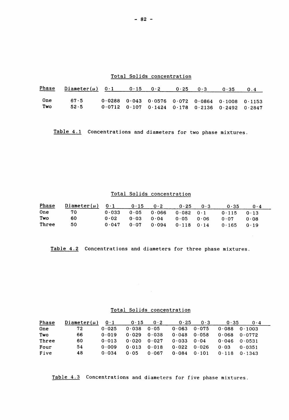
- 82 -

Total Solids concentration

Phase Diameter()u) 0-1

One Two

67-5 52-5

0-15 0-2 0-25 0-3 0-35 0.4

0-0288 0-043 0-0576 0-072 0-0864 0-1008 0-1153 0-0712 0-107 0-1424 0-178 0-2136 0-2492 0-2847

Table 4.1 Concentrations and diameters for two phase mixtures.

Phase One Two Three

Diameter(fj) 70 60 50

Total Solids concentration

0-1 0-15 0-2 0-25 0-3 0-35 0-40-0330-02

0-047

0-050-030-07

0-0660-04

0-094

0-0820-05

0-118

0-10-060-14

0-1150-07

0-165

0-130-080-19

Table 4.2 Concentrations and diameters for three phase mixtures.

Total Solids concentration

PhaseOneTwoThreeFourFive

Diameter(n 72 66 60 54 48

0-10-0250-0190-0130-0090-034

00000

0-15•038•029•020•013•05

00000

0-2•05•038•027•018•067

00000

0-25•063•048•033•022•084

00000

0-3•075•058•04•026•101

0-0-0-0-0-

0-35088 0068 0046 003 0118 0

0-4•1003•0772•0531•0351•1343

Table 4.3 Concentrations and diameters for five phase mixtures.

- 83 -

One phase

O.M

Two phases

T o'.a n oa CONCENrRAflON

Three phases Five phases

Expe r imen t a1 Da ta

• Initial concentrations

i 36 sees

4- 1 run 12 sees

x 2 mins

Figure 4.9 Comparisons with Holdich data at 90% porosity

- 84 -

<J-

8

.00 O.M O.tt O.M O.U 0.40 0.4i CONCENTRATION

o.oo O.M 6.1* O.H O.it 0.14 0.4* O.SS CONCENTRATION

One phase Two phases

0.00 O.M ft.lt O.H O.U 0.40 0.4tCONCCNTRATION

0.00 O.M O.;f O.U O.U 0.44 fl.»« O.U CONCENTRATION

Three phases Five phases

Experimental data

• Initial concentrations

A 1 min

+ 2 mins

x 3 mins

Figure 4.10 Comparisons with Holdich data at 85% porosity

- 85 -

Si

O.U ' 0,» 0.«9 ' O.*tUSO »,M 0.1*

One phase

O.OB o.tt M O.ttcoNttwrRArroN

Two phases

««

M

Three phases

</,? 8*

.00

Experimental Data

• Initial concentrations

A 36 sees

+ 2 mins

x 4 rains

. .CONCtNTRATION

Five phases

O.M

Figure 4.11 Comparisons with Holdich data at 80% porosity

- 86 -

5

5

oo o.o* o.t* fl.u o,« o.ta o.** ».» CONCENTRATION

One phase Two phases

4.M C.H ».H O.U 0.40

Three phases Five phases

Experimental data

• Initial concentrations

A 36 sees

+ 1 min 12 sees

x 2 mins

$ 4 mins

Figure 4.12 Comparison with Holdich data at 75% porosity

- 87 -

£*5®*A

O'.U

One phase

o.t» t.u o.ii ».*o o.a

Two phases

o.i* o.w o.«o o'.a CONCENTRAfiON

Three phases

1.00 ' O.M O.H O.M 0.1( 0.40 CONCENTRATION

0.4* 0.3*

Five phases

E xp e r i me n t a1 da t a

• Initial concentrations

A 30 sees

+ 2 mins

x 4 mins

^ 5 rains

Figure 4.13 Comparisons with Holdich data at 70%

- 88 -

a

8

,00 0.01 0.11 O.M 0.3S 0.40 0.41 0.31 CONCENTRATION

.00

One phase

0.01 0.11 O.M o.a 0.40 o.a CONCENTRATION

o'.s»

Two phases

«J

3'

5.

o-

8

0.00 0.01 0.11 O.M O.JS 0.10 O.a O.MCONCENTRATION

Three phases

LOO O.M 0.11 O.M O.M CONCENT

Five phases

0.40 0.41 0.31 TRATION

Experimental data

• Initial concentrations

i 1 min

+ 2 mins

x 4 mins

$ 6 mins

Figure 4.14 Comparison with Holdich data at 65% porosity

- 89 -

t

TS^ o.rt

One phase

S5*1

1.00 o.it a.u o.« t.40 CONCEHTRATION

Two phases

o.*oCONCENrRATION

O.M

Three phases Five phases

Experimental data

• Initial concentrations

1 30 sees

+ 2 mins

x 4 mins

4 5 mins

Figure 4.15 Comparison with Holdich data at 60% porosity

- 90 -

The concentrations observed in the sediment ranged from 0-58 for the 60%

porosity experiment to 0-5 for the 90% porosity experiment. This is due

to variation in the packing arrangement where the 60* porosity

experiment settled much slower with a more ordered packing structure

being observed. For this set of data the packing model used values of

E(dj) to be the observed maximum concentration. In all cases the

calculated hydraulic diameter was less than the smallest particle phase

size, thus prohibiting particle movement into the sediment.

4.7 Comparisons with Experimental Data

Experimental data has been gathered for a number of one, two and three

phase particulate mixtures undergoing batch sedimentation, see chapter

two. These experiments measured the changes in slurry density above a

certain height during the settlement of an initially uniform suspension.

The above numerical model predicts concentrations at different points

throughout a suspension. From these concentration profiles the slurry

density above a transducer is calculated by:

NYPh = I Pm *Vi < 4 - 34 )

i=T

where T is the cell containing the transducer and NY is the top

cell, h is the height of mixture above the transducer and Ay^ is the

volume of cell i containing a particulate mixture of density pm , see

equation (4.8). The volume Ay^ is not the volume of the cell

containing the transducer but the volume between the transducer and the

north face of the cell. Using the numerical model and equation (4.34)

comparisons between density profiles obtained in chapter two and those

predicted using the proposed model can be made.

- 91 -

For all the numerical simulations the values of the collision coeffic­

ients <xjj and e.^ are taken as one, which represents head on elastic

conditions between each of the particulate phases, see Nakamura (1976).

The voidage of each phase when packed alone, E(d^), is taken as 0-38

for Glass and Copper spheres which represents a random packing

structure. The value of E(d i ) for quartz, which is angular, is taken

as 0-4, see Cross (1985). The sediment is checked for further

compaction by calculating the hydraulic diameter.

Also compared with the experimental data is the model by Selim (1983),

see chapter one, which presents the state of the art at the present

time. The following plots represent these comparisons as well as

concentration profiles of each particulate phase predicted by the

proposed model.

4.7.1 One phase comparisons

For solid particulates represented by a unique size, density and shape

factor the numerical model is used where the collision term KJJ is

zero and further densification of the sediment is ignored due to the

presence of only one solid phase.

Comparisons of both the Selim model and the proposed model with

experimental data have been made, see figures (4.16-4.26). The

outstanding feature in all these comparisons is the closer fit to the

experimental data for the proposed model. The general trend seems to be

that the Selim model over predicts the settling velocity of the

particulates. This in turn gives greater density changes over time than

those observed. The greater deviations between the proposed model and

the experimental data during the later part of the experiments is due to

segregation effects. This is because the particle size used to

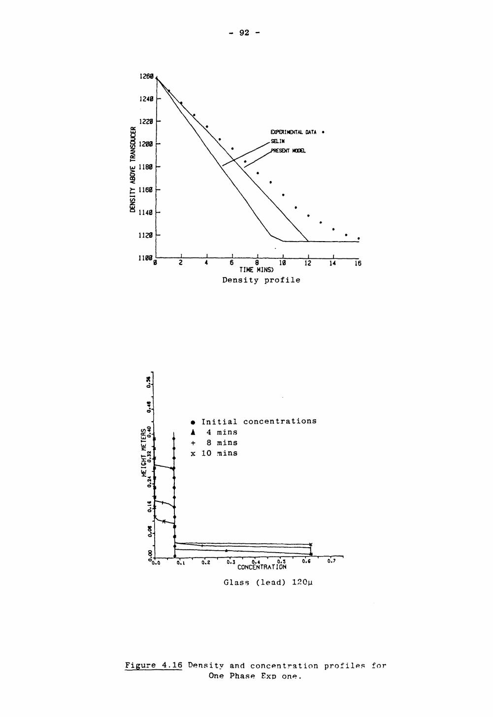
- 92 -

1260

1240

1140 -

1120 -

1100

EXPERDOfMl. DATA •saiN

SENT MODEL

I 2i

4i

6 81

10 12 14 IfTIME MINS)

Density profile

<c^-

UJ .

s

0.0

• Initial concentrations i 4 mins + 8 mins x 10 mins

0.2 0.3 0.4 0.3 CONCENTRATION

Glass (lead)

0.6 0.7

Figure 4.16 Density and concentration profiles forOne Phase Exp one.

- 93 -

1268,

1240

1220

1200

1180

fc 1160

° 1140

1120

1100

>

0 20 40

EXPERIMENTAL DATA •saiNPRESENT MOOEL

1 1 1 1 1 1 1 160 80 100 120

TIME (SECS)

Density profile

140 160 180

• Initial concentrationsA 30 sees+ 90 seesx 120 sees

o.z 0.3 0.4 O.SCONCENTRATION

0.6 0.7

Glass (lead) 275u

Figure 4.17 Density and concentration profiles forOne phase Exp two.

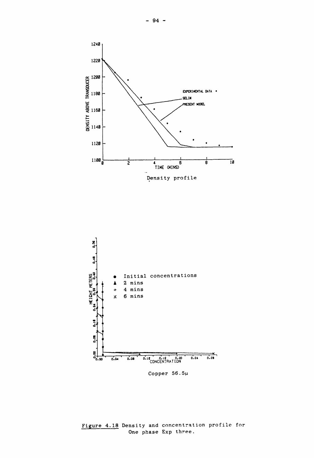
- 94 -

1240

1220

eg 1200 o

1 1180

ui

1 1160

in5 1140

1120

11000

EXPERIMENTAL DATA

sainMODEL

4 6TIME (MINS)

Density profile

10

B3J • Initial concentrationsA 2 mins+ 4 minsx 6 mins

0.24

Copper 56.5|a

Figure 4.18 Density and concentration profile forOne phase Exp three.

- 95 -

1260,

1240

1220

1200

1180

1160

1140

1120

1100 0

EXPER»€NTAL DATA •

SELIN PRESENT MQOQ.

20 40 60TIME (SECS)

Density profile

100 120

iMt-"5°

0.0

• Initial concentrations i 30 sees + 60 sees x 90 sees

o.i (T.Z 0.3 0.4 O.SCONCENTRAT[ON

0.6 0.7

Glass (lead) 275u

Figure 4.19 Density and concentration profiles forOne phase Exp four.

- 96 -

5

1340 1320'

1300

1280

1260

I 1240Q£

ui 1220

< 1200>-5 H80z^ 1160

1140

1120

1100

EXPERIMENTAL DATA •

saiNPRESENT MOOEL

0 20 40

5°

80.0 0.1

60 80 TIME (SECS)

100 .'.23 140

Density profile

• Initial concentrations A 45 sees + 90 sees x 135 sees

0.2 0.3 0.4 0.3CONCENTRATION

0.6 0.7

Glass (lead) 275|a

Figure 4.20 Density and concentration profiles for .._ One phase Exp five.

- 97 -

1600

EXPERIMENTAL DATA •

sainPRESENT MODEL

20 40 60 80 100 120 140 160 180 TIME (SECS)

Density profile

• Initial concentrations A 45 sees + 90 sees x 150 sees

0.0 0.1 0.2 0.3 0.4 0.3 0.6CONCENTRATION

0.7

Glass (lead) 275|a

Figure 4.21 Density and concentration profiles forOne phase Exp six.

- 98 -

1100,

EXPERIMENTAL DATA •saiMPRESENT WOO.

20 40 60 80 100 120 TIME <SECS)

140 160 180

Density profile

8

• Initial concentrationsA I min+ 2 minsx 3 mins

C>T——i——i——i——r 0.0 0.1 0.2

~i——l——i——i——i——i——i——i——i 0.3 0.4 O.S 0.6 0.7

CONCENTRATION

Glass (lead) 275u

Figure 4.22 Density and concentration profiles forOne phase Exp seven.

- 99 -

1120 -

1100 U

EXPER1HEWTAL OATA •,saix

Hooa

uj 1080

§ £ 1060

° 1040

1020

1000j

\ *^\.

: \\i I i i I r — —10 20 30 40 50 60

TIME (SECS)70

Density profile

• Initial concentrationsi 30 sees-i- 60 seesx 90 sees

0.0 O.t o.* 0.3CONCENTRATION

0.6 0.7

Glass (lead) 76.5u

Figure 4.23 Density and concentration profiles forOne phase Exp eight

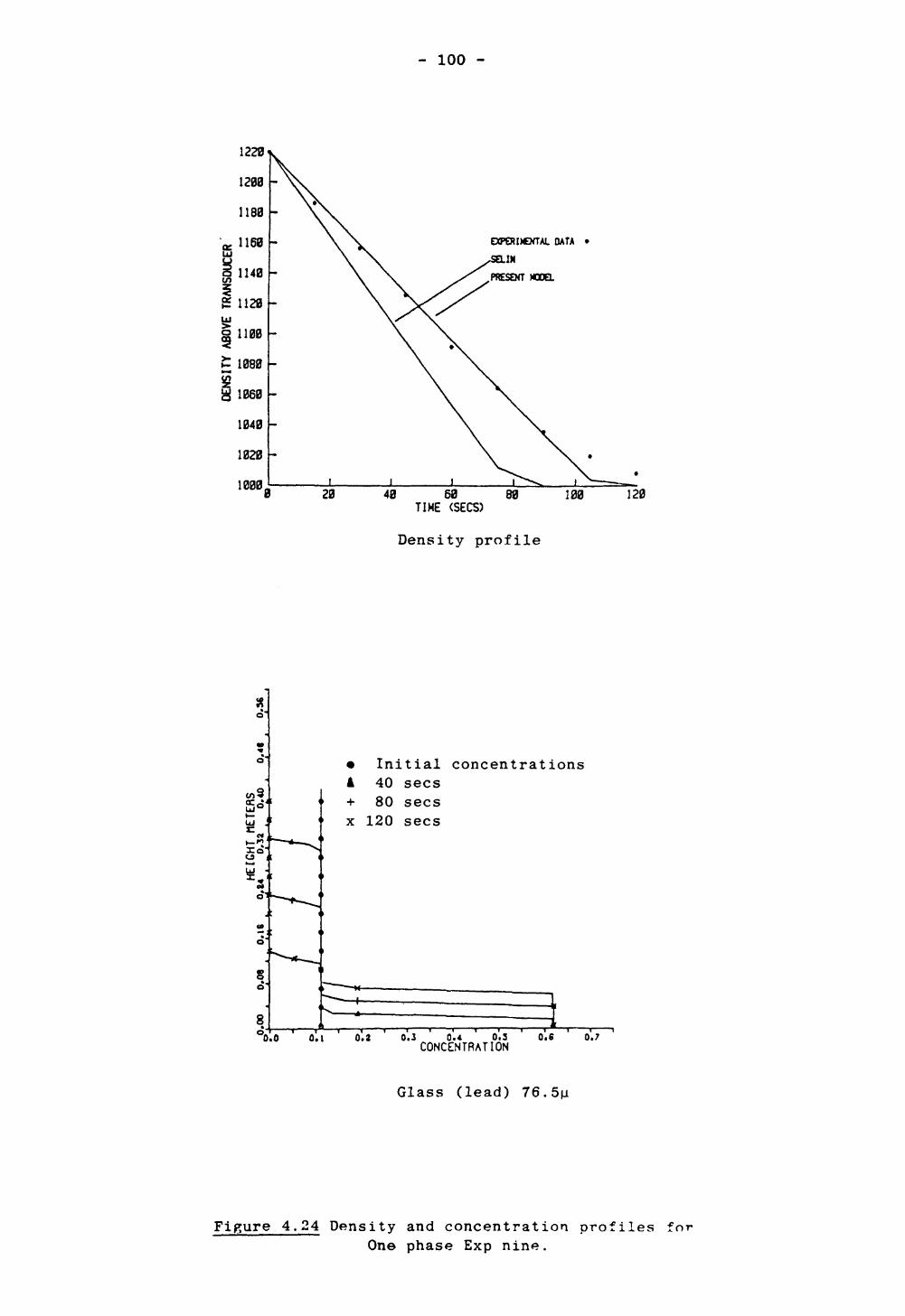
- 100 -

20

EXPERDGtTAL DATA •

IN

PRESENT MODEL

40 60TIME (SECS)

80 100 120

Density profile

KJ •

CJ

5

• Initial concentrations A 40 sees + 80 sees x 120 sees

°0.0 0.1 0.2 0.3 0.4 0.3 0.6CONCENTRATION

0.7

Glass (lead) 76.5u

Figure 4.24 Density and concentration profiles forOne phase Exp nine.

- 101 -

20

EXPERI)€NTAL DATA • SEL1M

MODEL

68 80 100 TIME (SECS)

120 140 160

Density profile

5°5*

8

• Initial concentrations A 40 sees + 90 sees x 150 sees

0.0 0.1 0.2 0.3 0.4 0,3CONCENTRATION

0.6 0.7

Glass (lead) 76.5|u

Figure 4.25 Density and concentration profiles forOne phase Exp ten.

- 102 -

20

EXPERIMENTAL DATA •

SELINPRESENT MOOEL

40 68 80 TIME (SECS)

100

Density profile

120 140

8

• Initial concentrations A 40 sees + 90 sees x 150 sees

0.0 0.1 0.2 0-3 0.4 0.3 0.6 0.7CONCENTRATION

Glass (lead) 220|u

Figure 4.26 Density and concentration profiles forOne phase Exp eleven.

- 103 -

represent the solids phase is the mean aperture size of the sieves used

in obtaining the solid particulates, therefore segregation of partic- ulates will occur due to the size range of particulates present.

As observed in the comparisons with the Holdich data the proposed model

over predicts settling velocity at higher solids concentrations. But

unlike the Holdich comparisons the proposed model still over predicts

settling velocity at low concentrations although to much lesser extent.

This is probably due to the assumptions made about the Holdich data.

4.7.2 Two phase comparisons

A two phase non-flocculated particulate mixture will settle with four distinct zones. These are from the top down:

1) Clear liquid.

2) Slurry containing slowest settling particles only.

3) Slurry containing both particulate phases at their initial concent­

rations.

4) Sediment.

Comparisons between the proposed model, Selim's model and the

experimental data have been made, see figures (4.27-4.35). As with the

one phase comparisons the general trend is the same with the Selim model

over predicting settling velocities leading to greater density changes

than observed. In the comparisons the proposed model restricts

particulate settling to a greater extent than the Selim model, this

leads to a closer fit with the experimental data.

From the concentration plots the build up of the sediment using the

packing model and the formation of a zone containing the slower moving

phase only can be observed. The sediment zone for each experiment will

contain both particulate phases where the predicted solids

- 104 -

TIME <MINS>

Density profile

nS

I

r

• Initial concentrationA 1 fflin+ 3 minex 4 mins• 6 Bins

o.oo t.M o.M o.it o.ic o.»

Copper 56.

O.M

• Initial concentrations A 1 nin•*• 4 mine x 8 nine• 14 mine

Glass (lead) 76.5u

Figure 4.27 Density and concentration profiles forTwo phase Exp one.

- 105 -

1400

EXPERIMENTAL QATA

SELINPRESENT MOOa

11004 5

TIME (KINS)

Density profile

Ri

• Initial concentrations A 30 sees + 60 sees x 90 sees• 120 sees

o

5 i

•.I *.l *.l (.4 *.! 1.1 «.?

• Initial concentrations* 1 min + 2 nins x 5 Bins 4 7 tains

o.no A.M «.«• 0.1* «.i* 8-jo *.u o.a CONCENTRATION

Glass (lead) 302. Copper 56.5

Figure 4.28 Density and concentration profiles forTwo phase Exp two.

- 106 -

1400

EXPERIMENTAL DATA •

IK PRESENT MODEL

6 8 10 12 14 161100

Density profile

• Initial concentrations A 1 min + 2 mine x 3 mins

• Initial concentrations A 3 mins + 6 mins x 9 mins

O.M O.«0 CONCENTRAT ION

O.MCONCENTRArON

Glass (lead) 327. Glass (lead) 120n

Figure 4.29 Density and concentration profiles forTwo phase Exp three.

- 107 -

1300

1000 >

EXPERDCXTAL DATA •

SEL1M

PRESENT MODEL

4 6 TIME (MINS)

Density profile

• Initial concentrations A 2 rains + 4 Bins x 6 mine

"o.oo o.ot o.i* 0.14 o.jf o.te o. CONCENTRATION

*.^*5 e5.

• Initial concentrations A 2 mins + 6 mins x 9 mins

0.00 O.I 0. It O.C4 O.M O.iO 0.4« CONCCNTHAfJON

Glass (soda) 69tt Glass (soda) 41.5u

Figure 4.30 Density and concentration profiles forTwo phase Exp four.

- 108 -

1450

EXPERIMENTAL DATA •SEL1M

PRESENT HOOEL

10 15 20 TIME (MINS)

25 30

Density profile

5o

• Initial concentrations i 1 Din + 2 rains x 3 inins

• Initial concentrations 1 3 mine + 10 mins x 20 fflins

0 .00 O.M I.I« 0.14 O.M 0<«6 CONCCNTftATION

o.a O.M 0.1 «.) 0.4 0.1CONCENTRATION

Quartz 200p Glass (soda) 60n

Figure 4.31 Density and concentration profile forTwo phase Exp five.

- 109 -

1148 -

1120 -

1100

EXPERIMENTAL DATA •

saiMPRESEHT MODEL

1J 2

14

i6 8 10 1.

TIME (MINS)

Density profile

X•i-

• Initial concentrations A 40 sees + 80 sees x 120 sees It

r<j'

"0.00 0.0* ».!« O.tt ' O.X O.tfCONCENTRAT I ON

O.U O.M

• Initial concentrations 1 2 rains + 6 mins x 10 mins

o.t 0.1 0.4 0.9CONCENTRATION

Glass (lead) 275u Glass (lead) 120|j

Figure 4.32 Density and concentration profiles forTwo phase Exp six.

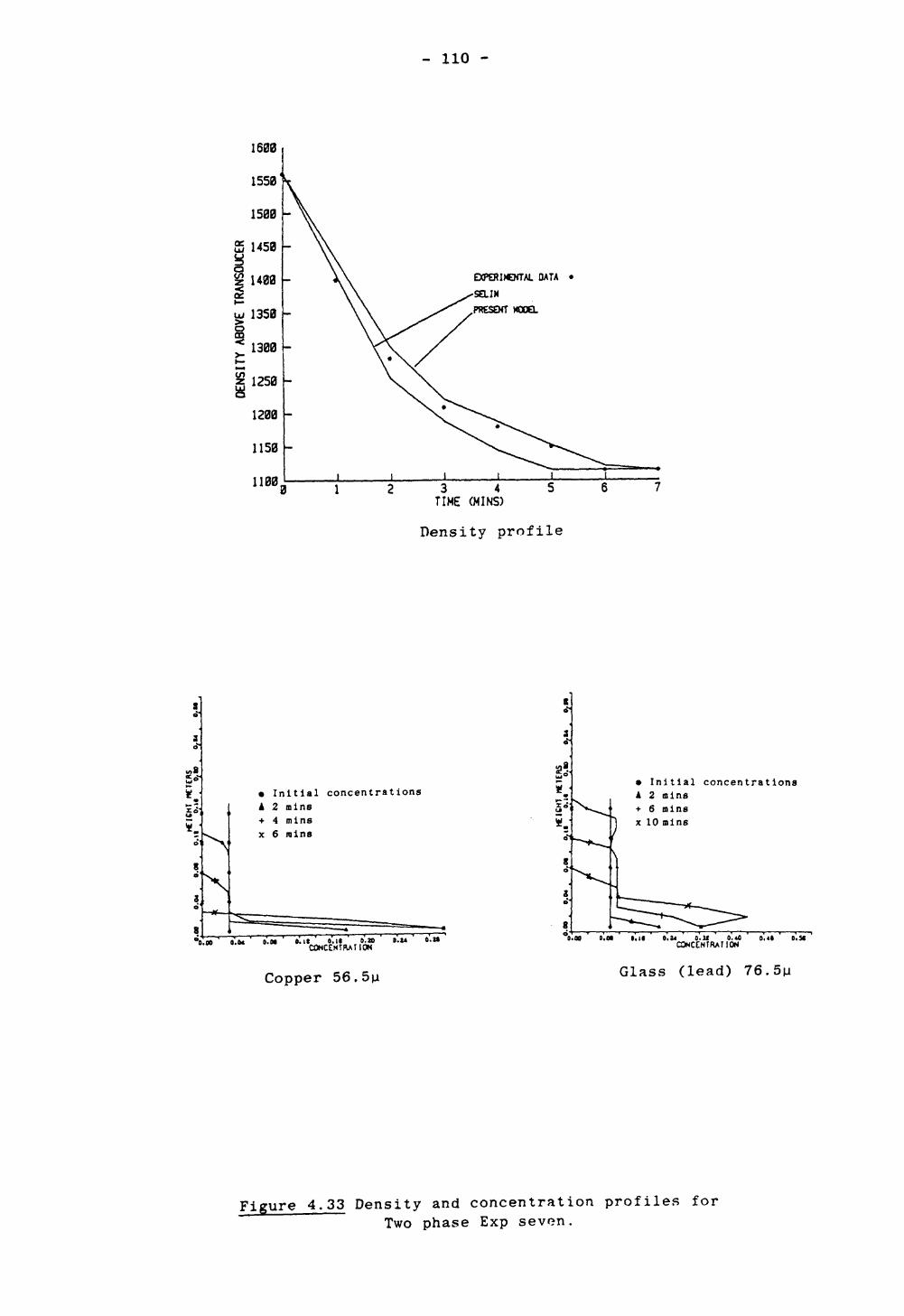
- 110 -

EXPERIMENTAL DATA

sainPRESENT

3 4 TIME (MINS)

Density profile

* -

• Initial concentrations i 2 rains + 4 mins x 6 rains

0.04 O.M O.It O.I* »'.» CONCENTRATION

l.U O.I*

• Initial concentrations A 2 mine + 6 nine x 10 mine

"o.ao o.o* o.ii o.t4 o.itCONCENTRATION

o.x

Copper 56. Glass (lead) 76.

Figure 4.33 Density and concentration profiles forTwo phase Exp sevon.

- Ill -

EXPERIMENTAL DATA •

sawPRESENT MODEL

30 40 TIME 04INS)

50 60 70

Density profile

t

5*5a

• Initial concentrations A 40 sees + 80 sees x 120 sees

a

V. •.• ' *« ' ^c&T^oH

Glass (lead) 302.5n

• Initial concentrations A 2 Bins + 20 Bins x 50 mlns

0,0* .i« e.u ».a «.<a *•*« «.iC9NCCNTRATION

Glass (lead) 41.

Figure 4.34 Density and concentration profiles forTwo phase Exp eight.

- 112 -

1450

EXPERIMENTAL DATA •IX

.PRESENT

1100 6 8 10 12 14 16 18 20 22 TIME (M1NS)

Density profile

• Initial concentration* A 2 mlns + 4 Bins x 6 ain*

•.II 1.OMCCNtRAUCN

Glass (lead) J?20fj

a'. a«• Initial concentrations A 6 mine + 12 mine x 20 mine

0.1 ft.4 0.) O.I 0.'

Glass (lead) 76.5ja

Figure 4.35 Density and concentration profiles forTwo phase Exp nine.

- 113 -

concentrations of the sediment for each experiment are

Experiment Solids concentration Hydraulic diameter

Exp one 0-622 26mi

Exp two 0-639 lOOju

Exp three 0-656 89/u

Exp four 0-624 26^

Exp five 0-686 43/u

Exp six 0-651 82a

Exp seven 0-622 26/u

Exp eight 0-645

Exp nine 0-662

Table 4.4 Sediment concentrations for two phase runs.

Further densification of the sediment can occur in Exp two and Exp eight

as the hydraulic diameter is greater than the diameter of the smallest

particulate phases present in these experiments. Although this does not

occur for Exp eight until all the larger particles have settled because

in the zone where both phases are undergoing settlement at their initial

concentrations the movement of the smaller particles is in the opposite

direction (i.e. against gravity), see figure 4.34. This effect was also

predicted by Selim and is due to the large drag force exerted on the

small particles via the fluid movement. The sediment in Exp two and Exp

eight will continue to be packed with smaller particles occupying the

voids until the sediment solid concentrations are 0-702 and 0-721

respectively.

4.7.3 Three phase comparisons

Three phase non-flocculated particulate mixtures undergoing sediment­

ation will settle with five distinct zones. These are from the top down

- 114 -

1) Clear liquid.

2) Slurry containing slowest settling phase only.

3) Slurry containing the two slower settling phases.

4) Slurry containing all three phases at their initial concentrations

5) Sediment.

Comparisons between Selim's model, the proposed model and the

experimental data for the six three phase experiments have been made,

see figures (4.36-4.41)

Referring to the density profiles the change in gradient of each profile

represents the point at which one of the zones has passed the transducer

so that the change in density is now dependent on the rate of fall of

the next zone. Selim predicts greater velocities for the largest phase

present in each experiment than the proposed model. This will in turn

predict greater concentrations for the phases in the two zones above

which is why the Selim model underpredicts the change in density for Exp

three, Exp four and Exp five. For the other comparisons this has not

occurred to such a degree, if at all. The proposed model predicted the

movement of the slowest phase, in the zone containing all particulate

phases, acting in the same direction as the fluid (i.e. against gravity)

for Exp two, Exp three, Exp four and Exp five. This was also predicted

by the Selim model except for Exp four where the velocity although very

small in magnitude acted in the direction of gravity.

The concentration plots give the formation of the sediment and of the

four zones present in the free settling region over time. The sediment

zone for three phase particulate mixtures will contain three layers

consisting of from the base up:

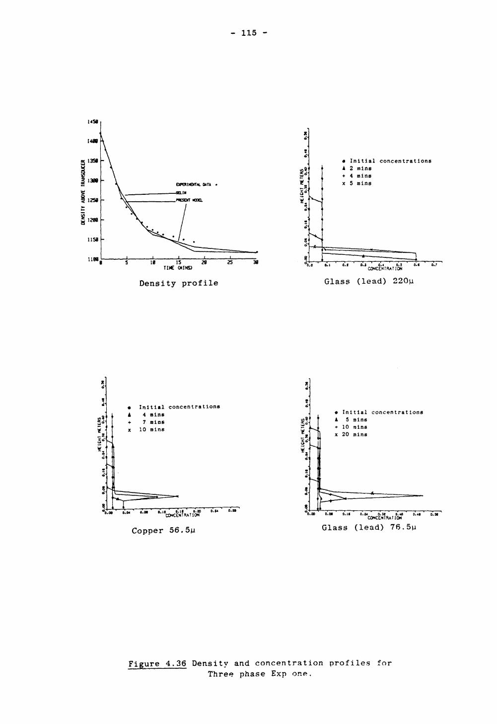
- 115 -

us*

Bf&HOftH. DATA •

4EL1N

10 IS 28 TDC CHINS}

Density profile

25

X a'

•

»95°'

*-;Id'<j5 '3o'

«5-

so"

8

• Initial concentrations

"^^^

^S-* —

A 2 mins+ 4 minsx 5 mins

V- — -, -^^^^^m"0.8 0.1 0.1 6.4 0.3

CONCENTRATION

Glass (lead) 220u

• Initial concentrationsA 4 mins•(• 7 minsx 10 mins *

5^ *,

8

o.it o.il o.aCOKENTRATSON

• Initial concentrations A S mins +• 10 rains x 20 mins

0.00 0.0* O.M O.lt 0.<ACONCENT.RAT i ON o.a

Copper 56. Glass (lead) 76.5|a

Figure 4.36 Density and concentration profilesThree phase Exp one.

:or

- 116 -

UM

1188 is aTIlC WINS)

J

8

• Initial concentrationsA 20 sees+ 40 seesx 60 sees

Density profile

I. (4 ' O'.U ' O-'fi CONCENTRATION

Glass (lead) 462

• Initial concentrations A 1 Bin + 2 Bins z 4 ilns

**

• Initial concentrations A 4 Bins + 10 mins x 15 Bins

M ' ».<

Glass (lead) 200n

O.lt O.KCONCCNTRATION

Glass (lead) 76.

Figure 4.37 Density and concentration profiles forThree phase Exp two.

- 117 -

net

lisa

I10B It IS 2B T1X WINS

Density profile

• Initial concentrations A 40 Sees + 80 sees x 120 sees

0.00 B.M S. If'eoNC&ifnAnW M '•*

Glass (lead) 327.

5• Initial coDcentratioos 1 1 Bin + 2 Bins x 4 Bins

8*1• Initial concentrations 1 4 ains + 10 ains x 20 ains

0.} 1.4 1.3CONCENTRATION

Glass (lead) 200*1 Glass (lead) 76.

Figure 4.38 Density and concentration profiles forThree phase Exp three

- 118 -

CUM

Initial concentrations1 aiin2 rains 4 nine 10 mlns

4 6 8 18 12 TINE WINS)

Density profile

14

Glass (lead) 220n

aa'

s*5*5.

o-

• Initial concentrations* 1 min + 2 mins x 4 mins

10 mins

• Initial concentrations A 1 nin + 2 Dins x 4 Dins• 10 mins

OJNCENTRATION

Copper 56.5u

o.oo 0.0* 9.l« ».M___ ».»_ fc« O.M O.X

Glass (lead) 76.5|a

Figure 4.39 Density and concentration profiles forThree phase Exp four.

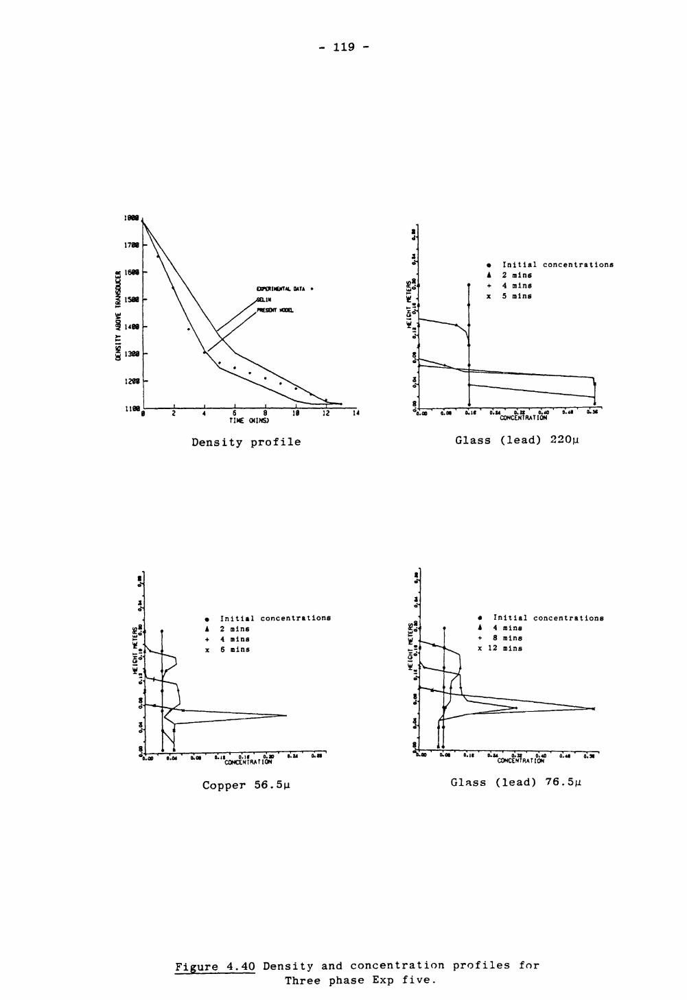
- 119 -

1808

MTA •

5-1

U00 6 aTIME WINS)

• Initial concentrationsA 2 rains+ 4 minex 5 mins

0.00 o.o* 0.14 O.B 0.40 CONCENTRATION

0.3t

Density profile Glass (lead) 220u

• Initial concentrationsA 2 mlns+ 4 mlnsx 6 inins

• Initial concentrations A 4 rains +• 8 mins x 12 mins

o oo O.M o.o» 9. II O.K 0.30 O.I*CONCENTRATION

0.1* 0.24 O.H 0.40CONCENTRATION

O.M 0.91

Copper 56.5u Glass (lead) 76.5\i

Figure 4.40 Density and concentration profiles forThree phase Exp five.

- 120 -

a* r*

g0s

4 6 TI>C WINS)

Density profile

9 Initial concentrationsA 30 sees+ 60 seesx 90 sees

Glass (lead) 362.5u

§25 .

8

• Initial concentrations A 1 ain + 2 nins x 4 mins

ti' *

o.oo O.M a.it O.U O.B 0.40 o.a e.M CONCENTRATION

Glass (lead) 220u

• Initial concentrationsA 2 nine•»• 4 Binsx 8 mins

0.11 o.it o.a CONCENTRATION

Glass (lead) 120u

Figure 4.41 Density and concentration profiles forThree phase Exp six.

UI 4"

- 121 -

1) All three phases

2) Two slower moving phases

3) Slowest moving phase only.

The predicted solids concentrations associated with each experiment for

the first two layers are:

Experiment Solid concentration in DH Solids concentration in D

Exp one

Exp two

Exp three

Exp four

Exp five

Exp six

first sediment layer

0-687

0-660

0-653

0-688

0-690

0-647

53/u

106a

93ju

49 v

48u

96u

second sediment

0-621

0-633

0-658

0-621

0-658

0-624

layerH

29u

50/u

30M

Table 4.5 Sediment concentrations associated with three phase runs.

The solids concentration in the third layer is (l-E(D^)) where E(d^)

is the voidage of the slowest moving phase when packed alone. Further

densif ication of the sediment in the layer consisting of all three

phases occurs for Exp two and Exp three only. The hydraulic radius

associated with the second layer for each experiment is smaller than the

smallest phase present, therefore no more compaction in this layer can

occur. The movement of the smallest phases into the first sediment

layer for Exp two and Exp three will continue until the solids

concentration in this layer is 0-698 and 0-677 respectively.

Although this movement will occur within the structure of the sediment

it will not occur from the free settling zone just above the sediment

until the zone containing all three phases has disappeared. This is

because the movement of the smallest particles in this zone is in the

opposite direction to the other phases.

- 122 -

CHAPTER FIVE

MODELLING A CONTINUOUS GRAVI TY

THICKENER

- 123 -

5.1 Introduction

The theoretical description of thickening is still very poorly

understood. As discussed in chapter one the majority of thickeners are

designed using data obtained from laboratory batch tests (i.e. Jar

tests) on the slurry to be dewatered. This involves noting the height

of the slurry/supernatant liquid interface over time and using material

balances with the assumption that settling velocity is dependent on

concentration only to estimate the thickener surface area required to

give a specified dewatering. It is common knowledge that these design

procedures are inadequate and large scale safety factors must be

incorporated into the thickener design, Pearce (1977). This is because

the use of laboratory batch tests inherently assumes that batch settling

is analogous to continuous industrial thickening.

Due to the non homogeneity of the feed it is essential to model an

industrial continuous thickener as a multiphase problem. Account of the

forces present in the system was considered by Dixon (1977) by

incorporating a momentum balance equation for the solids particles which

he assumed had the same properties. The following multiphase numerical

model has been developed to simulate the performance of a thickener

using the same assumptions stated for batch sedimentation, see section

4.1, except assumption (1). Also assumption (2) is an approximation

especially where the feed separates into the upflow and downflow

streams. Modelling a thickener as a multidimensional, multiphase

problem would involve solving pressures for each phase in each

direction. At the present time solution procedures cannot solve a

problem of this complexity. Therefore a one dimensional model is

assumed so that the multiphase effects can be analysed. It is also

assumed that particles do not settle at the underflow and overflow

streams.

- 124 -

5. 2 Governing Equations

The governing equations describing the thickening process are

essentially the same as for batch sedimentation, see chapter four,

except account must be taken of the following:

1) Feed

2) Underflow

3) Overflow

4) Upflow

5) Downflow.

The above streams and flow influences can be incorporated into the batch

model by making appropriate adjustments to the governing equations and

boundary conditions.

5.2.1 Solid phase equations

Associated with each solid phase is a continuity and momentum equation.

The momentum equation is the same as used for batch sedimentation, see

equation 4.2. The influence of the upflow and downflow effects on the

particles is taken into account via the fluid velocity in the drag term.

The presence of the feed is incorporated into the continuity equation

which is adjusted as follows:

= M (5.1)

where

- 125 -

M = at feed (5. la)Q ay

= 0 elsewhere (5.1b)

Tp and Sp are the volumetric flow rates and concentrations associated

with the feed. Q Ay is the volume of the control volume representing

the feed where Q is the surface area.

5.2.2 Fluid phase equations

Associated with the fluid phase is the fluid continuity equation and the

concentration balance equation. For a thickener the concentration

balance equation is the same as used in batch sedimentation, see

equation (4.9). As with the solid phases the fluid continuity equation

is adjusted to incorporate the feed streams:

if (PfF) + ~ (PfFV) = N (5.2)

T F N = pf -r^-^ at feed (5.2a)

0 elsewhere (5.2b)

^p being the volumetric fluid concentration of the feed stream.

As the solids and fluid phases are incompressible the density terms can

be eliminated from equations 5.1 and 5.2. Combining the resulting

equations gives the total volumetric balance equation for a thickener

NSOLa(FV) ^ay < S i U i> = V

- 126 -

where

V = at feed (5.3a)

0 elsewhere (5.3b)

5.2.3 Boundary Conditions

Boundary conditions must be given at the underflow and overflow outlets

(i.e. Y=l and Y=NY respectively). Due to the assumption that

particulate settling does not occur in the underflow or overflow then

the following boundary conditions will apply:

T U i (i=l...,NSOL), V = - -"- at underflow (i.e. Y=l) (5.4a)

XI

T~- at overflow (i.e. Y=NY) (5.4b)QNY

Also the concentrations at these boundarys are the same as calculated at

the underflow and overflow control volume nodal points. Therefore at

the boundaries

5.3 Control Volume representation

The thickener domain is divided into a number of control volumes, see

figure 5.1. Because of the non-uniform shape of the thickener and the

area to be modelled, see figure 3.1, control volumes of different

surface area are applied at the feed well outlet and around the conical

section at the base. The surface area of each control volume is given

- 127 -

overflow cell

Feed cell

-X-

^TvT\TT \\\\\\\U\\\\\\\\\ •. ; .-. . •, x •.;. ;.,••,,^^^xx&xxxxW,'/7//7/////7/7//////7.-7'7////

-X-

•-*-

\\\\\\\\\\\\\\\\\\\\\\\\\\\l(XX

Y/7//7/, ////'{/////////////A

underflow cell

scalar cells scalar nodes

velocity cells X velocity nodes

Figure 5.1 Control volume specification for a thickener

- 128 -

by:

Q = irR 2 (5.4)

where R is the radius of the control volume. The value of R for all

cells below the feed cell and above the cell containing the top of the

conical section is given by

(5.5,

where TDIAM is the diameter of the thickener. The value of R for

all cells above the feed cell is given by

o TDIAM - WDIAMR = —————-————— (5.6)

where WDIAM is the diameter of the feed well. This ensures that only

the area outside the feed well is modelled. For control volumes within

the conical section (not applicable for flat bed thickeners) down to and

including the underflow cell, see figure (5.2c), the value of R is

given by

TDIAMTAN(0)

The control volumes containing the feed outlet and the top of the

conical section, see figures (5.2a) and (5.2b), involve calculating the

volume of the thickener at these locations which is to be modelled.

This volume will correspond to the volume of the cells representing

these locations. For the feed cell this volume is:

- 129 -

TDIAM

, WDIAM >

tAy+ Ay

Figure 5.2a Control volumes around the feed well

Ay-r i-Ay+

Ay

Figure 5.2b Control volumes at top of conical section

Figure 5.2c Control volumes within the conical section

- 130 -

VOL = (TDIAM) 2 Ay - (WDIAM) 2 &y+ (5.8)

This again ensures only the volume outside the feed well is under

consideration. The volume of the cell containing the top of the conical

section is:

VOL = TDIAM - AY+ + (TDIAM) 2 AV_ (5.9)

The surface area of these two control volumes is calculated via:

(5.10,

5.4 Discretised equations

The governing equations are discretised using the techniques outlined in

chapter four, see section 4.3, to give discretised equations of the form

(4.12).

Consider the control volumes in figure 5.3. It can clearly be seen that

the difference in the surface .area of some control volumes will effect

the inflow and outflow contributions. To incorporate this effect the

following variables are calculated:

(S.lla)

A 2 = (5.lib) QR

- 131 -

Qt

N

Qt

Qc

Qi

• N Qp-

• P

Figure 5.3 Surface Areas associated with control volumes

Now if

- 132 -

A t > 1 then = 1 (5. lie)

A 2 ^ 1 then A 2 = 1 (5. lid)

Therefore A t and A 2 represent the proportions of the dependent

variable that can flow across the north and south faces of the

control volume respectively.

Because of the source terms associated with the continuity equations at

the feed as well as the different surface areas of the control volumes

the discretised equations will contain different coefficients for all

the governing equations except the concentration balance which remains

the same, see equation (4.16).

5.4.1 Solid phase continuity

The continuity equation (5.1) is integrated over the scalar control

volumes. This results in equation (4.12) where <& is the solid

concentration S and:

AN = tt-UD , OB A t (5.12a)

AS _ IUC , OB A (5.12b)

AP = At * (5.12c)

b = SOLD * X p (5.12d)

- 133 -

where

for feed cell (5.12e) Qp

= 0 elsewhere (5.12f)

5.4.2 Solid phase momentum

The momentum equation of each solid phase is integrated over velocity

control volumes. The coefficients associated with equation (4.12),

where o is the solid velocity U, are the same as for batch

sedimentation see section 4.3.2. The only difference is due to the

different surface areas associated with some control volumes.

Considering the inflow contributions these become:

AN = AN* A t (5.13a)

AS = AS* A 2 (5.13b)

where AN and AS are the values given in section 4.3.2. The new

values of AN and AS given by equations (5.13a) and (5.13b) are used

to calculate AP in the usual manner.

5.4.3 Total volumetric balance

Equation (5.3) is integrated over scalar control volumes to give a

discretised equation of the form (4.12) where <D is the fluid velocity

v. The coefficients associated with equation (4.12) are given by

equations (4.18) except the source term b which is given by:

- 134 -

NSOLI

{*-<SI) N FLOW (5.14)

where

uFLOW = - — if cell is below feed cell (5.14a)

— for feed cell and above (5.14b)

The terms given by equations (5.14a) and (5.14b) represent the downflow

and upflow velocity effect, where Qp is the surface area of the

appropriate control volume.

5.5 Solution procedure

In modelling a continuous gravity thickener the following information is

required:

1) Volmetric flow rates of the feed (Tp) and the underflow (Ty) .

The overflow volumetric flow rate is then calculated via:

TO = TF - TU (5.15)

2) Dimensions of the thickener which include:

Diameter of thickener.

Depth of thickener from slurry surface to the underflow outlet

Conical angle associated with a conical base thickener.

Distance from underflow outlet at which conical section begins

Depth of feed well from slurry surface to feed well outlet.

Diameter of feed well.

- 135 -

3) Volumetric concentrations of each solids phase present in the feed

(SF ).

Given the above information the model predicts:

1) Clarity of overflow.

2) Solid concentration in underflow.

3) Distribution of solids throughout the thickener.

If weight concentrations (C^) and mass flow rates (W) are given

instead of volumetric concentrations (S^) and flow rates (T) then

volumetric values are calculated via:

= — Cj (5.16) Pi

T = — (5.17)

where the pulp density (p) is given by equation (4.8) or

Pf p = —————————— £ ————————— (5 . 18)NSOL _ NSOLK I -l ci=l 1=1

Using the dimensions of the thickener a one-dimension control volume

representation is set up, see figure 5.1. Unlike batch sedimentation

the operation of a continuous gravity thickener is a steady state

process. The model assumes initially that the thickener is full of

water only. The effect of the feed and underflow streams are modelled

by solving the dependent variables S-^, U^ (i = l. . . ,NSOL) , F and V

- 136 -

throughout the thickener over time until a steady state solution has

been obtained. The upflow and downflow effects are directly

incorporated into the "total volumetric balance" equation which is

solved for the fluid velocity. These flow effects will be felt by the

solid particles via the. drag term in the momentum equations which have

the fluid velocity incorporated within them.

The discretised equations are solved using the same procedure as for

batch sedimentation, see section 4.5, with the following adjustments:

• Due to the overall slurry movement, the boundaries associated with

each phase and the sediment are not monitored, Although the packing

model is still used to check what cells become packed.

If a cell becomes packed then the velocities associated with that

cell are set to the upflow or downflow velocity at that cell

depending on the location of the cell

T Ui (i=l,NSOL), V = - -^ if cell is below feed cell. (5.19)

T—if cell is feed cell or above. (5.20)

The solution procedure stops when a steady state solution has been

obtained. If the total solids mass in the thickener as well as the

dependent variables do not change significantly between two time

steps then steady state has been achieved. The mass of solids in a

control volume is given by

- 137 -

NSOL TMASS = ^ Si Pi Q Ay (5.21)

combining the mass present in each control volume will give the

total solids mass in the thickener.

5.6 Comparison with experimental data

The data gathered at the mineral processing plant, see chapter three,

has been used in validating the above model. The fluid phase in each

thickener is water and the density and viscosity values used are those

at room temperature. Therefore

pf = 1000 Kg/M 3

ju f = 0-001 Kg/MS.

For each of the three thickeners the underflow and overflow scalar nodes

are situated 3cm from the thickener base and slurry surface

respectively. The thickener domain is divided into nineteen control

volumes with the cells between the underflow and overflow cells being of

uniform size. All information needed to simulate each thickener is

available except the depth of the feed well which is assumed to be

approximately a third of the thickener height. The voidages E(di)

associated with the packing model are taken as 0-4 for each of the

materials under investigation. The experimental data consists of mass

flow rates and concentration profiles by weight. The model uses

equations (5.15), (5.16) and (5.17) to convert the input data into

volumetric terms and outputs concentrations as weight fractions.

- 138 -

5.6.1 Galena Thickener

The Galena thickener is a flat bed thickener containing Galena and small

quantities of Barytes and Fluorite. The volumetric flow rates of the

feed, underflow and overflow are calculated from the mass concentrations

of each material present in these streams as well as their mass flow

rates. Therefore:

TF = 0-003364 M 3 /S

= 0-002016 M 3 /S

TO = 0-001348 M 3 /S.

The domain of the thickener, see figure 3.11, is divided into control volumes whose surface areas are:

distance of scalar

node from underflow (M)

1-64

1-56

1-47

1-38

1-29

1-20

1-11

1-02

0-92

0-83

0-74

0-65

0-56

0-47

0-37

0-28

0-19

0-10 0-03

surface area

of control volume (M z )

38-8

38-8

38-8

38-8 38-8

38-94

39-59

39-59

39-59

39-59

39-59

39-59

39-59

39-59

39-59

39-59

39-59

39-59

39-59

Table 5.1 Surface areas associated with Galena thickener

- 139 -

The depth of the feed well below the slurry surface was taken to be

0-5m. The size distribution of the Galena, Barytes and Fluorite present

in the feed are assumed to be the same and are given in figure 3.12. By

using the average particle diameter and the presence of the three

materials we are modelling a three phase problem, see table 5.2a. The

size distribution is split into two and three equal parts giving a six

and nine phase (A) problem where the concentrations of the phases

belonging to any one of the materials are equal, see tables (5.2b) and

(5.2c). The diameters of each phase correspond to the central location

of each split section from the size distribution. Therefore the

diameters in the six phase model corresponds to the 75% and 25%

undersize points in figure 3.12. Comparing the model using three, six

and nine phase (A) data against experimental data, see figure 5.4, it

can be seen that representing the feed distribution in greater detail

enables closer comparisons with the experimental solids concentration

profile throughout the thickener to be made. The underflow concen­

tration is predicted in all cases but for each run no solids are present

in the overflow. To incorporate smaller particles into the model the

size distribution was split into three parts consisting of the smallest

5% with the other 95% being split into two equal parts, see table

(5.2d). Nine phase (B) predicts the overall solids profile with a

greater degree of accuracy than the other comparisons. Solids are also

present in the overflow, see table (5.4a) and (5.4b), which consists of

Barytes and Fluorite only, although chemical analysis of the overflow

predicted a quantity of Galena as well as Barytes and Fluorite being

present. The quantities of each material present in the underflow

compares favourably with the values given by chemical analysis. The

reason no Galena is present in the overflow is probably due to:

Phase

Conc

entr

atio

n (WT*)

Diameter (M)

Density

(Kg/M

3 )

Phas

eConcentration

(WT%)

Diam

eter

(M)

Density

(Kg/M

3 )

Phase

1Co

ncen

trat

ion

(WT*)

53-23

Phas

eConcentration

Diameter (n)

Dens

ity

(Kg/M

3

1)

17-743

817500 1

%)

25-284

717500

Diameter

Density

Table

5.

(WT*)

>

Tabl

e 5.

217-743

387500

Table

5.

225-284

237500

(At)

38(Kg/M

3 )

7500

2a Three

phase

data for

1 2

26-615

26-615

69

217500

7500

2b

Six

phase

data for

3 4

17-743

-97

15

81

2 3

2-91

4-88

38

384500

3100

Gale

na Thickener

345

1-455

1-455

2-44

69

21

694500

4500

3100

Galena Thickener

567

97

-97

1-627

38

15

817500

4500

4500

4500

3100

2c

Nine phase

(A)

data

3 4

2-66

2 1-

382

4 71

7500

4500

for

Galena Th

icke

ner

567

1-382

-146

2-

318

23

4 71

4500

4500

3100

6 2-44 21 3100

8 9

1-62

7 1-

627

38

1531

00

3100

8 9

2-318

-244

23

43100

3100

Table

5.2d

Nine

phase

(B)

data for

Galena Th

icke

ner

- 141 -

LU_J H- ZD

O

LUa

o00

o •—«LU

EXPERIMENTAL DATA *•THREE PHASES•SIX PHASES

•NINE PHASES (A)•NINE PHASES (B)

0. 3 0. 4 0. 5CONCENTRATION (WEIGHT)

Figure 5.4 Comparisons between model and experimental data for Galena thickener

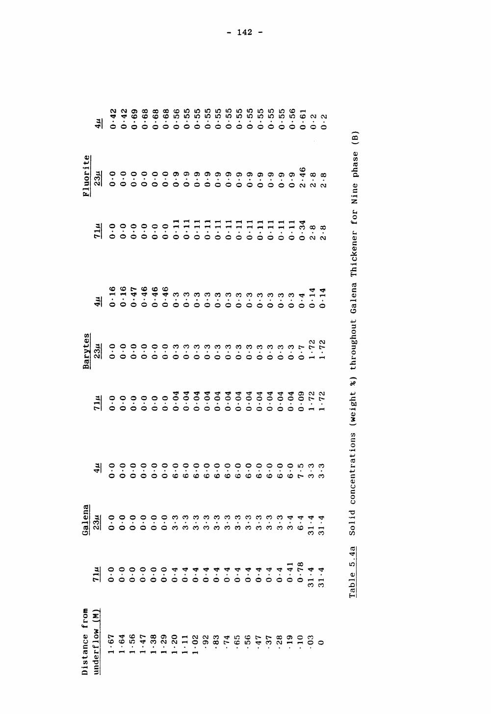
Distance fr

omunderflow

(M)

1-67

1-64

1-56

1-47

1-38

1-29

1-20

1-11

1-02 •92

•83

•74

•65

•56

•47

•37

•28

• 19

•10

•03

0

1 71*i

0-0

0-0

0-0

0-0

0-0

0-0

0-4

0-4

0-4

0-4

0-4

0-4

0-4

0-4

0-4

0-4

0-4

0-41

0-78

31-4

31 -4

Galena

23n

0-0

0-0

0-0

0-0

0-0

0-0

3-3

3-3

3-3

3-3

3-3

3-3

3-3

3-3

3-3

3-3

3-3

3-4

6-4

31-4

31-4

4*i

0-0

0-0

0-0

0-0

0-0

0-0

6-0

6-0

6-0

6-0

6-0

6-0

6-0

6-0

6-0

6-0

6-0

6-0

7-5

3-3

3-3

71*i

0-0

0-0

0-0

0-0

0-0

0-0

0-04

0-04

0-04

0-04

0-04

0-04

0-04

0-04

0-04

0-04

0-04

0-04

0-09

1-72

1-72

Barytes

23*i

0-0

0-0

0-0

0-0

0-0

0-0

0-3

0-3

0-3

0-3

0-3

0-3

0-3

0-3

0-3

0-3

0-3

0-3

0-7

1-72

1-72

4M 0-16

0-16

0-47

0-46

0-46

0-46

0-3

0-3

0-3

0-3

0-3

0-3

0-3

0-3

0-3

0-3

0-3

0-3

0-4

0-14

0-14

71*i

0-0

0-0

0-0

0-0

0-0

0-0

0-11

0-11

0-11

0-11

0-11

0-11

0-11

0-11

0-11

0-11

0-11

0-11

0-34

2-8

2-8

Fluorite

23*i

0-0

0-0

0-0

0-0

0-0

0-0

0-9

0-9

0-9

0-9

0-9

0-9

0-9

0-9

0-9

0-9

0-9

0-9

2-46

2-8

2-8

4*i

0-42

0-42

0-69

0-68

0-68

0-68

0-56

0-55

0-55

0-55

0-55

0-55

0-55

0-55

0-55

0-55

0-55

0-56

0-61

0-2

0-2

to I

Table

5.4a

Solid

concentrations (weight

%) throughout Galena Thickener

for

Nine phase

(B)

Dis

tanc

e fr

omun

derf

low

(M

) 71

^1-

671-

611

-52

1-43

1-34

1-25

1-15

1-06

0-97

0-88

0-79

0-70

0-61

0-52

0-43

0-33

0-24

0-15

0-06 0

•347

-04

-•117-0

1-•

11

7-0

1-•

11

7-0

1-•

117-0

1-•

10

7-0

1-•

102-0

1-•

102-0

1-•

102-0

1-•

102-0

1-•

102-0

1-•

102-0

1-•

102-0

1-•

102-0

1-•

10

2-0

1-•

10

2-0

1-•

10

2-0

1-•

972-0

2-•

48

1-0

2-•

50

9-0

4

Gal

ena

23/u

•347

-04

-•136-0

2-•

134

-02

-•134

-02

-•134

-02

-•122-0

2-•

12

2-0

2-•

122-0

2-•

12

2-0

2-•

12

2-0

2-•

12

2-0

2-•

122-0

2-•

122-0

2-•

12

2-0

2-•

12

2-0

2-•

12

2-0

2-•

122-0

2-•

116-0

2-•

58

2-0

3-•

50

9-0

4

4M•3

47-0

4-•

79

7-0

5-•

731-0

5-•

73

3-0

5-•

73

3-0

5-•

30

2-0

5-•

71

2-0

4-•

71

5-0

4-•

71

5-0

4-•

71

5-0

4-•

715-0

4-•

715-0

4-•

715-0

4-•

71

5-0

4-•

71

5-0

4-•

71

5-0

4-•

71

5-0

4-•

69

8-0

4-•

52

6-0

4-•

50

9-0

4

71n

•347

-04

-•662-0

2-•

652-0

2-•

65

2-0

2-•

652-0

2-•

59

3-0

2-•

565-0

2-•

565-0

2-•

56

5-0

2-•

565-0

2-•

56

5-0

2-•

565-0

2-•

56

5-0

2-•

565-0

2-•

56

5-0

2-•

565-0

2-

• 565

-02

-•536-0

2-•

22

7-0

2-•

509

-04

Bar

ytes

23ji

•347

-04

-•7

19

-03

-•708

-03

-•708

-03

-•708

-03

-•6

37

-03

-•6

65

-03

-•6

66

-03

-•6

66

-03

-•6

66

-03

-•6

66

-03

-•6

66

-03

-•6

66

-03

-•6

66

-03

-•6

66

-03

-•6

66

-03

-•6

66

-03

-•6

33

-03

-•2

81

-03

-•5

09

-04

4/J

•347

-04

•118

-04

•121

-04

•121

-04

•121

-04

•148

-04

-•54

3-0

4-•

54

6-0

4-•

54

6-0

4-•

54

6-0

4-•

54

6-0

4-•

54

6-0

4-•

54

6-0

4-•

54

6-0

4-•

54

6-0

4-•

54

6-0

4-•

54

6-0

4-•

535-0

4-•

434

-04

-•5

09

-04

71/u

•347

-04

-•4

05-0

2-•

39

9-0

2-•

39

9-0

2-•

39

9-0

2-•

359

-02

-•34

1-0

2-•

34

2-0

2-•

34

2-0

2-•

34

2-0

2-•

34

2-0

2-•

34

2-0

2-•

34

2-0

2-•

34

2-0

2-•

34

2-0

2-•

34

2-0

2-•

34

2-0

2-•

32

1-0

2-•

101-0

2-•

50

9-0

4

Flu

ori

te23

/i•3

47-0

4-•

418

-03

-•4

11-0

3-•

41

1-0

3-•

411-0

3-•

36

5-0

3-•

40

6-0

3-•

40

7-0

3-•

40

7-0

3-•

407-0

3-•

40

7-0

3-•

407-0

3-•

40

7-0

3-•

407-0

3-•

407-0

3-•

407-0

3-•

40

7-0

3-•

38

5-0

3-•

14

0-0

3-•

509

-04

4M•3

47-0

4•2

10-0

4•2

12-0

4•2

12-0

4•2

12-0

4•2

32-0

4-•

464

-04

-•4

66

-04

-•4

66

-04

-•4

66-0

4-•

46

6-0

4-•

46

6-0

4-•

46

6-0

4-•

466-0

4-•

466-0

4-•

466-0

4-•

466-0

4-•

460-0

4-•

39

1-0

4-•

509

-04

CO I

Table

5.4b

Solid

velocities throughout Galena Thickener

for

Nine phase

(B)

- 144 -

Greater breakdown of size distribution needed to incorporate even

smaller particles into the model.

One dimensional assumption.

Errors in experimental data

Flocculation, where Galena has agglomerated with other material

lowering the overall density.

Also the poor comparison with experimental data above the feed well

outlet is due to the assumed feed well depth.

The total mass of solids at steady state and the time it takes to reach

steady state as well as the computing time for each run is:

Run

Three phase

Six phase

Nine phase (A)

Nine phase (B)

Solids mass in Thickener

6932 Kg

8393 Kg

9725 Kg

11710 Kg

Time to reach steady state

3 hours 30 mins

4 hours

5 hours

12 hours

CPU time

67 sees

23 mins

32 mins

50 mins

Table 5.3 Steady state details and computing time for Galena thickener

5.6.2 Fluorite Thickener

The fluorite thickener is a conical base thickener containing fluorite

only. The volumetric flow rates of the feed, underflow and overflow

are:TF = 0-01246 M 3 /S

TU = 0-0055 M 3 / s

T0 = 0-00696 M 3 /S

- 145 -

The thickener domain, see figure 3.6, is divided up into control volumes

whose surface areas are:

distance of scalar

node from underflow (M)

2-94

2-83

2-66

2-49

2-32

2-16

1-99

1-82

1-65

1-49

1-32

1-15

0-98

0-81

0-65

0-48

0-31

0-14 0-03

surface area

of control volume (M 2 )

174

174

174

174

174

174-2

174-8

174-8

174-8

174-8

174-8

174-8

174-8

165-6

113-266-3

31-8

9-9

2-1

Table 5.5 Surface areas associated with Fluorite thickener.

The depth of the feed well below the slurry surface is taken to be

0-87m. The fluorite size distribution for the feed is split equally

into two, five and ten parts and particle diameters for each phase are

estimated, see tables (5.6a), (5.6b), (5.6c) and (5.6d). Comparing the

model predictions at steady state with the obtained experimental data,

see figure (5.5), it can be seen that although the underflow is

predicted in all cases the greater break down of the feed does not

predict the experimental data. The fact that the one and two phase runs

give better predictions is probably because flocculation is playing a

major role in this thickener creating bigger particles (i.e. floes)

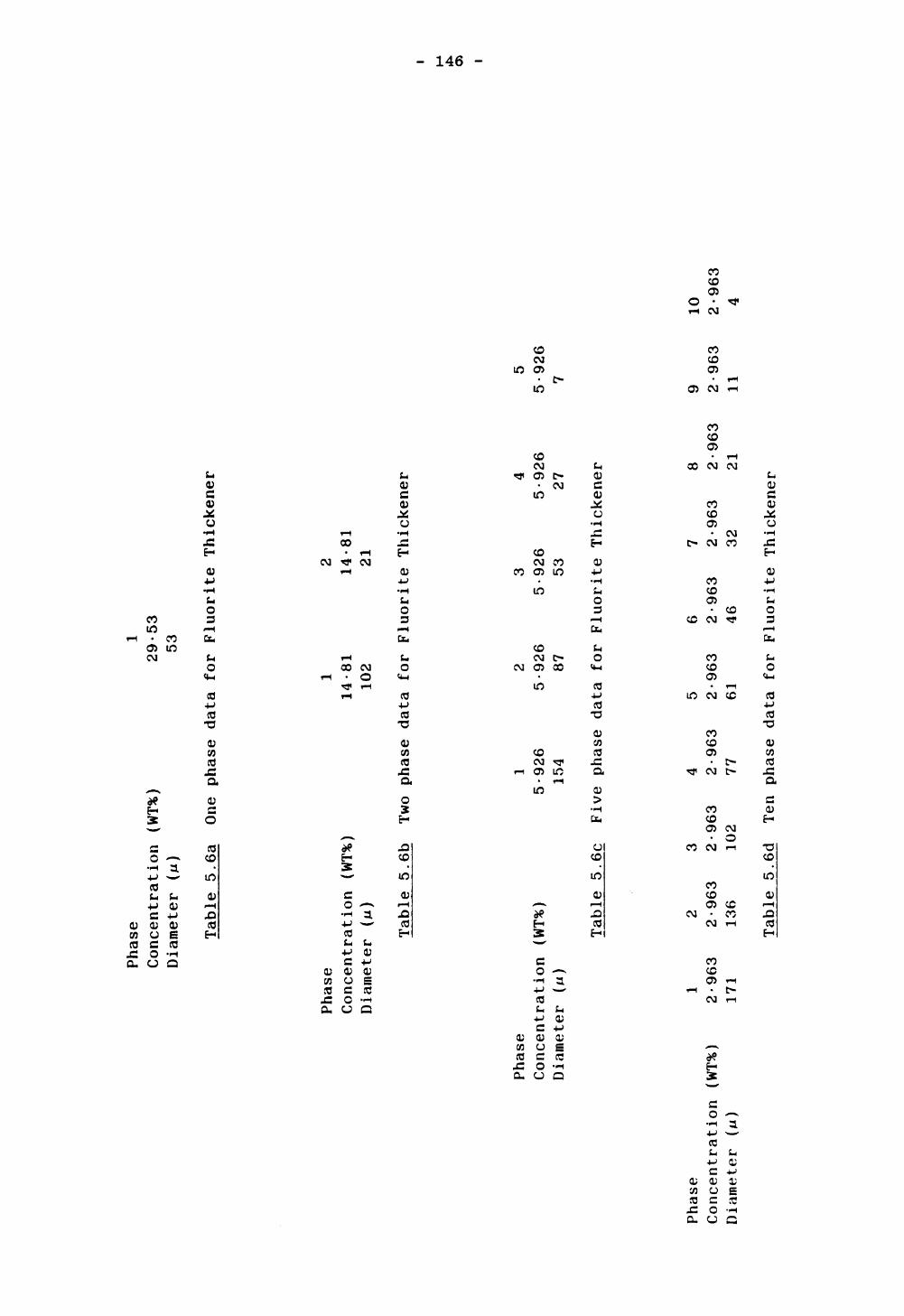
Phase

1Co

ncen

trat

ion

(WT%

) 29-53

Diam

eter

(M)

53

Table

5.6a

One

phase

data fo

r Fl

uori

te Th

icke

ner

Phas

e 1

2Conc

entr

atio

n (WT%)

14-81

14-81

Diameter (n)

102

21

Table

5.6b

Two

phase

data fo

r Fl

uori

te Th

icke

ner

Pha

se

12

34

5C

once

ntr

atio

n

(WT%

) 5-

926

5-92

6 5-

926

5-92

6 5-

926

Dia

met

er

(n)

154

87

53

27

7

Tabl

e 5.6c

Five phase

data

fo

r Fluorite Th

icke

ner

o> i

Pha

se

1234

5678

9

10C

once

ntr

atio

n

(WT%

) 2-

963

2-96

3 2-

963

2-96

3 2-

963

2-96

3 2-

963

2-96

3 2-

963

2-96

3D

iam

eter

(M

) 17

1 13

6 10

2 77

61

46

32

21

11

4

Table

5.6d

Ten

phas

e data fo

r Fl

uori

te Th

icke

ner

- 147 -

LU

EXPERIMENTAL DATA *

•ONE PHASE

•TVO PHASES

•FIVE PHASES

,TEN PHASES

0. 2 0. 3 0. 4CONCENTRATION (WEIGHT)

Figure 5.5 Comparisons between model and experimental data for Fluorite thickener

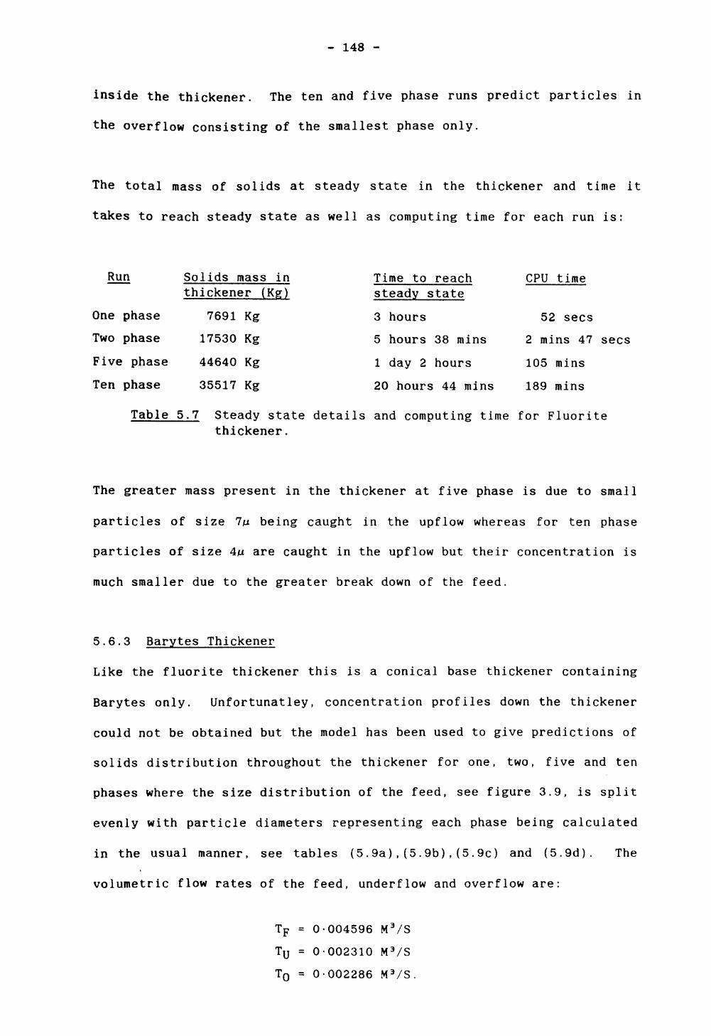
- 148 -

inside the thickener. The ten and five phase runs predict particles in

the overflow consisting of the smallest phase only.

The total mass of solids at steady state in the thickener and time it

takes to reach steady state as well as computing time for each run is:

Run

One phase

Two phase

Five phase

Ten phase

Solids mass in thickener (Kg)

7691 Kg

17530 Kg

44640 Kg

35517 Kg

Time to reach steady state

3 hours

5 hours 38 mins

1 day 2 hours

20 hours 44 mins

CPU time

52 sees

2 mins 47 sees

105 mins

189 mins

Table 5.7 Steady state details and computing time for Fluorite thickener.

The greater mass present in the thickener at five phase is due to small

particles of size 7n being caught in the upflow whereas for ten phase

particles of size 4n are caught in the upflow but their concentration is

much smaller due to the greater break down of the feed.

5.6.3 Barytes Thickener

Like the fluorite thickener this is a conical base thickener containing

Barytes only. Unfortunatley, concentration profiles down the thickener

could not be obtained but the model has been used to give predictions of

solids distribution throughout the thickener for one, two, five and ten

phases where the size distribution of the feed, see figure 3.9, is split

evenly with particle diameters representing each phase being calculated

in the usual manner, see tables (5.9a),(5.9b),(5.9c) and (5.9d). The

volumetric flow rates of the feed, underflow and overflow are:

TF = 0-004596 M 3 /S

TU = 0-002310 M 3 /S

TO = 0-002286 M 3 /S.

Phase

Concentration

(WT%

) Di

amet

er (M)

33-119

28-5

Table

5.9a

One

phase

data fo

r Ba

ryte

s Th

icke

ner

Phase

Conc

entr

atio

n (W

T%)

Diam

eter

(M)

16-5

595

4816

-559

5 16

Table

5.9b

Tw

o phase

data for

Barytes

Thic

kene

r

Phase

Concentration

(WT%)

Diameter (M)

16-6238

74

26-6238

42

36-6238

28-5

46-6238

18

56-6238

9

Table

5.9c

Five phase

data for

Barytes

Thickener

(0 I

Pha

se

1 234

5678

9

10C

once

ntr

atio

n

(WT%

) 3-

312

3-31

2 3-

312

3-31

2 3-

312

3-31

2 3-

312

3-31

2 3-

312

3-31

2D

iam

eter

(M

) 85

63

48

37

-5

32

26

21

16

12

6

Table

5.9d

Ten

phase

data fo

r Bary

tes

Thickener

- 150 -

The thickener domain, see figure 3.8, is divided into a number of

control volumes whose surface areas are:

Distance of scalar

node from underflow (M)

3-89

3-75

3-53

3-30

3-08

2-86

2-63

2-41

2-19

1-96

1-74

1-51

1-29 1-07

•84

•62

•39

•17

•03

Surface area

of control volume (M*)

44-82

44-82

44-82

44-82

44-93

45-60

45-60

45-60

45-60

45-60

45-60

45-60

45-60

45-60

45-60

45-60

40-49

11-88 1-78

Table 5.8 Surface areas associated with Barytes thickener

The depth of the feed well below the slurry surface was assumed to be

0-92m. Comparisons between the model and experimental data, see figure

5.6, show that increasing from five to ten phases does not make a

significant difference in the solids profile although for ten phases the

6.2^ phase does incorporate itself in the upflow stream but over­

estimates the amount of solids present in the overflow. The solids

concentration in the underflow is predicted accurately by each run.

- 151 -

UJ

EXPERIMENTAL DATA *

•ONE PHASE

TVO PHASES

0. 2 0. 3 0. 4CONCENTRATION (WEIGHT)

Figure 5.6 Comparisons between model and experimental data for Barytes thickener

- 152 -

The total mass of solids at steady state and time it takes to reach

steady state as well as the computing time for each run are:

Run

One phase

Two phase

Five phase

Ten phase

Solids mass in thickener (Kg)

8867 Kg

13021 Kg

16960 Kg

18282 Kg

Time to reach steady state

4 hours 11 mins

7 hours 6 mins

12 hours 24 mins

Iday 1 hour

CPU time

2 mins 4 sees

9 mins 34 sees

46 mins 17 sees

224 mins

Table 5.10 Steady state details and computing time for Barytes thickener

- 153 -

CHAPTER SIX

A NUMERICAL MODEL FOR FLOCCULATED

BATCH SEDIMENTATION

- 154 -

6.1 Introduction

The major method of increasing the efficiency of solid/liquid

separations is through the use of aggregating or agglomerating chemical

additives known as flocculants or coagulants. Both these additives

produce small clusters of particles (plus enclosed fluid) called floes.

Coagulants are used to break down the repulsive forces around the

particles enabling the attractive London-van de Waals forces to

dominate. Flocculants form bridges bonding the particultes together,

see Wills (1985). Particulate mixtures in which either of the above

effects are occurring will be referred to as flocculated mixtures.

Like non-flocculated mixtures two regions will form during the

settlement of particulates in a flocculated mixture, see figure 6.1,

these are:

1) Free settling region

2) Sediment region.

The free settling region will consist of discrete particles settling at

different velocities due to their differences in density and/or size and

shape. These particulates will collide and form floes which can grow in

size, due to further collision, until a maximum stable size is reached.

The weight of the particulates and floes in the free settling region is

borne solely by hydraulic forces. As the floes and particulates settle

they will pack from the base up and form the sediment region. The

solids concentration at which this occurs is known as the compression

point and depends on the structure and concentrations of the floes and

particulates present. Within the sediment the floes lose their

individual identity but the attractive/bonding forces between the

particles form a particulate structure which can be broken down when the

weight of particulates above becomes too great for these forces to

support. This leads to a sediment which is compressible.

- 155 -

free settling region

t compressedsediment

I

Figure 6.1 Region associated with flocculated suspensions

- 156 -

The following multiphase numerical model has been developed to simulate

the settling process associated with flocculated particulate mixtures.

This model is an extension of the non flocculated model with the same

assumptions, see Chapter four. One extra assumption is made that the

density of the solids making up the floes is constant.

6.2 Floe build up in free settling region

The build up and movement of floes in the free settling region can be

monitored by assigning a continuity and momentum equation to each floe

phase. The free settling region will initially contain only primary

particles and these will form floes due to collisions and the

attractive/bonding forces present, see figure 6.2.

<s o o o o o o o

O

&Floes Primary Particles

Figure 6.2 Solids present in free settling region.

Like each primary particulate phase the floe phases will be distinct via

their size, density and shape. The density of a floe must take into

account the enclosed fluid which is assumed to be stationary as well as

the solids present in the floe. The build up of floes can be incorpor-

- 157 -

ated into the model by making appropriate adjustments to the continuity

equations. These adjustments are based on the following population

balances.

6.2.1 Smoluchowski population balances

The flocculation of particles in a liquid depends upon the collisions

between particles, caused by their relative motion. Smoluchowski (1917)

developed population balances which have been used to model such

phenomena. The relative motion can be due to Brownian movement or by

external forces acting on the particles such as gravity. Two types of

floccu- lation can occur, these are:

1) Perikinetic flocculation

2) Orthokinetic flocculation.

Perikinetic flocculation is due to the Brownian movement causing

collisions. This form of flocculation becomes important for particles

in the sub-micron range only, see Moir (1980). Orthokinetic floccu­

lation is due to velocity gradient, caused by external forces. The

following analysis is only concerned with Orthokinetic flocculation due

to gravity. Smoluchowski assumed that all particles and floes are

spheres and that all collisions resulted in the formation of floes (i.e.

rapid flocculation). Consider figure (6.3) where particles i and j

are undergoing sedimentation. Ignoring the viscous effects encountered

when particles move closer together, particles i and j will collide

if the distance between their paths of motion x satisfies

x ^ * dij (6.1)

where

d ij = d i + dj (6.2)

- 158 -

X

END VIEW

SIDE VIEW

Figure 6.3 Smoluchowski Model

- 159 -

Consider the cylinder of diameter djj centered on particle i, the

volumetric flow rate through this cylinder is given by

= 2 rf?, n (6-3)

where u is the relative velocity. If N is the number of particles

per unit volume then the rate of collisions of j particles with the

i-particle is

dz dt |U J ~ (6.4)

The total collision rate between phases i and j per unit volume is

given by:

dz = N iNj ~ dfj | Uj - Ui | (6.5)

Smoluchowski assumed that when two particles collide they coalesce to

form a spherical particle with volume equal to that of the colliding

particles. Therefore if collisions between phases i and j result in

phase k then equa'tion (6.5) can be rewritten as:

dN, w_ 4 (6.6)

Equation (6.6) represent the rate of appearance of particles in phase

k, due to collisions between phases and j. The total rate of

change for phase k due to appearance and disappearance, where phase k

particles collide with any other particles, is given by:

- 160 -

00

dNu r» rK _ \ M M «. . _ Nk \ NlJ3i k=l. . .«. (6.7)dti+j=k 1=1

where j5 is the rate constant given by:

ifT (d^-t-dj) 2 Juj - U| J (6.8)

Equation (6.7) represents the basic Smoluchowski population balance for

coalescence of particulates.

6.2.2 Incorporating floe build up via continuity and momentum equations

Assuming floe breakdown does not occur then the above Smoluchowski

equations can be incorporated into the continuity equations as source

terms to represent the mass transfer from primary particle phases to and

between floe phases. During the sedimentation process primary particles

cannot be created as it is assumed that floe breakage does not occur.

Therefore only a disappearance term is present in the continuity

equations of primary particle phases. Appearance and disappearance

terms are present in the continuity equations for floe phases except the

largest phase (i = l) which contains only an appearance term. The

transfer of particles from one phase to another is modelled on a

volumetric basis where:

6 S,-< 6 - 9 >

substituting equation (6.9) into equation (6.7) and adding the resulting

equation to the continuity equation as a source term gives:

- 161 -

k+2 k+1S<S

ay 2 xi=NF j=i-:

c lijpk

2s,

23 „ T S i

i=NSOL

where

(6.11)

NF is the number of floe phases present given by:

NF = NSOL - NP (6.12)

where NP is the number of primary particle phases and NSOL the total

number of solids phases. The 7^j terms represent the probability that

if phases i and j collide they will form a floe. For rapid

f locculation:

rij = 1 (6.13)

7jj is dependent on the floe size and the nature of the flocculant/

coagulant being used. Ci f j >k represents the fraction of a phase k

floe formed between a collision of phase i and j particles (floes).

This is given by:

(<D 1 d i ) 3 (l-EF (di )) +(okdk )*(l-EF (dk ))

- 162 -

where Ep(dj[) is the voidage associated with a floe. Obviously for

primary particles Ep (d^) is zero as these are discrete particles with

no voidage associated with their structure. c j i k also predicts what

collisions result in a given floe size via:

ci,j,k = equation (6.14) if \C± j >T - 1|

is minimum for T = k where T=j-l...,l

= 0 if ICi - 1| is minimum for T * k. (6.15)

Notice the fraction Ci f j >k is present only in the appearance term, as

in the disappearance term a collision between a phase k particle

(floe) and any other particle (floe) will result in the loss of that

particle (floe).

Equation (6.10) is discretised in the usual manner, see Chapter four.

The only differences are due to the added source terms, this gives

different values for AP and b. The source term is linearised, see

Patankar (1980), as follows:

T'i-* (6 ' 16a)i=NSOL

k+2 k+1sc = («kdk )

i=NF j=i-

•a 3

The discretised terms for the continuity equations is given by equations

(4.13) with the following adjustment to AP and b

AP = AP* - SPAy (6.16c)

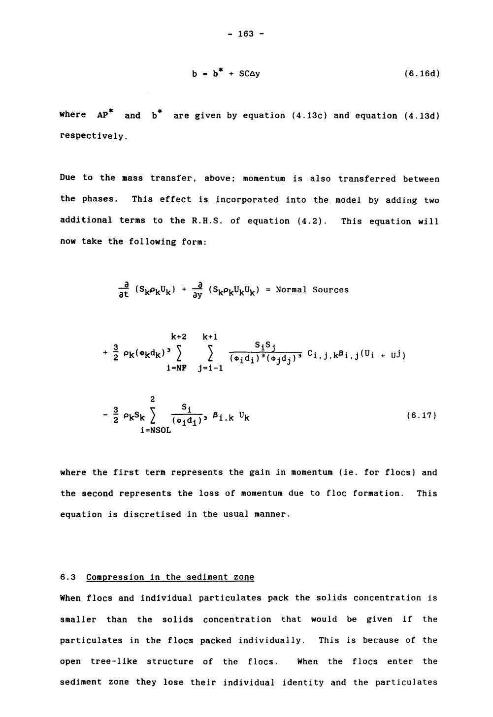
- 163 -

b = b* + SCAy (6.16d)

where AP and b are given by equation (4.13c) and equation (4.13d)

respectively.

Due to the mass transfer, above; momentum is also transferred between

the phases. This effect is incorporated into the model by adding two

additional terms to the R.H.S. of equation (4.2). This equation will

now take the following form:

+ ( skpkukuk) = Normal Sources

k+2 k-H 33 ^" T S jS .;2 Ok<*kdk) 3 } 2 (•1 d1 )»(ij dj )> c i,J,k*i.J< u i

i=NF

, (6.17)

i=NSOL

where the first term represents the gain in momentum (ie. for floes) and

the second represents the loss of momentum due to floe formation. This

equation is discretised in the usual manner.

6.3 Compression in the sediment zone

When floes and individual particulates pack the solids concentration is

smaller than the solids concentration that would be given if the

particulates in the floes packed individually. This is because of the

open tree-like structure of the floes. When the floes enter the

sediment zone they lose their individual identity and the particulates

- 164 -

in the floes settle further due to floe collapse. This process of floe

collapse gives the appearance of a consolidating sediment. The build up

and movement of the sediment zone is incorporated into the batch

sedimentation model, see Chapter four, by making appropriate adjustments

to the momentum equations and using the packing theory.

6.3.1 Incorporating compression via the momentum equations

The momentum equation for primary particles in the sediment zone is

essentially the same as equation (4.2) except for the following;

1) The fluid particle interaction terms FD is given by equation

(4.3b).

2) In the free settling region particulates and floes are in suspension

and therefore contribute to the buoyancy force exerted on the

solids. This is incorporated into the gravity term via a mixture

density (pm ). When the particulates are fully settled the

particulates do not contribute to the liquid pressure gradient and

therefore the buoyancy in the gravity term is due to the fluid alone

where pf is used instead of pm . It is assumed in this study that

throughout the sediment region the buoyancy force exerted on the

solids is dependent on the mixture density (Pm ), although this is

debatable, see Holdich (1983).

3) In the sediment region the inter-particle forces oppose the motion

of the particulates. This is incorporated into the momentum

equations by adding the following to the R.H.S. of equation (4.2).

3PS—— (6.18a)

- 165 -

where Ps is the internal pressure in the solid network. This is

assumed to be directly related to the solids concentration, see

Concha (1987); where

Ps = Ae- for F < PC(6.18b)

- 0 for F ^ Fr

and Fc is the voidage associated with the compression point. A

and B are constants that depend on the slurry being thickened and

are estimated from consolidation tests.

The momentum equation including the solids pressure gradient, equation

(6.18a), and momentum transfer effects due to floe formation, is

integrated in the usual manner where solids pressures Ps are

calculated using equation (6.18b) and stored at scalar nodes.

6.3.2 Incorporating Packing Theory

As the floes in the free settling zone are treated as particulates then

these will have values of E(di). The packing theory, see section 4.4,

can be used to estimate the concentrations at which the floes and

particulates come into contact which predicts the build up of the

compression zone. Further densification using the hydraulic diameter,

see section 4.4.2, would be very restricted due to the attractive forces

present between particulates. It is assumed that movement of smaller

particulates into the sediment structure using the hydraulic diameter

does not occur for flocculated mixtures.

6.4 Solution Procedure

The general solution procedure is essentially the same as for non

flocculated batch sedimentation with the following changes:

- 166 -

1) Solids concentrations and velocities for floe phases are only

calculated in the free settling zone.

2) In the sediment zone the floes are broken down into the primary

particle phases.

3) Solids concentrations and velocities are calculated for primary

particles in the sediment zone until a cell becomes fully packed.

This is predicted using the packing model with the primary

particles.

When a cell becomes packed with floes and particulates then the solids

in this cell are in the sediment region which is compressible. As floes

in the sediment lose their individual identity the solid particulates

making up the floes must be incorporated back into the primary particle

phases. Consider a floe phase k, the mass of solids associated with

this phase in a cell is given by

MMASS ' Sk<Pk - E F (p f )Ay (6.19)

Summing equation (6.19) over the whole domain gives the total solids

mass associated with floe phase k, (i.e. F^ss). Also consider a

primary particle phase i the mass of this phase lost due to floccu-

lation is given by:

NY

PMASS = I «s i)j - (Si)j)piAyj (6.20)J-l

where (S^) is the initial concentration of primary phase i. This

phase is not incorporated in floe phase k if:

- 167 -

for a11 J =i " 1 -••» k+1 - (6.21)

The equation (6.21) is not valid then when floe phase k is broken down

in the sediment some of its solids mass must be incorporated into

primary particle phase i. Therefore for a packed cell the amount of

solids mass given to primary particle phase i is:

1 MASS = MMASS ' (6.22)

The new solid concentrations for phase i are thus calculated via:

IMASSs i = s i + —I— (6.23) l i

Using the above procedure the floes can be distributed proportionately

between the primary particle phases in the sediment.

6.5 Comparisons with Holdich data

Concentration profiles have been obtained by Holdich, see Holdich•

(1983), for calcium carbonate undergoing settlement in water. Although

originally thought to be incompressible this material was found to

possess self flocculating characteristics which lead to a compression

point at 0-31 solids volume fraction and, therefore, a compressible

sediment.

The density of calcium carbonate was calculated using a density bottle

to be 2643 Kg/M 3 . Using an Andreason pipette Holdich estimated that 88%

of particles had a settling diameter, based on Stokes law, in the range

25-35^. The Andreason pipette has many sources of errors and Holdich

- 168 -

did not state if a dispersent was used in these measurements. The

following comparisons have been made between the above model and the

Holdich data starting initially with two primary particle phases and one

floe phase each with diameters and initial concentrations given below:

Phase

one

two

three

Diameter (u)

35

25

20

0-1 0-15 0-2

0 0 0

0-05 0-075 0-1

0-05 0-075 0-1

0-25

0

0-125

0-125

Table 6.1 Concentrations and diameters for floe model comparisons

The two primary phases (phases two and three) initially have the total

volume of particles split between them. Using the size distribution

given by Holdich, comparisons were made between the non-flocculted model

and the data. For all cases the model overpredicted the rate of

settlement by a large degree. This was thought to be due to errors in

using the Andreason pipette. Therefore the above diameters for phases

two and three were taken to represent the upper and lower quartiles

respectively. The densities and voidages associated with each phase

are:-

Phase

one

two

three

Density

2134

2643

2643

E(d t )

0-38

0-52

0-52

EF (d i )

0-31

0-0

0-0

Table 6.2 Densities and voidages associated with solid phases

where the density of the floe phase (phase one) is given by:

- 169 -

PFLOC - (l-EF (di))ps + EF (di)p f (6.24)

where PFLOC *s ^e fl°c density and ps is the general solids

density. The maximum packing concentration was 0-48. To ensure that

the primary particles packed to this value their voidages, when packed

alone E(dj), are set to 0-52. It is assumed that the floe particles,

including solids and enclosed water, would pack to a floe concentration

of 0-62. Therefore associating a floe voidage, Epfdj), of 0-31 would

predict a solids concentration corresponding to the compression point of

0-31 as observed by Holdich.

Comparisons have been made for the non-flocculated and flocculated

models with the Holdich data at 90*, 85%, 80% and 75* porosities, see

figures 6.4-6.7. It is assumed that rapid flocculation occurs between

the two primary phases and that the variables relating the internal

pressure in the compressible solids network, see equation 6.18, are

given by:

A = 5 N/M*(6.25)

B = 10

From the comparisons it can be seen that in all cases the flocculated

model gives closer predictions than the non-flocculated model. In all

cases phase two completely disappeared in the free settling zone due to

collisions with phase three which formed floes (i.e. phase one). This

occurred early in the predictions and the rest of the simulations

consisted of modelling phases one and three in the free settling zone

and phases two and three in the compression zone. The packing model

predicts a cell becoming fully packed with floes and primary phase three

at a solids concentration of 0-34 for all comparisons. This corresponds

- 170 -

0.00

0.00 0,08 0.16 0.24 0.32 0.40 0.48 0.56CONCENTRATION

a) Non-flocculated model

0.08 0.16 0.24 0,52 0.40 CONCENTRATION

0.48 0.36

b) Flocculated model

Experimental data

o initial concentrations A 2 mins + 4 mins x 8 mins

15 mins

Figure 6.4 Comparisons with Holdich data at 90% porosity,

- 171 -

"0.00 0.0» 0.18 0.24 0.32 0.40 CONCENTRATION

0.44 0.56

a) Non-flocculated model

b) Flocculated model

Experimental data

o initial concentrationsA 2 mins+ 4 minsx 10 minsA 17 mins

Figure 6.5 Comparisons with Holdich data at 85% porosity

- 172 -

o.oo o.oe 0.16 0.34 0.32 0.40 CONCENTRATION

0.48 0.55

a) Non-flocculated model

0.00 0.08 0.16 O.Z4 0,32 0.40 Q.*8 0.56CONCENTRATION

b) Flocculated model

Experimental data

o Initial concentrationsA 2 mins+ 5 minsx 15 minsA 20 mins

Figure 6.6 Comparisons with Holdich data at 80% porosity

- 173 -

0.00 0.08 0.16 0.24 0.32 0.40CONCENTRATION

0.48 0.36

a) Non-flocculated model

0.00 0.08 0.16 0.24 0.32 0.40 0.48 0.56CONCENTRATION

b) Flocculated model

Experimental data

o initial concentrationsA 2 mins+ 10 minsx 15 minsA. 25 mins

Figure 6.7 Comparisons with Holdich data at 75% porosity

- 174 -

to the predicted compression point, which is different from the value^

observed by Holdich due to the presence of primary particles (phase

three) as well as floes in the cell being packed. Because values for A

and B in equation (6.18) could not be obtained the guessed values above

were used. These values were chosen from a number of different values

and are similar in magnitude to the values given by Concha (1987) for

flocculated copper tailings. As can be seen reasonable comparisons

between model and experimental data are obtained. Although the model

predicts the concentration profiles at 90* porosity very well it tends

to overpredict velocities as the initial porosity gets smaller. This is

probably due to:

1) Errors in experimental data.

2) The empirical correlations used for

particle-fluid interaction and the

internal pressure being in error.

3) Using a floe size of 35m as well as

assuming rapid flocculation to take place

- 175 -

CHAPTER SEVEN

CONCLUSIONS

- 176 -

7.1 Experimentation

Experimental work has been undertaken, during the course of this

research, to obtain data which could be used to verify the models

developed for non-flocculated batch sedimentation and continuous

thickening. Previous work on multiphase settling, in batch sediment­

ation, has consisted of monitoring, visually, the rate of fall of each

species present in the system. The use of pressure transducers to

measure the density changes during settlement of the particulates

represents the sedimentation process in much greater detail. Of the

eight pressure transducers available only two could be used down to an

accuracy of 0-005 mV on the two pen plotter. Also one of these two

transducers became defective at an early date. By lowering the input

voltage of 5V, the other six transducers could also be monitored at this

degee of accuracy but the deflections obtained on the plotter would be

much smaller. This would essentially defeat the objective of obtaining

as much accuracy as possible. Clearly the use of at least one trans­

ducer is sufficient to monitor density changes above a certain height

during sedimentation. Using the appropriate transducers a number of

one, two and three phase experiments were carried out using solids and

liquids with wide ranging density, sizes and viscosities respectively.

As observed by other authors the sedimentation process consists of the

formation and settlement of distinct zones. The number of zones present

depends on the number of phases in the suspension. This phenomena can

clearly be seen on the density/time plots where the change in gradient

represents the boundary between two zones passing the location of the

transducer. Future experiments of this nature should use a data logger,

if available, as this would eliminate errors associated with examining

graphical output. Although there are elements of error associated with

the above procedure it offers more indepth information on sedimentation

than previously obtained.

- 177 -

For continuous thickening, data has been obtained in the form of

concentration profiles throughout the thickener. Because of the size of

an industrial thickener direct sampling can be undertaken, as

disturbance of the operation when obtaining samples will be negligible.

It can be seen that each thickener is used well below its critical

capacity. No flocculants were added to any of these thickeners, but

this does not mean flocculation will not occur as self flocculating

characteristics may be present especially with vey small particles. The

concentrations throughout the fluorite thickener are constant with an

increase near the underflow. The appearance of solids in the overflow

and the difference in particle sizes, especially near the underflow,

represent the multiphase effects associated with the operation of a

thickener. The Galena thickener poses a very interesting problem as in

this case quantities of other materials are observed. This extends the

problem as we now have different densities as well as sizes associated

with the solid materials. The concentration profile throughout this

thickener is essentially constant with a decrease at the overflow and a

increase at the underflow. Further representing the multiphase effects

are the average particle sizes measured at the sample locations. The

smaller particles being at the overflow and the larger ones at the

underflow. For the Barytes thickener no concentration profiles could be

obtained but the multiphase effect can still be observed by noting the

presence of solid material in the overflow.

7.2 Mathematical Modelling

A mathematical model has been developed to simulate the flow of

non-flocculated particles in a host fluid, see Chapter four. This model

was extended to predict thickener performance as well as model

flocculation in batch sedimentation, see Chapters five and six. These

three modes of the model are available in Fortran 77 code which was

- 178 -

implemented on Norsk Data machines.

For non-flocculted batch sedimentation the model was compared with

experimental data consisting of concentration profiles and density

profiles. In both cases the results are encouraging and for the

comparisons with the data consisting of density profiles the proposed

model gave closer comparisons than did a model developed by Selim

(1983). This is primarily due to a greater representation of the forces

present in the system and the use of the Barnea correlation for the

hindered settling function in the proposed model. Also unique with the

proposed model is its ability to predict the build up of the sediment

region using a modified version of packing theory.

The performance of an industrial thickener for non flocculated material

can be predicted using an extension of the non-flocculated batch

sedimentation model. The main difference between the two models being

the influence of the streams associated with each thickener as well as

the two dimensional domain of a thickener. Although some horizontal

movement will be present in the thickener it is assumed that this will

be negligible and therefore the one dimensional assumption is valid.

The actual domain of the thickener is incorporated into the discretised

equations using the surface areas of the control volume interfaces. The

model has been validated against data obtained on three industrial

thickeners. The comparisons are encouraging, especially for the Galena

thickener, and the use of multiphase techniques is clearly emphasised.

Modelling the settlement and compaction of flocculated suspensions has

gained considerable importance during the last decade. This is due to

the increasing use of flocculants in solid/liquid separations. The

non-flocculated batch sedimentation model has been extended to simulate

- 179 -

the build up of floes in the free settling region and the compaction of

these floes in the sediment region. Even though some variables relevant

to the model were not available in the experimental data; comparisons

between the model and this experimental data using valid values for the

unknown variables was encouraging. The use of multiphasee techniques is

once again clearly valid in modelling the settlement of flocculated

suspensions.

This research has shown experimentally and mathematically that the use

of multiphase techniques in modelling sedimentation and thickening is

essential in obtaining satisfactory predictions. With regards to non-

flocculated batch sedimentation future work would involve obtaining

better terms for the 'hindered settling function and the solid-solid

interaction value. This is also the case for the flocculated mode of

the model where the dependence of solids pressure on solids concen­

tration may need to be validated further. Also more detailed experi­

mental data is needed to validate the flocculated model further. This

data must contain values for the variables associated with the solids

pressure term as well as the packing theory. Also if rapid flocculation

is not present then the probability of floe formation is required. At

present the model for thickener performance is a valid tool with regards

to process control on non-flocculated pulps. An extension to this model

would be to incorporate flocculation as outlined in Chapter six into its

framework. Also an extension to two dimensions would enable greater

precision to be made, especially around the feed entrance.

Overall it is clear that much work is still needed; but it is hoped that

the work outlined in this thesis will enable future research to follow

the same reasoning and thus lead to a greater understanding of

thickening and sedimentation.

- 180 -

APPENDIX

The following footnote will further explain why pressure in the solid

momentum equation is essentially given by the buouancy term which is

dependent on the mixture density.

As the flow within the particulate systems under investigation was

assumed to be one dimension then the need to solve for pressure is

eliminated as this is dependent on the local suspension density (ie.

hydrostatic pressure) and is incorporated into the momentum equation via

the buoyancy term. This obviously simplifies the solution procedure

considrably as we need only solve for solids concentration and velocity

as well as the fluid concentration and velocity.

The numerical performance of the model predictions in chapter four is

encouraging. The number of cells used in modelling this system was

thirty for all experiments except one phase "exp-seven", two-phase

"exp-one" and "exp-seven" as well as three phase "exp-five" which used

twenty cells. The time step used for all comparisons was one second and

the model ran fairly fast for all comparisons (ie. less than 3 minutes)

except for two-phase."exp-eight" which required 8 mins cpu time due to

the large size differences between the two phases. Although uniform

grids were used the ability to use non-uniform grids is present in the

codes.

- 181 -

NOMENCLATUREAN, AP, AS Contributions from nodal positions N,P and S.

b Source term

CD

EM

FN,P,S

F

FF,U,0

g

h

H

IYPAK

I PHASE

N

M

N

Co-ordination number

Fluid-Solid drag coefficient

Fraction of floe phase (k) formed between phases (i) and (j)

Diameter of solid phase (i) particle

Combined diameter of phase (i) and (j) particles

Hydraulic diameter

Average particle diameter

Voidage of a packing consisting of phase (i) particles only

Voidage of a notional shell

Coefficient of restitution

Floe voidage

Fluid volumetric concentrations at nodes N,P and S

Fluid volumetric concentration

Volumetric fluid concentrations of feed, underflow and overflow

Fluid-solid friction factor

Number fraction of solid phase (i)

Gravity constant

Height of slurry above a transducer

Hindered settling correlation

Cell being packed with solid particulates

Solid phase under investigation

Interaction coefficient between solid phases (i) and (j)

Mass flow rate of solid phase (i) into the feed cell

Mass of solid phase (i) in system

Total number of particulates

- 182 -

N

NSOL

n

n

NF

NP

P

PS

Q

Re

RES ID

S i

SOLD

S INT

SC, SP

S

SN , P , S

SF

TIME

TSTEP

TMASS

TOL

t

T ,F,U,0

UN,P,S

V

Mass flow rate of fluid phase into feed cell

Total number of solid phases present

Number of hypothetical shells

North face of a cell

Number of floe phases present

Number of primary (non-floe) phases present

Hydrostatic pressure

Solids pressure

Surface area

Reynolds number

Residual

Solids volumetric concentration for phase (i)

Solids volumetric concentration at previous time step

Solids volumetric concentration at an interface

Constant and coefficient, respectively, in the linearised source term

South face of a cell

Solids concentration at nodal points N, P and S

Solids concentration in feed for phase (i)

Total time passed

Time step

Total mass of solids present in the system

Tolerance

Time

Volumetric flow rates of feed, underflow and overflow

Solid phase (i) velocity

Solid phase velocity at nodal points N, P and S

Fluid phase velocity

Volume of fluid in system

- 183 -

VM Volume of slurry present

VINT Initial voltage

VpIN Final voltage

VT Total volume of a particulate packing

Volume of a notional shell

Volume of solids of size d^

Space allocated to a particle of size d^

VN,P,S Fluid velocity at nodal points N,P and S

V Volumetric flow rate

y Vertical distance

GREEK

« Contribution of variable stored at nodal point P

«ij Coefficient of restitution between phases (i) and (j)

13 Contribution of variable stored at nodal point S

PJJ Collision rate constant between phases (i) and (j)

Increment of distance

Increment of time

Probability of floes forming between phases (i) and (j)

Laminar viscosity of the fluid phase

pi: (eg.3-141593)

Density of solid phase i

Bulk mixture density above a transducer

ps Solid density

pf Fluid density

pn Mixture density for model

ph Slurry density above a transducer

o Volumetric shape factor

0N p g Dependent variable at nodal points N,P nd S

<t> Value of dependent variable at previous iteration

- 184 -

Mathematical symbols

(a,bl Maximum of a or b

REFERENCES

AKERS R J (1974)

"Sedimentation techniques - a review", Inst Chem Eng, Symposium series

No.41, H1-H14.

ADORJAN L A (1975)

"A theory of sediment compression", Proc Xlth Int Min Proc Congr,

Cagliari, Paper 11.

BARNEA E, MIZRAHI J, (1973)

"A Generalised approach to the fluid dynamics of particulate systems",

Chem Eng J, Vol 5, pp.171-184.

BHATT J I (1986)

"Cluster formation during sedimentation of dilute suspensions",

Separation Sci and Tech, Vol 21, No 9, pp.953-967.

BIRD R B, STEWART N E, LIGHTFOOT E N (1960)

"Transport Phenomena" : Published by Wiley International.

CHANDLER J L (1983)

"Dewatering by Deep Thickeners without Rakes", Filtration and

Separation, March/Apri1.

CHAKRAVARTI A, DELL C C (1968)

"The behaviour of highly flocculated suspensions in batch tests", Powder

Tech, Vol 3, pp.287-295.

COE H S, CLEVENGER G H (1916)

"Methods for determining the capacities of slime settling tanks", Trans

A.I.M.E., Vol 60, pp.356-384.

CONCHA F, BUSTOS M C (1987)

"A modification of the Kynch Theory of sedimentation", A.I.Ch.E.J, Vol

33, No.2, pp.312-315.

- 185 -

CROSS M et al (1985)

"Optimal design methodology for Composite Materials with Particulate

Filters", Powder Tech, Vol 3, pp.27-36.

DAVIES R (1968)

"The Experimental Study of Differential Settling of Particles in

Suspension at High Concentrations", Powder Tech, Vol 2, pp.43-51.

DAVIES R, ACRIVOS A (1985)

"Sedimentation of Noncolloidal Particles at Low Reynolds Numbers", Am

Rev Fluid Mech, Vol 17, pp.91-118.

DELL C C, KELEGHAN W T (1973)

"The Dewatering of polyclay Suspensions", Powder Tech, Vol 7, pp.189.

DICK R I, EWING B B (1967)

"Evaluation of Activated Sludge Thickening Theories", J.San.Engng.Dev,

Proc ASCE, No 95, pp.9-29.

DICK R I (1972)

"Gravity Thickening of Sewage Sludge", Water Pollution Control, Vol 71,

No 4.

DIXON D C (1977)

"Momentum-Balance Aspects of Free-Settling Theory", Sep.Sci, Vol 12, No

2, pp.171-203.

DIXON D C (1978)

"Momentum-Balance Aspects of Free-Settling Theory, 3-Transient

Compression Resistance", Sep.Sci, Vol 13, No 9, pp.753-766.

FITCH B (1975)

"Current Theory and Thickener Design - Compression Theory", Filtration

and Separation, Vol 12, pp.480-489.

PITCH B (1983)

"Kynch Theory and Compression Zones", A.I.Ch.E, Vol 29, No 6,

pp.940-947.

- 186 -

GARSIDE J, AL-DIBOUNI M R (1977)

"Velocity-Voidage Relationships for Fluidization and Sedimentation in

Solid-Liquid Systems", Ind.Eng.Chem, Proc.Des.Dev, Vol 16, No 2,

pp.206-214.

GAUDIN A M, FUERSTENAU M C (1962)

"Experimental and Mathematical Model of Thickening", Trans A.I.M.E., Vol

223, No 2, pp.122-129.

GIDASPOW D (1987)

"Hydrodynamics of Fluidization and Heat Transfer : Super Computer

Modelling", Appl Mech Rev, Vol 39, No 1, pp.1-23.

GRAY W A (1968)

"Packing of Solid Particles", Published by Chapman and Hall Ltd.

HASSET N N (1969)

"Thickening in Theory and Practice", Min.Sci.Engng, Vol 1, No 1,

pp.24-40.

HOLDICH R (1983)

"A Study of the Formatiion of Compressible Compacts in Filtration and

Thickening Processes", PhD Thesis, University of Exeter.

KITCHENER J A (1977)

"Flocculation in Mineral Processing", NATO Advance Study Inst Series

E27, Scientific Basis of Flocculation, Vol 2, pp.283-328.

KOS P (1974)

"Gravity Thickening of Water-Treatment Plant Sludges", In 94th Annual

Conference, A.W.W.A., Boston.

KOS P (1977)

"Continuous Gravity Thickening of Sludges", Prog.Wat.Tech, Vol 9,

pp.291-309.

KYNCH C J

"A Theory of Sedimentatiion", Trans Faraday Soc, Vol 48, pp.166-176.

- 187 -

LOCKETT N J, AL-HABBOBY (1973)

Differential Settling by Size of Two Particle Species in a Liquid",

Trans Instn Chem Engnrs, Vol 51, pp.281-292.

LOCKETT M J, AL-HABBOBY (1974)

"Relative Particle Velocities in Two-Species Settling", Powder Tech, Vol

10, pp.67-71.

MARKATOS N C, SPALDING D B (1983)

"Computer Simulation of Fluid Flow and Heat/Mass Transfer Phenomena -

The Phoenics Code System". School of Mathematics, Statistics and

Computing, Thames Polytechnic, London.

MASLIYAH J H (1979)

"Hindered Settling in a Multi-Species Particle System", Chem.Eng.Sci,

Vol 34, pp.1166-1168.

MICHAELS A S, BOLGER J C

"Settling Rates and Sediment Volumes of Flocculated Kaolin Suspensions",

Ind Eng Chem Fund, Vol 1, nO 1, PP.24-33.

MIRZA S, RICHARDSON J F

"Sedimentation of Suspensions of Particles of Two or More Sizes", Chem

Eng Sci, Vol 34, pp.447-454.

NAKAMURA K, CAPES C B (1976)

"Verticle Pneumatic Conveying of Binary Mixtures", Fluidization

Technology, Ed.D L Keairns, Hemisphere.

ODCHIYAMA N, TANAKA T (1980)

"Estimation of the Average Number of Contacts Between Randomly Mixed

Solid Particles", Ind Eng Chem Fund, Vol 19, pp.338.

OUCHIYAMA N, TANAKA T (1981)

"Porosity of a Mass of Solid Particles Having a Range of Sizes", Ind Eng

Chem Fund, Vol 20, pp.66.

OUCHIYAMA N, TANAKA T (1984)

"Porosity Estimation for Random Packings of Spherical Particles", Ind

Eng Chem Fund, Vol 23. pp.490.

- 188 -

OUCHIYAMA N, TANAKA T (1986)

"Porosity Estimation from Particle Size Distribution", Ind Eng Chem

Fund, Vol 25, pp.125-129.

PATANKAR S V (1980)

"Numerical Fluid Flow and Heat Transfer", Pub Hemisphere.

PEARSE M J (1977)

"Gravity Thickening Theories : A Review", W.S.L. Report, No LR261(MP).

RICHARDSON J F, ZAKI W N (1954)

"Sedimentation and Fluidization : Part 1", Trans Inst Chera Engrs, Vol

32, pp.35-53.

SCOTT K J (1968)

"Thickening of Calcium Carbonate Slurries", Ind Eng Chem Fund, Vol 7, No

3, pp.484-490.

SCHUMANN R (1940)

Sc.D Thesis, Department of Metallurgy, M.I.T.

SELIM N S et al (1983)

"Sedimentation of Multisized Particle in Concentrated Suspensions",

A.I.Ch.E J, Vol 29, No 6, pp.1029-1038.

SHIRATO N et al (1970)

"Analysis of Settling of Thick Slurries Due to Consolidation", J Chem

Eng of Japan, Vol 3, No 1, pp.90.

SINPSON 0 (1988)

"Mathematial modelling and analysis of uncertainty of networks of

minimal processing operations", PhD Thesis, School of Mathematics,

Statistics and Computing, Thames Polytechnic, London.

SMOLUCHOWSKI von M (1917)

"Drei Vortrage uber Diffusion. Brownische Molecularbewegung und

[Coagulation von Kolloidteilchen", Z.Physik.Chem 92, pp.129.

- 189 -

STOKES G G (1845)

"On the Theories of Internal Friction in Motion, and the Equilibrium and

Motion of Elastic Solids", Trans, Cambridge Phil Soc, Vol 8 pp.287.

TALMAGE W P, FITCH E B (1955)

"Determining Thickener Unit Areas", Ind Eng Chem, Vol 47, No 1,

pp.38-41.

TARRER A R et al (1974)

"A Model for Continuous Thickening", Ind Eng Chem, Process Des Develop,

Vol 13, No 4, pp.341-346.

TAY JOO-HWA A, HEINKE G (1983)

"Velocity and Suspended Solids Distribution in Settling Tanks", J

W.P.C.F, Vol 55, No 3, pp.261-269.

TILLER F (1981)

"Revision of Kynch Sedimentation Theory", A.E.Ch.E, Vol 27, No 5,

pp.823-829.

TURNER J, GLASSER D (1976)

"Continuous Thickening in a Pilot Plant", Ind Eng Chem Fund, Vol 15, No

1, pp.23-30.

WILLS B A (1981)

"Mineral Processing Technology", Pergamon, Oxford, 2nd edn.

YOSHIOKA N, et al (1957)

"Continuous Thickening of Homogeneous Flocculated Slurries", Soc Chem

Engng, Japan, Vol 2, No 2, pp.47-54.