Project o: GCP/GLO/194/MUL (FIN) ILUA II

Edition: 3

Lusaka, May 2013

Forestry Department,

Ministry of Lands, �atural Resources and Environmental Protection

in cooperation with

Food and Agriculture Organization (FAO)

Integrated Land Use Assessment Phase II

Zambia

Biophysical Field Manual

Compiled by Lauri Vesa, Michel Bassil, Bwalya Chendauka, Abel Siampale, Sitwala Wamunyima, Jackson Mukosha, Felix Chileshe, Sesele Sokatela, Keddy Mbindo, Rebecca Tavani, and Julian Fox. With technical assistance from the FAO-Finland Forestry Programme, Forestry Department, FAO Last revised: July 15, 2013

ABBREVIATIOS AD ACROYMS

DBH Diameter at the breast height (1.3 m) CFMA Community Forest Management Agreement CSO Central Statistical Office DEM Digital Elevation Model DPM Disc Pasture Meter FAO Food and Agriculture Organization FAO-FIN FAO-Finland Forestry Programme FD Forestry Department FRA Forest Resources Assessment Programme GE Google Earth GHG Green House Gas GIS Geographic Information Systems GPS Global Positioning System ILUA Integrated Land Use Assessment LUVS Land Use/Vegetation Type Section MRV Measurement, Reporting and Verification MLNREP Ministry of Lands, Natural Resources and Environmental Protection NFMA National Forest Monitoring and Assessment NGO Non-Governmental Organization NWFP Non Wood Forest Product OWL Other Wooded Land PDF Portable Document Format PMU Project Management Unit PSP Permanent Sample Plot REDD Reducing Emissions from Deforestation and Forest Degradation RS Remote Sensing UN United Nations UTM Universal Transverse Mercator

3

Table of Contents

ABBREVIATIO�S A�D ACRO�YMS ............................................................................................................................... 2

1 Introduction ...................................................................................................................................................... 6

2 Sampling approach .......................................................................................................................................... 7

2.1 Sampling design .............................................................................................................................................. 7

2.2 Cluster and Plot Design ................................................................................................................................... 7

2.3 Sample units .................................................................................................................................................. 11

3 Land use and vegetation type section (LUVS) ............................................................................................. 11

4 Preparations for the fieldwork ...................................................................................................................... 13

4.1 Overview of data collection process.............................................................................................................. 13

4.2 Field team composition and responsibilities ................................................................................................. 14

4.3 Preparation phases ......................................................................................................................................... 16 4.3.1 Bibliographic research ................................................................................................................................ 17 4.3.2 Preparation of the field forms and maps ..................................................................................................... 17 4.3.3 Coordination of field work ......................................................................................................................... 18 4.3.4 Quality Assurance ...................................................................................................................................... 18 4.3.5 Quality Assurance work flow ..................................................................................................................... 19 4.3.6 Soil survey and analysis coordination ........................................................................................................ 19 4.3.7 Field equipment per team ........................................................................................................................... 20 4.3.8 Contacts ...................................................................................................................................................... 23

4.4 Data collection in the field ............................................................................................................................ 24 4.4.1 Introduction of the project to local people .................................................................................................. 24 4.4.2 Access to plot ............................................................................................................................................. 25 4.4.3 Arrival at the plot ....................................................................................................................................... 25 4.4.4 Data collection in the plots ......................................................................................................................... 28 4.4.5 End of data collection work on the plot and access to the next plot ........................................................... 29 4.4.6 Local Community Members as Key Informants ........................................................................................ 29 4.4.7 Photos of the plot ........................................................................................................................................ 30

4.5 Soil and Litter Clusters .................................................................................................................................. 30 4.5.1 Soil Pit ........................................................................................................................................................ 30 4.5.2 Surface plant litter sampling (Fine Litter) .................................................................................................. 32 4.5.3 Fine Coarse Woody debris (CWD) Measurements .................................................................................... 32 4.5.4 Composite Soil Samples ............................................................................................................................. 33 4.5.5 Samples handling ....................................................................................................................................... 33 4.5.6 Labels for soil and litter samples ................................................................................................................ 33 4.5.7 Labels for bulk density core rings .............................................................................................................. 34

5 Description of field forms and variables ...................................................................................................... 35

5.1 Form F1: Cluster ........................................................................................................................................... 35

5.2 Form F2: Plot ................................................................................................................................................ 38

5.3 Form F3: LUVS/plot data ............................................................................................................................. 42 5.3.1 Data collected in the plot and surrounding area ......................................................................................... 42 5.3.2 Land use/vegetation type section (LUVS) .................................................................................................. 42 5.3.3 Crop production and management .............................................................................................................. 51 5.3.4 In the Plot ................................................................................................................................................... 55

5.4 Form F4: Tree regeneration and shrubs ......................................................................................................... 60

5.5 Form F5A: Saplings ...................................................................................................................................... 61

5.6 Form F5B: Trees ........................................................................................................................................... 65

5.7 Form F6: Stumps and Fallen Deadwood ....................................................................................................... 69

4

5.7.1 Stumps ........................................................................................................................................................ 69

5.8 Fallen dead-wood/Coarse woody debris ....................................................................................................... 70

5.9 Form F7: Bamboo ......................................................................................................................................... 72

5.10 Form F8: Soil ................................................................................................................................................ 73

5.11 Form F9: Litter and Fine Coarse Woody Debris ........................................................................................... 75

Annex 1. Cluster Selection and Distribution ...................................................................................................................... 76

Annex 2. Measurement techniques ...................................................................................................................................... 79

Annex 3. Definitions.............................................................................................................................................................. 91

Annex 4. Slope Correction & Slope Correction Table....................................................................................................... 93

Annex 5. Description of the 17 vegetation types in Zambia .............................................................................................. 95

Annex 6. Relocating the old Marker (ILUA I Plot) ......................................................................................................... 100

Annex 7. Use of Disc Pasture Meter for grass measurement .......................................................................................... 101

Annex 8. ILUA II protocol for plant collection and processing ...................................................................................... 103

Annex 9. Field soil texture and structure assessment ...................................................................................................... 106

List of Tables Table 1. Survey unit specification ............................................................................................................................................ 9 Table 2. Orientation of the plots ............................................................................................................................................. 10 Table 3. Land use/vegetation type classification .................................................................................................................... 12 Table 4. Equipment for field teams......................................................................................................................................... 20 Table 5. Equipment by measurement type .............................................................................................................................. 22 Table 6. Example of recording the Reference points .............................................................................................................. 27 Table 7. Sample label detail format ........................................................................................................................................ 34 Table 8. Field forms description and corresponding information level .................................................................................. 35 Table 9. Number of clusters per strata .................................................................................................................................... 77 Table 10. Number of sample plots per strata .......................................................................................................................... 78 Table 11. Slope Correction Table ........................................................................................................................................... 94

List of Figures

Figure 1. Cluster and plot design .............................................................................................................................................. 8 Figure 2. Example of land use/forest type sections (LUVS) distribution within a plot ............................................................ 9 Figure 3. Data collection procedure ........................................................................................................................................ 14 Figure 4. Location of marker and reference points in case of an obstacle at starting point .................................................... 27 Figure 5. Borderline tree cases ............................................................................................................................................... 29 Figure 6. Bypassing an obstacle during access to sample plot................................................................................................ 29 Figure 7. Example of a soil pit photograph ............................................................................................................................. 31 Figure 8. Diagram of soil pit size and depth ........................................................................................................................... 32 Figure 9. Locations of the Soil Pit and the Composite Soil Samples ...................................................................................... 33 Figure 10. Sketch map on the field form ................................................................................................................................ 41 Figure 11. Google Earth sampling frame ................................................................................................................................ 76 Figure 12. Location of clusters in Central and Copperbelt Provinces .................................................................................... 78 Figure 13. Non circular tree measurement with caliper .......................................................................................................... 79 Figure 14. Diameter measurement in flat terrain .................................................................................................................... 80 Figure 15. Diameter measurement of tree on slope ................................................................................................................ 80

5

Figure 16. Diameter measurement points for forked trees ...................................................................................................... 81 Figure 17. Diameter measurement of coppice tree ................................................................................................................. 82 Figure 18. Diameter measurement of a tree with large buttress.............................................................................................. 82 Figure 19. Diameter measurement of a tree with aerial roots ................................................................................................. 83 Figure 20. Diameter measurement of damaged and broken stem ........................................................................................... 83 Figure 21. Diameter measurement of living tree lying on the ground with branches growing from the main stem ............... 84 Figure 22. Tree height measurements. .................................................................................................................................... 85 Figure 23. NIKON Forestry 550 range finder......................................................................................................................... 86 Figure 24. Canopy cover measuring points ............................................................................................................................ 88 Figure 25. Selection of dead-wood parts in the plot ............................................................................................................... 89 Figure 26. Dead-wood measurements..................................................................................................................................... 90 Figure 27. Distances on slope ................................................................................................................................................. 93 Figure 28. Triangulation method .......................................................................................................................................... 100 Figure 29. Disc Pasture Meter .............................................................................................................................................. 101 Figure 30. Use of Disc Pasture Meter ................................................................................................................................... 102 Figure 31. Assessment of Soil Texture in the Field .............................................................................................................. 106 Figure 32. Assessment of Soil Structure ............................................................................................................................... 107

Acknowledgements The Integrated Land Use Assessment (ILUA) Phase II is a national forest inventory project in the Republic of Zambia with technical support provided by FAO. This field manual and corresponding inventory design is the combined product of the efforts of a large number of people and institutions. It is also a continuation to the previous ILUA project implemented in Zambia during 2005–2008. The field manual compilers would initially like to extend their gratitude to all contributors to the development of this assessment and in particular the below mentioned. Thanks to all Forestry Department (FD) staff, technical advisors, and national consultants involved in the development of this manual and the field forms and in their efforts in further developing data specifications and definitions. This field manual is based on the experiences and the manual of ILUA I (FAO 2009).

6

1 Introduction

In Zambia, the first forest measurement and inventory experience was undertaken on Miombo forest based on sample plots near Ndola in Copperbelt province between 1932 and 1936 (FSP 2003). This assessment focused particularly on the requirements of the mining industry, which was becoming the economic backbone of the country. This first assessment was followed by several field assessments which aimed at estimating growing timber stock, woody biomass resources, and forest land areas. Most of these surveys were implemented at the local or provincial levels. Later the District Forest Inventories were extended from the Copperbelt region to the other parts of the country between 1952 and 1967. The most recent assessment at the national level was the Integrated Land Use Assessment (ILUA) Phase I. This project was implemented by the Government of the Republic of Zambia through the Forestry Department of the Ministry of Tourism, Environment and Natural Resources (MTENR) in 2005–2008 with the assistance of the Food and Agriculture Organization (FAO). ILUA I was based on FAO National Forest Monitoring and Assessment (NFMA) methodology, but additionally it aimed at in-depth analysis and policy dialogue between stakeholders across inter-sectoral variables that cover resource data on forestry, agriculture and livestock and their use. Following the discussion with Zambian stakeholders, it was agreed to extend the ILUA project with financial support provided by the Government of Finland, and the technical assistance of the FAO. The ILUA phase 2 is being implemented between 2010 and 2014. This project combines the collection of biophysical and socioeconomic data across country. The results of this assessment will be used to support national institutions to address issues of Reducing Emissions from Deforestation and Forest Degradation (REDD) and Green House Gas (GHG) international reporting obligations. It will be also used to review the policy processes to support sustainable forest management at national and provincial levels. The purpose of this field manual is to provide field inventory staff with structured information on the inventory techniques that will lead to the achievement of the intended output. This manual includes description of the sampling design and fieldwork instructions used in the data collection of biophysical attributes on sample plots inclusive of soil survey. The manual also covers the measurement practices, list of equipment, field forms and data collection procedures. There is a separate manual and corresponding field forms for the Forest Livelihood and Economic Survey (FLES). The forest inventory system and the manuals are based on experiences of ILUA I, but they also take into account the experiences from other FAO countries projects, and monitoring requirements of old ILUA I plots, measurement, reporting and verification (MRV) requirements of REDD+ and the recommendations of national and international consultants.

7

2 Sampling approach

2.1 Sampling design

The main objective of the sampling design was to reach a representative, consistent and realistic design for forest assessment in Zambia. With the first phase of ILUA, the sampling density was low (with a tract every 50 km) due to the initial need for national level data as well as a limited project budget. With ILUA II a much higher sampling density is planned in order to respond to the countries’ expressed interest to have more precise sub-national level data, plus the need for low error estimates in REDD reporting. The sampling design is detailed in Annex 1.

2.2 Cluster and Plot Design

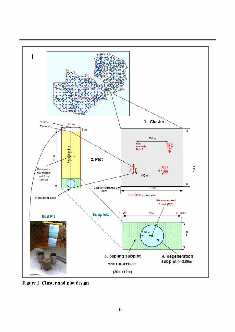
The sampling unit consists of five levels: 1) cluster, 2) plot for trees, stumps and fallen dead-wood 3) subplots for saplings and regeneration and 4) a soil pit for soil survey and 5) a quadrat for litter sampling. The design is as follows (see also Figure 1):

• Distance between new clusters varies. The cluster and plot coordinates are plotted on UTM map grid;

• A cluster is a square of 1 km x 1 km. The co-ordinates of the south-west corner of the clusters correspond to those of the points selected in the sampling frame.

• There are 4 plots in each cluster; plot locations fit on to the top of old ILUA I plots on ILUA II inventory sites (aka permanent clusters).

• Plots are rectangular, 20 m wide and 50 m long and they are numbered clockwise from 1 to 4 as shown in Figure 1. Trees with DBH>10 cm are measured in these plots as well as Stump and fallen deadwood measurements (for deadwood>10 cm DBH).

• Trees with 5cm < DBH < 10 cm are measured in a rectangular subplot which is 20 m wide and 10 m long. This subplot is located in the first 10 m of the larger plot from the starting point of the plot along the central axis.

• Regeneration subplot is a circular area with a radius of 3.99 m and one subplot is located within each plot. The regeneration subplot provides data about tree regeneration (i.e. about trees DBH< 5 cm). The center of the regeneration subplot is located 5 m off of plot starting point, along the central axis.

• Soils measurements are taken using a soils pit on all ILUA I clusters, and some ILUA II clusters that have been assigned as soils clusters.

• Litter samples are taken using a 0.5x0.5m quadrat along with a composite soil sample at the same location.

8

Figure 1. Cluster and plot design

9

Each plot is divided into land use/vegetation type sections (LUVS) representing homogenous land use or vegetation type units, with variable size and shape that have been identified in the field (Figure 2). The classification system adopted to identify the different classes is described in section 3. Most of the data related to forest characteristics and trees are collected within the LUVS. Note that the minimum area unit of a LUVS is 0.5 ha.

Figure 2. Example of land use/forest type sections (LUVS) distribution within a plot

There are 3 land use/ vegetation type sections in this plot, coded with letters A, B and C. The red lines indicate the limits between them. LUVS_A and LUVS_B belong to the same vegetation type.

Table 1. Survey unit specification

Unit name Shape Size (area) umber Corresponding

field form*

Cluster

1000 m x 1000 m (1 km2) One

F1

Plot

50 m x 20 m (1000 m2) Four per cluster

F2/F3

F5B for Trees

Subplot for saplings, 5 cm<DBH<10 cm

10 m x 20 m (200 m2) One per plot

F5A

Subplot for regeneration

Radius (r) = 3.99 m (50 m2) One per plot

F4

Soil Pit

mini-pit measuring 50 cm wide, 60 cm in length and

40 cm depth

One pit at Plot 1 for Soils Clusters

F8

10

Soil composite sample

Five composite soil samples will be obtained from the center of the sampling plot,

then five meters to the north, east, west and south

using the soil auger

Five composite samples for top soil (depth of 0-10cm) and sub-soil (depth of 10-30cm)

F8

Litter composite sample

1 meter to the north of the five composite soils

samples

Five litter samples using 0.5 m X 0.5 m quadrant that are individually weighed in the plot and one composite

sample

Five litter sample weights

and on composite sample

F9

Land Use/ Vegetation type Section (LUVS)

Variable depending on number of land

use/vegetation cover classes (covering 0.5ha in area) in

any given plot

At least one

F3/F5

* principal field form; note that units such as cluster, plot and LUVS will be required in multiple field forms

Table 2. Orientation of the plots

Plot Location of the starting point of the plot, within the 500 m inner

square Orientation Bearing

Plot 1 South-West corner South-North 0 / 360 degrees Plot 2 North-West corner West-East 90 degrees Plot 3 North-East corner North-South 180 degrees Plot 4 South-East corner East-West 270 degrees

The exact locations of sample plots are presented on a separate list and on the inventory field maps.

LUVS

1

LUVS

2

LUVS

3

11

2.3 Sample units

The primary sampling unit is a cluster of sample plots. The plots are grouped into clusters for practical reasons in order to take into account the reduced inventory costs and to match plots with ILUA I design. The measurement units, 4 plots, should be, as a rule of thumb, measurable within a working day by a field team, but on some sites the work may require a second working day. If some of the plots are outside forest, it may be possible to measure more than the target number. However, for difficult conditions it may take more time to accomplish the measurements. Sample plot information is collected in the plot area and some observations are also carried out on the plot’s surrounding area. Information for each individual plot is collected and recorded, some examples are land use, vegetation type, erosion, and human impact, as well as regeneration, fallen dead-wood, stumps and bamboos among others is collected. The inventory team will also collect data about the soil and litter on a preselected number of plots. For each tree inside the plot, the species name, the breast height diameter, the bole height, and the total tree height is accurately recorded. Most plot parameters are observed representing the plot area, but some parameters represent the surrounding area as well. The surrounding area is expected to be to some extent homogenous with the plot area with respect to the land use, vegetation type, accomplished measures or proposed future management (0.5 ha minimum). GPS measurements and other measurements and markings are done in such a way that re-measurement will be possible for quality control or future inventories.

3 Land use and vegetation type section (LUVS)

The land use and vegetation type section (LUVS), previously known as Land use/forest type section (LUS) in ILUA I, is recorded on all land types. If a plot is not accessible but the land use and vegetation type can be observed, this information needs to be completed on the field form.

The classification system used to define each land use/vegetation type section is based on a dichotomous approach and includes two levels:

- The first level is composed of the global classes designed for the assessment of forest and tree resources at the global level;

- The second level is country specific, and includes additional classes integrated to take into account national and sub-national information needs.

The global classes were developed within the framework of the Global Forest Resources Assessment of FAO. The terms and definitions used in national assessments are chosen to harmonize national with global level forest assessments. The global classes include:

- Forests;

- Other wooded land;

- Other land;

12

- Inland water.

The global classes ensure harmonisation of the classifications between countries for regional or global assessments. The second level of classification is designed to meet specific country needs of information.

ILUA II data collection will also inform Zambia’s efforts to Measure, Report and Verify (MRV) Greenhouse Gas (GHG) emissions from Deforestation and Degradation. Therefore, field data collection needs also to adhere to land use definitions established by the Intergovernmental Panel for Climate Change (IPCC) for GHG reporting. Broad land use definitions established by the IPCC are: Forest Land; Crop Land; Grass Land; Wetlands Settlements and Other Land. Note that the LUVS categorisation of Table 3 (Major Class Column) can be organised into the broad land use definitions established by the IPCC.

The land use/vegetation type section (LUVS) and related codes used in the ILUA are shown in Table 3. See also Annex 5 and 6 for more information. There is a 0.5 ha minimum area on each observed LUVS.

Table 3. Land use/vegetation type classification

Major

Land Use

Class (MLUC)

Definition of MLUC

(from FRA 2010) LUVS class Description

FOREST Area ≥ 0.5 ha

Tree crown cover ≥10%

Tree height ≥ 5 m

Dry evergreen forest Parinari forest and Copperbelt

chipya

Marquesia forest

Lake basin chipya

Cryptosepalum forest

Kalahari sand forest

Dry deciduous forest Baikiaea forest and deciduous

thicket

Itigi forest

Moist evergreen forest Montane forest

Swamp forest

Riparian forest

Forest woodlands Miombo woodland on plateau

Miombo woodland on hills

Kalahari woodland on sands

Mopane woodland on clay

Munga woodland on heavy soils

Forest plantations Broadleaved forest plantation

(Eucalyptus)

Coniferous forest plantation (Pine)

Other Area ≥ 0.5 ha

Tree canopy cover 5-10%

Wooded grasslands

Termitary vegetation and bush

groups

13

Wooded Land

Shrubs/bushes canopy

cover ≥10%

(Includes Dambo/plains

with sparse trees, cc 5-

10%)

Shrubs / Thickets

Other Land

Tree canopy cover <5%

or shrubs/bushes <10%

Grassland Dambos and Flood Plains

Marshland and Swamps

Bare land

Barren land

Sandy dune

Bare Rock / Outcrop

Cultivated and managed

land

Annual Crop

Perennial Crop (also includes groups

of fruit trees; canopy cover may be

greater than 5% in this instance)

Pasture Land

Fallow

Built-up areas Urban

Rural

Water Lakes Inland Water

Rivers

Dams

Other areas

Outside land area

(e.g.outside country)

4 Preparations for the fieldwork

This section of the manual includes recommendations on preparing and carrying out fieldwork activities. The fieldwork is described step by step for a sample plot, together with recommendations on the data collection techniques.

4.1 Overview of data collection process

Data is collected by field teams for sample plots. The main information sources for the assessment are: • Field measurements and observations in sample plots; • Remote sensing and map data.

Note that the house hold survey of ILUA I has been separated from biophysical assessments. The Forest Livelihood and Economic Survey (FLES), for which a separate manual is to be developed, will involve interviews with local people. The main part of this work will be carried out by the Central Statistical Office (CSO) as a separate survey, but there some variables on the biophysical field form

otice: The entire data collection process will be under the control of the Field Coordinator. This will be a member of the PMU stationed in the province where field

work is underway. All communication, and data collection forms will be transmitted

through the Field Coordinator.

14

which require information from local informants (i.e. question about Land tenure change, Forest products, and Human impact). Those two sources of information imply the use of different methods and approaches that complement each other. The process for data collection is summarized in Figure 3.

Figure 3. Data collection procedure

4.2 Field team composition and responsibilities

The field teams will be responsible for collection of data in the field and transmission of the field forms to Project Management Unit (PMU) for data entry and validation. The PMU is responsible of the nomination of the team members and the allocation of clusters for each team. The biophysical field team consists of the following members:

• Team leader; • 3 members to biophysical field measurements (enumerators). One team member is a botanist,

and one team member has skills in soil sampling. One team member is also nominated to act as assistant team leader;

• 1-2 local community members, if possible. (One can act also as assistant tree identifier); • Driver; • Game scout, as necessary.

15

At least two members should have forestry background and have experience in forest data collection. In order to collect information on the various land uses, the field team will be formed of at least one person familiar in this area of expertise. In addition, at least one member should also have good knowledge on soil data collection procedures. It is desirable that some members of the field teams are hired locally and act as guides and tree identifiers in the field. Additional persons may be included to improve performance of the field teams when conditions require greater resources, for example it may be necessary to carry camping items and to have a cook in the camp who will also secure camping facilities and valuable items. It is also advised to include forestry students for capacity building. The team leader and/or his assistant should identify the guide through the contact of local people. Responsibilities of the team members The responsibilities of each team member must be clearly defined. Their tasks are proposed as follows below. The team leader is responsible of the following tasks:

• Organizing all the phases of the fieldwork, from the preparation to the data collection, and planning the work schedule in an efficient way. He/she has the responsibility of contacting and maintaining good relationships with the community and the informants and has a good overview of the progress achieved in the fieldwork; he/she has the responsibility of maintaining harmony and good working spirit within the team;

• Contacting local forestry officers, authorities and the community. Introduce the survey objectives and the work plan to the local forestry staff and authorities, and request their assistance to contact the local people, identify informants, guides and workers;

• Specifically preparing for the fieldwork: carry out the bibliographic research, prepare field forms and collect the maps;

• Take necessary measurements and observations. The team leader is responsible for the quality of the work of team members.

• Taking care of logistics of the team: organize and obtain information on accommodation facilities; recruit local workers; organize access to the clusters;

• Filling in the forms and take notes; • Ensuring that field forms are properly filled in and that collected data are reliable; • Organizing meetings after fieldwork in order to sum up daily activities; • Organizing the fieldwork safety; • Submitting data to the PMU, soil and litter samples to the laboratory; • Submitting tree samples for identification; • Weekly updates on progress to the PMU.

The assistant of the team leader will: • Help the team leader to carry out his/her tasks; • Take necessary measurements and observations; • Make sure that the equipment of the team is always complete and operational; • Supervise and orient the workers; • Filling in the forms and take notes as required;

16

• Take-over in the team leader's absence.

The team members (enumerators) will carry out the field measurements. They measure/assess forest and tree attributes (tally and sample height trees, fallen dead-wood, stumps), regeneration data (i.e. number of tree seedlings), land use, vegetative cover and status. They also collect soil and litter samples. The botanist will focus on species identification, specimen collection, storage, and identification, and helping enumerators as time permits. The community members are assigned the following tasks, according to their skills and knowledge of local species, language and practices:

• Help to measure distances; • Clear vegetation to facilitate access and visibility for technicians; • Provide the common/local name of tree species; • Inform about access to the plots; • Provide information about the forest uses and management; • Carry the equipment and soil and litter samples; • Carry camping equipment and set up camp; • Cook.

The above description is simply the normal way of working, but it is not necessary to follow it exactly. Teams should choose their organization according to the specific skills and efficiencies of the team composition, optimizing for quality and time. Seedlings, sample height trees and dead-wood etc. can be measured by any capable team member. The driver is responsible for the vehicle and passengers, and he will guarantee the following:

• Take care of the vehicle maintenance and security; • Assure there is adequate fuel and extra fuel supplies when needed (using Jerry cans); • Help in loading and packing the equipment; • Ensure equipment is secure; • Transport the team members safety from and to the field; • Be ready in case of emergency.

4.3 Preparation phases

The preparation of fieldwork consists of the following phases: A. Bibliographic research; B. Preparation of the field forms and maps; C. Field Coordination responsibilities assigned;

otice: Team members must not litter on the sampling sites, on the trails or when parking their vehicle. ILUAII team members are

asked to carry out the trash that they carry in.

Let’s keep Zambia clean!

17

D. Quality Assurance Team established and activated; E. Soil survey and analysis coordinator activated; F. Field equipment (maintenance, checking); G. Contacts to provinces and local communities.

4.3.1 Bibliographic research

Auxiliary information is necessary to collect at the preparation phase. Existing reports on forest and natural resource inventories at the target area, farming systems, national policy and forestry community issues, local people, etc. have to be studied to enable the team members to understand and to build better knowledge on the local situation. If a target cluster is located in plantation forests, the forests’ history and management plans need to be examined, especially planting year and time of previous treatments are important details to be found. In many cases land use, user rights and forest ownership needs to be studied before going to the field.

4.3.2 Preparation of the field forms and maps

The PMU will ensure that the necessary field forms to cover the clusters are prepared and assigned to each team. The Team Leader must ensure that enough forms are available to carry out the planned field data collection. The forms are described in detail in Section 5. When revisiting ILUA I permanent plots, teams should be provided with the older ILUA I field forms in order to assist navigation and orientation to the plot start points. Detailed reference points and other necessary information are provided in these older forms which can be essential to relocating the older sites and finding the best accessible routes to the plots. Teams should be equipped with these forms and review them before they initiate field measurements. The use of secondary data sources, particularly maps and existing management plans, is necessary to determine information such as names of administrative centre (administrative maps), accessibility and forest ownership. Some sections of administrative data in the form may be filled in during the preparation phase, and be verified in the field. Maps and printed aerial photographs/satellite images covering the study area should be prepared in advance to help the orientation in the field. These may be enlarged and reproduced, if necessary, but a scale bar needs to be printed on maps. The plots’ locations in the cluster are to be indicated together with their respective coordinates in UTM-WGS84 (with respective UTM-zone number). Prior to the field visit, each team must plan the itinerary to access the cluster (e.g. using printed Google Earth images, road and topographic maps) which should be the easiest and least time consuming. Sample plot coordinates and topographic maps should be converted to GPS on the previous day before visiting the cluster. Advice of local informants (local forestry staff, for example) are usually valuable and help save time in searching the best option to access the cluster. An enlarged section of the map corresponding to the area surrounding the cluster will be prepared (photocopy or printed copy) and used to draw the access itinerary to the first plot.

18

Reference objects (roads, rivers, houses) that contribute to the better orientation of the team in the field should be identified during the planning phase. The numbers of the sample plots are entered into the GPS receiver according to following rule: [cluster number] + “P” (=Plot) + [Plot number] + “_S” (= Starting) OR “_E” (=Ending), e.g. for cluster 1443, plot 3, Starting point => 1443P3_S

4.3.3 Coordination of field work

A Field Coordinator from the Forestry Department will always be stationed close to the provinces where ILUA II field work is active. The designated Field Coordinator will coordinate all ILUA II field activities, and will be the first point of contact for field teams. The nominated Field Coordinator (to be nominated by the Forestry Department) will be the first point of contact for field teams. The Field Coordinator will be responsible for coordinating and executing all ILUA II field activities, and finally to collate, validate, and transfer all field data to the PMU. He/ she will provide the logistical support and supervision to the field (Forest Biophysical and FLES) personnel and to monitor, supervise, and provide backstopping support to the fieldwork including field report checks, in order to ensure timely completion for field work, data quality and homogeneity among field teams, The Field Coordinator should also facilitate the procurement and maintenance of field tools and equipment for ILUA II field teams, and provide immediate response and support to field teams if an emergency occurs. The Field Coordinator will also control and coordinate the data collection process, the transfer of field forms to the PMU, and the validation of field forms in preparation for data entry. The designated Field Coordinator will provide bi-weekly field work progress reports to the PMU.

4.3.4 Quality Assurance

A designated Quality Assurance (QA) team will ensure that the technical quality of ILUA II field measurements adhere to this manual. The QA team visits completed ILUA II clusters and undertakes a complete control measurement of Plot 1 for comparison with measurements from the field team. The QA team then examines the data collected by the field team relative to the control measurement and completes a checklist. A specific booklet for the QA team should be followed consisting of measurement sheets for plot 1, and a QA checklist. The control measurement of plot 1, and comparison should done in the cluster within weeks after the measurements of the ordinary team. The purpose of the control is to ensure that the team has done measurements according to the instructions detailed in this field manual and in a correct way. Furthermore, results of control measurements can be used for training purposes, that is, to find out issues which were unclear for the teams after training. Control measurement and checklist is for feedback and for making a conclusion report of all QA measurements in the reporting period. The QA team hands over the completed QA booklet to the field coordinator. Feedback is given both to the field team and field coordinator who is in charge of field work. The QA team goes through the observed shortcomings and errors of measurements with the ordinary field team in the feedback session. Differences in measurements between QA and field team are stated and unclear issues gone through.

19

The QA field team will consist of experts in the various disciplines (botany, soil science, forest inventory) required for ILUA II field work, and will consist of the following members:

• Team leader (inventory expert); • Soil science expert • Botanical expert • 1-2 local community members, if possible. (One can act also as assistant tree identifier); • Driver; • Game scout, as necessary.

4.3.5 Quality Assurance work flow

The Field Coordinator works in conjunction with the QA team to determine a timetable for control clusters. Field coordinator also hands over a copy of the original field forms filled by the ordinary field crews to the QA team. Usually QA teams get 10 clusters at the same time to be remeasured, approximately 1 cluster is visited per day. The feedback is given to the original field measurement team on the same day as the QA team visits the cluster when possible. The QA team leader decides which way the feedback is given, in a meeting or by phone. The differences, shortcomings and errors are gone through in the feedback session. Also reasons behind errors are discussed. Field coordinator decides if more control is needed for the crew. The implementation of control measurements is important for ILUA II Quality Assurance. The Quality assurance is especially important for field crews having new members and the feedback is a part of training. The field crews are able to correct the possible errors in their work when they get immediate feedback from the QA crew. The QA team must follow the instructions on the field manual and do the measurements carefully, and complete the QA Field Booklet for every visited cluster. The checklist should be filled in as instructed because they are used for reporting and for correcting measurement errors done by the teams. A separate QA Field Booklet has been created and should be followed and completed for every visited cluster and returned to the Field Coordinator.

4.3.6 Soil survey and analysis coordination

A soil survey and analysis coordinator will oversee all technical aspect of ILUA II soils collection, will coordinate (in conjunction with the field coordinator) the movement of samples (for soils, litter, and botanical samples) from the field to Forest Research in Kitwe. Coordination of soil survey field collection and laboratory analysis involves the following tasks: 1. Coordinate all analysis of soils in the soils laboratory at Forest Research in Kitwe 2. Ensure international standards of quality assurance for soils analysis 3. Maintain laboratory equipment 4. Maintain a ledger of incoming ILUA II soil samples and their status 5. Train laboratory assistants in analysis techniques for capacity building 6. Train graduates in soil survey techniques as a part of ILUA II field inventory

20

7. Assure quality assurance of ILUA II field soil survey 8. Coordinate the movement of soil samples from the field to the laboratory 9. Enter soils analysis results into the open foris collect tool at Forest Research 10. Create a monthly report of analysis undertaken and collate results for review by FD and FAO 11. Create a terminal report of work undertaken at the end of the contract for review by FD and FAO The following outputs are expected from the soil survey and analysis coordinator 1. Trained laboratory assistants in soils analysis techniques 2. Trained graduates in soil survey techniques 3. Technically cleared monthly reports of analysis undertaken 4. Soils data entered into Open Foris Collect 5. All analysis conducted to satisfy international quality assurance standards 6. Technically cleared terminal report at the end of the contract

4.3.7 Field equipment per team

The equipment needed by each field team are described in the following table.

Table 4. Equipment for field teams

Equipment needed umber

required

Comments

Measurement tools

Compass (360°) 1 In degrees

Water proof model

GPS receiver 1 + extra batteries + charger

Metal detector 1 For locating ILUA I plot markers

Measuring tape, 30 m 2 Metric, 1 cm units

Measuring tape, 50 m 1 Metric, 1 cm units

Diameter tape 1 mm scale

Caliper 1 mm scale

Laser Range Finder 1 For ranges, heights and angle

measurement

Suunto Clinometer 1 with 15m, 20m and % scales to

measure both tree height, in

meters; and slopes in percent.

Spherical crown densitometer 1 Canopy coverage measuring

equipment. Concave model.

Telescopic height measuring rod 1

Used for accurately measuring

bole and tree heights for small to

medium size trees

Waterproof bags As necessary

to protect measurement

instruments and forms

Disc Pasture Meter 1 Grass fuel load (biomass)

measurements

Soil auger 1 Soil auger has a fitting for

21

Equipment needed umber required

Comments

clay/wet soils and another fitting

for normal soils

Shovel 1 Used for excavating the soil pit

Pick-hoe 1 Used for excavating the soil pit

Munsell Soil Color Chart 1 Used for soil color assessment

Utility Pail 1 For collecting and mixing soil and

litter composite samples

Weight measuring scale 1 For measuring the weight of litter

samples

Soil sample ring kit 1 For collecting soil bulk density

samples from the soil pit

Zip seal plastic bags several For storing composite soil

samples

Measuring tape, 3m 1 For measuring soil depths of the

soil pit

Plastic measuring beaker 1 For measuring samples

Rubber mallet/hammer 1 Used to gently hammer the soil

core in the soil pit wall

Digital camera 1 For photographs of plots,

reference points, soil pit wall and

unknown species;

with extra batteries, and charger

Machete / Bush-knife As necessary

Pocket knife 1

30-50 cm long metallic pin As necessary Galvanized steel bars for plot

marking

Clothing

Boots and field outfit For permanent

team members

Helmet For permanent

team members

Should always be worn in

forested areas where there is

overhead vegetation

Rain coats As necessary

Gloves As necessary

Documents, papers Field forms As necessary Keep in plastic covers for rainy

days

Code check list with slope correction table

As necessary Needs to be laminated

Copies of ILUA I Cluster and Plot Forms or Database data tables

Field manual As necessary

Know your tree book As necessary

Topographic maps, field maps and printed aerial photo/satellite image

As necessary

22

Equipment needed umber required

Comments

Pencils and markers As necessary

Supporting board / writing tablet 1 To take notes

Hand calculator 1

Clipboard 2 To take notes

A4/A3 size flipchart 1 For photo identification

File Folder 1

Newspapers As necessary For collection of samples (plants/

leaves)

Other equipment (camping, security, communication)

Mobile phone At least 1 Not procured – use personal

mobile phone (credit will be

provided to the team leaders for

communications)

Radio phones 1+1 One for the field team, one for the

driver

Satellite phone 1 One for the team leader for

emergency use only

First aid kit 1 With phone numbers of hospitals

/ emergency

Flashlight and batteries As necessary

Camping equipment 1

Jerry can As necessary 5 Gallons (steel)

Rucksack As necessary 30 or 45 litters back packs; for

carrying and keeping filed forms

Water and food As necessary

The list of equipment is specified by measurement type in the following table.

Table 5. Equipment by measurement type

Measurement type / Activity Equipment required

PLOT Plot location determination GPS, maps, list of plot coordinates

Tree location determination 50m measuring tape, slope correction table,

compass, range finder

Plot marker establishment Metal pins, compass, measuring tape

Slope Suunto clinometer

Photo documentation Digital camera, flipchart

Canopy coverage Spherical densitometer

TREES Species name “Know your trees” book

Tree diameter 1.3 m stick; Diameter tape (mm scale)

Tree height Clinometer, 20/50m measuring tape

Bole height Clinometer, 20/50m measuring tape

STUMPS

23

Stump diameter Diameter tape

Stump height Measuring tape

FALLE DEAD-WOOD (CWD) Species name “Know your trees” book

Dead-wood diameters Caliper

Dead-wood length 20m measuring tape

Decay class Pocket knife

REGEERATIO Number of seedlings Fiberglass telescoping measuring rod,

measuring tape

BAMBOO Species code and name “Know your trees” book

Bamboo average diameter Diameter tape or Caliper

Bamboo average height Clinometer, 20/50m measuring tape

GRASS ABOVE GROUD BIOMASS Grass fuel loads Disc Pasture Meter

SOIL AD LITTER Digging the soil pit Pick-hoe, shovel, utility pail

Soil classification Munsell color chart

Soil bulk density samples Soil ring kit

Soil depth measurements 3m measuring tape

Composite soil samples Soil auger, utility pail

Litter sample Utility pail, and 0.5x0.5m quadrat from

measuring sticks (estimate quadrat using

0.5m twigs)

Litter weight Weight measurement scale

The condition of the inventory equipment needs to be verified prior to field work and missing or damaged items should be replaced with new or fixed tools.

4.3.8 Contacts

Each field crew, through its leader, should start its work by contacting GRZ district staff in the area where the clusters are located. These local staff may help contacting the authorities, community leaders and land owners in order to introduce the field crew and its programme of work in the area. The local staff may also provide information about access conditions to the site and about the people who can be locally recruited as guides or workers. They may also inform the local people about the project. A recommendation letter written by the Permanent Secretary for the Province, asking for support and assistance to the field crew members should be issued to facilitate the work. The information on the project activities will be broadcasted in the local radios if existing through a contact done by the Principal Extension Officer of FD.

24

4.4 Data collection in the field

4.4.1 Introduction of the project to local people

If the cluster area is inhabited, the team must establish contact with local people and on arrival to the site, meet with contacted persons and others, village representative, closest government institution, owners and/or people living in the cluster area. It is recommended to contact the local leaders well before visiting the area in order to inform or sensitize them of the visit and request permission to access the area. The team must briefly introduce and explain the aim of the visit and study. A map or an aerial photograph/satellite image, showing the target inventory area, may be useful to facilitate the discussion. It is important to ensure that both local people and the field team understand which area will be studied. The aim of the inventory must also be clearly introduced to avoid misunderstandings or raise false expectations. Cooperation and support from local people are essential to carry out the fieldwork. It is easier to achieve this support if the first impression is good. Nevertheless, it must be stressed that the fieldwork consists only of data collection and not local development or law enforcement project. Some key points about the project introduction are mentioned in the next text box.

Besides the presentation of the project, this initial meeting aims at resolving logistic matters. After the general introduction, access to the forest and other lands, as well as food and accommodation issues will be discussed.

Key points to be stressed during the presentation of the project to the local people are as follows:

• An objective of this assessment is to collect data on land uses to support national decision making by interacting with the local users. The collected land use information will be used by the country and the international community. The objective is to generate reliable information for improved land use policies that takes into account people’s reality and needs. Hopefully, this can lead to natural resources being managed in a sound and sustainable way. It could help also in the mitigation of poverty.

• The data are collected from two sources: (1) Measurements of the forests and trees outside the forests and other land use practices; (2) Interviews with local communities using land including forest users and other people who are knowledgeable of the area. This work will be carried out using the FLES tool implemented by the Central Statistical Office (CSO).

• Measurement examples to be mentioned may be: tree diameter and height, as well as forest species composition, fallen dead-wood, and soil carbon.

• Some of the clusters surveyed in the country will be monitored in the future, with the aim of assessing land use changes and development of forest resources.

25

IMPORTAT!

Plot coordinates are ALWAYS recorded using GPS reading,

they are NOT taken from the map or from the given list of plot

coordinates. Due to inaccuracy of any GPS model, recorded

coordinates are allowed to differ from the targeted location.

The team should aim to receive and record 3D measurement

only - thus receiving at least 4 GPS satellites’ signals.

4.4.2 Access to plot

The locations of plots will be pre-drawn on topographic maps. Clusters and plots are pre-numbered and provided on the inventory base map. Reference numbers of the plots are indicated on the printouts of topographic maps and maps within the GPS receivers. At the place of leaving the vehicle, the team records the accessibility of the cluster, the GPS coordinates of the vehicle, the date, the departure/start time, bearing and distance to 1st plot of the day, the plot to which they are headed and the time of return to the vehicle on the F1 Cluster Form. Orientation in the field will be assured with the help of a GPS unit where the locations of each plot’s starting point are registered as waypoints. In some cases a local guide will be useful helping to access the plots more easily. When revisiting ILUA I permanent plots, teams will be provided with the older ILUA I field forms in order to assist them in navigating and orienting to the plot start points. Detailed reference points and other necessary information are provided in these older forms which can be very helpful in relocating the older sites and finding the best accessible routes to the plots. Teams should be equipped with these forms along with topographic maps as reference material and review them before they initiate field measurements. Any difficulties faced in relocating the older plots or related reference points must be documented in the field forms in order to inform and assist future inventory teams.

4.4.3 Arrival at the plot

The position of the starting points of all 4 plots in the cluster needs to be precisely located, marked with a permanent marker (buried galvanized metal tube) if a new ILUA II cluster and properly referenced to facilitate relocation in the future.

For older ILUA sites, permanent markers need to be found in order to locate the exact starting point of the plot. A permanent marker should have been established for all of the ILUA I plot starting points, but in some cases field crews were not able to place markers in the ground at the exact starting point of the plot. The ILUA I field forms should indicate whether a marker was able to be established or not. Field crews should be able to locate permanent markers with the GPS unit and metal detector provided to each team. If field crews still experience difficulty with locating a permanent metal marker, they should refer to the older ILUA field forms which list the bearing and distances of references around the marker. The triangulation method can then be used to define the area where the marker should have

26

been installed. It helps if you clean the floor from all grasses, but do not destroy seedlings and saplings. Sometimes it is necessary after cleaning off the top soil to verify the location again using the triangulation method.

It is also important to use some previously measured trees on the plot to find the marker: these are the first trees measured in the plot. If the old marker is found, then marker data is filled in accordingly in Form F2 and the measurements within the plot can start. If the marker pin is not found within one hour, a new marker will be installed, and Form 2 marker data is filled in accordingly, and the measurements on the plot can start. The marker may not be able to be found if the land use class identified in ILUA I was cropland or if it was not well hidden and therefore removed. The older field forms can provide insight into the site conditions of the ILUA I plots and therefore can facilitate orientation to each plot starting point. If the marker is not able to be located, this must be recorded in F2-9, On all new plots, a permanent marker (i.e. galvanized metal pin) is placed into the ground. The marker pin must be placed exactly at the starting point of the plot. If for any reason (presence of rock etc.) the marker pin cannot be placed at the starting point, the permanent marker should be placed as close as possible to the starting point of the plot. Marker GPS location data must be collected together with a starting point description of the plot in order to enable relocation in the future. Regardless of whether the permanent marker can be placed at the starting point of the plot or not, three prominent reference objects (rock, largest tree, houses, etc) must be identified and the direction (compass bearing in degrees starting from the marker location) and distance from the marker should be measured (see Figure 5 and Table 6). A photo from the marker should be taken for each reference and coded (running photo number within Cluster). Photos should also be taken at the site of older ILUA references in order to inform on any changes which might have taken place since the last inventory. Note that GPS coordinates of reference points are not required if Marker point GPS coordinates can be recorded. For older ILUA plot locations, any notable changes in reference points or marker and starting position should be recorded. The starting point’s location data must be collected together with its description in order to enable relocation of the plot in the future.

27

Table 6. Example of recording the Reference points

D. Plot marker’s reference point data

From Marker to Reference Object 20.

Bearing [deg]

21.

Distance [m]

22.

DBH [cm]

for trees

23.

ID

Photo

24.

Remarks

ID 19. Type of object (if tree then give species)

1 North side of the rock 180 22 NA 28P2_R1

2 Anthill 280 53 NA 28P2_R2 at foothill

3 Baobab tree 87 40 116 28P2_R3

These indications are reported on a sketch (plot starting point plan, F2) where the reference points and the starting point of the plot are indicated.

If the GPS signal in a forest is poor due to dense canopy cover at the marker’s point (preferably the same location as the starting point) and GPS reading cannot be accessed, the team must record the GPS coordinates at the closest available position as the reference point and then measure the bearing and distance to the marker point.1 Distance can be measured with a range finder if there are no obstacles between the marker and reference point. Notice to follow these rules:

a) Starting point with marker:

1 Slope correction is obligatory when accessing the plot from the reference point with compass and measuring tape, as all distances refer to the horizontal

distance (use slope correction table provided in Annex 2 to adjust the distances). Note: If electronic range finder instruments are used for measuring distances, check the device settings that it automatically makes slope correction.

Figure 4. Location of marker and reference points in case of an obstacle at starting point

28

• The coordinates of plot marker position are determined with the help of GPS receiver (as averaging positions of several measurements). Then, an identification code will be assigned to identify each points measured by the GPS as follows:

[Cluster number] + “P” + [Plot number] + “_M” (=“Marker”), e.g. for cluster 113, plot 3 => 113P3_M

• A photo of the marker point may be taken, and it should show the same code; • A steel marker pin should be positioned in the ground at the starting point of all plots.

b) Reference objects for starting point: • Three prominent and preferably permanent reference objects (rock, non-abundant tree species

or largest tree, house etc.) as fixed points must be identified for a marker. • These objects should be 80-130 degrees apart to help with triangulation. • The following information is recorded about the reference point: object ID, type of object,

bearing (compass reading in degrees) to the plot marker, distance to the plot marker, tree diameter (if object is a tree), and photo ID.

• Reference point coordinates are only recorded if these cannot be measured at the plot marker point!

• A photo should be taken for each reference objects, and coded as follow: [Cluster number] + “P“ + [plot number] + “_R” + [running photo number within plot] (e.g. photo of the 3rd reference taken in the 2nd plot on the cluster number 28 => 28P2_R3

4.4.4 Data collection in the plots

The data collection starts at the plot starting point and continues in the predefined direction to the predefined distance. The progress along the central line will be made with the help of the compass and 50m tape. Measurements are carried out on the both sides of the central line on a 10m wide area. Rods or coloured ribbon will be placed on the corners of plots, corners of rectangular subplots and the border of the plot as the team advances in order to help the identification of the trees within the plot. Grass measurements are only carried out in all clusters. Ten measurements will be done using a Disc Pasture Meter in the plot. The use of Disc Pasture Meter is described in Annex 7. Different attributes are collected according to the data collection rules described in the next chapters.

Trees located at the border of the plot will be considered as inside the plot if at least half of the diameter of the stem base is inside the plot. If the stem centre is exactly on the plot limit then it will be considered alternately in and out (Figure 6). If a living tree is leaning, it is considered inside the plot if half of the base of its stem is inside the plot.

29

Borderline tree to be considered

inside

Borderline tree to be considered

outside

Inside tree

Plot central axe

Plot

The stem centre is exactly on the plot limit, but one such borderline

tree as already been included earlier so this one will be consider

outside and excluded

The stem centre is exactly on the plot limit, it is consider inside and

will be included

The stem centre is inside the plot, it will be included

The stem centre is outside the plot, it

will be excluded

4.4.5 End of data collection work on the plot and access to the next plot

Once the work on the first plot is completed, any flagging tapes are removed and the ending time is recorded in Form F2. The team walks to the next plot and if the forest cover allows, it is possible to directly access the new plot location with the help of the GPS. Otherwise, the team can use the compass and measure 450 m (horizontal distance) along the central line of the previous plot. If the starting point of the next plot to be reached is not accessible along a straight line, the obstacle must be bypassed using auxiliary methods that allow finding the original line (Figure 7).

Figure 6. Bypassing an obstacle during access to sample plot

4.4.6 Local Community Members as Key Informants

Some of the data essential to ILUA II will need to be collected through local community members who can provide local knowledge when completing the ILUA II field assessment (e.g. background information on the cluster, ownership & user rights, distance and access to the plots, forest products and services, etc.)

Figure 5. Borderline tree cases

30

4.4.7 Photos of the plot

Each inventory team uses the digital camera to record the view on the plot. There can be more than one photo of the plot. Photos will be used to document the plot characteristics as vegetation type, and to possibly enable the relocation of the plot in future reassessments. Photos should be taken from such

a place and way that the captured image illustrates the plot’s vegetation type in the best possible way. The camera setting should be set to Auto position, and with using wide focus. In any case, avoid taking photos against the sun light. The photo should include both some soil and vegetation, if possible. On private lands close to human settlements the team should ask for permission to take a photo. Whenever possible, one photo should be taken at the starting point location towards the plot axis. On that photo, the team should add a flipchart hanging on a tree with the following information: Cluster number, and Plot number. Similarly, a new photo should be taken if Land use/Land cover class changes inside of a plot. Data about each photo are recorded on the Plot Form. The team writes down the image ID Number in the camera’s memory stick. In the office the photos are transferred from the camera into a separate ‘<Province +ame> ILUA2 Photos’ folder, and where each photo is renamed as follows:

Cxxx_Pp_z.jpg Where xxx refers to cluster number, p refers to plot number, and z refers to order of image captured on the plot.

4.5 Soil and Litter Clusters

On specific clusters identified in the sampling plan, additional information is collected on soil and litter. Soil and litter clusters require additional measurements briefly described below, and the field teams must implement these measurements when clusters are identified as soil/litter clusters. Note that all ILUA I clusters are also soil/litter clusters.

4.5.1 Soil Pit

The position of the soil pit will always be placed 5m to the northern edge of the biophysical inventory sampling Plot 1. This is done to avoid undue disturbance in the sampling plots. The exact geographical location coordinates of the soil pit are determined with the help of GPS (The team should aim to receive and record 3D measurement only - thus receiving at least 4 GPS satellites’ signals). Once the soil pit has been dug a photograph will be taken of the soil pit with a graduated scale in cm placed against the wall of the exposed face to be sampled in the pit (0–10cm, 10–20cm and 20–30cm) as shown in Figure 8. If it is not practical for the soil pit to be located in the prescribed position due to certain physical obstacles (such as termite mounds, termitaria, river, surface rocks, buildings, roads ,etc.) being encountered, a reasonable alternative pit position should be determined and found as near as practically possible, and note made in remarks section of field sheet.

31

Figure 7. Example of a soil pit photograph

At the soil pit study site three types of soil samples will be taken. Firstly, the undisturbed core ring sample will be collected from the soil pit at 0–10, 10–20 and the 20–30cm layers, respectively. Secondly, from the same layers in the soil pit, disturbed soil samples are collected for the measurement of soil organic carbon in the laboratory. Thirdly, composite soil samples are prepared having been collected using a soil auger targeting the top soil (0–10cm), and sub soil (10–30cm depths) from within the sampling plot (at the biophysical plot centre and at 5m north, east, south and west). The soil pit dimensions will conform to a mini-pit measuring 50 cm wide, 60 cm in length and 40 cm depth. The soil pit is dug or excavated using hand tools like a hoe, pick or mattock and a spade. The width and length of the pit are just adequate to permit personnel to carry out soil morphological descriptions, collect the required soil samples for measurement of soil organic carbon. The orientation of the pit will be such that maximum light illumination falls on the vertical face of the pit prepared for description and sampling. The opposite side to this face will have a step-in stair-case-like arrangement of steps for the convenience of the soil sampler (Figure 9).

32

Figure 8. Diagram of soil pit size and depth

Once the soil pit has been dug a full soil description is undertaken and the following soil attributes are recorded; Soil colour using a Munsell soil colour chart; soil texture; soil structure and other soil attributes. For bulk density determination, undisturbed mineral soil samples are taken from the vertical side face of the pit using soil core rings for three depths; 0-10cm; 10-20cm; 20-30cm. Samples should be collected from the pit wall using a thick hard wood plank and short handled rubber hammer to insert the soil core vertically without side-ways movements or wobbling to avoid underestimate of bulk density, or an overestimate.

4.5.2 Surface plant litter sampling (Fine Litter)

Surface plant litter samples will be collected at the centre of plot 1, and then five metres north, east, south and west (see Figure 10). Use a 0.5m x 0.5m quadrat, and collect all the plant litter material debris within the square, weigh using an electronic balance and record the reading on the field record sheet. Fine litter consists of all debris above the soil with diameter less than 2cm. A quadrat can be created in the field using sticks and the 3 metre measuring tape. After each weight is taken, the materials from all the five positions are thoroughly mixed on a ground sheet, from which a ‘grab’ sample weighing approximately 1.0 kg is obtained, bagged, and labelled according to plot and cluster for transportation to the laboratory to determine the dry matter weight.

4.5.3 Fine Coarse Woody debris (CWD) Measurements

Fine CWD is all woody material with diameters between 2cm and 10cm. Fine CWD measurements involve a tally of similarly size woody material on the regeneration sub-plot (radius 3.99m).

33

4.5.4 Composite Soil Samples

Composite soil samples are to comprise disturbed soil samples collected in two ways, one from each of the soil pit layers sampled for bulk density, and another from within the sampling plot obtained from several spots collected at two levels, one topsoil (0–10 cm) and another, subsoil (10–30 cm) depths using the soil auger. These will be taken at the same location of litter samples after the collection of litter for weighing. By means of an auger, five (5) soil samples will be obtained from the centre of the sampling plot, then five meters to the north, east, west and south, as illustrated in Figure 10. Sample the surface or topsoil separately and place in a clearly marked container or bucket. Samples from the topsoil are combined and thoroughly mixed, from which a ‘grab’ sample, the composite sample is taken. This is about 500 g to 700 g soil material that is then placed into a clean sample bag, labelled according to location, depth for transportation to the laboratory. In a separate bucket the same procedure is repeated for the sub sample.

Figure 9. Locations of the Soil Pit and the Composite Soil Samples

4.5.5 Samples handling

All soil samples should be double plastic bagged, clearly labelled and stored in a dark cool stout box for transportation for laboratory analysis. Profile wall soil core rings are to be capped on both sides, and stored in the carry box for transport to the laboratory for processing. All litter samples should remain in staple-sealed paper bags, stored in large plastic containers for storage with lids to prevent ripping and water damage during transportation. Ensure the litter bags can ‘breath’ to prevent mould and water damage. This is done by perforating sample bags with a paper perforator.

4.5.6 Labels for soil and litter samples

Undisturbed and composite soil samples collected at different depths are to be labelled by province, district, cluster number, sampling plot, soil pit no. and depth of the sampling layer, with the date and name of sampler. Labels may be pre-printed prior to field work, with the required information details

34

to be completed whilst in the field. (see sample label details format in Table 9). Each sample must have a set of two labels written. One will be placed on the inside between the two double bagged sample bag, while the other will be placed, or tied on the outside of the bag for easy identification and sorting of samples. Litter samples are treated similarly, except the soil layer depth space or position will be marked “N/A”(not applicable). No blank spaces are permitted, so all spaces provided on the label should be filled and completed

4.5.7 Labels for bulk density core rings

Each bulk density core ring sample should be marked with adhesive label (such as that in Table 7) directly placed on the outside of the upper lid cap.

Table 7. Sample label detail format

SAMPLE TYPE ID

PROVINCE ID DISTRICT ID CLUSTER ID

SOIL PIT ID

SAMPLE No.

SOIL LAYER DEPTH

DATE SAMPLED

35

5 Description of field forms and variables

There are 9 different forms for biophysical data, as indicated below in Table 8.

Table 8. Field forms description and corresponding information level

Form o. Information

F1 Cluster: General information, time data, access to plot

F2 Plot: General plot description data, time data, marker position, plot level data

F3 LUVS and plot level data

F4 Regeneration data

F5 Tree measurements

F6 Stump data and Coarse Woody Debris (CWD)

F7 Bamboo data

F8 Soils

F9 Fine CWD and Litter

5.1 Form F1: Cluster

The Cluster Form 1 will be filled for each cluster. It contains general information about the cluster location and identification, the name list of persons involved in the assessment, distance to the main infrastructure, specification of equipment used, date of data collection, checking and entering data into the database. Description of the cluster form is given below. F1-1a. Cluster number

Cluster number from inventory plan. F1-1b. ILUA I - Cluster number

Old cluster number in ILUA I. F1- 2-5. Cluster location

General information on cluster location. a) Province name. b) District name. c) Township name. d) Village/locality name.

36

F1-6. ILUA I cluster

Y ILUA I cluster N New cluster

F1-7. Soil sampling cluster

Y Soil sampling cluster N Soil sampling not carried out in the cluster

F1-8. UTM Zone

UTM Zone used for GPS reading using UTM-WGS84 coordinate system. To be selected by marking the appropriate checkbox: 34, 35 or 36.

F1-9. Team Leader The name of the team leader. F1-10. Enumerator The name of the individual team member writing down the inventory data F1-11. GPS Model

GPS Model: brand name and type. F1- 13-19. Proximity distance to infrastructure (km)

From the centre of the cluster, record road distance (in km) to a) All-weather road. The closest all-weather road (accessible by motor vehicle all the year),

departing from the tract centre (equal to 0 if the road is located within the cluster). b) Seasonal road. The closest seasonal road (road accessible by motor vehicle during some

seasons only). c) Settlement. The closest inhabited area. d) Health institution. The closest health facility. e) School. The closest school. f) Food Market. The closest food market (to satisfy domestic needs). g) Input Market. The closest agriculture and forestry market (seeds, fertilizers, forestry tools,

etc.) F1-20. Accessibility

Condition of accessibility is recorded for each cluster.

Code Description

0 Accessible 1 Inaccessible due to slope

2 Inaccessible due to owner refusal; owner does not allow one enter the site

3 Inaccessible due to restricted area; e.g. military or border areas 4 Inaccessible due to water body

37

99 Inaccessible due to other reason; specify in Remarks F1- 21-22. Vehicle parking point GPS reading (m)

Easting UTM system coordinate (in meters) Northing UTM system coordinate (in meters)

F1- 23;29. Plot (to access)

The plot number to which the team aims to walk. F1- 24;30. Date

Date when work in the cluster started (day/month/year). F1- 25;31. Time of leaving from vehicle

time when leaving the vehicle to access the first plot of the cluster by foot (hour : minutes) during the first and/or second measurement day.

F1- 26;32. Bearing from vehicle parking point to the Plot 1 (m)

Compass bearing (from 0 to 360 degrees) from the vehicle to the Plot 1 starting point. F1- 27;33. Distance from vehicle parking point to the Plot 1 (m)

Distance (in meters) from the vehicle to the Plot 1 starting point. F1- 28;34. Time of returning to vehicle

End time of measurement in the plot (hour : minutes) at the first and/or second measurement day.

F1-37. Remarks

Additional remarks and notices about the cluster or access to the plot.

Follow up of raw data

After the field work is over and the field forms are filled in, the raw data will be delivered to the PMU through a project officer. The following data will be filled in:

a) Name of the person who delivers the raw data after the end of the field work. b) Name of the person who receives the raw data. c) Date of the raw data delivery.

Follow up of data

a) Control team leader name b) Date of control c) Name of the person who enters the data into the database d) Date of data entry e) Name of the person who validates the data f) Date of data validation

38

F2

5.2 Form F2: Plot

Plot Forms 2 and 3 will be filled in for each plot contained in the cluster. The forms will include the general data on the plot and the information on its location and access. Some data are filled in by Land use/vegetation type sections (LUVS). Regardless of accessibility, each plot is expected to have a

field form F2 and F3 F2-1. Cluster number

Cluster number from inventory plan. F2-2. Plot number

Plot number within cluster from inventory plan. PART A. Time record within the plot F2-3a. Date 1

Date when measurements on the plot are conducted (day/month/year). F2-4a. Arrival time 1

Time when team arrives at the plot (hours : minutes) at the first measurement day. Time entered is that when crews first arrive at plot, before searching for marker.

F2-5. Time to locate the old Marker (minutes)

If the old Marker is found, record the total time needed to locate this Marker (minutes). F2-6a. End time 1

End time of measurement in the plot (hours : minutes) during the first measurement day. F2-3b. Date 2

Second date when measurements in the plot are done (day/month /year). This is filled in if the work in the plot cannot be completed within one day.

F2-4b. Arrival time 2

Time when team arrives at the plot (hour : minutes) during the second measurement day.

F2-6b. End time 2

End time of measurement in the plot (hour : minutes) at the second measurement day. PART B. Plot starting point, marker position and ending point F2-7-8. Plot marker point GPS reading

39

F2

Easting UTM/WGS84 system coordinate (in meters) Northing UTM/WGS84 system coordinate (in meters)

+OTE. If the old Marker is not found, record this position to the new Marker. F2-9. Old Marker found

Information whether ILUA I plot marker is found in the field. Y Yes

N No +OTE: If the marker is not found after one hour active searching, establish new marker and start measurements.

F2-10. ew Marker installed

Y Yes N No F2-11. Marker at starting point

Y Yes N No

F2-12. Bearing from Marker to Plot starting point

Compass bearing (from 0 to 360 degrees) from marker to the plot starting point. This data is equal to “0” if the marker and the starting point coincide.

F2-13. Distance from Marker to Plot starting point (m)

Distance (in meters) from the plot starting point to the marker. This data is equal to “0” if the marker and the starting point coincide.

PART C. Plot accessibility and slope data F2-14. Slope along plot axis

Slope along plot axis is recorded from the plot starting point and refers to the overall slope of the plot in relation to the plot axis. Unit is percent. See Slope Correction Table in Annex 4 for conversion from degrees to percentage.

F2-15. Slope

Slope is recorded from the plot starting point as average of two measurements towards uphill and downhill in the direction of maximum slope. Unit is percent. See Slope Correction Table in Annex 4 for conversion from degrees to percentage.

F2-16. Slope bearing

40

F2

Slope bearing is recorded to the direction of the maximum slope, at the plot starting point. Slope azimuth is recorded with the compass (360 degrees). If there is no slope on the plot, then this field can be left as blank.

F2-17. Remarks

Additional information about the plot. PART D. Plot marker’s reference point data

Reference point ID

Identification IDs for four reference points are in the F2 field form (R1,R2,R3,R4). At least three reference objects are required!

F2-18 a-d. Type of object

Name of the fixed point’s object; e.g. stone, rock, tree and tree species. F2-19 a-d. Bearing from Marker to Reference Point

Orientation of the reference points from the marker F2-20 a-d. Distance from Marker (m) to Reference Point

Distance (in meters) from the marker to the reference point of interest

F2-21 a-d. Diameter (of reference tree) (cm)

Diameter The diameter of the reference tree in cm, one digit (0.1 cm). NA Not applicable. Reference object is not a tree.

F2-22 a-d. Photo ID

The photo ID corresponding to the reference. Read more at 4.4.7 Photos of the plot. F2-23 a-d. Remarks on references

Additional information about reference object or location of the measurement point. F2-24 a-b. Plot reference point GPS reading (m)

Plot reference point GPS reading are recorded only if the marker point coordinates cannot be measured. Easting UTM/WGS84 system coordinate (in meters) Northing UTM/WGS84 system coordinate (in meters)

PART E. Plot ending point and Sketch map displaying plot layout. F2-25. Plot end point GPS reading (m)

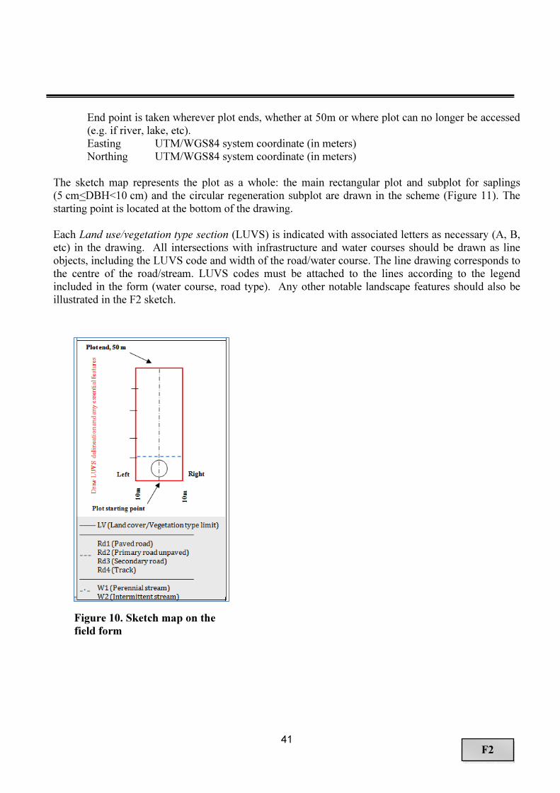
41

F2

End point is taken wherever plot ends, whether at 50m or where plot can no longer be accessed (e.g. if river, lake, etc). Easting UTM/WGS84 system coordinate (in meters) Northing UTM/WGS84 system coordinate (in meters)

The sketch map represents the plot as a whole: the main rectangular plot and subplot for saplings (5 cm<DBH<10 cm) and the circular regeneration subplot are drawn in the scheme (Figure 11). The starting point is located at the bottom of the drawing. Each Land use/vegetation type section (LUVS) is indicated with associated letters as necessary (A, B, etc) in the drawing. All intersections with infrastructure and water courses should be drawn as line objects, including the LUVS code and width of the road/water course. The line drawing corresponds to the centre of the road/stream. LUVS codes must be attached to the lines according to the legend included in the form (water course, road type). Any other notable landscape features should also be illustrated in the F2 sketch.

Figure 10. Sketch map on the field form

42

F3

5.3 Form F3: LUVS/plot data

5.3.1 Data collected in the plot and surrounding area

Information on Land use/vegetation type section (LUVS) found in a given Plot will be registered on this form. It contains general data related to the LUVS as well as data on forest structure and management and on agriculture management, product and services. One form is used to record

information on each LUVS. Minimum area unit on any given LUVS is 0.5 hectares. The following variables are recorded both in the plot area and observed also by viewing the properties of the similar lands surrounding the plot. F3-1. Cluster number

Cluster number from inventory plan. F3-2. Plot number

Plot number within cluster from inventory plan.

5.3.2 Land use/vegetation type section (LUVS)

The following variables are recorded in the plot section (LUVS) areas. Part A: To be completed in all land use/vegetation type sections for each individual land use/veg. type section F3- 3. Section code

Code indicates the Land use/vegetation type section inside of the plot. The plot is shared into several sections in case it contains more than one land use or vegetation types.

A Section where the plot’s starting point locates B The second section C The third section (etc.) F3- 4. Land Use/Vegetation Type Section (LUVS) In LUVS

Land use/ vegetation type section (LUVS) is recorded on ALL land types. It refers to the dominant land use purpose for humans and vegetative cover at the time of observation. Land use is observed within the plot’s outer boundary, along the plot centre line. If a plot contains more than one land use/vegetation type, each land use type requires a new plot form to be completed. If a plot is not accessible but the land use/vegetation type can be observed, this information needs to be completed on the field form. In the case of inaccessible areas where the LUVS cannot be specified, write “nk” (=”not know”) in the box. THIS DATA MUST BE COMPLETED.

43

F3

See also Annex 5 and 6 for more information.

Code Description Major class

Forest 01 Parinari forest and Copperbelt chipya Dry evergreen forest

02 Marquesia forest

03 Lake basin chipya

04 Chryptosepalum forest

05 Kalahari sand forest

06 Baikiaea forest and deciduous thicket Dry deciduous forest

07 Itigi forest

08 Montane forest Moist evergreen forest

09 Swamp forest

10 Riparian forest

11 Miombo woodland on plateau Forest woodlands

12 Miombo woodland on hills

13 Kalahari woodland on sands

14 Mopane woodland on clay

15 Munga woodland on heavy soils

16 Broadleaved forest plantation

(Eucalyptus)

Forest plantations

17 Coniferous forest plantation (Pine)

Other Wooded Land 21 Termitary vegetation and bush groups Wooded grasslands

22 Shrubs / Thickets

Other Land

31 Dambos and Flood Plains Grassland

32 Marshland and Swamps

33 Barren land

Bare land

34 Sandy dune

35 Bare Rock / Outcrop

36 Annual Crop Cultivated and managed land

37 Perennial Crop (includes stands of fruit

trees)

38 Pasture Land

39 Fallow

40 Urban Built-up areas

41 Rural

Water, o vegetation

50 Inland Water

90 Outside land area (e.g. outside country)

44

F3

F3-5. Accessibility In LUVS

Condition of accessibility is recorded for each LUVS. If a plot is not accessible but the land use, land cover or ownership types can be observed in the field or detected from other sources (as from maps or aerial photos/satellite images), these data are completed on the field form, but observation method is explained in Remarks.

Code Description

0 Accessible

1 Inaccessible due to slope

2 Inaccessible due to owner refusal; owner does not allow one enter the site

3 Inaccessible due to restricted area; e.g. military or border areas

4 Inaccessible due to water body

99 Inaccessible due to other reason; specify in Remarks

F3- 6a. LUVS width (m) In LUVS

Average width of the LUVS in meters within the plot

F3- 6b. LUVS length (m) In LUVS

Average length of the LUVS in meters within the plot F3 – 7. Designation / Protection status: In LUVS

Protection status and legal/official designation. To be indicated according to option list:

Code Description Explanation

0 Strict nature reserve/ Wilderness area

Protection/Conservation

1 National Park

2 Natural monument

3 Habitat/ species management area

4 Protected landscape / seascape

5 Gazetted national and local forests

Multiple Purpose 6 Game Management Areas

7 Other Multiple Purpose

8 Production Indigenous Production

(Includes concessions, exploitation

licences, community forests etc.) 9 Production Exotic

90 Not known No information available

99 Other To be specified in the notes

45

F3

F3- 8. Fire occurrence In LUVS

Fire occurrence is recorded in all vegetation types.

Code Description Explanation

0 No There is no evidence of fire

1 Recent fire Evidence of fire during the current season/year

2 Old fire Evidence of fire during the previous years but not during current season

F3- 9. Fire area In LUVS

Surface area of fire in the LUVS within the plot. To be indicated in m².

F3- 10. Fire type In LUVS

(multiple choice possible):

Code Description Explanation

0 Not applicable

1 Underground fire Fire spreading under the surface through roots or any other

underground means

2 Surface fire Fire spreading through the ground cover where it consumes litter and

ground vegetation without reaching the tree canopies

3 Crown fire Fire spreading through the canopies of woody vegetation

F3- 11. Environmental problems In LUVS

Main environmental problems observed/identified within the LUVS. To be indicated by marking the appropriate checkbox. May also be asked or cross checked with observations or information provided by external key informant: (multiple choice possible).

Code Description Explanation

0 Not applicable E.g. Urban areas

1 Not existing No environmental problems

2 Loss of water levels in rivers

and other sources When the main resources of water use have dried up

3 Drought Continuous periods of dry weather that usually affects

agriculture, other human activities and climate

4 Flooding Seasons where a large quantity of water covers an area

5 Poor water quality When the water quality does not meet needs of the

population

6 Pests When pests start affecting plants in the area

7 Erosion

When excessive soil is carried away in the landform to

the extent that gullies and other erosion signs can be

observed

8 Loss of soil fertility

When nutrients of soil are being reduced to the extent

that the crop yields are reduced due to intensive use of

chemical inputs, soil erosion, poor soil management

practices

46

F3

9 Burning Fire that has expanded and become difficult to extinct

10 Landslide Mass movement of land resulting in the collapse of the

hillsides

11 Wind throw Including storms, cyclones…

12 Overexploitation of forest

resources

When a resource its used in a way that its natural

recuperation its not enough to maintain it

13 Overgrazing Excessive loss of herbaceous vegetation cover due to

wildlife or livestock grazing

14 Invasive species When exotic species start growing and affecting native

species in the area

15 Salinization When there is soil and groundwater degradation

through salt intrusion

16 Fungus When there is excessive fungal activity affecting plants

in the area

90 Not known

99 Other To be specified

F3- 12. Intensity of Environmental problem In LUVS Intensity of each associated environmental problem.

Code Description

1 Low

2 Medium

3 High

4 Very high

F3- 13. Grazing Intensity In LUVS

Grazing intensity is recorded in all vegetation types. Grazing refers to the impact animals have on forage growth and reproduction and on soil and water quality2. Animals do not have to be present on the plot at the time of the observation, but that signs of grazing are an adequate indicator of the presence of this activity.

Code Description Explanation

0 No grazing There is no evidence of grazing

1 Occasional Only choice plants and areas show use.

There is no use of poor forage plants.

2 Frequent Most range shows use. 1/3 – 2/3 of

primary forage plants showing use.

3 Extensive

Lands can be severely hedged. There is

evidence of livestock trailing to forage.

More than 2/3 of primary forage plants

showing use.

2 See e.g. Holechek & Galt (2000).

47

F3

F3-14. Livestock Management In LUVS

Livestock production system – recorded in all vegetation types. Key informants may have to assist with this question if not captured through observation alone. Multiple choice response possible.

Code Description Explanation

0 Not Applicable No presence nor trace of cattle in plot

1 Communal grazing

2 Fenced unimproved pastures

3 Fenced Improved pastures

4 Tethering Animals tied to a tree or peg

90 Not Known

99 Other To be specified in Remarks

Part B. Forest and Other wooded Land management and structure F3- 15. Stand origin In LUVS (Forests & OWL)

To be indicated by marking the appropriate checkbox (multiple choice possible):

Code Description Explanation

N Natural Natural regeneration of stand by seed

P Plantation Artificial regeneration by seeding or planting

C Coppice Regeneration by shoots from stump or roots

NK Not known

F3- 16. Planting year In LUVS (Forests & OWL)

Planting year is recorded in Plantation forests only, if this information is available. Information sources e.g. forestry documents and plans. Year is recorded as number in 4 digits, e.g. 2007.

48

F3

F3- 17. Stand structure In LUVS (Forest & OWL)

Distinct canopy layers in the stand. To be indicated according to an option list:

Code Description Explanation

0 Not applicable Non forest area

1 Single layer Stand with only one well-defined layer

formed by the tree canopies

2 Two-layer vegetation

Stand with two distinct canopy layers, an

upper layer (a dominant canopy layer with

two thirds above the lower layer, forming

a clearly defined layer with at least 20%

cc) and a lower layer (under storey).

3 Three-layer vegetation

Stand with three distinct canopy layers

each with at least 20% cc:

- a dominant upper layer two thirds above

the lowest layer.

- an intermediate layer where the canopies

is from one to two thirds above the lower

layer.

- a lowest layer (under storey) growing at

a maximum height of one third of the

dominant layer

F3- 18. Canopy coverage In plot (Forest)

Canopy coverage is recorded on Forest vegetation types where canopy cover is greater than or equal to 10%. Canopy coverage caused by trees is measured using the spherical densitometer at three plot locations (10, 25, and 40m along the plot axis). If coverage is caused for instance by banana leaves, these are not recorded as canopy cover. The measured value will be recorded in the form. Counts of the filled square areas at three points along the plot axis are each recorded on the field form.

F3- 19. Undergrowth In LUVS (Forest & OWL)

Undergrowth is recorded on Forest and OWL vegetation types. Undergrowth refers here to the dominating type of brush (small trees, bushes, or grasses) growing beneath taller trees in the forest. Code Description Explanation

0 No undergrowth

1 Bushes

2 Grass

3 Elephant grass

4 New tree generation

5 Mixed of bushes, grass, herbs or new

tree regeneration

Neither is clearly dominating alone

99 Other vegetation To be specified in Remarks

49

F3

F3 –20 Shrub coverage In LUVS (Forest & OWL)

Vertical projection of the shrub canopies as percentage of the total ground area. To be indicated according to option list:

Code Description

0 Not applicable

1 <10%

2 10-40%

3 40-70%

4 >70%

F3- 21.Tree/Forest Management proposal In LUVS (Forest & OWL)

Management proposal is recorded on Forest and Other Wooded Land vegetation types. The proposed action is suggested to be done during the next 3 years. This information is used to estimate the potential amount of silvicultural and sustainable harvesting activities to be done on forest lands, both in natural or planted stands. Multiple choice possible.

Code Description Explanation

0 No treatment

1 Selective cutting (commercial)

2 Selective cutting (domestic use)

3 Thinning

Reduction of trees within a plantation to

allow for the development of desired future

trees e.g. In the case of plantation

4 Clear felling

5 Law enforcement E.g. actions due to illegal activities

6 Change designation status E.g. productive to protective or vice versa.

Explain in Remarks.

7 Pruning To cut away some of the branches to improve

the tree bole quality

8 Coppicing Cutting the main stem to allow regeneration

9 Pollarding Cutting branches of a tree routinely for fodder

or fuelwood

10 Cleaning /Weeding Intervention aimed at freeing trees from

disturbing vegetation layer (e.g. lianas)

11 Enrichment Planting

Supplementary planting or seeding of certain

tree species for increasing the percentage of

desirable species

12 Sanitary cutting

Removal of dead, damaged or unhealthy

trees, with the aim of stopping or preventing

the spreading of insects and diseases

13 Early burning e.g. controlled burning

50

F3

14 Boundary maintenance

99 Other Specify in remarks

F3- 22. Disturbances In LUVS (Forest & OWL)

Impact level of human activity in the forest or other wooded land. To be indicated according to option list:

Code Description Explanation

1 Not disturbed Protected areas, all resources conserved

2 Slightly disturbed Exploitation of goods and services is carried out according to

management plans

3 Moderately disturbed Many products collected without conforming to management

plans, notion of sustainability not respected

4 Heavily disturbed

Heavily disturbed (removal of products at rates higher than

Mean Annual Increment (MAI), biodiversity degradation due

to high pressure on selected species, encroachment of

agriculture leading to high rate of deforestation

F3- 23. Timber extraction In LUVS (Forest & OWL)

Tree harvesting system applied in the LUCS. To be indicated by marking the appropriate checkbox. Multiple choice possible:

Code Description Explanation

0 No felling No recent felling observed

1 Clear-cutting Clear felling. All or almost all trees in

a stand have been harvested

2 Seed tree cutting

The majority of trees are cleared from

a stand with a few select ones

remaining as seed trees

3 Single tree selective cutting

Selective felling extracting only trees

of certain species, dimensions, quality,

value, etc.

4 Group felling Extraction of groups of trees

5 Strip felling Extraction of strips of trees

90 Not known

99 Other To be specified

51

F3

F3 – 24. Silviculture In LUVS (Forest & OWL)

Visible silvicultural practices (cutting). To be indicated by marking the appropriate checkbox. Multiple choice possible:

Code Description Explanation

0 No silvicultural practice No visible silvicultural practice

1 Pruning To cut away some of the branches to improve the tree shape,

bole and wood quality

2 Thinning Reduction of trees to allow for the development of desired

future trees

3 Coppicing Tree stems are repeatedly cut down at or near at the ground to

allow many new shoots to emerge from the stump

4 Pollarding

The growth of new lateral branches is encouraged by cutting tree

stem above the ground (usually 2 or 3 meters) or main branches.

Pollarding is maintained through regular pruning

5 Enrichment planting/seeding

– Indigenous sp

Supplementary planting or seeding of indigenous species for

increasing the percentage of desirable species

6 Enrichment planting/seeding

– Exotic sp

Supplementary planting or seeding of exotic species for

increasing the percentage of desirable species

7 Cleaning /Weeding Intervention aimed at freeing trees from disturbing vegetation

layer (e.g. lianas)

8 Sanitary cutting Removal of dead, damaged or unhealthy trees, with the aim of

stopping or preventing the spreading of insects and diseases

9 Prescribed burning

Controlled application of fire to vegetation in either their natural

or modified state, under specified environmental conditions

which allow the fire to be confined to a predetermined area and

at the same time to produce the intensity of heat and rate of

spread required to attain planned resource management

objectives

10 Fire break

Creation and maintenance of a discontinuity in the forest stand

in order to stop or reduce fire intensity and effectively control it

at specific points

99 Other To be specified

5.3.3 Crop production and management

Part C. This section should be filled out only for LUVS classified as cultivated and managed land (annual crops, perennial crops, pasture land and fallow fields).

It contains information on products provided by the land as well as on crop management. Most of the information will be collected through observations and possibly through interviews with farmers.

F3- 25. Cropping system In LUVS (Other Land)

This section should be filled out only for LUVS classified as cultivated lands. A cropping system describes how crops are managed. Multiple choice possible

52

F3

Code Description Explanation

1 Multiple cropping Cultivation of two or more crops on the same field in a year. Sole or

mixed crops are grown in sequence, simultaneously one after

another, or with an overlapping period

2 Improved

cultivars

From research, extension, private sector not from local participatory

breeding

3 Crop rotation Different crops are grown in sequence, one after another in a field in

unit time e.g. rice-wheat annual rotation

4

Fallow A period during the year, the land is kept bare and no crop is raised

on it, usually between one or more main crops. Conventionally

thought to provide a "resting" period to the soil in order to enable it

to recuperate

5 Monoculture Growing of the same crop year after year on a given piece of land

6 Mixed cropping

The system of raising two crops in the same field at the same time

where the crops are either broadcast seeded together, or grown as a

mixture within a row without any definite planting/spacing pattern

unlike intercropping

7 Intercropping

The growing of two or more crops on the same field, either

simultaneously or - in the case of relay intercropping - with an

overlapping period. Simultaneous systems refer to the cultivation of

two or more crops either intermingled or with distinct row or strip

arrangement

8 Mixed

crop/livestock Mixed crops with livestock

9 Agroforestry

Refers to land use systems and technologies in which woody

perennials (trees) are deliberately raised with herbaceous plants,

cultivated crops and/or animals on the same land

10 Shifting

cultivation

The growing of crops for a few years on selected and cleared plots

alternating with a lengthy period of vegetative fallow when the soil

is rested. Cultivation consequently shifts within an area that is

otherwise covered by natural vegetation.

90 Not known There is not enough information to know about the cropping system

99 Other To be specified in Remarks

F3- 26. Current and recent crops In LUVS (Other Land)

Categories of crops cultivated in the LUVs during the past one year (including current crops). Note: one line for each product category. To be indicated according to option list and according to importance if more than one crop. Multiple choice possible.

Options Description/definition Code

Annual

cro

ps

pro

duct

s

Food crops

Upland rice Not permanently flooded and previously forest has

been cut 1

Swamp rice In flooded areas also known as lowland rice 2 Sesame 3 Maize 4

53

F3

Findo 5 Millet Includes bulrush and finger millet 6 Sorghum 7 Beans 8 Groundnuts 9 Sweet potatoes 10 Irish potatoes 11 Cassava 12 Sugar cane 13 Vegetables 14 Bisab Wonjo 15 Other annual

food crop To be specified 91

Non-food crops Cotton 16 Other non-food

annual crops To be specified 92

Per

enn

ial

crop

s

Fruit trees Mango trees 17 Guava trees 18 Citrus trees 19 Papaya trees 20 Avocado trees 21 Soloumplum 22 Banana 23 Other fruit trees

To be specified 93

Other perennial crops

Jatropa 24 Oil Palm 25 Coconuts 26 Cola nut 27 Cashew nut 28 Other perennial crops

94

Agroforestry species Acacia sp 29 Leucaena sp 30 Gmelina 31 Moringa 32 Other

agroforestry

species

To be specified 95

54

F3

F3- 27. Soil and water conservation In LUVS (Other Land)

Practices for protection against erosion and for soil and water conservation. To be indicated by marking the appropriate checkbox. Multiple choice possible:

Code Description Explanation

0 None

1 Levelling Reduction of sloppiness of the land

2 Contour farming Field operations, such as plowing, planting, cultivating, and

harvesting are done along the contour

3 Terracing Terracing of the land

4 Crop residue

incorporation Crop residues are left on the soil to become part of the organic matter

5 Cover crops /

vegetation Maintenance of dense vegetation to prevent soil from erosion

6 Mulching

Material such as straw, plant residues, leaves, stubbles, loose soil or

plastic film is placed on the soil surface to reduce evaporation and

erosion, suppress weeds and protect plant roots from extremes of

temperature

7 Windbreak Trees planted on strips to protect crops from the wind

8 Grassed waterway /

Check dams

Strips of grass seeded on in areas of cropland or small, temporary or

permanent dam constructed across a drainage ditch or channel,

aiming at reducing the rate of water flow or at preventing severe

erosion

9 Tree planting /

Agroforestry Tree planting for soil and water conservation

90 Not known There is not enough information to know about the soil and water

conservation

99 Other To be specified in Remarks

F3- 28. utrient application In LUVS (Other Land) Use of fertilizer or other soils amendments. Multiple choice possible.

Code Description Explanation

0 None

1 Adequate fallow Soil quality improved by allowing enough fallow period

2 Organic fertilizers Soil quality improved by use organic fertilizer

3 Mineral fertilizers Soil quality improved by use inorganic fertilizer

4 Liming Soil quality improved by liming

90 Not known There is not enough information to know about the

nutrients for soil amendment

99 Other soil amendments To be specified in Remarks

55

F3

5.3.4 In the Plot

Part D. Data in this section is to be recorded inside the plot area in all LUVs. F3- 29. Ownership In plot

Ownership is recorded on all land types. Ownership refers here to the right to exclusively use, control, transfer, or otherwise benefit from a forest. Ownership can be acquired through transfers such as sales, donations, and inheritance. Note that formally, all trees in Zambia are owned by the State, regardless of the ownership of the land, however, you should ask your local informant for this information, as ownership of the forest will vary at the local level.

If a plot is not accessible but the ownership type can be observed, this information needs to be completed on the field form.

Code Description Explanation

1 Private individual Owned by individuals and families

2 Private industries Owned by private enterprises or industries

3 Others private

Owned by private co-operatives, corporations, religious and

educational institutions, pension or investment funds, NGOs, nature

conservation societies and other private institutions

4 Public. State Owned by central government, or by government-owned institutions

or corporations

5 Public. Local

government

Owned by local government (district, municipalities)

6 Customary

Owned by a collective, a group of co-owners, a community who hold

exclusive rights and share duties. Owned by indigenous or tribal

people

90 Not known No information available on the land ownership

99 Other To be specified in Remarks

F3- 30. Recent change in land tenure? In plot

Land tenure change presence: Have there been changes in tenure of the land the plot falls in during the last 10 years?

Code Description Explanation

N No No, there has been no change in tenure

in sample area

Y Yes Yes, changes in tenure have occurred in

the sample area

NA Do not know / Data not available Interviewee is uncertain if changes in

tenure have occurred in the sample area

F3- 31. Past ownership (status) In plot

56

F3

Past tenure status: If changes in land tenure have occurred, from which type of ownership did they shift?

As Ownership codes (F3- 24a)

F3- 32. Presence of a formal management plan In plot and surrounding area

Information about presence of a formal management plan in the area. Y Yes N No NA No information.

F3- 33. Seasonality In plot

Seasonality is recorded on all land types.

Code Description Explanation

1 Dry Dry season (generally occurring between April and October)

2 Rainy Rainy/Wet season (generally occurring between November and

March)

F3- 34. Grass biomass (Disc Pasture Meter) In plot

Above-ground standing grass biomass is measured using the Disc Pasture Meter and it is recorded in all LUVs types. The measurements are conducted in 10 randomly selected plot locations. See Annex 7 for instructions.

F3- 35. Biodiversity In plot and surrounding area

Specify recorded species or other special characteristics if possible. Digital photos of rare forest objects can also be captured (make notice in Remarks). Interviews with the community members will be necessary to get this data, but it can also be observed by looking for scat and/or tracks. The information about biodiversity may help us to locate new important biodiversity ‘hotspots’ and to target more detailed surveys into those areas. There are three data input fields in the field form to record this variable. Multiple responses allowed.

Code Description Explanation

0 No data None of the following ever observed by

informant

1 Big mammals Lion, elephant, rhino, etc

2 Other mammals

3 Reptiles

4 Birds

5 Insects Specify e.g. butterflies, beetles

6 Caterpillars

7 Climbers, Lianas, Rattan

8 Reeds, Phragmites, Papyrus Reed= tall, grass-like plant of wet

57

F3

places.

Phragmite = large perennial grass found

in wetlands.

9 Bamboo

10 Cactuses, Succulent plants

11 Alien invasive plant species Specify these

12 Plants (excluding those listed above)

13 Epiphytes

Epiphyte is a plant that grows upon

another plant (such as a tree) non-

parasitically

14 Parasitic plants

15 Bryophytes (Lichens, Mosses)

16 Fungus

17 Rare biotope e.g. springs, montane, rock outcrops,

riparian

99 Other To be specified

F3- 36. Biodiversity status In plot and surrounding area

Specify occurrence/abundance in the plot and surrounding area.

Code Description Explanation

0 Not applicable Variable is not countable, e.g. rare

biotope

1 Low abundance

Species are observed only once or

twice.

In case of plants, these do not cover

much of the area.

2 Medium abundance

Several species/cases are recognized.

In case of plants, these cover less than

one fourth of the area

3 High abundance

Multiple species/cases are recognized.

In case of plants, these cover more than

one fourth of the area

F3-37. Remarks/ otices on Biodiversity In plot and surrounding area

Additional information or specifications for biodiversity variables. F3- 38. Forest and tree products/services In plot and surrounding area (in LUVs)

Forest products/services are recorded in all land use/ vegetation types. These data refer to wood products, non-wood forest products (NWFP) and services provided by the trees, forest and other wooded land. Interviews with the community members will be necessary to get this data. Multiple responses allowed. There are five data input fields in the field form to record the most important forest products/services.

58

F3

Code Description Explanation

0 No data

1 Wood products Industrial wood Includes timber, chips

2 Fuelwood

3 Charcoal

4 Wood carvings

11 NWFP Fruits, nuts, seeds, roots,

berries, etc

Vegetable foodstuffs and beverages

provided by fruits, nuts, seeds, roots, etc.

12 Mushrooms Foodstuffs provided by mushrooms.

13 Fodder Animal and bee fodder provided by leaves,

fruits, etc.

14 Rattan

15 Plant medicines

Medicinal plants (e.g. leaves, bark, roots)

used in traditional medicine and/or for

pharmaceutical companies.

16 Herbs and spices

17 Dying / tanning

Plant material (bark and leaves) providing

tannins and other plant parts (especially

leaves and fruits) used as colorants.

18 Seeds Seeds collected for regeneration purposes

19 Other plant products Specify in Remarks

20 Wildlife Provides habitat for wildlife

21 Beekeeping activities

(e.g.Honey) Products provided by bees

22 Caterpillar Important collection areas

31 Forest services and

benefit Windbreak Acts as a windbreak

32 Shade Provides shade

33 Aesthetic Provides landscape beauty

34 Recreation and tourism

potential

Including ecotourism, hunting or fishing as

leisure activity. Unique feature.

35 Cultural heritage

potential Including religious / spiritual potential

99 Other Specify in Remarks

F3-39. Ranking of Forest products/services In plot and surrounding area

Ranking of the product or service according to importance.

Code Description Explanation

0 Not applicable

1 Low Products of low importance

2 Medium Products of medium importance

3 High Products of high importance

59

F3

F3-40. Species/Varieties

Local or scientific name of species in the product category, harvested in the land use class (one line per species/ varieties). If a local name is used then the language used to name the species should be specified into brackets. If several species have very similar characteristics (see following variables), they can be noted in the same row.

F3- 41. User rights In plot

User rights to harvest forest products (by product category and only to forest products)

Code Description Explanation

1 Individual rights The harvester is the land owner or has been transferred

property rights

2 Rent Pays a fee, percentage of harvest….for having the right

of harvest the product

3 Harvesting license/Permit Pays a fee for harvesting the product

4 Land lease Pays a fee for leasing the land

5 Customary or common rights

Rights to harvest the product based on tradition or

habit, to satisfy local people’s needs or a specific

group. Might be regulated through permits and licenses

6 Open access The harvest of the product is a common right.

Everybody has the right to harvest/use the product.

7 No right The harvest of the product is prohibited

90 Not known There is not enough information to know about the user

rights

F3- 42. Remarks/ otices on Forest products/services In plot and surrounding area

Additional information or specifications for forest products/services variables. F3- 43. Remarks

Additional information about plot and/or LUVS section.

60

F4

5.4 Form F4: Tree regeneration and shrubs

Tree regeneration and shrubs are recorded in all vegetation types in Form 4 (F4), and is collected on one circular, 3.99 m radius subplots. The data is collected on all seedlings, saplings and shrubs with DBH less than 5 cm. F4- 1. Cluster number

Cluster number from inventory plan. F4- 2. Plot number

Plot number within cluster from inventory plan. F4-3. LUVS code

Land use/ vegetation type section (LUVS) in regeneration subplot. F4- 4. Species name

Scientific genus and species name are recorded. As a last resort, when the scientific name cannot be derived, local name may be written, but the language must be clearly stated

F4- 5. Language

Language of local species name. F4- 6. umber of saplings, seedlings, shrubs in DBH class

Count of saplings and seedlings by species and diameter classes, 1 cm intervals. F4- 7. Remarks

Additional information about regeneration and shrub plot. .

61

F5A

5.5 Form F5A: Saplings

Measured only on the sapling subplot; first 10 meters of the full plot. Tree data are recorded by Land use / vegetation type sections (LUVS) in Form F5A.

F5A- 1. Cluster number

Cluster number from inventory plan. F5A- 2. Plot number

Plot number within cluster from inventory plan. F5A- 3. LUVS code

Land use/vegetation section code (A, B, etc.) F5A- 4. Sapling number

Sapling number, starting from number 1 on each plot. F5A- 5. Previous sapling number (ILUA I) (if available)

Sapling number needs to be reconciled against ILUA 1 measurements to detect changes over time.

F5A- 6. Species name

Scientific genus and species name are recorded. As a last resort, when the scientific name cannot be derived, local name may be written, but the language must be clearly stated. If species is completely unknown, a sample for the herbarium must be collected following instructions in Annex 9. enter ‘Unknown’ followed by the specimen number noted on the collected sample.

F5A- 7. Language

Language of local species name: B= Bemba, N= Nyanja, K= Kaonde, L= Lozi, T= Tonga, Lu= Lunda, Lve=Luvale

F5A- 8. Location along plot axis (m)

Horizontal distance in meters along the plot axis from plot starting point to the tree (from 0 to 10m).

F5A- 9;10. Location along left or right axis (m)

Horizontal distance in meters from the plot central axis to the tree (from 0 to 10m). F5A- 11. Sapling diameter, DBH (0.1cm)

Sapling diameter is measured above bark in centimetres, with 1 decimal digit, at 1.3m breast height above the ground with the exception of particular cases mentioned at page 79. The diameters are measured above bark.

62

F5A

F5A- 12. Height of DBH measurement (0.1m, default value: 1.30m)

Height of DBH measurement if it is not 1.30m. Record this data as required due to stem enlargement or buttress.

F5A- 13. Bole height (0.1m)

Bole height refers to merchantable or utilizable height that is defined as the distance from the base of the sapling to the first occurrence of the lowest point on the main stem, above the stump, where utilization of the stem is limited by branching or other defect. Bole height is recorded for all saplings.

F5A- 14. Use of sapling

The main use of sapling is recorded on all standing saplings.

Code Description Explanation

0 No usable / Not applicable

1 Saw logs and timber

2 Poles

3 Fuel wood / Charcoal

4 Medicinal use

5 Fruits

99 Other uses Specify in Remarks

F5A- 15. Quality

Quality status of bole or stem is recorded on all standing live trees.

Code Description Explanation

1 Straight stem Good quality. The entire bole length is

straight or on average circular in shape.

2 Bend stem Bole is slightly bent but sawable

3 Crooked stem Bad form, crooked bole which cannot

be sawn

F5A- 16. Health

Health status refers to the current observed condition of a sapling and the main causal agent. Health status is recorded on every sapling.

Code Description Explanation

1 Healthy

A tree is healthy when it does not show

symptoms of disease or other agents

that have had any substantial effect on

the tree’s growth and vitality. Excludes

63

F5A

burned trees.

2 Compromised

The tree is compromised when its

growth and vitality are diminished

(because of termites, past minor fire

damage etc.)

3 Severely affected

The tree is severely affected when it

shows symptoms that substantially

affect the tree’s growth and vitality

without being lethal

4 Dying A tree is dying if it shows damage that

will surely lead to death

5 Dead

A tree is dead when none of its parts are

alive (leaves, buds, cambium). Must be

standing, otherwise recorded as

“deadwood”

F5A- 17 Causative agents: Causative agents that have been identified (diseases, insects, animals, etc.) according to option list (multiple choice possible):

Code Description Explanation

0 No Damage Healthy tree crown, with no symptoms

or signs of

1 Insects

Evidence of insect infestation ( e.g.

defoliation, leaf feeding)

2 Disease/Fungi Presence of fungus such as leaf spots,

leaf or needle discoloration

3 Fires Disturbance caused by fire

4 Animals Damage due to wild or domestic

animals

5 Humans Human induced damage (cuttings, bark

damage,logging...)

6 Climate Damage caused by extreme climatic

events (wind, snow, lightning, etc.) e.g.

broken branches

90 Not Known Cause of damage cannot be determined

99 Other To be specified in Remarks

F5A- 18. Damage severity

A damage severity parameter is recorded adjacent to the Damage code. Damage severity is an estimate of the prevalence of damages to the live trees, and it is needed to predict future mortality. If substantial numbers of living trees are classed as very severely damaged (class 3), mortality is likely to remain high for a long time.

64

F5A

Code Description Explanation

0 No No damages

1 Slight Slight: Evidences of damages are visible, but does not qualify for serious

2 Serious

Serious: > 33% of the roots or boles with > 33% of the circumference

affected; damage > 33% of the multiple-stems (on multi-stemmed

woodland species) with > 33% of the circumference affected; > 33% of the

branches affected; damage > 33% of the foliage with >50% of the

leaf/needle affected.

3 Very serious

Very serious: > 66% of the roots or boles with > 66% of the circumference

affected; damage > 66% of the multiple-stems (on multi-stemmed

woodland species) with > 66% of the circumference affected; > 66% of the

branches affected; damage > 66% of the foliage with >50% of the

leaf/needle affected.

F5A- 19. Origin

This parameter describes the origin of a tally tree. ‘C’ should be use for coppicing trees, regardless of whether they are originally naturally occurring or planted. On afforested sites, please remember to add the code for ‘Afforestation’ on the Plot Form (Human impact).

Code Description Explanation

N Natural Natural regeneration of stand by seed. Default value if this field is left

blank

P Planted Artificial regeneration by seeding or planting

C Coppice Regeneration by shoots from stump or roots

Nk Not known

F5A- 20. Total height (0.1m)

Total height is measured from the seeding (base) point to the top of the sapling. If the seeding point is higher than the ground level (e.g. in case where a tree growing on the top of a stone), the sapling height is measured from the seeding point.

65

F5B

5.6 Form F5B: Trees

Tree data are recorded by Land use / vegetation type sections (LUVS) in Form F5B.

F5B- 1. Cluster number

Cluster number from inventory plan. F5B- 2. Plot number

Plot number within cluster from inventory plan. F5B- 3. LUVS code

Land use/vegetation type section code (A, B, etc.) F5B- 4. Tree number

Tree number, starting from number 1 on each plot. F5B- 5. Previous tree number (ILUA I) (if available)

Tree number need to be reconciled against ILUA 1 measurements to detect changes over time. F5B- 6. Species name

Scientific genus and species name are recorded. As a last resort, when the scientific name cannot be derived, local name may be written, but the language must be clearly stated. If species is completely unknown, a sample for the herbarium must be collected following instructions in Annex 9. enter ‘Unknown’ followed by the specimen number noted on the collected sample.

F5B- 7. Language

Language of local species name: B= Bemba, N= Nyanja, K= Kaonde, L= Lozi, T= Tonga, Lu= Lunda, Lve=Luvale

F5B- 8. Location along plot axis (m)

Horizontal distance in meters along the plot axis from plot starting point to the tree (from 0 to 50 m).

F5B- 9;10. Location along left or right axis (m)

Horizontal distance in meters from the plot central axis to the tree (from 0 to 10m). F5B- 11. Tree diameter, DBH (0.1cm)

Tree diameter is measured above bark in centimetres, with 1 decimal digit, at 1.3m breast height above the ground with the exception of particular cases mentioned at page 79. The diameters are measured above bark.

66

F5B

F5B- 12. Height of DBH measurement (0.1m, default value: 1.30m)

Height of DBH measurement if it is not 1.30m. Record this data as required due to stem enlargement or buttress.

F5B- 13. Bole height (0.1m)

Bole height refers to merchantable or utilizable height that is defined as the distance from the base of the tree to the first occurrence of the lowest point on the main stem, above the stump, where utilization of the stem is limited by branching or other defect. Bole height is recorded for all trees.

F5B- 14. Use of tree

The main use of tree is recorded on all standing trees.

Code Description Explanation

0 No usable / Not applicable

1 Saw logs and timber

2 Poles

3 Fuel wood / Charcoal

4 Medicinal use

5 Fruits

99 Other uses Specify in Remarks

F5B- 15. Quality

Quality status of bole or stem is recorded on all standing live trees.

Code Description Explanation

1 Straight stem Good quality. The entire bole length is

straight or on average circular in shape.

2 Bend stem Bole is slightly bent but sawable

3 Crooked stem Bad form, crooked bole which cannot

be sawn

F5B- 16. Health

Health status refers to the current observed condition of a tally tree and the main causal agent. Health status is recorded on every tree.

Code Description Explanation

1 Healthy

A tree is healthy when it does not show

symptoms of disease or other agents

that have had any substantial effect on

67

F5B

the tree’s growth and vitality. Excludes

burned trees.

2 Compromised

The tree is compromised when its

growth and vitality are diminished

(because of termites, past minor fire

damage etc.)

3 Severely affected

The tree is severely affected when it

shows symptoms that substantially

affect the tree’s growth and vitality

without being lethal

4 Dying A tree is dying if it shows damage that

will surely lead to death

5 Dead

A tree is dead when none of its parts are

alive (leaves, buds, cambium). Must be

standing, otherwise recorded as

“deadwood”

F5B- 17 Causative agents: Causative agents that have been identified (diseases, insects, animals, etc.) according to option list (multiple choice possible):

Code Description Explanation

0 No Damage Healthy tree crown, with no symptoms

or signs of

1 Insects

Evidence of insect infestation ( e.g.

defoliation, leaf feeding)

2 Disease/Fungi Presence of fungus such as leaf spots,

leaf or needle discoloration

3 Fires Disturbance caused by fire

4 Animals Damage due to wild or domestic

animals

5 Humans Human induced damage (cuttings, bark

damage,logging...)

6 Climate Damage caused by extreme climatic

events (wind, snow, lightning, etc.) e.g.

broken branches

90 Not Known Cause of damage cannot be determined

99 Other To be specified in Remarks

F5B- 18. Damage severity

A damage severity parameter is recorded adjacent to the Damage code. Damage severity is an estimate of the prevalence of damages to the live trees, and it is needed to predict future mortality. If substantial numbers of living trees are classed as very severely damaged (class 3), mortality is likely to remain high for a long time.

68

F5B

Code Description Explanation

0 No No damages

1 Slight Slight: Evidences of damages are visible, but does not qualify for serious

2 Serious

Serious: > 33% of the roots or boles with > 33% of the circumference

affected; damage > 33% of the multiple-stems (on multi-stemmed

woodland species) with > 33% of the circumference affected; > 33% of the

branches affected; damage > 33% of the foliage with >50% of the

leaf/needle affected.

3 Very serious

Very serious: > 66% of the roots or boles with > 66% of the circumference

affected; damage > 66% of the multiple-stems (on multi-stemmed

woodland species) with > 66% of the circumference affected; > 66% of the

branches affected; damage > 66% of the foliage with >50% of the

leaf/needle affected.

F5B- 19. Origin

This parameter describes the origin of a tally tree. ‘C’ should be use for coppicing trees, regardless of whether they are originally naturally occurring or planted. On afforested sites, please remember to add the code for ‘Afforestation’ on the Plot Form (Human impact).

Code Description Explanation

N Natural Natural regeneration of stand by seed. Default value if this field is left

blank

P Planted Artificial regeneration by seeding or planting

C Coppice Regeneration by shoots from stump or roots

Nk Not known

F5B- 20. Total height (0.1m)

Total height is measured from the seeding (base) point to the top of the tree. If the seeding point is higher than the ground level (e.g. in case where a tree growing on the top of a stone), the tree height is measured from the seeding point.

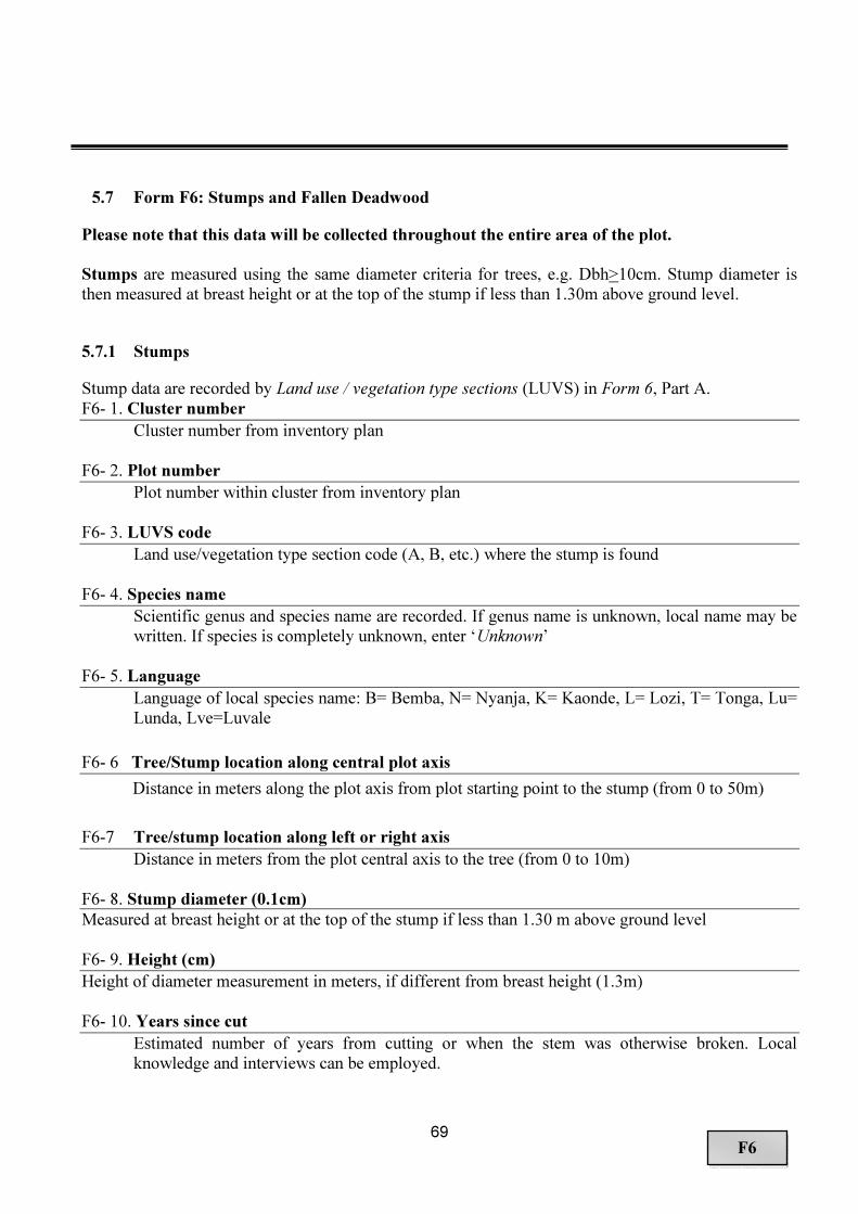
69

F6

5.7 Form F6: Stumps and Fallen Deadwood

Please note that this data will be collected throughout the entire area of the plot. Stumps are measured using the same diameter criteria for trees, e.g. Dbh>10cm. Stump diameter is then measured at breast height or at the top of the stump if less than 1.30m above ground level.

5.7.1 Stumps

Stump data are recorded by Land use / vegetation type sections (LUVS) in Form 6, Part A. F6- 1. Cluster number

Cluster number from inventory plan F6- 2. Plot number

Plot number within cluster from inventory plan F6- 3. LUVS code

Land use/vegetation type section code (A, B, etc.) where the stump is found F6- 4. Species name

Scientific genus and species name are recorded. If genus name is unknown, local name may be written. If species is completely unknown, enter ‘Unknown’

F6- 5. Language

Language of local species name: B= Bemba, N= Nyanja, K= Kaonde, L= Lozi, T= Tonga, Lu= Lunda, Lve=Luvale

F6- 6 Tree/Stump location along central plot axis

Distance in meters along the plot axis from plot starting point to the stump (from 0 to 50m)

F6-7 Tree/stump location along left or right axis

Distance in meters from the plot central axis to the tree (from 0 to 10m)

F6- 8. Stump diameter (0.1cm)

Measured at breast height or at the top of the stump if less than 1.30 m above ground level F6- 9. Height (cm)

Height of diameter measurement in meters, if different from breast height (1.3m) F6- 10. Years since cut

Estimated number of years from cutting or when the stem was otherwise broken. Local knowledge and interviews can be employed.

70

F6

Code Description Explanation

1 < 1 year ago

2 1-5 years ago

3 6-10 years ago

4 >10 years ago

5 Not known

5.8 Fallen dead-wood/Coarse woody debris

Please note that this data will be collected throughout the entire area of the plot. Dead-wood data are recorded by Land use / vegetation type sections (LUVS) in Form 6, Part B. In this section, data are recorded on fallen dead logs and branches with a diameter equal to or above 10 cm and which are found in the plot area (regardless of where they originated). Minimum length of dead-wood to be measured is 1 meter. Note, combined broken parts (separately shorter than 1 m) from the same tree are counted and measured as one if total length of parts exceed 1 meter. The length and diameter at both ends of all pieces of fallen wood with diameter larger or equal to 10 cm within the plot area are measured. Measurements of length are made to the plot border. Standing dead trees are measured as normal tally trees. F6- 11. LUVS code

Land use/vegetation type section code (A, B, etc.) F6- 12. Species name

Scientific genus and species name are recorded. If genus name is unknown, local name may be written. If species is completely unknown, enter ‘Unknown’.

F6- 13. Language

Language of local species name. F6- 14. Diameter 1 (cm)

Diameter at the stump part of stem in centimeters (dbh >10cm) F6- 15. Diameter 2 (cm)

Diameter at the top part of stem in centimeters (dbh >10cm) F6- 16. Length (0.1 m)

Length of wood part in meters with one decimal digit. (length >1m) F6- 17. umber of similar stems/parts

71

F6

Number of similar size dead-wood parts (species, diameter 1, diameter 2, length and decay). F6- 18. Decay

Decay refers to the decomposition of wood substance caused by the action of wood-destroying fungi, resulting in softening, loss of strength and mass. S Solid wood material R Fully or partially rotten wood material

72

F7

5.9 Form F7: Bamboo

This form contains information related to bamboo clumps (all bamboo shoots taller than 1.3 m). Bamboo data is recorded on all vegetation types, whenever applicable. The average diameter is at the breast height (1.3 m above ground). Dead and alive bamboos are recorded separately, when possible. Bamboo data are recorded by Land use / vegetation type sections (LUVS) in Form 7. F7- 1. Cluster number

Cluster number from inventory plan F7- 2. Plot number

Plot number within cluster from inventory plan F7- 3. LUVS code

Land use/vegetation type section code (A, B, etc.) F7- 4. Species name

Scientific genus and species name are recorded. If genus name is unknown, local name may be written. If species is completely unknown, enter ‘Unknown’.

F7- 5. Language

Language of local species name. F7- 6. Status

A= Alive D= Dead

F7- 7. Average diameter (cm)

Diameter at the breast height (1.3m above ground) of mean size bamboo stem. F7- 8. Average height (0.5m)

Mean height of bamboo culms. F7- 9. umber of stems

Number of bamboo stems in clump.

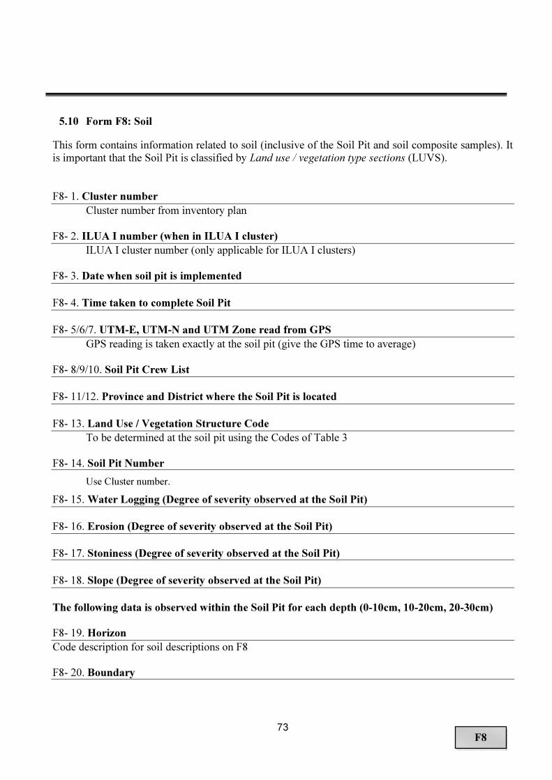
73

F8

5.10 Form F8: Soil

This form contains information related to soil (inclusive of the Soil Pit and soil composite samples). It is important that the Soil Pit is classified by Land use / vegetation type sections (LUVS). F8- 1. Cluster number

Cluster number from inventory plan F8- 2. ILUA I number (when in ILUA I cluster)

ILUA I cluster number (only applicable for ILUA I clusters) F8- 3. Date when soil pit is implemented

F8- 4. Time taken to complete Soil Pit

F8- 5/6/7. UTM-E, UTM- and UTM Zone read from GPS

GPS reading is taken exactly at the soil pit (give the GPS time to average) F8- 8/9/10. Soil Pit Crew List

F8- 11/12. Province and District where the Soil Pit is located

F8- 13. Land Use / Vegetation Structure Code

To be determined at the soil pit using the Codes of Table 3 F8- 14. Soil Pit umber

Use Cluster number.

F8- 15. Water Logging (Degree of severity observed at the Soil Pit)

F8- 16. Erosion (Degree of severity observed at the Soil Pit)

F8- 17. Stoniness (Degree of severity observed at the Soil Pit)

F8- 18. Slope (Degree of severity observed at the Soil Pit)

The following data is observed within the Soil Pit for each depth (0-10cm, 10-20cm, 20-30cm) F8- 19. Horizon

Code description for soil descriptions on F8 F8- 20. Boundary

74

F8

F8- 21. Coarse material

F8- 22. Colour

The colour of the soil matrix of each horizon should be recorded in the moist condition (or both dry and moist conditions where possible) using the notations for hue, and chroma values as given in the Munsell Soil Color Charts. F8- 23. Mottles

F8- 24. Texture

Soil texture refers to the proportion of the various particle-size classes (or soil separates, or fractions) in a given soil volume and is described as soil textural class. The names for the particle-size classes correspond closely with commonly used standard terminology. See Annex 10 for a description of soil texture determination. F8- 25. Structure

F8- 26. Consistence

F8- 20. Moisture

F8- 20. Compactness

F8- 26. Voids

F8- 20. Roots

75

F9

5.11 Form F9: Litter and Fine Coarse Woody Debris

Litter and Fine CWD are recorded only on soils clusters using Form 9 (F9), and are collected on one circular, 3.99 m radius subplots. The data is collected on all coarse woody debris with DBH less than 10cm, but greater than or equal to 2cm. Coarse woody debris less than 2cm diameter is included in the Fine Litter collection. F9- 1. Cluster number

Cluster number from inventory plan. F9- 2. Plot number

Plot number within cluster from inventory plan. F9 -3. LUVS code

Land use/vegetation type section code (A, B, etc.) F9 -4. Litter weights for five 0.5x05m quadrates

Litter weights measured accurately in the field using a weight measurement scale F9 -5. Litter Composite Sample Label

Label used to identify composite litter sample for identification in the laboratory F9- 6. CWD diameter, DBH (0.1cm)

CWD diameter is measured at the mid-point above bark in centimeters, with 1 decimal digit. F9- 7. CWD Length

Height of DBH measurement if it is not 1.30 m. Record this data as required due to stem enlargement or buttress.

F9- 8. umber of similar stems/parts

Number of similar size dead-wood parts (diameter, length and decay). F9- 9. Decay

Decay refers to the decomposition of wood substance caused by the action of wood-destroying fungi, resulting in softening, loss of strength and mass. S Solid wood material R Rotten

76

Annex 1. Cluster Selection and Distribution

In Zambia, a double sampling for stratification (Neyman 1938) has been proposed, where for the first phase; 6283 observations were distributed systematically across the country with an interval of 0.1 degrees (approximately equal to 10 km, see Figure 12). For each observation, using a special tool developed by FAO, and the Google Earth Platform, variables such as percentage of tree cover, land use/cover, and vegetation cover were evaluated from 1 hectare square.

Figure 11. Google Earth sampling frame

Points on the top of bare land, built-up land, and water were left out from the second phase sampling population. Based on consultations with the national stakeholders and national consultants, each primary observation was classified into one of the defined strata described as follows:

1. Stratum: Grassland, Other Wooded Land (OWL), Forest with crown cover <10%; 2. Stratum: Forest with crown cover >80%; 3. Stratum: Forest with crown cover >50% and <80%; 4. Stratum: Forest with crown cover >10% and <50%; 5. Stratum: Forest, Dry / Moist evergreen; 6. Stratum: Forest, Dry deciduous; 7. Stratum: Forest, Plantations; 8. Stratum: Cultivated land.

77

+ Four ILUA-I points fall into water (Stratum 0). For the allocation of the secondary plots, the size of the provinces in the country and the number of primary units per strata were used as ancillary variables. The idea to use the provinces is based in the interest of the Zambia’s government in having good representation of the field sampling plots among provinces and strata (Table 9) but by taking account the budget limitations.

Table 9. umber of clusters per strata

All ILUA I points (i.e. tracts) were selected into the 2nd phase samples. Remaining samples were selected randomly within stratum and province. An advantage of this approach is that it allowed us to take into account the ILUA I campaign data for forest monitoring. The geographical location of clusters for North-Western and Copperbelt Provinces are presented in Figure 13.

78

Figure 12. Location of clusters in Central and Copperbelt Provinces

Each cluster contains four sample plots. Therefore Table 10 represents the sampling frame as number of plots.

Table 10. umber of sample plots per strata

79

Annex 2. Measurement techniques

Tree data is recorded on all land types. A tree is in the plot, if the estimated centre point of its base is inside the plot boundary. All trees within the plot’s borders are recorded, both live and dead trees. Palms are recorded as trees, but cactuses, lianas and bamboos are not. Species

Species names are recorded in the field for every tally tree. If a tree species is unknown to the team, the team leader can take a photo of the particular tree and ask advice later from a botanist. The team should always collect leaf, flower and/or fruit samples from unknown tree species. The recording species names on all field forms should follow these rules:

• Scientific genus and species name should be recorded whenever possible; • If exact species is not known, teams must write at least the scientific genus name; • When exact species is not known, genus names must always be followed by “spp.” (e.g. Acacia

spp.) to indicate it is a scientific name; • If genus name is also not known, common name may be written; • If species is completely unknown, enter ‘Unknown’; • When taking samples of unknown species, always write cluster, plot, form name, and

regeneration/tree number so that data can be reconciled later. Use waterproof ink on samples to avoid data loss due to rain or humidity.

• ew species which are not in the tree species checklist, but correctly identified by the botanist should be added on the appropriate page by the botanist.

Diameter A 1.3m stick should be used when determining the breast height up from the ground level. Measurement may be carried out using preferably the diameter tape. The device should have metric scale and the smallest unit in millimeters. Diameter is recorded in centimeters with one decimal digit (i.e. as millimeter). If a caliper is used see measurement rule for a non-circular shape trees at Figure 13.

d2 d1

d = (d1 + d2)/2

Figure 13. on circular tree measurement with caliper

80

If a tree is leaning in flat terrain, the measurement point is at that side where tree leans (Figure 14). Make sure the caliper tightly holds the stem, in order to prevent the caliper clasps from grasping without compressing the bark. If the diameter tape is used, make sure it is not twisted and is well stretched around the tree in a perpendicular position to the stem (Figure 14). Remove climbers if they are disturbing measurements. Nothing must prevent a direct contact between the tape and the bark of the tree to be measured.

Figure 14. Diameter measurement in flat terrain

When a tree is growing on slope, the measurement point is located at the upper side of slope (Figure 15).

Figure 15. Diameter measurement of tree on slope

There are several cases where a forked tree exists. The first thing is to determine the point where the tree forks.

81

If the fork originates (the point where the core is divided) below 1.3m height, each stem reaching the required diameter limit will be considered as a tree to be measured, and the diameters is measured at 1.3m height (Figure 16, tree A). If a fork originates at 1.3m or a higher, the tree will be counted as a single tree. The diameter measurement is thus carried out below the forks’ intersection point, just below the bulge that could influence the DBH (Figure 16, tree B). If a fork originates at 1.3m or a higher, the tree will be counted as a single tree. The diameter measurement is thus carried out below the forks’ intersection point, just below the bulge that could influence the DBH (Figure 16, tree C).

Figure 16. Diameter measurement points for forked trees

A forked tree can be dead or alive; record this information into Health status. For a forked sample tree record the height. Coppice tree: Coppice shoots are considered as forked trees. The measuring height is 1.3 m above the seedling point (Figure 17).

A B C

82

Figure 17. Diameter measurement of coppice tree

Trees with an enlarged stem base or buttressed tree: diameter measurement is made at 30 cm above the enlargement or main width of buttress, if the buttress/enlargement reaches more than 90 cm height above the ground (Figure 18). Record also the measurement height for DBH.

Figure 18. Diameter measurement of a tree with large buttress

Trees with aerial roots exceeding 130cm from the ground: diameter is measured 30 cm above the upper root (Figure 19). Among Ficus genus there are some species of which often contain prop roots above 130cm from the ground. Some upper roots are well established in the soil, while others have just started forming, or are formed from within the canopy. Therefore only roots originating from the central stem and touching the soil are considered, when pointing out the ‘upper root’.

83

a) Growing stem b) Cut stem

Figure 19. Diameter measurement of a tree with aerial roots

Other special cases The diameter of a tree with a horizontally protruding stem should be measured 1.3m along the stem, even if this is less than 1.3m above the floor. A case of damaged and broken stem where the DBH measurement is done below 1.3m as presented below.

Figure 20. Diameter measurement of damaged and broken stem

One special case is a living tree lying on the ground with branches growing from the main stem (Figure 21). It is recommended to determine first if the main stem whether it is above the litter or not. If the main stem is above the litter, use the same rules as for a forked tree; if the major part of the main stem is under the litter, do not measure it as a tree, but treat each branch as a separate tree and measure height 1.3m above the seedling point of each branch (i.e. new stem).

84

Figure 21. Diameter measurement of living tree lying on the ground with branches growing from the main stem

Height Tree height measurement may be carried out by means of several instruments (as Blume-Leiss, Suunto, Haga, electronic range finders). Suunto hypsometers are in use for the field teams. Top height measurements must never be estimated. A height measurement using Suunto is done in the following stages:

1. Measure 20m horizontal distance to the tree:

If tree top is at the same vertical line with the base of the tree, measure the distance from the middle of the tree base;

If the tree leans, follow the rule presented in the next figures.

2. Observation to the top of the tree;

3. Observation to the base of the tree;

4. Addition or subtraction of the results of these two observations as follows:

-addition if the operator is focusing downwards to the base of the tree (Figure 22a); -subtraction if the operator is focusing upwards to the base of the tree (Figure 22b).

85

Figure 22. Tree height measurements.

H = √(11.72+52) = 12.7

H = 15.5-3.5 = 12.0

H = 7.0+5.0 = 12.0

86

+ote: You can get the height of a tree

a) By adding the results above and below the horizontal measurement (7.0+5.0); b) By subtracting from the total the difference between the base of the tree and the horizontal line (15.5-3.5); c) By applying the Pythagorean Theorem. Measure first the height of the tree top, then measure the horizontal distance from the stump point to the top point projected on the horizontal level. Apply equation: H= √(Height2+Distance2)

When using the range finder IKO Forestry 550 (Figure 23) then follow the next rules:

• In tree height measurement be sure of your target, sometimes when the canopy of the tree is round shape, the laser ray might reach the twigs or leaves and not really the top of the tree. So, the figure will be less than the real height of the tree.

• When measuring distance, wrong figures might be captured where there are a lot of shrubs and tall grasses. Move the obstacles in front of the target.

Figure 23. IKO Forestry 550 range finder

The team will measure accurately the total height from all saplings and trees in the applicable sampling plot. ote: Bole height is also measured accurately for all saplings and trees in the sample.. Bole height refers to merchantable height that is defined as the distance from the base of the tree to the first occurrence of the lowest point on the main stem, above the stump, where utilization of the stem is limited by branching or other defect. Canopy coverage measurements A spherical densitometer is a simple instrument for measuring forest canopy density or canopy cover from unobstructed sighting positions. The instrument has reflective spherical surface divided into equally spaced square grids. When the instrument is used under the forest canopy, the images of overhead crown can be seen in a mirror and the amount of canopy cover is estimated based on proportion of the mirror

87

surface reflecting the over storey crown. The measurement procedure can be efficiently handled by one person using the following procedure.

1. Hold the densitometer far enough away from your body so that your head is just outside the grid (30–45cm away), at 0.8m above the ground (i.e. at waist height). Use a measuring stick to get the correct height. Keep the densitometer instrument level, as indicated by the round level in the lower right hand corner.

2. There are a total of 24 squares in the grid. Each square represents an area of canopy opening (sky image or unfilled squares) or canopy cover (vegetation image or filled squares). Count the filled square areas that are covered by the canopy (only by trees; bananas etc. are not counted). If there are squares that are only partially filled, these can be added to make a complete square. For those deciduous trees in the dry season, which do not have leaves, the crown area needs to be visualized for a proper reading. Only squares that are completely free of branches should be counted as sky.

3. Crown cover measurements are implemented with 4 measurements (North, East, South, West signing) at three locations along the plot axis. The first measurements are 10m, the next 25m and the last ones 40m apart from the starting point (Figure 24). To take readings proceed as follows: (a) Select a reference tree in proximity to your measurement point (10, 25, or 40m). (b) Take four readings to the major compass directions around this reference tree. (c) Move away from the reference tree (to North/East/South/West) so that the canopy of the

tree is just out of the densitometer view. This procedure will avoid you from estimating the cover of the same tree more than once.

(d) For each reading count the number of dots covered by the canopy cover. All readings are recorded into the Plot Form.

4. If it is not possible to use the densitometer at some measurement points (for example due to river or steep slope), then that reading is left blank (not zero).

5. Record also Seasonality (whether the canopy cover trees have leaves or not).

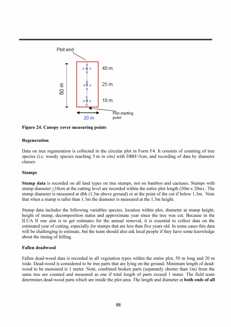
88

Figure 24. Canopy cover measuring points

Regeneration Data on tree regeneration is collected in the circular plot in Form F4. It consists of counting of tree species (i.e. woody species reaching 5 m in situ) with DBH<5cm, and recording of data by diameter classes. Stumps Stump data is recorded on all land types on tree stumps, not on bamboo and cactuses. Stumps with stump diameter >10cm at the cutting level are recorded within the entire plot length (50m x 20m).. The stump diameter is measured at dbh (1.3m above ground) or at the point of the cut if below 1.3m. Note that when a stump is taller than 1.3m the diameter is measured at the 1.3m height. Stump data includes the following variables species, location within plot, diameter at stump height, height of stump, decomposition status and approximate year since the tree was cut. Because in the ILUA II one aim is to get estimates for the annual removal, it is essential to collect data on the estimated year of cutting, especially for stumps that are less than five years old. In some cases this data will be challenging to estimate, but the team should also ask local people if they have some knowledge about the timing of felling. Fallen deadwood Fallen dead-wood data is recorded in all vegetation types within the entire plot, 50 m long and 20 m wide. Dead-wood is considered to be tree parts that are lying on the ground. Minimum length of dead-wood to be measured is 1 meter. Note, combined broken parts (separately shorter than 1m) from the same tree are counted and measured as one if total length of parts exceed 1 meter. The field team determines dead-wood parts which are inside the plot area. The length and diameter at both ends of all

89

pieces of fallen wood with diameter larger or equal to 10 cm within the plot area are measured. Standing dead trees are measured as normal tally trees. Data on fallen trees are registered in F6, and they consist of species, two diameter measurements, length and decomposition status. Thus, tree species of dead-wood should be detected when possible. Measurements of length are made to the plot border (Figure 25). Hence when a stem crosses the plot border, length and diameter are measured to/from that limit where the stem’s centre line crosses the border.

Figure 25. Selection of dead-wood parts in the plot

Two diameter measurements are carried out: the first measurement in the base part of the stem (or branch), the second in the other end (Figure 26). Use caliper to measure fallen dead-wood diameters. The diameters are measured over bark if bark exists. Record also if the measurement is done over or under bark. For measurements at the bases of fallen, buttressed trunks, diameters are measured above the buttress. The total length of the stem part larger than or equal to 10 cm in diameter is also recorded. If a part of laying stem has been removed from the plot (e.g. for making charcoal), the remaining main wood particles are recorded if they are larger than or equal to 10cm in diameter. If there are several

90

dead trees or dead-wood parts on the plot (as branches), then the recorder can tally the estimated mean dimensions of dead-wood and give the total number of stems/parts.

ote: Record this type of dead tree into two forms: Dead-wood data (Form 6, part B) and Stump data (Form 6, part A). Stump diameter is equal to Diameter 1 in the figure above. Diameter 2 cannot be less than 10 cm.

Figure 26. Dead-wood measurements

Decay class is detected applying two classes: solid wood or (partially) rotten wood. This can be detected by pushing a knife into the wood. Decay class is used when we compute dead-wood biomass and carbon: rotten coarse woody debris has a lower density value than solid wood. A dead laying stem can contain the stump part with some roots. In case of a broken dead tree the stump can be located in the plot. In both cases the stump data is recorded into the Stumps section on the field form 5, Part A. Bamboo Bamboo data is recorded in all vegetation types within a subplot 25m long and 20m wide.

a)

b) c)

91

Annex 3. Definitions

Abiotic: Pertaining to the non-living parts of an ecosystem, such as soil particles bedrock, air, and water. Afforestation: The establishment of a forest or stand in areas where the preceding vegetation or land use was not forest. Agroforestry: A collective name for land-use systems and practices in which trees and shrubs are deliberately integrated with non-woody crops and (or) animals on the same land area for ecological and economic purposes. Biotic factor: Any environmental influence of living organisms (e.g., damage by animals) in contrast to inanimate (i.e., abiotic) influences. Bole height: Bole height refers to merchantable height that is defined as the distance from the base of the tree to the first occurrence of the lowest point on the main stem, above the stump, where the stem form is changing or utilization of the stem is limited by branching or other defect. Breast height: Breast height is the height of 1.3 m from the ground level, or if the ground level cannot be defined, from the seeding point. See more explanations and special cases in the section Tree diameter measurements. Dead tree: A tree is regarded as dead tree if it does not have any living branches. Trees that are alive but so badly damaged that cannot grow in the next growing season (e.g. trees felled by storm) are regarded as dead trees. Dead-wood: Includes all non-living woody biomass not contained in the litter, either standing, lying on the ground, or in the soil. Dead-wood includes wood lying on the surface, dead roots, and stumps larger than or equal to 10 cm in diameter. Forked tree: If the forking point is below the breast height (1.3 m), each fork is recorded as a unique tree. If the forking point is above the breast height, a tree is recorded as one stem. Ground level: Ground level is described as in the following figure.

92

Living tree: A live tree must have living branches. The tree must be able to survive at least to the next growing season/next year. Permanent Sample Plot (PSP): PSPs will be periodically remeasured. They will provide data on changes in land use, forest stocking, volume and carbon. The locations of PSPs are measured using high-precision GPS. Sample tree: A live tree selected for measurements of additional parameters. Note: First tree of each tree species and every 5th tree in the plot are selected as sample trees. Seeding point: Seeding point is usually at the ground level. Trees that grow on the top of a stone or old stump, the seeding point is the point where the seeds have started to grow. Shrub: Shrubs are woody perennial plants, generally of more than 0.5 m and (usually) less than 5 m in height on maturity and with many stems and branches. Tally tree: Live or dead standing tree in the sample plot above minimum DBH. Tree: A tree is at least 1.35 m tall perennial woody plant with distinct stem capable of reaching 5 meters height in situ. Palms are regarded as trees in the data collecting phase, but distinguished in the data analysis phase. Bamboos, cactuses, lianas and shrubs are not recorded as trees. Ficus sp. are considered trees. Tree height: Tree height is the distance along the stem axis between the seeding (base) point and the tree tip. If the seeding point is higher than the ground level (e.g. in case where a tree growing on the top of a stone), the tree height is measured from the seeding point. See more explanations and special cases in the section Tree height measurements. Undergrowth: Undergrowth includes small trees, bushes, herbs and grasses growing beneath taller trees in the forest or other wooded land.

93

Annex 4. Slope Correction & Slope Correction Table

Slope Correction All reference distances, such as a tree distance from plot centre point, are expressed as horizontal distances. Thus, plot areas are also computed upon horizontal plane. When the terrain is flat, distances can be measured directly. But on sloping terrain the horizontal distances differ from direct (slope) distances (see Figure below). A corrected distance is taken from a slope correction table and these distances are applied at all slopes greater than or equal to 5 percent.

Figure 27. Distances on slope

+ote: The distance between two points, measured along slope (d1) is always longer than an equivalent horizontal distance (h1). On slope terrain, the horizontal distance must be multiplied by a factor that corresponds to the inclination, in order to obtain a corrected distance. Slope is measured using a Suunto hypsometer. The unit in this inventory is percent. Where distances are measured using a measuring tape on sloping ground, slope distance will need to be corrected back to horizontal using Slope Correction Table. Note: The points recorded by the GPS will reflect horizontal distance. No corrections for distances on slope are required.

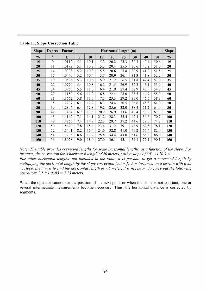
94

Table 11. Slope Correction Table

Slope Degree Factor Horizontal length (m) Slope

% o

fs 5 10 15 20 25 30 40 50 %

15 9 1.0112 5.1 10.1 15.2 20.2 25.3 30.3 40.4 50.6 15

20 11 1.0198 5.1 10.2 15.3 20.4 25.5 30.6 40.8 51.0 20

25 14 1.0308 5.2 10.3 15.5 20.6 25.8 30.9 41.2 51.5 25

30 17 1.0440 5.2 10.4 15.7 20.9 26.1 31.3 41.8 52.2 30

35 19 1.0595 5.3 10.6 15.9 21.2 26.5 31.8 42.4 53.0 35

40 22 1.0770 5.4 10.8 16.2 21.5 26.9 32.3 43.1 53.9 40

45 24 1.0966 5.5 11.0 16.4 21.9 27.4 32.9 43.9 54.8 45

50 27 1.1180 5.6 11.2 16.8 22.4 28.0 33.5 44.7 55.9 50

60 31 1.1662 5.8 11.7 17.5 23.3 29.2 35.0 46.6 58.3 60

70 35 1.2207 6.1 12.2 18.3 24.4 30.5 36.6 48.8 61.0 70

80 39 1.2806 6.4 12.8 19.2 25.6 32.0 38.4 51.2 64.0 80

90 42 1.3454 6.7 13.5 20.2 26.9 33.6 40.4 53.8 67.3 90

100 45 1.4142 7.1 14.1 21.2 28.3 35.4 42.4 56.6 70.7 100

110 48 1.4866 7.4 14.9 22.3 29.7 37.2 44.6 59.5 74.3 110

120 50 1.5620 7.8 15.6 23.4 31.2 39.1 46.9 62.5 78.1 120

130 52 1.6401 8.2 16.4 24.6 32.8 41.0 49.2 65.6 82.0 130

140 54 1.7205 8.6 17.2 25.8 34.4 43.0 51.6 68.8 86.0 140

150 56 1.8028 9.0 18.0 27.0 36.1 45.1 54.1 72.1 90.1 150

+ote: The table provides corrected lengths for some horizontal lengths, as a function of the slope. For instance, the correction for a horizontal length of 20 meters, with a slope of 30% is 20.9 m. For other horizontal lengths, not included in the table, it is possible to get a corrected length by multiplying the horizontal length by the slope correction factor fs. For instance, on a terrain with a 25 % slope, the aim is to find the horizontal length of 7.5 meter, it is necessary to carry out the following operation: 7.5 * 1.0308 = 7.73 meters. When the operator cannot see the position of the next point or when the slope is not constant, one or several intermediate measurements become necessary. Thus, the horizontal distance is corrected by segments.

95

Annex 5. Description of the 17 vegetation types in Zambia

Source: Zambian vegetation classification / mapping update – 2003

VEGETATIO/ TYPE DESCRIPTIO/ OF THE VEGETATIO/ TYPE

CLASS 1 (Dry Evergreen Forest) - This is a three-storey forest with closed evergreen or semi-deciduous canopy

25 to 27m high with occasional taller emergents, a discontinuous evergreen under storey 9 to 15m high and a

dense evergreen shrub-scrambler thicket 1.5 to 6m high. It occurs in three distinctive sites; (a) plateau, (b) the

bangweulu lake basin, and (c) northern Kalahari basin, always on level and gently undulating ground. The

disturbance of these forests by fire and cultivation results in degrade to Miombo woodland or Kalahari woodland,

or chipya. There are five sub forest classes that make up the dry evergreen forest namely;

Code: 01

Parinari Forest

Canopy dominants are restricted to Parinari excelsa and Syzygium guineense ssp,

Afromontanum with odd emergent Entandrophragma delevoyi, Marquesia

macroura and Erythlophleum suaveolens are occasional canopy associates. Partial

destruction of the Parinari forest results in a gradual regression to Miombo

woodland (or Copperbelt chipya) in which the forest overwood may have been

replaced by Brachystegia speciformis or Brachystegia microphylla. Complete

destruction of Parinari forest results in a Chipya identical with Lake basin chipya.

Code: 02

Marquesia Forest

Canopy dominants are restricted to Anisophyllea pomifera, Marquesia macroura,

Podocarpus milanjianus locally and Syzygium guineense spp, afromontanum.

Partial destruction of Marquesia forest results in a gradual regression to Miombo

woodland. Total destruction results in Lake basin chipya.

Code: 03

Lake Basin Chipya

This is three-storey woodland with an open evergreen to deciduous canopy 21 to

27m high characterized by Albizia antunesiana, Burkea Africana, Combretum

collinum, Erythlophleum africanum, Parinari curatellifolia, Pericorpsis

angolensis, Pterocarpus angolensis and Terminalia sericea. Bracken Aframomum

and Smilax are characteristic of the forest floor. This type may occur on isolated

patches of lake basin type soil well separated from the true Lake Basin.

Code: 04

Cryptosepalum Forest

Canopy dominant are restricted to Cryptosepalum exfoliatum spp, Pseudotaxus and

Guibourtia coleosperma in the lower rainfall areas of Zambezi, Kabompo and

Kaoma districts but associated with Marquesia acuminate, Marquesia macroura,

Parinari excelsa and Syzygium guineense ssp, afromontanum in the high rainfall

areas of Mwinilunga district. Partial destruction of cryptosepalum forest leads to

miombo / kalahari woodland, but total destruction leads to kalahari sand chipya.

Code: 05

Kalahari Sand Chipya

Kalahari sand chipya’s canopy is characterised with Burkea Africana, Combretum

collinum, Dialium engleranum, Erythrophleum africanum, Guibourtia

coleosperma, Peltophorum africanum, Pterocarpus angolensis and Terminalia

sericea and there is a dense growth of aframomum and bracken on the forest floor.

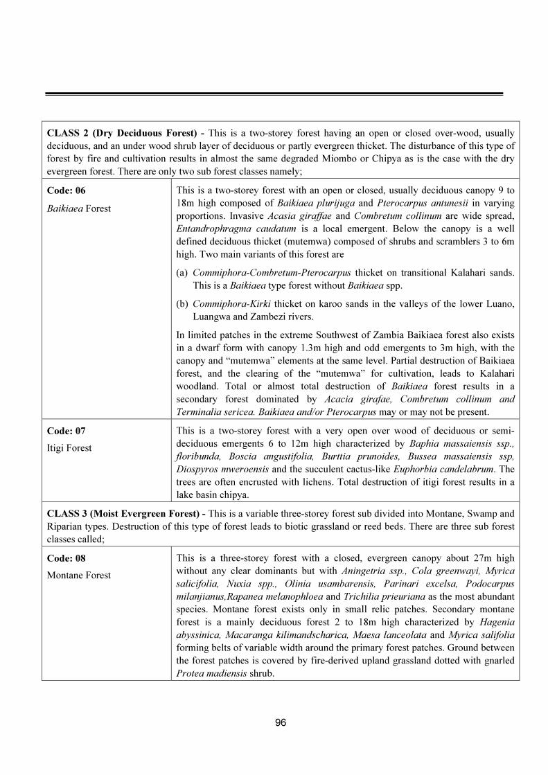
96

CLASS 2 (Dry Deciduous Forest) - This is a two-storey forest having an open or closed over-wood, usually

deciduous, and an under wood shrub layer of deciduous or partly evergreen thicket. The disturbance of this type of

forest by fire and cultivation results in almost the same degraded Miombo or Chipya as is the case with the dry

evergreen forest. There are only two sub forest classes namely;

Code: 06

Baikiaea Forest

This is a two-storey forest with an open or closed, usually deciduous canopy 9 to

18m high composed of Baikiaea plurijuga and Pterocarpus antunesii in varying

proportions. Invasive Acasia giraffae and Combretum collinum are wide spread,

Entandrophragma caudatum is a local emergent. Below the canopy is a well

defined deciduous thicket (mutemwa) composed of shrubs and scramblers 3 to 6m

high. Two main variants of this forest are

(a) Commiphora-Combretum-Pterocarpus thicket on transitional Kalahari sands.

This is a Baikiaea type forest without Baikiaea spp.

(b) Commiphora-Kirki thicket on karoo sands in the valleys of the lower Luano,

Luangwa and Zambezi rivers.

In limited patches in the extreme Southwest of Zambia Baikiaea forest also exists

in a dwarf form with canopy 1.3m high and odd emergents to 3m high, with the

canopy and “mutemwa” elements at the same level. Partial destruction of Baikiaea

forest, and the clearing of the “mutemwa” for cultivation, leads to Kalahari

woodland. Total or almost total destruction of Baikiaea forest results in a

secondary forest dominated by Acacia girafae, Combretum collinum and

Terminalia sericea. Baikiaea and/or Pterocarpus may or may not be present.

Code: 07

Itigi Forest

This is a two-storey forest with a very open over wood of deciduous or semi-

deciduous emergents 6 to 12m high characterized by Baphia massaiensis ssp.,

floribunda, Boscia angustifolia, Burttia prunoides, Bussea massaiensis ssp,

Diospyros mweroensis and the succulent cactus-like Euphorbia candelabrum. The

trees are often encrusted with lichens. Total destruction of itigi forest results in a

lake basin chipya.

CLASS 3 (Moist Evergreen Forest) - This is a variable three-storey forest sub divided into Montane, Swamp and

Riparian types. Destruction of this type of forest leads to biotic grassland or reed beds. There are three sub forest

classes called;

Code: 08

Montane Forest

This is a three-storey forest with a closed, evergreen canopy about 27m high

without any clear dominants but with Aningetria ssp., Cola greenwayi, Myrica

salicifolia, .uxia spp., Olinia usambarensis, Parinari excelsa, Podocarpus

milanjianus,Rapanea melanophloea and Trichilia prieuriana as the most abundant

species. Montane forest exists only in small relic patches. Secondary montane

forest is a mainly deciduous forest 2 to 18m high characterized by Hagenia

abyssinica, Macaranga kilimandscharica, Maesa lanceolata and Myrica salifolia

forming belts of variable width around the primary forest patches. Ground between

the forest patches is covered by fire-derived upland grassland dotted with gnarled

Protea madiensis shrub.

97

Code: 09

Swamp Forest

This is a three-storey forest with a closed evergreen canopy to 27m. Common

species include Ficus capensis, Homalium africanum, Rauvolfia caffra, Ilex mitis,

Mitragyna stipulosa, Syzygium cordatum, S. owariense, Xylopia aethiopica, X.

rubescens and Uapaca guineense. Swamp forest occurs in high rainfall areas of

the country associated with the major catchment zones found in Zambia. These

areas are characterized by super abundance of ground water all year round. The

soil types mainly alluvials control moisture regimes and discharge of water into

lakes and rivers. It occurs in three forms: (a) estuarine swamp flooded all year

round; (b) seepage swamp with water table at or just above ground level all year

round; and (c) seasonal swamp flooded during the rainy season and with the water

table near ground level for the rest of the year.

Code: 10

Riparian Forest

This is a three-storey forest with a closed evergreen canopy to 25m high

characterized by Diospyros mespiliformis, Khaya nyasica Parinari excelsa and

Syzyfgium cordatum, associated with Adina microcephala, Bridelia micrantha,

Cleistanthus milleri, Faurea saligna, Homalium africanum, Ilex mitis, Manilkara

obovata and Raphia palms. The composition varies from a northern veregeen

element and southern deciduous element. Most riparian forest in the territory is

wholly or partially secondary. Characteristic secondary species include Acasia

polyancantha, Salix subserrata, Terminalia sericea and Zizphus spp. Climbers are

frequent.

CLASS 4 (Woodlands) - This has a one-storey (sometimes two-storey) structure with a dense ground cover of

suffrutices and grasses. The Miombo woodland is probably derived from degraded types 1 and 2, the Kalahari

woodland from degraded type 4 and 6

Code: 11

Miombo Woodland

This is two-storeyed woodland with an open or partially closed canopy of semi-

evergreen trees 15 to 21m high characterized by species of Brachystegia,

Isoberlinia, Jubernardia and Marquesia macraura with Erythrophleum africanum,

Parinari curatellifolia and Pericopsis angolensis as frequent associates. The forest

floor is covered by a more or less dense grass cover. Relic patches of evergreen

thicket may or may not be present. Most Miombo woodland is secondary re-

growth as a result of extensive cultivation in the past. The Miombo woodland also

spreads from the plateau onto the adjacent hills and down the escarpments, and

also occurs as a relic in the major river valleys. In the west it has invaded the

Kalahari sands to become Miombo/Kalahari woodland which extends beyond the

border of Zambia.

Code: 12

Hill Woodland

Where there are more rocks than sand on the hills, the Brachystegias and their

allies almost die out except for Brachystegia microphylla, and Brachystegia

glaucescens and their place is taken by characteristic hill shrubs such as

Aeschynomene rubrofarinacea and Aeschynomene semilunari, Euphorbia

ussanguensis and Euphorbia griseola, Myrothanmnus flabellifolius, Pentas

nobilis, Vellozia equisetodes and Vellozia tomentosa, and Vernonia bellinghamii.

Code: 13

Kalahari Woodland

This is a two-storey woodland with an open or partially closed, deciduous or semi-

deciduous over wood 18 to 24m high characterized by Ambloygonocarpus

98

andongensis, Burkea Africana, Combretum collinum, Cryptosepalum exfoliatum

ssp. Pseudotaxus, Dialium engleranum, Erythlophleum africanum, Guibortia

coleosperma, Parinari curatellifolia and Terminalia sericea. The Kalahari

woodland embraces all woodlands on kalahari sands. The vegetation is derived

from the partial destruction of dry deciduous Baikiaea forest. It forms a catenary

regression from Baikiaea forest to suffrutex savanna to grassland on kalahari

sands. Five stages are distinct in composition namely Guibourtia woodland,

Burkea erythrophleum woodland, Burkea-Diplorhynchus scrub, Diplorhynchus

scrub and Parinari suffrutex savanna.

Code: 14

Mopane Woodland

This is a one-storeyed woodlands with an open deciduous canopy 6 to 18m high.

The dominant colophospermum mopane is pure or almost pure. Scattered

elemements of munga woodland occur here and there represnted chifly by acacia

nigrescens, adansonia digitata, combretrum imberde , kirkia acuminate and

lannea stuhlmannii. The python vine fockea multiflora, is usually present .

Mopane-munga ecotones are more common then pure mopane woodland . two

extreme variant can be recognised; a rich variant on sandland or mudstone above

and an impoverished variant on sandstone or mudstone as abave and an

impoverished variant on akeletal mudstone or pebble beds . the latter is a low open

scrub of colophospermum mopane, terminalia randii and/ or t. stuhlmannii

Code: 15

Munga Woodland

This is a coined term for savanna woodland .it is an open, park-like, 1 to 2 storeyed

deciduous woodland with scattered or grouped emergents to 18m high

characterised particularly by acacia, combretum and ter minalia species.

occasionally it has a deciduous or semi-deciduous thcket understorey. mungu

woodland is divided into; [a] upper valley sites mainly in central province [b]

lower valley in the luangwa and mid Zambezi valley, and [c] Kalahari sites on the

Kalahari sands. On the first two sites there tends to be a combretum-terminalia

variant on the more elevated, better-drained sites and an acacia variant on the

lower, poorer drained sites.

The penultimate stage in the degradation of munga woodland is what is usually

referred to as dambo-margin vegetation which is wide so spread throughout the

territory.

CLASS 5 (Other Vegetation Types) - All types of vegetation, i.e. forest, woodland, thicket, scrub and grassland

can be found on or around the bases of termitaria. They have been classified by habitat rather than by vegetation

type, because to some extent one limits the other.

Code: 21

Termitaria Vegetation

and bush groups

(a) Miombo termitaria are characterised by Albizia camara, Boscia angustifolia,

Cassine aethiopica, Combretum molle, Commiphora mollis, Erythrina

abssynica, Euphorbia candelabrum and Ziziphus mucronata in their upper

storey.

(b) Kalahari termitaria are characterised by Boscia albitrunca, Combretum

imberbe, Diospyros mespiliformis and Strychnos potatorum

(c) Mopane termitaria are characterised by Acasia nigrescens, Albizia harveyi,

99

Colophospermum mopane, Garcinia livingstonei, Kirkia acuminate, Lannea

stuhlmannii and Markhamia acuminate.

(d) Munga termitaria are characterised by Albizia harveyi, Combretum imberbe,

Lannea stuhlmannii, Manilkara mochisia and Strychnos potatorium.

(e) Riparian termitaria are characterised by Apodytes dimidiate, Erythrophleum

sauveolens, Garcinia livingstonei, Parinari curatellifolia and Syzygium

cordatum.

(f) Some bush groups (e.g. in Chinsali and Kaoma Districts) are based on

termitaria along the margins of seepage dambo and flood plain. Other bush

groups (e.g. in Senanga District) are not based on termitaria but are isolated

patches of Type 13 on slight elevations surrounded by grassland.

Code: 31 and 32

Grasslands

The grasslands are edaphic grasslands associated with the drainage lines. They can

be divided into dambo (headwater valley) grassland, river-line grassland and

floodplain grassland. These are associated with the streams and rivers; floodplains

of the larger rivers like the Zambezi, Luapula, Kafue and Chambeshi; Seasonally

flooded fresh water swamps like Bangweulu; Lukanga; Busanga and Mweru

Wantipa; and some alkaline swamps which evaporate to salt. Mountain grassland

and watershed plains are also included.

/OTE – For a more detailed account of the vegetation types read Forest Research Bulletin No. 7: “Vegetation of

Zambia” Printed by the Government Printer, Lusaka, 1971.

100

Annex 6. Relocating the old Marker (ILUA I Plot)

Triangulation method is used to find out the old markers on ILUA I plots. When the marker was installed during ILUA I, at least three references were recorded. These references are registered on the field form one (FF1) of the each tract. The references of the marker (installed in the first plot in Tract 31) are registered as follow: 44. ID 45. Description 46. Bearing ˚ 47. Distance in m 36. Photo ID

1 Northern edge of the rock 280˚ 26 031.1.1 2 East edge of the anthill 51˚ 19 031.1.2 3 Baobab tree 108˚ 26 031.1.3

To relocate the old marker, the following steps can be taken: - Collect the information about references and marker in the previous reports and field forms (ILUA I); - Save the Marker position coordinates in the GPS receiver; - Navigate to the marker location using the GPS; - Stop when you arrive at the marker location; - Try to find the marker first. - But if the marker is not found look for references; - From the identified and relocated reference point, take the bearing; - Measure the distance to the suspected marker location and draw an arc; - Repeat the three last steps for the second and third reference objects; - Clean the suspected area; - If you do not find the marker, use the metal detector to find the Marker. The next figure describes the triangulation method.

R

1

R

3

Bearing

R

2

Back Bearing 100

M

�

Figure 28. Triangulation method

101

Annex 7. Use of Disc Pasture Meter for grass measurement

The Disc Pasture Meter (DPM) is an instrument that measures herbaceous biomass, but more specifically, the

grass component.

A. How does it work? - Usually one would measure herbaceous biomass through clipping, drying and

weighing. You use a manageable quadrat size of say 0.5 m2 and you clip all the plants in it to ground

level. Place in a bag, take back to the lab, oven dry it and weigh it. This can be a time consuming

process. This is why the DPM was developed. The instrument is basically an aluminum disc that you

drop from a standard height and the height it settles at is related to the density of the grass and/or herb

layer. In theory, the denser and taller the layer, the higher the DPM will settle at.

The DPM consists of three parts (Figure 29): 1) aluminum measuring stick, 2) handle and 3) disc. It has

a stopper on the measuring rod which prevents you from lifting the disc higher than the constant height.

Figure 29. Disc Pasture Meter

B. How to take a reading? - The DPM works on the principle that the taller and denser the grass is the

higher the disc will settle on the grass layer (Figure 30). Take a reading is as follows: place the

measuring rod on a random point, lift the disk by the handle until it reaches the stopper and simply let it

go. However, placing the plate gently on the forage is more satisfactory than dropping the plate

especially on hills or on windy days.

The disk will settle on the grass. Read the height at from the measuring stick, record it and the grass

species.

In short, sparse grass the DPM settles lower than in tall, dense grass. When selecting the sample

location the user should be careful not to bias the average by choosing more productive areas over less

productive areas.

102

Figure 30. Use of Disc Pasture Meter

C. Calibrating the DPM - The DPM needs to be calibrated for specific regions by clipping and weighing

grass samples and reading the heights. Calibration is done by selecting a fairly large quadrant, 10 m2.

Measure the area accurately. In this quadrant take 8-10 DPM readings. Next comes the hard part: you

have to clear cut the entire quadrant, dry all the material and weigh it.

Compute the average of your DPM readings and from the weigh the collected samples, and compute the

average biomass per square meter. Also identify the grass species in the quadrant and rank them

according to abundance. This will help you to calculate the proportion of each species of the total grass

biomass. Repeat this procedure across vegetation types in order to capture the range of grass densities

and heights. Ultimately you can reduce the error of the DPM measurements by taking many

measurements over a large area.

D. One additional measurement - While doing a DPM survey, one quick additional measurement can add

a lot of value to your dataset. That is point to tuft distance - at the point where you have stopped to take

the DPM reading, estimate also the distance from the tip of your shoe to the nearest grass tuft. You can

estimate it, and if you are standing on a tuft the distance is 0, or one hand breadth is 10 cm, and so on,

and if it is bare land for next 1 m (or more) then the DPM record is a miss or just null (on bare land).

103

Annex 8. ILUA II protocol for plant collection and processing

This procedure has been compiled based on practice as adapted from the collection guidelines illustrated by the Kew herbarium manual. It presents the standard practice of collection procedure of plant specimens for determination. It illustrates what to do with plants that cannot be identified in the field. a. Equipment In the preparation and execution of inventories and botanical collection work, the following equipment should be mobilized;

o Secateurs and scissors for trimming specimens o Double flimsy or newspaper (specimen folder) for retaining plant through out the process o Drying, bloating or absorbent paper as a sacking material o Press frames which should slightly be bigger than flimsies, newspaper or drying paper o Press straps for holding the press, applying and maintaining pressure o Aluminum corrugated sheets for increasing ventilation o Paper strips for securing o Paper and mesh bags for collecting carpological materials o Polythene bags big enough to contain whole bundles of dry or spirit specimens

b. Collection process 1) Any plant that is not identified to species level must be collected for herbarium voucher 2) The valid voucher must meet standard herbarium requirements

a. Using a secateurs cut a sample part of plant material b. As a rule of the thumb all specimens must be valid specimens c. Invalid specimens should be avoided as they are irrelevant for determination d. Specimen must represent the carious traits and characters of the plant e. Both sides of the floral members must be sufficiently represented and exposed f. The specimen should carry the description and collectors identification details showing :-

i. Collectors identification details which is coded by initials of lead collectors and members of the collection team

ii. Specimen collectors number which should start with 01 or continue from the last collection number if the collector has been involved in collection before

iii. Description of features that change form such as colour, scent, frequency and others)

iv. See appended note 1 for order of specimen description g. All collected materials should be processed for pressing using standard pressing procedures

i. It is preferred to make quick arranged processing overnight and carry out fine adjustments in the evening or the following morning

ii. If leaves are crowded some of them should be removed but at least the petioles should be left attached to show position of the leaves

iii. Cut stems and branchlets obliquely to show internal structure iv. Large leaves can either be trimmed on one side of the midrib and folded or cut

into sections

104

v. Each single specimen must be placed in either flimsy paper or newspaper vi. Each specimen must be separated by bloating paper, which must be changed every

new day until the specimen are sufficient dry (average 3 days) vii. Specimens must be dried in a press viii. Specimens must separated by aluminum gauzes for every 15 to 20 sets of

collection ix. Place the prepared specimens should be kept in the open with good ventilation for

to support drying x. Once dried the materials must be kept dry during the entire period in the field xi. Materials must be securely packed for final transit and kept dry

c. Additional notes

- Specimens with thick or humpy parts, folds of drying paper may be added for support or as padding to the more delicate structures to help distribute the pressure

- Insufficient or uneven distributed pressure may cause wrinkle to the specimens - Stems and roots can be cut lengthwise and projecting braches trimmed off - Each press should be examined regularly for tightness and turned so that the drying is even - The collection number should be written on a number tag attached to the specimen in addition

to the folder - It is especially important to add numbers sequentially for collected parts of a large plant - Specimens should stay in folder until the ultimate destination is reached

CODIG SYSTEM The coding system for a collected valid specimen will be: - ILUAII/Initials of all collectors/specimen # For database, code numbering will need to reflect cluster ID and lead collector only as: ILUAII/Cluster ID/Initials of lead collector/Specimen # 1. SEE EXAMPLE BELOW: (FOR NEW COLLECTOR) Lead Collector: Keddy M. Mbindo (KMM) Other members in the collection team: Noah B. Zimba (NBZ), Mokwani Kaluwe (MK), The first valid specimen collected by lead collector Keddy M.Mbindo and team will be numbered as below unless the collector has an already running collection number series which he/she should continue on:- ILUAII/KMM, BZ, MK 01 For database the corresponding code numbers that will be entered for the above specimen will also contain cluster ID but only capture initials of lead collector as:- ILUAII/Cluster ID/KMM/01

105

Second specimen by same collector will be ILUAII/KMM, BZ, MK 02 For database the code number for the specimen will be ILUAII/Cluster ID/KMM/02 2. EXAMPLE FOR COLLECTOR WITH ALREADY RUNNING NUMBER SERIES Lead Collector: Noah B Zimba (e.g. whose last series number for collections is 3101) Other members in collection team: Keddy M. Mbindo, Mokwani Kaluwe, Bwalya Chenduaka First specimen collected by collector will be coded as below: ILUAII/BZ, KMM, MK, BC 3102 For database the code number for the specimen will be ILUAII/Cluster ID/BZ/3102 To keep track of specimen all the collectors have to have their own permanent collectors book and it cannot be shared. Each collector has to submit the book together with the specimens.

106

Annex 9. Field soil texture and structure assessment

Soil texture

Soil texture refers to the proportion of the various particle-size classes (or soil separates, or fractions) in a given

soil volume and is described as soil textural class. The names for the particle-size classes correspond closely

with commonly used standard terminology. The textural class can be estimated in the field by simple field tests

and feeling the constituents of the soil (Hand Feel Flow Chart Method –see Figure 31); take a well-mixed soil

sample 2- 3 table spoon size in the hand. The soil sample must be in a moist to weak wet state with water.

Gravel and other constituents >2mm must be removed. The constituents have the following feel: Clay: soils

fingers, is cohesive (sticky), is formable, has a high plasticity and has a shiny surface after squeezing between

fingers, Silt: soils fingers, is non-sticky, only weakly formable, has a rough and ripped surface after squeezing

between fingers and feels very floury (like talcum powder), and Sand: cannot be formed, does not soil fingers

and feels very grainy.

Figure 31. Assessment of Soil Texture in the Field

Source: Woode, 1988

Soil structure

Soil structure refers to the natural organization of soil particles into discrete soil units (aggregates or peds) that

result from pedogenic processes. The aggregates are separated from each other by pores or voids (Figure 32). It

107

is preferred to describe the structure when the soil is dry or slightly moist. In moist or wet conditions, it is

advisable to leave the description of structure to a later time when the soil has dried out. For the description of

soil structure, a large lump of the soil should be taken from the profile, from various parts of the horizon if

necessary, rather than observing the soil structure in situ. Soil structure is described in terms of grade, size and

type of aggregates. Where a soil horizon contains aggregates of more than one grade, size or type, the different

kinds of aggregates should be described separately and their relationship indicated.

Figure 32. Assessment of Soil Structure

Source: FAO, 2006

108

References

British Columbia Ministry of Forests. 2008. Glossary of Forestry Terms in British Columbia. Province of British Columbia, Canada. Available at: http://www.for.gov.bc.ca/hfd/library/documents/glossary/ Chidumayo E. 2012a. Assessment of existing models for biomass and volume calculations for Zambia. Report prepared for Integrated Land Use Assessment phase II. Chidumayo E. 2012b. Classification of Zambian forest. Report prepared for Integrated Land Use Assessment phase II. FAO. 2007. Global Forest Resources Assessment 2010 – Specification of +ational Reporting Tables for FRA 2010. FRA Working Paper No 135. Rome. 51 p. FAO. 2008. Technical Review of FAO’s Approach and Methods for +ational Forest Monitoring and Assessment (+FMA). By Erkki Tomppo and Krister Andersson. National Forest Monitoring and Assessment Working Paper NFMA 38. Rome FAO. 2009. +ational Forest Monitoring and Assessment – Manual for integrated field data collection. Version 2.3. National Forest Monitoring and Assessment Working Paper NFMA 37/E. Rome. FAO. 2010a. National forest resources monitoring and assessment of Tanzania (NAFORMA), Field Manual – Biophysical survey (M01-2010). Forestry and Beekeeping Division, Ministry of Natural Resources and Tourism Forestry and Beekeeping Division. FAO. 2010b. National forest resources monitoring and assessment of Tanzania (NAFORMA), Field Manual – Socioeconomic survey (M05-2010). Forestry and Beekeeping Division, Ministry of Natural Resources and Tourism Forestry and Beekeeping Division. FSP 2003. Zambia Forest Resource Assessment 2003. EU – Forestry Support Programme in Zambia – 8 ACP/ 051. Holechek J. & Galt D. 2000. Grazing intensity guidelines. Rangeland 22(3):11–14. IPCC 2008. 2006 IPCC Guidelines for +ational Greenhouse Gas Inventories – A primer. Prepared by the National Greenhouse Gas Inventories Programme, Eggleston H.S., Miwa K., Srivastava N. and Tanabe K. (eds). Publisher: IGES, Japan. Kalinda T., Bwalya S., Mulolwa A. & Haantuba H. 2008. Use of Integrated Land Use Assessment (ILUA) data for forestry and agriculture policy review and analysis in Zambia (FAO – Forestry Department) Lungo C. 2012. Biophysical information needs assessment report (draft). Report prepared for Integrated Land Use Assessment phase II.

109

METLA 2006. VMI10 Maastotyöohje. Field Manual for NFI-10 in Finland. Finnish Forest Research Institute. Helsinki, Finland. (in Finnish). Mfune O. 2012. Forest governance monitoring information gaps (draft). Report prepared for Integrated Land Use Assessment phase II. Michalak R. 2008. Comparison of the scope, terms, definitions and classifications applied for the FAO Global Forest Resources Assessment 2010 and the MCPFE/U+ECE/FAO Report on State of Europe’s Forests 2007. Part I - Definitions and classifications structured according to FRA reporting tables. UNECE/FAO Timber Section, Geneva. 38 p. Mukosha J., Siampale A. 2008. Integrated Land Use Assessment 2005-2008 report. Zambia Forestry Department/MTENR and FAO. 147 p. Neyman, J. 1938. Contribution to the theory of sampling from human populations. J. Am. Statist. Ass., 33. Pp. 101-116. Storrs, A. E. G. 1979. Know your trees - some of the common trees found in Zambia. Forestry Department, Ndola. 380 p. Tomppo E. & Tavani R. 2012. Exploratory sampling study in preparation for the FAO supported second phase of the National Integrated Land Use Assessment (ILUA2) in Zambia. Report paper. Woodall C.W., Rondeux J., Verkerk P.J. & Ståhl G. 2006. Estimating Dead Wood During +ational Forest Inventories: A Review of Inventory. Methodologies and Suggestions for Harmonization. Proceedings of the Eighth Annual Forest Inventory and Analysis Symposium.