zhang li dong lic
DESCRIPTION
ZhangTRANSCRIPT

Abstract
A voltage dip is a reduction in the voltage magnitude with a durationbetween a few cycles and several seconds. Voltage dips are consideredone of the most serious power quality problems. They lead to mal-operation or tripping of several types of end-user equipment, e.g.adjustable speed drives, computers, etc. A dip is often characterized byone magnitude and one duration. This is a reasonable approximation aslong as single-phase equipment (e.g. computers) are concerned.However, three-phase equipment (e.g. adjustable-speed drives) willtypically experience three different voltage magnitudes, as the majorityof dips are due to single-phase or phase-to-phase faults. The three-phase voltage relation of the power supply during a dip needs to beanalyzed to assess the influence of voltage dips on three-phaseequipment.
The three-phase unbalance of voltage dips in their characterization andpropagation is dealt with in this dissertation. A dip classificationmethod is proposed. The classification method is applied to analysevoltage dip measurement from power quality survey, and to test three-phase equipment immunity against voltage dips.
The dip classification is based on the well-proven theory ofsymmetrical components. Mathematical models are developed for bothbalanced and unbalanced dips, taking into account the fault types,transformer types and load connections. The characterization results ina so-called characteristic voltage (a generalized magnitude and phase-angle shift) for balanced and unbalanced dips as well as a so-calledPN-factor, relating to the dynamic loads contribution to the sourceimpedance for unbalanced dips. The PN-factor is equal to unity if thepositive- and negative-sequence source impedance of the system areequal and time-independent. With several acceptable assumptions, theclassification method is able to quantify all three-phase dips by onesingle complex number, namely the characteristic voltage. Thissignificantly simplifies the study of unbalanced dip propagation inpower systems. Field measurements show that the proposedclassification method holds for both transmission systems anddistribution systems. Theoretically, large dynamic loads connected tothe system could affect the correctness of the proposed method.However, the field measurements show that the error introduced bydynamic loads is negligible.

The proposed classification method helps understanding the phaserelationships of unbalanced voltage dips. The phase-angle shiftphenomenon associated with voltage dips is well explained by themathematical models introduced. In presenting voltage dipmeasurement from power quality survey and performing three-phaseequipment immunity test, the classification method offers a platform toexchange information between utilities, customers, and equipmentmanufacturers.
Keywords:
power systems, power quality, voltage dips(sags),symmetrical components, characterization, field measurement,equipment immunity test.

Preface
The work presented in this thesis has been carried out at theDepartment of Electric Power Engineering at Chalmers University ofTechnology. The research has been funded through the Elforsk Elektraprogram which is jointly financed by the Swedish National Board forIndustrial and Technical Development (NUTEK) and ABB CorporateResearch. The financial support is gratefully acknowledged.
I wish to express my deepest gratitude to my supervisor, Dr. MathBollen, for supervising this work, for valuable comments, fruitfuldiscussions and for persistently revising the manuscript. I also wouldlike to thank my examiner, professor Jaap Daalder, for his assistancethroughout this project and many helpful comments. Many thanks toall the colleagues at the department of Electric Power Engineering,especially to the power system group for general assistance in differentways.
Members of the steering group have been Ulf Grape, Mats Häger, andGunnar Ridell. Thank you all for fruitful discussions and valuablecomments.
Special thanks should also be given to Mats Häger of STRI, AlastairFerguson of Scottish Power, and Helge Seljeseth of SINTEF EnergyResearch for kindly offer of the field measurement data.
Last but not least, I would like to thank my wife Yibin for love andsupport, and for patiently waiting for a husband who often come backlate from work.
LIST OF PUBLICATIONS
This thesis is based on work reported in the following papers, referredto by Roman numerals in the text:
I L.D.Zhang, M.H.J. Bollen, A method for characterizing unbalancedvoltage dips (sags) with symmetrical components, IEEE PowerEngineering Letters, pp. 50-52, July 1998.
II L.D. Zhang, M.H.J. Bollen, Characteristics of voltage dips(sags) in powersystems, accepted by IEEE PES Transactions.
III L.D. Zhang, M.H.J. Bollen, A method for characterization of three-phaseunbalanced dips from recorded voltage waveshapes, InternationalTelecommunication Energy Conference(INTELEC), Copenhagen,Denmark, June 1999.
IV M.H.J. Bollen, L.D. Zhang, Analysis of voltage tolerance of ac adjustable-speed drives for three-phase balanced and unbalanced sags, accepted byIEEE Transactions on Industry Applications.
V M.H.J. Bollen, J. Svensson, L.D. Zhang, Testing of grid-connected powerconverters for the effects of short circuits in the grid, European PowerElectronics Conference, Lausanne, Switzerland, September 1999.

Contents
Abstract Preface ContentsChapter 1 Introduction 1
1.1 Voltage dips and related studies ...................................................... 11.2 Problem of three-phase unbalance ................................................... 31.3 Aim and layout of the thesis ............................................................ 4
Chapter 2 Terminology 7
2.1 Voltage dips and other voltage variations ........................................ 72.2 Voltage dips in one phase ................................................................ 92.3 Example of single-phase dip characterization ................................. 11
Chapter 3 Classification of Three-phase Voltage Dips 15
3.1 Balanced faults ................................................................................. 153.2 Unbalanced faults ............................................................................ 17
3.2.1 Two-component symmetrical components .......................... 173.2.2 Unbalanced faults analysis by sequence networks .............. 20
3.3 Definition of dip types ..................................................................... 223.3.1 The single-line-to-ground fault (SLGF) .............................. 223.3.2 The line-to-line fault (LLF) ................................................. 243.3.3 The double-line-to-ground fault (2LGF) ............................. 253.3.4 The three-phase fault (3ØF) ................................................. 253.3.5 Overview of the classification ............................................. 273.3.6 Phase-angle shift in unbalanced dips ................................... 283.3.7 Symmetrical phase for unbalanced dips .............................. 29
3.4 Dip transformation through transformers ........................................ 333.4.1 Basic transformer models .................................................... 343.4.2 Effect of the basic transformer models on the basic dip types 363.4.3 Change of the symmetrical phase ........................................ 383.4.4 Physical transformers to mathematic models ...................... 40
3.5 Terminology: three-phase voltage dips ............................................ 46
Chapter 4 Voltage Dip Propagation in Power Systems 47
4.1 Voltage dip propagation in distribution systems ............................. 484.1.1 Voltage dip propagates upwards and downwards ................ 504.1.2 SLGF at medium voltage level ............................................ 544.1.3 Local generation .................................................................. 55
4.2 Voltage dip propagation in transmission systems ........................... 564.3 A single-phase scheme to study voltage dip propagation ................ 60
4.3.1 Characteristic voltage .......................................................... 604.3.2 PN-factor .............................................................................. 624.3.3 Dip type ............................................................................... 64
4.4 Load’s influence .............................................................................. 644.4.1 Motor re-acceleration ........................................................... 654.4.2 PN-factor .............................................................................. 664.4.3 Limitations of the classification method .............................. 73
Chapter 5 Field Measurement Analysis 75
5.1 Obtaining dip characteristics ........................................................... 755.1.1 Principle ............................................................................... 75

Contents
5.1.2 Algorithms for dip characterization .....................................785.1.3 Examples ..............................................................................79
5.2 Characteristics obtained from measurements ...................................845.2.1 Transmission system: Sweden .............................................845.2.2 Distribution system: Scotland ..............................................865.2.3 Distribution system: Norway ...............................................87
5.3 Further application examples ...........................................................905.3.1 A propagating dip .................................................................905.3.2 Statistics from a power quality survey .................................94
Chapter 6 Equipment Immunity Tests 99
6.1 Single-phase equipment test .............................................................1006.1.1 Test items .............................................................................1006.1.2 Test setup .............................................................................1056.1.3 Test example ........................................................................109
6.2 Three-phase equipment test ..............................................................1116.2.1 Test items .............................................................................1126.2.2 Test setup .............................................................................117
Chapter 7 Conclusions and Future Research 119
7.1 Conclusions ......................................................................................1197.2 Future Research ................................................................................122
References 125App.A Determination of Zero-sequence Source Impedance 131App.B PN-factor and Characteristic Voltage 133
B.1 Single-line-to-ground Fault (SLGF) ...............................................133 B.2 Line-to-line fault (LLF) ..................................................................135

Chapter 1: Introduction
1
Chapter 1 Introduction
1.1 Voltage dips and related studies
Voltage dips are short duration reductions in rms voltage, mainlycaused by short circuits and starting of large motors. Disruptive voltagedips are mainly caused by short-circuit faults. Fault conditions onpower systems are the result of a variety of conditions, such aslightning, wind, equipment failure, accidents, etc. The large interest involtage dips is due to the problems they cause on several types ofequipment [1]. Specially computers, adjustable-speed drives andprocess-control equipment are notorious for their sensitivity.Equipment used in modern industrial plants (process controllers,programmable logic controllers, adjustable speed drives) is actuallybecoming more sensitive to voltage dips as the complexity of theequipment increases and the equipment is interconnected insophisticated processes. Voltage dips and short interruptions are themost troublesome and costly type of power quality problem for mostcustomers. Interruptions occur when a protective device actuallyinterrupts the circuit serving a particular customer. This will normallyonly occur when there is a fault on that circuit. Voltage dips occurduring faults in a wide part of the power system. Compared tointerruptions, voltage dips occur much more frequent. If equipment issensitive to these dips, the frequency of problems will be much higherthan if the equipment would be only sensitive to interruptions [2].
Over the last ten years, voltage dips have become one of the maintopics concerning power quality among utilities, customers andequipment manufacturers. Several international standards and workinggroup documents have been produced to improve the understanding ofvoltage dip problems[9][17][22][23].
Voltage dip related studies can be divided into the following categories:
1. Characterization of voltage dips
. These studies aim at acquiring aknowledge of the voltage dip characteristics[20][49][51]. Both faultpropagation studies and measured data are being used for this. Thereduction in rms voltage and the duration of event are the maincharacteristics. A voltage dip is normally characterized by onemagnitude and one duration [9][40][48]. However, several studies haveshown that some other characteristics associated with dips, such as

Chapter 1: Introduction
2
phase-angle shift, point-on-wave of initiation and recovery, waveformdistortion, and phase unbalance, may also cause problems for sensitiveequipment. These non-energy related characteristics receivedconsiderable attention in recent years [7][14][15][54].
2. Equipment immunity
. The equipment’s sensitivity is a major partof many voltage dip studies. Different types of electrical equipmenthave different voltage tolerance. The CBEMA curve (ComputerBusiness Equipment Manufacturers Association) is widely quoted as areference, even though it only refers to mainframe computers’ ride-through ability. Recently a “revised CBEMA curve” has been adoptedby the Information Technology Industry Council (ITIC) which is thesuccessor of CBEMA. The new curve is also referred to as the ITICcurve. International standards give instructions on test set-up andprocedure to perform a dip immunity test [10][22][34]. So far, theseonly concern magnitude and duration of the voltage dip [42][56]. Theeffect of non-energy related characteristics has been studied for severalpieces of equipment [16][26][27], but no international standard hasconsidered them yet.
3. Stochastic assessment
. To be able to find out whether a piece ofequipment is compatible with the supply, information must be obtainedon the expected number of voltage dips at the supply point. Twomethods are in use to obtain this information: monitoring the supplyfor a certain period and doing a stochastic prediction[3][5]. Large scalepower quality surveys have been performed in several North Americanand European countries [29][30][31][32][33]. While these surveys givea general impression about the dip frequency, it is hard to get accurateresults in a short time [43]. The system structure changes with time,which also affects the accuracy. Stochastic prediction is based onhistorical fault frequency data and the knowledge of voltage dippropagation in power systems. Stochastic prediction gives a quickresult and can be easily modified when the system structure is changed.It also allows the evaluation of systems and conditions which not yetactually exist, e.g. future expansion plans. But various approximationsare often made in these studies, which will finally affect the accuracy[38][44].
4. Mitigation
. To mitigate the voltage dip problem, i.e. to reduce thenumber of equipment problems, several methods have been proposedand are being in use [46]: 1) Improve the power supply quality toreduce the number of dips [1][50]; 2) Installation of compensating
Chapter 1: Introduction
3
equipment between the power system and the sensitiveequipment[45][52][53]; 3) Equipment topology modifications toreduce its susceptibility to voltage dips [19][41][57].
These four different categories of studies are quite dependent on eachother. Characterization of dips is the basic platform for other studies.Before making a decision about which mitigation method to choose,information is needed about the actual number of disturbing dips andabout the effectiveness of the various mitigation method. Equipmentimmunity test is a way to testify the equipment susceptibility in acertain electromagnetic environment. Most of the time, all thesestudies are needed to solve a specific voltage dip problem.
1.2 Problem of three-phase unbalance
Because unbalanced faults (single-phase, phase-to-phase) constitutethe majority of power system faults, unbalanced dips, with differentvoltages in the three phases, occur much more frequently thanbalanced dips [12]. From the loss of energy viewpoint, an unbalanceddip is generally considered less severe than a balanced dip if theirlowest phase voltage is the same. But unbalanced dips show largervalues for the non-energy related characteristics, such as phaseunbalance and larger phase-angle shift[7]. This could also causeproblems to specific equipment.
As mentioned before, a voltage dip is often characterized by onemagnitude and one duration. Dip data is often presented withsusceptibility curves overlaid in magnitude-duration plots. While sucha plot could make sense to single-phase equipment, it will almostcertainly give misleading result for three-phase equipment.
One common way is to present only the lowest of the three phasevoltages for each event. This implies a three-phase load that is sensitiveto the lowest of the three phase voltages. This is unlikely to begenerally true. Simulations have shown this to be incorrect for three-phase adjustable-speed drives [28]. No study is known to the authorsuggesting such a sensitivity to the lowest voltage. A single-phasevoltage dip down to a certain level may not affect any equipment, yet athree-phase or two-phase dip of the same magnitude may cause all end-use equipment to malfunction. Several other characterization methodshave been proposed, including reporting the average voltage of the

Chapter 1: Introduction
4
three-phases, which assumes three-phase loads sensitive to the averagevoltage. This magnitude does not match any of the three individualphase dip voltages. This method has the same problem as the firstapproach. For a certain piece of equipment, it is not thatstraightforward to choose a single value to quantify a dip. Reportingeach of the three-phases separately will obviously give a completepicture, but will make it hard to use a dip coordination chart.
For a stochastic prediction study, it is more complicated to do aprediction for unbalanced dips than for balanced dips. In the latter casea single-phase scheme can be used. When a certain unbalanced dippropagates in the power network, it behaves differently than a balanceddip, e.g. a voltage drop in one phase becomes a drop in two phasesthrough a delta-wye connected transformer, and vice versa[2][6]. Aload connected in delta experiences different voltages than a star-connected load due to the same reason.
To perform a three-phase equipment immunity test, a certain amount ofknowledge of the phase relationships of the three phases is needed.Besides the different magnitudes, an unbalanced dip typicallyexperiences different phase-angle shift in three phases[14][15]. Thisrequires an understanding of different types of unbalanced fault andtheir propagation in power systems, as well as statistics about theiroccurence. As mentioned above, neither existing methods forstochastic prediction nor power quality survey treat unbalanced dips ina satisfactory way. A practical three phase equipment immunity testcan not be properly performed without a correct treatment of three-phase unbalance.
1.3 Aim and layout of the thesis
This thesis intends to introduce a new concept in dealing with thethree-phase unbalance problem in voltage dip studies.
A classification of voltage dips as experienced by three-phaseequipment is proposed based on the well-known symmetricalcomponents. The classification is valid for all balanced and unbalanceddips, taking into account the different fault types, transformer typesand load connections. The classification results in three dip types, onefor balanced dips and other two for unbalanced dips. Those two typesof unbalanced dips can be further classified as six types if their phase

Chapter 1: Introduction
5
symmetry is considered. The characterization of three-phase dipsresults in a so-called characteristic voltage (leading to a generalizedmagnitude and phase-angle shift) for both balanced and unbalanceddips as well as a factor, related to the rotating machine contribution tothe source impedance for unbalanced dips. It is shown that this factor isclose to unity, so that both balanced and unbalanced dips can becharacterized in many cases with one phasor.
The proposed method of classification solves the three-phaseunbalance problem mentioned in Section 1.2. Since both balanced dipsand unbalanced dips can be quantified by one voltage, the generally-used susceptibility curves can still be used, the only difference beingseparation of the three dip types. An equipment immunity curve can bealso obtained for a piece of equipment for each type of dip.
In Chapter 2 the characteristics of voltage dips and other voltagedisturbances on a single phase are defined for single-phase equipment,which provides a consistent terminology for the other chapters. Amethod of classification of three-phase dips is proposed in Chapter 3The propagation of three-phase dips in power systems is studied inChapter 4 using the classification introduced in Chapter 3. In Chapter5, the concept of dip classification is applied to data obtained from apower quality survey. Field measurement data is used to verify thetheory. In Chapter 6, equipment immunity tests against voltage dips aredescribed. The test for three-phase equipment is based on the proposeddip classification theory. The laboratory setup needed for performingthe test is also discussed.

Chapter 1: Introduction
6

Chapter 2: Terminology
7
Chapter 2 Terminology
The terminology used in describing voltage dips and other voltagedisturbances is developed in several international standard documents[8][9]. Unfortunately these documents are not always consistent andsome phenomena are not defined in these standards. Many terms havebeen used in the power quality literature have multiple or unclearmeaning. To avoid confusion, a list of terminology is included in thischapter. The terms are put into three categories: 1) voltage dips andother voltage variations; 2) voltage dip in one phase; 3) three-phasevoltage dips. Definitions related to three-phase voltage dips are basedon the theory in Chapter 3, these definitions are therefore put in Section3.5 of Chapter 3.
2.1 Voltage dips and other voltage variations
RMS
: Root-mean-square value of voltage or current over one cycle orone half-cycle of the fundamental power frequency (50 Hz or 60 Hz).
Overvoltage
: An increase in the
RMS
voltage to greater than 110% fora duration longer than 1 min. Also called a long overvoltage todistinguish it from a
voltage swell
(a short overvoltage). Another valuethan 110% can be used if the normal operating voltage limits aredifferent from 90-110%.
Undervoltage
: A decrease in the
RMS
voltage to less than 90% at thepower frequency for a duration longer than 1 min. Also called a longundervoltage to distinguish it from a
voltage dip
(a shortundervoltage). Another value than 90% can be used if the normaloperating voltage limits are different from 90-110%.
Short interruption
: An decrease in the
RMS
voltage to less than 1%for a duration not exceeding 1 min. A cause-based definition would be:the total loss of supply followed by automatic restoration of the supply.
Long interruption
: A decrease in the RMS voltage to less than 1% fora duration in excess of 1 min. A cause-based definition would be: thetotal loss of supply followed by manual restoration of the supply.
Voltage dip (sag)
: A short-duration (typically less than 1 minute)reduction in
RMS
voltage due to a short circuit fault, motor starting, orthe switching of a large load. An event with zero voltage is normally

Chapter 2: Terminology
8
not called a voltage dip but an interruption. In case such an event is dueto a short circuit fault we will still refer to it as a voltage dip.
Voltage swell
: A short-duration (typically less than 1 minute) increasein the
RMS
voltage due to a short circuit fault, a switching action inthe system, or the switching of a large load.
Voltage unbalance
: A condition in which the three-phase voltagesdiffer in magnitude, are displaced from their normal 120 degree phaserelationship or both.
Magnitude unbalance
: The maximum deviation among the threephases from the average three-phase voltage divided by the average thethree-phase voltage.
Phase-angle unbalance
: The maximum deviation of the angulardifference between the three phases divided by 120
0
.
Negative-sequence unbalance ratio
: The ratio of the negative-sequence component to the positive sequence component, usuallyexpressed as a percentage.
Zero-sequence unbalance ratio
: The ratio of the zero-sequencecomponent to the positive-sequence component, usually expressed as apercentage.
Subcycle overvoltage
: A sudden voltage increase within a shortduration (less than half cycle) that is unidirectional in polarity.
Subcycle undervoltage
: A sudden voltage decrease within a shortduration (less than half cycle) that is unidirectional in polarity.
Subcycle oscillatory disturbance:
A sudden increase or decrease involtage followed by an oscillation of the voltage. The oscillationfrequency is well above the fundamental power system frequency.
Voltage notch
: A switching (or other) disturbance of the normal powervoltage waveform, lasting less than one half-cycle, which is initially ofopposite polarity than the waveform.
Chapter 2: Terminology
9
2.2 Voltage dips in one phase
Here we assume that only the voltage in one phase is of interest, e.g. tostudy the voltage tolerance of a single-phase device.
Dip magnitude
: The remaining RMS voltage in percent or per unit ofpre-fault voltage during fault. In case of a
non-rectangular
dip, the dipmagnitude is a function of time.
Remaining complex voltage
: A complex number which represents thevoltage dip in one phase. Its absolute value is the
dip magnitude
andits argument is the
phase-angle shift
of the voltage.
Minimum magnitude
: The lowest value of the
dip magnitude
between dip initiation and voltage recovery.
Voltage drop
: The difference between the pre-event
RMS
voltage andthe
RMS
voltage during the event, expressed in volt, pu. or percent.
Maximum voltage drop
: The largest value of the
voltage drop
between dip initiation and voltage recovery.
Missing voltage
: Difference between the actual voltage during theevent and the voltage as it would have been if the event had not takenplace.
Complex missing voltage
: A complex number which represents themissing voltage of a voltage dip in one phase. It is defined as thedifference in the complex plane between the pre-event voltage and thevoltage during the dip.
Magnitude of the missing voltage
: The
RMS
value of the missingvoltage. In case of a non-rectangular dip, the magnitude of the missingvoltage is a function of time.
Maximum magnitude of the missing voltage
: The maximummagnitude of the missing voltage between dip initiation and voltagerecovery.
Phase-angle shift
(Phenomenon): A voltage dip caused by a shortcircuit in a system not only has a drop in voltage magnitude but also ashift in the phase angle of the voltage. Two phenomena contribute tophase-angle shift. A difference in X/R ratio between the source and thefaulted feeder, results in a phase-angle shift at the point of common

Chapter 2: Terminology
10
coupling (PCC) between the fault and the load. Phase unbalance due tounbalanced faults.
Phase-angle shift
(Quantified): The displacement in time of theduring-event voltage-waveform relative to the pre-event waveform. Apositive phase-angle shift indicates that the phase angle of during-eventvoltage leads the pre-event voltage. A negative phase-angle shiftindicates that the phase angle of during-event voltage lags the pre-event voltage.
Maximum phase-angle shift
: The maximum
phase-angle shift
incase the phase shift is not constant during the fault.
Point-on-wave of dip initiation:
Phase angle of the voltage at themoment the voltage waveshape shows a significant drop compared toits normal waveshape. The phase angle is measured compared to thelast upward zero-crossing of the voltage. It will not for each dip bepossible to recognize a point-on-wave of dip initiation.
Point-on-wave of dip recovery
: phase angle of the voltage at themoment the voltage waveshape shows a significant recovery. It will notfor each dip be possible to recognize a point-on-wave of dip recovery.
Dip duration (1): duration of RMS reduction of a voltage dip. It iscalculated as the persistent time that the phase with lowest magnitudeis lower than 90% of the nominal voltage.
Dip duration (2): The duration of the dip between the point-on-waveof dip initiation and point-on-wave of dip recovery.
Post-fault dip: The phenomenon with a voltage dip due to a shortcircuit fault, that the voltage remains outside the normal operatingrange, even after the fault has been cleared. The re-acceleration ofmotor may cause an extended dip if the motor load is large with respectto the system impedance after the fault is cleared. The post-fault dipcan last up to several seconds and the voltage will be between 60% and90%. Post-fault dip extends the dip duration and can cause tripping ofequipment which survived the during-event dip.
Non-rectangular dip: A voltage dip where the dip magnitude vs. timeis not consistent. The dynamic loads, e.g. induction motors, are oftenthe cause of such phenomena.
Chapter 2: Terminology
11
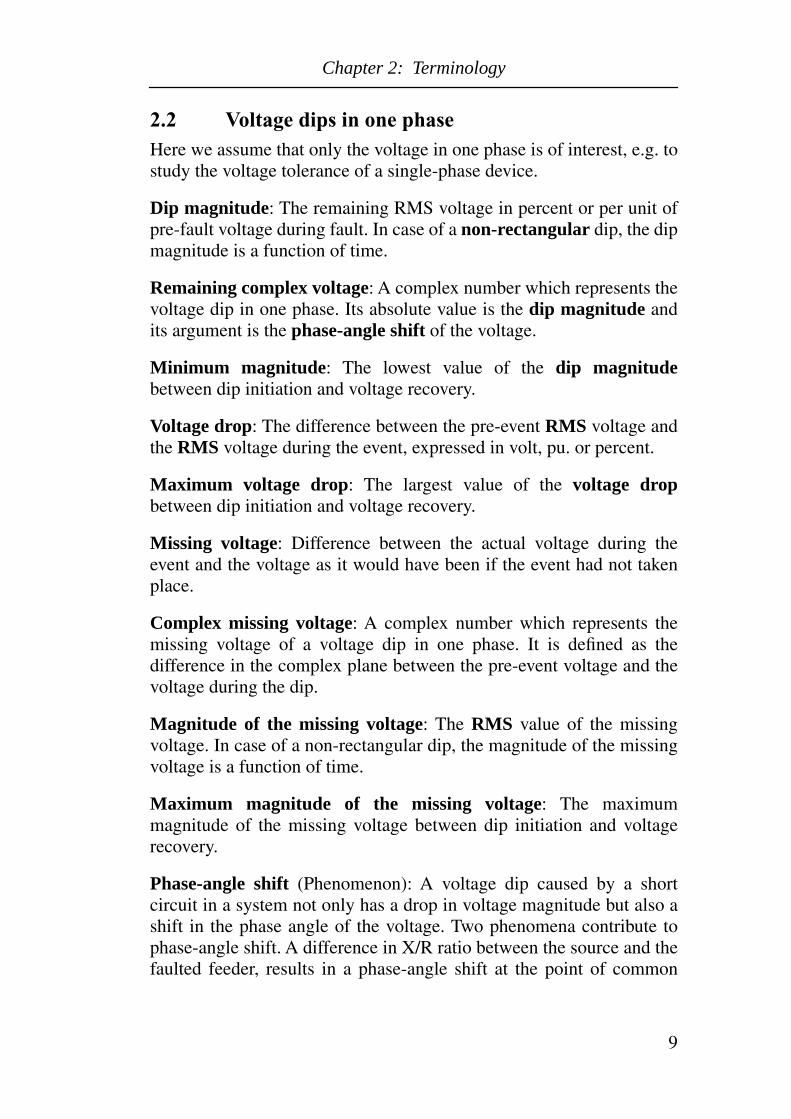
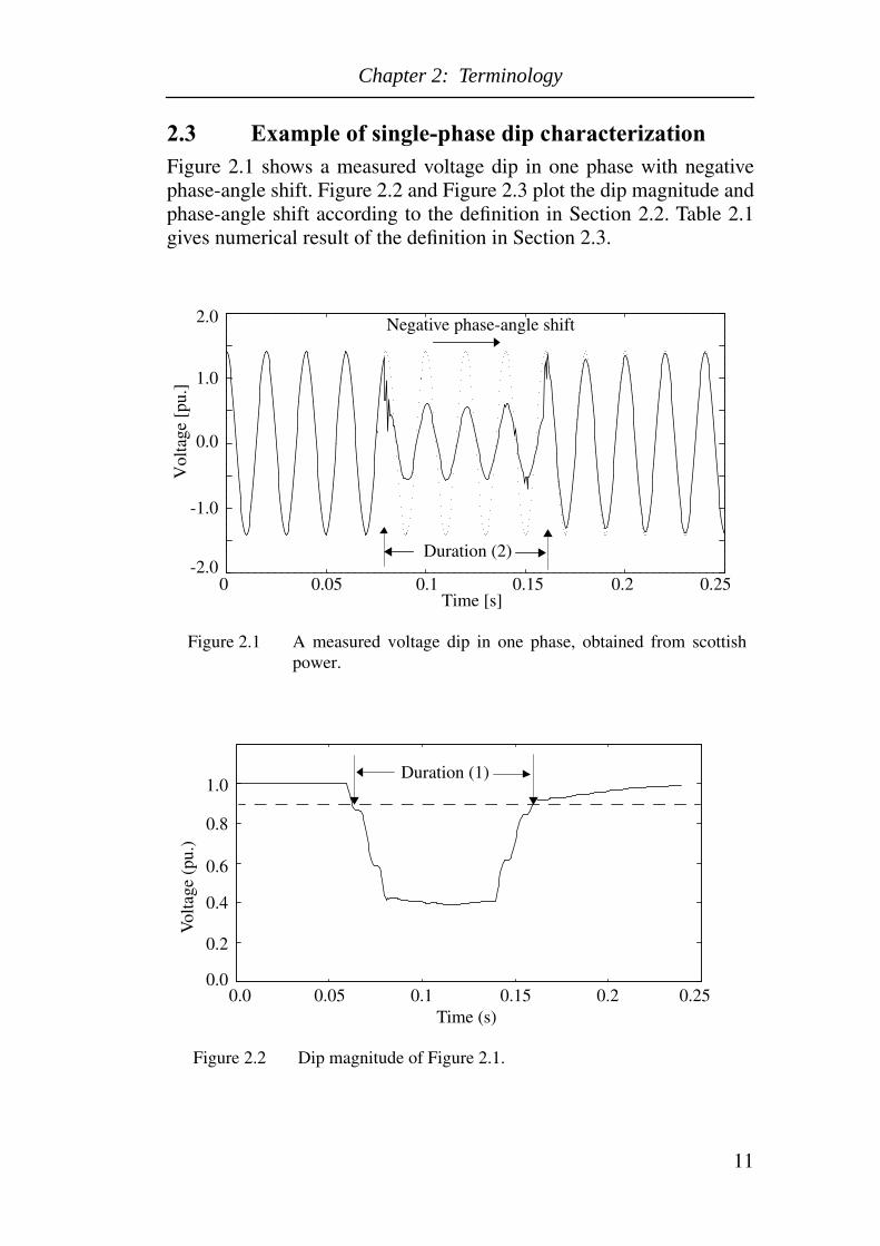
2.3 Example of single-phase dip characterizationFigure 2.1 shows a measured voltage dip in one phase with negativephase-angle shift. Figure 2.2 and Figure 2.3 plot the dip magnitude andphase-angle shift according to the definition in Section 2.2. Table 2.1gives numerical result of the definition in Section 2.3.
Duration (2)
Negative phase-angle shift
Figure 2.1 A measured voltage dip in one phase, obtained from scottishpower.
0 0.05 0.1 0.15 0.2 0.25-2.0
-1.0
0.0
1.0
2.0
Time [s]
Vol
tage
[pu
.]
0.0 0.05 0.1 0.15 0.2 0.25
0.2
0.6
0.8
1.0
0.4
0.0
Vol
tage
(pu
.)
Time (s)
Duration (1)
Figure 2.2 Dip magnitude of Figure 2.1.

Chapter 2: Terminology
12
The dip magnitude in Figure 2.2 is calculated as the RMS voltage overa window of one cycle, which was 96 samples for the recording used.Each point in Figure 2.2 is the RMS voltage over the preceding 96points:
(2.1)
with N = 96 and vi the sampled voltage in time domain.
The phase-angle shift in Figure 2.3 is obtained from the phase angle ofthe fundamental component of the voltage compared to the pre-faultvoltage. The complex fundamental component was obtained from aFast Fourier Transformation (FFT). Let V(t) be the complexfundamental voltage over the period [t, T] with T one cycle of thefundamental frequency, and V0 be the complex voltage at t = 0. Thesynchronous voltage has an angle φ0 + ωt with ω the angular speed ofthe fundamental frequency. The phase-angle shift ∆φ as plotted inFigure 2.3 can be calculated from:
(2.2)
The oscillation of the phase angle around dip initiation and voltagerecovery are due to the shift of the window in and out of the dip. Ittakes one cycle before the phase-angle shift reaches a reliable value. In
0 0.05 0.1 0.15 0.2 0.25-30
-20
-10
0
10
Time (s)
Phas
e-an
gle
shif
t (de
gree
)
Figure 2.3 Phase-angle shift of the dip in figure 2.1
Vrms k( ) 1N---- vi
2
i k N– 1+=
i k=
∑=
∆φ V t( )
V0ejwt
-----------------
arg=

Chapter 2: Terminology
13
calculating the maximum phase-angle shift listed in Table 2.1, theoscillation areas are skipped.
Table 2.1: Numerical characterization results of dip in Figure 2.1
Some comments on the definition of characteristics for dips in a singlephase:
1. In IEC standards and UNIPEDE documents, the severity of a dip isquantified by the voltage drop during the dip [9][17], while in IEEEstandards the magnitude refers to the remaining magnitude during thedip [8]. In IEC 61000-4-11[10], another term, “test level”,corresponding to the IEEE definition magnitude, is used. Themagnitude of a dip can be described as a percentage of nominal voltageor as a percentage of pre-fault voltage. In analysing voltage dipmeasurement and assessing appropriate voltage regulation at a piece ofequipment, the pre-fault voltage reference is more convenient.However, end-use equipment is rated based on its nameplate rating ornominal voltage, so that nominal voltage is a good measure. Inreporting voltage dips, it is important to clarify the notation used.
2. The RMS plot of dip magnitude (Figure 2.2) uses a one cyclemoving window for the calculation. Although the actual waveformdrops rather abruptly, the RMS voltage shows a smooth transition to itsduring-event value. The same phenomenon occurs upon recovery.Thus, the duration (1) defined by RMS drop over-estimates the dipduration by up to one half cycle. The similar phenomenon occurs forthe phase-angle shift, with an oscillation occurs during the transition.The phase-angle is obtained by FFT with a one-cycle moving window.
Definition Value Definition Value
Minimum dip magnitude (pu.)
0.3884 Dip duration (2) (time,second)
0.09
Maximum voltage drop (pu.)
0.6116 Point-on-wave of initiation (time, second)
0.079
Maximum missing voltage (pu.)
0.6235 Point-on-wave of initiation (degree, angle)
860
Maximum phase-angle shift (degree)
-130 Point-on-wave of recovery (time, second)
0.169
Dip duration (1) 0.097 Point-on-wave of recovery (degree, angle)
750

Chapter 2: Terminology
14
3. Duration (2), defined by the point-on-wave gives a better estimationof the exact time that the fault lasts. But duration (2) under-estimatesthe dip duration in case the event is associated with a deep post-faultdip.
4. Dip magnitude and voltage drop are two opposite ways to describethe severity of a dip. Their absolute value addition is equal to the pre-fault voltage, which is assumed to be 1 pu.
5. Remaining complex voltage and complex missing voltage are twoopposite ways to describe the severity of a dip. Their vector addition isequal to the pre-fault voltage, which is assumed to be 1 pu.
dip magnitude
voltage drop
pre-fault voltage
dip magnitude
missing voltage
remaining voltagemissing voltage
Figure 2.4 Phasor relationship of complex remaining voltage andcomplex missing voltage. Bold --- complex number, Italic ---scalar number.

Chapter 3: Classification of Three-phase Voltage Dips
15
Chapter 3 Classification of Three-phase Voltage Dips
Voltage dips are mainly caused by short circuit faults in power systems.In this chapter, a simple voltage divider model is used to illustrate theshort circuits and voltage dips, and how this leads to a drop in rmsvoltage and a phase-angle shift. Dips caused by unbalanced faults areanalyzed by symmetrical components. Based on the fault analysisusing symmetrical components, a classification of three-phase voltagedips is introduced. Mathematical models for transformers aredeveloped to study the changes in the dip characteristics when a dipgoes through a transformer. Finally, the terminology related to three-phase dips is defined as a complement of Chapter 2.
3.1 Balanced faults
To explain the origin of voltage dips and the associated phase-angleshifts due to a system fault, a voltage divider model is often used. Thevoltage divider is shown in Figure 3.1.
Assuming that a three-phase fault(3Ø) occurs at position F, the(complex) voltage remaining at the point-of-common coupling (PCC)during the fault is
(3.1)
Figure 3.1 Voltage divider model
PCC
F
Load
ZfZs
Vdip
ZfZs Zf+------------------= pu.

Chapter 3: Classification of Three-phase Voltage Dips
16
where Zf is the feeder impedance, and Zs is the source impedance. Thepre-fault voltage is here assumed to be .
Besides the voltage drop (the absolute value of Vdip), there is oftenphase-angle shift present. The origin of the phase-angle shift can beunderstood as follows:
Let
(3.2)
and
(3.3)
The argument of the remaining complex voltage is
(3.4)
The argument of expression (3.4) is the difference between the pre-fault and the during-fault voltage phase angle. Due to the symmetry ofthe three-phases during a 3Ø, we can easily introduce a phasor. We willuse the term characteristic voltage, for the remaining complexvoltage, Vdip in (3.1). Note that the remaining complex voltages are thesame in all three phases during a three-phase fault to quantify abalanced voltage dip.
The magnitude of a dip depends on the distance between the fault andthe PCC and on the fault level at PCC. A stronger system, where Zs issmaller, results in an increase of the dip magnitude (a less severeevent). The phase-angle shift associated with a dip is determined by theX/R ratio difference between the source and the feeder. In adistribution system, the feeder has a smaller X/R ratio compared to thesource. Thus a negative phase-angle shift is often accompanying a dipdue to a fault in distribution systems.
In a mesh-connected network, such as in transmission systems, theconcept of voltage divider model is still useful [3]. However, thefeeders and the source impedance are not easy to identify. Thisnormally requires a computer program for network fault analysis. Intransmission systems, there is no big difference in the X/R ratio
1 00∠
ZS RS jXS+=
Zf Rf jXf+=
∆Φ arcXf
Rf------
tan arcXS Xf+
RS Rf+-------------------
tan–=
Chapter 3: Classification of Three-phase Voltage Dips
17
between the source and the feeders. Thus no significant phase-angleshifts occur for balanced dips due to faults on transmission lines.
3.2 Unbalanced faultsThe three phase voltages during an unbalanced system fault generallyshow different magnitudes and phase-angle shifts. Furthermore, thethree phase quantities show different changes when they move throughvarious types of transformers and load connections [6]. Thus we cannot directly use any single one of the three phase voltages to quantifyan unbalanced dip.
3.2.1 Two-component symmetrical components
The method of two-component symmetrical components is proposedby P.M. Andersson in [12] to simplify calculations by reducing thenumbers of components. The traditional symmetrical componentmethod (also called three-component method) requires three values,where the two-component method only needs two. The two-componentmethod is based on the idea that the positive- and negative- sourceimpedance are equal (Zs1 = Zs2). This assumption holds for any staticcircuit, such as transmission lines and transformers. It is not fullycorrect for synchronous or induction motors. However, since theinfluence of rotating machines on the source impedance is usuallysmall, the positive- and negative-sequence source impedance are nearlyequal in reality.
In the theory of symmetrical components, three sequence networks,positive-, negative-, and zero-sequence networks are defined under theunbalanced situation, as shown in Figure 3.2.

Chapter 3: Classification of Three-phase Voltage Dips
18
where Va1, Ia1, and Zs1 represent the positive-sequence voltage,current, and source impedance; Va2, Ia2, Zs2 represent the negative-sequence voltage, current, source impedance; Va0, Ia0, and Zs0represent the zero-sequence voltage, current, and source impedance. Fis the fault point and N is the “zero-potential bus”. VF is the pre-faultvoltage of phase a at F.
The relations among them can be written in matrix form
(3.5)
Under the assumption
(3.6)
Equation (3.5) can be re-written, by adding and subtracting the secondand third rows, as
(3.7)
+-VF
N0
Zs1
F1
N2
ZERO POSITIVE NEGATIVE
Figure 3.2 Sequence networks with defined sequence quantities.
F0 F2
Zs2Zs0
N1
++
- - -
+
-
Va0 Va1 Va2
Ia0 Ia1 Ia2
Va0
Va1
Va2
0
VF
0
Zs0 0 0
0 Zs1 0
0 0 Zs2
Ia0
Ia1
Ia2
–=
Zs1 Zs2=
Va0
Va1 Va2+
Va1 Va2–
0
VF
VF
Z0 0 0
0 Zs1 0
0 0 Zs1
Ia0
Ia1 Ia2+
Ia1 Ia2–
–=

Chapter 3: Classification of Three-phase Voltage Dips
19
These Equations are interesting because the last two rows are bothpositive-sequence Equations.
For convenience we define the sum and difference quantities
(3.8)
The “analysis equation” and “synthesis equation” for two-componentmethod can also be derived.
From the “analysis equation” of the three-component symmetricalcomponent method,
(3.9)
where
the new “analysis equation” is derived by adding and subtracting thesecond and third rows of Equation (3.9)
(3.10)
Va0
VaΣVa∆
Va0
Va1 Va2+
Va1 Va2–
≡
Va0
Va1
Va2
1 1 1
1 a a2
1 a2
a
Va
Vb
Vc
=
a 12---– j
32
-------+=
Va0
VaΣVa∆
13---
1 1 1
2 1– 1–
0 j 3 j 3–
Va
Vb
Vc
=

Chapter 3: Classification of Three-phase Voltage Dips
20
accordingly the “synthesis equation”
(3.11)
can be also written as
(3.12)
The derivation of Equations for currents follow the same procedure asvoltages.
3.2.2 Unbalanced faults analysis by sequence networks
Under two-component symmetrical components, sequence networkscan be constructed for different kinds of shunt faults in power systems.Detailed construction procedure can be found in [12].
The point for analysis is chosen at PCC in Figure 3.1, that is to say, weanalyze Va0, VaΣ, and Va∆ at PCC.
a. The single-line-to-ground fault (SLGF)
Va
Vb
Vc
1 1 1
1 a2
a
1 a a2
Va0
Va1
Va2
=
Va
Vb
Vc
1 1 0
1 12---– j
32
-------–
1 12---– j
32
-------
Va0
VaΣVa∆
=

Chapter 3: Classification of Three-phase Voltage Dips
21
b. The line-to-line fault (LLF)
c. The double-line-to-ground fault (2LGF)
Figure 3.3 Sequence network connections at PCC for a single-line-to-ground fault on phase a.
+
-
-
+
-
P1
Va∆VF
Zs1
N1
Ia∆ 0=
P1
Zs1
VF
IaΣ 2Ia0=
VaΣ
Va0Zs0
2------------
N0
N1
2Ia0
IaΣ
P0
+
-
++
-
Zf1Zf0
2---------+
Figure 3.4 Sequence network connections for a line-to-line fault on phaseb and c.
+
--
+
P1
VaΣVF
Zs1
N1
IaΣ 0=
+
--
+
P1
Va∆VF
Zs1
N1
Ia∆
Zf1

Chapter 3: Classification of Three-phase Voltage Dips
22
3.3 Definition of dip typesIn Section 3.2, Equation (3.12) shows that three-phase unbalancedvoltages can be characterized through three sequence values Va0, Va∆,and VaΣ. Under the assumption of (3.6), both Va∆ and VaΣ are positive-sequence quantities. That is, both the sigma and delta quantities aredefined as voltages or currents associated with the same positive-sequence network. The number of networks is reduced from three totwo.
The zero-sequence voltage does not need to be considered in three-phase voltage dips. Two reasons for this can be given: 1) The zero-sequence voltage usually equals zero at the equipment terminals, sinceit does not pass a delta-star, delta-delta, or ungrounded star-starconnection transformer. 2) Three-phase equipment is normally delta-connected or ungrounded star-connected, so that the zero-sequencevoltage over the equipment terminals is zero.
3.3.1 The single-line-to-ground fault (SLGF)
The sequence network for the SLGF as shown in Figure 3.3 shows aninteresting result: where Va∆ is always equal to the pre-fault voltage VF,independent of the position of the fault. Thus VaΣ is the only quantity
Figure 3.5 Sequence network connections for a double-line-to-ground faulton phase b and c.
+
--
+
P1
VaΣVF
Zs1
N1
Ia∆
+
--
+
P1
Va∆VF
Zs1
N1
Ia∆
Zf1 +
-
2Va02Zs0N0
Ia0P0
Zf1+2Zf0

Chapter 3: Classification of Three-phase Voltage Dips
23
subject to change. In other words, the dip can be characterized fully byVaΣ only. Of course, two-component symmetrical components arebased on the assumption Zs1 = Zs2. These two values are never exactlyequal in reality. We therefore introduce the so-called “positive-negativefactor” (PN-factor) which is equal to Va∆ for a SLGF. The PN-Factoris equal to the pre-fault voltage if the positive- and negative- sequencesource impedances are the same.
Voltage dips due to single-line-to-ground faults were earlier defined astype D[6]. The three voltage phasors for a voltage dip of type D withcharacteristic voltage V and PN-factor F, are given as follows:
(3.13)
These expressions are obtained by filling in, Va0 = 0, Va∆ = F, VaΣ= V,in (3.12).
For Zs1 = Zs2, the earlier analysis leads to F = 1, after which (3.13)becomes identical to the expression for a type D dip in [6]. Thus theearlier classification implicitly assumed equal positive- and negative-sequence impedances. V is the only variable if PN-factor F equals to 1.V is called the characteristic voltage of type D.
A single-line-to-ground fault generates a dip of type D at PCC, wherethe characteristic voltage has the following expression:
(3.14)
Note that the characteristic voltage for a dip due to a three-phase fault,would be:
(3.15)
Va V=
Vb12---V–
12--- jF 3–=
Vc12---V–
12--- jF 3+=
VZf1
Zs0 Zf0+
2-----------------------+
Zs1 Zf1
Zs0 Zf0+
2-----------------------+
+
----------------------------------------------------------- VF⋅=
V3∅Zf1
Zs1 Zf1+----------------------- VF⋅=

Chapter 3: Classification of Three-phase Voltage Dips
24
A SLGF fault gives a higher value for characteristic magnitude than a3Ø fault. The difference can be thought as due to an additionalimpedance (Zs0 + Zf0)/2 between the PCC and the fault.
3.3.2 The line-to-line fault (LLF)
The sequence network for the LLF as shown in Figure 3.4 also showsthat VaΣ is equal to the pre-fault voltage. These dips can be fullycharacterized by Va∆ only. For these dips we define the characteristicvoltage V as Va∆ and the PN-factor F as VaΣ. Voltage dips due to LLFfaults were earlier defined as type C [6]. The three voltage phasors for avoltage dip of type C with characteristic magnitude V and PN-factor F,are given as follows:
(3.16)
These expressions are obtained by filling in, Vao = 0, Va∆ = V, VaΣ= F,in (3.12).
For Zs1 = Zs2, the earlier analysis leads to F = 1, after which (3.16)becomes identical to the expression for a type C dip in [6]. Thus theearlier classification implicitly assumed equal positive- and negative-sequence impedances. V is the only variable if PN-factor F equals to 1.V is called the characteristic voltage of type C.
A line-to-line fault generate a dip of type C at the PCC, where thecharacteristic voltage V is given by the following expression:
(3.17)
Note that the characteristic voltage for a dip due to a LLF fault is equalto the characteristic voltage for a dip due to a three-phase fault. Thisdoesn’t imply that the severitie of the events are the same: differentfault types lead to different dip types.
Va F=
Vb12---F–
12--- jV 3–=
Vc12---F–
12--- jV 3+=
VZf1
Zs1 Zf1+----------------------- VF⋅=
Chapter 3: Classification of Three-phase Voltage Dips
25
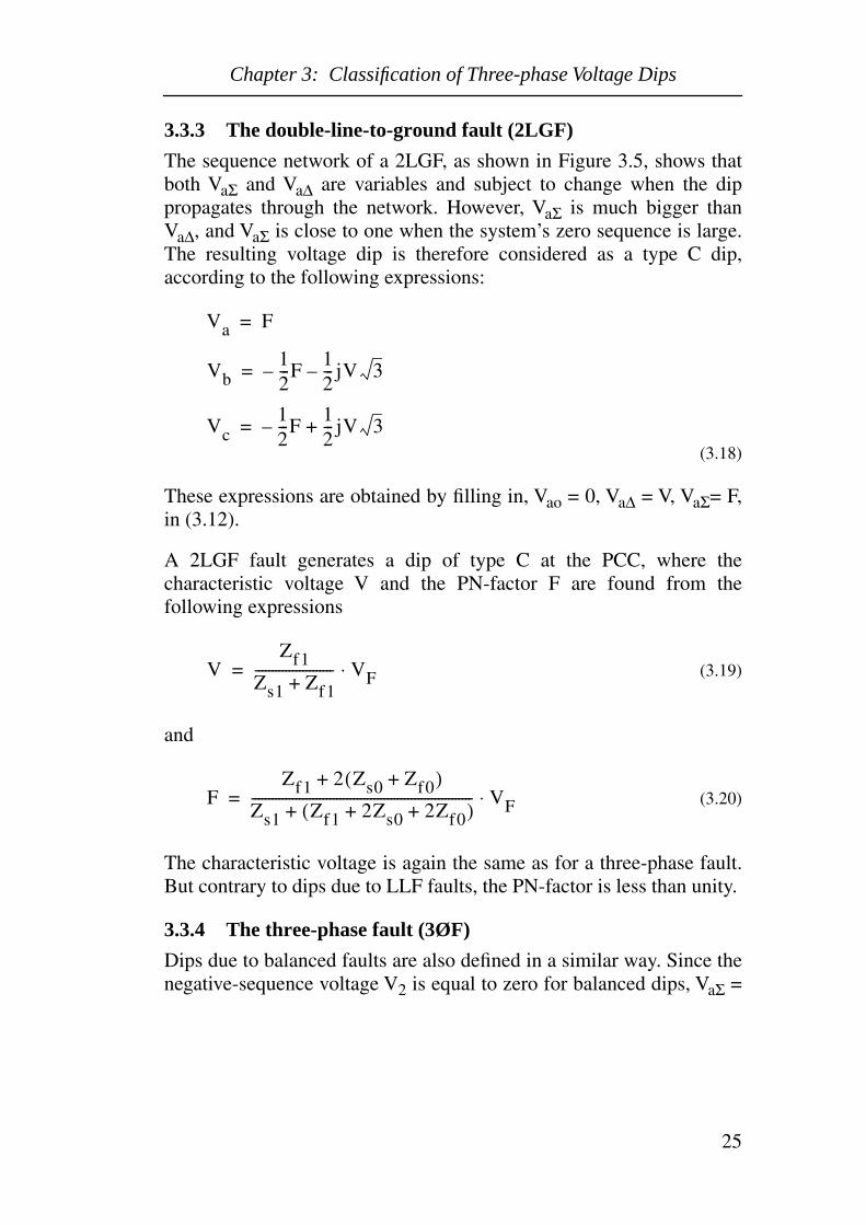
3.3.3 The double-line-to-ground fault (2LGF)
The sequence network of a 2LGF, as shown in Figure 3.5, shows thatboth VaΣ and Va∆ are variables and subject to change when the dippropagates through the network. However, VaΣ is much bigger thanVa∆, and VaΣ is close to one when the system’s zero sequence is large.The resulting voltage dip is therefore considered as a type C dip,according to the following expressions:
(3.18)
These expressions are obtained by filling in, Vao = 0, Va∆ = V, VaΣ= F,in (3.12).
A 2LGF fault generates a dip of type C at the PCC, where thecharacteristic voltage V and the PN-factor F are found from thefollowing expressions
(3.19)
and
(3.20)
The characteristic voltage is again the same as for a three-phase fault.But contrary to dips due to LLF faults, the PN-factor is less than unity.
3.3.4 The three-phase fault (3ØF)
Dips due to balanced faults are also defined in a similar way. Since thenegative-sequence voltage V2 is equal to zero for balanced dips, VaΣ =
Va F=
Vb12---F–
12--- jV 3–=
Vc12---F–
12--- jV 3+=
VZf1
Zs1 Zf1+----------------------- VF⋅=
FZf1 2 Zs0 Zf0+( )+
Zs1 Zf1 2Zs0 2Zf0+ +( )+----------------------------------------------------------------- VF⋅=

Chapter 3: Classification of Three-phase Voltage Dips
26
Va∆ = V1. These kinds of dips are defined as type A. The phasorvoltages for dips of type A are given by the following expressions:
(3.21)
Equation (3.21) is also obtained from equation (3.12) by substitutingVao = 0, Va∆ =VaΣ = V. V is the only variable in equation (3.21). V iscalled the characteristic voltage of type A.
A 3ØF fault generates a dip of type A at the PCC, where thecharacteristic voltage V is found from the following expressions
(3.22)
Figure 3.6 shows the phasor diagram of three different types of dips,given a PN-factor equals to 1 for unbalanced dips, and a characteristicvoltage equal to 0.5∠00 for each type.
The definitions of dip types were first introduced by [6], where fourtypes of dips, type A, B, C, D were defined. The dip types as defined inthis section are a generalisation based on symmetrical components. Anadditional PN-factor F is introduced in type C and type D to include
Va V=
Vb12---V–
12--- j 3V–=
Vc12---V–
12--- j 3V+=
VZf1
Zs1 Zf1+----------------------- VF⋅=
Figure 3.6 Phasor diagram of the three types of voltage dips. PN-factor F= 1.0, zero-sequence voltage Va0 = 0.0, characteristic voltage V= 0.5∠00. Dashed line: the pre-fault phase voltages; solid line:phase voltages during the dip.
Type A Type C Type D

Chapter 3: Classification of Three-phase Voltage Dips
27
the situation where positive- and negative-sequence source impedancesare not equal. Type B is a special case of type D which holds for zero-sequence impedance equal to positive-sequence impedance. Thisassumption generally doesn’t hold in power systems. In the proposedclassification, this type is considered as type D without specialconsideration.
3.3.5 Overview of the classification
In the previous sections, a classification of three-phase unbalanced dipsinto three types, is introduced. The classification is based on thevoltage components VaΣ and Va∆(being sum and difference,respectively of positive- and negative-sequence voltage). For a dip oftype A, VaΣ and Va∆ are equal; for a dip of type C, VaΣ is equal to thepre-fault voltage and Va∆ is dependent on the distance to the fault. For adip of type D the situation is the other way around. In the ideal case,the three dip types fall on the straight lines in Figure 3.7(a). Due to thevarious assumptions, they fall in the three different areas in Figure3.7(b). In Figure 3.7 (b), the normal operation and interruption are alsoincluded as voltage dips in general. The determined value ischaracteristic voltage V (VaΣ in type D and Va∆ in type C). The normaloperation state corresponds to voltage dips (Type A, C, D) wherecharacteristic magnitude |V| is bigger than 90%. The interruptioncorresponds to voltage dips (Type A, C, D) where characteristicmagnitude |V| is smaller than 10%.
The accuracy of the proposed method of dip classification depends onthe correctness of the following three assumptions:
type C
type D
type A
type C
type D
type A
Va∆
VaΣ
Va∆
VaΣ
Figure 3.7 Definition of dip types (a) Dip types in ideal case. (b) Dip typesin general.
(a) (b)
Normal Operation
Interruption
90%
10%

Chapter 3: Classification of Three-phase Voltage Dips
28
1) Zero-sequence voltages do not affect equipment operation.2) Positive- and negative- sequence source impedances don’t differ
much.3) 2LGF faults are rare.
Field measurements, later shown in Chapter 5, show these assumptionsare quite acceptable in reality. Under these assumptions, any three-phase voltage dips can be characterized by one phasor, namely thecharacteristic voltage V. This conclusion greatly simplifies analysis ofthree-phase unbalanced dips. In Chapter 5, the accuracy of theclassification will be further discussed and assessed by field measureddata.
From expressions of the characteristic voltage V for four differenttypes of faults, we notice that, if the fault places are the same, dipsfrom LLF, 3ØF, 2LGF have the same characteristic voltage V at PCC,dips from SLGF have a larger characteristic voltage because of thepresence of the zero-sequence impedance in the sequence network ofthe characteristic voltage V (VaΣ). The presence of the zero-sequenceimpedance also influences the sequence network of the PN-factor F(Va∆) for the dips due to 2LGF.
3.3.6 Phase-angle shift in unbalanced dips
In Section 3.1, we discussed the phase-angle shift associated with abalanced voltage dip. We concluded that the phase-angle shift inbalanced dips is caused by the X/R ratio difference between the sourceand the faulted feeder. Because the X/R ratio of the feeder is generallysmaller than the X/R ratio of the source in distribution systems, weexpect negative phase-angle shifts during a balanced dip. This will beconfirmed by field measurements in Chapter 5.
The X/R ratio difference has the same effect on the characteristicvoltage for unbalanced dips. The argument of the characteristic voltageis non-zero due to a difference of X/R ratio between the source and thefeeder. Dips caused by SLGF show a slightly different behavior sincethe zero-sequence source impedance becomes part of the faultedfeeder. This effect often results in a smaller argument of thecharacteristic voltage.
Besides the effect of X/R ratio difference, there is another effectcausing phase-angle shift in unbalanced dips. As Figure 3.6 shows,while two faulted phases of type C dip tend to come closer to each

Chapter 3: Classification of Three-phase Voltage Dips
29
other, two unfaulted phases of type D tend to go further from eachother. The resulted phase-angle shift of phase voltages in unbalanceddips is an aggregation of these two effects. Substituting the magnitudeand argument of characteristic voltage as a complex number inexpression (3.13) and (3.16), gives the final phase-angle shift on phasevoltages.
3.3.7 Symmetrical phase for unbalanced dips
In previous sections, we only defined unbalanced dips with phase a asthe symmetrical phase, i.e. the fault at phase a for SLGF and a faultbetween phases b and c for LLF and 2LGF. With the consideration ofphase b and phase c as symmetrical phases for Dips of type C and D,the classification results in six different types of dips namely Ca, Cb,Cc, Da, Db, Dc with the subscript indicating the symmetrical phase.Table 3.1 gives the mathematical expressions and Figure 3.8 gives theirphasor diagrams. The mathematical expressions for unbalanced dipswith symmetrical phase b and c are derived by rotating the three-phases of unbalanced dips by 2400 and 1200 respectively. In Table 3.1and Figure 3.8, we assume the PN-factor F of type C and D equals to 1to simplify the expressions.

Chapter 3: Classification of Three-phase Voltage Dips
30
a
b
c
a
b
c
a
b
c
a
b
c
a
b
c
a
b
c
Type CaType Cb Type Cc
Type DaType Db
Type Dc
Figure 3.8 Phasor diagram of unbalanced dips with the consideration ofsymmetrical phases. PN-factor F = 1.0, zero-sequence voltageVa0 = 0.0, characteristic voltage V = 0.5∠00. Dashed line: thepre-fault phase voltage; solid line: phase voltages during dip.

Chapter 3: Classification of Three-phase Voltage Dips
31
Table 3.1: Phase voltages for unbalanced dips
Table 3.2 gives the symmetrical component expressions for the dips inTable 3.1 by using equation (3.9).
Type Ca Type Da
Type Cb Type Db
Type Cc Type Dc
Va 1=
Vb12---–
12--- j 3V–=
Vc12---–
12--- j 3V+=
Va V=
Vb12---V–
12--- j 3–=
Vc12---V–
12--- j 3+=
Va14---
34---V
14--- j 3
14--- jV 3–+ +=
Vb12---–
12--- j 3–=
Vc14---
34---V–
14--- j 3
14--- jV 3+ +=
Va14---V 3
4---
14--- j 3–
14--- jV 3+ +=
Vb12---V–
12--- j 3V–=
Vc14---V 3
4---–
14--- j 3
14--- jV 3+ +=
Va14---V 3
4---
14--- j 3–
14--- jV 3+ +=
Vb14---
34---V–
14--- j 3–
14--- jV 3–=
Vc12---–
12--- j 3+=
Va14---
34---V
14--- j 3
14--- jV 3–+ +=
Vb14---
34---V–
14--- j 3–
14--- jV 3–=
Vc12---V–
12--- jV 3+=

Chapter 3: Classification of Three-phase Voltage Dips
32
Table 3.2: Symmetrical components for the six types of dips
From Table 3.2 it follows that the positive-sequence voltage is alwaysalong the reference phase axis. The direction of the negative-sequencevoltage depends on the type of dip. We also notice that the negative-sequence voltages have opposite direction for type C and type D dipswith the same symmetrical phase. This is consistent with the definitionof the characteristic voltage, which is defined as the subtraction ofpositive- and negative-sequence voltages for type Ca but the addition ofpositive- and negative-sequence voltages for type Da.
Under the generalised definition, these six types of dips have the samecharacteristic voltage. By rotating the negative-sequence voltage overan integer multiple of 600 all dips can be obtained from one prototypedip; dip type Ca has been chosen as the prototype dip. Thus thecharacteristic voltage is obtained by the subtraction of positive andnegative sequence voltage of Ca. Due to the same reason, these sixtypes of dips have the same PN-factor, where it is considered. The PN-factor is obtained by the addition of positive- and negative- sequencevoltages of Ca.
Figure 3.9 shows the phasor diagram for positive- and negative-sequence voltages of the six types of unbalanced dips. While thepositive-sequence voltage is the same for the six types of dips, theargument of the negative sequence determines which type the dip is.
Type Ca Type Da
Type Cb Type Db
Type Cc Type Dc
V11 V+
2-------------=
V21 V–
2-------------=
V11 V+
2-------------=
V21 V–
2-------------–=
V11 V+
2-------------=
V2 a1 V–
2-------------⋅=
V11 V+
2-------------=
V2 a–1 V–
2-------------⋅=
V11 V+
2-------------=
V2 a2 1 V–
2-------------⋅=
V11 V+
2-------------=
V2 a–2 1 V–
2-------------⋅=

Chapter 3: Classification of Three-phase Voltage Dips
33
The algorithm of recognizing dip type from field measurements will bestudied in detail in Chapter 5.
3.4 Dip transformation through transformersTransformers come with many different winding connections. As avoltage dip passes through a transformer, the phasors’ relation of thevoltage dip at the secondary side of the transformer will becomesdifferent compared to the voltage dip at the primary side. In theconcept of dip classification, the type of dip could change. In thissection, we intend to build the mathematic models, in matrix form, forvarious types of transformers in this section for modelling the change,that is, the phasors of the voltage dip at the secondary side shall beobtained by multiplying the phasors of the voltage dip at the primaryside with the matrix of the transformer. The load current is ignored inthe analysis.
The modelling procedure is taken in two steps:
Cb
Cc
Da
Ca
Db
Dc
Va1
a
b
c
Va2
Figure 3.9 Phasor Diagram of unbalanced dips with symmetricalcomponents, PN-factor F = 1, characteristic voltage V = 0.5∠−300. Dashed line: pre-fault phase voltages.

Chapter 3: Classification of Three-phase Voltage Dips
34
1) The matrix model of the transformer changes voltage phasors, whileretaining the symmetrical phase of the voltage dip. These are calledbasic transformer models.
2) Only the symmetrical phase of the dip is changed. These are calledsymmetry changers.
In Section 3.4.4, We relate the basic transformer model and symmetrychanger to the physical transformers.
3.4.1 Basic transformer models
Three basic transformer models can be distinguished, based on [6]:
1. Transformers where each of the secondary voltages is the differencebetween two primary voltages. These kinds of transformers include Dy,Yd, and Yz connected transformers.
These transformers can be defined mathematically in matrix form, asfollows:
(3.23)
Each phase at the secondary of the transformer is a subtraction of twophases at the primary side of this kind of transformer. The factor isaimed at changing the base of the pu. values. The j is introduced so thatthe symmetrical phase of the dip is maintained.
In symmetrical components, the positive-sequence voltage doesn’tchange through such a transformer model, but the transformer modelreverses the direction of the negative-sequence voltage. Thus a type Cdip will change into a type D dip, and vice versa. This can be illustratedby the following calculations:
Given a set of positive-sequence voltage V1
(3.24)
T1j
3-------
0 1 1–
1– 0 1
1 1– 0
=
3
V1
V
a2V
aV
=

Chapter 3: Classification of Three-phase Voltage Dips
35
and a set of negative-sequence voltage V2
(3.25)
It follows that T1*V1 = V1, but T1*V2 = -V2.
The zero-sequence voltage is removed, given
(3.26)
it follows that T1*V0 = 0.
2. Transformers that only remove the zero-sequence voltage. Examplesof this type are the star-star connected transformer with one or both starpoints not grounded (Yny, Yyn), and the delta-delta connectedtransformer (Dd). Also the delta-zigzag (Dz) transformer fits in thiscategory.
This type can be defined mathematically in matrix form, as follows:
(3.27)
Each phase at the secondary side of the transformer is obtained bysubtracting the primary side voltage by the zero-sequence voltage, e.g.
(3.28)
In symmetrical components, such a transformer model changes neitherthe positive-sequence voltage nor the negative-sequence voltage, thatis, T2*V1 = V1, and T2*V2 = V2. But the zero-sequence voltage isremoved, that is, T2*V0 = 0.
V2
V
aV
a2V
=
V0
V
V
V
=
T213---
2 1– 1–
1– 2 1–
1– 1– 2
=
Va′
Va13--- Va Vb Vc+ +( )–=

Chapter 3: Classification of Three-phase Voltage Dips
36
3. Transformers that do not change anything to the voltage. For thistype of transformer the secondary-side voltages (in pu.) are equal to theprimary-side voltages (in pu.). The only type of transformers for whichthis holds is the star-star connected one with both star points grounded(Ynyn).
The mathematical expression for this kind of transformer is simple, itis written as follows:
(3.29)
In symmetrical components, this type of transformer also doesn’tchange anything, that is, T2*V1 = V1, T2*V2 = V2, and T2*V0 = V0.
The effect of three transformer types on sequence voltages can besummarized in Table 3.3.
Table 3.3: The effect of different types of transformer on sequence voltages
3.4.2 Effect of the basic transformer models on the basic dip types
From the analysis of the previous section, T2 and T3 do not affectpositive- and negative-sequence voltages. Voltages of the basic diptypes do only contain positive- and negative-sequence voltages. ThusT2 and T3 will not affect the voltages of the basic dip types. T1 changesthe direction of the complex negative-sequence voltage. From Table3.2, we concluded that the difference between C and D is the sign ofthe negative-sequence voltage. The effect of T1 is thus that type C andD change into each other.
This can be mathematically expressed as follows:
Transformer type Effect on sequence voltages
V0 V1 V2
T1 0 V1 -V2
T2 0 V1 V2
T3 V0 V1 V2
T3
1 0 0
0 1 0
0 0 1
=

Chapter 3: Classification of Three-phase Voltage Dips
37
Given
(3.30)
and
(3.31)
and
(3.32)
Table 3.4 gives the transformation of dips through three kinds oftransformers by multiplying a dip with the matrix model oftransformers, e.g. T1*Da, T2*Ca, etc. Note that the symmetrical phaseis not affected by the basic transformer models.
Table 3.4: Transformation of dip types through transformer
Transformer Connection
Dip type on primary side
A Ca Cb Cc Da Db Dc
T1: Yd, Dy, Yz A Da Db Dc Ca Cb Cc
T2: Yy, Dd, Dz A Ca Cb Cc Da Db Dc
T3: YNyn A Ca Cb Cc Da Db Dc
A
V
12---V–
12--- jV 3–
12---V–
12--- jV 3+
=
Da
V
12---V–
12--- j 3–
12---V–
12--- j 3+
=
Ca
1
12---–
12--- jV 3–
12---–
12--- jV 3+
=

Chapter 3: Classification of Three-phase Voltage Dips
38
Any contents of zero-sequence voltages in type Da or Ca will beremoved by the type T2 transformer but not be affected by T3. A typeT1 transformer changes a type C dip to a type D dip and vice versasince it reverses the direction of the negative-sequence voltage.
3.4.3 Change of the symmetrical phase
The basic transformer models developed in Section 3.4.2 make surethat the transformer doesn’t affect the symmetrical phase of the voltagedip through the transformer. But in reality, a dip could change itssymmetrical phase because of the labelling of the phases at thesecondary side of the transformer (often indicated by the “clocknumber”). e.g. phase A at primary side may corresponds phase b atsecondary side in Wye-Wye connection, or phase A at primary sidemay correspond to phase a-b at secondary side in Wye-delta. We willuse a so-called “symmetry changer” to represent the change ofsymmetrical phase due to a transformer. Symmetry changers can beclassified into three types:
1. Those for which the symmetrical phase rotates clockwise. Phase a,b, c change to phase b, c, a, respectively.
2. Those for which the symmetrical phase rotates in counter-clockwise.Phase a, b, c change to phase c, a, b, respectively.
3. Those that don’t change the symmetrical phase.
They can be written in matrix form, as follows:
(3.33)
(3.34)
S1 a2
0 0 1
1 0 0
0 1 0
=
S2 a0 1 0
0 0 1
1 0 0
=
Chapter 3: Classification of Three-phase Voltage Dips
39
(3.35)
where a = ej120. The operator a and a2 in S1 and S2 are to make surethat the pre-fault voltage, at primary and secondary side of transformer,shows no phase shift. It has a similar function as the j in the expressionfor T1. Table 3.5 shows the change of symmetrical phase through asymmetry changer for the different types of dip.
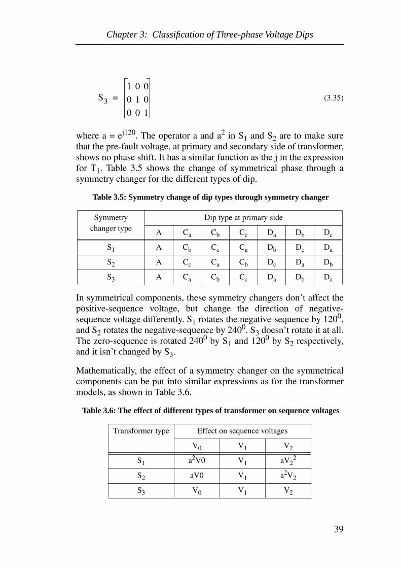
Table 3.5: Symmetry change of dip types through symmetry changer
In symmetrical components, these symmetry changers don’t affect thepositive-sequence voltage, but change the direction of negative-sequence voltage differently. S1 rotates the negative-sequence by 1200,and S2 rotates the negative-sequence by 2400. S3 doesn’t rotate it at all.The zero-sequence is rotated 2400 by S1 and 1200 by S2 respectively,and it isn’t changed by S3.
Mathematically, the effect of a symmetry changer on the symmetricalcomponents can be put into similar expressions as for the transformermodels, as shown in Table 3.6.
Table 3.6: The effect of different types of transformer on sequence voltages
Symmetry changer type
Dip type at primary side
A Ca Cb Cc Da Db Dc
S1 A Cb Cc Ca Db Dc Da
S2 A Cc Ca Cb Dc Da Db
S3 A Ca Cb Cc Da Db Dc
Transformer type Effect on sequence voltages
V0 V1 V2
S1 a2V0 V1 aV22
S2 aV0 V1 a2V2
S3 V0 V1 V2
S3
1 0 0
0 1 0
0 0 1
=
Chapter 3: Classification of Three-phase Voltage Dips
40
Any physical transformer can be represented by a combination of abasic transformer model from Table 3.4 and a symmetry changermodel from Table 3.5. From Table 3.4 and Table 3.5, we conclude diptype A is not affected by any transformer connection. This is quitestraightforward and easy to understand, because a balanced dip keepsthe balance after a delta-star connection and it doesn’t have phasesymmetry. While unbalanced dips may be changed from one type intoanother depending on the transformer’s connection, no new type ofdips is generated.
The concept of transformer model and symmetry changer also applieson the load connection and monitor connection. A delta-connected loadexperiences a type C dip if a star-connected load experiences a type Ddip and vice versa.
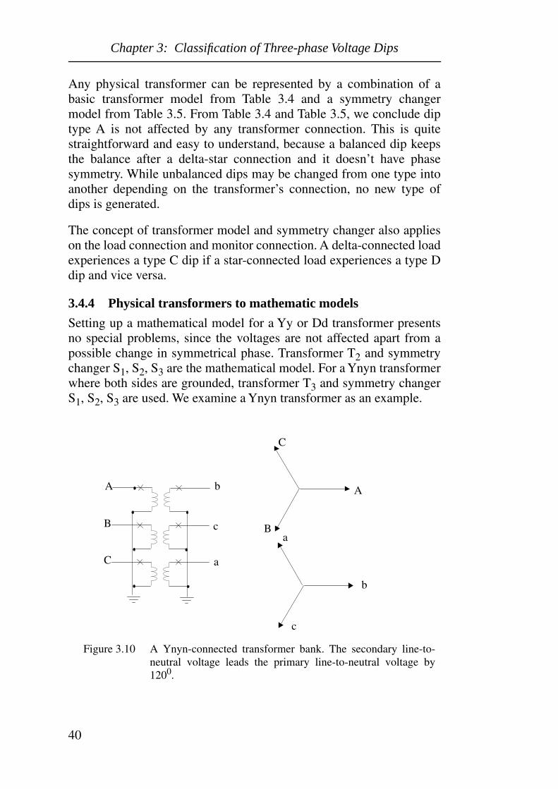
3.4.4 Physical transformers to mathematic models
Setting up a mathematical model for a Yy or Dd transformer presentsno special problems, since the voltages are not affected apart from apossible change in symmetrical phase. Transformer T2 and symmetrychanger S1, S2, S3 are the mathematical model. For a Ynyn transformerwhere both sides are grounded, transformer T3 and symmetry changerS1, S2, S3 are used. We examine a Ynyn transformer as an example.
A
B
C
c
a
Figure 3.10 A Ynyn-connected transformer bank. The secondary line-to-neutral voltage leads the primary line-to-neutral voltage by1200.
A
B
C
b
b
c
a

Chapter 3: Classification of Three-phase Voltage Dips
41
Figure 3.10 shows an Yy-connected transformer bank, where thephases are relabled at the secondary side. The voltage phasor diagramsat the primary and secondary side are also shown in the figure. Thephasor diagram shows that the secondary line-to-neutral voltage leadsthe primary line-to-neutral voltage by 1200.
If the primary voltage is used as the reference, the above transformercan be written mathematically as
(3.36)
In voltage dip study, as we mentioned before, the pre-fault voltage,instead of the primary voltage, is used as the reference. That alsomeans, the positive-sequence voltage will not rotate through thetransformer. In (3.36), there is obvious a 1200 clockwise rotation ofpositive-sequence voltage. Thus an operator a2, that is 1200 counter-clockwise rotation, has to be introduced. Compared to the symmetrychanger model described in Section 3.4.3, this is the same as a S1symmetry changer model.
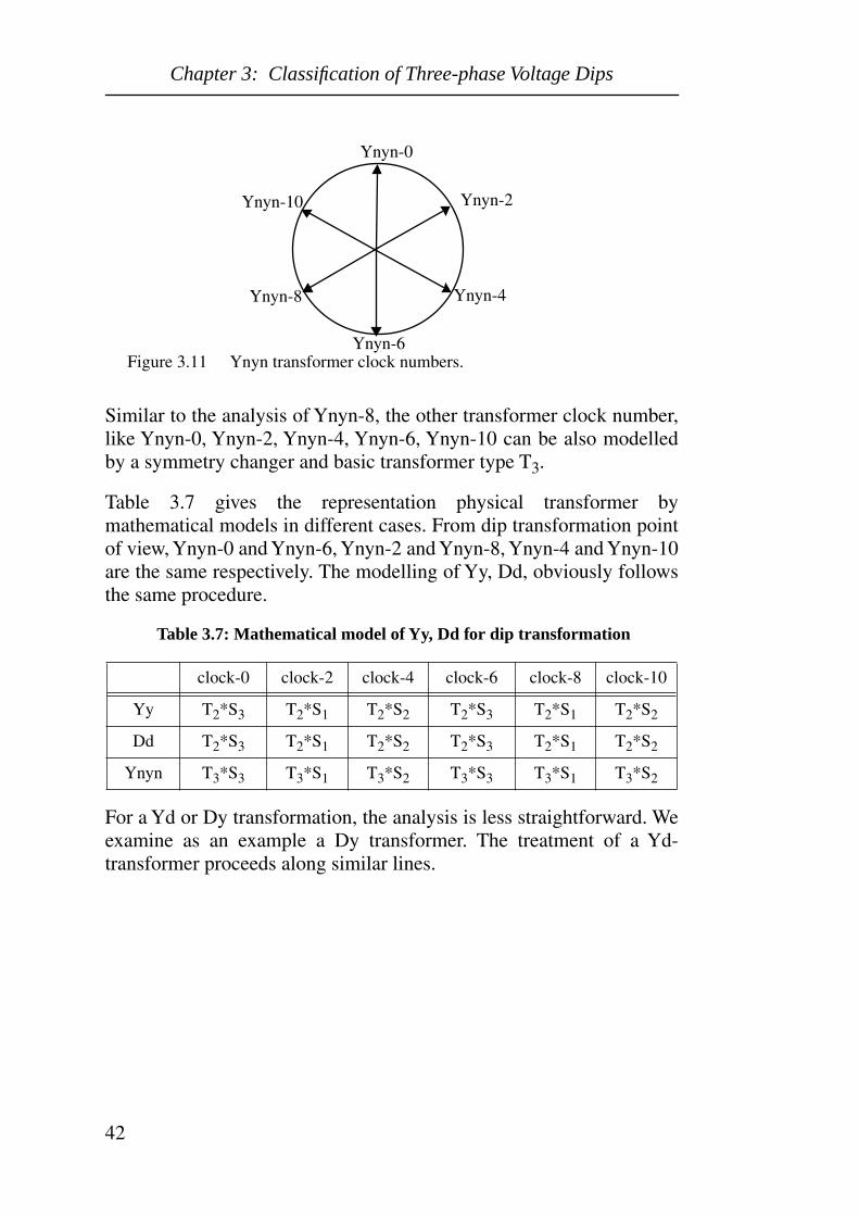
The transformer shown in Figure 3.10 is also called Ynyn-8transformer. The meaning of this notation is as follows: the secondaryvoltage delays the primary voltage by 2400 (or leads by 1200), likeeight o’clock on a clock. Similarly, by changing the transformerconnection, other clock numbers yield, as shown in Figure 3.11.
Va
Vb
Vc
T
VA
VB
VC
with,=
T0 0 1
1 0 0
0 1 0
=
Chapter 3: Classification of Three-phase Voltage Dips
42
Similar to the analysis of Ynyn-8, the other transformer clock number,like Ynyn-0, Ynyn-2, Ynyn-4, Ynyn-6, Ynyn-10 can be also modelledby a symmetry changer and basic transformer type T3.
Table 3.7 gives the representation physical transformer bymathematical models in different cases. From dip transformation pointof view, Ynyn-0 and Ynyn-6, Ynyn-2 and Ynyn-8, Ynyn-4 and Ynyn-10are the same respectively. The modelling of Yy, Dd, obviously followsthe same procedure.
Table 3.7: Mathematical model of Yy, Dd for dip transformation
For a Yd or Dy transformation, the analysis is less straightforward. Weexamine as an example a Dy transformer. The treatment of a Yd-transformer proceeds along similar lines.
clock-0 clock-2 clock-4 clock-6 clock-8 clock-10
Yy T2*S3 T2*S1 T2*S2 T2*S3 T2*S1 T2*S2
Dd T2*S3 T2*S1 T2*S2 T2*S3 T2*S1 T2*S2
Ynyn T3*S3 T3*S1 T3*S2 T3*S3 T3*S1 T3*S2
Ynyn-0
Ynyn-4Ynyn-8
Figure 3.11 Ynyn transformer clock numbers.
Ynyn-2
Ynyn-6
Ynyn-10

Chapter 3: Classification of Three-phase Voltage Dips
43
Figure 3.12 shows an Dy-connected transformer bank and the phasordiagrams at the primary and secondary side. The phasor diagram showsthat the secondary line-to-neutral voltage delays the primary line-to-neutral voltage by 300.
If the primary voltage is used as the reference, the above transformercan be written mathematically as
(3.37)
In voltage dip study, as we mentioned before, the pre-fault voltage,instead of the primary voltage, is used as the reference. That alsomeans, the positive-sequence voltage will not rotate through the
A
B
C
a
b
c
Figure 3.12 A Dy-connected transformer bank. The secondary line-to-neutral voltage delays the primary line-to-neutral voltage by300.
AB
C
a
b
c
Va
Vb
Vc
T
VA
VB
VC
with,=
T1
3-------
1 0 1–
1– 1 0
0 1– 1
=

Chapter 3: Classification of Three-phase Voltage Dips
44
transformer. Applying the transformer model T of (3.37) on thepositive-sequence voltage V1 of (3.24), we get
T*V1 = e-j30*V1 (3.38)
The positive-sequence voltage rotates -300, which is the same as shownby the phasor diagram in Figure 3.12.
To keep the positive-sequence voltage unchanged, a factor ej30 has tobe introduced in (3.37), resulting in (3.39)
(3.39)
Applying the modified transformer model in (3.39) on the negative-sequence voltage V2 of (3.25), we get
T*V2 = e-j60*V2 (3.40)
Comparing with Figure 3.9, we find that, if we keep the positive-sequence voltage and rotate the negative-sequence voltage over -600, atype C dip will change into a type D and vice versa. Besides, thesymmetrical phase a, b, c will change to c, a, b, respectively. This isequivalent to a combination of transformer type T1 and a symmetrychanger S2.
The transformer shown in Figure 3.12 is also called Dy-1 transformer.The meaning of this notation is as follows: the secondary voltagedelays the primary voltage by 300, like one o’clock on a clock.Similarly, by changing the transformer connection, other clocknumbers yield, as shown in Figure 3.13.
Te
j30
3----------
1 0 1–
1– 1 0
0 1– 1
=

Chapter 3: Classification of Three-phase Voltage Dips
45
From symmetrical components point of view, these transformers rotatethe positive-sequence voltage by 300, 900, 1500, 2100, 2700, 3300
clockwise and thus rotates the negative-sequence voltage over the sameangle but in the other direction. If we keep the positive-sequenceunchanged, the negative-sequence will rotate by double the angle. Bycomparing with Figure 3.9, Table 3.8 lists the correspondingmathematical model for voltage dip transformation through differentDy transformers.
Table 3.8: Mathematical models of Dy transformers
From Table 3.8, we can find that the Dy transformer exchange C and Dtype dips, and the different “clock number” only affects thesymmetrical phase. From dip transformation point of view, Dy-1 andDy-7, Dy-3 and Dy-9, Dy-5 and Dy-11 are the same respectively.
Following the similar analysis, we list the results in Table 3.9 for Ydtransformer. It shows the same result as Dy transformers.
Table 3.9: Mathematical model of Yd for dip transformation
Dy-1 Dy-3 Dy-5 Dy-7 Dy-9 Dy-11
T1*S2 T1*S3 T1*S1 T1*S2 T1*S3 T1*S1
Yd-1 Yd-3 Yd-5 Yd-7 Yd-9 Yd-11
T1*S2 T1*S3 T1*S1 T1*S2 T1*S3 T1*S1
Dy-1
Dy-3
Dy-5Dy-7
Dy-9
Dy-11
Figure 3.13 Dy transformer clock numbers.

Chapter 3: Classification of Three-phase Voltage Dips
46
3.5 Terminology: three-phase voltage dipsThree-phase voltage dips: A power quality event in three-phases ofwhich at least one phase shows a decrease in rms voltage outside thenormal operating range. An equal decrease in three-phases is alsocalled a “three-phase balanced dip”, otherwise, “three-phaseunbalanced dip”.
Phase voltage: The remaining complex voltage of each of the threephases in a three-phase unbalanced dip. The absolute values are the dipmagnitudes and the arguments are the phase-angle shifts. This can beeither phase-to-ground or phase-to-phase voltages, depending on theconnection of the equipment.
Dip type: Classification of three-phase voltage dips based on therelations among the three phase voltages. Type A represents a balanceddip. Type D and C represent three-phase unbalanced dips in which oneor two phases drop, respectively. All three types can be quantified byone phasor based on some assumptions. If the symmetrical phase isconsidered, dips of type C and D can be further classified as six types,namely Ca, Cb, Cc, Da, Db, Dc. Unbalanced dips can change into eachother through different kinds of transformer connections.
Characteristic voltage: The phasor which is used to quantify theseverity of a three-phase voltage dip. For balanced dips, type A, itequals to the phase voltage. For unbalanced dips, type C and type D, itdefines as the subtraction of positive-sequence voltage and negative-sequence voltage of type Ca. By knowing the characteristic voltage anddip type, one can reproduce the three-phase voltages of the dip with areasonable level of accuracy. The absolute value is called thecharacteristic magnitude and the argument is called the characteristicphase-angle shift.
Positive and negative factor (PN-Factor): An additional phasor toquantify a three-phase unbalanced dip where the system’s positive- andnegative-sequence impedance are not equal. It is close to unity if thedynamic loads are less connected to the grid. The PN-Factor alsoindicates the degree to which the phase voltages can be reproduced byusing the characteristic voltage alone.
Zero-sequence component voltage: The addition of three-phasevoltages of three-phase voltage dips. In most cases the zero-sequencevoltage component of a three-phase unbalanced dip is zero, but in somecases this additional characteristic is needed.

Chapter 4: Voltage Dip Propagation in Power Systems
47
Chapter 4 Voltage Dip Propagation in Power Systems
One reason that voltage dips have become a serious concern for theindustry is their propagation through the power system. Interruptionsoccur only when a protective device actually interrupts the circuitserving a particular customer. On the other hand, a short-circuit faultcan generate dips over a wide part of the power system.
There are three different types of dip propagation in power systems,which are shown in Figure 4.1.
(I) Propagation at the same voltage level.(II) Propagation to a higher voltage level (or: towards the source).(III) Propagation to a lower voltage level (or: towards the load).
For faults on distribution feeders, propagation types (II) and (III) areimportant. For transmission system faults, type (I) and (III) need to beconsidered.
In Chapter 3, we analyzed the characteristics of three-phase voltagedips resulting from different types of system faults, by using a simplevoltage divider model. Based on a method of two-componentsymmetrical components and a few assumptions, we classified the dips
I
II
III
III
Figure 4.1 Various types of dip propagation in power systems.
Fault

Chapter 4: Voltage Dip Propagation in Power Systems
48
as different types at the PCC. An important result obtained from theclassification is that all three-phase voltage dips, balanced orunbalanced, can be quantified by one phasor, namely the characteristicvoltage. The next question is: what will happen to the dip type andcharacteristic voltage when the dip propagates from the PCC to theequipment terminal?
The study of voltage dip propagation is the basic for stochasticprediction of voltage dips in a certain area. International standards andpublications suggest several methods to predict voltage dips based onhistorical fault statistics and the knowledge of dip propagation [3][5].However, these methods mostly assume a balanced dip. Moreinformation about unbalanced dip propagation is still needed.
In this chapter, we will look at the propagation of voltage dips indistribution systems and transmission systems. Simulations areperformed on two hypothetical power networks, a radial system and aloop system. Based on symmetrical component analysis, a method ofstudying voltage dips by a single-phase scheme for unbalancedsituation is proposed. Finally, the influence of dynamic loads, e.g.induction motors, on the characteristics of dips is discussed.
4.1 Voltage dip propagation in distribution systemsThe radial layout is most often used in distribution network design. Themajor advantages of the radial layout are that it is simpler and moreeconomical to install than other types of layout. Figure 4.2 shows anexample radial system, which transports power from 132 kV leveldown to the loads connected at different voltage levels. Table 4.1- 4.3give the parameters of the power source, transformers and feeders. Thetotal load connected to each bus is approximately 6% of the shortcircuit power for that bus. The loads are assumed pure impedance withpower factor 0.9. Such arrangement makes sure that the system’spositive-sequence and negative-sequence source impedances are equal.The system’s parameters are obtained from [38].
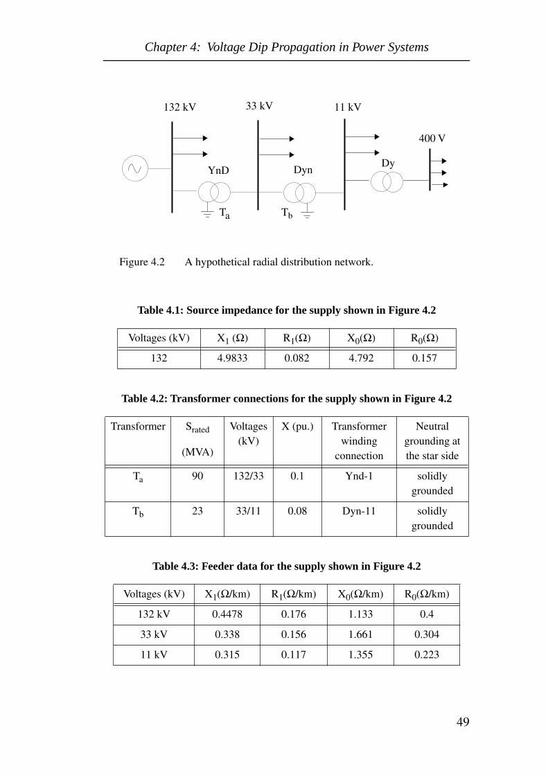
Chapter 4: Voltage Dip Propagation in Power Systems
49
Table 4.1: Source impedance for the supply shown in Figure 4.2
Table 4.2: Transformer connections for the supply shown in Figure 4.2
Table 4.3: Feeder data for the supply shown in Figure 4.2
Voltages (kV) X1 (Ω) R1(Ω) X0(Ω) R0(Ω)
132 4.9833 0.082 4.792 0.157
Transformer Srated
(MVA)
Voltages (kV)
X (pu.) Transformer winding
connection
Neutral grounding at the star side
Ta 90 132/33 0.1 Ynd-1 solidly grounded
Tb 23 33/11 0.08 Dyn-11 solidly grounded
Voltages (kV) X1(Ω/km) R1(Ω/km) X0(Ω/km) R0(Ω/km)
132 kV 0.4478 0.176 1.133 0.4
33 kV 0.338 0.156 1.661 0.304
11 kV 0.315 0.117 1.355 0.223
Figure 4.2 A hypothetical radial distribution network.
132 kV 33 kV 11 kV
Ta Tb
YnD DynDy
400 V

Chapter 4: Voltage Dip Propagation in Power Systems
50
4.1.1 Voltage dip propagates upwards and downwards
Generally a dip originated from a higher voltage level propagatesdownwards to a lower voltage level without main change in magnitude,but the voltage drop is reduced greatly when it propagates from a lowerlevel to a higher level. This effect can be illustrated by the followingsimple calculation:
Naming Xs132 the short-circuit impedance at the 132kV voltage busbarin Figure 4.2, Xt the reactance of the transformer Ta. For three-phaseshort circuit at 33 kV busbar, the characteristic voltage at 33kV equalszero. The dip magnitude at 132 kV is:
(4.1)
Using the values in Table 4.1 through 4.3, the dip magnitude isapproximately 80%.
Simulations are performed for different types of faults on the feeders at2km from the 132 kV, 33 kV, 11 kV busbar. Table 4.4 gives the resultfor the dips measured at each bus. Figures 4.3 through 4.5 show thecharacteristic magnitude and PN-factor at each bus for four differentfault types.
V132
XtXs132 Xt+--------------------------=

Chapter 4: Voltage Dip Propagation in Power Systems
51
Table 4.4: Simulation Results
* V
---
Cha
ract
eris
tic V
olta
ge**
F -
- PN
-fac
tor
Fault Location
Faul
t ty
pe
Cha
ract
eris
tics
of v
olta
ge d
ips
mea
sure
d at
eac
h bu
s
132k
V33
kV
11 k
V
Dip
Ty
peV
*F*
*V
0***
Dip
Ty
peV
FV
0D
ip
Type
VF
V0
132 kV feeder
SLG
FD
a0.
41∠
−40
1.0∠
0.00
0.23
∠−1
750
Cc
0.41
∠−4
01.
0∠0.
000.
0D
a0.
41∠
−40
1.0∠
0.00
0.0
LL
FC
a0.
17∠
−150
1.0∠
0.00
0.0
Dc
0.17
∠−1
501.
0∠0.
000.
0C
a0.
17∠
−150
1.0∠
0.00
0.0
2LG
FC
a0.
17∠
−150
0.68
∠00
0.25
∠40
Dc
0.17
∠−1
500.
68∠
0.00
0.0
Ca
0.17
∠−1
500.
68∠
0.00
0.0
3ØF
A0.
17∠
−150
--0.
0A
0.17
∠−1
50--
0.0
A0.
17∠
−150
--0.
0
33 kV feeder
SLG
F--
1.0
1.0∠
0.00
0.0
--0.
98∠
−0.2
01.
0∠0.
000.
97∠
1800
--0.
98∠
−0.2
01.
0∠0.
000.
0
LL
FD
b0.
87∠
−0.6
01.
0∠0.
000.
0C
a0.
34∠
−160
1.0∠
0.00
1.0∠
0.00
Db
0.34
∠−1
601.
0∠0.
000.
0
2LG
FD
b0.
87∠
−0.6
01.
0∠0.
000.
0C
a0.
34∠
−160
1.0∠
0.00
0.5∠
0.00
Db
0.34
∠−1
601.
0∠0.
000.
0
3ØF
A0.
87∠
−0.6
0--
0.0
A0.
34∠
−160
--0.
0A
0.34
∠−1
60--
0.0
11 kV feeder
SLG
FD
a0.
98∠
−0.1
01.
0∠0.
000.
0C
c0.
91∠
−0.7
01.
0∠0.
000.
0D
a0.
69∠
−50
1.0∠
0.00
0.12
∠−1
690
LL
FC
a0.
97∠
−0.1
01.
0∠0.
000.
0D
c0.
87∠
−1.0
01.
0∠0.
000.
0C
a0.
55∠
−80
1.0∠
0.00
0.0
2LG
FC
a0.
97∠
−0.1
00.
99∠
0.00
0.0
Dc
0.87
∠−1
.00
0.96
∠−0
.40
0.0
Ca
0.55
∠−8
00.
84∠
−20
0.11
∠12
0
3ØF
A0.
97∠
−0.1
0--
0.0
A0.
87∠
−1.0
0--
--A
0.55
∠−8
0--
0.0

Chapter 4: Voltage Dip Propagation in Power Systems
52
Figure 4.3 Voltage dips resulting from a fault on a 132kV feeder. (a)characteristic magnitude vs. measuring site. (_____) SLGF,(........) LLF, 2LGF, 3ØF. (b) PN-factor vs. measuring site.(_____) LLF, SLGF. (........) 2LGF
132kV 33kV 11kV
1.0
0.8
0.6
0.4
0.2
132kV 33kV 11kV
1.0
0.8
0.6
0.4
0.2
Cha
ract
eris
tic m
agni
tude
(pu
)
Measuring sitePN
-fac
tor
(pu)
Measuring site
SLGF
Others
2LGF
Others
(a) (b)
Figure 4.4 Voltage dips resulting from a fault on a 33kV feeder. (a)characteristic magnitude vs. measuring site. (_____) SLGF,(........) LLF, 2LGF, 3ØF. (b) PN-factor vs. measuring site.(_____) LLF, SLGF, 2LGF.
132kV 33kV 11kV
1.0
0.8
0.6
0.4
0.2
132kV 33kV 11kV
1.0
0.8
0.6
0.4
0.2
Cha
ract
eris
tic m
agni
tude
(pu
)
Measuring site
PN-f
acto
r (p
u)
Measuring site
SLGF
Others
All
(a) (b)

Chapter 4: Voltage Dip Propagation in Power Systems
53
Several things are observed from the simulation results:
1. The dip due to a fault at a higher voltage level propagates to lowervoltage level without any change, but it becomes significantly moreshallow when propagating from lower voltage level to higher level.
2. Dips due to SLGF and LLF have a PN-factor equal to 1, and the PN-factor doesn’t change when the dips propagate in power systems.2LGF has a non-unity PN-factor (<1). It becomes closer to 1 when thedip propagates from lower level to higher level.
3. Dips due to LLF, 2LGF, 3ØF at the same fault position have thesame characteristic voltage, while dips due to SLGF have a highercharacteristic magnitude. This phenomenon has also been noted inChapter 3 by symmetrical component analysis resulting in equations(3.14), (3.17), (3.19), (3.22).
4. The X/R ratio of feeders are smaller than of the system impedance ateach voltage level. The dips always show negative phase-angle shift ofcharacteristic voltage.
5. Because the transformers in the system are of Delta-Wye type. Thezero-sequence component is always removed when a dip propagates toanother voltage level.
Figure 4.5 Voltage dips resulting from a fault at on 11kV feeder. (a)characteristic magnitude vs. measuring site. (______) SLGF,(........) LLF, 2LGF, 3ØF. (b) PN-factor vs. measuring site.(_____) LLF, SLGF, 2LGF. (........) 2LGF.
132kV 33kV 11kV
1.0
0.8
0.6
0.4
0.2
132kV 33kV 11kV
1.0
0.8
0.6
0.4
0.2
Cha
ract
eris
tic m
agni
tude
(pu
)
Measuring site
PN-f
acto
r (p
u)
Measuring site
SLGF
Others
2LGFOthers
(a) (b)

Chapter 4: Voltage Dip Propagation in Power Systems
54
6. The Delta-Wye transformer changes a type D dip to type C and viceversa. According to the classification of transformer in Chapter 3, Ta isa combination of T1 type transformer and S1 type of symmetrychanger, and Tb is a combination of T1 type transformer and S2 type ofsymmetry changer.
4.1.2 SLGF at medium voltage level
Medium voltage distribution systems, in Europe are often ungroundedor high-impedance grounded. Voltage dips due to SLGF in such asystem mainly have a zero-sequence component. The characteristicvoltage and PN-factor are both close to one. The zero-sequencecomponent is removed when the dip propagates through ungroundedtransformers, so that only a small disturbance remains. Figure 4.6shows the voltage waveform measured at the PCC of 132kV, 33 kV and11 kV due to SLGF at a 33 kV feeder. The waveform shows that thiskind of dip propagates neither upward nor downward.

Chapter 4: Voltage Dip Propagation in Power Systems
55
4.1.3 Local generation
In studying voltage dip propagation in distribution systems orperforming stochastic voltage dip prediction, we often assume that themagnitude of the voltage dip will not change when it propagatestowards the load. However, the local generator could change thesituation. A generator near the plant bus not only increases the faultlevel but it also gives an extra “damping” to remote dips[5]. We willshow how the local generation affects the dip’s characteristic values inthis section.
We study the following case: a generator with short circuit power 10MVA (approximately 10% of the short circuit power at 11 kV bus) isconnected to the 11 kV bus in the example radial system (Figure 4.2).An SLGF is simulated at a 132kV feeder (2 km from the PCC). Figure
Vol
tage
[pu
.]
0 0.05 0.1 0.15 0.2 0.25 0.3-2.0
-1.0
0.0
1.0
Time [s]
2.0
0.0 0.05 0.1 0.15 0.2 0.25 0.3
0.0 0.05 0.1 0.15 0.2 0.25 0.3
-2.0-1.00.0
1.02.0
-2.0-1.00.0
1.02.0
132 kV
33 kV
11 kV
Figure 4.6 Voltage dips at each voltage levels due to a fault at mediumvoltage level.

Chapter 4: Voltage Dip Propagation in Power Systems
56
4.7 shows the characteristic magnitude and PN-factor with acomparison to the situation without the local generator.
The characteristic magnitude of the dip increases at each voltage level,but the PN-factor is not affected by local generation.
4.2 Voltage dip propagation in transmission systemsVoltage dips in transmission systems are mainly due to system faultson transmission lines. Dips originating in transmission systemsinfluence all the connected distribution systems since they canpropagate downward without attenuation.
Transmission systems are normally loop-connected or mesh-connected, so that the voltage divider model can not directly beapplied. To predict the propagation of voltage dips, computersimulations are often performed.
Figure 4.8 shows a loop-connected system with five sites supplied bythe generator at site A. Table 4.5 and Table 4.6 give the parameters ofthe system. The source impedance corresponds to a short circuit powerof 8,000 MVA. The transmission lines between the stations areassumed all of length 50 km.
Figure 4.7 Voltage dips resulted from SLGF fault at 2 km of 132kV feeder.(a) characteristic magnitude vs. measuring site. (______) withlocal generation at 11 kV, (.......) without local generation. (b)PN-factor vs. measuring site. (_____) with and without localgeneration.
132kV 33kV 11kV
1.0
0.8
0.6
0.4
0.2
132kV 33kV 11kV
1.0
0.8
0.6
0.4
0.2
Cha
ract
eris
tic m
agni
tude
(pu
.)
Measuring site
PN-f
acto
r (p
u.)
Measuring site(a) (b)

Chapter 4: Voltage Dip Propagation in Power Systems
57
Table 4.5:Source impedance of the generator
Table 4.6:Transmission line’s parameters
Simulations are performed for different types of faults at stations A, B,C, and D. Figure 4.9 through 4.12 show the characteristic magnitudeand PN-factor at each site for four different types of fault.
Voltage(kV) X1 (Ω) R1 (Ω) X0 (Ω) R0 (Ω)
400 4.912 0.614 19.956 1.332
Voltage (kV) X1(Ω/km) R1(Ω/km) X0(Ω/km) R0(Ω/km)
400 0.288 0.016 0.8 0.112
station A
station B station C
station D
station Estation F
Figure 4.8 A hypothetical loop-connected transmission network.
50 km 50 km
50 km
50 km50 km 50 km

Chapter 4: Voltage Dip Propagation in Power Systems
58
Figure 4.9 Voltage dips resulting from faults at site A. (a) Characteristicmagnitude vs. measuring site. (______) SLGF, (........) LLF,2LGF, 3ØF(Fall on X-axis). (b) PN-factor vs. measuring site.(_____) LLF, SLGF, (........) 2LGF.
1.0
0.8
0.6
0.4
0.2
Cha
ract
eris
tic m
agni
tude
(pu
.)
Measuring site
1.0
0.8
0.6
0.4
0.2
PN-f
acto
r (p
u.)
Measuring siteA B C D E F A B C D E F
SLGF
Others
Others
2LGF
(a) (b)
Figure 4.10 Voltage dips resulting from faults at site B. (a) characteristicmagnitude vs. measuring site. (______) SLGF, (........) LLF,2LGF, 3ØF. (b) PN-factor vs. measuring site. (_____) LLF,SLGF, (........) 2LGF.
1.0
0.8
0.6
0.4
0.2
Cha
ract
eris
tic m
agni
tude
(pu
.)
Measuring site
1.0
0.8
0.6
0.4
0.2
PN-f
acto
r
Measuring siteA B C D E F A B C D E F
SLGF
Others
Others
2LGF
(a) (b)

Chapter 4: Voltage Dip Propagation in Power Systems
59
The characteristics of voltage dips in transmission systems show asimilar behavior as dips in distribution systems:
Figure 4.11 Voltage dips resulting from faults at site C. (a) characteristicmagnitude vs. measuring site. (______) SLGF, (.......) LLF,2LGF, 3ØF. (b) PN-factor vs. measuring site. (_____) LLF,SLGF. (........) 2LGF.
1.0
0.8
0.6
0.4
0.2
Cha
ract
eris
tic m
agni
tude
(pu
.)
Measuring Site
1.0
0.8
0.6
0.4
0.2
PN-f
acto
r
Measuring SiteA B C D E F A B C D E F
SLGF
Others
Others
2LGF
(a) (b)
Figure 4.12 Voltage dips resulting from faults at site D. (a) characteristicmagnitude vs. measuring site. (______) SLGF, (........) LLF,2LGF, 3ØF. (b) PN-factor vs. measuring site. (_____) LLF,SLGF. (........) 2LGF.
1.0
0.8
0.6
0.4
0.2
Cha
ract
eris
tic M
agni
tude
(pu
)
Measuring Site
1.0
0.8
0.6
0.4
0.2
PN-f
acto
r
Measuring SiteA B C D E F A B C D E F
SLGF
2LGF
Others
Others
(a) (b)

Chapter 4: Voltage Dip Propagation in Power Systems
60
1. Dips due to SLGF and LLF have a PN-factor equal to 1, and the PN-factor doesn’t change when the dips propagate through the powersystem. 2LGF has a non-unity PN-factor.
2. Dips due to LLF, 2LGF, 3ØF at the same fault place have the samecharacteristic voltage, while dips due to SLGF have a highercharacteristic magnitude.
It shows that the classification method proposed in Chapter 3 is notaffected by the system’s structure.
However, in a mesh-connected network, it is hard to predict thecharacteristic magnitude when a dip propagates to different stations.Generally we can observe: The dip characteristic magnitude decreaseswhen the fault moves nearer to the station busbar.
4.3 A single-phase scheme to study voltage dippropagation
In power system analysis, a single-phase diagram is often used forcalculation if the three-phase system is balanced. Besides simplifyingthe calculations, a single-phase scheme enables visualizing theanalytical results.
To study the propagation of balanced voltage dips, namely dips of typeA, a single-phase scheme can be used since the system remainsbalanced. For unbalanced dips, a single-phase scheme can not be useddirectly. However, based on the dip classification in Chapter 3, there isa possibility to use a single-phase scheme for the study of unbalanceddips.
4.3.1 Characteristic voltage
As we mentioned before, the characteristic voltage is the maincharacteristic of three-phase dips. Knowing dip type and characteristicvoltage, the three phase voltages of a dip can be reproduced in mostcases.
From Equation (3.17), (3.19) and (3.22), we concluded that thecharacteristic voltage of dips from LLF, 2LGF and 3ØF are the same ifthe fault locations are the same. That also means, that the characteristicvoltages of dips from LLF and 2LGF can be obtained from a balanced

Chapter 4: Voltage Dip Propagation in Power Systems
61
fault at the same fault location. This result is also shown by thesimulations performed in Section 4.1 and 4.2.
For SLGF, the characteristic voltage is different because of thepresence of the zero-sequence impedance in the sequence network.Figure 4.13 shows the sequence network for the characteristic voltagefor both 3ØF and SLGF.
Comparing the circuit for 3ØF and SLGF shown in Figure 4.13, we canfind out that, by adding a half zero-sequence source impedance (Z0/2)at the fault point, a balanced fault gives the characteristic voltage ofdips from SLGF. The added impedance (Z0/2) is the addition of halfthe source impedance at PCC and half the zero-sequence impedance ofthe feeder ((Zs0+Zf0)/2).
The zero-sequence impedance at the fault point may be obtained fromthe utility. In case it is unknown, a method applicable in radialnetworks is suggested to estimate it from historical fault data. Thedetailed procedure is described in Appendix A.
-
+
-
P1
Zs1
VF
IaΣ 2Ia0=
VaΣ
Va0Zs0
2------------
N0
N1
2Ia0
IaΣ
P0
++
-
Zf1Zf0
2---------+
+
--
+
P1
VVF
Zs1
N1
I
Zf1
Figure 4.13 Comparision of the characteristic voltage circuit. (a) 3ØF. V isdefined as the characteristic voltage. (b) SLGF. VaΣ =V1+V2is defined as the characteristic voltage.
(a) (b)

Chapter 4: Voltage Dip Propagation in Power Systems
62
As an example, simulations of faults at an 11 kV feeder bus areperformed to verify the theoretical analysis. Figure 4.14 shows thecomparison of a dip from SLGF and a dip from 3ØF, where a half zero-sequence source impedance is added at the fault point in Figure4.14(b). The zero-sequence source impedance is calculated by themethod suggested in Appendix A. In Figure 4.14(b) the two curves fallover each other, as both methods give the same result.
4.3.2 PN-factor
As another characteristic of three-phase unbalanced dips, the PN-factoris normally close to unity and doesn’t change when the dip propagatesin power systems. An exception is the dip from 2LGF, the PN-factor ofwhich is less than unity and changes with the propagation. This hasbeen shown by the simulations performed in Section 4.1 and 4.2.
Although 2LGFs are rare in power systems, we still consider themwhen we study unbalanced dips by a single-phase scheme. Figure 4.15shows the sequence network of characteristic voltage for 3ØF and thesequence network of PN-factor for 2LGF.
Figure 4.14 Voltage dips resulting from an 11 kV fault. (a) Characteristicmagnitude vs. measuring site. (______) SLGF, (........) 3ØF. (b)Characteristic magnitude vs. measuring site. (______) SLGF,(.......) 3ØF with added impedance (Z0/2) at fault location (twocurves merged).
132kV 33kV 11kV
1.0
0.8
0.6
0.4
0.2
132kV 33kV 11kV
1.0
0.8
0.6
0.4
0.2
Cha
ract
eris
tic m
agni
tude
(pu
.)
Measuring site Measuring site
Cha
ract
eris
tic m
agni
tude
(pu
.)
SLGF
3ØF
SLGF3ØF
(a) (b)

Chapter 4: Voltage Dip Propagation in Power Systems
63
Comparing the circuits for 3ØF and 2LGF shown in Figure 4.15, wecan find out that a balanced fault gives the PN-factor of dips from2LGF at the same fault location, by adding the double zero-sequenceimpedance (2Z0) at the fault point. This procedure is quite similar towhat we have used to get the characteristic voltage of the dips fromSLGF faults. The double zero-sequence impedance (2Z0) is theaddition of double source impedance at PCC and double zero-sequenceimpedance of the feeder (2(Zs0+Zf0)).
Figure 4.16 shows the comparison of PN-factor of a dip from 2LGFand characteristic magnitude of a dip from 3ØF, where a double zero-sequence source impedance(2Z0) is added at the fault point for Figure4.16(b). The simulations are performed at 2 km of 11 kV feeder. InFigure 4.16(b) the two curves fall over each other, as both cases givethe same result.
+
--
+
P1
VVF
Zs1
N1
I
Zf1
Figure 4.15 Comparision of the characteristic voltage circuit. (a) 3ØF. V isdefined as the characteristic voltage. (b) 2LGF. VaΣ (=V1+V2)is defined as the PN-factor of 2LGF.
(a) (b)
+
--
+
P1
VaΣVF
Zs1
N1
Ia∆
+
-
2Va02Zs0N0
Ia0P0
Zf1+2Zf0
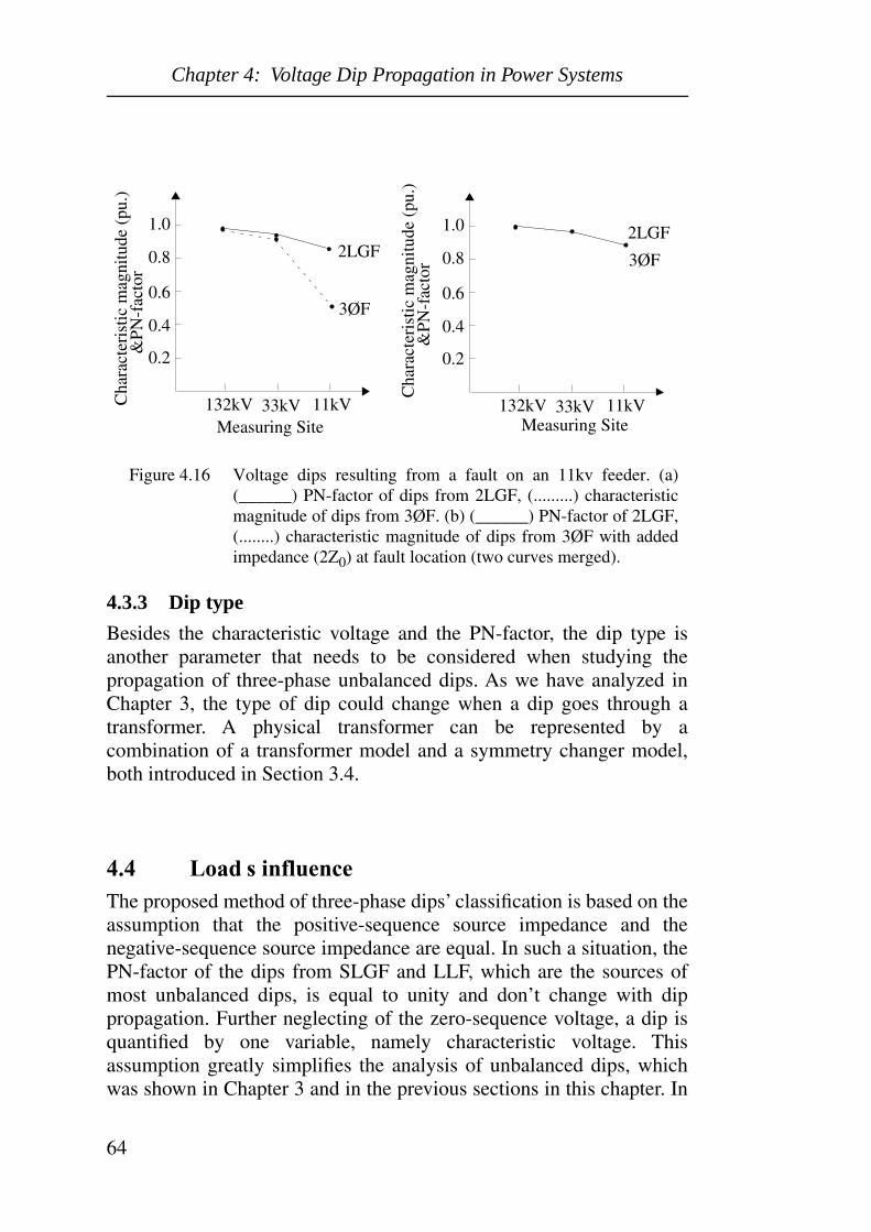
Chapter 4: Voltage Dip Propagation in Power Systems
64
4.3.3 Dip type
Besides the characteristic voltage and the PN-factor, the dip type isanother parameter that needs to be considered when studying thepropagation of three-phase unbalanced dips. As we have analyzed inChapter 3, the type of dip could change when a dip goes through atransformer. A physical transformer can be represented by acombination of a transformer model and a symmetry changer model,both introduced in Section 3.4.
4.4 Load s influenceThe proposed method of three-phase dips’ classification is based on theassumption that the positive-sequence source impedance and thenegative-sequence source impedance are equal. In such a situation, thePN-factor of the dips from SLGF and LLF, which are the sources ofmost unbalanced dips, is equal to unity and don’t change with dippropagation. Further neglecting of the zero-sequence voltage, a dip isquantified by one variable, namely characteristic voltage. Thisassumption greatly simplifies the analysis of unbalanced dips, whichwas shown in Chapter 3 and in the previous sections in this chapter. In
Figure 4.16 Voltage dips resulting from a fault on an 11kv feeder. (a)(______) PN-factor of dips from 2LGF, (.........) characteristicmagnitude of dips from 3ØF. (b) (______) PN-factor of 2LGF,(........) characteristic magnitude of dips from 3ØF with addedimpedance (2Z0) at fault location (two curves merged).
132kV 33kV 11kV
1.0
0.8
0.6
0.4
0.2
132kV 33kV 11kV
1.0
0.8
0.6
0.4
0.2
Cha
ract
eris
tic m
agni
tude
(pu
.)
Measuring Site Measuring Site
&PN
-fac
tor
Cha
ract
eris
tic m
agni
tude
(pu
.)&
PN-f
acto
r
2LGF
3ØF
2LGF
3ØF

Chapter 4: Voltage Dip Propagation in Power Systems
65
a system with large induction motor loads connected, however, theerror of this assumption increases. In the simulations performed inSection 4.1 and 4.2, we assumed static loads for all the situations. Inreality, dynamic loads, such as induction motors, can not berepresented as a constant impedance. The dynamic loads influence thedip characteristics in two ways. The first effect is that a dip becomesnon-rectangular. That is, a dip takes one or two cycles to reach thebottom and recovers gradually after the system fault is cleared, whichis known as the post-fault dip. The second effect is for unbalanced dips,where a non-unity PN-factor often results.
4.4.1 Motor re-acceleration
In a static system with only constant-impedance load, a rectangular dipcan be assumed. That is, the calculation of magnitude and duration of adip can be based on two simple assumptions:
1) Due to the short circuit, the voltage drops to a low valueimmediately.
2) When the fault is cleared, the voltage recovers immediately.
These assumptions, however, do not hold in the case of a substantialpart of the load consisting of electrical motors like in many industrialpower systems. The motors decelerate during the short circuit. Afterfault-clearing they will accelerate again, drawing high current from thesupply, causing a post-fault voltage dip. A measured dip with a longpost-fault component is shown in Figure 4.17. Such a post-fault dipprolongs the dip duration. Certain equipment which survived at theduring-fault dip may trip at this stage. In defining the voltage dipshape, the assumption of a rectangular dip no longer holds in case oflarge induction motor loads. Taking motor behavior into account willmake it no longer possible to define a dip simply by its duration andmagnitude.

Chapter 4: Voltage Dip Propagation in Power Systems
66
A method of characterisation of non-rectangular voltage dips ispresented in [36]. The concept is to split the dip into two parts, theduring-fault dip and the post-fault dip. For the during-fault part, arectangular dip is assumed, where the deepest point is considered asthe magnitude of during-fault dip and the fault clearing time isconsidered as the duration of the during-fault dip. For the post-faultpart, the point where the voltage recovers is considered as the post-fault dip magnitude, and the period during which the voltage is below acertain level (e.g. 90%) is considered as the post-fault duration. Thecorresponding contour chart for non-rectangular dip is developed in[39].
4.4.2 PN-factor
In the case of positive- and negative-sequence source impedance aredifferent, the two-component method for symmetrical componentscan’t be used. The PN- factor as defined in Chapter 3 will no longer beequal to unity for SLGF and LLF. The following equations giveexpressions for the PN-factor based on a three-component symmetricalcomponent analysis.
SLGF
(4.2)
0 0.05 0.1 0.15 0.2 0.25 0.3 0.35-1.5
-1
-0.5
0
0.5
1
1.5
Time [s]
Vol
tage
[pu
.]
Figure 4.17 Measured dip with a clear post-fault component, data obtainedfrom scottish power.
F 1Zs2 Zs1–
Zs0 Zs1 Zs2+ +( ) Zf0 Zf1 Zf2+ +( )+----------------------------------------------------------------------------------------------+=

Chapter 4: Voltage Dip Propagation in Power Systems
67
LLF
(4.3)
Equations (4.2) and (4.3) show that in case of unequal positive- andnegative-sequence source impedances, the PN-factors of dips due toSLGF and LLF are no longer equal to unity.
Induction machines are the main reason that positive- and negative-sequence source impedances are not equal. The induction motor isusually represented by a “transformer equivalent”, i.e., a T equivalentwhere separate series branches represent the stator (primary) circuitand the rotor (secondary) circuit, with a shunt branch to represent ironlosses and excitation. At standstill or locked rotor the inductionmachine is indeed a transformer. With the motor turning, however, theequivalent impedance of the secondary or rotor circuit is seen to be afunction of the slip s as noted in Figure 4.18.
If negative-sequence voltages are applied to the induction motor, arevolving flux wave is established in the machine air gap which isrotating backwards. Then the slip of the rotor with respect to thenegative-sequence field is 2-s. The equivalent circuit for negative-sequence is the same as that of Figure 4.18 with s replaced by 2-s asshown in Figure 4.19.
F 1Zs2 Zs1–
Zs1 Zs2+( ) Zf1 Zf2+( )+---------------------------------------------------------------+=
Rs
Er1
Xs
Rrs
------
Xr
Xm
Is1Ir1
Va1
Figure 4.18 Positive-sequence induction motor equivalent circuit
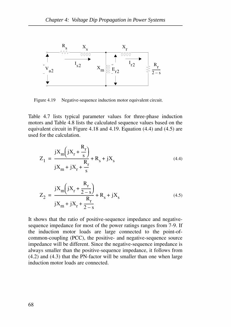
Chapter 4: Voltage Dip Propagation in Power Systems
68
Table 4.7 lists typical parameter values for three-phase inductionmotors and Table 4.8 lists the calculated sequence values based on theequivalent circuit in Figure 4.18 and 4.19. Equation (4.4) and (4.5) areused for the calculation.
(4.4)
(4.5)
It shows that the ratio of positive-sequence impedance and negative-sequence impedance for most of the power ratings ranges from 7-9. Ifthe induction motor loads are large connected to the point-of-common-coupling (PCC), the positive- and negative-sequence sourceimpedance will be different. Since the negative-sequence impedance isalways smaller than the positive-sequence impedance, it follows from(4.2) and (4.3) that the PN-factor will be smaller than one when largeinduction motor loads are connected.
Rs
Er2
Xs
Rr2 s–-----------
Xr
Xm
Is2Ir2
Va2
Figure 4.19 Negative-sequence induction motor equivalent circuit.
Z1
jXm jXr
Rrs
-----+
jXm jXr
Rrs
-----+ +
-------------------------------------- Rs jXs+ +=
Z2
jXm jXr
Rr2 s–-----------+
jXm jXr
Rr2 s–-----------+ +
-------------------------------------------- Rs jXs+ +=

Chapter 4: Voltage Dip Propagation in Power Systems
69
Table 4.7: Approximate Constants for Three-Phase Induction Motors
source: P.Andersson [12].
Table 4.8: Calculated Sequence Values for Three-Phase Induction Motors
To look at the influence of induction motor loads on dip characteristicsquantitatively, we simulated SLGF in the simple network shown inFigure 4.20.
Rating
(HP)
Full load slip (%)
R and X in per Unit*
Xs Xr Xm Rs Rr
Up to 5 3.0-5.0 0.05-0.07 0.05-0.07 1.6-2.2 0.04-0.06 0.04-0.06
5-25 2.5-4.0 0.06-0.08 0.06-0.08 2.0-2.8 0.035-0.05 0.035-0.05
25-200 2.0-3.0 0.075-0.085 0.075-0.085 2.2-3.2 0.03-0.04 0.030-0.04
200-1000 1.5-2.5 0.075-0.085 0.075-0.085 2.4-3.6 0.025-0.03 0.020-0.03
over 1000
1.0 0.075-0.085 0.075-0.085 2.6-4.0 0.015-0.02 0.015-0.025
Rating
(HP)
R and X in per Unit* |Z1/Z2|
R1 X1 R2 X2
Up to 5 0.80-0.94 0.71-0.60 0.06-0.09 0.10-0.14 9.3-6.8
5-25 0.94-1.04 0.73-0.59 0.05-0.07 0.12-0.16 9.2-6.9
25-200 1.0-1.13 0.79-0.61 0.04-0.06 0.15-0.17 8.3-7.2
200-1000 1.0-1.07 0.67-0.51 0.03-0.04 0.15-0.17 7.9-6.8
over 1000 1.09-1.76 0.75-1.24 0.02-0.03 0.15-0.17 8.9-12.6
InductionMotor
ImpedanceLoad
2 km
SLGF
13.8 kV
PowerSource
Figure 4.20 A simple 13.8 kV network.
E
Zf
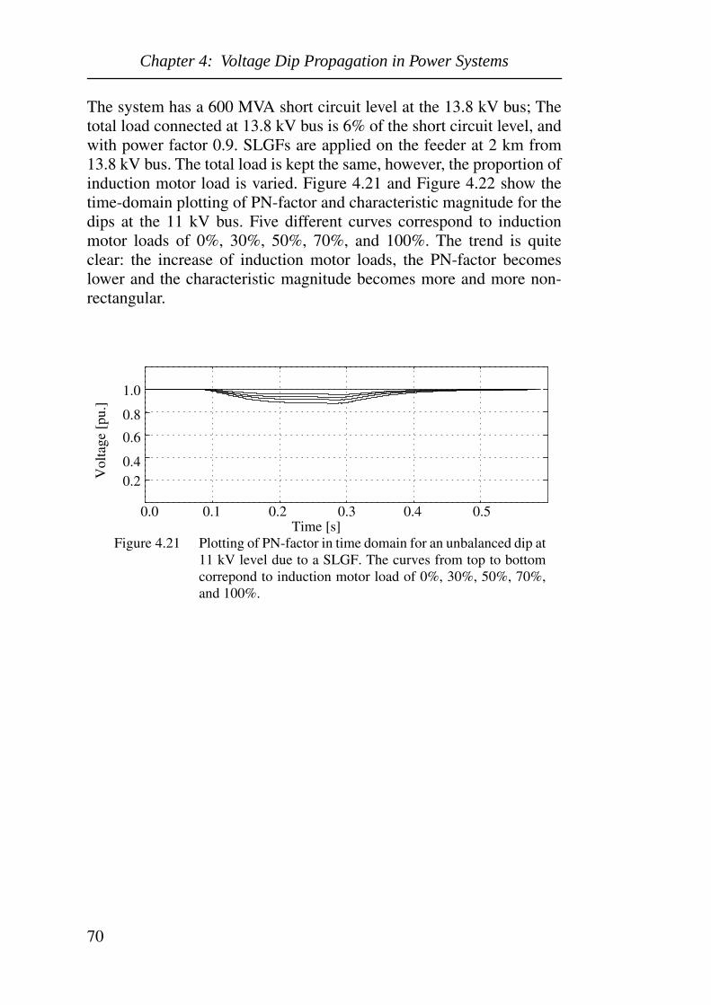
Chapter 4: Voltage Dip Propagation in Power Systems
70
The system has a 600 MVA short circuit level at the 13.8 kV bus; Thetotal load connected at 13.8 kV bus is 6% of the short circuit level, andwith power factor 0.9. SLGFs are applied on the feeder at 2 km from13.8 kV bus. The total load is kept the same, however, the proportion ofinduction motor load is varied. Figure 4.21 and Figure 4.22 show thetime-domain plotting of PN-factor and characteristic magnitude for thedips at the 11 kV bus. Five different curves correspond to inductionmotor loads of 0%, 30%, 50%, 70%, and 100%. The trend is quiteclear: the increase of induction motor loads, the PN-factor becomeslower and the characteristic magnitude becomes more and more non-rectangular.
Time [s]
Vol
tage
[pu
.]
Figure 4.21 Plotting of PN-factor in time domain for an unbalanced dip at11 kV level due to a SLGF. The curves from top to bottomcorrepond to induction motor load of 0%, 30%, 50%, 70%,and 100%.
0.20.4
0.6
0.8
1.0
0.0 0.1 0.2 0.3 0.4 0.5

Chapter 4: Voltage Dip Propagation in Power Systems
71
The simulation is performed with constant load but various proportionsof induction motor load. But this doesn’t mean PN-factor only dependson the ratio between impedance load and induction load. An increaseof induction motor load always results in lower PN-factor.
Besides the inequality of positive- and negative- sequence sourceimpedances, the induction motor loads also have another effect on thePN-factor. The positive-sequence impedance of the induction motordecreases gradually during the dip [21]. This effect also contributes toa lower PN-factor. The left column of Figure 4.24 shows the sequencenetworks of the system in Figure 4.20, where Zs1, Zs2, Zs0 aresequence impedances of the “power source”; Zl1, Zl2, Zl0 are sequenceimpedances of the total load (“impedance” + “induction motor”); Zf1,Zf2, Zf0 are sequence impedances of the feeder between the 13.8 kVbus and the fault location.
0.0 0.1 0.2 0.3 0.4 0.5
Time [s]
Vol
tage
[pu
.]
0.20.4
0.6
0.8
Figure 4.22 Plotting of characteristic magnitude in time domain for anunbalanced dip at 11 kV level. The curve from rectangular tonon-rectangular correspond to induction motor load of 0%,30%, 50%, 70%, and 100%.
1.0

Chapter 4: Voltage Dip Propagation in Power Systems
72
Note the difference with the voltage divider model shown in Section3.1 in Chapter 3. The load is explicitly included in the circuit. Thestandard voltage divider model show in the right column of Figure 4.24is obtained by the following,
(4.6)
(4.7)
(4.8)
(4.9)
Previously, the analysis was based on E´ = 1. Load was implicitlyincluded, but the load was not supposed to change impedance duringthe event.
E
Zs1
Zl1
Zf1
Zs2 Zf2
Zl2
Zl0
Zs0 Zf0
PCC
PCC
PCC
Figure 4.24 The sequence network of the system in Figure 4.20.
E´
Z´s1 Zf1
Z´s2 Zf2
Z´s0 Zf0
PCC
PCC
PCC
Load model non-load model
E′
EZl1
Zl1 Zs1+-----------------------=
Zs1′ Zs1Zl1
Zs1 Zl1+-----------------------=
Zs2′ Zs2Zl2
Zs2 Zl2+-----------------------=
Zs0′ Zs0Zl0
Zs0 Zl0+-----------------------=
Chapter 4: Voltage Dip Propagation in Power Systems
73
With the speed of the motor slows down during the dip, the slip sincreases. From the equivalent circuit of positive- and negative-sequence impedance of induction motor loads shown in Figure 4.18and 4.19, it can be concluded that the slip influences the sequenceimpedance. Thus, the positive-sequence impedance decreases but thenegative-sequence impedance remains constant. The zero-sequenceimpedance of the induction motors is infinite, thus Z´s0 is not affectedby the increased slip either. As Equation (4.6) shows, the decreasedpositive-sequence impedance results in a decreased voltage E´.Physically, we can also understand this effect as another “simultaneous3ØF fault” due to the rather high power consumption because of theincreased slip of the induction motor.
4.4.3 Limitations of the classification method
The proposed classification theory of three-phase voltage dips and thefollowing theory of their propagations are based on the assumption thatthe positive- and negative- sequence source impedances are equal.Loads are of constant-impedance type with equal positive- andnegative-sequence impedances. The benefit of this simplification is inthat it offers an analytical single-phase method for voltage dip studieseven in unbalanced cases. Thus, the theory developed for three-phasebalanced dips can be extended to unbalanced dips with only slightmodification. However, in the case of large induction motor loadspresent in the system, the error may increase to such a level that it isnot suitable to use this theory. In this case, we have to turn totraditional symmetrical components or digital simulations.

Chapter 4: Voltage Dip Propagation in Power Systems
74

Chapter 5: Field Measurement Analysis
75
Chapter 5 Field Measurement Analysis
Power quality surveys play important roles in defining the electricalenvironment. Efforts have been made in several nations resulting inlarge quantities of survey data. IEEE std 1159 [8] gives practicalinstructions for monitoring electric power quality and interpreting theresults. However, voltage dips are only generally described in thedocument, where it is characterized by magnitude and duration only.Some other aspects of voltage dip characteristics, such as phase-angleshift, point-on-wave, and three-phase unbalance are not included. Morerecent publications have introduced different ways in presentingvoltage dips and other voltage variations from power quality surveys[30][31][32]. This chapter intends to apply the theory of dipclassification to present measured voltage dips. The measuring data areobtained from different sources [29][33]. The measuring sites rangefrom low voltage level (230 V), to distribution systems (11kV, 33kV,132kV), and transmission systems (220kV, 400 kV).
5.1 Obtaining dip characteristics Based on the dip classification theory proposed in Chapter 3, a three-phase voltage dip can be fully characterized by four values: dip type,characteristic voltage, PN-Factor (only for unbalanced dips), and zero-sequence (only for unbalanced dips). Knowing the four characteristics,three phase voltages of a dip can be reproduced. Note that dip typescan reach three values (A, C, D), where the other three characteristicsare complex values (6 real values). To fully characterize the dip, wethus need 7 real values. The advantage of using this characterization topresent voltage dip is that the resulting characteristics can be furtherreduced, since PN-factor is normally close to one and zero-sequencevoltage can be assumed zero. Thus, a three-phase voltage dip can becharacterized by one variable, namely characteristic voltage, and itstype. Also, the argument of the characteristic voltage may be neglectedfor some applications, so that only the dip type and one real valueremains.
5.1.1 Principle
To obtain the characteristics from recorded voltage waveshapes, theequations listed in Table 3.2 are used as the mathematical base. FromTable 3.2, it follows that the positive-sequence voltage is always along

Chapter 5: Field Measurement Analysis
76
the reference phase axis. The direction of the negative-sequencevoltage depends on the type of dip. For type Ca the negative-sequencevoltage is along the positive real axis; for type Cb the negative-sequence voltage is leading by 1200; for type Dc by 600, etc. Byrotating the negative-sequence voltage over an integer multiple of 600
all dip types can be obtained from one prototype dip; dip type Ca hasbeen chosen as the prototype dip. From Table 3.2, the followingrelationship between positive- and negative- sequence voltage isobtained for the prototype dip:
(5.1)
The dip type may be obtained from the angle between the negative-sequence voltage of the measured dip and the negative-sequencevoltage of the prototype. Due to various approximations made andmeasurement errors, this angle is not exactly an integer multiple of 600
so that the following expression may be used to obtain the dip type:
(5.2)
k = 0 type Cak = 1 type Dck = 2 type Cbk = 3 type Dak = 4 type Cck = 5 type Db
Knowing the dip type, the negative-sequence voltage can be calculatedback to the corresponding value for the prototype dip:
(5.3)
where k is obtained according to (5.2) and V2 the negative-sequencevoltage of the measured dip. Characteristic voltage V and PN-factor Fare obtained from the expressions for the prototype dip:
(5.4)
V2 ref, 1 V1–=
k roundangle V2 1 V1–,( )
600
---------------------------------------------
=
V2′
V2ejk60
0–
=
V V1 V2′
–=
F V1 V2′
+=

Chapter 5: Field Measurement Analysis
77
This method has been applied to data obtained from various sources.From the recorded voltage waveforms, positive- and negative-sequencevoltages are calculated. To obtain the dip type, the angle is obtainedbetween V2 and 1-V1. In Figure 5.1 the negative-sequence voltage V2is plotted against the “drop in positive-sequence voltage” 1- V1. Thelatter is toward the right in the figure, so that the direction of each pointgives the angle between V2 and 1-V1. The distance between each pointand the origin corresponds to the absolute value of the negative-sequence voltage.
Figure 5.1 shows the scatter plot of the measured unbalanced dips fromvarious sources. Each dot represent the negative-sequence voltage V2of a measured dip compared to 1-V1. When the PN-factor F exactlyequals 1, the scatter dots will all fall on one of the six axes in the figure.Due to non-unity PN-factor, the dots are spread around these axes, butin almost all cases, the dots are close to one of the six axes. Anexception is some dots close to the origin of the diagram. These dotsrepresent shallow dips, where a small error may change the apparentdip type. We assume that the dots distributed within -300 and +300
region from an axis have the same dip type as the dots falling on theaxis. Equation (5.2) expresses this principle in a mathematical way.
The measuring data presented in Figure 5.1 shows that,
Figure 5.1 Recognition of dip types, data obtained from Scottish Power,SINTEF, and STRI.
Cb Dc
Da
DbCc
Ca(1-V1)

Chapter 5: Field Measurement Analysis
78
1. Most dots are close to the origin. Those dots represent shallow dips,which have small negative-sequence voltages. The shallow dips are themajority of the measurements.
2. The dots within each region appears shifted toward the right sidecompared to the “ideal case”. This phenomenon is due to thecharacteristics of the PN-factor. As will be shown later (Figure 5.9 andFigure 5.11), PN-factor values measured are slightly less than one inabsolute value with a negative argument. In a certain system, it may bepossible to use an PN-factor other than 1.0 to obtain V´2, so that thedots will distribute around the “average case”.
5.1.2 Algorithms for dip characterization
The proposed algorithm for classification and characterization of three-phase unbalanced dips consists of a number of steps. It is assumed thattime-domain sampled data are available for all the three phasesincluding at least two cycles of pre-event voltages.
1. Determine the voltage frequency from the pre-event voltagesamples.
2. Determine voltage phasors for the three phase voltages by using aDFT (Discrete Fourier Transform) algorithm. The voltage frequency isused to obtain the phase-angle shift between the during-event and thepre-event voltage.
3. Calculate positive-, negative-, and zero-sequence voltages by usingexpression (3.9).
4. Determine if the dip is balanced or unbalanced from the magnitudeof the negative-sequence voltage V2 compared to the positive-sequencevoltage V1. If |V2| << |1- V1| the dip is balanced.
5. For balanced dips the dip type is A and the characteristic voltageequals the positive-sequence voltage.
6. For unbalanced dips the dip type is determined from positive- andnegative-sequence voltages by using expression (5.2). Thecharacteristic voltage V and PN-factor F are obtained by usingexpression (5.4).
7. A balanced dip is fully characterized through the characteristicvoltage V.

Chapter 5: Field Measurement Analysis
79
8. An unbalanced dip is fully characterized through the dip type,characteristic voltage, PN-factor and zero-sequence voltage.
5.1.3 Examples
Two examples of three-phase unbalanced dips obtained frommeasurements are shown in Figure 5.2 and Figure 5.3. Due to the dipin Figure 5.2, the equipment will experience a drop in voltage for onephase, where the dip in Figure 5.3 will lead to a drop in two phases.The effect of these two events on the equipment is likely to bedifferent, but they would be characterized as identical events if only thelowest phase magnitude and duration are used for characterization.
0.05 0.1 0.15 0.2 0.25 0.3 0.35-1.5
-0.5
0.5
1.5
Vol
tage
[pu
.]
Time [s]
Figure 5.2 An example of a three-phase unbalanced dip with one phaseexperiencing a severe drop in voltage (waveform I).

Chapter 5: Field Measurement Analysis
80
The proposed characterization method has been applied to the three-phase unbalanced dips shown in Figure 5.2 and Figure 5.3. Followingthe algorithm described in Section 5.1.2, we obtain the characterizationresults:
A. Following step 1, the voltage frequency of each event is obtainedfrom the pre-event voltage samples. The results are: Waveform I:49.994 Hz, waveform II: 50.073 Hz. These values are used as thefundamental frequency in performing DFT analysis.
B. Following step 2 and step 3, the voltage phasors are obtained byDFT, and the symmetrical components are calculated. Thecharacteristic values and phasor diagram for waveform I are shown inFigure 5.4 and Table 5.1. The results for waveform II are shown inFigure 5.5 and Table 5.2. The phasors of the dips are obtained on thesecond cycle of the waveform after the dip initiation.
0.05 0.1 0.15 0.2 0.25 0.3 0.35-1.5
-0.5
0.5
1.5
Time [s]
Vol
tage
[pu
.]
Figure 5.3 An example of a three-phase unbalanced dip with two phasesexperiencing severe drops in voltage (waveform II).

Chapter 5: Field Measurement Analysis
81
Table 5.1: Characteristics of waveform I
Dip Type
Characteristic voltage (V)
PN-factor (F)
Zero-sequence
(V0)
Positive-sequence
(V1)
Negative-sequence
(V2)
Drop in positive-sequence
(1-V1)
Dc 0.76∠-10 0.98∠-00 0.06∠-55.80 0.87∠-10 0.12∠600 0.13∠6.70
Figure 5.4 Waveform I (a) Three-phase phasor diagram; (b) Sequencephasor diagram;
(a) (b)
a
b
c
Va
Vb
Vc
a
c
b
V1V2
Figure 5.5 Waveform II (a) Three phase phasor diagram; (b) Sequencephasor diagram;
a
b
c
Va
Vc
Vb
a
b
c
V1
V2
(a)(b)

Chapter 5: Field Measurement Analysis
82
Table 5.2:Characteristics of Waveform II
C. By using (5.1) and (5.2) (step 4 and step 5), the dip types aredetermined.
For waveform I we obtained
V2 = 0.12∠600, V1 = 0.87∠-10, 1-V1 = 0.13∠6.70
The angle between V2 and (1-V1) is 53.30, which according to (5.2)gives a dip of type Dc. Note that type Dc is a major drop in phase Cwith minor drops in phases a and b. After rotating the negative-sequence voltage over -600, according to (5.3), we obtain
V1 = 0.87∠-10 and V2´= 0.12∠00
Applying (5.4) gives the characteristic voltage
V = V1- V2´= 0.76∠-10
and the PN-factor
F = V1 + V2´= 0.98∠-00
For waveform II the angle between V2 and 1-V1 is equal to 1110,resulting in dip type Cb (a major drop in phases a and c), the PN-factorF = 0.98∠-20 and the characteristic voltage V = 0.56∠-40.
D. By using (5.4), the characteristic voltage V and PN-factor F arecalculated, as shown in Table 5.1 and 5.2. Note that the characteristicmagnitude of waveform II is much less (56%) than of waveform I(76%) despite them having the same “lowest phase voltage”.
The characteristic magnitude and PN-factor can also be plotted as afunction of time, shown in Figure 5.6 and Figure 5.7. Thecharacteristics are obtained from a one-cycle “moving window”.
Several observations can be made from these figures:
Dip Type
Characteristic voltage (V)
PN-factor (F)
Zero-sequence
(V0)
Positive-sequence
(V1)
Negative-sequence
(V2)
Drop in positive-sequence
(1-V1)
Cb 0.56∠-40 0.98∠-20 0 0.77∠-30 0.21∠1210 0.23∠9.90

Chapter 5: Field Measurement Analysis
83
1. Neither the characteristic voltage V nor the PN-factor F iscompletely constant during the dip, both show small and slowdecreases. This shows the contribution from dynamic loads. Theinfluence from dynamic loads on dip characteristics is discussed inSection 4.4.
2. After fault-clearing (i.e. after the main recovery in voltage), bothcharacteristic voltage V and PN-factor F still show a small drop withslow recovery to their pre-event values (1.0 pu.). This is most clearlyvisible in Figure 5.7. The post-fault dip is balanced so thatcharacteristic voltage V and PN-factor F are equal. An explanation forthis phenomenon is given in Section 4.4.
0.05 0.1 0.15 0.2 0.25 0.3
0.2
0.4
0.6
0.8
1.0
Time [s]
Vol
tage
[pu
.]
Figure 5.6 Characteristic magnitude (lower curve) and PN-factor (uppercurve) as a function of time, for waveform I.
0.35

Chapter 5: Field Measurement Analysis
84
5.2 Characteristics obtained from measurementsAs we have mentioned in Section 3.3.5, the accuracy of the theory ofdip classification depends on the correctness of several assumptions.The assumption that the positive- and negative-sequence sourceimpedance are equal is most critical. From this assumption, it followsthat the PN-factor of an unbalanced dip is equal to unity and constantas the dip propagates in the power system. To verify the theory, wehave collected measurement data from several data sources. Followingthe algorithm introduced in Section 5.1, the characteristic values areobtained. The phasor values are obtained by DFT phasor detection onthe second cycle of each dip after the dip initiation.
5.2.1 Transmission system: Sweden
The Swedish Transmission Research Institute (STRI) performed powerquality measurements in the swedish transmission system at four400/220 kV substations from March 1996 to November 1996. Fromthe measured dip data, the characteristic voltages and PN-factors of thedips are obtained and presented as scatter plots in the “magnitude-phase-angle plane”. Figure 5.9 shows the characteristic voltage and thePN-factor of unbalanced dips, namely type C and type D, and Figure5.10 shows the characteristic voltage of balanced dips, namely type A.
0.05 0.1 0.15 0.2 0.25 0.3
0.2
0.4
0.6
0.8
1
Time [s]
Vol
tage
[pu
.]
Figure 5.7 Characteristic magnitude (lower curve) and PN-factor (uppercurve) as a function of time, for waveform II.
0.35

Chapter 5: Field Measurement Analysis
85
Figure 5.9 shows that the PN-factors of unbalanced dips intransmission systems are close to 1. The reason is that the dynamic
0.2 0.4 0.6 0.8 1.0-40
-30
-20
-10
0
10
20
30
40
Magnitude (pu.)
Arg
umen
t (de
gree
)
Figure 5.9 Scatter plots of PN-factors and characteristics voltage ofunbalanced dips in “argument - magnitude plane”, data obtainedfrom STRI (Dot -- PN-factor, Star -- characteristic voltage).
0.2 0.4 0.6 0.8 1.0-40
-30
-20
-10
0
10
20
30
40
Magnitude (pu.)
Arg
umen
t (de
gree
)
Figure 5.10 Scatter plots of characteristic voltages of balanced dips in“argument - magnitude plane”, data obtained from STRI.

Chapter 5: Field Measurement Analysis
86
loads are far from the transmission system, thus the positive- andnegative- sequence source impedance are equal. Two dots withsomewhat smaller PN-factors may indicate dips resulted from 2LGF. Italso shows that the arguments of the characteristic voltage for bothbalanced and unbalanced dips are quite small. As explained in Chapter3 and Chapter 4, the argument of the characteristic voltage is due to theX/R ratio difference of the source and feeder. Since there is no clearseparation of source and feeder in transmission systems, it is consistentwith the theory that the argument is small.
5.2.2 Distribution system: Scotland
Scottish Power implemented an extensive monitoring program to helpidentify quality of supply characteristics at a number of sites on itssystem. The utility has used the collected data to identify where powersystem performance can be improved and where customers canimprove the immunity of their processes to voltage dips. We obtainedfrom Scottish Power some measured voltage dips to apply theproposed classification. The data are mostly from distribution systems(132 kV, 33kV, 11kV). Figure 5.11 shows the characteristic voltagesand PN-factors for unbalanced dips. Figure 5.12 shows thecharacteristic voltages for balanced voltage dips.
0.2 0.4 0.6 0.8 1.0-40
-30
-20
-10
0
10
20
30
40
Arg
umen
t (de
gree
)
Magnitude (pu.)
Figure 5.11 Scatter plots of PN-factors and characteristics voltages ofunbalanced dips in “argument - magnitude plane”, dataobtained from Scottish Power (Dot -- PN-factor, Star --Characteristic voltage).

Chapter 5: Field Measurement Analysis
87
The following observations are made from the measurements:
1. The PN-factors of most measured dips are close to 1 in distributionsystems with a few exceptions. The waveforms of those dips withlower PN-factors also show long post-fault dips, which indicates thepresence of induction motor loads. Voltage dip propagation influencedby induction motor loads, will be shown in Section 5.3.
2.The arguments of the characteristic voltage of both balanced andunbalanced dips are mostly negative. This is due to the source having abigger X/R ratio than the feeders in distribution systems.
3. Several bigger argument of the characteristic voltage of balanceddips are observed. This could be due to two reasons: 1) Mostunbalanced dips are caused by SLGF, where the argument ofcharacteristic voltage is smaller. 2)Balanced dips are often caused bycable fault. The X/R ratio of cable is much smaller than the X/R ratioof the source.
5.2.3 Distribution system: Norway
The Norwegian Electric Power Research Institute (SINTEF) hasmeasured voltage dips and other voltage disturbances at over 400 sitesin Norway during November 1992 to June 1996 [29]. Most of thesesites are at 230 V level with a few at 6 kV and 11 kV. The measuring
0.2 0.4 0.6 0.8 1.0-40
-30
-20
-10
0
10
20
30
40
Arg
umen
t (de
gree
)
Magnitude (pu.)
Figure 5.12 Scatter plot of characteristic voltages of balanced dips in“argument - magnitude plane”, data obtained from ScottishPower (Star -- Characteristic voltage).

Chapter 5: Field Measurement Analysis
88
period for each site varies from several weeks to a few months. Figure5.13 shows the characteristic voltages and PN-factors for unbalanceddips. Figure 5.14 shows the characteristic voltages for balanced voltagedips.
0.2 0.4 0.6 0.8 1.0-40
-30
-20
-10
0
10
20
30
40
Figure 5.13 Scatter plots of PN-factor and characteristic voltage ofunbalanced dips in “argument - magnitude plane”, dataobtained from SINTEF (Dot -- PN-factor, Star -- Characteristicvoltage).
Arg
umen
t (de
gree
)
Magnitude (pu.)

Chapter 5: Field Measurement Analysis
89
The PN-factors of most measured unbalanced dips from themeasurements are also quite close to 1 (98% in average) in distributionsystems. However, the arguments of characteristic voltages are rathersmall and distributed around zero, contrary to the results shown inFigure 5.11 and 5.12. Two possible explanations are:
1. The measured dips are rather shallow;2. The difference of X/R ratio between the source and feeders is
small.
Analysis of measured dips, both in transmission and distributionsystems, shows that the PN-factor is close to unity. This indicates thatthe assumption, namely positive- and negative- source impedance areequal, generally holds in distribution systems and transmissionsystems.
0.2 0.4 0.6 0.8 1.0-40
-30
-20
-10
0
10
20
30
40
Arg
umen
t (de
gree
)
Magnitude (pu.)Figure 5.14 Scatter plots of characteristic voltage of balanced dips in
“argument - magnitude plane”, data obtained from SINTEF(Star -- Characteristic voltage).
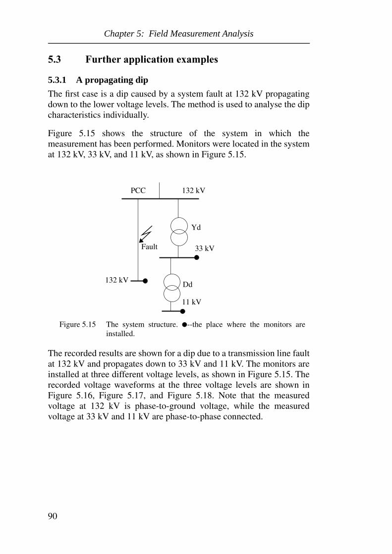
Chapter 5: Field Measurement Analysis
90
5.3 Further application examples
5.3.1 A propagating dip
The first case is a dip caused by a system fault at 132 kV propagatingdown to the lower voltage levels. The method is used to analyse the dipcharacteristics individually.
Figure 5.15 shows the structure of the system in which themeasurement has been performed. Monitors were located in the systemat 132 kV, 33 kV, and 11 kV, as shown in Figure 5.15.
The recorded results are shown for a dip due to a transmission line faultat 132 kV and propagates down to 33 kV and 11 kV. The monitors areinstalled at three different voltage levels, as shown in Figure 5.15. Therecorded voltage waveforms at the three voltage levels are shown inFigure 5.16, Figure 5.17, and Figure 5.18. Note that the measuredvoltage at 132 kV is phase-to-ground voltage, while the measuredvoltage at 33 kV and 11 kV are phase-to-phase connected.
Fault
132 kV
33 kV
11 kV
PCC
Figure 5.15 The system structure. --the place where the monitors areinstalled.
Yd
Dd132 kV

Chapter 5: Field Measurement Analysis
91
The waveforms shows that a SLGF occurs on phase a of the 132 kVtransmission line. This results in a type Da dip on the 132 kV bus. The
0.0 0.05 0.1 0.15 0.2 0.25 0.3-1.5
-0.5
0.5
1.5
Time (s)
Vol
tage
(pu
)
Figure 5.16 Voltage waveform at 132 kV.
0.0 0.05 0.1 0.15 0.2 0.25 0.3-1.5
-0.5
0.5
1.5
Time (s)
Vol
tage
(pu
)
Figure 5.17 Voltage waveform at 33 kV.
0.0 0.05 0.1 0.15 0.2 0.25-1.5
-0.5
0.5
1.5
Vol
tage
(pu
)
Time (seconds)
0.3
Figure 5.18 Voltage waveform at 11 kV.

Chapter 5: Field Measurement Analysis
92
faulted line is disconnected after 4 cycles. The monitoring equipment isinstalled at the line side of the circuit breaker, so it also captures thedecreasing voltage waveform after the faulted line is cleared. The first4 cycles of the dip propagate down to low voltage level, which resultsin a Db type dip at 33 kV and a Cc type dip at 11 kV.
Following the method introduced in Section 5.1, the characteristics ofthe measured dips are obtained for the second cycle after dip initiation.Figure 5.19, Figure 5.20, and Figure 5.21 show the three-phase phasordiagram and the sequence phasor diagram. Table 5.3, Table 5.4, andTable 5.5 show the calculated characteristic values of the measureddips.
Table 5.3: Characteristics of dip at 132 kV
Type Characteristic voltage (V)
PN-factor (F)
Zero-sequence
(V0)
Positive-sequence
(V1)
Negative-sequence
(V2)
Da 0.31∠-110 0.98∠-20 0.14∠-1670 0.64∠-40 0.34∠-1780
a
c
a
c
b b
Figure 5.19 132 kV (a) Three-phase phasor diagram; (b) Sequence phasordiagram;
Va
Vb
Vc
V1
V2
V0
(a) (b)

Chapter 5: Field Measurement Analysis
93
Table 5.4: Characteristics of dip at 33 kV
Table 5.5:Characteristics of dip at 11 kV
Type Characteristic voltage (V)
PN-factor (F)
Zero-sequence
(V0)
Positive-sequence
(V1)
Negative-sequence
(V2)
Db 0.40∠-110 0.95∠-30 0 0.68∠-60 0.28∠-580
Type Characteristic voltage (V)
PN-factor (F)
Zero-sequence
(V0)
Positive-sequence
(V1)
Negative-sequence
(V2)
Cc 0.54∠-80 0.93∠-50 0 0.74∠-60 0.20∠-1200
a a
b b
c c
(a) (b)
VaVb
Vc
V1V2
Figure 5.20 33 kV (a) Three phase phasor diagram; (b) Sequence phasordiagram;
a a
b b
c c
(a) (b)
VaVb
Vc
V1V2
Figure 5.21 11 kV (a) Three-phase phasor diagram; (b) Sequence phasordiagram;

Chapter 5: Field Measurement Analysis
94
Several things can be observed from this propagating dip by using theproposed characterization:
1.There is a type 1 transformer (Yd) with a type 1 symmetry changer (ato b) between 132 kV and 33 kV, which changes the Da dip to a Cb dip.However, the phase-to-phase connected monitor measurde a dip oftype Db instead. A type 1 transformer (Dy) with a type 1 symmetrychanger (b to c) between 33 kV and 11 kV changes the Cb dip to a Dcdip, but the phase-to-phase connected monitor measured a Cc dipinstead. This phenomena shows that, in recognizing dip type frommeasurement from field measurement, it is important to consider themonitor’s connection.
2. The zero-sequence voltage is removed from the dip at 33 kV becauseof the transformer.
3. An increased characteristic magnitude is observed when the dippropagates from 132 kV down to 33 kV and 11 kV (31%, 40%, and54%). This phenomena has also been observed with other measuredpropagating dips. It is hard to give a clear explanation without detailedinvestigation. However, several possible reasons could be:1)Embedded generation; 2) Reduction of loads during dips, e.g. trip ofrectifier loads; 3) Induction motor loads feeding to the fault due to theremaining flux [21];
4. The lower PN-factor at 33 kV and 11 kV (0.95 and 0.93) indicatesthat large induction motor loads are connected at 33 kV and 11 kV,which increases the difference between positive- and negative-sequence source impedance, and make the system no static. The load’sinfluence on dip characteristics is studied in Section 4.4.
5. The long tail of the post-fault dip at 33 kV and 11 kV also indicatesthe presence of large induction motor loads which results in a balancedpost-fault dip (33kV: V = 0.92∠-30, 11 kV: 0.90∠-50 immediately afterthe dip recovery). When the fault is cleared, motor inrush currentprevents the voltage from returning to normal instantaneously.
5.3.2 Statistics from a power quality survey
The Norwegian Electric Power Research Institute (SINTEF) hasmeasured voltage dips and other voltage disturbances at over 400 sitesin Norway during November 1992 to June 1996 [29]. From therecordings, 55 voltage dips from 18 sites were chosen to apply theproposed method. Most of these sites are at 230 V level with a few at 6

Chapter 5: Field Measurement Analysis
95
kV and 11 kV. The measuring period for each site varies from severalweeks to a few months.
Figure 5.22, Figure 5.23, and Figure 5.24 give the scatter diagram fordifferent types of dips. Each dip is classified by its type. It is furthercharacterized with its characteristic magnitude and its duration, and isplotted as point in the magnitude-duration planes. The duration isdefined as the time during which the characteristic magnitude is lowerthan 93% of the pre-fault voltage.
0.0 0.2 0.4 0.6 0.8 1.0
0.2
0.4
0.6
0.8
Cha
ract
eris
tic m
agni
tude
(pu
.)
Time (s)
Figure 5.22 Scatter plots of dips of type A (characteristic magnitude vs.duration).
1.0

Chapter 5: Field Measurement Analysis
96
Compared to the traditional magnitude-duration scatter plots, thismethod introduces some new features:
1. The dips are classified by their types. Studies have shown thatcertain types of three-phase equipment, such as Adjustable SpeedDrives (ASD), behave quite differently for different types of dip [28].
0.2 0.4 0.6 0.8 1.0
0.2
0.4
0.6
0.8
Cha
ract
eris
tic m
agni
tude
(pu
.)
Time (s)
Figure 5.23 Scatter plots of dips of type C (characteristic magnitude vs.duration).
0.0
1.0
0.0 0.2 0.4 0.6 0.8 1.0
0.2
0.4
0.6
0.8
1.0
Cha
ract
eris
tic m
agni
tude
(pu
.)
Time ()
Figure 5.24 Scatter plots of dips of type D (characteristic magnitude vs.duration).

Chapter 5: Field Measurement Analysis
97
The classification of voltage dips is important to apply the dipequipment co-ordination chart [11] to three-phase equipment.
2. The characteristic magnitude, instead of lowest phase magnitude, isused. Using lowest magnitude is based on the assumption that only thelowest of the three phase voltages has influence on equipmentbehaviour. This is not true for many types of equipment during type Cand type D dips. By using the characteristic magnitude, all three phasevoltages of type C and type D dips can be estimated with reasonableaccuracy.
Although dip type, characteristic magnitude and duration give themajor information of a measured dip, other values, such as PN-factor,symmetrical phase, zero-sequence voltage are also of importance toobtain a detailed description of a measured dip. Table 5.6 gives anexample record of voltage dips measured on one site.
Table 5.6: Records of measured voltage dips of a site
Voltage Level: 11 kVMeasuring Period: 01/01/93 - 01/31/93
It should be noticed that the characteristic voltage and the PN-factorare complex numbers by their definitions; Zero-sequence voltagedoesn’t exist in dips of type A and is very rare in dips of type C; Zero-sequence voltage might be present in dips of type D if the monitor isphase-to-ground connected. All the dips of type C and D have zerozero-sequence voltage at this site due to the phase-to-phase connectionof the monitors.
Figure 5.25 shows the frequency of type A, type C and type D duringthe measured period of the 18 sites. The result shows that unbalanceddips, namely type C and type D form the majority of the events. The
No. Date Time Type Duration (second)
Characteristic voltage (V)
PN-factor (F)
Zero-sequence
(V0)
1 01/05/93 19:35:26 Ca 0.10 0.85∠1.50 1.0∠-10 0.0
2 01/13/93 05:42:03 Dc 0.08 0.87∠−1.00 0.99∠-10 0.0
3 01/20/93 23:12:04 A 0.06 0.91∠−2.00 -- 0.0
4 01/22/93 03:10:17 Da 0.64 0.88∠1.00 0.96∠0.70 0.0
5 01/27/93 14:34:59 Ca 0.06 0.89∠−2.00 1.0∠-0.70 0.0

Chapter 5: Field Measurement Analysis
98
symmetrical phase of them is rather equally spread over the threephases.
0
2
4
6
8
10
12
14
16
18
20
15
11
5
8
4 4
8
A Ca Cb Cc Da Db Dc
Dip type
Num
ber
Figure 5.25 Frequency of different types of dip of the survey.

Chapter 6: Equipment Immunity Tests
99
Chapter 6 Equipment Immunity Tests
Process industry equipment can be particularly susceptible to problemswith voltage dips because the equipment is interconnected and a trip ofany component in the process can cause the whole plant to shut down.Different types of electrical equipment have different voltageimmunity. There is no complete reference for this, but Thomas Key’sCBEMA (Computer Business Equipment Manufacturers Association)curve is widely quoted as mainframe computers’ ride-throughability[1] (shown in Figure 6.1). It is the combination of US Navyelectronic equipment immunity test results, computer power studies,and unofficial advice of several computer manufacturers regardingtheir design standards and test results. The interpretation of the curve isthat a voltage disturbance with a magnitude and a duration between thetwo curves will not cause problems to computers. The area between thetwo curves stands for the voltage immunity.
IEC 61000-4-11 [10] defines the immunity test methods and range ofpreferred test levels for electrical and electronic equipment connectedto low-voltage power supply networks for voltage dips, shortinterruptions, and voltage variations. This standard doesn’t mention theterm voltage-immunity curve. Instead it defines a number of preferredmagnitudes and durations of sags for which the equipment has to be
0.0001 0.001 0.01 0.1 1 10 100 1000-100
-50
0
50
100
150
200
250
TIME IN SECONDS
PE
RC
EN
T C
HA
NG
E IN
BU
S V
OLT
AG
E
8.3
3 m
s
OVERVOLTAGE CONDITIONS
UNDERVOLTAGE CONDITIONS
0.5
CY
CL
E
RATED
VOLTAGEACCEPTABLE
POWER
Figure 6.1 The CBEMA Curve, figure obtained from Jerry Heydt.

Chapter 6: Equipment Immunity Tests
100
tested. The North American Facilities Committee recently published astandard test methods for voltage dip susceptibility of semiconductorprocessing equipment[34]. This test method is intended for theequipment used in semiconductor factories.
In this chapter, the general concern of dip immunity test on single-phase equipment and three-phase equipment will be described. Thevarious characteristics of voltage dips are considered. In performingthree-phase equipment tests, a new concept is introduced based on themethod of three-phase dip classification proposed in Chapter 3.
6.1 Single-phase equipment testThe characteristics of voltage dips in single phase generally can be putinto two categories: energy-related characteristics and non-energy-related characteristics. A voltage dip characterized by magnitude andduration implies that the equipment is only sensitive to the energy-related characteristics. The non-energy-related characteristics includephase-angle shift, waveform distortion, point-on-wave of initiation andpoint-on-wave of recovery. The importance of the differentcharacteristics is load-dependent. The power supply of a computer, andof most consumer-electronics equipment normally consists of a dioderectifier along with an electronic voltage regulator. These kinds ofequipment are sensitive to the magnitude and duration of the dip. Morecomplicated power supplies, such as thyristor-based power suppliesused in dc drives, need accurate zero-crossing information, so phase-angle shift and waveshapes are important [35]. AC motor contactorsare not as sensitive to phase-angle shifts and waveshape distortion,however voltage magnitude and point-on-wave of the initiation of theevent plays a key role in tripping the contactor [23]. The point-on-waveof recovery of the dip might be critical to the power supply with acapacitor connected at the dc bus. The in-rush current at the recoveryof the voltage depend on the point-on-wave. When the recovery is at900 the instantaneous supply voltage is at maximum and a large currentflows into the capacitor. This might damage the equipment or trip thecurrent limiting protection.
6.1.1 Test items
A. Magnitude and Duration

Chapter 6: Equipment Immunity Tests
101
Existing international standard documents still only considermagnitude and duration of voltage dips for equipment testing. Table6.1 shows the test range of magnitude and duration suggested by [10].
Table 6.1:Preferred Magnitude and Duration
In Table 6.1, the nominal voltage is used as the reference and the firstcolumn is for testing of interruption. The “X” is an open duration. Thisduration can be given in the product specification.
The magnitude and duration suggested in Table 6.1 are only generalinstructions. In obtaining the tolerance curve of a certain piece ofequipment, it is important to find out the critical point of malfunction.Computers and most consumer electronics which has a front-endrectifier power supply have an undervoltage protection at the dc bus.The voltage-tolerance curve is often rectangular [4], as shown inFigure 6.2. For such equipment, it is important to find the “knee” of thecurve.
The voltage tolerance in such a case can also be represented by a set oftwo values, like (50ms, 70%), which means Vmin = 70% and tmax =50ms in Figure 6.2.
B. Phase-angle shift
Voltage dip and short interruptions Un%
0 40 70
Duration (in period) 0.5 1 5 10 25 50 X
Figure 6.2 Rectangular voltage-tolerance curve.
100%
VminMinimum steady-state voltage
Maximum duration of zero voltage
Duration
Mag
nitu
de
tmax

Chapter 6: Equipment Immunity Tests
102
The influence of phase-angle shift on equipment varies amongdifferent types of equipment. Those using the phase-angle or zero-crossings of source voltage as control information may be verysensitive, for example, some controlled rectifiers and voltage sourceinverters. To stabilize their operation, these devices usually employ aPLL (Phase Locked Loop) to synchronize their valve triggering.Usually, PLLs have time constants, of 500ms or more, while phase-angle shift caused by faults have a very sharp rate of rise. This makesPLLs unable to respond during voltage dips.
The cause of phase-angle shift in a single-phase dip has been discussedin Section 3.1 and Section 3.3.6 for both balanced and unbalanceddips.
The direction of phase-angle shift is defined such that for positivephase-angle shift the during-dip waveform “leads” the prefaultwaveform; the negative phase-angle shift indicates a “lagging” during-dip waveform, as shown in Figure 6.3. The phase angle should “shiftback” at the recovery point. A positive phase-angle shift at the dipinitiation corresponds to a negative phase-angle shift at the diprecovery and vice versa.
The range of phase-angle shift can be theoretically estimated [37]. Butalso field measurements, can give information on the phase anglevalues that can be expected. Figure 6.4 shows a scatter plot ofmagnitude versus phase-angle shift obtained from field measurements.
Figure 6.3 Measured voltage dips with phase-angle shift. a) a dip withpositive phase-angle shift, magnitude 50%, phase-angle shift+280.b) a dip with negative phase-angle shift, magnitude 62%,phase-angle shift -380, data obtained from Scottish Power.
(b)(a)

Chapter 6: Equipment Immunity Tests
103
Equipment immunity tests for single-phase equipment should includevoltage dips with positive and negative phase-angle shifts. From thedata presented in Figure 6.4, a range from -400 and +200 may includethe majority cases.
C. Point-on-wave
The point-on-wave of initiation is where the voltage suddenly drops invalue. The point indicates the starting instant of the fault. The point isoften represented in degrees. As most faults are associated with aflashover, they are more likely to occur near voltage maximum thannear voltage zero. Electrical contactors were found to be an example ofa device that is extremely sensitive to point-on-wave of initiation. Testsshowed that contactors can withstand a deeper dip when initiated at 900
degree than when initiated at 00 [13].
An impression of the equipment sensitivity to point-on-wave can beobtained by performing tests at 00 and 900. For equipment highlysensitive to point-on-wave, the test at intermediate angles should beperformed.
Figure 6.5 gives the definition of point-on-wave, as the angle indegrees since the last upward zero crossing of the voltage. It is notclear if equipment immunity will be different for 00 and 1800 (or for
Figure 6.4 Voltage dips characterized by phase magnitude and phase-angle shift information, data obtained from Scottish Power,SINTEF, and STRI.
0.0 0.2 0.4 0.6 0.8 1.0
-60
-40
-20
0
20
40
60
Phase magnitude (pu)
Phas
e-an
gle
shif
t (de
gree
)

Chapter 6: Equipment Immunity Tests
104
900 and 2700). In case of doubt tests need to be performed for at leastthe four angles shown in Figure 6.5. There are four different cases forthe test of 00 and 900 degree of point-on-wave of initiation, which areindicated as 00, 900, 1800, 2700.
Point-on-wave of recovery is where the voltage suddenly rises. Itindicates the instant when the circuit breaker clears the fault. Circuitbreakers often clear a fault at the zero-crossing of the current. Thepoint-on-wave of recovery thus be somewhat less than 900, related tothe X/R ratio of the source impedance at the fault location. Like the testof point-on-wave of initiation, the test of point-on-wave of recoveryshould at least be performed for 00 and 900. A rectifier circuit could besensitive to point-on-wave of recovery. The dip recovered at 900 causesbigger in-rush current for recharging the capacitor than a dip recoveredat 00. The big in-rush current sometimes trips a piece of equipmentbecause of the overcurrent protection.
Figure 6.6 and 6.7 show two measured voltage dips. The point-on-wave of initiation and recovery are indicated on the waveforms.
Figure 6.5 a) point-on-wave at 00; b) point-on-wave at 900; c) point-on-wave at 1800; d) point-on-wave at 2700.
(c)
(a) (b)
(d)

Chapter 6: Equipment Immunity Tests
105
6.1.2 Test setup
IEC 61000-4-11 in its current form only gives requirements for voltagedip generator. Two examples of dip generators are given in aninformative appendix:
1. Generate the dip by using a waveform generator in cascade with apower amplifier.
2. Use a transformer with two output voltages. Make one outputvoltage equal to 100% and the other to the required during-dipmagnitude value. Switch very fast between the two outputs, e.g. byusing thyristor switches.
The two test setups are shown in Figure 6.8 and 6.9. The test setup bywaveform generator needs a power amplifier to perform the test. The
Figure 6.6 A measured dip with point-on-wave of initiation at 900 andpoint-on-wave of recovery at 900, data obtained from ScottishPower.
Figure 6.7 A measured dip with point-on-wave of initiation at 2100 andpoint-on-wave of recovery at 2000, data obtained from ScottishPower.

Chapter 6: Equipment Immunity Tests
106
advantage is that it can easily generate different kinds of waveform. Italso has the potential to recreate a measured dip. The problem is thatthe power amplifier becomes very expensive when the rated power ofthe Equipment Under Test (EUT) is high.
The transformer-type dip generator is a more practical choice. Theprefault voltage is supplied by the phase voltage as switch 1 is closedand switch 2 is opened. Closing switch 2 and opening switch 1simultaneously give the during-dip voltage. The dip magnitude isdetermined by the ratio of the transformer. However, with the schemeshown in Figure 6.9, it is only possible to test magnitude and duration.
Figure 6.8 Waveform-generator-type dip generator suggested by IEC61000-4-11.
EUT Measuringinstrument
Controller
Waveformgenerator
Poweramplifier
Phase
Neutral
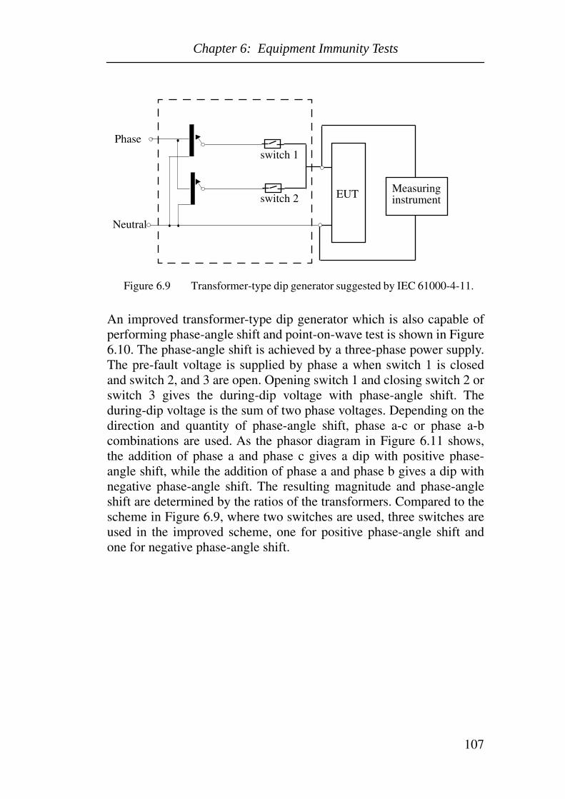
Chapter 6: Equipment Immunity Tests
107
An improved transformer-type dip generator which is also capable ofperforming phase-angle shift and point-on-wave test is shown in Figure6.10. The phase-angle shift is achieved by a three-phase power supply.The pre-fault voltage is supplied by phase a when switch 1 is closedand switch 2, and 3 are open. Opening switch 1 and closing switch 2 orswitch 3 gives the during-dip voltage with phase-angle shift. Theduring-dip voltage is the sum of two phase voltages. Depending on thedirection and quantity of phase-angle shift, phase a-c or phase a-bcombinations are used. As the phasor diagram in Figure 6.11 shows,the addition of phase a and phase c gives a dip with positive phase-angle shift, while the addition of phase a and phase b gives a dip withnegative phase-angle shift. The resulting magnitude and phase-angleshift are determined by the ratios of the transformers. Compared to thescheme in Figure 6.9, where two switches are used, three switches areused in the improved scheme, one for positive phase-angle shift andone for negative phase-angle shift.
Figure 6.9 Transformer-type dip generator suggested by IEC 61000-4-11.
EUT
Phase
Neutral
Measuringinstrument
switch 1
switch 2

Chapter 6: Equipment Immunity Tests
108
Figure 6.10 An improved transformer-type dip generator which is capableof performing magnitude, duration and phase-angle shift test.
Phase a
Phase b
Phase c
Neutral
EUT Measuringinstrument
Zer
o-cr
ossi
ng
dete
ctor
Inte
rfac
e
Con
trol
ler
switch 1
switch 2
switch 3
Figure 6.11 Phasor diagram of generating dips with phase-angle shift.
a
b
c
prefault voltage
Dip with positive phase-angle shift
Dip with negativephase-angle shift

Chapter 6: Equipment Immunity Tests
109
6.1.3 Test example
A dip generator set-up as shown in Figure 6.10 was used to performtests on a number of low voltage devices[59]. As an example, the testresults for a matrix printer are presented here. Figure 6.12 shows asimplified configuration of the power supply of the printer. The supplyconsisted of a transformer, a rectifier and a capacitor.
A single-phase dip with the following characteristics was applied to theprinter:
Magnitude: 70% Duration: 20 cyclesPoint-on-wave of initiation: 00
Point-on-wave of recovery:00
Phase-angle shift: 00
The results are shown in Figure 6.13.
Figure 6.12 Power supply of the printer
230 V ac
rectifier circuit
printer

Chapter 6: Equipment Immunity Tests
110
The ac current consists of two components: the magnetizing current ofthe transformer (the sinusoidal part of the pre-dip current) and the loadcurrent flowing through the transformer (spikes in the pre-dip current).During the dip the magnetizing current keeps on flowing, though lessthan normal. The load current ceases while the capacitor supplies theprinter. When the capacitor voltage has dropped below a certain level,load current starts to flow through the transformer again. When thevoltage recovers the capacitor is recharged to its normal voltage. Thiscauses the peaks in the load component of the ac current.
A voltage tolerance curve of the printer under test is produced. Theprinter is tripped below the curve. The dip is applied as the printer isprinting. A trip is defined as the stop of printing. The applied dipcharacteristics are as following:
Point-on-wave of initiation: 00
Point-on-wave of recovery:00
Phase-angle shift: 00
0 0.1 0.2 0.3 0.4 0.5 0.6 0.7-2.0
-1.0
0.0
1.0
0 0.1 0.2 0.3 0.4 0.5 0.6 0.7222630
3438
0 0.1 0.2 0.3 0.4 0.5 0.6 0.7-400
-200
0
200400
Vol
tage
(V
)V
olta
ge (
V)
Cur
rent
(A
)AC voltage
AC current
DC voltage
Time (second)
Figure 6.13 The test result of a printer during a 70% voltage dip.

Chapter 6: Equipment Immunity Tests
111
6.2 Three-phase equipment testThree-phase equipment is widely used in many different industries.Adjustable speed drives (ASD), and voltage source converters (VSC)are common three-phase equipment. Besides the dip characteristicsdescribed in Section 6.1 for single-phase equipment, for three-phaseequipment, the characteristics introduced in Chapter 3 should be used:characteristic voltage, PN-factor, zero-sequence voltage, next toduration, point-on-wave of initiation and recovery.
Currently used test methods simply combine three test setups forsingle-phase equipment to perform the test for three-phase equipment.However, as the previous chapters have shown, the three phasevoltages during a dip are following certain regularities rather thantaking random values, depending on the type of dip. Randomlychoosing test values has the risk of overestimating or underestimatingthe ride-through ability of the equipment under test (EUT).
The method of three-phase voltage dip classification proposed inChapter 3 facilitates the understanding of the dip characteristics duringits occurrence and propagation. Compared to the phase voltages, thecharacteristics, such as characteristic voltage, PN-factor, and zero-sequence, are much easier to set a range for equipment test. This range,
200 400 600 800 1000 12000
20
40
60
80
100
Time (ms)
Mag
nitu
de (
%)
Figure 6.14 Voltage tolerance curve of the printer

Chapter 6: Equipment Immunity Tests
112
which can be obtained either from theoretical study or from fieldmeasurement, provides a test environment closer to the reality.
6.2.1 Test items
A. Dip types
Chapter 3 classifies voltage dips experienced by three-phase equipmentas three fundamental types. Type A corresponds to the balanced dip.Type C and type D correspond to the unbalanced dips. If thesymmetrical phase is considered, type C and type D dips can be furtherclassified as six types: Ca, Cb, Cc, Da, Db, Dc.
The equipment should be tested for the three fundamental types. Thesymmetrical phase is not considered if the three phases of theequipment have equal status. In case additional power is taken fromone or two phases, like the field winding circuit of a dc ASD, theequipment should be further tested for the unbalanced dips withdifferent symmetrical phases.
The three-phase connection of the equipment under test (EUT) shouldbe indicated in the test result. For unbalanced dip test, a dip of type Dapplied to delta-connected equipment has the same effect as a dip oftype C applied to the same equipment with star-connection, and viceversa.
B. Characteristic voltage and duration
By classifying as different types, a three-phase voltage dip can bequantified by the characteristic voltage with an acceptable accuracylevel in most cases. The characteristic voltage is a complex number byits definition. The argument generally reflects the X/R ratio differencebetween the source and the faulted feeder. For a dip due to a fault in atransmission system, the argument is often around zero, thus thecharacteristic voltage is represented by a real number; for a dip due to afault in a distribution system, the argument is mostly negative.
The test should be performed first for zero argument of thecharacteristic voltage. In choosing the characteristic magnitude andduration, a table similar to Table 6.1 can be used. For unbalanced dips,a characteristic magnitude of 33% is suggested to be further tested. Thereason is that, for an unbalanced dip due to SLGF, where mostunbalanced dips are generated, the characteristic magnitude is notlikely to be smaller than 33%. This can be explained by (3.14). Since

Chapter 6: Equipment Immunity Tests
113
the zero-sequence source impedance (Zs0) generally has a bigger valuethan the positive source impedance (Zs1), the characteristic magnitudeis bigger than 1/3 of pre-fault voltage even for a SLGF at the PCC (Zf0=0, Zf1 =0).
Table 6.2:Preferred Characteristic voltage and Duration
The argument of the characteristic voltage, namely the characteristicphase-angle shift, can be added as a further test. The range of theargument depends on the system parameters, i.e. the X/R ratio of thesource and the feeders. Field measurements like shown in Figure 5.11and 5.12 can be used as a reference. The general trend is that a biggerargument is associated with a lower characteristic magnitude and thatonly negative argument values need to be considered. The preferredcharacteristic voltages and durations are shown in Table 6.2.
After setting down the test range of characteristic voltage, the phasevoltages of different types of dip are calculated from (6.1), (6.2), (6.3),which were derived in Chapter 3:
Type A:
(6.1)
Type C & Type D
Characteristic magnitude |V|
0 33% 40% 70%
Characteristic phase-angle shift arg(V)
-- -200 -150 -100
Type A Characteristic magnitude |V|
0 -- 40% 70%
Characteristic phase-angle shift arg(V)
-- -- -200 -150
Duration (in period) 0.5 1 5 10 25 50 X
Va V=
Vb12---V–
12--- jV 3–=
Vc12---V–
12--- jV 3+=

Chapter 6: Equipment Immunity Tests
114
Type C:
(6.2)
Type D:
(6.3)
Note: V, Va, Vb, and Vc are complex values.
C. PN-factor
Field measurements were shown in Chapter 5, resulting in, amongothers, values for the PN-factor of unbalanced dips. The conclusionfrom this was that the actual value of the PN-factor is close to unity.Only when large induction motor loads are connected to the system,the PN-factor deviates from unity. It is suggested to use a relationbetween PN-factor F and characteristic magnitude V as follows:
(6.4)
with f0 equal to 1, 0.95, and 0.9. The derivation of (6.4) can be found inAppendix B.
The phase voltages of type C and type D can be calculated by Equation(6.5) and (6.6) after the PN-factor is introduced.
Va 1=
Vb12---–
12--- jV 3–=
Vc12---–
12--- jV 3+=
Va V=
Vb12---V–
12--- j 3–=
Vc12---V–
12--- j 3+=
F f0 1 f0–( )V+=

Chapter 6: Equipment Immunity Tests
115
Type C:
(6.5)
Type D:
(6.6)
D. Zero-sequence
As mentioned before, the zero-sequence component rarely appears atthe equipment terminals. Only for SLGF and 2LGF zero-sequencevoltage occurs at the fault location. This component is blocked by mosttransformers; the exception is the star-star connected transformergrounded on both sides.
The zero-sequence component is normally only present in dips of typeD due to SLGFs. Theoretically, zero-sequence component could alsobe present in dips of type C due to 2LGF, but this is rather rare, andthus will be not considered in the test.
From the sequence network of SLGF shown in Figure 3.3, thefollowing relation between the zero-sequence voltage V0 and thecharacteristic voltage V is derived:
(6.7)
Va F=
Vb12---F–
12--- jV 3–=
Vc12---F–
12--- jV 3+=
Va V=
Vb12---V–
12--- jF 3–=
Vc12---V–
12--- jF 3+=
V0
Zs02
-------- 1 V–Zs1
-------------⋅=

Chapter 6: Equipment Immunity Tests
116
In a solidly-grounded system, the positive- and zero-sequence sourceimpedance can be assumed equal. The zero-sequence voltage can bechosen as
(6.8)
In case the source impedance at the point-of-common coupling isdominated by overhead line impedance, the zero-sequence groundimpedance may be twice the positive-sequence value. This leads to thefollowing relation:
(6.9)
In a high-impedance grounded system, a single-phase fault leads to acharacteristic voltage and a zero-sequence voltage both close to 1 pu.As the use of grounded equipment is extremely unlikely in high-impedance grounded systems, this case is not relevant for equipmenttest.
The zero-sequence voltage is opposite in direction to the characteristicvoltage. The presence of zero-sequence will even decrease the voltagein the symmetrical phase of type D, and swells may occur in the othertwo phases.
The phase voltages of type D dip can be calculated by Equation (6.10)after both PN-factor and zero-sequence voltage are introduced:
Type D:
(6.10)
E. Other test items
In case long post-fault dips are possible, it is recommended to test theequipment against it. The post-fault test can be performed as an
V012--- 1 V–( )=
V0 1 V–=
Va V V0+=
Vb12---V–
12--- jF 3– V0+=
Vc12---V–
12--- jF 3 V0+ +=

Chapter 6: Equipment Immunity Tests
117
additional type A dip immediately after the during-fault dip. The depthand duration should be obtained from a system study.
The point-on-wave of initiation is generally not considered in three-phase equipment tests, since the three phase voltages drop at differentpoints on the waveform. In case the point-on-wave is considered, thephase where the point-on-wave is specified should be indicated. Thepoint-on-waves of the other two phases have -1200 and +1200
difference.
The point-on-wave of recovery on three phases could be differentdepending on the coordination of the protection relay. The type of dipcould change during the dip recovery if the recovery instant is differentfor three phases. If the immunity of the equipment under test (EUT) isvery dip-type dependent, the test setup should simulate such aprocedure.
Source impedance: If the cause of equipment mal-operation is due toovercurrent or current unbalance, the source impedance is likely toaffect the immunity. Tripping on overcurrent may occur at voltagerecovery. Tripping on current unbalance may occur for three-phaseASD.
6.2.2 Test setup
The dip generator of three-phase equipment can again be put into twocategories: the amplifier-type and transformer-type.
The amplifier-type dip generator should be able to generate threeindependent waveforms to supply three phases of the equipment undertest. Three sets of the improved transformer-type dip generator shownin Figure 6.10 should be used, as phase-angle shifts always accompanyunbalanced dips. For both kinds of dip generator, the three phasesshould be coordinated to generate the intended type of dip.

Chapter 6: Equipment Immunity Tests
118
Chapter 7: Conclusions and Future Research
119
Chapter 7 Conclusions and Future Research
7.1 ConclusionsIn this thesis, a method for characterizing three-phase voltage dips isproposed and investigated. Under this characterization, three-phasevoltage dips are classified as three main types, denoted by A, C, and D.
Type A corresponds to balanced dips with an equal change in the threephases. Each balanced dip is quantified by its duration and acharacteristic voltage. The characteristic voltage is defined as thepositive-sequence voltage for balanced dips. The absolute value of thecharacteristic voltage (the characteristic magnitude) corresponds to thedip magnitude of each phase, while the argument of the characteristicvoltage (the characteristic phase-angle shift) corresponds to the phase-angle shift of each phase.
Type C and D correspond to unbalanced dips due to unbalanced faults.If the symmetrical phase is considered, unbalanced dips can be furtherclassified as six types, which are denoted by Ca, Cb, Cc, Da, Db, Dc.Each unbalanced dip is fully defined by its duration plus threecharacteristics:
•The characteristic voltage is the main quantifier for the severity of theevent. It is defined as the subtraction of positive- and negative-sequence voltage of type Ca, which is called a prototype dip. For manyapplications the characteristic magnitude (absolute value ofcharacteristic voltage) may be sufficient to characterize the event.
•The so-called PN-factor is a measure for the effect of the system loadon voltages at the equipment terminals during the fault. It is defined asthe summation of positive- and negative-sequence voltage of type Ca.Neglecting system load gives a PN-factor equal to one. In many casesthe PN-factor is close to one and can thus be neglected. The PN-factorneeds to be considered for specific applications in systems with a largeamount of induction motor loads.
•The zero-sequence voltage due to an earth fault rarely transfers downto the equipment terminals. Also equipment behaviour is rarelyaffected by the zero-sequence voltage. This characteristic is thereforeof minor importance.
Chapter 7: Conclusions and Future Research
120
A big advantage of the proposed classification method is thatcharacteristic magnitude plus dip duration are sufficient to characterizea three-phase voltage dip, either balanced or unbalanced.
The two-component symmetrical component method is used for thetheoretical analysis of dip classification. Positive- and negative-sequence source impedance are assumed to be equal in using thismethod. Various faults are analyzed by this method. The dip type andthe characteristics of voltage dips are defined based on the analysis.Mathematical models of transformers for voltage dip transformationare defined and studied. It is concluded that the transformers do notgenerate new types of dips but could change dip types. Mostimportantly, a type C and a type D dip change into each other through aDelta-Wye transformer. This reflects the internal relationship betweensingle-line-to-ground fault (SLGF) and line-to-line fault(LLF). Thephase-angle shift phenomena associated with voltage dips are alsoexamined. The phase-angle shifts in a balanced dip are caused by theX/R ratio difference between the source and the faulted feeder, whilephase-angle shifts in an unbalanced dip are the aggregation effect ofX/R ratio difference and three-phase unbalance.
The propagation of voltage dips requires different analysis tools indistribution systems and transmission systems. A voltage dividermodel can be used for studying both balanced and unbalanced dips in aradial distribution network. In transmission systems, however, thesituation is more complicated. Digital simulation has to be applied fora numerical solution. The proposed dip classification method greatlysimplifies the study of unbalanced dip propagation in power systems. Ifthe fault locations are the same, the characteristic voltage of dips fromthree-phase fault (3Ø), line-to-line fault(LLF), and two-line-to-groundfault (2LGF) are the same with the dip propagation; the characteristicvoltage of a dip from SLGF is the same as the characteristic voltage ofa 3Ø with an extra half zero-sequence impedance (Z0/2) connected atthe fault location; the PN-factor of the dip from 2LGF is the same asthe characteristic voltage of a 3Ø with an extra double zero-sequence(2Z0) at the fault place. Thus, a single-phase scheme is even capable ofstudying unbalanced dip propagation in power systems.
Dynamic loads, e.g. induction motor loads, have a strong influence ondip’s characteristics during their propagation. In a system where largeinduction motor loads are connected, a non-unity PN-factor of theunbalanced dip results due to two reasons:

Chapter 7: Conclusions and Future Research
121
•Positive- and negative-sequence impedances are different for thedynamic loads; The consequence of this is that, at any position in thesystem, positive- and negative-sequence impedance of the equivalentsource, are not exactly equal. This difference causes a non-unity PN-factor. The effect of induction motor load is a reduction of the PN-factor.
•The positive-sequence impedance of motor load decreases withincreasing motor slip. As motors slow down during a voltage dip, theload impedance will decrease with time during the dip. Because of this,the source voltage of the equivalent source will decrease with time,leading to a drop in the PN-factor.
Field measurements in both transmission systems and distributionsystems shows that the recorded dips can be classified as the proposedtypes. The PN-factors of the measured dips in transmission systems arevery close to unity; the PN-factors of the measured dips in distributionsystems are slightly less than unity. The characteristic voltage of bothbalanced and unbalanced dips show similar values. The characteristicphase-angle shift is close to zero in transmission systems, but mighthave a big negative value in distribution systems. The negative phase-angle shift in distribution systems is often larger for balanced dips thanunbalanced dips. The analysis of a propagating voltage dip from 132kV down to 33 kV and 11 kV shows increased characteristicmagnitude and decreased PN-factor from higher voltage level to lowervoltage level. The application of the classification method on a powerquality survey shows that this method has advantages in interpretingvoltage dip measurement. The waveform of the recordings can bereproduced with a reasonable level of accuracy. It is also shown that theshallow and unbalanced dips constitute the majority of the recordings.
Immunity testing of single-phase equipment against voltage dips is partof international standards. The dip magnitude and duration are themain concern for equipment immunity. However, other dipcharacteristics, e.g. phase-angle shift and point-on-wave could alsocontribute in tripping certain kinds of equipment. Thus, these non-energy-related characteristics should be also considered in the futurestandards. The dip classification method makes the immunity test ofthree-phase equipment against voltage dips more systematic. Sinceboth balanced and unbalanced dips can be mainly characterized by thecharacteristic voltage, the method developed for presenting single-phase immunity tests is easily adapted to three-phase tests by theseparation of different types of dip. In a more detailed test, the

Chapter 7: Conclusions and Future Research
122
additional characteristics, i.e. PN-factor, zero-sequence voltage, mightbe added.
7.2 Future ResearchDynamic loads have a strong influence on dip characteristics. Inductionmotor loads have been modelled and investigated. However, thesystem’s loads are complicated. Other dynamic loads, e.g. rectifierloads, could also affect the dip’s characteristics and the correctness ofthe classification method. The load’s effects on characteristic voltageand PN-factor needs to be further studied.
The phase-angle shift phenomena associated with both balanced andunbalanced dips are well explained by the fault analysis and themathematic dip model. However, the point-on-wave issue, which isrelated to the system fault characteristic and protection relay behavior,still lack information. The studies of the point-on-wave issue shouldcombine theoretical analysis with field measurements.
The dip classification method simplifies the dip propagation study forunbalanced dips, where a single-phase scheme is used. The conclusioncould be directly used by stochastic prediction of voltage dips, wherethe existing methods only concern balanced dips. The dip classificationmethod could adapt the existing method to unbalanced situations.
The dip classification method can have several applications for variouspower quality standards. The dip classification is quite promising inpresenting voltage dip measurements from power quality surveys. Thischaracterization can assist in further development of standards formonitoring voltage dips and for exchange of information betweenutilities, customers, and equipment manufacturers. Three-phaseequipment immunity tests against voltage dips is another application ofthe dip classification, in which it becomes critical to understand themagnitude and phase-angle shift relation of the unbalanced voltagedips. In development of equipment immunity test protocol, the testrange of characteristic voltage, PN-factor, zero-sequence, need to befurther studied with a consideration of statistics from fieldmeasurements.
Filed measurements have been obtained from various sources. Fieldmeasurements show that the classification method is valid for bothtransmission systems and distribution systems. Further statistics of dip

Chapter 7: Conclusions and Future Research
123
characteristics still need to be obtained from field measurements tocompare with the theoretical study. Several monitors should beinstalled at different voltage levels to measure the dip propagation.This can also help understand the change of dip type throughtransformers. The proposed classification method is based on severalassumptions. The limitation of the method should also be assessedthrough field measurements.

Chapter 7: Conclusions and Future Research
124

References
125
References
[1] R. C. Dugan, M.F. McGranaghan, H.W. Beaty, Electrical power systemsquality, New York: McGraw-hill,1996.
[2] M.F. McGranaghan, D.R. Mueller, and M.J. Samotyj, Voltage sags inindustry power systems, IEEE Transactions on Industry Applications,vol.29, no.2, pp. 397-403, Mar/Apr 1993.
[3] L.E. Conrad (Chairman), IEEE Std 493 Chapter 9, Voltage sag analysis,Power System Reliability Subcommittee Voltage Sag Working Group,draft 6 1995.
[4] M.H.J. Bollen, Understanding and Solving Power Quality Problems:Voltage Sags and Interruptions, New York, IEEE press, 1999.
[5] M.H.J. Bollen, Fast assessment methods for voltage sags in distributionsystems, IEEE Transactions on Industry Applications, vol.32, no.6,pp.1414-1423, Nov/Dec 1996.
[6] M.H.J. Bollen, Characterization of voltage sags experienced by three-phase adjustable-speed drives, IEEE Transactions on Power Delivery, vol.12, no.12, pp.1666-1671, October 1997.
[7] IEEE Project Group 1159.2, Task force on characterization of a powerquality event given an adequately sampled set of digital data points, firstdraft 1998.
[8] IEEE Std 1159-1995, IEEE recommended practice for monitoring electricpower quality, November 1995.
[9] CENELEC, Voltage characteristics of electricity supplier by publicdistribution systems, European Standard - EN50160, November 1994.
[10] Electromagnetic Compatibility (EMC), part 4. Testing and measurementprotocols. Section 11. Voltage Dips, short interruptions and voltagevariations immunity tests. IEC Document 61000-4-11.
[11] L.E. Conrad, M.H.J. Bollen, Voltage sag coordination for reliable plantoperation, IEEE Transactions on Industry Applications, vol.33, no.6,pp.1459 - 1464, Nov/Dec, 1997.
[12] P.M. Andersson, Analysis of faulted power systems, New York: IEEEPress, 1995.

References
126
[13] R. Collins, Waveform characteristics of voltage sags: definition andalgorithm development, Clemson University, South Carolina, March1998.
[14] L.D. Zhang, M.H.J. Bollen, A method for characterizing unbalancedvoltage dips (sags) with symmetrical components, IEEE PowerEngineering Letters, pp. 50-52, July 1998.
[15] L.D. Zhang, M.H.J. Bollen, Characteristics of voltage dips (sags) in powersystems, accepted by IEEE PES Transactions, in print.
[16] M.H.J Bollen, P. Wang, N. Jenkins, Analysis and consequences of thephase jump associated with a voltage sag, Power Systems ComputationConference, Dresden, Germany, August 1996.
[17] Measurement guide for voltage characteristics, UNIPEDE report 23003ren 9531. UNIPEDE documents can be obtained from UNIPEDE 28, rueJacques Ibert, 75858 paris Cedex 17, France.
[18] C.A. Warren, T.A. Short, J.J. Burke, H.Morosini, C.W. Burns, J. Storms,Power quality at champion paper - the myth and the reality, IEEETransactions on Power Delivery, vol.14, no.2, April 1999.
[19] A.V.Zyl, R.Spee, A.Favelike, S.Bhowmik, Voltage sag ride-through foradjustable-speed drives with active rectifiers, IEEE Transactions onIndustry Applications, vol.34, no.6, pp. 1270-1277, Nov/Dec, 1998.
[20] G.T. Heydt, W.T. Jewell, Pitfalls of electric power quality indices, IEEETransactions on Power Delivery, vol.13, no.2, pp. 570-578, April 1998.
[21] G. Yalcinkaya, M.H.J. Bollen, and P.A.Crossley, Characterization ofvoltage sags in industrial distribution systems, IEEE Transactions onIndustry Applications, vol.34, pp.682-688, 1998.
[22] IEEE P1346, Recommended practice for evaluating electric power systemcompatibility with electronic process equipment, 4th draft, September1996.
[23] IEEE guide for application of power electronics for power qualityimprovement on distribution systems rated 1kV through 38 kV, February1997.
[24] M.H.J. Bollen, The influence of motor reacceleration on voltage sags,IEEE Transactions on Industry Applications, vol.31, no.4, Jul/Aug 1995.

References
127
[25] G.Desquilbet, C. Foucher, P. Fauquembergue, Statistical analysis ofvoltage dips, 95NR00102, EDF, 1995.
[26] A.E. Turner, E.R. Collins, The performance of ac contactors duringvoltage sags, 7th International Conference on Harmonics and Quality ofPower, Las vegas, October 1996.
[27] A. Mansoor, E.R. Collins, R.L. Morgan, Effects of unsymmetrical voltagesags on adjustable speed drives, 7th International Conference onHarmonics and Quality of Power, Lars vegas, October 1996.
[28] M.H.J. Bollen, L.D. Zhang, Analysis of voltage tolerance of adjustable-speed drives for three phase balanced and unbalanced sags, IEEEIndustrial and Commercial Power Systems Technical Conference, Sparks,Nevada, May 1999.
[29] H. Seljeseth, A. Pleym, Spenningskvalitetsmålinger 1992 til 1996 ( voltagequality measurements, 1992 to 1996, in Norwegian), report EFI TR A4460published by EFI, 7034 Trondheim, Norway, March 1997.
[30] D.S. Dorr, M.B. Hughes, T.M. Gruzs, Interpreting recent power qualitysurveys to define the electrical environment, IEEE Transactions onIndustry Applications, vol.33, no.6. pp.1480-1487, Nov/Dec 1997.
[31] D.O. Koval, M.B. Hughes, Canadian national power quality survey:frequency of industrial and commercial voltage sags, IEEE Transactionson Industry Applications, vol. 33, no.3, pp.622-627, May/June 1997.
[32] D.O. Koval, R.A. Bocancea, K. Yao, M.B. Hughes, Canadian nationalpower quality survey: frequency and duration of voltage sags and surges atindustrial sites, IEEE Transactions on Industry Applications, vol.34, no.5,pp.904-910, Sep/Oct 1998.
[33] A. Burden, A. MacGregor, power quality initiatives at scottish power,Transmission & Distribution World, February 1998.
[34] SEMI F42-0699, Test method for voltage sag susceptibility ofsemiconductor processing equipment, SEMI online January 1999,http://dom.semi.org.
[35] P. Wang, The use of FACTS devices to mitigate voltage sags, PH.D thesis,UMIST, UK, July 1997.
[36] G.Yalcinkaya, The influence of induction motors on voltage sags due toshort circuits, PH.D thesis, UMIST, UK, October 1997.

References
128
[37] M.H.J. Bollen, P.Wang, N.Jenkins, Magnitude and phase-angle jump ofvoltage sags -- a theoretical analysis, submitted to IEEE Transactions onPower Delivery.
[38] M.H.J. Bollen, T. Tayjasajant, G.Yalcinkaya, Assessment of the number ofvoltage sags experienced by a large industrial customer, IEEE Transactionon Industry Applications, Nov/Dec 1997.
[39] M.H.J. Bollen, A.Mansoor, E.R. Collins, Characteristics of voltage sagsexperienced by single-phase and three-phase Equipment, PQA’97 Europe,Stockholm Sweden, June 1997.
[40] P.Rioual, J.L. Javerzac, F.de Chateauvieux, Characterization andrecognition of HV and EHV voltage dip signatures, PQA’97 Europe,Stockholm Sweden, June 1997.
[41] A.David, E. Lajoie-Mazenc, C.Sol, Ride-through capability of ACadjustable speed drives in regards to voltage dips on the distributionnetwork, EPE’93, the European Power Electronics Association, Brighton,1993.
[42] V.E. Wagner, A.A. Andreshak, J.P. Staniak, Power Quality and FactoryAutomation, IEEE Transactions on Industry Applications, vol.26, no.4, pp.620-626, Jul/Aug 1990.
[43] D.O. Koval, J.C. Chang, J. Leonard, Rural power quality, IEEETransactions on Industry Applications, vol.28, no.4, pp.761-765, Jul/Aug1992.
[44] M.R. Qader, M.H.J. Bollen, Stochastic voltage sag prediction technique,31st University Power Engineering Conference, Heraklion, Greece,pp.441-444, 1996.
[45] M. Morgan, M.Johans, Voltage sag mitigation through ride-throughcoordination, IEEE annual Textile, fiber, film conference, Greenville, SC,USA, pp.1-5, 1994.
[46] R.A. Epperly, F.L. Hoadley, R.W. Piefer, Considerations when applyingASD’s in continuous processes, IEEE Transactions on IndustryApplication, vol.33, no.2, pp. 389-396, Mar/Apr 1997.
[47] C.J. Melhorn, A.B. Braz, P. Hofmann, R.J. Mauro, An evaluation ofenergy storage techniques for improving ride-through capability forsensitive customers on underground networks, IEEE Transactions onIndustry Applications, vol.33, no.4, pp. 1083-1095, Jul/Aug 1997.
References
129
[48] C.J. Melhorn, T.D.Davis, G.E. Beam, Voltage sags: their impact on theutility and industrial customers, IEEE Transactions on IndustryApplications, vol. 34, no.3, pp. 549-558, May/Jun 1998.
[49] J.L. Zabala, S. Ruiz, G. Vargas, F. Soto, X. Prat, R. Barba,Characterisation of voltage dips in electrical networks and their Impact oncustomer installations, Cigre 21, rue d’Artois, F-75008 Paris.
[50] P.P. Khera, K.C. Dickey, Analysis and mitigation of voltage disturbancesat an industrial customer’s corporate campus, IEEE Transactions onIndustry Application, vol.34, no.5, pp. 893-896, Sep/Oct 1998.
[51] D.L. Brooks, R.C. Dugan, M.Waclawiak, A. Sundaram, Indices forassessing utility distribution system RMS variation performance, IEEETransactions on Power Delivery, vol.13, no.1, pp. 254-259, January 1998.
[52] A. Kara, P. Dahler, D. Amhof, H. Gruning, Power supply qualityimprovement with a dynamic voltage restorer (DVR), APEC’98, IEEEThirteenth Annual Applied Power Electronics Conference and Exposition,vol.2, pp.986-993 New York, 1998.
[53] K. Hadda, G. Joos, A fast algorithm for voltage unbalance compensationand regulation in faulted distribution systems, APEC’98, IEEE ThirteenthAnnual Applied Power Electronics Conference and Exposition, vol.2,pp.986-993, New York, 1998.
[54] Y.Kai, D. Koval, X. Wilsun, J. Salmon, An investigation of voltage sagsby phasor methodology, IEEE Canadian Conference on Electrical andComputer Engineering, vol.2, pp.689-692, New York, 1998.
[55] A.E. Turner, E.R. Collins, The performance of AC contactors duringvoltage sags, 7th International Conference on Harmonics and Quality ofPower, Las Vegas, October 1996.
[56] E.G. Strangas, V.E. Wagner, T.D. Unruh, Variable speed drives evaluationtest, IEEE Industry Applications Magazine, pp.53-57, Jan/Feb 1998.
[57] J. Holtz, W. Lotzkat, Controlled AC drives with ride-through capability atpower interruption, IEEE Transactions on Industry Applications, vol. 30,no.5, pp.1275-1283, Sep/Oct 1994.
[58] Manitoba HVDC Research Centre, PSCAD/EMTDC Manual, Winnipeg,Canada, 1992.
[59] J. Hilgers, Design and realization of a voltage sag generator, M.Sc thesis

References
130
No. 34 E, Department of Electric Power Engineering, Chalmers Universityof Technology, 1999.

Appendix A:Determination of Zero-sequence Source Impedance
131
Appendix A Determination of Zero-sequence Source Impedance
The power network’s zero-sequence source impedance is not alwaysknown. However, it can be determined from historical voltage diprecordings, together with the positive-sequence impedance of thesource and the feeders. Two cases will be considered below.
1. Both the positive-sequence source impedance at PCC and the feederpositive-sequence impedance are known. Only a dip from an SLGF atthe feeder is needed.
For a dip due to an SLGF at a distance, L from the PCC, thecharacteristic voltage VSLGF is:
(A.1)
where L is the distance from the fault to the PCC, Zs1 is the positivesource impedance at the PCC, Zf1 is the feeder’s positive-sequenceimpedance per kilometer, Z0 is the zero-sequence impedance at faultlocation.
Knowing the characteristic voltage VSLGF and the fault position L, wecan calculate Z0 from (A.1),
(A.2)
2. Only the feeder’s positive sequence impedance is known. A dip froma SLGF and a dip from a 3ØF , LLF or 2LGF are needed.
For a dip due to a 3ØF, LLF or 2LGF at a distance L from the PCC, thecharacteristic voltage V3Ø is
(A.3)
VSLGF
LZf1
Z02
------+
Zs1 LZf1
Z02
------+ +
-----------------------------------------=
Z0 2VSLGFZs11 VSLGF–----------------------- LZf1–
=
V3∅LZf1
Zs1 LZf1+---------------------------=

Appendix A:Determination of Zero-sequence Source Impedance
132
The positive-sequence source impedance can be calculated from (A.3),
(A.4)
and substituted into (A.2) to calculate Z0/2.
In transmission systems, the voltage divider model can not be used. Tocalculate the zero-sequence impedance Z0, the positive-sequencesource impedance at the fault point has to be known, and a dip fromSLGF has to be measured at the fault point. From (A.2) with L = 0, weget
(A.5)
Basically, zero-sequence impedance can be calculated by (A.5) in anysystems. But the problem is that positive-sequence source impedanceat the fault point and a measured dip at the fault point are also notavailable. More practical ways to obtain zero-sequence sourceimpedance in non-radial systems are still needed.
As an example, we use the dip data in Table 4.4 to calculate the zero-sequence source impedance. Faults at a feeder away from the 11 kVbus are chosen for calculations.
The first step is to calculate the positive-sequence source impedancefrom a 3ØF, LLF or 2LGF by (A.4). Given Zf1 = 0.1174+j0.3146ohm/km, L = 2 km, and V = 0.55∠-80, we get Zs1 = 0.03+j0.5628 Ω.
The second step is to calculate the half zero-sequence (Z0/2) from a dipcaused by SLGF by (A.3). Given Zf1 = 0.1174+j0.3146 Ω/km, L = 2km, and V = 0.69∠-50, we get Z0 = 0.2524 + j1.0532 Ω.
Zs1
1 V3∅–
V3∅--------------------LZf1=
Z0 2VSLGFZs11 VSLGF–-----------------------=

Appendix B:PN-factor and Characteristic Voltage
133
Appendix B: PN-factor and Characteristic Voltage
In a system where positive-sequence source impedance (Zs1) andnegative-sequence impedance (Zs2) are not equal, the PN-factor (F)will be not equal to unity. Besides, the PN-factor (F) also related thecharacteristic voltage (V). We will study the dips from SLGF and LLFseparately to give their relationships.
The standard voltage divider model as shown in Figure B.1 gets theform shown in Figure B.2 for SLGF and in Figure B.3 for LLF.
B.1 Single-line-to-ground Fault (SLGF)
Figure B.1 Voltage divider model
PCC
F
Load
Zs
Zf
+ -
VF
V2 V0V1
N1 N2 N0
Zs1 Zs2 Zs0
Zf1 + Zf2 + Zf0
Figure B.2 Sequence-network connection of SLGF
P1 P2 P0
+ - + - + -
Ia1 = Ia2 = Ia0

Appendix B:PN-factor and Characteristic Voltage
134
From Figure B.2, the three sequence voltages at the PCC are obtained:
(B.1)
According to the definition of characteristic voltage (V) and PN-factor(F) for SLGF in Chapter 3,
(B.2)
(B.3)
For Zs1 = Zs2 we obtain F = VF.
It follows from (B.2) and (B.3)
(B.4)
Note that this value is no longer dependent on the source voltage VF.All quantities in F/V are expected to be time-independent as well.
It also follows from (B.2)
(B.5)
V1 VF
Zs2 Zs0+( ) Zf1 Zf2 Zf0+ +( )+
Zs1 Zs2 Zs0+ +( ) Zf1 Zf2 Zf0+ +( )+----------------------------------------------------------------------------------------------=
V2 VF
Zs2Zs1 Zs2 Zs0+ +( ) Zf1 Zf2 Zf0+ +( )+
----------------------------------------------------------------------------------------------–=
V0 VF
Zs0Zs1 Zs2 Zs0+ +( ) Zf1 Zf2 Zf0+ +( )+
----------------------------------------------------------------------------------------------–=
V V1 V2+=
VF
Zs0 Zf1 Zf2 Zf0+ +( )+
Zs1 Zs2 Zs0+ +( ) Zf1 Zf2 Zf0+ +( )+----------------------------------------------------------------------------------------------=
F V1 V2–=
VF
Zs0 2Zs2+( ) Zf1 Zf2 Zf0+ +( )+
Zs1 Zs2 Zs0+ +( ) Zf1 Zf2 Zf0+ +( )+----------------------------------------------------------------------------------------------=
FV---- 1
2Zs2Zs0 Zf1 Zf2 Zf0+ +( )+-----------------------------------------------------------+=
Zf1 Zf2 Zf0+ +( )V Zs0 Zs1 Zs0+ +( ) VFZ
s0–
VF V–( )-----------------------------------------------------------------------=

Appendix B:PN-factor and Characteristic Voltage
135
Substitute (B.5) into (B.4),
(B.6)
where
(B.7)
B.2 Line-to-line fault (LLF)
From Figure B.3, the three sequence voltages at PCC are obtained:
(B.8)
F2Zs2
Zs1 Zs2+-----------------------VF 1
2Zs2Zs1 Zs2+-----------------------–
V+=
f0VF 1 f0–( )V+( )=
f0
2Zs2Zs1 Zs2+-----------------------=
-
+
P1
Ia0 = 0
N0
+
--
+Zs1
N1N2
Zs2
-
+Va1 Va2
Zf1 + Zf2
Ia1Ia2
VFZs1
P1 P2
Va0
Figure B.3 Sequence-network connection of LLF
Va1 VF
Zs2 Zf1 Zf2+( )+
Zs1 Zs2+( ) Zf1 Zf2+( )+---------------------------------------------------------------=
Va2 VF
Zs2Zs1 Zs2+( ) Zf1 Zf2+( )+
---------------------------------------------------------------=
Va0 0=

Appendix B:PN-factor and Characteristic Voltage
136
According to the definition of characteristic voltage (V) and PN-factor(F) for LLF in Chapter 3,
(B.9)
(B.10)
For Zs1 = Zs2 we obtain F = VF
It follows from (B.9) and (B.10)
(B.11)
It also follows from (B.9)
(B.12)
Substitute (B.12) into (B.11),
(B.13)
where
(B.14)
V V1 V2–=
VF
Zf1 Zf2+( )Zs1 Zs2+( ) Zf1 Zf2+( )+
---------------------------------------------------------------=
F V1 V2+=
VF
2Zs2 Zf1 Zf2+( )+
Zs1 Zs2+( ) Zf1 Zf2+( )+---------------------------------------------------------------=
FV---- 1
2Zs2Zf1 Zf2+-----------------------+=
Zf1 Zf2+( )V Zs1 Zs2+( )
VF V–( )---------------------------------=
F2Zs2
Zs1 Zs2+-----------------------VF 1
2Zs2Zs1 Zs2+-----------------------–
V+=
f0VF 1 f0–( )V+( )=
f0
2Zs2Zs1 Zs2+-----------------------=

Appendix B:PN-factor and Characteristic Voltage
137
The characteristic voltage and PN-factor follow the same relationshipfor both dips from SLGF and LLF. The constant f0, which isindependent of the fault reflects the system parameter’s influence onthe dip characteristics.

Appendix B:PN-factor and Characteristic Voltage
138