zePPeLIN: Ceiling camera networks for

the distributed path planning of ground

robots

A. Reina, L. Gambardella,M. Dorigo, and G. Di Caro

IRIDIA – Technical Report Series

Technical Report No.

TR/IRIDIA/2012-015

July 2012

IRIDIA – Technical Report SeriesISSN 1781-3794

Published by:IRIDIA, Institut de Recherches Interdisciplinaires

et de Developpements en Intelligence Artificielle

Universite Libre de BruxellesAv F. D. Roosevelt 50, CP 194/61050 Bruxelles, Belgium

Technical report number TR/IRIDIA/2012-015

The information provided is the sole responsibility of the authors and does not necessarilyreflect the opinion of the members of IRIDIA. The authors take full responsibility forany copyright breaches that may result from publication of this paper in the IRIDIA –Technical Report Series. IRIDIA is not responsible for any use that might be made ofdata appearing in this publication.

zePPeLIN: Ceiling camera networks for the

distributed path planning of ground robots

Andreagiovanni Reina1, Luca Gambardella2, Marco Dorigo1, Gianni A. Di Caro2

1 IRIDIA, CoDE, Universite Libre de Bruxelles - Brussels, Belgium

areina@iridia.ulb.ac.be, mdorigo@ulb.ac.be

2 Dalle Molle Institute for Artificial Intelligence (IDSIA) - Lugano, Switzerland∗{gianni,luca}@idsia.ch

Abstract

We introduce zePPeLIN, a distributed system designed to address the challenges of pathplanning in large, cluttered, and dynamic environments. The objective is to define the se-quence of instructions to move a ground object from an initial to a final configuration in theenvironment. zePPeLIN is based on a set of wirelessly networked devices, each equipped witha camera, deployed in environment. Cameras are placed at the ceiling. While each camera onlycovers a limited environment portion, the camera set fully covers the environment through theunion of the field of views. By local message exchanging, the cameras cooperatively computethe path for the object, which gets moving instructions from each camera when it enters cam-era’s field of view. Path planning is performed in a fully distributed way, based on potentialdiffusion over local Voronoi skeletons. The task is made challenging by intrinsic errors in theoverlapping in cameras’ field of views. We study the performance of the system vs. theseerrors, as well as its scalability for size and density of the camera network. We also propose afew heuristics to improve performance and computational and communication efficiency. Wereport about extensive simulation experiments and validation using real devices.

1 Introduction

In this work we present a distributed system for path planning. Path planning refers to the cal-culation of the path that an object has to follow for moving from a starting point to a givendestination/configuration. This is a fundamental problem in mobile robotics, where the movingobject can be the robot itself, a part of it (e.g., its robotic arms), or an object being carried byone or more robots. The calculation of a plan consists of the definition of the precise sequence ofroto-translations for moving the object without hitting obstacles or other robots. A large numberof different versions, algorithms, and solutions to this problem have been proposed in the last threedecades (e.g., see [13, 5, 14] for overviews). In this work we focus on the version which is also infor-mally referred to as the Piano mover’s problem. In this case, the controllable degrees of freedom ofthe moving object are equal to the total degrees of freedom, meaning that the moving object (thepiano) has not dynamic constraints on the motion (holonomic motion). The Piano mover’s prob-lem assumes that the agent who plans the path has as input the map of the environment and theobject’s model. However, in many practical cases, an input map including the precise deploymentof furniture and the status of other typical dynamic obstacles (e.g., a closed door, or the presence ofan occluding human crowd) is not immediately available. Therefore, in these cases, an up-to-datemap needs to be gathered on the spot prior to path planning. However, in the case of planning overlarge areas, this poses a clear problem, since in practice a collection of sub-maps, each referring to

∗This research was partially supported by the Swiss National Science Foundation through the National Centre ofCompetence in Research Robotics

1

a portion of the environment, needs to be gathered on the fly and possibly merged with each otherin order to perform a consistent and optimized path planning over the entire area.

To tackle this class of problems and, in particular, for planning the path of a holonomic objectof any shape over a large and cluttered area, we propose zePPeLIN (Path PLannIng Network),an approach based on the sensorization of the environment. A set of networked smart cameras isdeployed on the ceiling of the area where the object moves in order to visually cover the full area onthe ground. Camera deployment can be performed in any convenient way. In the following, withoutlosing generality, we assume the use of a swarm of flying robots, each equipped with a camera and awireless communication system (see the description of the robot camera model in the next section).Exploiting the top view, the camera system builds the map of the environment and the model ofthe moving object. Each camera of the network plans the local part of the path which is relative toits field of view. Then, it communicates with its neighbor cameras to locally merge the sub-pathsand to cooperatively generate a global path for the ground moving object. That is, the zePPeLINsystem plans the precise sequence of roto-translations that the moving object on the ground has toperform in order to reach its given final configuration. During path execution, each robot cameravisually localizes the moving object and sends to it the required motion information as it movesinto the wireless range of the robot camera itself. In this way, the use of the zePPeLIN networkedcamera system allows to effectively perform path calculations over large areas and can deal withdynamic changes in the environment by exploiting its parallel and distributed nature. Moreover,the system can be used to make path calculations for multiple ground-moving objects/robots atthe same time.

All these advantages have however a cost: the problem is made particularly challenging by thefact that each camera has a limited field of view, so that a camera can only see a limited portion ofthe environment, and the fields of views of neighbor cameras are partially overlapping, with inherentuncertainties in terms of mutual alignment and size of overlapping areas (a graphical illustrationof this is shown in Figure 2, explained in Section 4). The final global path is composed by partialpaths which are locally calculated and linked together in the overlapping areas. Wrong alignmentand overlapping information can lead the system to fail finding feasible paths. In fact, since eachcamera only calculates a partial path, if the information concerning the relative positioning ofthe overlapping area is erroneous, the linking of the local paths leads to imprecise, potentiallyunfeasible connections. During the phase of actual path navigation, some sub-path disconnectionscan be dealt by locally calculating repairing paths, which feasibly reconnect the sub-paths at theexpenses of some additional path length (see the discussion on navigation in Section 6). However,in a cluttered environment disconnected sub-paths may not have a feasible repairing path. In thiscase the calculated path is infeasible for navigation, resulting in a global failure. Therefore, animportant contribution of this work is the study of the robustness of the distributed path planningprocess to these errors, that are intrinsic to any distributed vision-based (or map-based) approach.Another contribution concerns the scalability of the system in terms of number of cameras and areasize in the presence of these same errors. To study these issues, we performed an extensive set ofexperiments both in simulation and using real cameras and moving robots. In order to improvethe efficiency and the accuracy of the distributed path planning process we also propose a set ofheuristics and we study their impact on performance. Moreover, we consider ways to reduce theimpact of camera alignment errors based on statistical reasoning.

In contrast to a centralized solution, where a single leading camera merges the visual informationfrom all cameras, the proposed zePPeLIN approach only relies on local and partial information.The entire process is fully distributed, and the communication between cameras is only local.Such architectural choices are motivated by the objective of obtaining a system which is scalable,robust to individual camera failures, and requires minimal communication overhead. In fact, with acentralized approach, the system suffers from the problem of the single point of failure and in orderto scale to large environments it has to cope with efficiency issues and communication bandwidthbottleneck. While these issues could be partially overcome with the use of effective ad-hoc routingalgorithms for communications, the zePPeLIN solution is still expected to be more general, portable,and efficient. It is also important to remark that an alternative approach based on the ground robotbuilding by itself the current obstacle map of the environment and performing self-localization (e.g.,a typical SLAM approach) and path planning, while potentially more precise, would require a much

2

longer computation and execution times than our approach (especially in the case of large areas),and would be more prone to path errors (e.g., while performing SLAM or moving through an area,the obstacle situation in nearby areas could have changed).

While in this introduction and in the rest of the paper we speak and makes use of vision-basedsensors to build local maps of the ground environment, we point out that the zePPeLIN distributedpath planning algorithm that we propose can be used with any system of networked devices capableof locally mapping the environment. For instance, a networked system of kinect-equipped or laser-equipped nodes could be equally used in the zePPeLIN framework, producing equivalent (if notbetter) performance of a camera-based system.

The rest of the article is organized as follow. In Section 2, we define the problem and thereference model used for the robotic ceiling cameras. In Section 3, we describe the state of theart methodology that we used to implement the distributed planner. In Section 4, we describethe distributed path planner. In Subsection 4.1, we propose a set of heuristics for improving theperformances of the system, that is, the quality of the solution and the efficiency of the process.Subsection 4.2 shows how the proposed system can deal with dynamic environments using localadaptation to changes of obstacle positions and camera failures. We present the results of thesimulation experiments in Section 5. The experiments are designed to study the performances ofthe system on the main aspects of interest: robustness, efficiency and scalability. Moreover, westudy how the various proposed heuristics affect the performances of the system. In Section 6, wedescribe the real robot experiments that we designed and implemented for validating the simulationresults. In Section 7, we list other works which address similar problems with a distributed or multi-agent approach. Finally, in Section 8 we conclude the paper with final remarks and the promisingdirection that will be investigated in future works.

2 Path planning scenario and camera network model

In zePPeLIN, we consider the following settings for the distributed path planning of a holonomicobject on the ground. At the beginning, a network of robotic ceiling cameras is deployed in theenvironment where the object moves. As pointed out in the previous section, at this aim we assumethe use of a swarm of flying robots each equipped with a camera. Each robot camera faces thefloor, in order to acquire a top view of the local environment underneath. The deployment is suchthat, altogether, the robot cameras cover with their visual field the ground environment includingthe start and the target position of the object. Robots are equipped with an on-board wirelesscommunication system. The deployment is performed such that the robots are locally in range witheach other and the fields of view of two neighbor robot cameras overlap. The size of the overlappingarea must be greater of or equal to the dimension of the moving object. This constraint is to allowthe cameras to connect sub-paths during the distributed path planning process by exchanging thelocal coordinates of the moving object. Once found their position in the environment, roboticcameras attach to the ceiling and keep a static position for the whole planning process. In this way,they can save energy while keeping monitoring the area. Since the focus of this work is on planning,we do not study how the camera formation can be obtained. However, in literature a number ofalgorithms that perform this kind of spacial deployment in the environment can be found, and anyof them could be used for this purpose (e.g., [26]).

We assume that the robotic cameras are equipped with a relative positioning system, whichallows a robot camera to estimate, with some uncertainty, the relative position (in terms of angleand distance) of neighbor cameras. This information is used to estimate the overlapping areabetween the fields of view of neighbor cameras and, in turn, to locally connect the sub-pathscalculated by each camera (see Section 4). Unfortunately, an error in the estimate of the relativeposition of two robot cameras results in an erroneous estimation of their overlapping fields of view,which can potentially have disastrous effects on the quality and feasibility of the calculated paths(see Figure 2). In this work, we study how the error in mutual positioning affects the performanceof the system, also in relationship to the number of robot cameras participating to the planningprocess. We consider this uncertainty as being an intrinsic issue of any vision-based distributedpath planning, and, as such, we consider it as an internal parameter of the problem. That is,

3

we do not propose ways to reduce it, for instance by means of sophisticated position calibrationtechniques; rather we empirically study to which extent this parameter impacts on the feasibilityand the quality of the planned paths. In the simulation experiments of Section 5 the error onrelative position and orientation is independently generated for each camera from two independentzero-mean Gaussian distributions with configurable standard deviation. In this way, we model errorestimates in a rather general and, at the same time, realistic way, avoiding to make assumptionsthat would be specific to the hardware in use.

As reference model for the robotic ceiling camera, we consider quad-rotor based flying robots.In particular, we consider the eye-bot [24], a quad-rotor flying robot equipped with a pan-and-tiltcamera that allows it to monitor what happens on the ground. The robots are also equipped witha Wi-Fi communication system and with a infrared range and bearing system (IrRB) [25], whichis used for calculating the relative position of other eye-bots and also provide a low-bandwidthline-of-sight data communication channel. We limit the set of neighbors of an eye-bot —i.e., thecommunication range— to the set of neighbors detected by the IrRB system (i.e., 5 meters). Aneye-bot can passively attach to the ceiling using a magnet, when a ferrous ceiling is present. In thiscase, the position of the robot camera is statically fixed and the robot can save energy, guaranteeinga relatively long operation time. Moreover, as typical quad-rotors can easily do, the eye-bot canalso hoover on the spot it has selected. In this way the system can be effectively used also inoutdoor environments (and in principle, to save energy, a robot can alternate between hoovering inthe air and resting on the ground when the moving object is not in its neighborhood). Clearly, inthis case the relative positioning error would fluctuate because of stability issues, introducing moreerrors that, however, could be smoothed out through repeated relative position exchanging usingthe IrRB system.

Since the focus of this work is on distributed path planning calculation, we make simplifyingassumptions for some of the aspects of the scenario that are not strictly related to plan calculations.In particular, we assume that the start and target configurations are given as input. Moreover,we assume that the moving object can be moved by a system that can interpret instructions givenby the zePPeLIN system (e.g., through a wireless system or a speaker). For instance, it can bea single ground robot, a set of assembled ground robots, or even humans (e.g., carrying a piano).In the real robot experiments of Section 6, the moving object that follows the camera instructionsis a two-robot system connected together in a rigid structure, and we consider an indoor scenariowhere the robots can keep static positions at the ceiling.

3 Path planning on a single environment map

The zePPeLIN system is based on the use of the partially overlapping vision maps of the envi-ronment gathered by the different robot cameras. Each robot camera performs path planningcalculations on its own local map, and it tries to optimally connect its path with that of the neigh-bor cameras through local message exchanges. Therefore, at first, each robot camera performs a“centralized” path planning calculation based on its local map, which includes also the overlap-ping areas with its neighbors. We designed and implemented this centralized planner by extendingcurrent state-of-the-art deterministic 2D path planning algorithms [13, 5, 14]. The developed cen-tralized planner is also used in the simulation experiments of Section 5 as baseline to assess theperformance of the zePPeLIN distributed approach. In this case, the planner takes as input, as asingle image, the entire view of the area where the object can move. The techniques, methods, andalgorithms that we used for implementing the centralized path planner are described in the rest ofthis section.

Environment model. The environment where the object moves, the ground, is modeled as aplane discretized in a uniform 2D grid of squared cells: the occupancy map. Each cell of theoccupancy map is labeled as free cell or occluded cell. The former are the cells that are free fromobstacles, meaning that the path of the moving object can pass through the area of the free cells.The set of the free cells is termed the free space. The occluded cells are the cells occupied, orpartially occupied, by an obstacle. Having a top view of the environment, the classification of the

4

cells in free or occupied is performed through a 2D isometric projection of the obstacles on theground. This way of proceeding might result in the definition of a subset of the actual free space,since the projection of some “table-like” object results in an occluded area, while in practice therecould be space for passing under it (depending on the 3D geometry of the moving object).

Potential field. The centralized path planning method we use is based on a classical work inthe field [13]. More specifically, we use the numerical potential field technique. First, a virtualpotential field is computed over the occupancy map, subsequently the path of the moving objectis calculated descending the gradient of the potential field. The potential field defines a force thatattracts the object towards the destination, and at the same time repels the object away fromobstacles. In our algorithm, the potential is a scalar function that defines the attraction/repulsionintensity for each cell. The function has a global minimum at the destination point, and maximumvalue on the obstacles. In all other cells the function decreases towards the destination, such thatthe planner can direct the object to the goal following the direction indicated by gradient descent.A 3D illustration of the potential field is provided in Figure 1a. The potential field is computedin three phases, described below: (i) calculation of the skeleton, (ii) diffusion of the potential fieldover the skeleton and (iii) diffusion over the remaining free cells.

Voronoi skeleton. The skeleton corresponds to the Voronoi diagram on the 2D occupancymap [28] (i.e., the set of points where the distance to the two closest objects is the same [5]).Since the planner operates on a discrete map, the skeleton is the subset of the free cellswhere the number of cells from the two closest occluded cells is the same. As final skeletoncalculation step, the destination cell is connected to the skeleton by a shortest line path (i.e.,the set of cells laying on the shortest line from the destination cell to the skeleton’s closestcell).

Diffusion over the skeleton. Once the skeleton is computed over the entire map, apotential field value is assigned to each cell of the skeleton. This operation is based on adiffusion process. The diffusion starts from the destination cell, to which a zero value ofpotential is assigned. A zero value means that there is no potential force when the objectlays on the destination cell. Then, the potential value is assigned to the neighbor cells ofthe set of the last cells to which a value has been assigned (after the first step, only thedestination cell belongs to this set). The new potential value assigned to the neighbor cellsis the potential value of the previous cells incremented by one. The process is iterated untilthe potential is diffused over all the cells of the skeleton.

Diffusion over the free space. After the skeleton cells have been assigned a potentialvalue, the potential field is computed over the remaining free cells. The diffusion process issimilar to the previous one. However, in this case the diffusion begins from the skeleton cells.In the case the importance of the skeleton needs to be enhanced —i.e., the desired path mustoverlap the skeleton— in the first diffusion step the increment of the potential value can begreater than one. In our algorithm we used 3 as incrementing value from the skeleton. Forthe subsequent diffusion steps, the incrementing value is fixed to 1. The process iteratesuntil the potential field is diffused over all the free space connected to the destination. Thevalue of the occluded cells is fixed to the maximum value. This means that a high repulsiveforce is applied to the cells occupied by obstacles (see Figure 1a for a graphical illustrationof the process).

Path calculation. The last phase of the planning algorithm consists in the actual calculation ofthe path. It is computed following the gradient in the descending direction. The process beginsfrom the starting position of the object and follows the decreasing value of the potential field.The potential field descent is computed using the least-cost finding A∗ algorithm [11]. In order toapply A∗, the 2D map is seen as a graph where the cells represent the nodes and there is an edgebetween two nodes when two cells are adjacent (i.e., we use Minkowski’s Taxicab Geometry [29]).

5

(a) (b)

Figure 1: Graphical representation of the potential field (a) and the moving object (b). Theenvironment is discretized in a 2D matrix of cells. The height and the saturation of the cellsrepresent the potential field value. Obstacles are represented by high brown cells, and the skeletonby the dark green graph. The moving object (the L-shaped green area) is represented by a set ofcontrol points (blue squares) and a set of collision points (purple squares).

The A∗ algorithm finds the least-cost path from the given initial cell to the destination cell. Ituses a distance-plus-cost heuristic function f(x) which is computed on every cell x visited by thealgorithm:

f(x) = g(x) + h(x) (1)

where g(x) is the path cost function and h(x) is the estimate function. The former represents thedistance from the starting cell to the current cell x. The latter is a heuristic estimate of the stepsfrom the cell x to the destination. This value is the value of the potential field.

Control points. We consider a moving object that can have any arbitrary shape and whose sizeis greater than the cell size. Therefore, it can occupy more than one cell. We use control points [5]to deal with this situation. The object is described by a set of control points, an example is shownin Figure 1b. At each instant the object is in a precise configuration, which corresponds to thespatial position and orientation of the object. A configuration c consist of the coordinates of thecontrol points, and the g(c) and h(c) values of Equation (1). The value of g(c) is the cost of all theunit movements from the start configuration to c. A unit movement can be either a translation ora rotation. The translation is of one cell in one of the cardinal directions (N, E, S, W, equivalentto up, right, down, left) and has cost equal to 0.5. A rotation of θ degrees can have place centeredon any of the control points, or on the center of mass of the control points, with θ a configurableparameter. The cost of a unit rotation is proportional to the number of traversed cells (in particular,it is the average number of cells traversed by all the control points). Therefore, an object with Ncontrol points has [4 + 2 ∗ (N + 1)] possible unit movements and neighbor configurations. The h(c)function is defined as the average over the potential value of all the control points. To describea configuration, an additional set of points is used, the collision points. These points lay on allthe cells occupied by the moving object’s perimeter (see Figure 1b). These points are not used forcalculating the function h(c), but are used instead for checking collisions with obstacles. In thecase a configuration has one (or more) collision points colliding with an obstacle, the configurationis not considered by the algorithm, being infeasible.

4 The distributed path planner

The centralized planner described in the previous section is the basic building block of the zePPeLINdistributed path planner: it is used by each individual camera for planning limited to its local

6

Figure 2: Illustration of how two neighbor camera nodes m and n define their overlapping regionand assign shared and open edges. δ is the relative position (in x, y coordinates) of the robotcamera node m in the reference system of n, α is the relative orientation of m with respect to theorientation of n. Using the δ and α estimates, node n builds a projection of the field of view ofnode m. In this way, node n defines the overlapping region (striped region), the shared edges (solidbold lines), and the open edges (dashed bold lines). δ and α are affected by the ε and ξ errorsrespectively. As discussed in Section 1, this results in an erroneous estimation of the overlappingarea, which can potentially have negative effects on the calculated path.

map. The distributed planner takes into consideration the whole set of local plans and defineways for their effective merging and coordination. The distributed algorithm is based on localsensing (the camera’s limited field of view), local communication between neighbor cameras, andpartial knowledge of the overall status of the planning process (no omniscient leader or centralizedcontroller exists).

The distributed algorithm presented in this section only executes path calculation, and it ter-minates when a valid path is found. The implementation of the path, that is, the actual navigationin the environment of the moving object is described in Section 6.

The zePPeLIN distributed path planning algorithm is composed of three phases, which aredescribed in detail below: (i) Neighbor mapping, (ii) Potential field diffusion, (iii)Path calculation.Figure 5 shows the zePPeLIN pseudo-code algorithm that is executed at a generic camera nodes;it includes both the local path planning and the navigation process.

Neighbor mapping. During this first phase, each camera estimates the overlapping area of itsfield of view with that of its neighbors. A robot camera n calculates the overlapping area betweenits field of view and the one of the its neighbor m in the following way (and repeats the sameprocess for all its neighbors). First, n collects two pieces of information: (i) the relative positionand orientation of m (measured using the range and bearing system); (ii) the size of m’s field ofview, received from m via wireless communication.

Then, with these two pieces of information it is able to calculate on its local 2D map theprojection of the field of view of m.1 Using the projection of the field of view of m, n calculates theoverlapping area, the open edges and the shared edges. The open edges are the edges of n’s field ofview that lay inside the m’s field of view. The closed edges are the edges of m’s field of view thatlay in n’s field of view. A graphical representation of this process is showed in Figure 2.

Potential field diffusion. Calculation of the potential field is the second phase of the distributedpath planning process. It is based on a diffusion process. Since each camera only sees a limitedpart of the environment, and the whole environment map is segmented across the networked camerasystem, robot cameras need to engage in a cooperative diffusion of the potential field. The processis fully distributed: starting from the cameras at the goal location, each camera first computesthe potential over its local map, then, it sends the potential field values of its shared edges to its

1As a simplifying assumption, we consider that all camera robots are placed at the same height, avoiding, in thisway, issues related to fields of view of different size.

7

neighbors, in order to allow them to continue with the potential field diffusion. From an operationalpoint of view, the process is implemented as follows.

Each camera calculates the local skeleton, which corresponds to the Voronoi diagram on its 2Doccupancy map (see Section 3). The environment’s skeleton resulting from the sum of all localskeletons differs from the one which would be calculated in a centralized way using a single globalmap. Differences are due to the fact that, during skeleton calculation, the frontiers of a (local)map need to be considered as obstacles. Therefore, at the corners of each map the local skeletonshows bifurcations that do not find their counterpart in the centralized skeleton (see Figure 3).Differences in skeleton turn into differences in the resulting path. This effect can be clearly observedfrom the results of the experiments with perfect alignment between cameras (see Section 5): thepaths planned with the distributed process and the paths planned by the centralized planner havedifferent length. An example of the paths generated by the global, single map planner and byzePPeLIN’s distributed planner is shown in Figure 4.

(a) (b)

Figure 3: Comparison of the skeletons.

Once the skeleton is generated, cameras cooperatively diffuse the potential, where the value ofthe potential field of each cell represents the number of steps from the destination to the currentcell. The cameras that have the goal configuration in their field of view start the process. Theyfirst diffuse the potential field on their local map. The diffusion starting point is the center of massof the control points of the goal configuration. Once the diffusion in the local map is completed,they send to the neighbors the value of the potential field on the shared edges. In this way, a robotcamera that receives this information can continue the diffusion starting from the values of thereceived edge cells. On reception, a camera copies the received values in the cells of its local map,and then executes the diffusion process on its local map starting from these received points. Eachcamera updates the potential value of a cell only if the new potential value is lower than the bestvalue it had calculated so far (i.e., a lower number of cells toward the destination is found). Thisprocess is iteratively executed in a distributed way among all the cameras in the network.

Cameras that have the final destination configuration in their field of view behave in a slightlydifferent way compared to the others. In fact, they need to precisely calculate the path that definesboth the final position and orientation of the object. For this, the use of the information regardingthe center of mass of the control points is not sufficient to guarantee the correct final orientation.Therefore, these camera calculate C different potential fields, one for each of the C control points.Each potential field is then diffused using as final destination point one of the control points. Duringpath calculation, these cameras compute the h(c) value averaging the potential field value of all thecontrol points. However, differently from the other cameras, for each control point the value whichis used is that of the corresponding potential field. In this way, during the third phase (see below),the cameras having the final destination in their view map can define the set of roto-translations ofthe object taking in consideration also its desired final orientation. Since only these cameras needto use multiple potential fields, this way of proceeding does not have a major impact in terms ofcomputation and communications, yet it is able to guarantee the correctness of the path.

In this same respect, it is important to remark that, in order to minimize communicationoverhead, with the aim of favoring scalability, portability, and of minimizing energy consumption,cameras communicate among them only the value of the skeleton cells laying on the shared edges.In this way, communication messages only contain the values of a few cells, resulting in a low

8

number of small packets of just a few bytes.

Figure 4: Final paths calculated by the global planner (Left) and by the zePPeLIN system (Right)in the same environment.

Path calculation. The third phase of the process consists in the actual calculation of the path,i.e., the definition of the sequence of roto-translations that connect the start and the final configura-tions. Each camera calculates the part of the path which is relative to its local map, and then sendsa message to one of its neighbors for letting it continue the planning. The process is implementedin the following way.

As in the previous phase, the camera that sees the moving object (that is, the start configura-tion), hereafter indicated with s, begins the third phase. Camera s calculates on its local map thepartial path of the object, ending on an open edge. Then, s randomly selects one of the neighborswith which it shares the open edge. Since each camera knows the projections of its neighbors’field of views (see Neighbor mapping of Phase 1), s can translate the coordinates of the movingobject from its frame of reference to the neighbor’s frame of reference. Finally, s sends these objectcoordinates to the neighbor, which then begins the local planning using as starting configurationthe object positioned at the received coordinates.

The process iterates among all cameras until one of the cameras calculates the partial path thatreaches the final configuration. When this happens, this camera broadcasts to all its neighbors asuccess message, which is flooded in a multi-hop fashion to all the other cameras in the network.In this case, the camera network has cooperatively found a path that connects the start and theend configuration positions. The information about the complete path is not stored in any specificcamera, but instead it is fully distributed in the network: each camera has the knowledge of onlythe partial path relative to its field of view. Once the path has been defined, the camera s triggerspath execution by communicating to the object the local information which is necessary to beginthe actual path navigation.

During the phase of path calculation, the camera can be in two possible states. In one state, itperforms the actual calculation of the partial path in its field of view, in the the other state it iswaiting for a message from neighbor cameras. There are 4 possible messages that a camera m canreceive from its neighbor n, which are listed below together with the actions that the reception ofone of these messages triggers:

• Start Path: This message contains the coordinates of the control points of the moving objectin m’s frame of reference. After receiving from a neighbor n a Start Path message, m startsthe path calculation using the received coordinates as start configuration. These coordinatesrepresent the final configuration of the partial path as calculated by n.

• Local Failure: This message is sent in response to a Start Path message when one of thefollowing two possible situations occurs: n has not found a valid path in its field of view,or the start configuration that has been included in the Start Path message is not-valid. Aconfiguration c is defined as not-valid when one or more of the following conditions hold: clays over an obstacle, c has already been evaluated by n during a previous path calculation, ccan be connected to a previous partial path calculated by n. The first operation that a camera

9

n does after receiving a Start Path message precisely consists in checking whether one of theseconditions is satisfied. In case the configuration c is not valid, then n replies to m with aLocal Failure message. After receiving this message, m sends a new Start Path message to adifferent neighbor laying on the same open edge on which the configuration c is positioned. Ifno alternative neighbors are present, camera m resumes the local path calculation from thestatus where it was before sending the configuration c.Through this process, when a camera does not find a local path, the system implementsa backtracking strategy: the control is given back to the previous node which searches foralternative solutions.

• Goal Found: This message notifies the successful completion of the path planning process.The camera that calculates the final part of the path (reaching the final configuration) locallybroadcasts to all its neighbors the Goal Found message, which is then flooded into the cameranetwork through multi-hop message relay.

• Global Failure: This message notifies a camera of a system-level failure for the path planningprocess. The system issues a global failure when all the configurations have been exploredbut the robot camera network is not able to find, in a distributed fashion, any path that canfeasibly connect the assigned start and end configurations. This means that a feasible solutiondoes not exist given the characteristics of the calculated potential field and the selected searchparameters (e.g., cell discretization, minimal rotation angle). A Global Failure message isgenerated first by the start camera, according to the following process. When a cameraexplores all the configurations in its field of view but has found no path that reaches thegoal or exits from an open edge, the camera asserts a local failure, as described above, andsends to the previous camera in the path a Local Failure message. Since its first selectionfor path continuation was aborted, also this camera can now possibly incur in an analogouslocal failure while trying to find an alternative path continuation. This potential sequence oflocal failures can let the system backtrack from camera to camera along the path built so far,until it reaches the first camera of the sequence, the one that started the planning phase andthat sees the start position. At this point no further backtracking is possible. Therefore, ifalso the start camera locally fails it means that the entire planning process has failed. In thiscase the Global Failure message is generated by the start camera and flooded in a multi-hopfashion throughout the camera network.

4.1 Heuristics

In the following two subsections we describe a set of heuristics that we designed to address the issueof getting trapped in local minima during the path search process, as well as issues related to thecomputational and communication efficiency of the system, with the aim of improving its overallscalability.

4.1.1 Heuristics to avoid local minima

During potential diffusion, the single-map path planner presented in Section 3 can potentiallyget trapped in local minima. This is due to the fact that potential diffusion does not explicitlyconsider the dimensions of the moving object, while path calculation does it. Therefore, when theshortest route towards the final configuration includes a narrow passage, the potential field candiffuse through the passage and assign low potential values to the corresponding area. During thepath calculation phase, the search algorithm explores the solution space expanding the search treetowards the areas with assigned low values for the potential field. In this way, the explorationprocess gets naturally attracted to the direction of the narrow passage and tries to establish apath through it. However, while the skeleton and the potential field were able to pass through thenarrow passage, the moving object has a shape and a dimension which might prevent its crossing.If this is the case, the process gets stuck exploring an area that has low potential values but whichis, at the same time, too narrow for letting the moving object pass through. In other terms, the

10

Algorithm 4.1 Local path planning and navigation algorithm executed at a camera node

1: M ← CalculateOccupancyMap() /* Detect obstacles and build local map */2: for all n ∈ Neighbors do3: CommunicateMyFoV Size(n)4: fovn ← GetNeighborFoV Size(n)5: δn ← DetectNeighborPosition(n)6: αn ← DetectNeighborOrientation(n)7: o← OverlappingArea(n, δn, αn, fovn)8: end for9: CalulateSkeleton(M)

10: if (isV isible(Destination)) then /* Camera with final configuration in the FoV */11: DiffusePotential(M,Destination) /* Potential field diffusion with Destination as starting point */12: SendPotentialF ieldMessageToNeighbors(M,N) /* Send the potential field on the shared edges */13: end if14: while potnew ← NewPotentialF ieldMessagesReceived() do /* Received updated potential field values

potnew from the neighbors */15: Diffuse potential(M,potnew) /* Potential field diffusion with potnew as starting points */16: SendPotentialF ieldMessageToNeighbors(M,N)17: end while18: while true do19: WaitForMessageFromNeighbors()20: i← ReadMessage(ni) /* ni is the sender of message i */21: switch (i)22: case StartMessage:23: si ← ReadMessageContent(i) /* si = starting configuration received with message i */24: if (isV alidStart(si)) then25: if (P ← CalculateLocalPath(si,M, o)) then /* The algorithm has found a local path P */26: if (P [lastPosition] = Destination) then27: LocalBroadcastGoalFound(N)28: go to: 5629: else30: sj , nj ← IdentifyNextNeighborInPath(P,N) /* sj = last position of the path P converted in

the reference system of neighbor nj */31: SendStartPathMessage(sj , nj)32: end if33: PATHS ← StoreLocalPathInfo(P, ni, nj , openset) /* openset = current status of the search */34: else35: if (isTheStartPositionV isible() AND isEmpty(PATHS)) then36: LocalBroadcastGlobalFailure(N)37: exit38: else39: SendLocalFailureMessage(ni)40: end if41: end if42: else43: SendLocalFailureMessage(ni)44: end if45: case LocalFailure:46: openset← RestoreP lanningStatus(PATHS[lastPosition])47: go to: 2548: case GoalFound:49: RelayMessage(i, N)50: go to: 5651: case GlobalFailure:52: RelayMessage(i, N)53: exit54: end switch55: end while56: k ← 157: if (isTheStartPositionV isible()) then58: go to: 6259: end if60: while NavigationCompleted do61: WaitForContinueNavigationMessage()62: NavigateTheRobot(PATHS[k])63: SendLocalNavigationCoontrolMessages(PATHS[k].next)64: k ← k + 165: end while

Figure 5: zePPeLIN pseudo-code: path planning process at a generic camera node.

11

(a)

(b) (c)

(d) (e)

Figure 6: Comparison of paths. (a) Global planner. (b) zePPeLIN planner without heuristics. (c)Planner using skeleton pruning (with the parameter wsp set to as the smallest dimension of theobject). (d) Planner using narrow passage detection. (e) Planner using all the heuristics.

search process gets trapped in a local minimum. The algorithm deals with this issue by locallybacktracking and exploring different alternative paths.

However, getting stuck in local minima and backtracking can have a significant negative impacton computational efficiency. Therefore, we propose two heuristics for minimizing the probabilitythat this happens: skeleton pruning and narrow passage detection. The two heuristics can beimplemented independently of each other and act in different phases of the process. The illustrationof the effect of the two heuristics, compared to the path resulting without the application of theheuristics, is shown in Figure 6.

12

Skeleton pruning. The aim of this heuristic is to prune the skeleton during potential fielddiffusion in order to block passages narrower than a predefined width wsp. In the experiments, weset wsp to the width of the smallest dimension of the moving object. However, since width is notthe only parameter defining whether an object can cross a passage or not (e.g., it depends alsoon the object’s morphology), the heuristic does not guarantee the removal of all local minima (seeFigure 7). On the other hand, setting wsp higher than the smallest object dimension, or, more ingeneral, too high, might result in the pruning of the majority of (or all) feasible paths.

Figure 7: Width is not the only parameter defining whether an object can cross a passage or not.In the two figures, the narrow passages of the two similar scenarios have the same width. Howeverthe object with L shape can pass through the passage of the right figure, while cannot for the oneof the left figure.

Narrow passage detection. This heuristic is executed during path calculation, when a cameradetects a local minimum due to the presence of a too narrow passage. A narrow passage is detectedwhen the following set of criteria is verified. Let x be the last visited configuration and b the visitedconfiguration with the lowest value of h(.). The heuristic checks the following conditions:

• [h(x) > (h(b) + 10)]: the search algorithm is exploring configurations with h value of oneorder of magnitude higher than the lowest visited. This means that the search algorithm isnot exploring configurations that reduce the distance from the destination.

• [∀cx /∈ skeleton] All the control points cx of the configuration x occupy cells that are notskeleton cells. Normally, the algorithm tends to calculate paths that follow the skeleton. Ifthe last visited configuration x is not on the skeleton, it is sign of anomaly (i.e., a possiblelocal minimum).

• [dist(x, b) > size(O)] dist(x, b) is the Euclidean distance between x and b, and size(O) isthe size of the largest dimension of the moving object O. This check aims to detect if thesearch algorithm has started to perform backtracking, or in other words, if the algorithm isexploring different alternative paths that are distant from configuration b, which the closestto the destination till now.

• [∃cbI /∈ freeSpace] Exists a control point cbI of the configuration bI that collides with obstacles(it is not in the freeSpace). Configuration bI is calculated starting from b and performinga 1-step translation in the direction of potential descent, i.e. in the direction to where thepotential decreases. This means that the algorithm stopped to visit configurations with lowerh value because an obstacle occludes the way.

When all the above criteria are verified, the camera has detected a narrow passage. At this point,the camera places a virtual obstacle over the cells belonging to the passage. The center centernp ofthe passage is identified as the cell of bI with lowest potential value. The algorithm places a virtualobstacle on centernp and on all the cells in the range of size(O)/2 cells from centernp. Then, ittriggers a new distributed potential field diffusion step that avoids in this way the passage, and,therefore, of being trapped in the associated local minimum.

13

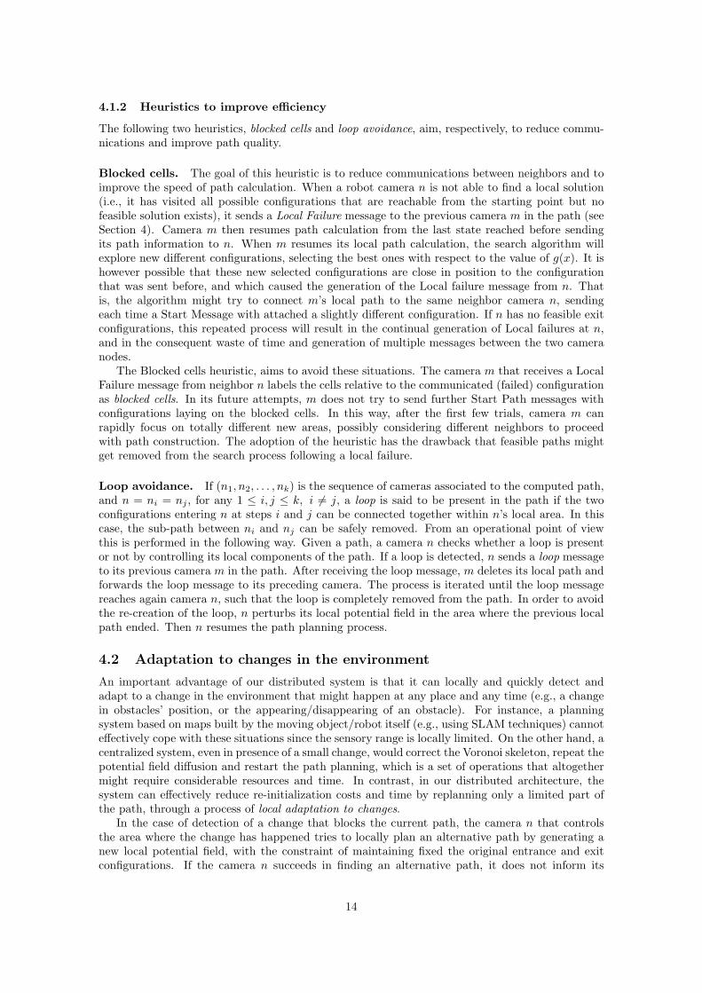
4.1.2 Heuristics to improve efficiency

The following two heuristics, blocked cells and loop avoidance, aim, respectively, to reduce commu-nications and improve path quality.

Blocked cells. The goal of this heuristic is to reduce communications between neighbors and toimprove the speed of path calculation. When a robot camera n is not able to find a local solution(i.e., it has visited all possible configurations that are reachable from the starting point but nofeasible solution exists), it sends a Local Failure message to the previous camera m in the path (seeSection 4). Camera m then resumes path calculation from the last state reached before sendingits path information to n. When m resumes its local path calculation, the search algorithm willexplore new different configurations, selecting the best ones with respect to the value of g(x). It ishowever possible that these new selected configurations are close in position to the configurationthat was sent before, and which caused the generation of the Local failure message from n. Thatis, the algorithm might try to connect m’s local path to the same neighbor camera n, sendingeach time a Start Message with attached a slightly different configuration. If n has no feasible exitconfigurations, this repeated process will result in the continual generation of Local failures at n,and in the consequent waste of time and generation of multiple messages between the two cameranodes.

The Blocked cells heuristic, aims to avoid these situations. The camera m that receives a LocalFailure message from neighbor n labels the cells relative to the communicated (failed) configurationas blocked cells. In its future attempts, m does not try to send further Start Path messages withconfigurations laying on the blocked cells. In this way, after the first few trials, camera m canrapidly focus on totally different new areas, possibly considering different neighbors to proceedwith path construction. The adoption of the heuristic has the drawback that feasible paths mightget removed from the search process following a local failure.

Loop avoidance. If (n1, n2, . . . , nk) is the sequence of cameras associated to the computed path,and n = ni = nj , for any 1 ≤ i, j ≤ k, i 6= j, a loop is said to be present in the path if the twoconfigurations entering n at steps i and j can be connected together within n’s local area. In thiscase, the sub-path between ni and nj can be safely removed. From an operational point of viewthis is performed in the following way. Given a path, a camera n checks whether a loop is presentor not by controlling its local components of the path. If a loop is detected, n sends a loop messageto its previous camera m in the path. After receiving the loop message, m deletes its local path andforwards the loop message to its preceding camera. The process is iterated until the loop messagereaches again camera n, such that the loop is completely removed from the path. In order to avoidthe re-creation of the loop, n perturbs its local potential field in the area where the previous localpath ended. Then n resumes the path planning process.

4.2 Adaptation to changes in the environment

An important advantage of our distributed system is that it can locally and quickly detect andadapt to a change in the environment that might happen at any place and any time (e.g., a changein obstacles’ position, or the appearing/disappearing of an obstacle). For instance, a planningsystem based on maps built by the moving object/robot itself (e.g., using SLAM techniques) cannoteffectively cope with these situations since the sensory range is locally limited. On the other hand, acentralized system, even in presence of a small change, would correct the Voronoi skeleton, repeat thepotential field diffusion and restart the path planning, which is a set of operations that altogethermight require considerable resources and time. In contrast, in our distributed architecture, thesystem can effectively reduce re-initialization costs and time by replanning only a limited part ofthe path, through a process of local adaptation to changes.

In the case of detection of a change that blocks the current path, the camera n that controlsthe area where the change has happened tries to locally plan an alternative path by generating anew local potential field, with the constraint of maintaining fixed the original entrance and exitconfigurations. If the camera n succeeds in finding an alternative path, it does not inform its

14

neighbors of the local change, and uses the new local path. Otherwise, n notifies the destinationnode (through multi-hop wireless communication) to trigger a new potential field diffusion process.The destination node decides either to repair the path (from n to the destination) or to recalculatethe entire path (using as start configuration the current position of the navigating object). Thedecision for either alternative is taken in relation to the position of n in the sequence of nodes alongthe path. E.g., a local repair is issued when n is close to the final destination. In this case, ifthe repair process happens while the object is already performing path navigation, it can continuethe navigation towards n, and when it will arrive at n a new path continuation toward the finaldestination will be already available.

4.2.1 Fault tolerance

Another possible change that can occur in the environment consists in the failure of one or morecameras (e.g., electrical failure, battery depletion). The zePPeLIN’s fully distributed architecturecan guarantee good levels of fault tolerance. In fact, in case a robot camera included in the pathfails and stops to work, neighbor cameras can rapidly detect the problem (cameras keep sendingeach other short keep-alive messages) and trigger a repair process similar to the one described inthe previous section. In this way, the network is able to find a new feasible path, if one exists,even in case of multiple camera failures. This capability is also observed in the experiments ofSubsection 5.3, where for large errors in relative camera positioning, systems with higher density ofcameras (i.e., greater number of cameras in the same environment) show a a better ability to findfeasible solutions compared to systems with lower densities. This is is due to the fact that whensome cameras fail in practice (due to the large error), other cameras can take their place in theprocess.

5 Results of simulation experiments

We studied the properties of the system through an extensive set of simulation experiments. Theexperiments have been designed with the objective of studying the following characteristics of thesystem: (i) the robustness to the alignment errors (i.e., wrong estimations of the neighbor’s relativeposition and orientation), (ii) the effect of the heuristics on performance, (iii) the scalability in largerenvironments (keeping the density of cameras constant), and (iv) the scalability for increasingdensity of cameras (keeping the environment size constant), which corresponds to scalability ofresources.

Performance metrics. The two main performance metrics we used for system evaluation arethe success ratio and the relative path length.

The success ratio is the percentage of successful runs over the total number of executed runs.The success of a run is determined with a post-evaluation of the resulting final path. As wedescribed in the previous sections, due to alignment errors the final path might be composed ofdisconnected sub-paths (Figure 2). The evaluation of the path consists in locally connecting thesub-paths to each other and in verifying its feasibility. This is done running the planning algorithmwith the starting and final configurations being respectively the last and the first configurations oftwo consecutive sub-paths. This evaluation permits to verify whether a solution has disconnectedsub-paths that can be feasibly reconnected during the navigation phase or not. If this is not the case,the disconnection results in an infeasible path, and therefore in a global failure. The reconnectionattempt is performed in a confined subregion, which is bounded by the field of view of the twocameras that have calculated the two sub-paths, and by a circular region with radius proportionalto the amount of the alignment error (higher error, higher radius). This spatial constriction aimsto find a local reconnection path which only includes a few roto-translations (i.e., a very shortsub-path), but not the definition of a completely new and alternative path which connects the twodisconnected sub-paths with a large sequence of movements and a long trajectory.According tothis validation procedure, a path calculated by zePPeLIN is classified as success, invalid, or failure.Success means that the system has found a solution and all the sub-paths can be feasibly connected.

15

Invalid means that the system has found a solution but the sub-paths cannot be connected. Failuremeans that the system has failed to find a potentially valid solution.

While the success rate in producing feasible paths is the first metric to assess the effectivenessof the zePPeLIN system, the length of the feasible paths also needs to be considered to assess itsperformance. Therefore, we considered as additional metric the ratio between the length of thecalculated path (including reconnection paths) and the length of the shortest path. The shortestpath is calculated on the global map by a centralized planner without any Voronoi skeleton. Thatis, the algorithm does not try to stay as far as possible from the obstacles. In this case, we do notcare of calculating a safe path which keeps a safe distance from the obstacles; rather the objectiveis to have the shortest possible path to be used as baseline reference. In the result plots showingrelative path lengths we indicate also the length of the path calculated by the centralized globalplanner with an algorithm identical to the one used in the distributed planner (i.e., using theVoronoi skeleton), but using a single global map.

General experimental setup. The experiments in simulation have been run with a dedicatedmulti-process simulator developed for this study. The input for one simulation experiment is aset of three files including: environment description, camera network formation, and parametricproperties. The environment description contains the set of obstacles on the ground with theirpositions and dimensions. The camera network formation file contains the list of all camera sensors,their positions, and their IP address. Parametric properties refer to the values of all the parametersthat characterize the system (e.g., the discretization step, the unitary rotation step, the activeheuristics, the standard deviation of the error in positional measurements, the communicationrange). A startup process reads the environment description and generates the image of the groundenvironment. Then, it reads the camera network file and launches an independent process for eachcamera passing as input: the portion of the ground image relative to the camera field of view, andthe set of neighbors (relative position and IP address). The set of neighbors is calculated in relationto the position of the camera and its range of communication. The environment description alsoincludes the start and final configurations of the moving object. All individual camera processescommunicate with each other and collaboratively plan the path.

The experiments have been run on a machine with 2 AMD Opteron 6128 (8 cores each, 2 GHz,2x 12 MB L2/L3 cache) and 16 GB RAM. The discretization of the environment for the purposeof defining unit movements amounts to 15 cells per meter, that is, cells with size of 6.7 cm. Asunitary rotation we used θ = 15◦. The moving object has an “L” shape with two segments ofsame length equal to 50 cm. In the planning process, the object is modeled by three control pointsas shown in Figure 1b. The simulation experiments are based on automatically generated maps,which differ in the placement of the obstacles. The maps are generated by placing every squaremeter a rectangular obstacle with probability 0.5. Obstacle placement is performed by randomlyselecting its position, orientation, and size (sampled between 20 cm and 1 m). The start and thefinal configurations are kept fixed for all the maps, respectively in the top-left corner and in thebottom-right corner.

In all the result plots, the performance of the system is evaluated against different levels oferror. Since the error is stochastically generated, we execute multiple runs for every error level inorder to improve the statistical significance of the results. For each error level we run 10 to 20 runs,depending on the experiment.

5.1 Robustness to relative position errors

In this section we present the results of simulation experiments designed to study the variation ofthe performance as a function of different levels of alignment error. We model the errors on relativeposition and orientation between cameras as two independent zero-mean Gaussian distributionswith configurable standard deviation. In the experiments, we vary the standard deviation of theerror on one measure, while keeping the error for the other measure fixed to zero. In Figures 8and 9, plots (a) and (b) shows the results for increasing angle errors, with the position error set tozero. The results for the reverse setup are shown in plots (c) and (d).

16

Experimental setup. For the experiments of Figures 8 and 9 we used 18 different maps of size12×7 m2 covered by a sensor network of 25 cameras, which have been deployed in the environmentin a grid formation of 5×5. Each camera has a field of view of 3×2 m2 of the ground, and thenetwork has a topology such that each camera’s field of view has a rectangular overlapping areawith the neighbor’s field of view of width equal to 75 cm.

0.70

0.80

0.90

1.00

Orientation error [degrees]

Suc

cess

rat

e

0 2 5 10

●

●

●

●

● No heuristicsWith Heuristics

(a)

0.70

0.80

0.90

1.00

Orientation error [degrees]

Suc

cess

rat

e0 2 5 10

●

●

●

●

● Blocked CellsLoop AvoidanceSkeleton PruningNarrow Passage Detection

(b)

0.70

0.80

0.90

1.00

Position error [m]

Suc

cess

rat

e

0.00 0.05 0.10 0.15 0.20

●

●●

●

●

● No heuristicsWith Heuristics

(c)

0.70

0.80

0.90

1.00

Position error [m]

Suc

cess

rat

e

0.00 0.05 0.10 0.15 0.20

●

●

●

● ●

● Blocked CellsLoop AvoidanceSkeleton PruningNarrow Passage Detection

(d)

Figure 8: Success rate of the system with respect to alignment errors: comparison of differentplanners. (a) Planners with and without heuristics varying the error in the relative orientation. (b)Planners with the 4 heuristics active independently varying the error in the relative orientation. (c)Planners with and without heuristics varying the error in the relative position. (d) Planners withthe 4 heuristics active independently varying the error in the relative position.

Results for robustness. Figure 8 shows that the success rate decreases with the increase of thealignment error. This is due to the fact that erroneous information of the overlapping area preventsthe connection of partial paths during the planning phase.

Figure 9 shows the results for the relative path length metric. Also in this case the performancesdecreases for high level of alignment error: the length of the final path is longer, thus less efficient(in terms of time and energy consumption). This is partially due to the connection paths, since thefinal path is the sum of the calculated sub-paths and the connection paths. When the error is high,the possible disconnection between paths is larger and consequently also the connection paths arelonger. This increases the length of the final path.

17

1.2

1.4

1.6

1.8

Orientation error [degrees]

Rel

ativ

e pa

th le

ngth

0 2 5 10

●

●

N H

●●●

●

N H●

● ●

N H

●

●

●

●

●

●

N H

G

●

●

●

N − No heuristicsH − With HeuristicsG − Global Planner

(a)

1.2

1.4

1.6

1.8

Orientation error [degrees]

Rel

ativ

e pa

th le

ngth

0 2 5 10

●

●

●

BLSN

●

●

●●

●

●

●

●

●

●

BLSN

●

●

●

●

●●

●

●

BLSN●

●

●

●●

● ●

BLSN

G

●

●

●

●

B − Blocked CellsL − Loop AvoidanceS − Skeleton PruningN − Narrow Passage Detection

(b)

1.2

1.4

1.6

1.8

Position error [m]

Rel

ativ

e pa

th le

ngth

0.00 0.05 0.10 0.15 0.20

●

●

N H

●

●●●

N H

●●

●

●N H

●

●●

N H ●N H

G

●

●

●

N − No heuristicsH − With HeuristicsG − Global Planner

(c)

1.2

1.4

1.6

1.8

Position error [m]

Rel

ativ

e pa

th le

ngth

0.00 0.05 0.10 0.15 0.20

●

●

●

BLSN

●

●

●

●

●

●

●

●

●BLSN●

●

●●

●

●

●●

●

BLSN●

●

●●

●

BLSN●

● ●●●

●

BLSN

G

●

●

●

●

B − Blocked CellsL − Loop AvoidanceS − Skeleton PruningN − Narrow Passage Detection

(d)

Figure 9: Relative path length for various levels of alignment error: comparison of different planners.(a) Planners with and without heuristics varying the error in the relative orientation. (b) Plannerswith the 4 heuristics active independently varying the error in the relative orientation. (c) Plannerswith and without heuristics varying the error in the relative position. (d) Planners with the 4heuristics active independently varying the error in the relative position.

Results for the impact of the heuristics. In Figures 8 and 9 we plot the results for thedifferent planners we propose. More specifically, we show the results of the planner with andwithout heuristics (on the left side) and the planners with each of the heuristic active independently(on the right side). The planner indicated in the figure as the ’planner with heuristics’ includedthree heuristics: blocked cells, narrow passage detection, and loop avoidance. We excluded skeletonpruning because of its low success ratio performance.

A first consideration is the positive effect of the heuristics on the quality of the solutions. Theplanner with heuristics is able to calculate on average shorter paths than the planner withoutheuristics (Figure 9a and 9c).

However, this beneficial effect has the disadvantage of a reduction of the success rate (Figure 8).With the increase of the error level, the success rate decreases more rapidly for the planner withheuristics than for that without heuristics. As described in Section 4.1, when the planner getsstuck in a local minimum, it executes a backtracking strategy which is resource demanding. Theplanning process in a local minima free scenario does not get stuck and rapidly finds a solution.The heuristics reduce the effect of local minima and improve the efficiency of the process (time

18

Pos. Err. Orient. Err. Normal BC LA SkP NPD All Heur.0 0 6.79 8.08 6.91 2.91 2.89 2.520 2 6.49 9.95 5.81 3.27 4.79 4.330 5 9.61 14.29 7.47 2.74 6.23 5.340 10 12.3 15.96 7.89 4.08 8.92 9.23

0.05 0 6.27 7.04 4.95 1.86 4.97 4.50.1 0 6.61 9.85 5.84 1.94 5.9 7.250.15 0 15.91 12.37 11.66 4.73 9.45 15.290.2 0 10.45 16.63 11.6 3.08 6.63 11.42

Table 1: Normal: without heuristics. BC: Blocked cells. LA : Loop avoidance. SkP: Skeletonpruning. NPD: Narrow passage detection. All Heuristics: BC + LA + NPD. This table shows theexecution time (in seconds) of the planners with and without heuristics with various levels of error.The value is the median of the distribution.

and messages) and of the solution (path length). However as drawback they reduce the solutionspace and feasible paths might get removed from the search process. The effect of each heuristic isdiscussed in separate paragraphs in the following.

The skeleton pruning heuristic aims to remove the local minima. It acts during the phase ofskeleton generation: it closes all the passages narrower than the object size. However, the object hasan L shape and it can thus overcome narrow passages with tight maneuvers between the obstacles.Therefore, in some environments this heuristic closes valid paths towards the destination. In thisway, it does not let the algorithm to find any valid solution. For this reason, the skeleton pruningheuristic noticeably reduces the success rate (Figure 8b and 8d). As an advantage, this heuristicslets the planner operate in a scenario free of local minima, so that the process can rapidly convergeto the solution without getting trapped. The effect is a more efficient planning process which avoidsbacktracking, and produces shorter paths (Figure 9b and 9d), has a quicker execution (Table 1),and generates a lower number of messages (Table 2).

The narrow passage detection heuristic is designed to remove local minima and their negativeeffects. It acts during the path calculation phase, and aims to block a passage only when theplanner has realized that it is effectively not feasible. This heuristic improves efficacy, in terms ofpath quality (Figure 9b and 9d) and efficiency, regarding execution time (Table 1), producing at thesame time less reduction of the success ratio compared to skeleton pruning, the other heuristic forlocal minima. A side effect of this heuristic is the higher number of messages it generates (Table 2).This is due to the fact that, when a camera detects a local minimum, it triggers a new potentialfield diffusion phase for the whole network.

The blocked cells heuristics aims to reduce the exchange of messages between neighbors. Table 2shows that the heuristic succeeds in this purpose. However, similarly to the other heuristics, it hasa lower success rate.

The loop avoidance heuristic aims to remove loops in the final resulting paths (see Section 4.1).That is, it aims to improve the quality of the resulting paths. Its effect is visible in the plots ofFigure 9b and 9d: the when the loop avoidance heuristics is active, the system can calculate thepaths with the shortest length.

5.2 Scalability to environment size

In this subsection we present the results of simulation experiments designed to study how the systemscales its performance when environment size increases. We consider environments whose size isrespectively two and three times larger than the size of a baseline environment.

Experimental setup. The experiments have been run considering 30 different maps with thefollowing sizes: 10 maps of 12×7 m2 (=84 m2), 10 maps of 12×14 m2 (=168 m2), and 10 maps12×21 m2 (=252 m2). Since environment size increases, also the camera network has to be increasedcorrespondingly to cover the entire area. In order to keep a minimum overlapping area of the fields

19

Position Error Orientation Error Normal BC LA SkP NPD All Heur.0 0 88.38 85.36 85.48 83.16 97.18 86.520 2 86.36 85 85.22 84.82 160.58 87.640 5 86.86 85.04 85.28 85.44 131.28 89.440 10 88.52 85.26 86.08 85.88 164.9 167.36

0.05 0 86.88 85.54 85.72 85.08 90.84 89.880.1 0 87.44 86.02 86.3 85.5 138.76 171.060.15 0 91.28 86 87.12 87.5 168.08 1710.2 0 89.92 86.16 87.08 86.8 145.68 174.54

Table 2: Number of messages per camera for the planners with and without heuristics with variouslevels of error. The reported value is the median of the distribution. Normal: without heuristics;BC: Blocked cells; LA : Loop avoidance; SkP: Skeleton pruning; NPD: Narrow passage detection;All Heuristics: BC + LA + NPD.

of view of 75 cm, the network scales to 5×11 cameras for the environments of double size, and to5×17 cameras for the triple size cases.

Results for efficacy and efficiency. Figure 10 shows the success ratio and the relative pathlength for different environment sizes. Both the effectiveness (success ratio) and the efficiency(relative path length) remain constant for larger environments. These results are indicator ofscalability for increasing environment size. Success rate values oscillate in a range between 100%and 93%. The plots in Figure 10a and 10b are jagged due to the strong heterogeneity of thescenarios and the random generation of errors. However, it is worth to notice, that the percentageof success remains over 93% also for high levels of error.

Boxplots in Figure 10c and 10d show the results in terms of relative path length. Also for thismetric the results confirm the scalability of the approach. While for environments of 84 m2 and252 m2 the relative path length values are very similar, for environment of 168 m2 the values areslightly higher (about 5%-10% more) and with higher variance. As discussed above, this differenceis due to the strong heterogeneity of the scenarios, which are randomly generated.

Figure 11 shows the efficiency of the system in terms of communication overhead. We study howthe number of messages varies scaling up the environment and the network. In order to performa fair comparison of the efficiency performance in the different environments, the reported valuesare normalized with respect to the average number of neighbors, which varies for the differenttopologies. In fact, the cameras on the edges of the network have a lower number of neighbors thanthe cameras in the middle. In our scenario, the cameras on the corner have 2 neighbors, the camerason the edge have 3, and the cameras in the middle have 4. To make the measure as independentas possible from this side effect, the reported values for the number of communicated messages arecalculated as follow:

Messages =1kN

N∑n

pn, (2)

where pn is the number of messages received by camera n, N is the total number of cameras, andk is the average number of neighbors in the network (for example in the case of a network 5×5,k = 3.2).

The number of messages increases with the network size. The cameras communicate the mostof the messages during the phase of potential field diffusion. This is due to the architecture of thesystem which waits for a fixed number of equal messages. When a camera receives from its neighborsthe same potential field message for more than 21 times, the potential is considered as definitive,and the camera terminates the diffusion phase. When the network size increases, the diffusionprocess takes more time, and as a consequence the number of messages (often repeated) increases.In our design, the bandwidth for messages was not an hard constraints, thus the message repetitionsolution has been implemented for simplicity. However, in case it is needed, communication duringthe diffusion phase can be optimized avoiding to communicate repeatedly the same message and

20

0.90

0.92

0.94

0.96

0.98

1.00

Orientation error [degrees]

Suc

cess

rat

e

0 2 5 10

●

●

●

●

● Normal200% Size300% Size

(a)

0.90

0.92

0.94

0.96

0.98

1.00

Position error [m]

Suc

cess

rat

e

0.00 0.05 0.10 0.15 0.20

●

●

●

●

●

● Normal200% Size300% Size

(b)

1.0

1.2

1.4

1.6

1.8

2.0

2.2

Orientation error [degrees]

Rel

ativ

e pa

th le

ngth

0 2 5 10

●

●

ND T

●

●●●

●

●●●●

●

●●

●

●●

●

●

ND T

●

●

●

●●●●

ND T

●

●

●

●

●●

ND T

●

●

●

N − NormalD − 200% SizeT − 300% Size

(c)

1.0

1.2

1.4

1.6

1.8

2.0

2.2

Position error [m]

Rel

ativ

e pa

th le

ngth

0.00 0.05 0.10 0.15 0.20

●

●

N D T

●●

●

●

●●●

N D T

●●

●

●●

●

●N D T

●

●

●

●

●

●

N D T

●

●●

●

●

●

N D T

●

●

●

N − NormalD − 200% SizeT − 300% Size

(d)

Figure 10: Scalability for environments with increasing size. (a) Success rate varying the error inthe relative orientation. (b) Success rate varying the error in the relative position. (c) Relativepath length varying the error in the relative orientation. (d) Relative path length varying the errorin the relative position.

designing the phase transition with another parameter (e.g., a temporal threshold from the lastreceived message). In fact, the number of messages communicated during the other phases is verylimited and remains constant for all the studied scenarios in a number ranging from 3 to 10 messagesper camera.

5.3 Scalability of resources

The set of experiments of this subsection shows how the performance of the system varies whenincreasing the number of cameras, while maintaining constant the size of the environment.

Experimental setup. The experiment setup is the same as in Subsection 5.1. We ran exper-iments over 10 maps, and for every map we increased the density of the camera network. Theinitial network is composed of a grid of 5×5 cameras, which is the minimum number to fully coverthe entire environment. We then increased the density by adding, in a first test case 25 cameras(+100% = double density), and in a second test case 50 cameras (+200% = triple density). In bothcases, the cameras were assigned with randomly selected position and orientation. For each of the

21

2030

4050

6070

80

Orientation error [degrees]

Mes

sage

s / c

amer

a

0 2 5 10

●

●

●

●

●

ND T

●

●

●

●

●

●●

●

●

●

●

●

●

●

●

●

●

●

●

●

●

●

●

●

●

●

●

●

●

●

●

●

●

●

●●

●

●

●

●●

●

●

ND T

●

●

●

●

●

●

●

●

●

●

●

●

●●

●

●

●

●

●

●

●●

●

●

●

●

●●

●

●

●

●

●

●

●●

●

●

●

●

●

●●

●

●

●

●

ND T

●

●

●

●

●

●

●

●

●

●

●

●

●

●

●

●

●●

●

●

●

●

●

●

●

●

●

●

●

●

●

●

●

●

ND T

●

●

●

N − NormalD − 200% SizeT − 300% Size

(a)

2030

4050

6070

80

Position error [m]

Mes

sage

s / c

amer

a

0.00 0.05 0.10 0.15 0.20

●

●

●

●

●

N D T

●

●

●

●

●

●

●●●

●

●

●

●

●

●

●●

●

●

●

●

●

●

●

●

●

●

●

●

●

●

●●

●●

●

●

●

●

●

N D T

●

●

●

●

●

●

●

●

●

●

●

●●

●

●

●

●

●

●

●

●

●

●

●

●

●

● ●●

●●

●

●

●

●

●

●

●

●

N D T

●●

●

●

●

●

●

●

●

●

●

●

●

●

●

●

●

●

●

●●

●

●

●

●

●

●

●

●

●

●●

●

●

●

●

●●●

●●●

N D T

●●

●

●

●

●

●

●

●

●

●

●

●

●●

●

●●

●

●

●

●

●

●

●

●

●

N D T

●

●

●

N − NormalD − 200% SizeT − 300% Size

(b)

Figure 11: Scalability for environment of larger size: efficiency measures. (a) Messages per cameravarying the error in the relative orientation. (b) Messages per camera varying the error in therelative position.

three setups we ran experiments varying the level of error on position and orientation and executing10 runs for each error level. This means that every point in the plots of Figure 12 corresponds tothe average of 10 · 10 = 100 runs.

Results. For high levels of error, the performance of zePPeLIN decreases: Figure 12 shows thesuccess rate as a function of alignment errors. These errors, in some cases, prevent connectionsbetween sub-paths in the overlapping area; therefore for high levels of errors the process more oftenfails to find a valid path. This negative effect can be reduced by increasing the number of cameras inthe sensor network (Figure 12). With the standard sensor network formation 5×5, the overlappingarea has a width of 75 cm and the moving object has a length of 50 cm. This formation has alimited margin of error, which allows the system to cope effectively only with low levels of error(success rate over 95% (first dot of plots in Figure 12). A more dense network has wider overlappingareas, which is aspect that allows the system to effectively plan valid paths more often and evenfor high levels of errors.

The system improves its performances in response to an increase of the resources in the system(i.e., the number of cameras in the sensor network). In zePPeLIN, the increase of resources is easedby a distributed, scalable and flexible architecture, which is designed to allow the user to add newcameras without any need to modify, update or setup the algorithm.

6 Real robot experiments

We completed the experimental evaluation of zePPeLIN with a set of experiments with real camerasand ground robots. In these experiments, zePPeLIN executes all planning and navigation phases:it detects moving robot position, it calculates the path from the current position to the givendestination, and provides the instruction to navigate the ground robots in the environment. Thesetup adopted for the real world experiments and the results are described in the rest of the section.

The environment. The ground robot moves in an area of 33 m2 where the gray floor is occludedby red obstacles. This color configuration has been selected for easing the obstacle detection sinceit is not the main focus of the work. A sample image of the arena is shown in Figure 13 (Left).

22

0.70

0.80

0.90

1.00

Orientation error [degrees]

Suc

cess

rat

e

0 10 20 30

●

●

●

●

● 25 cameras50 cameras75 cameras

(a)

0.70

0.80

0.90

1.00

Position error [m]

Suc

cess

rat

e

0.0 0.2 0.3 0.4

●

●

●

●

● 25 cameras50 cameras75 cameras

(b)

Figure 12: Scalability for higher number of cameras keeping the environment size constant. (a)Success rate varying the error in relative orientation. (a) Success rate varying the error in relativeposition.

Figure 13: Scenario for real robot experiments. (Left) An example arena. The moving object hasto move in the arena avoiding collision with the red obstacles. (Right) The moving object thatfollows camera instructions, which is implemented as a set of 2 e-puck robots interconnected by arigid structure.

The camera network. The robotic camera network is implemented with a set of 4 cameras,fixed at the ceiling, pointing to the ground and connected to different computers. Each camera iscontrolled by an independent process, which cooperates and communicates wireless with the otherprocesses via UPD sockets. The cameras are placed at an height of 3 m and have a field of view of4.56×3.06 meters with an image resolution of 640×480. In our experimental setup we used normalcameras, that cannot autonomously estimate their relative position with respect to the neighborcameras. For overcoming this issue, for each camera an input configuration file specifies the IPaddresses and the relative positions of its neighbors. The cameras are deployed in a rectangularformation, such as each camera has an overlapping field of view with two neighbor cameras. Allthe cameras have the same orientation, relative distances of 3 m (with the neighbor on the x axis)and 2.38 m (with the neighbor on the y axis), and a communication range limited to 3.5 m. Theerror on the measures of the relative distances and orientation is of the order of 0.1 m and 10◦

respectively.

The moving robot. The holonomic object moving on the ground is implemented as a set of twonon-holonomic robots, the e-puck [17], interconnected by a rigid structure (see Figure 13, right).Each robot can freely rotate on place, while straight direction movements are constrained by the

23

rigid structure and must be executed in coordination between the two robot. In this way, thetwo robots form an object with a relatively large shape, which is able to rotate and move in anydirection. As discussed in Section 3, the path planning algorithm models a moving object by usingcontrol points. In this case, the control points corresponds to the center of the two e-pucks. Eachof the two e-pucks has a colored patch applied on its top, in order to allow the cameras to tracktheir positions and orientations.

The path planning process. Each camera is controlled by an independent process. Trougha graphical interface, the user connects to a desired camera and specifies the final position andorientation of the object. The camera system autonomously detects the obstacles and the currentposition of the moving robot in the environment. With this information, the system calculates thepath from the start to the final configuration in a distributed way, where each camera operates onlyon its local field of view. The resulting path is the ordered sequence of local configurations (i.e., anordered sequence of roto-translations), where each camera holds the sequence relative to its field ofview.

The navigation in the environment. Once the path is defined, the system starts the navigationphase. The navigation control process cs connected to the camera s that has the moving robot in itsfield of view starts the navigation phase. Using the camera, process cs tracks the current positionof the two e-pucks and sends them via Bluetooth two independent messages with the informationof the relative movement to be performed, that can be either a rotation in place or a translation.Each e-puck, when it completes the required movement, sends a notification message back to cs.Iteratively, using the current position of the two robots and the next configuration to be reached, asspecified by the locally planned path, the control process calculates and sends the relative movementthat each robot has to perform next. In this way the camera-robot system operates in a closedloop, such that it is able to correct possible path implementation errors.

When process cs navigates the robots to the last position of the its local path ps, it communicateswith the navigation control process cn of the next camera n in the path in order to let it take controland continue robot navigation. It might happen that the e-puck system completely enters the fieldof view of n before the execution of path ps is completed (e.g., because of little errors in navigation,or because of a relatively large overlapping between the fields of view). When this happens, sinceprocess cn has better information than cs regarding its local environment, it is appropriate that ntakes control. Therefore, n tries to plan a local path pconn which connects the current position ofthe robots to the closest point of the calculated path pn. If a connection is found, it means thatn can locally navigate the robots to a configuration in pn and continue the navigation on pn asexpected. In this case, the process n sends a messages to process cs requesting the control. On thereception of this message, cs interrupts the navigation and hands the control to cn.

The process described for cameras s and n is then iterated between all cameras involved in theplanned path, until the moving robots reach the desired destination. A few sample videos showingpath calculation and path navigation are available at the supplementary page2. The videos areshown three times faster than reality. In the videos, when a camera passes the navigation controlto the next camera, a connection path is calculated, which is drawn in yellow. A camera icon showswhich camera is taking control. Every time the control is passed from one camera to the next onethe two robots rotate in place before starting to move. This is due to the following reason. Inorder to make the tracking process simple and scalable, the same color patch is put on the top ofthe two e-pucks, such that there is no need to create new custom patches if new robots are addedto the multi-robot structure. However, this way of proceeding has the drawback that the trackingsystem has no way to to distinguish between the two e-pucks, which is needed because each e-puckhas to perform different movements and the control process has to send different messages to eachof them. Therefore, before starting to send instructions, the control process sends, in sequence, amessage to each one of the known addresses of the two e-pucks, asking to perform a rotation inplace. This allows the control process to associate each robot to its wireless address.

2The videos are available at http://iridia.ulb.ac.be/supp/IridiaSupp2012-013/index.html

24

Experimental results. We performed experiments on 20 different maps: in 14 of them theenvironment is relatively well structured, with the obstacles placed to form straight walls (seeFigure 14a for an example), while in the remaining 6 the obstacles are deployed completely randomly(see Figure 14b for a sample scenario). In all the experiments, the system has been able to calculatevalid paths no longer than 150% of the optimal shortest path, and 115% of the path calculated bythe global planner. Figures 14a and 14b show the composite screen-shot of the 4 fields of view.Planning time is relatively low, for example the planning time for the paths shown in Figures 14aand 14b is respectively of 4.6 s 7.2 s.

From the mentioned sample videos, it is possible to appreciate that the robots implementingthe instructions received from the overhead camera are able to follow the calculated path with goodprecision. The system is able to effectively correct local actuation errors through the continuoustracking of the positions and recalculation of the next relative movements to communicate.

(a) Structured environment. (b) Randomly displaced obstacles.

Figure 14: Composite screen-shot of the four fields of view of the four cameras in two differentexperimental setups. The planned path (in red the control points and in white the stylized object)is shown. In this example, the information of the final path is segmented in three partial pathsdistributed among the cameras.

7 Related work

Path planning is a fundamental problem in mobile robotics and for this reason it has been extensivelystudied, mainly considering centralized and single-robot approaches. An overview of the establishedwork in this respect can be found in [13, 5, 14]. However, recently, there is increasing interest fordistributed approaches in robotics, and this applies also to path planning. Work on distributedpath planning can be roughly grouped in four main research threads: (i) on-board multi-robotpath planning, (ii) path planning assisted by a sensor network, (iii) swarm approaches, and (iv)parallelism of computation. Our work belongs to the second thread. in the following we brieflydiscuss some of the most prominent approaches for all the considered threads of research, with aparticular emphasis on the second one.

On-board multi-robot path planning studies [9, 2, 18, 21] propose distributed planning andnavigation algorithms for letting a group of robots moving in the environment without collidingwith the obstacles and with each other. Each work is usually based on different assumptions andproblem statements, which also makes relatively difficult to draw proper comparisons among thedifferent approaches. In [9, 18] the authors investigate how the multi-robot system behaves varyingthe noise in sensor measurements. In [23] the goal is to keep a predefined formation of the group ofrobots while moving towards a given destination. In all these works the algorithm runs on-boardof the robot, thus the path is planned directly by the robot which then implements it. Robotsneed to know the map of the environment. This information can be either given as input or the

25

robots can locally sense and explore the environment and generate a map on the fly (e.g., using aSLAM technique). Both approaches are however not able to deal robustly with large and dynamicenvironments, which, on the other hand, are the class of environments we target with our system.

Path planning assisted by a sensor network has been considered in a number of worksin the last decade [16, 1, 15, 6, 3, 20, 30, 7]. In the considered scenarios, the moving robot is notrequired to be equipped with sophisticated devices and powerful CPUs in order to perceive theenvironment, build a representation of it (i.e., a map), and calculate a motion plan. Instead, therobot is guided by a distributed sensor network deployed in the environment. Compared to thesingle robot, the sensor network can exploit a better and distributed point of view, can rely on amuch wider coverage of the environment, and can quickly react to changes in the environment orin the network (even if these happens at locations distant from the current position of the movingrobot). In these works based on the use of an external sensor networks, the resulting path iscommonly defined as the sequence of sensors that the moving robot has to visit. Sensors act asrouters and compute only the high level plan (i.e., the direction towards the next sensor). Whenentering the communication range of a sensor, a robot gets the necessary instruction to proceedwith the plan. The robot is in charge of planning and implement the precise sequence of roto-translations for moving toward the next router while maneuvering between the obstacles and othermoving robots. The planned path consists of a sequence of nodes. Obstacles in the environment areusually not explicitly considered, assuming that there is always a valid path between two neighborsensors and the moving robot is able to effectively sense the environment and compute local motionplanning. The path planning problem is therefore reduced to compute the shortest path on a graph,where the sensors are the nodes of the graph and some notion of neighborhood (e.g., wireless range)defines that two nodes are connected by an arc that can be navigated by the robots. In this samecontext, some works have studied the path planning problem considering additional constraintssuch as: avoidance of dangerous areas [15, 3], collision-free trajectories for multi-robot systems [16],presence of different terrain surfaces (which results in different motion speeds) [30]. The algorithmpresented in [31] makes use of a sensor network with complex spatial sensing capabilities. Theauthors of the paper propose the Distributed Probabilistic Roadmaps algorithm where each sensorcalculates a part of the path in the area in its sensing range and joins its sub-path with the oneof its neighbors in a shared area of overlapping sensing. The resulting path is the sequence of thevia-points that allow to avoid collisions with obstacles and to safely reach the next sensor/router.This study presents strong similarities with our work: the generated path is sufficiently detailedand takes in account the size and the shape of the moving robot. However, the authors do notreport any study on the impact of measurement errors for the overlapping areas, which is one of thefocus of our work being this a sort of intrinsic aspect of distributed sensory and planning systems.

Swarm robotics systems are characterized by large number of robots and the use of localcommunications and self-organized cooperation. Works in literature exploit these aspects to performswarm-level path planning. In [22] the system assumes that a dedicated sensor network is deployedin the environment which navigates the swarm, similarly as it happens in the case of the worksmentioned above based on the use of external sensor networks. In [19] the algorithm exploits thesame robots in the swarm for creating a chain of static landmarks to navigate the other robots in theenvironment. In [10, 4, 8] the system does not allocate (and fix) any specific resource for building adedicated sensor network, but the swarm itself is a mobile sensor network. Each robot while movingin the environment acts as landmark communicating information for the localization of the localneighbors and at the same time receives information from the neighbors. In all these works, both thesensors and/or the robots do not calculate the precise path through a cluttered environment, butact as high level routers which direct the moving robots to the next sensor/robot communicatingonly the direction. The final path consists of the sequence of sensors to be visited, which is verydifferent from our work where the resulting path is the precise sequence of roto-translations to beperformed to move through a potentially highly cluttered environment.

Parallelism of computation consists in distributing the planning computation on differentprocessors for increasing the overall computational speed of the system [12, 27]. In these works,differently from ours, the computing nodes have a global knowledge of the environment, and theissue is how to optimize the division of computation. A different approach to parallelism is takenin [21], where the authors cast a multi-robot system as a distributed multi-computer, with each

26

robot calculating a (possibly different) solution based on a rapidly-exploring random tree techniquewhich is shared with the other robots according to communication conditions. Using this approach,the algorithm is meant to exploit perfect communication and have gracefully performance declineotherwise.

8 Conclusions and future work

We have proposed zePPeLIN, a novel system for distributed path planning in large, cluttered, anddynamic areas. The system is based on a fully distributed architecture, in which a swarm of fly-ing robots is deployed in the environment and forms a distributed camera network. Each robotcamera only has a partial, top view of the ground environment where the object needs to movefrom the initial to the final configuration. The system of robots solves the path planning problemcooperatively, through local calculations of potential field and Voronoi skeleton, and wireless mes-sage exchanges. A number of heuristics have been proposed to enhance both system’s efficiencyand effectiveness. The system has also a built-in component to deal with dynamic changes (e.g.,appearance/disappearance of an obstacle, failure of a camera).

In simulation, we performed an extensive analysis of the performance and of the heuristics, andwe also validate the system through a series of experiments using real camera devices and movingrobots. Compared to systems with single cameras or centralized computations, our fully distributedapproach is more scalable, flexible, and robust. However, it introduces efficiency issues and sensoryerrors. In particular, we studied the impact on performance of the alignment errors between thefields of view of neighbor cameras; a type of error which we consider as intrinsic to any distributedsystem of local, partially overlapping, maps.

The experimental results show that, as expected, the system performance degrades with theincrease of the alignment error. However, only for very large errors, the drop in performancebecomes significant. Errors on distance and angle, results in slightly different performance drops,with the error on the angle having a larger impact in this respect. The impact of the heuristicson performance is, in general, of improving quality (path length) and efficiency (computation time,communication overhead), but reducing, at the same time the, the success rate in finding feasiblepaths. The system shows relatively good scalability in terms of number and density of cameras.

Since in principle the zePPeLIN distributed algorithm can be used with any networked systemof devices, given that each device is capable to build a local map of the environment in its ’field ofview’ (e.g., a kinect), as a future work we intend to explore the use of different devices instead ofvideo cameras. Moreover, we intend to extend the system adding general mechanisms to manage,and possibly reduce, the overlapping errors. Additional tests will consider the inclusion of dynamicobstacles (e.g., including humans or moving robots) and larger environments.

References

[1] M. Batalin, M. Hattig, and G. Sukhatme. Mobile robot navigation using a sensor network. InProceedings of the IEEE International Conference on Robotics and Automation (ICRA), pages636–642. IEEE Computer Society Press, Los Alamitos, CA, April 2004.

[2] S. Bhattacharya, M. Likhachev, and V. Kumar. Multi-agent path planning with multiple tasksand distance constraints. In Proceedings of IEEE International Conference on Robotics andAutomation (ICRA). IEEE Computer Society Press, Los Alamitos, CA, 3-8 May 2010.

[3] C. Buragohain, D. Agrawal, and S. Suri. Distributed navigation algorithms for sensor networks.In Proceedings of IEEE INFOCOM. IEEE Computer Society Press, Los Alamitos, CA, 2006.

[4] A. Campo, A. Gutierrez, S. Nouyan, C. Pinciroli, V. Longchamp, S. Garnier, and M. Dorigo.Artificial pheromone for path selection by a foraging swarm of robots. Biological Cybernetics,103(5):339–352, 2010.

27

[5] H. Choset, K. Lynch, S. Hutchinson, G. Kantor, W. Burgard, L. Kavraki, and S. Thrun.Principles of Robot Motion: Theory, Algorithms, and Implementations. MIT Press, Cambridge,MA, 2005.

[6] P. Corke, R. Peterson, and D. Rus. Localization and navigation assisted by cooperatingnetworked sensors and robots. The International Journal of Robotics Research, 24(9):771–786,2005.

[7] F. Ducatelle, G. A. Di Caro, C. Pinciroli, and L. Gambardella. Self-organised cooperationbetween robotic swarms. Swarm Intelligence, 5(2):73–96, 2011.

[8] F. Ducatelle, G. A. Di Caro, C. Pinciroli, F. Mondada, and L. Gambardella. Communicationassisted navigation in robotic swarms: self-organization and cooperation. In Proceedings of theIEEE/RSJ International Conference on Intelligent Robots and Systems (IROS), pages 4981–4988. IEEE Computer Society Press, Los Alamitos, CA, 2011.

[9] A. Fridman, S. Weber, V. Kumar, and M. Kam. Distributed path planning for connectiv-ity under uncertainty by ant colony optimization. In Proceedings of the American ControlConference, pages 1952 –1958. IEEE Computer Society Press, Los Alamitos, CA, 2008.

[10] A. Gutierrez, A. Campo, F. Monasterio-Huelin, L. Magdalena, and M. Dorigo. Collectivedecision-making based on social odometry. Neural Computing and Applications, 19(6):807–823, 2010.

[11] P. Hart, N. Nilsson, and B. Raphael. A formal basis for the heuristic determination of minimumcost paths. IEEE Transactions on Systems Science and Cybernetics, 4(2):100–107, 1968.

[12] D. Henrich. Fast motion planning by parallel processing – Review. Journal of Intelligent andRobotic Systems, 20:45–69, 1997.

[13] J.-C. Latombe. Robot Motion Planning. Kluwer Academic, 1991.

[14] S. M. LaValle. Planning Algorithms. Cambridge University Press, 2006.

[15] Q. Li and D. Rus. Navigation protocols in sensor networks. ACM Transactions on SensorNetworks, 1:3–35, 2005.

[16] R. Luna, A. Oyama, and K. E. Bekris. Network-guided multi-robot path planning for resource-constrained planetary rovers. In Proceedings of the 10th International Symposium on ArtificialIntelligence, Robotics and Automation in Space (i-SAIRAS). IEEE Computer Society Press,Los Alamitos, CA, 2010.

[17] F. Mondada, M. Bonani, X. Raemy, J. Pugh, C. Cianci, A. Klaptocz, S. Magnenat, J.-C.Zufferey, D. Floreano, and A. Martinoli. The e-puck, a robot designed for education in engi-neering. In Proceedings of the 9th Conference on Autonomous Robot Systems and Competitions,volume 1, pages 59–65. IPCB: Instituto Politecnico de Castelo Branco, Portugal, 2009.

[18] Y. Mostofi. Decentralized communication-aware motion planning in mobile networks: Aninformation-gain approach. Journal of Intelligent and Robotic Systems, 56(1-2):233–256, 2009.

[19] S. Nouyan, A. Campo, and M. Dorigo. Path formation in a robot swarm. Swarm Intelligence,2(1):1–23, 2008.

[20] K. O’Hara, V. Bigio, S. Whitt, D. Walker, and T. Balch. Evaluation of a large scale pervasiveembedded network for robot path planning. In Proceedings of the IEEE International Confer-ence on Robotics and Automation (ICRA). IEEE Computer Society Press, Los Alamitos, CA,2006.

[21] M. Otte and N. Correll. Any-Com multi-robot path-planning: Multi-robot coordination undercommunication constraints. In Proceedings of the International Symposium on ExperimentalRobotics. 2010.

28

[22] D. Payton, M. Daily, R. Estowski, M. Howard, and C. Lee. Pheromone robotics. AutonomousRobots, 11(3):319–324, 2001.

[23] G. A. Pereira, A. K. Das, V. Kumar, and M. Campos. Decentralized motion planning formultiple robots subject to sensing and communication constraints. In Proceedings of the SecondMulti-Robot Systems Workshop, pages 267–278. 2003.

[24] J. Roberts, T. Stirling, J.-C. Zufferey, and D. Floreano. Quadrotor using minimal sensing forautonomous indoor flight. In Proceedings of the European Micro Air Vehicle Conference andFlight Competition (EMAV). 2007.

[25] J. Roberts, T. Stirling, J.-C. Zufferey, and D. Floreano. 2.5D infrared range and bearing systemfor collective robotics. In Proceedings of the IEEE/RSJ International Conference on IntelligentRobots and Systems (IROS). IEEE Computer Society Press, Los Alamitos, CA, 2009.

[26] T. Stirling, S. Wischmann, and D. Floreano. Energy-efficient indoor search by swarms ofsimulated flying robots without global information. Swarm Intelligence, 4(2):117–143, 2010.

[27] B. Taati, M. Greenspan, and K. Gupta. A dynamic load-balancing parallel search for enumer-ative robot path planning. Journal of Intelligent and Robotic Systems, 47:55–85, 2006.

[28] O. Takahashi and R.J. Shilling. Motion planning in a plane using generalized Voronoi diagrams.IEEE Transactions on Robotics and Automation, 5(2):143–150, 1989.

[29] A. C. Thompson. Minkowski Geometry. Cambridge University Press, Dalhousie University,Nova Scotia, Canada, 1996.

[30] C. M. Vigorito. Distributed path planning for mobile robots using a swarm of interactingreinforcement learners. In Proceedings of the International Conference on Autonomous Agentsand Multiagent Systems (AAMAS). ACM, New York, NY, USA, 2007.

[31] Z. Yao and K. Gupta. Distributed roadmaps for robot navigation in sensor networks. IEEETransactions on Robotics, 27(5):997–1004, 2011.

29