zachary m. easton , daniel r. fuka , tammo s....

A Modified Soil and Water Assessment Tool (SWAT) Model for Flow and Sediment Transport in the Genesee River Basin

Technical Report

Zachary M. Easton1, Daniel R. Fuka1, Tammo S. Steenhuis1, Byron Rupp, and Paul Murawski2

1Dept. Biological and Environmental Engineering

Cornell University

2US Army Corps of Engineers Buffalo, NY

Abstract A modified version of the Soil and Water Assessment Tool (SWAT) model was employed to simulate the flow and sediments in the Genesee River Basin, New York. SWAT was modified to incorporate variable source area hydrology (SWAT-VSA) in the prediction of flow and sediment. Water quality concerns in the Genesee Basin primarily revolve around the amount of sediment discharged into Lake Ontario at Rochester, NY, as well as in stream sediment levels throughout the basin. A beneficial use impairment is in place because of degradation of the benthos, primarily the result of excessive sedimentation. Thus, the model is developed to assist the Genesee/Finger Lakes Regional Planning Council (GFLRPC) and state and local watershed managers in their evaluation, prioritization, and implementation of alternatives for soil conservation and non-point source pollution remediation in the watershed. The model was calibrated for flow and sediment during the 1975-1977 period at 12 gauges and run from 1970-2009 for validation. Model results showed a good fit to measured data during both the calibration and validation periods. Daily Nash-Sutcliffe Efficiencies (NS) ranged from 0.5 to 0.8. Modeled sediment predictions also showed good agreement with the short duration of measured data. Daily model predicted flows were within 15% of measured flows at all gauges, and considerably lower at most (<5%). While sediment export from the various gauged subbasins was highly variable, SWAT was able to capture the dynamics well. Daily model predicted sediment export from was generally within 25% of the measured export at the gauges. Interestingly, the model indicated that there was a significant amount of stream bank/channel erosion in the upland (first order subbasins) that was subsequently deposited in lowland subbasin under flow regimes less than the 65th percentile. Under higher flows (> 65th percentile) these deposited sediments can be mobilized. The results of the model can be used to evaluate and direct implementation of alternatives for soil conservation and non-point source pollution remediation in the watershed.

Introduction The US Army Corps of Engineers (Buffalo Office) developed a SWAT model using a previous version of the model (SWAT 2000). Presented and discussed here are modifications and updates made to the original modeling framework. The current model was developed using SWAT 2005 and the ARCSWAT 9.2 interface, with modifications to incorporated variable source area hydrology (VSA) as presented in Easton at al. (2008) Water quality modeling is an important tool used by researchers, planners, and government agencies to optimize management practices to improve water quality. Many water quality models use some form of the Natural Resources Conservation Services (formerly Soil Conservation Service) curve number (CN) equation to predict storm runoff from watersheds. The way the CN is applied in these models implicitly assumes an infiltration-excess (or Hortonian, i.e., Horton, 1933) response to rainfall (Walter and Shaw, 2005). However, in humid, well-vegetated regions, especially those with permeable soils underlain by a shallow restricting layer, storm runoff is usually generated by saturation-excess processes on variable source areas (VSAs) (Dunne and Black, 1970: Dunne and Leopold 1978: Beven 2001: Srinivasan et al., 2002: Needleman et al., 2004). Thus, many of the most commonly used water quality models do not correctly capture the spatial distribution of runoff source areas and, by association, pollutant source areas (Qui et al., 2007). Examples of models using a CN-type approach include the Generalized Watershed Loading Function (GWLF) model (Haith and Shoemaker, 1987), the Soil Water Assessment Tool (SWAT) model (Arnold et al., 1998), the Storm Water Management Model (SWMM) (Krysanova et al., 1998), the Erosion Productivity Impact Calculator (EPIC) model (Williams et al., 1984), and the Long-Term Hydrologic Impact Assessment (L-THIA) model (Bhaduri et al., 2000). Although these models have routinely been calibrated to correctly predict stream discharge and sometimes stream water quality at the watershed outlet this does not mean that distributed hydrological processes were correctly captured (Srinivasan et al., 2005). Indeed, lumped models, which implicitly ignore how intra-watershed processes are distributed, can predict integrated watershed responses like stream flow as well as models that simulate a fully distributed suite of intra-watershed processes, (Franchini and Pacciani, 1991: Johnson et al., 2003). Watershed managers tasked with implementing strategies for controlling non-point source (NPS) pollution need models that can correctly identify the locations where runoff is generated in order to effectively place management practices. Although, as discussed earlier, most current water quality models do not have this capacity, Lyon et al. (2004), building on Steenhuis et al. (1995), showed how CN models can be used to predict the distribution of VSAs. Schneiderman et al. (2007) were the first to use this body of work to modify an existing water quality model, namely GWLF (Haith and Shoemaker, 1987), so that it explicitly simulated saturation excess runoff from VSAs. It is challenging to modify more complex models like SWAT or EPIC because many of their sub-models, especially those simulating various biogeochemical processes, have

been developed around the assumption that a watershed can be characterized by an assemblage of non-interacting landscape-units delineated by land use and soil type. While this is perhaps a reasonable assumption when considering deep soil profiles without restricting layers or shallow water tables and, hence, areas where surface runoff is primarily produced when the rainfall intensity exceed the infiltration capacity of the soil (i.e., Hortonian or infiltration-excess runoff), it may not prove accurate in VSA dominated areas. In many areas, VSAs are formed when shallow ground water flowing within the soil from upslope areas of the watershed accumulates and saturates lower parts of the watershed. These VSAs become “active” when groundwater flow exceeds storage or when precipitation falls on the saturated area, causing saturation excess runoff. This concept necessitates recognizing interactions throughout the landscape. Thus, the challenge of incorporating VSA hydrology into models employing CN-type functionality is to find ways of capturing the spatial arrangement of saturation excess runoff source areas while also retaining the soil and land use information necessary to various nutrient and biogeochemical subroutines. This study specifically focused on SWAT, one of the most commonly used and well supported water quality modeling systems available. The strengths of SWAT are its use of readily available input data and its process based nutrient biogeochemistry sub-models (Santhi et al., 2001: van Griensven and Bauwens, 2003: Borah and Bera, 2004: Ramanarayanan et al., 2005). Storm runoff is predicted with the CN equation, which we have already noted can be used in a VSA context. SWAT divides sub-basins into hydrological response units (HRUs) but currently does not allow water flow among HRUs and, therefore, cannot simulate the formation of VSAs. In this investigation we propose using a topographic wetness index to redefine HRUs so that spatial runoff patterns would follow those observed in VSA dominated landscapes. Indeed, Lyon et al. (2004) found that topographic indices described the evolution of a shallow water table in the Catskill Mountain of New York and that this shallow water table was the primary control on VSA formation. One of the earliest uses of topographic wetness indices to simulate VSA hydrology was TOPMODEL (Beven and Kirkby 1979) and the topographic index concept has since been applied outside of TOPMODEL and found to effectively predict VSAs for many watersheds dominated by saturation-excess runoff (Western et al., 1999, Lyon et al., 2004; Agnew et al., 2006; Schneiderman et al., 2007). This re-conceptualization of SWAT allows users to model and predict saturation excess runoff from VSAs, and thus provides a simple means of capturing spatially variant saturation excess runoff processes from the landscape. The re-conceptualized version of SWAT, referred to as SWAT-VSA (Easton et al., 2008). Summarized SWAT Description The SWAT model is a river basin or watershed scale model created to run with readily available input data so that general initialization of the modeling system does not require overly complex data gathering or calibration. SWAT was originally intended to model long-term runoff and nutrient losses from rural watersheds, particularly those

dominated by agriculture (Arnold et al., 1998). It was developed by the USDA-ARS to provide a tool for predicting the impact of land management practices on water, sediment, and agricultural chemical yields in large complex watersheds with varying soils, land use and management conditions over long periods of time. SWAT is considered to be an acceptable a tool for development of total maximum daily loads (TMDLs) by the US Environmental Protection Agency (USEPA). The model contains components of both the Universal Soil Loss Equation (USLE) and the Modified Universal Soil Loss Equation (MUSLE). The model can be applied to large watersheds and complex landscapes. It uses a grid-cell characterization of the landscape to represent the spatial variability across watersheds or regions. Input information is grouped into categories consisting of weather or climate, land cover, soil, and land management. It has the capability of analyzing the above categories for sub-watersheds, ponds/reservoirs, groundwater, channels, or reaches. The model can be extended to include nutrients and pesticide loadings. SWAT requires soils data, land use/management information, and elevation data todrive flows and direct sub-basin routing. While these data may be spatially explicit, SWAT lumps the parameters into hydrologic response units (HRU), effectively ignoring the underlying spatial distribution. Traditionally, HRUs are defined by the coincidence of soil type (Hydrologic Soil Group, USDA 1972) and land use. Simulations require meteorological input data including precipitation, temperature, and solar radiation. In the present study, model input data and parameters were initially parsed using the ARCSWAT interface. The interface assimilated the soil input map, digital elevation model, and land use coverage. CN Equation Applied to VSA Theory SWAT-VSA capitalizes on the re-conceptualization of the CN equation to capture VSA storm hydrology (Steenhuis et al., 1995, Lyon et al., 2004, Schneiderman et al., 2007), which we will briefly summarize the background of here. The CN equation was originally developed by Mockus (Rallison, 1980) and estimates total watershed runoff depth Q (mm) (both overland flow and rapid subsurface flow) for a storm (USDA-SCS 1972):

ee

e

SP

PQ

2

(1) where Pe (mm) is the depth of effective rainfall after runoff begins, i.e. rainfall minus initial abstraction, Ia, (rainfall retained in the watershed when runoff begins) and Se (mm) is the depth of effective available storage in the watershed, or the available volume of retention in the watershed when runoff begins. Ia is estimated as an empirically-derived fraction of available watershed storage (USDA-SCS 1972). Steenhuis et al. (1995) showed that Eq. 1 could be interpreted in terms of a saturation-excess process. Assuming that all rain falling on unsaturated soil infiltrates and that all rain falling on areas that are saturated becomes runoff, then the rate of runoff

generation will be proportional to the fraction of the watershed that is effectively saturated, Af, which can then be written as:

A fQ

Pe (2)

where ΔQ is incremental saturation-excess runoff or, more precisely, the equivalent depth of excess rainfall generated during a time period over the whole watershed area, and ΔPe is the incremental depth of precipitation during the same period. Thus, by differentiating Eq. 1 with respect to Pe, the fractional contributing area for a storm can be written as (Steenhuis et al., 1995):

ee

2

e

f S+ P

S - 1 = A

2

(3)

According to Eq. 3, runoff only occurs from areas that have a local effective available

storage, e, (mm), less than Pe. Therefore, by substituting e for Pe in Eq. 3 we have a relationship for the fraction of the watershed area, As, that has a local effective soil

water storage less than or equal to e for a given overall watershed storage of Se (Schneiderman et al., 2007):

ee

2

e

s S+

S - 1 = A

2

(4)

Note that that both Se and Ia are watershed properties while e is defined at the local

level. Solving for e gives the maximum effective local soil moisture storage within any particular fraction, As, of the watershed area (Schneiderman et al., 2007):

1)1(

1

s

eeA

S (5)

For a given storm event with precipitation P, the fraction of the watershed that saturates

first (As = 0) has local storage e = 0, and runoff from this fraction will be P – Ia. Successively drier fractions retain more precipitation and produce less runoff according to the moisture – area relationship of Eq. 5. The driest fraction of the watershed that saturates during a storm defines the total contributing area (Af). As average effective soil moisture storage (Se) changes through the year, the moisture-area relationship will shift accordingly (Eq. 5); Se is constant once runoff begins. According to Schneiderman et al. (2007), runoff for an area, qi (mm), can be expressed as:

qi = Pe – e for Pe > e, (6)

For Pe≤ e, the unsaturated portion of the watershed, qi =0. We propose approximating Eq. 6 with the CN equation (Fig. 1):

ee

ei

P

Pq

2

(7)

This approximation gives the same result when P→∞ satisfying the boundary condition. However, runoff starts earlier as shown in (Fig. 1). Thus, unlike Eq. 6, Eq. 7 predicts some flow before the local soil deficit is filled, which may be interpreted as early, rapid

subsurface flow or as an uneven distribution of storages ( e) within the runoff producing area.

Implementation for Variable Source Areas (VSAs) The most significant part of our re-conceptualization of SWAT lies in re-defining HRUs. Following Schneiderman et al. (2007), we use a topographic wetness index in combination with land use to define the HRUs. Specifically, we use a soil topographic index (STI) (e.g., Beven and Kirkby, 1979):

tan

lnT

aSTI (8)

where a is the upslope contributing area for the cell per unit of contour line (m), tan is the topographic slope of the cell, and T is the transmissivity (soil depth x saturated soil hydraulic conductivity) of the uppermost layer of soil (m2 d-1) (Lyon et al., 2004). The

local storage deficit of each wetness class ( e,i) is determined by integrating Eq. 5 over the fraction of the watershed represented by that wetness index class (Schneiderman et al., 2007):

e

isis

isise

ie SAA

AAS

)(

)11(2

,1,

1,,

,

(9) where the fractional area represented by each index class is bounded on one side by the fraction of the watershed that is wetter, As,i, i.e., the part of the watershed that has lower local moisture storage, and on the other side by the fraction of the watershed that is dryer, As,i+1, i.e., has greater local moisture storage. Index classes are numbered from 1, the driest and least prone to saturate, to n, the most frequently saturated. In the standard version of SWAT land use and soil type define the area of each HRU. In SWAT-VSA the area of each HRU is defined by the coincidence of land use and wetness index class determined from the STI (Eq. 8); Figure 2 shows how HRUs are delineated in the SWAT-VSA framework. The additional information necessary for

SWAT‟s nutrient and biogeochemical subroutines, specifically, topology (e.g. slope position and length, etc) and various soil physical and chemical properties, are averaged within each wetness index class. We do not anticipate serious problems due to taking average soil properties within an index class because there is evidence that soil variability roughly correlates with topographic features, probably because soil genesis is to a great extent driven by hydrology and topology (Page et al., 2005: Sharam et al., 2006: Thompson et al., 2006). In SWAT, runoff is calculated for each soil/land-use defined HRU using Eq. 1. In SWAT-VSA, the runoff for each wetness-index-class/land-use defined HRU is calculated with Eq. 7, which is approximately equivalent to Eq. 1 for large events. The difference is that in SWAT-VSA, the effective storage is associated with each HRU‟s wetness index (Eq. 9) and in SWAT the effective storage is based on land use and soil infiltration capacity. Note that in SWAT-VSA, runoff depth within a wetness index class will be the same irrespective of land use while nutrient dynamics will vary with land uses and, thus, can differ within index classes. Nutrient loads from each wetness-index-class/land-use HRU are tracked separately in SWAT-VSA, but are otherwise processed similarly to SWAT. For the entire watershed, runoff depth is the aerially-weighted sum of local runoff depths, qi, for all HRUs. Although topographic wetness indices capture the spatial patterns of VSAs, the SWAT code does not allow water flow among HRUs. Thus, to compensate for this we propose adjusting the available water content (AWC) of the soil profile so that higher wetness index classes retain water longer, and the lower classes dry quicker. In VSA theory runoff production is related to saturation dynamics, accordingly there needs to be higher water contents in high runoff producing areas, thus we relate local soil water storage,

e,i, to AWC with the following relationship:

01.05.24

254

100

4.005.0

65.21

,ie

bb clayAWC

(10)

where ρb is the soil bulk density (g cm-3) and clay is the soil clay content (cm3 cm-3).

Equation 10 makes conceptual sense in the SWAT-VSA framework because e,i is directly related to the saturated area by Eq. 4. Notice that the form of last term of Eq. 10 is the same as the relationship between Se and the CN. Using this relationship the soil moisture in runoff producing areas is forced to a higher level. This calculation is derived and adapted directly from SWAT‟s own soil water calculations, its soil physics routine (AWC = Field capacity – Wilting point). HRUs dominated by impervious surfaces are simulated identically and with the same infiltration-excess approach as used in SWAT. In the standard version of SWAT land use and soil type define the area of each HRU. In SWAT-VSA the area of each HRU is defined by the coincidence of land use and

wetness index class determined from the STI (Eq. 8); The additional information necessary for SWAT‟s nutrient and biogeochemical subroutines, specifically, topology (e.g. slope position and length, etc) and various soil physical and chemical properties, are averaged within each wetness index class. We do not anticipate serious problems due to taking average soil properties within an index class because there is evidence that soil variability roughly correlates with topographic features, probably because soil genesis is to a great extent driven by hydrology and topology (Page et al., 2005: Sharam et al., 2006: Thompson et al., 2006). In SWAT, runoff is calculated for each soil/land-use defined HRU using Eq. 1. In SWAT-VSA, the runoff for each wetness-index-class/land-use defined HRU is calculated with Eq. 7, which is approximately equivalent to Eq. 1 for large events. The difference is that in SWAT-VSA, the effective storage is associated with each HRU‟s wetness index (Eq. 9) and in SWAT the effective storage is based on land use and soil infiltration capacity. Note that in SWAT-VSA, runoff depth within a wetness index class will be the same irrespective of land use while nutrient dynamics will vary with land uses and, thus, can differ within index classes. Nutrient loads from each wetness-index-class/land-use HRU are tracked separately in SWAT-VSA, but are otherwise processed similarly to SWAT. For the entire watershed, runoff depth is the aerially-weighted sum of local runoff depths, qi, for all HRUs.

Genesee River Watershed Description

The Genesee River a major tributary to Lake Ontario and drains an area 6420 km2 the majority of which lies in Western New York State (6100 km2) Fig 1. The watershed is primarily agricultural (52%), closely followed by forest (40%), 4.6% of the land area is classified as urban and the remaining land is split between water and wetlands (2%) (Fig. 2). Its drainage area encompasses parts of nine counties in New York and one in Pennsylvania. The basin is roughly elliptical in shape, with a major north-south axis of about 100 miles, and a maximum width of about 40 miles. The basin lies generally between 41o 45‟ and 43o15‟ North Latitude and between 77o25‟ and 78o25‟ West Longitude. The basin is split into two hydrologic units at Mount Morris Dam, built and operated by the Corps of Engineers. The drainage area above the dam is about 1080 square miles.

Figure 1. Genesee River Watershed location in New York State. The Genesee River flows into Lake Ontario in Rochester NY.

Figure 2. Land use in the Genesee River Watershed.

Figure 3. Digital Elevation Model (DEM) of the Genesee River Watershed. Elevations range from 66 to 797 m above sea level. DEM has grid resolution of 25 m.

The Genesee River has a total length of about 253 km. Its source is in the Allegany Mountains in Potter County, Pennsylvania, at an elevation of 797 m. It flows generally northwest to approximate river mile 171 near Houghton, New York, and then shifts northeast to its mouth on Lake Ontario at an elevation of about 66 m (Fig. 3).

The topography of the southern portion of the basin (Upper Genesee), upstream of the dam, is steep and rugged, while the northern portion (Lower Genesee) is gently rolling. Geologically, the upper basin is in a stage of young maturity, while the lower basin has reached a geologically old stage with much meandering, a wide flood plain, and numerous oxbows. In Letchworth State Park, just upstream of the Mount Morris Dam, the river drops from an elevation of about 329 feet to 234 feet, over three successive falls, flowing through a deep gorge cut in rock. It then flows through narrow valleys and gorges to enter the broad lower Genesee Valley in the village of Mount Morris. From this point to the City of Rochester, the river valley is a flat alluvial plain up to three miles wide and was subject to frequent flooding before the construction of the dam in 1952. At

Rochester, the river drops over three falls from elevation 156 to 75 m. Between Letchworth State Park and the headwaters, the average stream slope is 1.6 m per km, while between Rochester and Mount Morris, the average stream slope is 0.15 m per km. Slopes range from 0 to 56% with a median slope of 7.9% (Fig. 4).

Figure 4. Slope classes used in the SWAT Model. 7.9% is the median slope value.

Input Data

Spatial Data: Required landscape data includes tabular and spatial soil data, tabular and spatial land use information, and elevation data. All soils data were taken from the SSURGO soil database (USDA-NRCS, 2000) (Fig. 5); arithmetic means were used for all soils properties for which SSURGO contained a range of values. For SWAT-VSA, we substituted the STI for the soils map to create the HRUs. However, since SWAT requires many soil properties for hydrologic, sediment, and biogeochemical sub routines

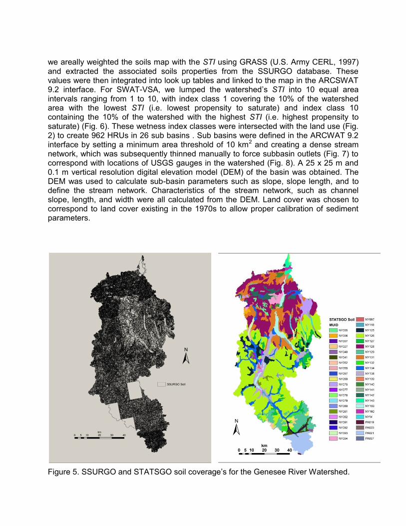
we areally weighted the soils map with the STI using GRASS (U.S. Army CERL, 1997) and extracted the associated soils properties from the SSURGO database. These values were then integrated into look up tables and linked to the map in the ARCSWAT 9.2 interface. For SWAT-VSA, we lumped the watershed‟s STI into 10 equal area intervals ranging from 1 to 10, with index class 1 covering the 10% of the watershed area with the lowest STI (i.e. lowest propensity to saturate) and index class 10 containing the 10% of the watershed with the highest STI (i.e. highest propensity to saturate) (Fig. 6). These wetness index classes were intersected with the land use (Fig. 2) to create 962 HRUs in 26 sub basins . Sub basins were defined in the ARCWAT 9.2 interface by setting a minimum area threshold of 10 km2 and creating a dense stream network, which was subsequently thinned manually to force subbasin outlets (Fig. 7) to correspond with locations of USGS gauges in the watershed (Fig. 8). A 25 x 25 m and 0.1 m vertical resolution digital elevation model (DEM) of the basin was obtained. The DEM was used to calculate sub-basin parameters such as slope, slope length, and to define the stream network. Characteristics of the stream network, such as channel slope, length, and width were all calculated from the DEM. Land cover was chosen to correspond to land cover existing in the 1970s to allow proper calibration of sediment parameters.

Figure 5. SSURGO and STATSGO soil coverage‟s for the Genesee River Watershed.

Figure 6. Wetness Index Classes used in the SWAT-VSA model. The wetness index classes are derived from an areally weighted Soil Topographic Index. SSURGO soil coverage was nested

Required Meteorological Data

Climate data in the form of precipitation, temperature, solar radiation, and humidity are used in the model to predict crop growth, evapotranspiration, and snowmelt. Daily climate data inputs required in the model were precipitation depths, maximum and minimum temperature, solar radiation, wind speed and relative humidity. Meteorological data can be downloaded at: http://www.ncdc.noaa.gov/oa/climate/stationlocator.html.

There are 17 precipitation gages and 9 temperature stations located in the Genesee River Basin that were used in the model. The locations of these stations are shown in the Tables 1 and 2 and Fig. 8.

Table 1. Precipitation Stations

COOP-ID NAME LAT LONG ELEV(m)

300085 ALFRED 42.26083 77.78556 540

300183 ANGELICA 42.30139 77.98917 441

300343 AVON 42.92083 77.75556 166

300443 BATAVIA 43.03028 78.16917 278

300766 BOLIVAR 42.08056 78.17556 482

301974 DANSVILLE 42.56639 77.71833 201

303065 FRIENDSHIP 42.13333 78.23333 500

303722 HASKINVILLE 42.42056 77.56750 503

303773 HEMLOCK 42.78333 77.61667 275

303983 HORNELL 42.35000 77.70000 404

305597 MT MORRIS 42.73056 77.90444 268

306745 PORTAGEVILLE 42.56667 78.05000 356

307167 ROCHESTER 43.11667 77.67667 183

307329 RUSHFORD 42.40000 78.26667 469

308962 WARSAW 42.68333 78.21667 555

309072 WELLSVILLE 42.12194 77.95639 460

309425 WHITESVILLE 42.03833 77.76194 522

Table 2. Temperature Stations

COOP-ID NAME LAT LONG ELEV (m)

300085 ALFRED 42.26083 77.78556 540

300183 ANGELICA 42.30139 77.98917 441

300443 BATAVIA 43.03028 78.16917 278

300766 BOLIVAR 42.08056 78.17556 482

301974 DANSVILLE 42.56639 77.71833 201

303773 HEMLOCK 42.78333 77.61667 275

305597 MT MORRIS 42.73056 77.90444 268

307167 ROCHESTER 43.11667 77.67667 183

308962 WARSAW 42.68333 78.21667 555

Figure 7. Subbasin delineation for the watershed

Precipitation depths and maximum and minimum temperature data was downloaded from NOAA‟s National Climatic Data Center for the period January 1, 1970 through July 31, 2009. Daily datasets were obtained, assembled, and processed for each station to form the SWAT weather input files. Data processing included unit transformation and database file development.

SWAT has the ability to generate values for missing data from a supplied database of weather statistics from stations across the United States. The values for missing data in the downloaded datasets were derived from the statistical information. Daily potential evapotranspiration rates were calculated in the SWAT model using the Penmen-Monteith method. Solar radiation and wind speed were calculated in the model using the weather generator. Meteorological stations were geo-referenced (latitude, longitude, and elevation) and the variables adjusted in SWAT using lapse rates in the watershed.

Streamflow Data

There are 14 stream gages operated by the USGS located within the Genesee River watershed; 12 of these gages monitor flow and 2-monitor stage. Data is available at : http://waterdata.usgs.gov/ny/nwis/ . Figure 8 shows their location in the watershed.

Figure 8. Location of precipitation, temperature, flow, and sediment gauges in the watershed.

http://waterdata.usgs.gov/ny/nwis/

Table 3. Stream Gages in the Genesee River Basin

Sediment Data In April 1975, the USGS began to collect suspended sediment data at seven gauges in the basin. This program continued until September 1977. The data collected was downloaded and used to calibrate the model for sediment. The locations of the sediment monitoring gages are shown in Table 4 and Fig. 8 Table 4. Sediment Gages in the Genesee River Basin

GAUGE WATERWAY HUC LAT LONG

4221000 Genesee River Wellsville 4130002 42.1222 77.9575

4223000 Genesee River Portageville 4130002 42.5703 78.0425

4227500 Genesee River Mt Morris 4130002 42.7667 77.8392

4228500 Genesee River Avon 4130003 42.9178 77.7575

4230500 Oatka Creek Garbutt 4130003 43.0100 77.7917

4227000 Canaseraga Creek Shaker's Crossing 4130002 42.7369 77.8408

4232000 Genesee River Rochester 4130003 43.1806 77.6278

Lakes and Reservoirs There are six major lakes and/or reservoirs within the Genesee River. Four lakes of the Finger Lakes chain are located in the basin. They are Conesus in Subbasin 17, and Hemlock, Canadice, and Honeoye Lakes in Subbasin 16. In addition, two reservoirs were modeled. They are the Mt. Morris Reservoir in Subbasin 22 and the Churchville Reservoir in Subbasin 5. SWAT models lakes and reservoirs based on their proximity to the stream channel. When an impoundment is located along the main stream channel, it is considered as a dam, and when located off-channel it is considered a pond. All of the impoundments modeled in this study are considered as dams. Locations can be seen in Figure 8.

GAUGE WATERWAY HUC LAT LONG YEAR EST. TYPE

4221000 Genesee River Wellsville 4130002 42.1222 77.9575 1956 F

4223000 Genesee River Portageville 4130002 42.5703 78.0425 1902 F

4224775 Canaseraga Creek Above Dansville 4130002 42.5356 77.7044 1972 F

4227500 Genesee River Mount Morris 4130002 42.7667 77.8392 1890 F

4228500 Genesee River Avon 4130003 42.9178 77.7575 1956 F

4229500 Honeoye Creek Honeoye Falls 4130003 42.9572 77.5892 1945 F

4230380 Oatka Creek Warsaw 4130003 42.7442 78.1378 1963 F

4230500 Oatka Creek Garbutt 4130003 43.0100 77.7917 1945 F

4230650 Genesee River Ballantyne Brdg 4130003 43.0922 77.6806 1973 S

4231000 Black Creek Churchville 4130003 43.1006 77.8825 1945 F

4227000 Canaseraga Creek Shaker's Crossing 4130002 42.7369 77.8408 1916 F

4232000 Genesee River Rochester 4130003 43.1806 77.6278 1904 F

4227995 Conesus Creek Lakeville 4130003 42.8556 77.7167 1996 F

4224000 Mt Morris Lake Mt Morris 4130002 42.7333 77.9111 1952 S

. Calibration A two-step procedure was used to calibrate the CNII values for SWAT-VSA‟s wetness index classes based on 1975-1977 data (when corresponding sediment data was available). A basin wide storage (Se) of 16 cm calculated from baseflow separated

runoff plotted against effective precipitation (Pe) used to distribute the e,i values in the basin according to the wetness index (Eq. 9), which results in a basin-wide average CNII = 73 per the method outlined in the model development section (i.e., VSA CNII

method). This first step established the relative distribution of e,i. Because the CN equation is non-linear, the flow predicted using a lumped Se would not necessarily be the same as that predicted as the sum of multiple contributing areas, even if the average storage in both cases is the same. Therefore, we re-ran the calibration uniformly adjusting all the CNII (by CN-units of 0.25) to minimize the RMSE between predicted and measured runoff. The optimized average CNII, over all wetness index classes, was 70, which was similar to that found in an earlier study using SWAT by the US Army Corps of Engineers for the same calibration period, CNII = 70.1. The differential between the CNII value of 73, determined using the VSA methodology described above, and the CNII value of 70, determined using the minimization method, is due to the different runoff calculations used (i.e., Eq. 6 vs. Eq. 7). To insure good calibration, we also made sure that our calibrated result maximized the coefficient of determination (r2) and the Nash-Suttcliffe efficiency (E) (Nash and Suttcliffe, 1970). While the AWC was not „calibrated‟, it was adjusted via Eq. 10 to account for the fact that we recognize that water accumulates in low-lying areas or areas that drain large upslope expanses, and since SWAT does not route water laterally from HRU to HRU, this adjustment was needed to compensate. First order subbasins were calibrated first (i.e.(subbasins #26,25,24,16,5, and 23) followed in increasing order by higher order subbasins (i.e., 20 followed by 18 followed by 10, followed by 13, followed by 2). Parameter sets were not altered after the original calibration. Sediment parameters were calibrated on 1975-1977 data as well. Channel sediment erosion parameters were set to values that allowed the stream channel bed and bank to erode. Upland erosion is modeled using MUSLE. In the MUSLE, the rainfall energy factor is replaced with a runoff factor. This serves to improve the sediment yield prediction, eliminates the need for delivery ratios, and allows the equation to be applied to individual storm events. Sediment yield is improved because runoff is a function of antecedent moisture conditions as well as rainfall energy. Since MUSLE is at best an empirical relationship between physical parameters and erosion, MUSLE sediment parameters were allowed to vary around the tabulated value by 40% during optimization. The calibration objective for flow and sediment was to maximize the NS coefficient while simultaneously trying to minimize the sums of squares error (SSE). The model was calibrated first for flow, then summer sediment load, and then winter sediment load. The baseflow separation technique of Hewlitt and Hibbert (1967) was used to estimate the baseflow component of measured and calibrated model flows at each gauge site.

Subbasins containing no measured flow data were calibrated simultaneously with subbasins containing measured data. For instance subbasins 22, 21, and 19 have no gauge at the outlet, but ultimately drain out of subbasin 18 (Mt Morris), thus they were included in the calibration for the Mt Morris gauge. For sediment calibration, we utilized a parameter transfer methodology from calibrated subbasins. Sediment parameter sets from calibrated subbasins (subbasins 26, 25, 20, 19,18,13, and 2) were transferred to adjacent or otherwise similar (in terms of soil, land use topography) subbasins. For instance sediment parameters from subbasin 25 (Portageville) were transferred to subbasin 23 (Oatka Creek at Warsaw) because they were both adjacent and have similar land use topography and soil properties. Validation We validated SWAT-VSA during the 1977-2009 periods by comparing daily, event and monthly runoff and sediment export predictions to direct measurements. While the model was run on a daily time step, integrated validation was performed on an event basis. For each constituent, model performance was evaluated with four methods: qualitatively using time series plots and quantitatively using the coefficient of determination (r2), the root mean square error (RMSE), and the Nash-Suttcliffe coefficient (NS). Summarized Model Results Streamflow Figures 9-19 show the modeled and SWAT modeled daily streamflow for both the validation period (1975-1977) and validation period. SWAT-VSA simulated streamflow did not differ significantly (p-value<0.05 paired t-test) from measured streamflow at 11 of the 12 gauges. Only modeled streamflow at the gauge on Oatka Creek in Garbutt differed from measured flow (Fig. 14). The difference is mainly a result of over prediction of baseflow. Despite this, the overall streamflow dynamics are well captured, that is predicted runoff peaks generally coincide with measured peaks. No model predictions varied significantly from measured data at the event or monthly time steps. No systematic bias was evident in the results, with predicted vs. observed data evenly scattered around the 1:1 line The largest deviations were generally found during snowmelt or rain on snow events, which are not well captured by SWATs simplistic temperature index snowmelt method, and should warrant father study.

Table 5. Genesee River Basin Flow Calibration Period (1975-1977)

Daily Event Monthly

Site Name Stream Subbasin NS R2

NS R2

NS R2

Wellsville Genesee R. 26 0.67 0.69 0.75 0.71 0.85 0.75

Portageville Genesee R. 25 0.71 0.73 0.79 0.88 0.85 0.87

Mt. Morris Genesee R. 18 0.70 0.73 0.83 0.87 0.91 0.89

Avon Genesee R. 13 0.73 0.74 0.72 0.86 0.82 0.91

Rochester Genesee R. 2 0.74 0.75 0.86 0.82 0.89 0.84

above Dansville Canaseraga Ck. 24 0.64 0.80 0.67 0.80 0.73 0.88

Shaker's Crossing Canaseraga Ck. 20 0.69 0.81 0.67 0.85 0.76 0.89

Warsaw Oatka Ck. 23 0.68 0.72 0.73 0.70 0.86 0.85

Garbutt Oatka Ck. 10 0.52 0.61 0.59 0.68 0.75 0.81

Honeoye Falls Honeoye Ck. 16 0.69 0.70 0.72 0.69 0.79 0.80

Churchville Black Ck. 5 0.71 0.70 0.76 0.74 0.77 0.79

Table 6. Genesee River Basin Flow Validation Period (1977-2009)

Daily Event Monthly


NS R2

NS R2




Avon Genesee R. 13 0.68 0.71 0.72 0.74 0.83 0.87


above Dansville Canaseraga Ck. 24 0.65 0.73 0.69 0.72 0.76 0.80


Warsaw Oatka Ck. 23 0.67 0.70 0.70 0.66 0.83 0.83

Garbutt Oatka Ck. 10 0.58 0.67 0.67 0.73 0.72 0.82

Honeoye Falls Honeoye Ck. 16 0.71 0.68 0.75 0.69 0.76 0.88

Churchville Black Ck. 5 0.66 0.66 0.70 0.70 0.75 0.77

Sediment Figures 9-19 show the modeled and SWAT modeled daily streamflow for both the validation period (1975-1977) and validation period. The model generally predicted daily sediment export form the gauged basins with good levels of accuracy (NS 0.5 to 0.7), somewhat surprising given the limited time scale of the data. Some interesting trends can be observed in the data and model results. For instance, if we are to trust the model predictions to look at long-term sedimentation patterns, the two subbasins on Oatka Creek have rather different results. The first order subbasin (at Warsaw, subbasin 23) has relatively high sediment export, with an average of 166 tons d-1 (Fig. 15). While the

subbasin it drains into (Subbasin 19 at Garbutt) has a comparatively much smaller sediment export (47 tons d-1). This is particularly intriguing considering the difference in the size of the subbasin areas, 104 km2 for Warsaw vs. 423 km2 for Garbutt. This indicates that there is substantial deposition of upstream erosion occurring before Garbutt. This might be the result of the reduced stream power unable to keep sediment entrained as the terrain flattens approaching the Garbutt gauge. Indeed, this is the case, as sediment yield in the Warsaw subbasin was an order of magnitude greater than in the Garbutt subbasin. These types of results point to differing sediment transport mechanisms in different areas of the basin. For instance, there was very little landscape based erosion in the subbasins containing the greater Rochester area. Model results indicated sediment yields from the subbasin of approximately <0.5 ton ha-1, while there was considerable channel or bank erosion (average of approximately 2000 tons d-1). This might be a result of increased runoff from the expanses of impervious surfaces resulting in an increased stream power scouring the more easily erodible loess and fluvial/alluvial deposits in the near lake region. Model results also point to Lower Genesee subbasins having reduced sediment export since the 1970s. The major gauges in the Lower Genesee at Rochester, Avon, Mt Morris, Canasegera Creek at Shakers Crossing, Oatka Creek at Garbutt, and Black Creek at Churchville were all predicted to have decreasing sediment export since the late 1970s. It is not clear what the cause of this reduction is, as there has not been a clear decline in yearly rainfall over that period, but it is a relatively strong trend. This is in contrast to the stable (Canasegera Creek at Dansville) or increasing sediment export (Portageville, Wellsville, Honeoye Falls, Oakta Creek at Warsaw) in Upper Genesee subbasins. Perhaps rainfall patterns within a year are causing the pattern, (e.g., more intense thunderstorms, or reduced snowfall/snow pack). Another potential cause might have been due to several large events in the 1970s, (Hurricane Agnes June 1972 among others), which might have scoured deposited sediment from the Lower Genesee, essentially resetting the system. This would result in increased sedimentation following the event and reduced sediment export. It appears that the discharge at several of the gauges in the Lower Genesee (Rochester, Avon, Mt Morris, and Black Creek at Churchville) has been decreasing as well (Figs 9, 10, 11, and 12), although, again it is unclear why, perhaps increased withdrawals. Intuitively this could be responsible for the reduced sediment export. Conversely, the Upper Genesee gauges do not appear to have experienced reduced discharge, and thus would not be expected to have reduced sediment export.

Table 7. Genesee River Basin Sediment Calibration Period (1975-1977)

Daily Event Monthly


NS R2

NS R2




Avon Genesee R. 13 0.72 0.77 0.74 0.79 0.76 0.81



Garbutt Oatka Ck. 10 0.54 0.69 0.58 0.65 0.65 0.69

Conclusions We modified and developed a SWAT model for the Genesee River Basin in New York State. The model incoporates VSA hydrology in an attempt to better predict runoff and sediment source areas. Observed streamflow at 11 gauges and sediment export at 7 gauges was well captured by the model. Analysis of model data provides insight into mechanisims of erosion and sediment export in the basin. For instance, channel and bank erosion appear to be significant sources of sediment in the Lower Genesee, while both in stream erosion and landscape erosion are important sources in the Upper Genesee subbasins. Thes results and subsequent scenario analysis with the model can help planners and regulatory personell identify important processes in theGenesee Basin and provide support for management decisions. Issues to Consider Due to the size of the basin and the number of HRUs the distributed output of the model at the HRU level were not tested here. The HRU output file is over 9 gigabytes for the entire 40 yr model run, so to effectively utilize these data one would need to run the mode for a shorter time span, or on a longer time step. One of the supposed strengths of the SWAT-VSA methodology is that it better captures the spatial extent of runoff and sediment source areas. This needs to be further tested and validated. The integrated subbasin results appear accurate, and the underlying assumptions of VSA hydrology clearly apply to the majority of the Genesee River Basin, thus we expect the distributed results from SWAT-VSA to be more accurate and underpin better management decisions than results from the standard SWAT model. That being said there is a need for distributed data to test these results, and further refine model methodology. We also feel that it would be worth testing alternative snowmelt/snow accumulation models in the basin, as temperature index method performed poorly.

Figure 9 .

0

200

400

600

800

1000

1200

1972 1974 1976 1978 1980 1982 1984 1986 1988 1990 1992 1994 1996 1998 2000 2002 2004 2006 2008

Dis

char

ge (m

3s-1

)

Observed Flow at Rochester USGS Gauge #4232000

SWAT

Calibration 1975-1977

0

50000

100000

150000

200000

250000

300000

350000

1972 1974 1976 1978 1980 1982 1984 1986 1988 1990 1992 1994 1996 1998 2000 2002 2004 2006 2008

Sed

ime

nt

Exp

ort

(to

n d

-1)

SWAT

Observed Sediment at Rochester USGS Gauge #4232000


Figure 10 .

0

100

200

300

400

500

1972 1974 1976 1978 1980 1982 1984 1986 1988 1990 1992 1994 1996 1998 2000 2002 2004 2006 2008

Dis

cha

rge

(m3

s-1)

Observed Flow at Avon USGS Gauge #4228500

SWAT


0

10000

20000

30000

40000

50000

60000

70000

80000

90000

100000

1972 1974 1976 1978 1980 1982 1984 1986 1988 1990 1992 1994 1996 1998 2000 2002 2004 2006 2008

Sed

imen

t Exp

ort

(to

n d

-1)

SWAT

Observed Sediment at Avon USGS Gauge #4228500


Figure 11.

0

100

200

300

400

500

1972 1974 1976 1978 1980 1982 1984 1986 1988 1990 1992 1994 1996 1998 2000 2002 2004 2006 2008

Dis

cha

rge

(m3

s-1)

Observed Flow at Mt Morris USGS Gauge #4227500

SWAT


0

20000

40000

60000

80000

100000

120000

140000

160000

1972 1974 1976 1978 1980 1982 1984 1986 1988 1990 1992 1994 1996 1998 2000 2002 2004 2006 2008

Sed

imen

t Exp

ort

(to

n d

-1)

Observed Sediment at Mt Morris USGS Gauge #4227500

SWAT


Figure 12.

0

20

40

60

80

100

120

140

160

1972 1974 1976 1978 1980 1982 1984 1986 1988 1990 1992 1994 1996 1998 2000 2002 2004 2006 2008

Dis

char

ge (m

3s-1

)

Observed Flow at Black Creek Churchville USGS Gauge #4231000

SWAT


0

20

40

60

80

100

120

140

160

180

200

1972 1974 1976 1978 1980 1982 1984 1986 1988 1990 1992 1994 1996 1998 2000 2002 2004 2006 2008

Sed

ime

nt

Exp

ort

(to

n d

-1)

SWAT Sediment at Black Creek Churchville USGS Gauge #4231000

Figure 13.

0

20

40

60

80

100

120

140

160

1972 1974 1976 1978 1980 1982 1984 1986 1988 1990 1992 1994 1996 1998 2000 2002 2004 2006 2008

Dis

cha

rge

(m3

s-1)

Observed Flow at Honeoyee Falls USGS Gauge #4229500

SWAT


0

1000

2000

3000

4000

5000

6000

7000

8000

9000

1972 1974 1976 1978 1980 1982 1984 1986 1988 1990 1992 1994 1996 1998 2000 2002 2004 2006 2008

Sed

imen

t Exp

ort

(to

n d

-1)

SWAT Sediment at Honeoyee Falls USGS Gauge #4229500

Figure 14.

0

50

100

150

200

250

1972 1974 1976 1978 1980 1982 1984 1986 1988 1990 1992 1994 1996 1998 2000 2002 2004 2006 2008

Dis

cha

rge

(m3

s-1)

Observed Flow at Oatka Creek Garbutt USGS Gauge #4232500

SWAT


0

500

1000

1500

2000

2500

3000

3500

4000

4500

5000

1972 1974 1976 1978 1980 1982 1984 1986 1988 1990 1992 1994 1996 1998 2000 2002 2004 2006 2008

Sed

ime

nt

Exp

ort

(to

n d

-1)

SWAT

Observed Sediment at Oatka Creek Garbutt USGS Gauge #4232500


Figure 15.

0

10

20

30

40

50

60

70

1972 1974 1976 1978 1980 1982 1984 1986 1988 1990 1992 1994 1996 1998 2000 2002 2004 2006 2008

Dis

char

ge (m

3s-1

)

Observed Flow at Oatka Creek Warsaw USGS Gauge #4230380

SWAT


0

2000

4000

6000

8000

10000

12000

14000

16000

18000

20000

1972 1974 1976 1978 1980 1982 1984 1986 1988 1990 1992 1994 1996 1998 2000 2002 2004 2006 2008

Sed

imen

t Exp

ort

(to

n d

-1)

SWAT Sediment at Oatka Creek Warsaw USGS Gauge #4230380

Figure 16.

0

50

100

150

200

250

300

350

400

1972 1974 1976 1978 1980 1982 1984 1986 1988 1990 1992 1994 1996 1998 2000 2002 2004 2006 2008

Dis

cha

rge

(m3

s-1)

Observed Flow at Canasegera Creek Shakers Crossing USGS Gauge #4227000


0

5000

10000

15000

20000

25000

30000

35000

40000

1972 1974 1976 1978 1980 1982 1984 1986 1988 1990 1992 1994 1996 1998 2000 2002 2004 2006 2008

Sed

imen

t Exp

ort

(to

n d

-1)

SWAT

Observed Sediment at Canasegera Creek Shakers Crossing USGS Gauge #4227000


Figure 17.

0

20

40

60

80

100

120

140

1972 1974 1976 1978 1980 1982 1984 1986 1988 1990 1992 1994 1996 1998 2000 2002 2004 2006 2008

Dis

char

ge (m

3s-1

)

Observed Flow at Canasegera Creek Dansville USGS Gauge #4224775

SWAT


0

2000

4000

6000

8000

10000

12000

14000

16000

18000

20000

1972 1974 1976 1978 1980 1982 1984 1986 1988 1990 1992 1994 1996 1998 2000 2002 2004 2006 2008

Sed

imen

t Exp

ort

(to

n d

-1)

SWAT Sediment at Canasegera Creek Dansville USGS Gauge #42247750

Figure 18.

0

500

1000

1500

2000

2500

1972 1974 1976 1978 1980 1982 1984 1986 1988 1990 1992 1994 1996 1998 2000 2002 2004 2006 2008

Dis

char

ge (m

3s-1

)

Observed Flow at Portageville USGS Gauge #4223000

SWAT


0

100000

200000

300000

400000

500000

600000

700000

1972 1974 1976 1978 1980 1982 1984 1986 1988 1990 1992 1994 1996 1998 2000 2002 2004 2006 2008

Sed

imen

t Exp

ort

(to

n d

-1)

SWAT

Observed Sediment at Portageville USGS Gauge #4223000


Figure 19.

0

50

100

150

200

250

300

350

400

450

1972 1974 1976 1978 1980 1982 1984 1986 1988 1990 1992 1994 1996 1998 2000 2002 2004 2006 2008

Dis

char

ge (m

3s-1

)

Observed Flow at Wellsville USGS Gauge #4221000

SWAT


0

10000

20000

30000

40000

50000

60000

70000

80000

90000

100000

1972 1974 1976 1978 1980 1982 1984 1986 1988 1990 1992 1994 1996 1998 2000 2002 2004 2006 2008

Sed

imen

t Exp

ort

(to

n d

-1)

SWAT


References

Agnew, L.J., S. Lyon, P. Gérard-Marchant, V.B. Collins, A.J. Lembo, T.S. Steenhuis, M.T. Walter. 2006. Identifying hydrologically sensitive areas: Bridging science and application. J. Envir. Mgt. 78: 64-76.

Arnold, J.G., Srinivasan, R., Muttiah, R.R. and Williams, J.R., 1998. Large area hydrologic modeling and assessment part I: model development. J. Am. Water Resour. Assoc., 34(1): 73-89.

Arnold, J.G., and P.M. Allen. 1999. Automated methods for estimating baseflow and ground water recharge from streamflow records. J. Am. Water Resour. Assoc., 35: 411-424.

Beven, K. 2001. Rainfall-Runoff Modeling: The Primer. John Wiley & Sons, LTD. Chichester, England. 360pp.

Beven, K.J. and M.J. Kirkby. 1979. A physically-based, variable contributing area model of basin hydrology. Hydrol. Sci. Bull. 24: 43-69.

Bhaduri, B., J. Harbor, B. Engel, and M. Grove. 2000. Assessing watershed-scale, long-term hydrologic impacts of land-use change using a GIS-NPS model. Environ. Manag. 26:643-658.

Borah, D. K., and M. Bera. 2004. Watershed-scale hydrologic and nonpoint-source pollution models: Review of applications. Trans. ASAE 47:789-803.

Dunne, T. and R.D. Black. 1970. Partial area contributions to storm runoff in a small New England watershed. Water Resour. Res. 6: 1296-1311.

Dunne, T. and L. Leopold. 1978. Water in Environmental Planning. W.H. Freeman & Co., New York. 818pp.

Easton, Z.M., D.R. Fuka, M.T. Walter, D.M. Cowan, E.M. Schneiderman, and T.S. Steenhuis. 2008. Re-conceptualizing the soil and water assessment tool (SWAT) model to predict runoff from variable source areas. J. Hydrol. 348:279– 291.

Franchini, M., and C. Pacciani. 1991. Comparative analysis of several rainfall runoff models. J. Hydrol., 122:161-219.

Haith, D.A. and L.L. Shoemaker. 1987. Generalized Watershed Loading Functions for stream flow nutrients. Water Resour. Bull. 23(3):471-478.

Hewlett, J.D. and A.R. Hibbert. 1967. Factors affecting the response of small watersheds to precipitation in humid regions. In: Forest Hydrology (W.E. Sopper and H.W. Lull, eds.). Pergamon Press, Oxford. pp. 275-290.

Horton, R. E. 1933. The role of infiltration in the hydrological cycle. Trans AGU. 14:446-460.

Johnson, M.S., W.F. Coon, V.K. Mehta, T.S. Steenhuis, E.S. Brooks, and J. Boll. 2003. Application of two hydrologic models with different runoff mechanisms to a hillslope dominated watershed in the northeastern US: a comparison of HSPF and SMR. J. Hydrol. 284:57-76.

Krysanova, V., D. I. Muller-Wohlfeil, and A. Becker. 1998. Development and test of a spatially distributed hydrological water quality model for mesoscale watersheds. Ecol. Model. 106:261-289.

Lyon, S. W., M. T. Walter, P. Gerard-Marchant, and T. S. Steenhuis. 2004. Using a topographic index to distribute variable source area runoff predicted with the SCS curve-number equation. Hydrol. Proc. 18:2757-2771

Nash, J. E., and J. V. Sutcliffe. 1970. River flow forecasting through conceptual models. Part I a discussion of principles. J. Hydrol. 10:282-290.

Page, T., P. M. Haygarth, K. J. Beven, A. Joynes, T. Butler, C. Keeler, J. Freer, P. N. Owens, and G. A. Wood. 2005. Spatial variability of soil phosphorus in relation to the topographic index and critical source areas: Sampling for assessing risk to water quality. J. Environ. Qual. 34:2263-2277.

Qui, Z, M.T. Walter, and C. Hall 2007. Managing variable source pollution in agricultural watersheds. J. Soil Water Conserv., 63(3): 115-122.

Rallison, R.E. 1980. Origin and evolution of the SCS runoff equation. Symposium on Watershed Management. ASCE. New York, NY. pp. 912-924.

Ramanarayanan, T., B. Narasimhan, and R. Srinivasan. 2005. Characterization of fate and transport of isoxaflutole, a soil-applied corn herbicide, in surface water using a watershed model. J. Agric. Food Chem. 53:8848-8858.

Santhi, C., J. G. Arnold, J. R. Williams, L. M. Hauck, and W. A. Dugas. 2001. Application of a watershed model to evaluate management effects on point and nonpoint source pollution. Trans. ASAE 44:1559-1570.

Schneiderman, E.M., T.S. Steenhuis, D.J. Thongs, Z.M. Easton, M.S. Zion, G.F. Mendoza, M.T. Walter, and A.L. Neal. 2007. Incorporating variable source area hydrology into the curve number based Generalized Watershed Loading Function model. Hydrological Processes 21:3420-3430.

Srinivasan, M.S., W.J. Gburek, and J.M. Hamlett. 2002. Dynamics of stormflow generation - A field study in east-central Pennsylvania, USA. Hydrol. Proc., 16(3):649-665.

Srinivasan, M. S., P. Gerard-Marchant, T. L. Veith, W. J. Gburek, and T. S. Steenhuis. 2005. Watershed scale modeling of critical source areas of runoff generation and phosphorus transport. J. Am. Water Resour. Assoc. 41:361-375.

Steenhuis, T. S., M. Winchell, J. Rossing, J. A. Zollweg, and M. F. Walter. 1995. SCS runoff equation revisited for variable-source runoff areas. J. Irrig Drain. Eng. 121:234-238.

Thompson, J. A., E. M. Pena-Yewtukhiw, and J. H. Grove. 2006. Soil-landscape modeling across a physiographic region: Topographic patterns and model transportability. Geoderma 133:57-70.

U.S. Army CERL (1997), GRASS 5.3 users manual, Construction and Engineering Laboratory, Champaign IL.

USDA-NRCS. 2000. Soil Survey Geographic (SSURGO) database for Delaware County, New York, http://www.nrcs.usda.gov/products/datasets/sssurgo/.

USDA-SCS (Soil Conservation Service). 1972. National Engineering Handbook, Part 630 Hydrology, Section 4, Chapter 10.

van Griensven, A., and W. Bauwens. 2003. Concepts for river water quality processes for an integrated river basin modeling. Water Sci. Tech. 48:1-8.

Walter, M.T. and S.B. Shaw. 2005. Discussion: “Curve number hydrology in water quality modeling: Uses, abuses, and future directions” by Garen and Moore. J. Am. Water Resour. Assoc. 41(6): 1491-1492.

Western, A.W., R.B. Grayson, G. Bloschl, G.R. Willgoose, T.A. McMahon. 1999. Observed spatial organization of soil moisture and its relation to terrain indices. Water Resour. Res. 35(3): 797-810.

Williams, J. R., C. A. Jones, and P. T. Dyke. 1984. The EPIC model and its applications. Proc. ICRISAT-IBSNAT-SYSS Symp. on Minimum Data Sets for Agrotechnology Transfer.

http://www.nrcs.usda.gov/products/datasets/sssurgo/

zachary m. easton , daniel r. fuka , tammo s....

Documents