yoon, boung shik (2008) centrifuge modelling of discrete
TRANSCRIPT

CENTRIFUGE MODELLING OF DISCRETE
PILE ROWS TO STABILISE SLOPES
By
Boung Shik Yoon
B.Sc, M.Sc.
Thesis submitted to the University of Nottingham
for the degree of Doctor of Philosophy
November 2008

ii
DECLARATION
I declare that the work in this dissertation was carried out in accordance with the Regulations
of the University of Nottingham. The work is original except indicated by references in the
text and no part of this dissertation has been submitted for any other degree.
_______________________________
Boung Shik, Yoon

iii
ABSTRACT
Discrete pile rows are widely used for improving the stability of potentially unstable slopes,
where columns of reinforced concrete are constructed in the ground to reinforce it and inhibit
instability. The method becomes more cost effective with wider pile spacings, but
simultaneously there is also increasing risk that the soil will flow through the gap between
adjacent piles, rather than arching across it. The impact of pile spacing along the row, which
is likely to have a significant effect on stability, is not clearly understood from a current
design perspective. In this study the effects of pile spacing on passive interaction with the
slope are investigated using a series of geotechnical centrifuge model tests which are
interpreted with a proposed theoretical framework.
A total of 23 geotechnical centrifuge model tests were successfully carried out (Chapters 3
and 4):
• A plane strain model slope was subjected to up to 50 g centrifugal acceleration, with
the upper layer of the slope tending to fail on an underlying predefined surface. The
model piles were instrumented to measure bending moment, and hence the shear
force and pressure on the piles resulting from interaction with the unstable layer
were deduced using a curve-fitting technique. Cameras ‘on-board’ the centrifuge
model allowed in-flight photogrammetry to be used to determine soil or pile
displacement.
• Pile spacing (s/d) was varied, which determined limiting pile-soil interaction for the
row, and variation of other geometrical parameters (l/h) for the slope controlled the
total load on the pile row.
• A number of mechanisms of behaviour for the reinforced slope were identified
ranging from a successfully stabilised slope to shallow and deeper slips passing

iv
through the pile row, as well as slips which occurred upslope of the pile row and
thus did not interact with it.
A theoretical framework was developed and used to interpret the results (Chapter 5):
• The centrifuge model test results have been successfully interpreted using the
proposed analytical approach.
• The centrifuge test results confirm previous numerical modelling results, and hence
a simple theory which can be used for calculation of the maximum stabilising force
available from interaction of the pile row with the slope.
The work presented here also confirmed that another previous theoretical model, although
quite widely used, is somewhat flawed. Comparison with a field study where stabilisation
has been successful (to date) indicated consistency with the experimental results and
associated interpretation.

v
AFFIRMATION
The following publications have been produced during the research for this thesis
Yoon, BS (2008). Centrifuge modelling of discrete piles used for slope stabilisation. The
Young European Arena of Research (YEAR) 2008 for Transport Research Arena (TRA),
nominated as a finalist in a poster section
Yoon, BS & Ellis E.A. (2008). Centrifuge modelling of slope stabilisation using a discrete
pile row. Proceeding of 1st International Conference on Transportation Geotechnics,
Nottingham, UK, 2008. Taylor & Francis Group, London, ISBN 978-0-415-47590-7, pp.
109 – 114.

vi
ACKNOWLEDGEMENTS AND DEDICATION
I wish to express my deepest gratitude to all those who have given great helps and advices
during his research.
First and foremost I would like to show the greatest appreciation to Dr Ed Ellis who always
provided excellent guidance and inspiration whenever need for performing my PhD research.
He has arranged a regular meeting as well as made a room despite of his already busy
schedule for meetings whenever I asked for. He has been more than just a superb supervisor
– Not only has he motivated me to become a professional geotechnical engineer but also
taught me how to sketch my future both in my career and in my life. Again I am sincerely
thankful for the unique honour of working with him, and I also esteem his endless
enthusiasm and endeavour for teach and research. Secondly I wish to acknowledge the
supports provided by Prof. Hai-sui Yu. He has always made great efforts to give all NCG
students (including me) good chances to extend their knowledge on Soil Mechanics.
The opportunity to work with Dr Ed Ellis and Prof. Hai-sui Yu has been the highlight of my
professional career and personal experience in my life.
A special note of recognition and appreciation goes to all technicians of the School of Civil
Engineering, in particular Craig Cox and Mike Langford, who provided the enthusiastic
technical contributions in geotechnical centrifuge modelling.
I am also grateful to the School of Civil Engineering and the University of Nottingham for
financial support that helped me concentrate on the research without financial problems
during the course.
I would like to thank to Professor Heo Yol for his encouragement and to my friends and
colleagues for their friendships and enjoyable discussions.
Finally, I wish to express his sincere gratitude and appreciation to his parents, my wife (Ju-
hee) and my daughter (Ye-jin) for their love and support. I am forever grateful for the many
moments that we enjoyed together in Nottingham.

vii
LIST OF SYMBOLS AND ABBREVIATIONS
English letters
a1, a2 polynomial multipliers in the passive zone
b width of upslope block into page
b0, b1, b2 polynomial multipliers in the active zone
d pile diameter
emax, emin maximum and minimum void ratio of soil
g Earth gravity
h thickness of slip from the surface to the slip plane
l length of upslope block
l/h geometric parameter
n the number of piles across the width b
m the rate of pluviation
p pressure in a pile
pp equivalent pressure on a pile
pp,ult ultimate equivalent pressure on the pile
pr equivalent average pressure per unit width for the pile row
pr = pp (d / s) = Pp / s
ru pore pressure coefficient
s spacing across the pile row
s/d pile spacing (centre to centre)
(s /d )crit critical pile spacing
t thickness of a sand layer deposited by a single pass of the hopper
u pile deflection with depth
vs travel velocity of hopper during pouring

viii
za depth (in the passive zone) measured from the head of the pile
zb depth (in the active zone) measured from the tip of the pile
A = (1 – α) sinβ
where, α = Fμ / Fd
Amax maximum value of A
Bmob normalised lateral interaction stress (= lateral interaction stress on pile /
nominal vertical stress)
Bmax normalised maximum lateral interaction stress (= maximum lateral
interaction stress on pile / nominal vertical stress)
Cu uniformity of coefficient
Cz coefficient of curvature
D10, D30 particle size corresponding to 10% and 30% of particle size distribution
D50 average particle size
EI flexural stiffness of a pile
Fμ resisting force
Fd driving force
G shear modulus of soil
Gs specific gravity
ID relative density of sand
Ka active earth pressure coefficient ( = (1 sin ') / (1 sin ')φ φ− + )
Kp passive earth pressure coefficient (= 1 / Ka)
Ks coefficient of earth pressure on sides
M moment
Mint the bending moment measured at the pre-defined slip interface
N scaling factor or gravity level

ix
Ns, Ts normal and shear forces on the front and back sides in the model
Nb, Tb normal and shear forces on the base in the model
P force acting on the pile per unit length along the axis
Pult net ultimate lateral soil load per unit length of pile
S shear force in a pile
Sp stabilising interaction force on pile (normal load to a pile) equivalent to
the shear force at the sliding interface
Sp,int the total stabilising interaction force on an instrumented pile
W the weight of the upslope block above the pile row (W = lhbγ)
Greek letters
α = Fμ / Fd
β slope angle
δs upslope displacement
δp pile head displacement
δr relative pile-soil displacement
ΔF improvement in the factor of safety
'φ ‘Mohr-Coulomb’ friction angle
'mobφ mobilised angle of shearing ( = sin-1(t / s'))
γ the unit weight of the soil
γd dry density of soil
γw water density
θ gradient (rotation)
μs, μb coefficient of friction on sides and base
ν Poisson’s ratio
x
ρ dry density of soil in model (g / mm3)
ρs,max, ρs,min maximum and minimum dry densities of soil
σ'v effective vertical stress in the model
σ'v0 the nominal vertical effective stress in the soil for a given depth
ψ dilation angle of soil
Abbreviations
PIV Particle Image Velocimetry
BMT Bending Moment Transducer
DAS Data Acquisition System
LB Leighton Buzzard sand
AAE Average Absolute Error
RMSE Root Mean Square Error
FoS Factor of Safety

xi
CONTENTS
Declaration............................................................................................................................... ii
Affirmation .............................................................................................................................. v
Acknowledgements and dedication ........................................................................................ vi
Abstract ................................................................................................................................... iii
List of symbols and abbreviations ......................................................................................... vii
Contents .................................................................................................................................. xi
List of Figures ........................................................................................................................ xv
List of Tables ........................................................................................................................ xxi
CHAPTER 1 INTRODUCTION ......................................................................................... 1
1.1 Research Background .................................................................................................... 1
1.2 Aim and Objectives........................................................................................................ 4
1.3 Layout of the Thesis....................................................................................................... 5
CHAPTER 2 LITERATURE REVIEW ............................................................................. 6
2.1 Introduction.................................................................................................................... 6
2.1.1 General aspects of analysis/ design......................................................................... 6
2.1.2 Structure.................................................................................................................. 8
2.2 Lateral pile-soil interaction ............................................................................................ 9
2.2.1 Elastic Response (isolated pile) .............................................................................. 9
2.2.2 Ultimate Capacity (isolated pile and pile row) ..................................................... 11
2.2.3 Full response (combined elastic and ultimate response)....................................... 14
2.3 Limit equilibrium methods........................................................................................... 18
2.3.1 Slip circle methods................................................................................................ 18
xii
2.4 More complex analytical methods ............................................................................... 22
2.5 Other references ........................................................................................................... 24
2.6 Review of critical factors ............................................................................................. 27
2.6.1 Pile location in slope ............................................................................................. 27
2.6.2 Pile spacing ........................................................................................................... 32
2.6.3 Effect of pile/soil interface roughness .................................................................. 35
2.6.4 Effect of soil dilation ............................................................................................ 36
2.7 Summary ...................................................................................................................... 37
CHAPTER 3 CENTRIFUGE MODELLING: METHODOLOGY ............................... 38
3.1 Introduction.................................................................................................................. 38
3.1.1 Centrifuge modelling: principles and scaling laws ............................................... 38
3.1.2 Structure................................................................................................................ 40
3.2 Test programme ........................................................................................................... 41
3.3 NCG Geotechnical Centrifuge Facilities ..................................................................... 45
3.3.1 NCG Geotechnical centrifuge............................................................................... 45
3.3.2 In-flight digital image processing ......................................................................... 47
3.3.3 Plane strain box..................................................................................................... 50
3.3.4 Sand hoppers......................................................................................................... 51
3.4 Test material: Leighton Buzzard sand ......................................................................... 54
3.4.1 Engineering behaviour of granular soils ............................................................... 54
3.4.2 Test soil property .................................................................................................. 54
3.5 Centrifuge test model ................................................................................................... 57
3.5.1 Model slope........................................................................................................... 57
3.5.3 Model pile ............................................................................................................. 62
3.6 Modelling considerations............................................................................................. 66
3.6.1 Boundary effects ................................................................................................... 66

xiii
3.6.2 Particle size effects................................................................................................ 69
3.6.3 Stress error ............................................................................................................ 70
3.7 Test procedure.............................................................................................................. 72
3.8 Summary ...................................................................................................................... 74
CHAPTER 4 CENTRIFUGE MODELLING: TEST DATA ................................ 75
4.1 Introduction.................................................................................................................. 75
4.1.1 Note on data presentation...................................................................................... 75
4.1.2 Structure of the chapter ......................................................................................... 77
4.2 Ground and pile movement data .................................................................................. 78
4.2.1 Displacements in the cross sectional plane ........................................................... 78
4.2.2 Movement of the slope face .................................................................................. 86
4.2.3 Ground deformation characteristics ...................................................................... 95
4.2.4 Pile head displacements ........................................................................................ 99
4.2.5 Relative pile-soil displacement ........................................................................... 102
4.3 Pile moment data........................................................................................................ 104
4.3.1 Variation of moment with time........................................................................... 104
4.3.2 Moment, shear force, and pressure profiles with depth ...................................... 106
4.3.3 Derived and idealised pile displacements with depth ......................................... 114
4.4 Summary .................................................................................................................... 116
CHAPTER 5 CENTRIFUGE MODELLING: INTERPRETATION AND
COMPARISON ............................................................................................................... 117
5.1 Introduction................................................................................................................ 117
5.2 Theoretical framework for a piled slope .................................................................... 117
5.2.1 Problem definition .............................................................................................. 118

xiv
5.2.2 Stabilising (shear) force ...................................................................................... 121
5.2.3 Pile row interaction ............................................................................................. 123
5.3 Interpretation and comparison ................................................................................... 125
5.3.1 Interpretation of test data .................................................................................... 125
5.3.2 Variation of A and B with g-level in each test .................................................... 127
5.3.3 Variation of A and Bmob with (s/d)....................................................................... 130
5.3.4 Relationship between pile row interaction, (s/d) and (l/h) .................................. 136
5.4 Comparison with previous works .............................................................................. 141
5.4.1 Ito and Matsui (1975).......................................................................................... 142
5.4.2 Chen and Martin (2002); Ang (2005); Durrani (2006) ....................................... 145
5.4.3 Davies et al. (2003) ............................................................................................. 149
5.5 Summary .................................................................................................................... 154
CHAPTER 6 CONCLUSIONS ................................................................................... 157
6.1 Work reported in the thesis ........................................................................................ 157
6.1.1 Centrifuge model tests ........................................................................................ 157
6.1.2 Analytical model ................................................................................................. 159
6.2 Implications for design .............................................................................................. 159
6.3 recommendations for future work.............................................................................. 161
APPENDIX ....................................................................................................................... 163
A. Derivation of pile displacement profile with depth..................................................... 163
REFERENCES ................................................................................................................ 166

xv
LIST OF FIGURES
CHAPTER 1
Figure 1.1 - Slope stabilisation using a discrete bored pile wall: (a) Contribution to
slope stability, and (b) Passive pile-soil-pile interaction ……..........…….
3
CHAPTER 2
Figure 2.1 - Fundamental analysis of pile-soil interaction: (a) Assumed circular
boundary conditions, and (b) Assumed plane strain section …….....……
10
Figure 2.2 - An Idealised piled slope system (after Ito and Matsui, 1975) …......……. 13
Figure 2.3 - ‘Constant overburden’ approach to modelling pile-soil-pile interaction
(after Durrani et al., 2006) …………………………........................…….
15
Figure 2.4 - Conceptual models of an isolated pile and a continuous wall …......……. 16
Figure 2.5 - Ultimate equivalent pressures on a pile row and theoretical limits versus
normalised pile spacing (after Durrani, 2006): (a) Equivalent pressure of
a pile at ‘ultimate’ condition, and (b) Equivalent average pressure ‘along’
the pile row …………………………………................................………
17
Figure 2.6 - Limit equilibrium analyses for a potentially unstable slope stabilised with
pile ………………………………………………………….............……
19
Figure 2.7 - Idealised pile-slope system (after Wang and Yen, 1974) ………......…… 20
Figure 2.8 - Arching development and effect (after Adachi et al., 1987) ….....……… 24
Figure 2.9 - Comparison of the optimal pile location in stabilising a slope:
(a) Optimal location of the pile for a typical slip for comparison,
(b) Optimal location of the pile for a deep seated failure slip in cohesive
soils (after Lee et al., 1995), and (c) Optimal location of the pile for a log
spiral slip (after Ausilio et al., 2003) …………………………………….
29
xvi
Figure 2.10 - Depth of slip measured at crest, midslope, and toe of a slope for a typical
slip ………………………………………………….................…………
30
Figure 2.11 - Effects of pile spacing on the stability of a stabilised slope with the piles:
(a) Improvement ratio versus (s/d) (after Lee et al., 1995),
(b) Factor of safety versus (s/d), and (c) Improvement in FoS versus (s/d)
(after Durrani, 2007) …………………………………..............…………
33
Figure 2.12 - Effect of interface roughness on ultimate equivalent pressure on the pile
…………………………………………………............…………………
35
Figure 2.13 - Effects of soil dilatancy on ultimate resistance and passive interaction … 36
CHAPTER 3
Figure 3.1 - Stress distributions for prototype and centrifuge model
(after Schofield, 1980) ………………………………………......……….
39
Figure 3.2 - Configuration of slope model with a row of piles: (a) Front view, and (b)
Plan view ………………………………………………..................…….
43
Figure 3.3 - Centrifuge testing programme …………………………......……………. 44
Figure 3.4 - NCG centrifuge components ……………………………….....………… 46
Figure 3.5 - Example of PIV analysis used in a test: (a) Initial test mesh, of size 75 ×
75 pixels, (b) Final test mesh and (c) Control point positions, and (d)
Contour plot at 5g ………………………………………..................……
49
Figure 3.6 - Plane strain box components …………………………………….....…… 50
Figure 3.7 - Sand hoppers: (a) Spot type hopper, and (b) Line type hopper .........…… 51
Figure 3.8 - Variation of relative density with thickness of layer for each pass of the
hopper …………………………………………………............…………
53

xvii
Figure 3.9 - Stress analysis of a conventional triaxial test: (a) Mohr circle of effective
stress for a triaxial test, and (b) Derived internal friction angles at peak
and at critical state ………………………………….............................…
56
Figure 3.10 - Schematic arrangement of the test model assuming plane strain
conditions ……………………………………………………......……….
57
Figure 3.11 - Arrangement of the model construction components ……......………….. 58
Figure 3.12 - Test model construction procedures: (a) Stable granular material,
(b) Interface installation, (c) Control points and Latex installation,
(d) Model pile installation, (e) Model without the upper soil layer,
(f) Upper soil layer construction, (g) Upper soil layer without texture,
and (h) Complete upper soil layer with texture ..………...................……
60
Figure 3.13 - Instrumentation of the model pile …………………………......………… 63
Figure 3.14 - Friction angle of interface between soil and pile ……………......………. 65
Figure 3.15 - Cross-section of side boundary lubrication at the edge of the plane strain
section …………………………………………………................………
67
Figure 3.16 - Comparison of friction at lubricated and non-lubricated interfaces:
(a) Modified shear box test, (b) Lubricated boundary interface, and (c)
Non-lubricated boundary interface ………………………...........……….
68
Figure 3.17 - Model dimensions for stress error calculation …………......……………. 70
Figure 3.18 - Vertical stress distributions with depth in the centrifuge model at 50 g
and corresponding prototype …………………….........………………….
71
Figure 3.19 - Complete arrangement of a test package in the centrifuge:
(a) Arrangement of test, and (b) Complete test package on the centrifuge
swing ……………………………………………………..........................
73

xviii
CHAPTER 4
Figure 4.1 - General notation and conventions for position, displacement and loading:
(a) Coordinate system and displacements, and (b) Positive sign
conventions for bending moment, shear force, and pressure ….................
76
Figure 4.2 - Selection of representative examples (BSY12a and BSY15a) …......…… 77
Figure 4.3 - Example of the cross sectional plane view for BSY12a
((s/d) = 2.5, (l/h) = 4.0) ………………………………………......………
81
Figure 4.4 - Contours of downslope movement (mm at model scale) for BSY12a
((s/d) = 2.5, (l/h) = 4.0) …………………………………………......……
82
Figure 4.5 - Examples of the cross sectional plane view for BSY15a
((s/d) = 5.9, (l/h) = 1.5) …………………………………………......……
84
Figure 4.6 - Contours of downslope movement (mm at model scale) for BSY15a
((s/d) = 5.9, (l/h) = 1.5) …………………………………………......……
85
Figure 4.7 - View of the slope face for BSY12a ((s/d) = 2.5, (l/h) = 4.0) …......……... 87
Figure 4.8 - Contour plots of downslope movement (mm, model scale) on the slope
face for BSY12a ((s/d) = 2.5, (l/h) = 4.0) ……………………..................
88
Figure 4.9 - Upslope and downslope displacement (δ) normalised by pile diameter (d)
showing variation with g-level for BSY12a ((s/d) = 2.5, (l/h) = 4.0) ....…
89
Figure 4.10 - View of the slope face for BSY15a ((s/d) = 5.9, (l/h) = 1.5) ………......... 90
Figure 4.11 - Contours of upslope movement (mm, model scale) on the slope face for
BSY15a ((s/d) = 5.9, (l/h) = 1.5) …………………………………............
91
Figure 4.12 - Shallow surface failure ………………………………………………....... 92
Figure 4.13 - Upslope displacement (δu) normalised by pile diameter (d) showing
variation with g-level for BSY12a and 15a …………………………........
93
Figure 4.14 - Upslope displacement (δu) normalised by pile diameter (d) showing
variation with g-level for all tests …………………………………….......
94

xix
Figure 4.15 - Typical characteristics of passive yielding behaviours ………………...... 95
Figure 4.16 - Investigation of arching development between the piles
for BSY12a ………………………………………………………….........
97
Figure 4.17 - Flow action between the piles for BSY15d ((l/h) = 2.5, (s/d) = 8.9) ......... 98
Figure 4.18 - Pile head displacements with g-level for all tests ……………………....... 100
Figure 4.19 - ‘Normalisation’ of pile displacement with g-level for all tests ………...... 101
Figure 4.20 - General definition of relative pile-soil displacement ………………......... 102
Figure 4.21 - Relative pile-soil displacement with g-level …………………………...... 103
Figure 4.22 - Variation of bending moment for BMT 6 (at the interface elevation) with
time …………………………………………………………….................
105
Figure 4.23 - Bending moment, shear force, and lateral pressure
acting on the pile ……………………………………………………........
108
Figure 4.24 - Moment, shear force, and pressure profiles for BSY12a
((s/d) = 2.5, (l/h) = 4.0) ………………………………………………......
112
Figure 4.25 - Moment, shear force, and pressure profiles for BSY15a
((s/d) = 5.9, (l/h) = 1.5) ……………………………………………….......
113
Figure 4.26 - Derived and idealised pile displacement profiles with depth
(BSY12a at 30 g) ……………………………………………………........
115
CHAPTER 5
Figure 5.1 - Idealisation of a piled slope problem for semi-infinite slope ………......... 118
Figure 5.2 - Concepts of limiting interaction capacity for a pile in a row:
(a) Isolated pile, and (b) Continuous wall ……………………………......
124
Figure 5.3 - Variation of A with g-level for all tests ………………………………...... 128
Figure 5.4 - Variation of Bmob with g-level for all tests ………………………….......... 129
Figure 5.5 - Variation of A with various (s/d) for a given (l/h) ………………….......... 133

xx
Figure 5.6 - Variation of Bmob with (s/d) for a given (l/h) …………………………...... 135
Figure 5.7 - Concept of the pile row interaction in terms of A and Bmob …………........ 137
Figure 5.8 - Concept of the pile row interaction in terms of (l/h) and (s/d) ………....... 137
Figure 5.9 - Comparison of test results with the theoretical lines for relative
displacement ………………………………………………………….......
138
Figure 5.10 - Variation of Bmob with relative soil-pile displacement at 50 g showing
results from all tests ………………………………………........................
140
Figure 5.11 - Comparison of ultimate equivalent pressure on pile (Bmob) with (s/d) for
purely frictional soil ( 'φ = 32°) ………………………………….............
144
Figure 5.12 - Boundary conditions of 2d and 3d numerical models used:
(a) Plane strain model (after Chen and Martin, 2002), and
(b) Three-dimensional horizontal slice model (after Ang, 2005) …….......
147
Figure 5.13 - Ultimate equivalent pressures on a pile and on a pile row with theoretical
limits: (a) Ultimate equivalent pile pressure (equivalent to Bmob), and (b)
Equivalent average pressure along the pile row …….................................
148
Figure 5.14 - Geomorphological mapping and schematic layout:
(a) Geomorphological map, (b) Schematic layout of cross-sectional plane
section, and (c) Stabilising force versus improved factor of safety ……...
152
Figure 5.15 - Comparison of Bmob with the ‘factored’ and ‘unfactored’ theoretical
limits ………………………………………………………………….......
153
APPENDIX
Figure A.1 - General definitions and conventions for pile rotation and
displacement .......…………………………………………………………
163

xxi
LIST OF TABLES
CHAPTER 2
Table 2.1 - Summary of references and optimal locations ………………….………... 31
CHAPTER 3
Table 3.1 - Centrifuge model scaling relationships ……………………….………….. 39
Table 3.2 - Centrifuge testing programme ………………………………….……….... 44
Table 3.3 - Centrifuge specification ……………………………………….…………. 46
Table 3.4 - Technical specification of the digital still camera in a test ………...…...... 47
Table 3.5 - Properties of Fraction E Leighton Buzzard sand ……………………..……54
Table 3.6 - Summary of unstable layer and stable material …………….………….…. 61
CHAPTER 4
Table 4.1 - Curve fitting functions used for deriving moment, shear force, pressure
profiles …………………………………………………...………..….…. 109
CHAPTER 5
Table 5.1 - Analysis specification for comparison ……………………..…..….….... 146
Table 5.2 - Geotechnical material properties ……………………………..……….... 149

1
CHAPTER 1
INTRODUCTION
1.1 Research background
Severe instability of slopes involves economic and safety implications for infrastructure such
as roads or railways, damage to other assets located on or adjacent to the potentially unstable
slopes, and potentially even loss of human life. In particular, a significant proportion of UK
transport infrastructure such as embankments or cutting slopes for motorways or railways
may be at risk, due to their age, or from widening projects (Perry et al., 2003a and b).
Climate change with potentially wetter winters and drier summers would pose a further
threat.
A variety of remediation techniques for stabilising a potentially unstable slope exist, for
instance
(1) alteration of the slope geometry to a more stable profile,
(2) installation of drainage to reduce pore water pressure,
(3) insertion of reinforcing inclusions (e.g. retaining walls, piles or geosynthetics)
(4) ground improvement (e.g. grouting or lime mixtures).
The technique of using a single or multiple rows of discrete piles to stabilise potentially
unstable natural or man-made slopes is widely used both in the UK and abroad. The solution
is generally permanent and cost effective, and piles can be situated near the transport
infrastructure (e.g. road or railway line) to provide direct protection to the asset.

CHAPTER 1. INTRODUCTION
2
As shown in Figure 1.1(a) the stabilising piles are installed to penetrate through a sliding soil
mass into stable soil below the slip. Each pile provides horizontal ‘passive’ restraint to the
potentially unstable soil mass, transferring this load down the pile to the underlying stable
ground, where it ‘actively’ resists the load. This results in shear force and bending moments
in the piles, which must have sufficient structural capacity to withstand the loading. Note
that the use of ‘active’ and ‘passive’ in this context does not correspond to earth pressures on
a retaining wall. ‘Passive’ implies that the soil moves relative to the pile and ‘active’ that the
piles moves relative to the soil.
However, the impact of important design factors related to effective performance of the pile
row (e.g. spacing between piles) are not fully understood. The cost effectiveness of the
technique increases as wider pile spacing is used, but simultaneously there is increasing
danger that the soil will ‘flow’ through the gap between piles, rather than arching across it
(Figure 1.1(b) in which arching is a load-transfer mechanism by which stresses from the
yielding parts of the soil mass (potentially unstable soil) are redistributed to the adjoining
non-yielding regions (ultimately the stabilising piles in this case), and hence there is an
improvement in stability of the slope. Arching effects are much greater in sands than in silts
or clays and are greater in dense sands than in loose sands). These uncertainties potentially
lead to conservative and uneconomical design.
The present study focuses on the stabilisation of an inherently unstable slope having a pre-
existing translational slip. This approach allows the pile row interaction and ultimate
resistance for the unstable slope for any frictional soils (e.g. drained behaviour of clay,
although the frictional angle would be lower) to be examined without further complication
regarding the nature of instability through the depth of the slope.

CHAPTER 1. INTRODUCTION
3
(a) Contribution to slope stability
Stabilising pile
Assumed failure surface
Failing soil mass
Passive loading
Active loading
Arching (stress)across the gap
Flow (displacement)between piles
(b) Passive pile-soil-pile interaction
Figure 1.1 - Slope stabilisation using a discrete bored pile wall

CHAPTER 1. INTRODUCTION
4
1.2 Aim and objectives
The general aim of the research is to investigate the behaviour of a piled slope (e.g. pile row
interaction), to give an appraisal on the suitability of a row of discrete piles to stabilise the
slope, and to give fundamental guidance on its design.
The objectives can be specified as:
• to conduct a series of centrifuge model tests on a piled slope
• to examine behaviour of the model by comprehensive analysis of the test data
• to propose a theoretical framework to facilitate interpretation of the results
• to compare the interpreted centrifuge test data with previous work.

CHAPTER 1. INTRODUCTION
5
1.3 Layout of the thesis
Chapter 2 summarises previous studies on the behaviour of piles for slope stabilisation,
ranging from the conventional design method (limit equilibrium approach) to more complex
methods (analytical, empirical and numerical approaches). A review of critical factors
affecting passive interaction is also presented.
Chapter 3 describes the experimental methodology used for centrifuge modelling of a slope
stabilised by a row of piles. The experimental testing programme is first presented, and the
NCG Geotechnical centrifuge facilities such as the centrifuge, model container, model
components and digital image processing techniques are introduced.
Chapter 4 presents an overview of typical centrifuge test data, focusing on profiles of ground
and pile movements (based on image analysis), and pile moment, shear force and pressure
profiles. Preliminary discussion of test results is presented.
Chapter 5 introduces the proposed theoretical framework for interpretation of the results.
The framework is used to present centrifuge test data from all 23 tests, and the results are
compared with selected previous work presented in the literature.
Chapter 6 gives conclusions and suggestions for further work.

6
CHAPTER 2
LITERATURE REVIEW
2.1 Introduction
2.1.1 General aspects of analysis/ design
Most design of piled stabilisation of slopes includes the following aspects (with some
iteration):
1. Evaluation of the total horizontal (or shear) force needed to increase the factor of
safety of the slope by the desired amount
2. Evaluation of the maximum stabilising force available from piles interaction with
potentially unstable material, and comparison with (1)
3. Consideration of other aspects such as
3a. Other slips which do not interact with the piles (e.g. shallow slips upslope or
downslope, or beneath the pile toes)
3b. Whether the piles have sufficient active capacity in the underlying stable soil.
This may also require a check on pile displacement, which will be governed
mainly by active response – however since the calculation is inherently based on
an enhanced factor of safety for the slope displacements may not be considered
meaningful.
3c. Structural design of the piles, based on shear forces and (particularly) bending
moments derived from the passive and active pressure distributions.
CHAPTER 2. LITERATURE REVIEW
7
(1) is normally based on routine slope stability analysis (e.g. method of slices), including the
effect of a horizontal line load representing the total passive restraint from the piles. (3a) is
based purely on slope stability analysis. Since this thesis primarily considers stabilisation of
the slope, established methods of analysis for slope stability will not be considered in detail.
(2) and (3b) are related topics, but since (2) has most direct impact on slope stability it will
be the main focus of this thesis. Since (3c) concerns structural design, it will not be
considered in any detail.
The design will need to consider the following characteristics of the piles:
• the position of the piles in the slope (e.g. near the crest, midslope, or toe)
• the diameter (d) and spacing (s), as well as other structural characteristics
• the length
Practicalities of construction will also impact on these aspects.
The position of the piles in the slope will have some impact on (1) and (2) above, and thus is
likely to be decided at an early stage, mainly based on practicalities of construction and (3a)
(slips occurring upslope or downslope of the piles). Section 2.6 below summarises existing
information in the literature regarding the effectiveness of various locations.
The spacing ratio (s/d) will have a large impact on (2), and this will be the main focus of the
thesis. The pile diameter and type of pile (structural capacity and flexural stiffness) are
mainly related to (3c) and (3b) respectively. The length of the piles is governed by (3a)
(slips passing below the toe of the piles), and (3b).

CHAPTER 2. LITERATURE REVIEW
8
Some authors refer to ‘coupling’ of (1) and (2) above. Generally speaking, the most
straightforward methods consider the various aspects independently (uncoupled), whereas
more complex methods (e.g. 3-d finite element analysis) may claim to completely integrate
(couple) all aspects. However, such approaches are unlikely to be used in routine design.
2.1.2 Structure
It is difficult to categorise all references into well-defined groups. However, in an effort to
structure this the chapter is divided as follows:
• 2.2 Lateral pile-soil interaction (both active and passive)
• 2.3 Limit equilibrium methods
• 2.4 More complex analytical methods
• 2.5 Other references (e.g. lab and field studies)
• 2.6 Review of critical factors
• 2.7 Summary

CHAPTER 2. LITERATURE REVIEW
9
2.2 Lateral pile-soil interaction
Linear elastic and fully plastic (ultimate) responses are initially considered for an ‘isolated’
pile and piles in a row. It is assumed that the ground surface is horizontal (not sloping).
Finally, full response is considered for a row of piles.
2.2.1 Elastic Response (isolated pile)
Baguelin et al. (1977) derived an analytical solution for the lateral reaction of a rigid circular
section (representing the cross section of the pile) displaced through an elastic medium
(representing the soil) with a distant circular boundary about its centre (Figure 2.1(a)). A
plane strain section normal to the axis of the pile was considered (Figure 2.1(b)). The
following solution, based on relative pile-soil displacement in terms of basic elastic soil
parameters, was derived:
1216 (1 ) 2 (3 4 ) ln
(3 4 )p Dv vG d v d
δπ−
⎧ ⎫⎛ ⎞ ⎛ ⎞= − − −⎨ ⎬⎜ ⎟ ⎜ ⎟−⎝ ⎠ ⎝ ⎠⎩ ⎭ (2.1)
where
p = /P d = equivalent pressure acting on the pile section
P = force acting on the pile per unit length along the axis
d = pile diameter
δ = relative pile displacement
G = shear modulus for the elastic medium (soil)
v = Poisson’s ratio of the elastic medium (soil)
D = diameter of circle defining the rigid boundary

CHAPTER 2. LITERATURE REVIEW
10
The value of v can be varied for consideration of drained or undrained loading and soil
properties whereas the value of G is not varied. The value of (D/d) is somewhat arbitrary in
practice, although it must be finite for there to be any resistance to the movement. It is now
known that using a more realistic high stiffness at small strain would reduce this dependency
on far-field effects. A value of 30 has been used by previous researchers to consider an
‘isolated’ pile (i.e. one which is not significantly affected by any neighbouring piles) in
conjunction with the linear elastic response.
Figure 2.1 - Fundamental analysis of pile-soil interaction
Direction of zero strain
Plane strain section
Pile
(b) Assumed plane strain section
Pile
δ
d
Rigid boundary
D
(a) Assumed circular boundary conditions
CHAPTER 2. LITERATURE REVIEW
11
2.2.2 Ultimate Capacity (isolated pile and pile row)
Single (isolated) pile
For granular soils, Broms (1964) suggested an equation deduced from active lateral load
tests on a single pile. It was assumed that ultimate lateral force per unit length is equivalent
to three times the passive earth pressure at all depths.
'ult p v3P K dσ= (2.2)
where,
Pult = net ultimate lateral soil load per unit length of pile
Kp = passive earth pressure coefficient equivalent to )'sin1/()'sin1( φφ −+
'vσ = vertical effective stress
d = pile diameter
Fleming et al. (1994) proposed an empirical equation based on centrifuge test data for a
laterally loaded pile (Barton, 1982) to predict the ultimate lateral load of a single pile. It was
considered that Pult increases in proportion to the square of Kp, giving
2 'ult p vP K dσ= (2.3)
Other authors have proposed variation in proportion to 3pK , and hence Equation (2.3) can be
used as an ‘intermediate’ form of various approaches. Additionally it gives results which are
numerically quite similar to Equation (2.2) for practical values of Kp. Numerical modelling
by Durrani (2006) has also shown this value to be broadly appropriate for limiting
interaction (although potentially slightly high).

CHAPTER 2. LITERATURE REVIEW
12
Pile row
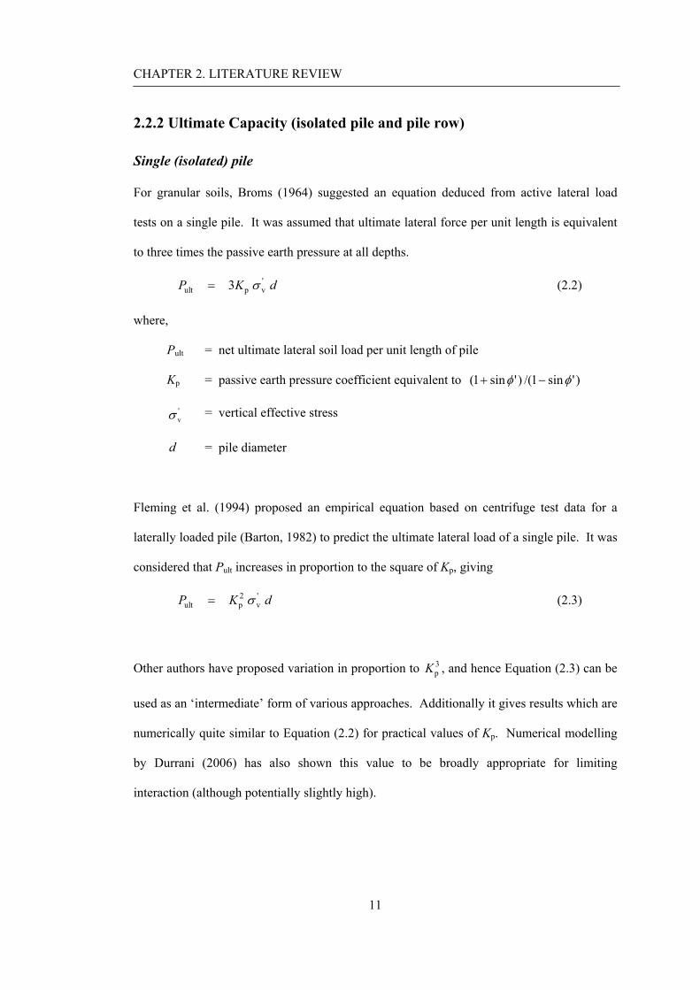
The theory proposed by Ito and Matsui (1975) has been used in a number of publications for
the purpose of calculating the ultimate lateral pressure due to passive pile loading. It was
developed on the basis of a mechanism of plastic deformation of the soil ‘squeezing’
between adjacent piles. Referring to Figure 2.2, a row of piles with diameter (d) at centre-to-
centre spacing (D1) was considered (the ‘clear’ spacing between piles is D2 = D1 - d). The
equivalent lateral pressure acting on a pile (p = P/d) for granular soils is calculated by
Equation (2.4).
1 22
2exp tan tan
8 4D Dzp A N D
N d D φφ
γ π φφ⎧ ⎫⎡ ⎤−⎪ ⎪⎛ ⎞= + −⎨ ⎬⎢ ⎥⎜ ⎟
⎝ ⎠⎪ ⎪⎣ ⎦⎩ ⎭ (2.4)
where
A = 11
2
bDDD
⎛ ⎞⎜ ⎟⎝ ⎠
b = 1/ 2 tan 1N Nφ φφ + −
Nφ = pK = 2tan4 2π φ⎛ ⎞+⎜ ⎟
⎝ ⎠
γ = the unit weight of the soil
φ = the friction angle of the soil
z = depth within the moving layer of soil
CHAPTER 2. LITERATURE REVIEW
13
Figure 2.2 - An Idealised piled slope system (after Ito and Matsui, 1975)
The calculated lateral pressure on the pile(s) tends toward infinity as the pile spacing
becomes a ‘contiguous wall’ (D2 → 0), whilst the lateral pressure approaches zero at very
wide spacings (an ‘isolated single pile’). Both these extremes of behaviour are clearly
unrealistic for passive interaction in a slope. Nevertheless, it has been proposed that the
method is valid for a restricted range of ‘intermediate’ pile spacings (e.g. De Beer and
Carpentier, 1976).
D1
D1 D2
D2 d
d
d
D2 x D1 Direction of deformation
Direction of deformation
x z h
Stabilising pile
Section
Plan
d
Pile
Pile
A
A'
B
B'
⎟⎟⎠
⎞⎜⎜⎝
⎛−
24φπ
⎟⎟⎠
⎞⎜⎜⎝
⎛+
48φπ
⎟⎟⎠
⎞⎜⎜⎝
⎛+=
24φπ
α E
E'

CHAPTER 2. LITERATURE REVIEW
14
2.2.3 Full response (combined elastic and ultimate response)
Liang and Zheng (2002) investigated the soil arching mechanism for ‘drilled shafts’ (piles)
used for slope stabilisation using finite element analysis (PLAXIS). It was reported that the
arching effect reduced as the ratio exceeded three times the pile diameter. Adjacent piles do
no longer interact when the pile spacing is equal to or larger than eight times of the pile
diameter.
Chen and Martin (2002) studied the load-transfer mechanism of stabilising piles using plane
strain numerical analyses (FLAC), focusing on arching development between adjacent piles.
It was reported that tendency of arching becomes stronger as pile spacing get closer whereas
it is likely to be diminished at higher (s/d) in the range 4 to 6. It was also noted that the load
transfer onto the piles is primarily caused by redistribution of the stresses upslope of the piles
with rotation of the principal stress directions.
Durrani et al. (2006) studied pile-soil interaction arising from relative lateral pile-soil
movement, taking account of arching along a pile row in a horizontal section. A translating
pile was used on the basis that there is no fundamental difference between moving a pile
relative to static remote boundaries, and moving remote boundaries relative to a static pile
(e.g. Figure 2.1). (Consideration of a pile row rather than an isolated pile means that
boundaries normal to a line along the row are not remote). The situation was analysed using
a 3-dimensional ‘constant overburden analysis’ (Figure 2.3). This was proposed as an
alternative to a plane-strain analysis, with the stress applied at the upper surface of the
section representing the weight of overlying material. It was found that for a purely
frictional soil strength this gave more rational results than a plane-strain section which had
previously been used by other authors, although the ‘thickness’ of the 3-d section could
influence the results (Durrani et al., 2006).

CHAPTER 2. LITERATURE REVIEW
15
Figure 2.3 - ‘Constant overburden’ approach to modelling pile-soil-pile interaction (after
Durrani et al., 2006)
Figure 2.4 shows conceptual models for the behaviour of
(1) an ‘isolated pile’
(2) a ‘continuous wall’
with corresponding earth pressures in the soil which is passively loading the pile or row, as
proposed by Durrani et al. (2006). The limits are based on Equation 2.3 and active and
passive limits for a retaining wall in level ground respectively.
Figure 2.5(a) shows the equivalent pressure on a pile at ‘ultimate’ conditions, (pp,ult, where
relative pile-soil movement was sufficient to give a maximum interaction pressure),

CHAPTER 2. LITERATURE REVIEW
16
normalised by the ‘constant overburden’ stress (Figure 2.3). Variation with normalised pile
spacing along the row is shown (s = centre-to-centre pile spacing, d = pile diameter).
Equations derived from the conceptual models are also shown (see Chapter 5), and it can be
seen that the data conform quite well to the conceptual models, with behaviour changing
from a continuous wall to an isolated pile as spacing increases. Durrani et al. (2006)
proposed that the intersection of the lines was an approximate limit on arching between
adjacent piles to give an equivalent wall.
Figure 2.5(b) shows an equivalent pressure ‘along’ the pile row, pr = pp (d/s), which is more
relevant to slope stability analysis in a vertical plane strain section. It is now apparent that as
pile spacing increases the ultimate pressure which the row can offer to resist soil movement
reduces, as would be expected.
Figure 2.4 - Conceptual models of an isolated pile and a continuous wall
pK
aK
Isolated pile Continuous wall
2pK

CHAPTER 2. LITERATURE REVIEW
17
0
2
4
6
8
10
12
0 2 4 6 8 10 12
Ulti
mat
e eq
uiva
lent
pile
pre
ssur
e ,p p
,ult
/ σ' v0
s/d
Isolated pile
Continuous wall
(a) Equivalent pressure for a pile at ‘ultimate’ condition
0
10
20
30
40
50
60
70
80
90
1 3 5 7 9 11
Equi
vale
nt a
vera
ge p
ress
ure
alon
g th
e ro
w, p
r(k
N/m
2 )
s/d
Isolated pile
Continuous wall
(b) Equivalent average pressure ‘along’ the pile row
Figure 2.5 - Ultimate equivalent pressures on a pile row and theoretical limits versus
normalised pile spacing (after Durrani, 2006)
Data from numerical analyses

CHAPTER 2. LITERATURE REVIEW
18
2.3 Limit equilibrium methods
Limit equilibrium analyses are widely used in the analysis of stability of earth structures with
or without reinforcing members. They account for the static equilibrium condition of forces
and/or moments developed on potential failure surfaces in the soil. An average factor of
safety along the failure surface is generally calculated by comparing the required shear
strength to maintain a condition of static limit equilibrium with the available shear strength
of the soil.
2.3.1 Slip circle methods
In a slope reinforced with discrete piles a horizontal shear force resulting from soil-structure
interaction is generally assumed to act where the piles intersect with a potential failure slip
(Figure 2.6). The presence of the reinforcing piles in an unstable slope can make a major
contribution to overall stability of the slope by providing an additional resisting force against
sliding.
Slip circle methods for slope stability (normally based on the method of slices) are most
frequently used in design, incorporating the interaction force as a horizontal line load (which
acts on the slip surface which is critical prior to stabilisation). Commercial software
packages for slope stability e.g. SLOPE/W easily allow this approach.
A number of authors (e.g. Lee et al, 1995; Hassiotis et al, 1997; Ausilio et al 2001) have
inherently modified slip circle methods to incorporate the effect of passive interaction above
the slip surface (for instance using Ito & Matsui’s limiting pressure). It is shown (e.g. by
Hassiotis et al, 1997) that inherently considering the stabilising force modifies the critical
slip, and Durrani (2007) demonstrated that logically the critical slip becomes slightly deeper

CHAPTER 2. LITERATURE REVIEW
19
for a given stabilising force. However, for routine design any modification of the slip which
is critical prior to stabilisation is normally ignored.
Figure 2.6 - Limit equilibrium analyses for a potentially unstable slope stabilised with piles
Wang and Yen (1974) assumed that the ‘yielding’ (unstable) layer failed along a potential
failure plane parallel to the slope, and that a row of stabilising piles was embedded in a firm
underlying base (Figure 2.7). The behaviour of the soil was assumed to be rigid-plastic. The
solution proposed two relative spacings (m = B/h), where B is the clear spacing between the
piles and h is the thickness of the unstable layer:
(1) optimum spacing (mm) at which soil arching is likely to be most effective
(2) critical spacing (mcr) beyond which the piles are unlikely to provide any stabilisation.
Stabilising pile
Assumed failure surface
Failing soil mass
Additional force provided by the pile
d
s
s

CHAPTER 2. LITERATURE REVIEW
20
However, three limitations of the theory are apparent:
1. The pile row would behave as a ‘continuous wall’ at narrow spacing. This was not
the ‘most effective’ spacing since arching may be developed even at a wider spacing.
2. The infinite slope assumption might be an ‘oversimplification’ of a complex three-
dimensional problem, most particularly with regard to the upslope and downslope
directions. Additionally, the length of the shear zones (a-a') upslope of the piles is
required to be used in the analysis. Assuming the full upslope length of the slope
can give unrealistic results (Hayward et al., 2000), whilst assumptions for a reduced
length will be arbitrary.
3. The pile diameter was not considered in arching development since only equilibrium
of the soil between the piles was considered.
Figure 2.7 - Idealised pile-slope system (after Wang and Yen, 1974)
φ , c , γ
d
i
x y
a
dx
h
PileYielding layer
Firm layer
1φ , 1c along potential failure plane
Element
B d
P
P+dP
a' b'
b a
A'
A
Dow
nslo
pe d
irect
ion
CHAPTER 2. LITERATURE REVIEW
21
Viggiani (1981) proposed practical solutions to determine the maximum shear force
provided by the pile on the slip surface and the bending moments acting on the pile for the
different failure modes that may occur in practice. The solutions only considered the
ultimate state of purely cohesive soils and the cohesion of the unstable and stable soils were
assumed to be constant with depth. The pile-soil interaction in relation to spacings along the
pile row was not reflected in the solutions.
Some of the conclusions from these references are considered in Section 2.6.
CHAPTER 2. LITERATURE REVIEW
22
2.4 More complex analytical methods
Chen and Poulos (1997) and Poulos (1999) developed methods for computing lateral pile
response based on a specified free-field soil movement profile using a simplified boundary
element analysis or finite difference analysis. The pile was modelled as a simple elastic
beam and the soil as an elastic continuum. It was concluded that a reasonable prediction was
only made when the ratio of soil movement to pile diameter is smaller than about 10%.
Lateral responses rely upon a ‘free field’ soil displacement for the unstable soil (in the
absence of piles) as an input to the analysis, and thus are likely to have limited applicability
in practice.
Jeong et al. (2003) described a simplified numerical approach for analysing the lateral
response of piles in a row. Group interaction factors (representing the effect of pile-soil-pile
interaction) were determined by comparing the maximum bending moment of a pile group
with that of a single pile for a given free-field soil movement in finite element analysis
(ABAQUS). Bishop’s simplified method was used to determine the factor of safety of a
slope without piles and the critical failure surface. The non-linear characteristics of the pile-
soil interaction were modelled by a hyperbolic load transfer curve. The ultimate lateral soil
pressure for a pile in a row was calculated by multiplying the ultimate pressure for a single
pile by the group interaction factor. A computer programme (RSSP) was developed to
perform a series of sequences of the proposed pile-slope stability analysis.
A number of attempts have been made to identify the impact of various design factors
influencing pile-soil interaction in a piled slope based on numerical approaches (e.g. finite
element, finite difference). Examples include Cai and Ugai (2000), Carder and Easton
(2001), Won et al. (2005), Ang (2005) and Durrani et al. (2006). The soil behaviour is
generally assumed to be characterised by an elasto-plastic Mohr-Coulomb failure criterion.
CHAPTER 2. LITERATURE REVIEW
23
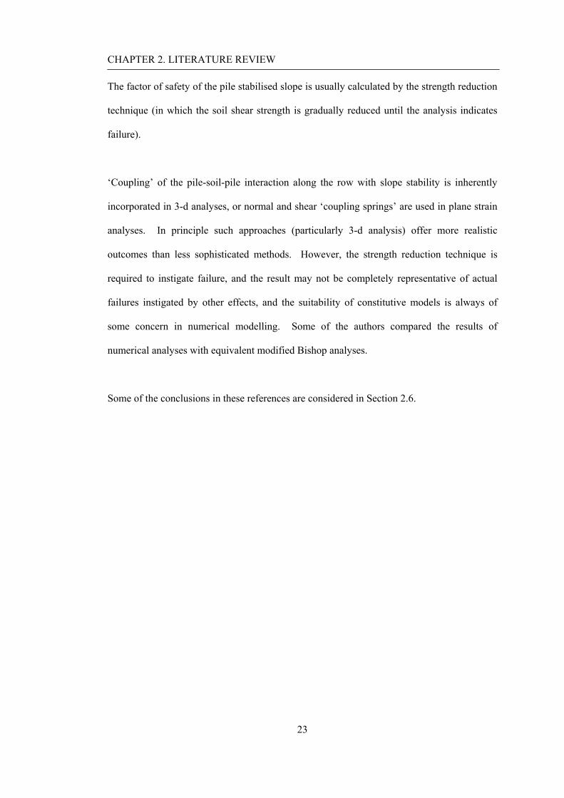
The factor of safety of the pile stabilised slope is usually calculated by the strength reduction
technique (in which the soil shear strength is gradually reduced until the analysis indicates
failure).
‘Coupling’ of the pile-soil-pile interaction along the row with slope stability is inherently
incorporated in 3-d analyses, or normal and shear ‘coupling springs’ are used in plane strain
analyses. In principle such approaches (particularly 3-d analysis) offer more realistic
outcomes than less sophisticated methods. However, the strength reduction technique is
required to instigate failure, and the result may not be completely representative of actual
failures instigated by other effects, and the suitability of constitutive models is always of
some concern in numerical modelling. Some of the authors compared the results of
numerical analyses with equivalent modified Bishop analyses.
Some of the conclusions in these references are considered in Section 2.6.

CHAPTER 2. LITERATURE REVIEW
24
2.5 Other references
Bosscher and Gray (1986) performed reduced-scale model tests in order to investigate the
effect of soil arching in a sandy slope that was restrained by a series of ‘fixed gates’ and
‘swing gates’. The width of the swing gate is analogous to the open spacing between piles.
It was observed that the effect of arching becomes less effective as the swing gate width
increases.
Adachi et al. (1989) attempted to investigate arching phenomenon by examining the
deformation pattern of soil particles (e.g. particle A, B, and C in Figure 2.8) in a series of
model tests using trapdoors. Particles B and C within the arching zone of soil were not
influenced by arching development, as opposed to soil particle A which was. The lateral
pressure is superimposed along the developed arch between the piles and transferred to the
piles. The loads acting on the piles increased with an increase of the pile spacing. However,
the pile behaved like a single pile at (s/d) > 8 (indicating disappearance of any arching
effect).
Figure 2.8 - Arching development and effect (after Adachi et al., 1987)
Load on pile
Drilled shaft
Arching foothold
Soil particle
A
B
C
Equilateral triangular arch
Soil displacement

CHAPTER 2. LITERATURE REVIEW
25
Poulos et al. (1995) and Chen et al. (1997) conducted laboratory model tests on single piles
and pile groups embedded in calcareous sand and subjected to lateral soil movement. The
group effects of the piles were estimated using a dimensionless group factor (the ratio of
ultimate soil pressures for a pile in the group to a single isolated pile). It was reported that
the group effects were diminished when the spacing between the piles exceeded 8 times the
pile diameter.
Hayward et al. (2000) reported a sequence of centrifuge tests on a model cut slope in clay
without or with discrete piles spaced at 3.2, 4.2, and 6.3 diameters. It was concluded that at
a spacing of 3.2 and 4.2 diameters deep seated failure was prevented, but not at a spacing of
6.3 or the unreinforced slope. The limiting lateral pressure on the piles steadily increased as
the pile spacing became larger. A pile spacing of 4 d appeared to be critical for preventing
the slope failure in this case.
The centrifuge test results were compared with other methods for predicting the limiting
lateral pressure. The limiting lateral pressure profile at 6 diameter spacings for a given depth
showed good agreement with the method proposed by Fleming et al. (1994) but the method
proposed by Broms (1964) gave an overestimate. Theoretical methods proposed by Ito and
Matsui (1975) and Wang and Yen (1974) did not give agreement in many respects (e.g. the
relationship of limiting pressure distributions versus pile spacing), indicating that they may
not be suitable for use in analysis.
Carder and Temporal (2000) presented a comprehensive review of the use of spaced piles to
stabilise embankment and cutting slopes. The report reviewed case histories, construction
techniques where soil flow and arching occur, and earlier design methods for stabilising piles.

CHAPTER 2. LITERATURE REVIEW
26
Boeckmann (2006) conducted a series of large scale model tests to study load transfer in
micropiles used to stabilise a sandy slope. Spacing ratios of 5, 10, 15, and 30 diameters were
considered. It was reported that there was a slight tendency for increase in the limiting
lateral pressures with increasing reinforcement spacing ratio. Piles whose head was
restrained against lateral movement showed the greatest limiting pressure as expected.
Thompson and White (2006) performed large scale lateral load tests to verify the use of
drilled and grouted slender piles subject to uniform lateral soil movement. From the results
slender piles may become more cost effective than large diameter piles for particular slope
failure conditions (e.g. shallow failure), considering the mobilised bending moment relative
to maximum bending capacity of the pile. However an increasing danger of structural failure
of the pile and requirement for more piles compared to larger diameter piles should also be
taken into account.
Smethurst and Powrie (2007) presented bending behaviour of discrete piles used to stabilise
a railway embankment at Hildenborough, Kent, UK. The site is underlain by the Weald
Clay to a depth of about 250 m. Piles installed at a spacing of 4 diameters were considered,
and the behaviour over four years after pile installation was monitored. In the short term
there was a significant change in bending moment measured in the piles whilst the longer-
term bending behaviour showed a relatively small subsequent variation. Analysis of the
piles using a simple elastic analysis (using soil displacement measured at the midpoint
between piles, based on the program ALP) was conducted, and showed a reasonable match
to the bending moment and pile displacement measured.
CHAPTER 2. LITERATURE REVIEW
27
2.6 Review of critical factors
Information available from the above references for aspects of analysis of a slope stabilised
by a discrete pile wall are summarised as follows:
• pile row location in the slope
• pile spacing along the row
• effect of the pile-soil interface roughness
• effect of soil dilation
2.6.1 Pile location in slope
Figure 2.9 shows the effect of location (where the pile is most effective in stabilising a slope)
proposed in various references (given in Table 2.1). Here Lx is the horizontal distance from
the toe of the slope to the pile position and L is the horizontal distance from the slope toe to
the crest. Hence for piles at the toe Lx/L = 0 and when the crest is reached Lx/L = 1.
For a typical slip (Figure 2.9(a)) the largest improvement is achieved when the piles are
placed at midslope or near the crest. This is because the depth of the slip below the slope
surface (indicating the depth and hence maximum magnitude of passive interaction) is
similar at the midslope and nearer the crest, but much lower near the toe (Figure 2.10).
However, Lee et al. (1995) argued that for a purely cohesive soil whose strength does not
increase with depth the critical slip tends to become very deep, even passing beneath the pile
tips. The optimal position then becomes at the crest or the toe of the slope because this
failure type readily occurs if the embedded depth of the piles is not sufficient (Figure 2.9(b)
in which the improvement ratio (Nps = Fp/Fs) is the ratio of the improved factor of safety of
the slope with piles (Fp), to the initial factor of safety of the slope without piles (Fs)).

CHAPTER 2. LITERATURE REVIEW
28
However, this finding is specific to analysis using undrained soil strength which does not
increase with depth.
Ausilio et al. (2001) also argued that the critical slip can show increasing tendency to extend
below the base of the slope if a log-spiral curve is used. For this case, the optimal location of
the pile in the slope was then proposed to be between the midslope and toe. However, the
probability of an upslope slip is then increased (Figure 2.9(c) in which K is the stabilising
force normalised by (γH2/2) and η is the improvement ratio in the factor of safety).
Durrani (2007) emphasised two important features of behaviour:
(1) When the piles are near the toe of the slope the depth of interaction (and hence
maximum interaction force) is small, or even zero for a slip occurring upslope of the
pile row.
(2) When the piles are near the crest, although the depth of interaction is quite large less
passive loading was generated, presumably because the mass of soil which is
‘above’ the piles was small.
It is thus plausible that piles at the crest or toe are generally not as effective in stabilising the
slope as at the midslope for a typical slip. These generic observations do not take any
account of the practicality of constructing piles at various locations in the slope, or the
location of infrastructure at the crest or toe of the slope. However, both these factors will
also be of considerable importance in choice of location for actual design scenarios.
Summary of the references considered herein is given in Table 2.1.

CHAPTER 2. LITERATURE REVIEW
29
1
1.2
1.4
1.6
1.8
2
2.2
2.4
2.6
0 0.1 0.2 0.3 0.4 0.5 0.6 0.7 0.8 0.9 1
Fact
or o
f saf
ety,
FoS
Lx / L
Hassiotis et al. (1997) Cai and Ugai (2000): FEM
Cai and Ugai (2000): Bishop Jeong et al. (2003)
Won et al. (2005): FLAC Won et al. (2005): Bishop
Toe of the slope
MidslopeCrest of the slope
(a) Optimal location of the pile for a typical rotational slip for comparison
1
1.04
1.08
1.12
1.16
1.2
0 0.2 0.4 0.6 0.8 1
Impr
ovem
ent r
atio
, Nps
= F
p/ F
s
Lx / L
Toe of the slope
Crest of the slope
Midslope
(b) Optimal location of the pile for a deep seated failure slip in cohesive soils
(after Lee et al., 1995)

CHAPTER 2. LITERATURE REVIEW
30
0
0.05
0.1
0.15
0.2
0.25
0.3
0 0.2 0.4 0.6 0.8 1 1.2
Dim
ensi
onle
ss fo
rce,
K
Lx / L
(c) Optimal location of the pile for a log spiral slip (after Ausilio et al., 2003)
Figure 2.9 - Comparison of the optimal pile location in stabilising a slope
Figure 2.10 - Depth of slip measured at crest, midslope, and toe of a slope for a typical slip
Typical slip: Hassiotis et al. (1997) Cai and Ugai (2000) Carder and Easton (2001) Jeong et al. (2003) Won et al. (2005) Durrani (2007)
Crest
Midslope
Toe
Depth of slip
Deep seated slip: Lee et al. (1995)
Log spiral slip: Ausilio et al. (2003)
η = 1.5
η = 1.3
η = 1.1

31
Table 2.1 - Summary of references and optimal locations
References Method Failure slip type Coupled / Uncoupled
Optimum location
Lee et al. (1995)
Limit equilibrium (for slope stability) Modified boundary element (for pile response prediction)
Deep seated failure slip (even passing beneath of the pile tip)
Uncoupled Crest and toe of a slope
Hassiotis et al. (1998)
Limit equilibrium (for slope stability) Ito and Matsui’s (for ultimate pile pressure prediction)
Typical failure slip Coupled Near the crest of a slope
3d finite element Typical failure slip Coupled (inherently)
Midslope Cai and Ugai
(2000) Modified Bishop’s Typical failure slip Uncoupled Between midslope and the crest
Ausilio et al. (2001)
Limit analysis based on the upper- and lower bound theorems of plasticity
Log-spiral curve type failure slip
Coupled Between midslope and the toe
Carder and Easton (2001)
3d finite element Typical failure slip Coupled (inherently)
Between midslope and the crest
Jeong et al. (2003)
Bishop’s simplified (for slope stability) Finite element (for determining group interaction factors required to calculate the ultimate pressure) Numerical (for pile response prediction)
Typical failure slip Uncoupled Between midslope and the crest
FLAC 3D Typical failure slip Coupled (inherently)
Midslope Won et al.
(2005) Modified Bishop’s (incorporated with Ito and Matsui’s solution for ultimate interaction pressure)
Typical failure slip Uncoupled Near the crest of a slope
Durrani (2007) FLAC 3D (3d constant overburden) Typical failure slip Coupled (inherently)
Midslope
32
2.6.2 Pile spacing
Pile spacing has a significant impact on two important issues:
(1) the improvement in stability of a slope reinforced with piles (considered herein)
(2) passive interaction with respect to development of arching (also previously
considered in Section 2.2.3).
The relationship of the safety factor (FoS) or the improvement ratio (Nps = Fp/Fs) of the slope
with the normalised spacing (s/d) shows that the stability significantly decreases with an
increase of pile spacing (Figure 2.11(a)). This observation seems clearly reasonable –
arching between piles becomes more effective as the pile spacing decreases whereas the
tendency for flow between the piles increases at wider spacing (and hence there is the
reduction in stability).
Figure 2.11(b) also indicates that the pile head condition can influence the factor of safety of
the slope, with a pile which is ‘hinged’ (restrained against horizontal movement at the head)
being more effective than a pile which is ‘free’ (unrestrained) at the head. The piles
considered by Cai & Ugai are tubular, with quite low bending stiffness. Thus the pile
displacement exceeds the soil displacement near the soil surface, giving active rather than
passive loading at the head of the pile. This effect is rather unusual in the context of piles
which are stabilising the slope and reduces the total passive resistance which the flexible
piles offer to a potential slip when horizontal movement is allowed at the head.
Figure 2.11(c) (Durrani, 2007) shows a solid black line for comparison with results from a
series of 3-d ‘constant overburden’ FLAC analyses. The origins of this model of behaviour
are described in Section 5.2.3. Beyond a critical pile spacing (which is postulated to mark
the upper limit of spacing for arching to occur) the improvement in FoS (ΔF) shown by the

33
solid black line reduces as (1/s), and it can be seen that the results show reasonable
agreement with this trend, hence broadly quantifying this effect.
1
1.04
1.08
1.12
1.16
1.2
1 2 3 4 5
Nps
= F
p/ F
s
s/d
Crest pileToe pile
(a) Improvement ratio versus s/d (after Lee et al., 1995)
1
1.2
1.4
1.6
1.8
2
2.2
2.4
2.6
1 2 3 4 5 6 7 8
Fact
or o
f saf
ety,
FoS
s/d
Hassiotis (1997) Cai and Ugai (2000): hingedCai and Ugai (2000): free Jeong et al. (2002) : hingedJeong et al. (2002): free Jeong et al. (2002): BishopWon et al. (2005): fixed Won et al. (2005): freeWon et al. (2005): Bishop
(b) Factor of safety versus s/d

34
0
0.05
0.1
0.15
0.2
0.25
0.3
0.35
0.4
1 2 3 4 5 6 7 8 9 10
Impr
ovem
ent i
n Fo
S, Δ
F
s/d
d = 1.2 m, MSd = 0.3 m, MSd = 0.3 m, US (1/4)d = 0.3 m, DS(1/4)
Midslope pile rows
Upslope and downslope pile rows
Effect of displacementlimit in 3d analyses
(c) Improvement in FoS versus s/d (after Durrani, 2007)
Figure 2.11 - Effects of pile spacing on the stability of a stabilised slope with the piles

35
2.6.3 Effect of pile/soil interface roughness
The effect of pile/soil interface roughness on the ultimate capacity of a pile has been
investigated for a pile spacing of 4 or 5 diameters by Chen and Martin (2002), and Durrani
(2007). The internal friction angle of the granular soil considered was 'φ = 30º. The
ultimate equivalent pressure on the pile is plotted showing variation with the friction angle of
the interface (Figure 2.12). The results show that there is some increase in the ultimate
pressure up to 10˚ but very little effect thereafter. This is probably attributable to the
dominance of difference in normal stresses on the ‘front’ and ‘back’ of the piles rather than
actual shear stress at the interface. The results presented by Chen and Martin (2002) are
inherently lower since they are based on a plane strain analysis rather than the ‘constant
overburden’ approach used by Durrani.
0
1
2
3
4
5
6
7
8
0 5 10 15 20 25 30 35
Ulti
mat
e eq
uiva
lent
pile
pre
ssur
e , p
p,ul
t/ σ
' v0
Interface roughness (φ'int)
Chen and Martin (2002)Durrani (2007)
Figure 2.12 - Effect of interface roughness on ultimate equivalent pressure on the pile

36
2.6.4 Effect of soil dilation
Figure 2.13 shows variation of the ultimate resistance with different dilation angles for
(s/d) = 3, 4, and 5; again showing data from Chen and Martin (2002), and Durrani (2007).
The ultimate resistance is likely to be less affected for a closely spaced pile ((s/d) = 3 in the
analyses by Durrani), when the pile row behaves as a ‘wall’. On the other hand, the higher
dilation angle causes some increase of the ultimate resistance for more widely spaced piles,
which seems reasonable since tendency for volumetric strain will increase the constraint on
soil ‘squeezing’ through the gap between the piles.
0
2
4
6
8
10
12
0 5 10 15 20 25 30 35
Ulti
mat
e eq
uiva
lent
pile
pre
ssur
e , p
p,ul
t/ σ
' v0
Dilation angle, ψ
Chen and Martin (2002): s/d = 4Durrani (2007): s/d = 3Durrani (2007): s/d = 5
s/d = 5, ψ = 0
s/d = 5, ψ= φ'
s/d = 3, ψ = 0
s/d = 3, ψ= φ'
s/d = 4, ψ = 0
s/d = 4, ψ = 15
Figure 2.13 - Effects of soil dilatancy on ultimate resistance and passive interaction

37
2.7 Summary
A number of studies of stabilisation of a slope using piles have been introduced:
• limit equilibrium methods (Section 2.3)
• analytical and/or numerical methods (Section 2.4)
• model or field tests (Section 2.5)
Some of the references have provided a reasonable appraisal of lateral pile-soil interaction
(involving linear elastic and ultimate responses). Many of the design methods presented
have also attempted to provide geotechnical engineers with a generally acceptable prediction
of lateral behaviour of the piles in practical design, but there are still some uncertainties
regarding the impact of critical design factors.
From general observation of critical factors available from the references, the following
conclusions have been drawn:
• The piles are generally most effective somewhere near the mid-height (or crest) of
the slope. However, practical constraints of construction and location of
infrastructure also impact significantly on this aspect of design.
• Arching between piles in a row becomes more effective as the pile spacing decreases
whereas the tendency for flow between the piles increases at wider spacing. Beyond
a critical pile spacing (which is postulated to indicate the upper limit of spacing for
arching to occur), the effect of the piles tends to reduce as (1/s) at wider spacings.
• Pile/soil interface roughness and soil dilation appear to have relatively little effect on
ultimate resistance.

38
CHAPTER 3
CENTRIFUGE MODELLING: METHODOLOGY
3.1 Introduction
3.1.1 Centrifuge modelling: principles and scaling laws
It is widely recognised that reduced scale physical models do not replicate the corresponding
stress regime of a full-scale geotechnical situation. This is a significant problem since the
mechanical behaviour of soil is highly dependent on the magnitude of the current confining
stress (and stress history). Geotechnical centrifuge modelling overcomes this problem and is
the most efficient and robust tool in laboratory simulation for practice and research.
The principle of centrifuge modelling is that the particular full-scale stress regime can be
approximately replicated by increasing centrifugal acceleration to N times Earth’s gravity in
an 1/Nth scale model. This approach works because (for the same soil density) the self-
weight increases by a factor N whilst the length scale is reduced by the same factor so
that σv = γz is correct. Figure 3.1 presents the stress regime in a centrifuge model compared
to that of the equivalent ‘prototype’ (a version of the model which is N times larger).
The scale factors relevant to common geotechnical applications of the centrifuge are given in
Table 3.1. Further details on centrifuge modelling can be found in Schofield (1980) and
Taylor (1995). Errors associated with the inertial stress field are considered in Section 3.6.3.
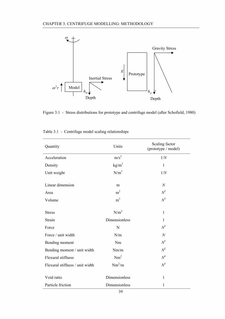
CHAPTER 3. CENTRIFUGE MODELLING: METHODOLOGY
39
Figure 3.1 - Stress distributions for prototype and centrifuge model (after Schofield, 1980)
Table 3.1 - Centrifuge model scaling relationships
Quantity Units Scaling factor (prototype / model)
Acceleration m/s2 1/N
Density kg/m3 1
Unit weight N/m3 1/N Linear dimension m N
Area m2 N2
Volume m3 N3 Stress N/m2 1
Strain Dimensionless 1
Force N N2
Force / unit width N/m N
Bending moment Nm N3
Bending moment / unit width Nm/m N2
Flexural stiffness Nm2 N4
Flexural stiffness / unit width Nm2/m N3 Void ratio Dimensionless 1
Particle friction Dimensionless 1
ω
r2ω Model
Inertial Stress
Depthmh
Prototypeg
Gravity Stress
Depth ph

CHAPTER 3. CENTRIFUGE MODELLING: METHODOLOGY
40
3.1.2 Structure
The Chapter is split into sub-sections as follows:
• 3.2 Centrifuge test programme
• 3.3 NCG Geotechnical Centrifuge facilities
• 3.4 Test material (e.g. engineering properties of the test sand)
• 3.5 Centrifuge test model (e.g. test model and model pile)
• 3.6 Modelling considerations
• 3.7 Test procedure
• 3.8 Summary

CHAPTER 3. CENTRIFUGE MODELLING: METHODOLOGY
41
3.2 Test programme
The centrifuge model was designed to represent an unstable slope in a purely frictional
(granular) soil, inclined at 30° to the horizontal (Figure 3.2). The slope was comprised of a
‘sliding’ (unstable) layer and ‘stable’ underlying material, separated by a prescribed failure
surface. The predefined failure surface was a translational slip plane parallel to the slope
surface at 70 mm depth at model scale. The model piles were installed in a row at discrete
intervals across the slope. The model was assumed to be plane strain (except the pile row,
this will be discussed in Section 3.5.1).
The model is somewhat idealised. The failure interface separating the unstable and stable
material has a very low sliding resistance (see Section 3.6.1), increasing the tendency for the
upper portion of the slope to cause passive loading on the piles over a known depth, so that
this aspect of behaviour could be studied in detail. The model is intended to generically
study this mechanism rather than to represent a specific prototype. It is also worth noting
that design procedures often do not exactly represent real life, and thus idealised generic
approaches such as this can be at least as valuable in informing design as more ‘realistic’
(and hence specific) studies. Likewise, sand has been used, but this is intended to represent
any frictional soil (e.g. drained behaviour of clay, although the friction angle would be
lower).
Selection of the variables was based on combination of the following factors affecting the
pile-soil-pile interaction (Figure 3.2):
(1) the ratio of the upslope length to the thickness of sliding soil ground (l/h) which
essentially controlled the total load on the pile row
(2) the normalised centre to centre pile spacing along the row (s/d) which is a significant
factor in determining limiting pile-soil interaction for the row.

CHAPTER 3. CENTRIFUGE MODELLING: METHODOLOGY
42
Both (1) and (2) (the load on the piles and the limiting capacity) increase nominally in
proportion to g-level. Thus models were subjected to a variety of g-levels (in the range 10 to
50), which is unconventional. The aim was to explore the underlying principles controlling
behaviour rather than consider a specific prototype. The range of g-levels used did however
give soil behaviour considerably more representative of full-scale behaviour (in general) than
a 1-g model. At the maximum acceleration of 50g the 70 mm thick unstable layer
corresponded to 3.5 m.
Initial tests were undertaken to refine the modelling approach. The general arrangement and
components are illustrated in Figure 3.2. Table 3.2 and Figure 3.3 show the tests forming the
final data set reported here.
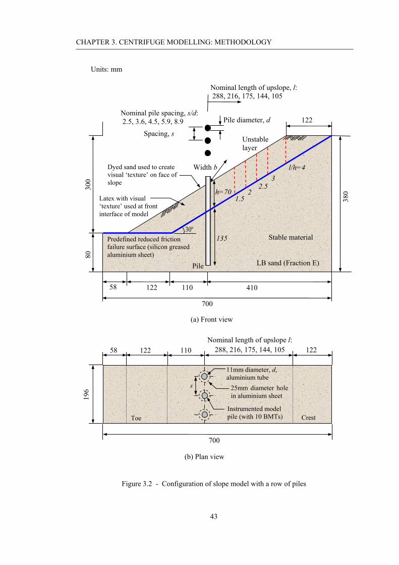
CHAPTER 3. CENTRIFUGE MODELLING: METHODOLOGY
43
Figure 3.2 - Configuration of slope model with a row of piles
700
80
410 122
122
300
Predefined reduced friction failure surface (silicon greased aluminium sheet)
LB sand (Fraction E)
(a) Front view
Dyed sand used to create visual ‘texture’ on face of slope
380
Latex with visual ‘texture’ used at front interface of model
110
30º
58
h=70
Width b l/h=4 3
2 1.5
2.5
Unstable layer
135
Units: mm
Nominal length of upslope, l: 288, 216, 175, 144, 105
Pile
Stable material
Nominal pile spacing, s/d: 2.5, 3.6, 4.5, 5.9, 8.9
Spacing, s
Pile diameter, d
700
58 122 122 Nominal length of upslope l:
288, 216, 175, 144, 105
196
110
11mm diameter, d, aluminium tube
Crest Toe
(b) Plan view
25mm diameter hole in aluminium sheet
Instrumented model pile (with 10 BMTs)
s

CHAPTER 3. CENTRIFUGE MODELLING: METHODOLOGY
44
1
1.5
2
2.5
3
3.5
4
4.5
1 2 3 4 5 6 7 8 9 10
l / h
s/d
12a 15b Boundary of test programme
Test points
13e 15d
15c14b
Figure 3.3 - Centrifuge testing programme
Table 3.2 - Centrifuge testing programme
s/d l/h
2.5 3.6 4.5 5.9 8.9
4 12a 11a 13d 15b -
3 12b 15f 13b 13f -
2.5 14a 14c 13c 13e 15d
2 12c 12d 13a 14g 11c
1.5 14b 14d 15e 15a 15c
Note that boundary values of test programme were designed to cover the general ranges of pile spacing from critical spacing (3 to 4 s/d proposed by Hayward et al. (2000) and Durrani et al. (2006)) to the spacing at which the piles do not interact with the slope (8 s/d proposed by Liang and Zheng (2002)).

CHAPTER 3. CENTRIFUGE MODELLING: METHODOLOGY
45
3.3 NCG geotechnical centrifuge facilities
3.3.1 NCG geotechnical centrifuge
The Nottingham Centre for Geomechanics (NCG) geotechnical centrifuge is a typical
medium-size beam centrifuge with 2.0 m platform radius and a payload capacity of 500 kg at
1.7 m nominal radius up to 100 g. The centrifuge mainly consists of the following
components:
(1) a main body with rotating arms,
(2) a swinging platform (cradle),
(3) counterweight (fixed mass, adjustable position), supplemented by an in-flight
automatic balancing system
(4) electric motor
(5) Data Acquisition System (DAS) cabinets for data transmission
(6) slip rings for transmission of electrical signals and power, and fibre optic rotary joint
for transmission of data
Specification of the NCG geotechnical centrifuge and the components are given in Table 3.3
and Figure 3.4. Specific discussion of NCG centrifuge and DAS can be found in Ellis et al.
(2006).
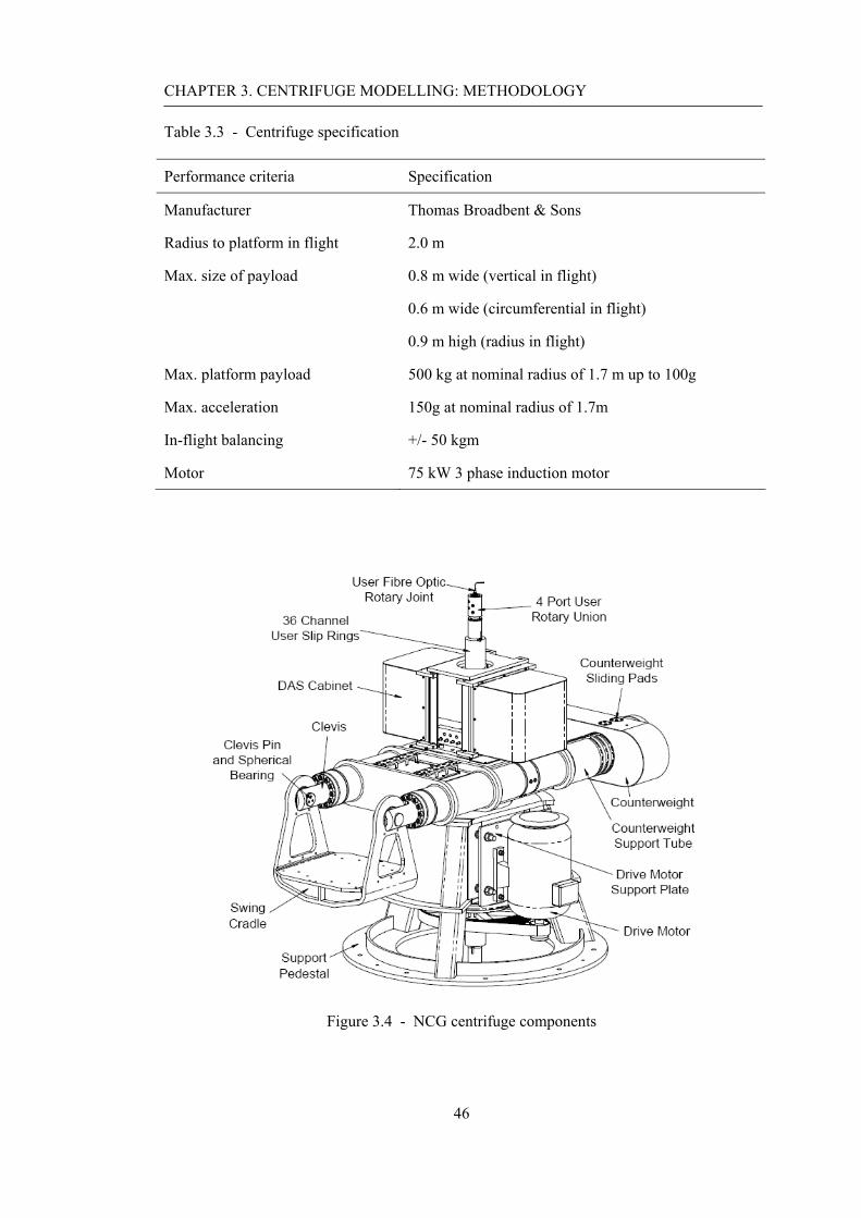
CHAPTER 3. CENTRIFUGE MODELLING: METHODOLOGY
46
Table 3.3 - Centrifuge specification
Performance criteria Specification
Manufacturer Thomas Broadbent & Sons
Radius to platform in flight 2.0 m
Max. size of payload 0.8 m wide (vertical in flight)
0.6 m wide (circumferential in flight)
0.9 m high (radius in flight)
Max. platform payload 500 kg at nominal radius of 1.7 m up to 100g
Max. acceleration 150g at nominal radius of 1.7m
In-flight balancing +/- 50 kgm
Motor 75 kW 3 phase induction motor
Figure 3.4 - NCG centrifuge components

CHAPTER 3. CENTRIFUGE MODELLING: METHODOLOGY
47
3.3.2 In-flight digital image processing
Technical specification
Two digital cameras capable of recording low resolution video and high resolution digital
still images were mounted on the centrifuge swinging platform and the model package. The
technical specification of the digital cameras, and relevant settings used in the tests are
described in Table 3.4. The cameras were controlled in real-time from a PC in the centrifuge
control room using a direct USB connection via the slip rings.
Table 3.4 - Technical specification of the digital still camera in a test
Performance criteria Specification
Camera Model Name Canon PowerShot S70
Dimensions 114 × 57 × 39 mm
Resolution 3072 × 2304 pixels (7.1 megapixels)
Lens 5.8 – 20.7 mm
Focal length 8.6 mm (range: 28 – 100 mm)
Movie clips 640 × 480 pixels
Shooting mode Aperture- priority AE
Shutter speed 1.0 sec (as required to give correct exposure)
Av (Aperture value) 8.0 (chosen to give ‘robust’ focus at g)
Light metering Spot (centre or linked to focusing frame)
Exposure compensation + 2/3
Sensitivity (ISO Speed) ISO 50
AF mode Single AF
Drive mode Single-frame shooting
Other features PC-controlled shooting via USB

CHAPTER 3. CENTRIFUGE MODELLING: METHODOLOGY
48
Artificial visual ‘textures’ consisting of latex sprayed with dots or dyed sand were used on
the front face of the test model and on the exposed slope surface respectively. A sequence of
digital images of these textures was used to infer ground movements using a digital image
processing method based on particle image velocimetry (PIV). The theoretical background
and details of this technique were discussed by White et al. (2003).
PIV analysis procedure
Digital image processing based on PIV was carried out by the following steps:
1. A sequence of digital images was taken during a test.
2. A mesh of test ‘patches’, of size 75× 75 pixels, was generated in the first image to
be analysed (Figure 3.5(a)).
3. A ‘template launch file’ which includes the images to be analysed, analysis
parameters to use, and location of the initial mesh of patches was set up.
4. GeoPIV (programmed in Matlab, and supplied by White et al), tracked the
displacement of test patches for each consecutive image pair and created text files,
see Figure 3.5(b). Texture has been lost over quite a large area of the slope face at
the end of the test due to shallow slope movement. However, more patches could be
tracked earlier in the test, and the upper portion of the slope and the piles can still be
tracked at the end.
5. Unnecessary ‘wild’ (erratic or erroneous) displacement vectors were eliminated.
6. Control point positions (known locations in object space) were defined on the first
image (Figure 3.5(c)).
7. Step (2) – (5) was repeated.
8. Position and movements of the camera during a test were determined using Euler’s
angle formula, focal length, and reference point locations.
9. The programme converted the displacement vectors in image space (pixel
coordinates) into object space (XYZ coordinates)

CHAPTER 3. CENTRIFUGE MODELLING: METHODOLOGY
49
10. Contour plots of the displacement vectors between successive images were
generated and average values of the vectors were displayed (Figure 3.5(d)).
(a) Initial test mesh, of size 75× 75 pixels (b) Final test mesh
(c) Control point positions (d) Contour plot at 5g
Figure 3.5 - Example of PIV analysis used in a test

CHAPTER 3. CENTRIFUGE MODELLING: METHODOLOGY
50
3.3.3 Plane strain box
The model container (internal dimensions: 400 mm high × 200 mm wide × 700 mm long) is
designed to simulate earth structures under plane strain conditions (Figure 3.6). The box has
two end walls and flat base, a back face, and front window. The back face (40 mm thick)
and two vertical side-walls (50 mm thick) of the box are made of aluminium plate with high
stiffness to prevent significant lateral deformation due to earth pressure at high centrifugal
acceleration. The front window is perspex 80 mm thick and allows observation of ground
displacements and failure mechanisms occurring in the soil adjacent to the window.
Figure 3.6 - Plane strain box components
Front window (Transparent Perspex)
Back face (Aluminium plate)
Flat base (Aluminium plate)

CHAPTER 3. CENTRIFUGE MODELLING: METHODOLOGY
51
3.3.4 Sand hoppers
Spot/Line types hoppers
Two types of sand pouring hoppers (‘spot’ and ‘line’), have been developed to construct
centrifuge models at Nottingham (Figure 3.7). The apparatus enables the model soil to be
constructed in a uniform and repeatable manner by means of air pluviation. A range of
densities can be achieved by varying the rate and height of pluviation. The major advantages
of the technique (compared to other methods such as tamping or pouring) are higher dry
density, no particle crushing, less effect of segregation, and better repeatability. The
technique has been verified by Takemura (1998) through cooperative experimental work
undertaken in several centrifuge institutes. It was reported that almost identical dry densities
of sand were achieved by spot and line type hoppers.
(a) Spot type hopper (b) Line type hopper
Figure 3.7 - Sand hoppers

CHAPTER 3. CENTRIFUGE MODELLING: METHODOLOGY
52
Factors controlling dry density
Factors which influence the density of air-pluviated samples are as follows:
(1) the rate of pluviation (m, mass/time), which is controlled by the size and number of
holes at the hopper outlet
(2) travel speed of hopper (vs) during pouring
(3) height of free fall from the hopper to the surface which the soil particles ultimately
land on
It is generally accepted that the density of the resulting model soil reduces as m increases.
Increasing h increases density up to the point where the particles reach their terminal
velocity during free-fall.
The thickness of a sand layer deposited by a single ‘pass’ of the hopper, t, has been derived
by Equation (3.1). This value can be normalised by dividing by the mean particle size d50 of
the soil.
s
mtv bρ
= (3.1)
where,
t = thickness of layer (mm)
m = pouring rate (g/sec)
ρ = dry density of soil in model (g/ mm3)
b = width of deposition for hopper pass (normal to direction of travel) (mm)
vs = travel velocity of hopper (mm/sec)
The relationship between the normalised thickness of a layer (t/d50) and the achievable
relative density ((emax – e)/(emax – emin)) as derived in preliminary tests is shown in Figure 3.8.
The relative density becomes greater as the thickness of the layer decreases, showing a good

CHAPTER 3. CENTRIFUGE MODELLING: METHODOLOGY
53
consistency for all data. This can be logically attributed to the argument that each layer is
compacted by the impact of the subsequent layer, and it is accepted that thin layers are more
readily compacted. The data (except for some of Test 5) was attained at drop height of 0.5 m
for different pouring rates (m) and/or travel velocity of hopper (vs). Some of the data (in Test
5) shows drop height of 1.0 m, which was sufficiently high that there was no increase in
density for increased drop height.
y = -1.0245x + 86.265
0
20
40
60
80
100
0 10 20 30 40 50 60 70
Rel
ativ
e de
nsity
, Id
(%)
Normalised factor (t / d50)
Test1 Test2Test3 Test4Test5
The highest Idat drop height of 1.0 m
All data at drop height of 0.5 m except where indicated
Figure 3.8 - Variation of relative density with thickness of layer for each pass of the hopper.

CHAPTER 3. CENTRIFUGE MODELLING: METHODOLOGY
54
3.4 Test material: Leighton Buzzard sand
3.4.1 Engineering behaviour of granular soils
For granular soils which are not cemented, the strength is often assumed to be entirely
frictional, with zero cohesion intercept. However, the failure envelope of peak strength for a
dense soil usually has some curvature at low mean effective stress due to the transient effect
of dilation which enhances strength. This feature can have significant implications in a
reduced scale model, where confining stresses are small and hence the peak strength of the
soil is unrepresentatively high – the use of centrifuge testing to overcome this has been
discussed above.
3.4.2 Test soil property
Standard classification, particle density and limiting density tests were undertaken according
to BS1377. Details of triaxial testing to determine the strength parameters are given below.
Results are shown in Table 3.5.
Table 3.5 - Properties of Fraction E Leighton Buzzard sand
D10 (mm) D30 (mm) D50 (mm) Cu Cz Gs
0.091 0.105 0.12 1.43 0.93 2.65
ρs,max (kN/m3) ρs,min (kN/m3) emin emax 'peakφ (º) '
critφ (º)
16.27 13.26 0.629 1.004 41 32
Interface properties relevant to the model are reported in Section 3.6.1.

CHAPTER 3. CENTRIFUGE MODELLING: METHODOLOGY
55
A series of drained triaxial tests on LB sand (e = 0.69, Id = 0.84) were conducted to
determine the shear strength of the test soil. The procedure is outlined below:
1. 38mm diameter test specimens were prepared by the dry tamping method in three
sub-layers.
2. The test specimen was saturated under a back pressure of 300 kPa for 2 hours. The
pore pressure coefficient (B) was measured and checked as being at least 95 %.
3. The fully saturated specimen was isotropically consolidated at a given mean
effective pressure of 50, 80, 100, 200, 300 and 400 kN/m2.
4. The sample was sheared under drained condition at a rate of 0.3 mm/min
corresponding to 0.4 %/min, recording relevant data.
In the following stress analysis of a triaxial test, the sand is assumed to be a purely frictional
material with a corresponding failure criterion. The state of stress is represented by drawing
a series of Mohr circles on a (σ' : τ) plot. A mobilised angle of shearing 'mobφ corresponds to
a mobilised stress ratio (τ / σ') during shearing. This is defined by a tangent to the Mohr
circle which passes through the origin and expressed as ( )' 1sin / 'mob t sφ −= where
' '1 3( ) / 2t σ σ= − and ' '
1 3' ( ) / 2s σ σ= + (Figure 3.9(a)). Taking the peak (maximum) and
critical state ratio (τ / σ') during shearing for each test, the peak and critical state angles of
shearing resistance were determined as 'peakφ = 41º and '
critφ = 32º (Figure 3.9(b)).

CHAPTER 3. CENTRIFUGE MODELLING: METHODOLOGY
56
(a) Mohr circle of effective stress for a triaxial test
φ'peak = 41º
φ'crit = 32º
0
100
200
300
400
500
600
700
800
900
0 200 400 600 800 1000 1200 1400
t = (σ
1-σ
3 ) /
2
s' = (σ'1 + σ'3 ) / 2
Best fit of failure envelope at critical state
Best fit of failure evelope at peak
(b) Derived internal friction angles at peak and at critical state
Figure 3.9 - Stress analysis of a conventional triaxial test
'σ
τ
'mobφ
'1σ
'3σ 's
t
O
' '' 1 1 3
' '1 3
sin'mob
ts
σ σφ
σ σ− ⎛ ⎞−⎛ ⎞= = ⎜ ⎟⎜ ⎟ +⎝ ⎠ ⎝ ⎠
Failure envelope

CHAPTER 3. CENTRIFUGE MODELLING: METHODOLOGY
57
3.5 Centrifuge test model
3.5.1 Model slope
Plane strain section
The centrifuge model was designed to simulate the load transfer mechanism arising from
passive interaction on a long row of discrete piles. The plane strain boundaries are required
to be lines of symmetry along the row, and hence were at a location equivalent to the
midpoint between piles in a row extending to either side of the box (Figure 3.10).
Figure 3.10 - Schematic arrangement of the test model assuming plane strain conditions
The model soil was Leighton Buzzard sand (Fraction E) pluviated through air from a line
hopper. The sand is of consistent quality, and has been used extensively for geotechnical
centrifuge testing in the UK. The small particle size was chosen mainly to ensure that
‘Zero strain direction’ (Longitudinal direction)
Row of piles
Pre-defined failure surface
Stable underlying material
Unstable soil layer
Toe of the slope
Crest of the slope
Edges of plane strain section
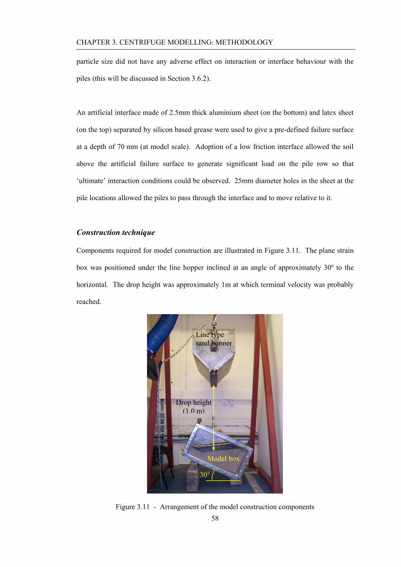
CHAPTER 3. CENTRIFUGE MODELLING: METHODOLOGY
58
particle size did not have any adverse effect on interaction or interface behaviour with the
piles (this will be discussed in Section 3.6.2).
An artificial interface made of 2.5mm thick aluminium sheet (on the bottom) and latex sheet
(on the top) separated by silicon based grease were used to give a pre-defined failure surface
at a depth of 70 mm (at model scale). Adoption of a low friction interface allowed the soil
above the artificial failure surface to generate significant load on the pile row so that
‘ultimate’ interaction conditions could be observed. 25mm diameter holes in the sheet at the
pile locations allowed the piles to pass through the interface and to move relative to it.
Construction technique
Components required for model construction are illustrated in Figure 3.11. The plane strain
box was positioned under the line hopper inclined at an angle of approximately 30º to the
horizontal. The drop height was approximately 1m at which terminal velocity was probably
reached.
Figure 3.11 - Arrangement of the model construction components
Line type sand hopper
Drop height (1.0 m)
Model box
30°
CHAPTER 3. CENTRIFUGE MODELLING: METHODOLOGY
59
Details of model construction are summarised as following:
1. The stable underlying soil (Figure 3.12(a)) was constructed by air pluviation of
sand to a required depth from a constant drop height. The hopper was moved at
approximately constant velocity by swinging it from the gantry.
2. The exact profile of the underlying soil was ‘finished’ by hand to give the required
shape and the ‘failure interface’ was inserted on the underlying soil (Figure 3.12(b)).
3. Latex sheet which had been spray painted to provide visual ‘texture’ (for PIV) was
applied to the front window above the slip plane (Figure 3.12(c)), and similar plain
latex sheet was applied to the back face of the box (see section 3.6.1). The silicone
grease used to lubricate this interface acts to hold the latex on the vertical face
during model construction.
4. Model piles were embedded into the underlying (stable) soil by pushing through the
holes in the failure surface interface (Figures 3.12(d) and (e)).
5. The unstable soil layer was then pluviated onto the interface with pouring rate m =
16 g/sec and travel velocity of hopper vs = 260 mm/s for width b = 198 mm. The
finished slope was trimmed to the desired geometry (Figures 3.12(f) and (g)).
6. Dyed sand was sprinkled over the slope surface to provide PIV texture (Figure
3.12(h)).
The relative density (ID) and the void ratio (e) of the unstable layer and the stable material, as
calculated in each test from the dry density of the resulting models using Gs = 2.64, emax =
1.004, and emin = 0.629 are summarised in Table 3.6. It can be seen that the relative density
was consistently in the range 70 to 80 %.

CHAPTER 3. CENTRIFUGE MODELLING: METHODOLOGY
60
(a) Stable granular material
(b) Interface installation
(c) Control points and Latex installation
(d) Model pile installation
(e) Model without the upper soil layer
(f) Upper soil layer construction
(g) Upper soil layer without texture
(h) Complete upper soil layer with texture
Figure 3.12 - Test model construction procedures

CHAPTER 3. CENTRIFUGE MODELLING: METHODOLOGY
61
Table 3.6 - Summary of unstable layer and stable material
Unstable layer Stable material Test
dγ (kN/m3) e DI (%) dγ (kN/m3) e DI (%)
BSY11A 15.42 0.72 76 15.38 0.72 75
BSY11C 15.38 0.72 75 15.38 0.72 75
BSY12A 15.50 0.71 78 15.33 0.73 73
BSY12B 15.33 0.73 73 15.33 0.73 73
BSY12C 15.38 0.72 75 15.33 0.73 73
BSY12D 15.38 0.72 75 15.33 0.73 73
BSY13A 15.38 0.72 75 15.41 0.72 76
BSY13B 15.50 0.71 78 15.41 0.72 76
BSY13C 15.53 0.71 79 15.41 0.72 76
BSY13D 15.55 0.70 80 15.50 0.71 78
BSY13E 15.53 0.71 79 15.50 0.71 78
BSY13F 15.50 0.71 78 15.50 0.71 78
BSY14A 15.36 0.73 74 15.41 0.72 76
BSY14B 15.26 0.74 71 15.41 0.72 76
BSY14C 15.31 0.73 73 15.41 0.72 76
BSY14D 15.26 0.74 71 15.31 0.73 73
BSY14G 15.41 0.72 76 15.31 0.73 73
BSY15A 15.26 0.74 71 15.36 0.73 74
BSY15B 15.55 0.70 80 15.36 0.73 74
BSY15C 15.26 0.74 71 15.36 0.73 74
BSY15D 15.31 0.73 73 15.53 0.71 79
BSY15E 15.26 0.74 71 15.53 0.71 79
BSY15F 15.50 0.71 78 15.53 0.71 79

CHAPTER 3. CENTRIFUGE MODELLING: METHODOLOGY
62
3.5.3 Model pile
Specification
The model piles were made from 9.53mm outer diameter aluminium tube with 0.914mm
wall thickness (3/8" 20 SWG). Allowing for ‘heat shrink’ later applied to the exterior of the
pile the outer diameter was approximately 11 mm. Their embedded length was 205 mm.
The tube has second moment of inertia 226 mm4. Taking the Young’s Modulus of
aluminium as 70 kN/mm2 this gives a flexural stiffness of 16 MNmm2 = 16 Nm2. Taking an
‘intermediate’ g-level for the tests of 30g, the corresponding prototype diameter and flexural
stiffness are 330 mm and 13 MNm2 respectively. For a solid prototype pile this implies a
Young’s Modulus of approximately 20 GN/m2 – an appropriate value for a cracked concrete
section. The pile diameter is also reasonable since 300 or 450 mm diameter piles would
routinely be used for slope stabilisation.
Pile instrumentation
One of the model piles was instrumented to measure bending moment at 10 locations
through its depth using fully active strain gauge bridges. The gauges were attached to the
exterior of the aluminium tube, and the 0.3mm thick wires also ran up the pile surface. The
positions of the Bending Moment Transducers (BMTs) on the pile are shown in Figure 3.13.
The pile length in the upper sliding layer was 70 mm, with a length of 135 mm in the lower
stable material, making the total embedded length 205 mm.

CHAPTER 3. CENTRIFUGE MODELLING: METHODOLOGY
63
The external instrumentation was protected (against damage during installation and testing)
by epoxy coating and a plastic ‘heat shrink’, which increased the outer diameter of the pile to
approximately 11 mm. The remaining (uninstrumented) model piles were also coated with
heat shrink so that their diameter and surface properties were consistent with the
instrumented pile.
Figure 3.13 - Instrumentation of the model pile
Unit: mm
Nominal position of strain gauges below slope surface: 10, 22, 34, 46, 58, 70, 85, 105, 135, 172.5 mm Sensitive
direction
Solder tabs
Insensitive direction
0.3 mm wire
(b) Strain gauge
Slope surface
Predefined failure plane
12 12 12
12 12
15
20
30
37.5
27.5
70
Sliding direction
135
215
(a) Position of BMTs
45°
5
(c) Closed end
Heat shrink
Wires
BMT

CHAPTER 3. CENTRIFUGE MODELLING: METHODOLOGY
64
BMTs calibration
The instrumented pile BMTs were calibrated using identical signal conditioning to that used
during the test. 10V excitation was supplied to the BMTs and the magnitude of small signals
produced was amplified using a gain of 250 in the signal conditioning. The top end of the
pile was fixed using a clamping block. Small increments of load up to 2.5 kg were applied at
the tip of the pile to cause a known bending moment at each transducer location. Calibration
gave linear voltage output in response to applied bending moment, and hence the calibration
coefficients for specific transducers were derived.
Pile installation
Ideally, model piles should be installed during centrifuge flight by duplicating a field
construction process to give a similar stress regime around the pile. However, this is often
impractical. Furthermore, a number of researchers have demonstrated that the effects of
installation methods and acceleration level at the time of installation for a laterally loaded
pile are less significant than for an axially loaded pile (Craig, 1984; Dyson and Randolph,
1998).
Thus the model piles were initially inserted (driven) into the stable material, and sand was
pluviated around them in the sliding layer at 1 g prior to testing. Spacing between the piles
for each test was carefully measured at the top and near the slip surface to ensure it was
correct.
Pile roughness
As described above, the pile outer diameter consisted of plastic shrink wrap. Pile roughness
can have some effect on lateral interaction with the soil (Lyndon and Pearson, 1988; Chen
and Martin, 2002), tending to make it ‘stiffer’. However, Durrani (2006) showed (based on

CHAPTER 3. CENTRIFUGE MODELLING: METHODOLOGY
65
numerical modelling) that provided the interface friction angle is greater than about 0.3 'φ
there was not significant effect on the ultimate interaction capacity (which consists mainly of
‘bearing’ on the piles rather than sliding at the interface). Interface friction tests between the
shrink wrap and sand (Figure 3.14) indicated that the roughness was comparable to values
for actual piles: precast concrete pile (0.8 – 1.0 'φ ) and rough steel (0.7 – 0.9 'φ ) as
recommended by Kulhawy et al. (1991). Here the interface friction is about 0.75 'φ .
Figure 3.14 - Friction angle of interface between soil and pile
0
10
20
30
40
50
60
70
0 50 100 150
Shea
r str
ess (
kN/m
2 )
Normal stress (kN/m2)
25°
LB sand block (Fraction E)
Aluminium block
Plastic heat shrink

CHAPTER 3. CENTRIFUGE MODELLING: METHODOLOGY
66
3.6 Modelling considerations
3.6.1 Boundary effects
The fundamental assumption of plane strain conditions in centrifuge modelling in principle
requires that there is no friction at the side boundaries (normal to the zero strain direction).
In practice this requires that the friction should be reduced to a practical minimum which
does not have significant effect on the overall response of the model.
Both the unstable layer above the failure surface interface and the stable material below have
contact with the side boundaries of the model container. Since there would be significant
movement of the unstable layer it was important that side friction was minimal here.
However, since the stable material would undergo relatively little movement, and have
considerably less effect on the model in general there was no particular concern regarding
this interface, and no particular precaution was taken to minimise friction here.
However, a latex sheet interface was used to minimise interface friction for the unstable
layer. The latex sheet is directly in contact with the soil and is used to separate it from a
layer of grease trapped between the latex and the inside of the model container (Figure 3.15).
This technique is routinely used in centrifuge testing (Taylor, 1995).
The latex sheet used in the study was sufficiently flexible (having a stiffness of
approximately 1.0 kN/m width) that it would not restrict differential movement of the sand,
which in any case would have tended to move ‘uniformly’ above the failure interface.
However there was likely to be differential movement ‘upslope’ and ‘downslope’ of the pile
row so two separate sheets were used on each face, overlapping but not joined at the pile row
location.
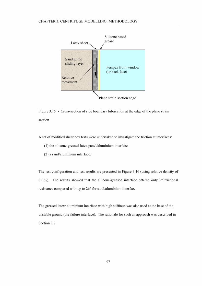
CHAPTER 3. CENTRIFUGE MODELLING: METHODOLOGY
67
Figure 3.15 - Cross-section of side boundary lubrication at the edge of the plane strain
section
A set of modified shear box tests were undertaken to investigate the friction at interfaces:
(1) the silicone-greased latex panel/aluminium interface
(2) a sand/aluminium interface.
The test configuration and test results are presented in Figure 3.16 (using relative density of
82 %). The results showed that the silicone-greased interface offered only 2° frictional
resistance compared with up to 26° for sand/aluminium interface.
The greased latex/ aluminium interface with high stiffness was also used at the base of the
unstable ground (the failure interface). The rationale for such an approach was described in
Section 3.2.
Sand in the sliding layer
Silicone based grease Latex sheet
Perspex front window (or back face)
Plane strain section edge
Relative movement

CHAPTER 3. CENTRIFUGE MODELLING: METHODOLOGY
68
(a) Modified shear box test
0
1
2
3
4
5
6
7
0 50 100 150 200
Shea
r stre
ss (k
N/m
2 )
Normal stress (kN/m2)
2°
(b) Lubricated boundary interface
010203040506070
0 20 40 60 80 100 120 140
Normal stress (kN/m2)
Shea
r stre
ss (k
N/m
2 )
26°
(c) Non-lubricated boundary interface
Figure 3.16 - Comparison of friction at lubricated and non-lubricated interfaces
LB sand block
Aluminium block
LB sand block
Aluminium block
Silicon grease Latex

CHAPTER 3. CENTRIFUGE MODELLING: METHODOLOGY
69
3.6.2 Particle size effects
According to the centrifuge scaling laws, it could be argued that the typical particle size
should be N times smaller in the model than in the prototype. However, it is generally
accepted that the size of soil particles are not reduced in this way. It is more normal to
ensure that the particles are small enough (compared to the other model components) that
individual particle will not affect the continuum behaviour.
Garnier and Konig (1988) proposed that the diameter of a pile must be more than 100 times
the average particle size to minimise any effect on shaft interface behaviour. In a similar
study Foray et al. (1998) concluded that the model pile diameter should exceed 200 times the
average grain size.
However, as noted in Section 3.5.3 lateral pile-soil interaction is more dependent on
‘bearing’ mechanisms than interface behaviour. Equivalent guidance for bearing at the end
of a penetrometer (Gui & Bolton, 1998) requires a pile diameter only 20 times larger than the
particle size.
The diameter of the pile and the smallest pile spacing (= 2.5d) used in the centrifuge tests
was 90 times and 225 times larger than the d50 size of the sand respectively and thus it is
considered extremely unlikely that there would have been any significant impact on
behaviour.
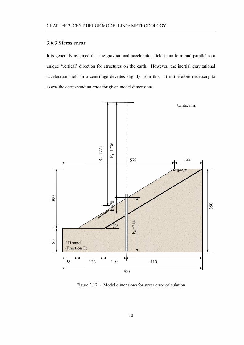
CHAPTER 3. CENTRIFUGE MODELLING: METHODOLOGY
70
3.6.3 Stress error
It is generally assumed that the gravitational acceleration field is uniform and parallel to a
unique ‘vertical’ direction for structures on the earth. However, the inertial gravitational
acceleration field in a centrifuge deviates slightly from this. It is therefore necessary to
assess the corresponding error for given model dimensions.
Figure 3.17 - Model dimensions for stress error calculation
700
58
80
410 122
122 578
300
LB sand (Fraction E)
380
110
30º
h i=7
0 R
t=17
36
h m=2
14
Units: mm R
e=17
71

CHAPTER 3. CENTRIFUGE MODELLING: METHODOLOGY
71
Figure 3.17 shows specific dimensions for this study at the location of the pile row. The
inertial acceleration increases proportionally with radius (depth) in a centrifuge model. Thus
the profile of vertical stress with depth is slightly curved as shown in Figure 3.18 (for a soil
density of 1552 kg/m3, and rotational speed of 16.6 rad/s corresponding to 50 g at a radius of
1.77 m). At the point of maximum under-stress the error compared to the ideal linear
prototype distribution is 1 %. At the failure plane the stress is correct, and at the base of the
model the maximum over-stress is 4 % - however, behaviour at smaller depths is of
considerably more interest. The percentage errors are tolerably small (and independent of g-
level).
The second error of the inertial field is that it always acts in a radial direction, and thus is
inclined to the ‘vertical’ sides of the box. The maximum inclination in these tests is
approximately 10o at the sides, but reducing to zero at the centre of the model (where the
most critical model components are situated).
0
2
4
6
8
10
12
0 50 100 150 200
Dep
th (m
)
Vertical stress (kN/m2)
Model
Prototype
Figure 3.18 - Vertical stress distributions with depth in the centrifuge model at 50g and
corresponding prototype
Equivalent depth of an existing slip plane at 50g
Maximum over-stress
Maximum under-stress

CHAPTER 3. CENTRIFUGE MODELLING: METHODOLOGY
72
3.7 Test procedure
After completing preparation of a test model (as explained above) the test package was
secured to the swinging platform (Figure 3.19), and the instrumentation was connected to the
DAS and checked. Two cameras were also mounted on the swinging platform and on the
test package.
During the test centrifugal acceleration was increased gradually in 1 g increment from 5 g to
16 g. After that, increments of 2 g from 16 g to 30 g, and then 4 g increments from 30 g to
50 g. A sequence of images was taken using the two digital cameras at every gravity
increment.

CHAPTER 3. CENTRIFUGE MODELLING: METHODOLOGY
73
(a) Arrangement of test
(b) Complete test package on the centrifuge swing
Figure 3.19 - Complete arrangement of a test package in the centrifuge
Camera (Front)
Model slope Package
Swing platform
Camera (Top)
Model package
Swing platform
DAS junction
box LightsCamera (Front)
Camera (Top)
Slip rings

CHAPTER 3. CENTRIFUGE MODELLING: METHODOLOGY
74
3.8 Summary
Geotechnical centrifuge modelling is widely recognised to approximately replicate a stress
regime corresponding to an equivalent prototype in laboratory simulation. A centrifuge
model conventionally considers a specific prototype, and is subjected to the relevant scaling
relationship.
The NCG Geotechnical centrifuge is a typical medium-size beam centrifuge with 2.0 m
platform radius and a payload capacity of 500 kg at 1.7 m nominal radius up to 100 g. An
advanced control and data acquisition system, and in-flight digital photography are available.
The centrifuge model used represents an unstable frictional slope that is inclined at 30° to the
horizontal. A prescribed translational slip (with very low resistance) at 70 mm depth (model
scale) was used to generate loading on a pile row. The model piles (3/8'' 20 SWG aluminium
tube) were installed in a row at a discrete intervals across the slope, penetrating through the
unstable layer into stable underlying material. Plane strain was assumed (except for the pile
row). The model soil was Leighton Buzzard Sand (Fraction E), and a silicon-greased
aluminium sheet was used for the slip interface. One model pile was instrumented to
measure bending moment with 10 BMTs along the pile length.
The modelling focused on pile-soil interaction in the unstable ground rather than the slope
stability of a specific prototype. The test programme was therefore established based on
factors affecting this mechanism:
(1) the ratio of the upslope length to the thickness of sliding soil ground (l/h)
(2) the normalised centre to centre pile spacing along the row (s/d).
The centrifuge test results will be presented in Chapter 4.
75
CHAPTER 4
CENTRIFUGE MODELLING: TEST DATA
4.1 Introduction
This chapter presents the centrifuge test data, with some analysis and discussion of the
results. Further discussion and analysis are given in Chapter 5.
4.1.1 Note on data presentation
General
In the present study, the centrifuge test model used focused on investigating the fundamental
understanding of passive stabilisation behaviour rather than considering a specific prototype.
Thus some of the data are discussed based on the centrifuge model at model scale, or in
‘normalised’ terms in order to eliminate scaling effects.
Some of the data is presented either at a specific point in time for a particular g-level, or as a
continuous record of a particular variable with time (and g-level, which varied with time
throughout the test).

CHAPTER 4. CENTRIFUGE MODELLING: TEST DATA
76
Sign conventions
Figure 4.1 shows general sign conventions and notation for position, displacements and
loading in the test. In Figure 4.1(a) positions of test components are denoted using xyz-
coordinates (see Chapter 3), and pile and soil displacements use the u-coordinates (v is the
zero strain direction). Rotation (θ) is positive in the anticlockwise sense.
The convention for bending moment (M), shear force (S), and pressure (p) acting on the pile
are shown in Figure 4.1(b). The sign convention for the bending moment diagram is that
compression on the downslope face of the pile is positive. The pressure is positive when the
net lateral pressure on the pile acts downslope.
(a) Coordinate system and displacements
(b) Positive sign conventions for bending moment, shear force, and pressure
Figure 4.1 - General notation and conventions for position, displacement and loading
z
M S p u
Stable material
z,w
x, u
y, v
θ

CHAPTER 4. CENTRIFUGE MODELLING: TEST DATA
77
4.1.2 Structure of the chapter
Figure 4.2 illustrates the various geometries used in the tests in terms of the length of the
upslope section compared to it’s thickness (l/h) (Figure 3.2) and centre-to-centre pile spacing
compared to the pile diameter (s/d). Table 3.3 also showed this information. Examples
having quite different (l/h) and (s/d) (Figure 4.2) have been selected to provide insight into
the general behaviour of passive loading in sections 4.2 and 4.3:
• 4.2 Ground and pile movement data (based on PIV analysis)
• 4.3 Pile data (based on analysis of moment data and PIV analysis)
• 4.4 Summary
1
1.5
2
2.5
3
3.5
4
4.5
1 2 3 4 5 6 7 8 9 10
l / h
s / d
12a
15a
Boundary of test programme
Tests considered in Section 4.2 and 4.3
Figure 4.2 - Selection of representative examples (BSY12a and BSY15a)

CHAPTER 4. CENTRIFUGE MODELLING: TEST DATA
78
4.2 Ground and pile movement data
In-flight photography and digital imaging processing (based on PIV analysis) were used to
monitor and deduce movements of the unstable soil mass in the cross sectional plane and on
the ‘face’ of the slope during a test. Results from two tests (Figure 4.2) will be considered
below.
4.2.1 Displacements in the cross sectional plane
Displacement profiles of the unstable soil layer in the ‘exposed’ cross sectional plane were
deduced via PIV analysis of latex sprayed with a ‘texture’, as viewed through the transparent
front window of the model at elevated g-level during the test. Separate pieces of latex were
used upslope and downslope of the pile row to allow discontinuity of displacement here if
there was a tendency for this to occur.
A sequence of images for BSY12a ((s/d) = 2.5, and (l/h) = 4.0) were taken from a digital
camera mounted on the swing platform at 1, 10, 20, and 30 g (Figure 4.3). The predefined
failure interface is at 70 mm depth below the surface of the slope at model scale. The
movement of the slope in the plane strain direction is zero at the window interface, which
represents a line of symmetry in terms of pile-soil-pile interaction along the row.
Figure 4.3 shows images taken for processing. The unstable layer is clearly distinguished by
the black latex used at the edge of this layer adjacent to the window (a similar arrangement
was used at the interface with the inside back face of the box). The position of the pile row
is shown by a dotted yellow line.

CHAPTER 4. CENTRIFUGE MODELLING: TEST DATA
79
Without PIV analysis it was hard to identify typical deformation characteristics.
Nevertheless two features can be observed (referring to Figure 4.3(e)): (1) separation of the
upslope and downslope latex panels at the pile row location, and (2) bulging of the toe of the
slope downslope of the pile row. At the end of the test, a ‘passive wedge’ mechanism can be
seen immediately upslope of the pile row as indicated in red – further discussion of this will
be given later.
Figure 4.4 shows a series of contour plots of soil displacement in the downslope direction
derived after PIV analysis, corresponding to the images in Figure 4.3. As anticipated the
unstable soil layer tends to slide downwards along the predefined interface, and significant
soil movements (up to 40 mm) are observed downslope of the piles. Movement upslope of
the piles is considerably restrained by the pile row.
A ‘passive wedge’ developed above the pile row can be identified in the PIV analysis
(Figure 4.4(c)). Displacement of the soil immediately behind the pile row is relatively small,
but it is higher at the crest. This implies two aspects of behaviour:
1. Restraint of soil immediately behind the pile row. Since the soil is loading the pile
row there is analogy with a ‘passive wedge’
2. Increasing possibility of a potential slip upslope of the passive wedge which does not
interact with the pile row
The upward bulge immediately behind the pile row in Figure 4.3(e) supports both these
hypotheses, and the mechanisms potentially ‘interact’ since the bulge could either be
attributed to the passive wedge, or a ‘toe bulge’ for the upslope mechanism.
This kind of failure mechanism tended to develop with an increase of (l/h) for a given (s/d)
and decrease of (s/d) for a given (l/h). The former increases the probability of a mechanism

CHAPTER 4. CENTRIFUGE MODELLING: TEST DATA
80
upslope of the piles, whilst the latter implies greater resistance from the pile row
corresponding to the passive wedge loading the row.

CHAPTER 4. CENTRIFUGE MODELLING: TEST DATA
81
(a) 1 g (b) 10 g
(c) 20 g (d) 30 g
(e) Typical deformation characteristics (taken at 50 g)
Figure 4.3 - Example of the cross sectional plane view for BSY12a ((s/d) = 2.5, (l/h) = 4.0)
Passive wedge block may be observed upslope of the pile
Sliding direction
Upslope
Downslope
Separation of side lubrication
Bulging with transverse cracks
Position of pile row
Underlying stable material

CHAPTER 4. CENTRIFUGE MODELLING: TEST DATA
82
0 50 100 150 200 250 300 350 400 450 500
0
50
100
150
200
2502
3
4
5
6
7
8
9
10
(a) 1 to 10 g
0 50 100 150 200 250 300 350 400 450 500
0
50
100
150
200
250 5
10
15
20
25
30
(b) 1 to 20 g
0 50 100 150 200 250 300 350 400 450 500
0
50
100
150
200
250 10
15
20
25
30
35
40
(c) 1 to 30 g
Figure 4.4 - Contours of downslope movement (mm at model scale) for BSY12a ((s/d) =
2.5, (l/h) = 4.0)
Passive wedge failure
Transverse bulging
Pile
Crest
Toe
Crest
Toe
Pile
Crest
Toe
Pile

CHAPTER 4. CENTRIFUGE MODELLING: TEST DATA
83
Figure 4.5 and Figure 4.6 show equivalent images and contours for BSY15a ((s/d) = 5.9,
(l/h) = 1.5). Note that the unstable layer does not extend to the top of the interface since (l/h)
= 1.5 < 4. In fact the latex panel extends beyond the top of the unstable sand layer, and thus
it misleadingly appears that (l/h) is somewhat greater than 1.5. The results are generally
similar to BSY12a, except that there is no significant evidence of a ‘passive wedge’ upslope
of the pile row at 30g.
Figure 4.6 illustrates the upslope movement derived from images taken in the cross sectional
plane with increase of g-level. Generally speaking the upslope displacement tends to
increase with (s/d) for a given (l/h), and for a given (s/d) displacement tends to increase with
(l/h). This is a reasonable trend of behaviour, as would be anticipated.
In summary, the ground movements in the cross sectional plane are satisfactorily deduced
using digital image processing (PIV analysis) on a series of images taken during a test,
including some important features of ground deformation.

CHAPTER 4. CENTRIFUGE MODELLING: TEST DATA
84
(a) 1 g (b) 10 g
(c) 20 g (d) 30 g
Figure 4.5 - Examples of the cross sectional plane view for BSY15a ((s/d) = 5.9, (l/h) = 1.5)

CHAPTER 4. CENTRIFUGE MODELLING: TEST DATA
85
100 150 200 250 300 350
100
120
140
160
180
200
220
240
260
2
3
4
5
6
7
8
9
10
11
12
(a) 1 to 10 g
100 150 200 250 300 350
100
120
140
160
180
200
220
240
260
5
10
15
20
25
30
35
(b) 1 to 20 g
100 150 200 250 300 350
100
120
140
160
180
200
220
240
260 5
10
15
20
25
30
35
40
45
(c) 1 to 30 g
Figure 4.6 - Contours of downslope movement (mm at model scale) for BSY15a ((s/d) =
5.9, (l/h) = 1.5)

CHAPTER 4. CENTRIFUGE MODELLING: TEST DATA
86
4.2.2 Movement of the slope face
Displacements of the slope surface (mainly ‘upslope’ of the pile row) were obtained by
image analysis of the dyed sand texture in a view of the model approximately perpendicular
to the face. Figure 4.7 shows visual observations of the unstable soil layer in BSY12a at 1,
10, 20, and 30 g. Seven piles were installed at spacing of 2.5d, and the ratio of upslope
length and sliding mass thickness was 4.0.
The bulge at the toe of the slope and passive wedge upslope of the pile row (already
described in Section 4.2.1) are indicated on the figure. In Figure 4.7(d), the back of the
passive wedge is clearly visible as a black line – the orientation of the lighting in the test
causes a shadow along this feature.
A series of contour plots of downslope movement above the pile row at 10, 20, and 30 g
(Figure 4.8) indicate some tendency for increase in movement nearer the crest (further from
the piles), but deformation is fairly uniform. It was impossible to obtain reliable soil
displacement data in the zone of local shallow surface failure due to significant loss of
texture on the slope surface. Therefore the mean values (averaging the available
displacement vectors) are used to estimate the nominal upslope displacement.

CHAPTER 4. CENTRIFUGE MODELLING: TEST DATA
87
(a) 1 g (b) 10 g
(c) 20 g (d) 30 g
(e) post-test
Figure 4.7 - View of the slope face for BSY12a ((s/d) = 2.5, (l/h) = 4.0)
Upslope Downslope
Crest
Pile row
Bulging deformation
Transverse cracks
Local shallow surface failure
Sliding direction Passive wedge
failure Toe

CHAPTER 4. CENTRIFUGE MODELLING: TEST DATA
88
0 50 100 150 200 250 300
-180
-160
-140
-120
-100
-80
-60
-40
-20
2.2
2.4
2.6
2.8
3
3.2
3.4
3.6
(a) 1 to 10 g
0 50 100 150 200 250 300
-180
-160
-140
-120
-100
-80
-60
-40
-20
4.4
4.6
4.8
5
5.2
5.4
5.6
5.8
6
6.2
6.4
(b) 1 to 20 g
0 50 100 150 200 250 300
-180
-160
-140
-120
-100
-80
-60
-40
-20
16.4
16.6
16.8
17
17.2
17.4
17.6
17.8
18
18.2
18.4
(c) 1 to 30 g Figure 4.8 - Contour plots of downslope movement (mm, model scale) on the slope face for
BSY12a ((s/d) = 2.5, (l/h) = 4.0)
Upslope Downslope
Pile row
2.5d
Upslope Downslope
Upslope Downslope

CHAPTER 4. CENTRIFUGE MODELLING: TEST DATA
89
Variation of the average upslope and downslope movement (normalised by the pile
diameter) for BSY12a are compared in Figure 4.9, showing increase with g-level. As
expected, it appears that there is significant differential displacement between the upslope
and downslope. Up to 22 g the stabilising effect of the pile row on the upslope compared to
the downslope is clearly evident. The events resulting in significant upslope movement at 22
and 38 g are likely to be associated with failure of a passive wedge above the pile row.
At low g-levels (8 and 14 g) significant downslope movement events are observed in the
absence of corresponding upslope movement. This seems to indicate failure events
downslope of the piles (but not upslope). At higher g-levels (22 and particularly 38 g)
significant upslope and downslope events occur simultaneously. This indicates a failure
mechanism upslope of the piles (Section 4.2.1), but also more general widespread movement
of the slope probably including ‘flow’ through the piles which causes downslope movement
in response to the upslope movement.
0
0.5
1
1.5
2
2.5
3
3.5
4
4.5
0 10 20 30 40 50
Nor
mal
ised
slop
e dis
plac
emen
t (δ
/ d)
g-level
Downslope
Upslope
Line at (δ / d) = 1
Relatively significantdisplacement occurred.
Figure 4.9 - Upslope and downslope displacement (δ) normalised by pile diameter (d)
showing variation with g-level for BSY12a ((s/d) = 2.5, (l/h) = 4.0)

CHAPTER 4. CENTRIFUGE MODELLING: TEST DATA
90
Figure 4.10 and Figure 4.11 illustrate the case for which three piles were spaced at 5.9 pile
diameters and (l/h) = 1.5 (BSY15a). There is no evidence of passive wedge failure above the
pile row. In contrast to BSY12a, there is a smaller zone of uniform upslope displacement
(Figure 4.11), reflecting the smaller (l/h). Again ‘shallow surface failure’ is indicated by loss
of the surface texture applied by sprinkling dyed sand on the slope. This kind of failure is
broadly observed in the whole area upslope of the pile row, especially when (l/h) is small.
This is likely to be caused by the deformed slope angle being oversteepened at the end of the
test (exceeding the critical state friction angle of the sand – Figure 4.12). This shallow
sliding material is also probably responsible for the loss of texture below the pile row.
(a) 1 g (b) 10 g
(c) 20 g (d) 30 g
Figure 4.10 - View of the slope face for BSY15a ((s/d) = 5.9, (l/h) = 1.5)

CHAPTER 4. CENTRIFUGE MODELLING: TEST DATA
91
20 40 60 80 100 120 140 160 180 200
-180
-160
-140
-120
-100
-80
-60
-40
-20
0
3
3.2
3.4
3.6
3.8
4
4.2
(a) 1 to 10 g
20 40 60 80 100 120 140 160 180 200
-180
-160
-140
-120
-100
-80
-60
-40
-20
0
5.8
5.9
6
6.1
6.2
6.3
6.4
6.5
6.6
6.7
(b) 1 to 20 g
20 40 60 80 100 120 140 160 180 200
-180
-160
-140
-120
-100
-80
-60
-40
-20
0
7.9
8
8.1
8.2
8.3
8.4
8.5
8.6
8.7
8.8
8.9
(c) 1 to 30 g Figure 4.11 - Contours of upslope movement (mm, model scale) on the slope face for
BSY15a ((s/d) = 5.9, (l/h) = 1.5)
Upslope Downslope
Pile row
5.9d
Upslope Downslope
Upslope Downslope

CHAPTER 4. CENTRIFUGE MODELLING: TEST DATA
92
Figure 4.12 - Shallow surface failure
Figure 4.13 shows comparison of the upslope movement with g-level for the two examples
discussed previously. The upslope displacement for BSY12a increases gradually up to 22 g
but there are dramatic rises between 22 and 24 g and between 38 and 42 g where a passive
failure is believed to occur immediately upslope of the pile row. A more steady increase of
displacement is shown for BSY15a, without significant events causing sudden increase in
movement. Nevertheless there has been quite significant normalised displacement at the end
of the test.
From the above results, it can be seen that the ratio of the upslope length to the failure slip
thickness is also an important factor in stabilising a slope with the piles, as well as the pile
spacing. For a slope with a higher (l/h) ratio, there is a greater mass of upslope material
loading the pile row. Thus piles at a wider spacing initially gave similar upslope
deformation with smaller (l/h). As the test proceeds upslope failures actually mean that the
closer spacing (and greater upslope length) gives larger deformation. The relationship
between (l/h) and (s/d) is considered further in Chapter 5.
Pile
Upslope
Downslope
Initial position of slope surface
Deformed position of slope surface ' '
repose critφ φ>
'critβ φ<

CHAPTER 4. CENTRIFUGE MODELLING: TEST DATA
93
Figure 4.14 shows the upslope movement as it increases with g-level for all tests. Generally
speaking the upslope displacement tends to increase with (s/d) for a given (l/h), and for a
given (s/d) displacement tends to increase with (l/h). This is a reasonable trend that would
be anticipated.
0
0.5
1
1.5
2
2.5
3
3.5
4
0 10 20 30 40 50 60
Nor
mal
ised
ups
lope
mov
emen
t, δ u
/ d
g-level
12a (s/d = 2.5, l/h = 4.0)
15a (s/d = 5.9, l/h = 1.5)
δu / d = 1
Figure 4.13 - Upslope displacement (δu) normalised by pile diameter (d) showing variation
with g-level for BSY12a and 15a

CHAPTER 4. CENTRIFUGE MODELLING: TEST DATA
94
0
1
2
3
4
5
6
0 10 20 30 40 50
δ u/ d
g-level (N)
2.53.64.55.9
(l/h) = 4.0(s/d) =
0
1
2
3
4
5
6
0 10 20 30 40 50
δ u/ d
g-level (N)
2.53.64.55.9
(l/h) = 3.0(s/d) =
0
1
2
3
4
5
0 10 20 30 40 50
δ u/ d
g-level (N)
2.53.64.55.98.9
(l/h) = 2.5(s/d) =
0
0.4
0.8
1.2
1.6
2
0 10 20 30 40 50
δ u/ d
g-level (N)
2.53.64.55.98.9
(l/h) = 2.0(s/d) =
0
0.4
0.8
1.2
1.6
2
0 10 20 30 40 50
δ u/ d
g-level (N)
2.53.64.55.98.9
(l/h) = 1.5(s/d) =
Figure 4.14 - Upslope displacement (δu) normalised by pile diameter (d) showing variation
with g-level for all tests

CHAPTER 4. CENTRIFUGE MODELLING: TEST DATA
95
4.2.3 Ground deformation characteristics
Characteristics of behaviour
Figure 4.15 illustrates typical types of behaviour, depending on the combination of (l/h) and
(s/d):
1. ‘Upslope failure’ with passive wedge and probably potential upslope slip above the
wedge at high (l/h) and small (s/d). The displacement is also prone to show
discontinuous ‘jumps’ (Figure 4.4) seemingly corresponding to specific upslope
failure events.
2. ‘Flow’ through the piles with large deformation at high (l/h) and (s/d)
3. ‘Stable’ condition (with small deformation) at small (l/h) and (s/d)
4. ‘Potentially shallow surface failure’ passing through the piles or ‘ravelling’ between
the piles at small (l/h) and high (s/d)
For many cases behaviour was a combination of two types of behaviour described above.
However, the specific mechanisms referred to above become dominant at each ‘corner’ of
the test boundary (see Figure 4.15).
0
1
2
3
4
5
6
0 1 2 3 4 5 6 7 8 9 10 11 12
l/h
s/d
12a 15b
13e15d
14b
Flow through piles(large deformation)
Upslope failure (passive wedge or other slip)
Stable (small deformation)
Potentially shallow surface failureor 'ravelling' between piles
15c
Figure 4.15 - Typical characteristics of passive yielding behaviours

CHAPTER 4. CENTRIFUGE MODELLING: TEST DATA
96
Arching and/or flow between piles
As described in Chapter 2 the efficiency of discrete pile ‘walls’ relies primarily on passive
interaction between adjacent piles – maximising arching whilst simultaneously minimising
flow between the piles. Direct evidence of arching/flow between adjacent piles was limited
due to loss of surface texture in the zone immediately above and below the piles.
Nevertheless, contour plots at low gravity levels (e.g. 5 and 6 g) did give some indication of
this behaviour. BSY12a ((l/h) = 4.0, (s/d) = 2.5) is used to illustrate arching action whereas
BSY15d ((l/h) = 2.5, (s/d) = 8.9) illustrates flow.
For closely spaced piles (BSY12a) Figure 4.16 shows an arch-shaped deformation that is
progressively developed between the piles. Displacement above the arching zone (referred
to Figure 1.1(b) in Chapter 1) was relatively small compared to that below it. The soil shows
a tendency to flow between the widely spaced piles (BSY15d) in Figure 4.17. This is in
good agreement with general expectation for pile-soil-pile interaction. These deformations
are only known at the soil surface, and unfortunately do not give direct evidence of the
presence of arching or otherwise at greater depth.
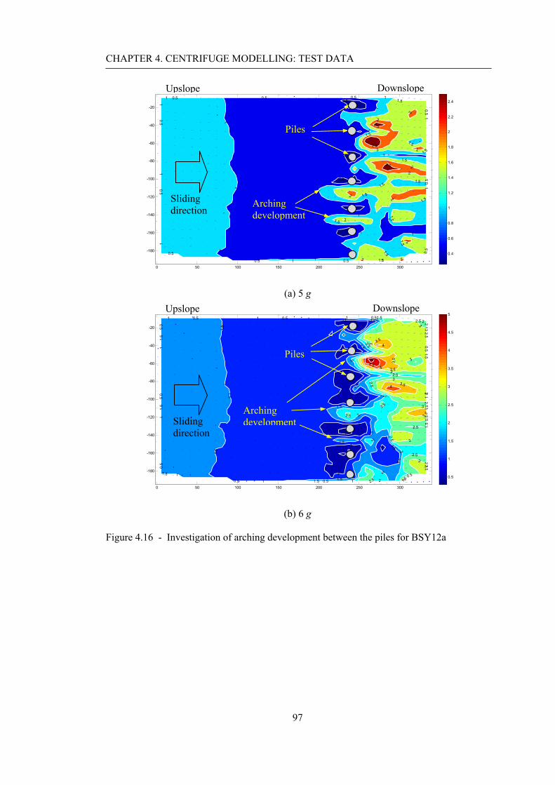
CHAPTER 4. CENTRIFUGE MODELLING: TEST DATA
97
0.5 0.5 0.5
0.5
0.5
0.5
0.50.5
0.5
0.50.5
1
1
1
1
1
11
1
1
1
1
1
11 1
1
1
1
1
1
1
1
1.5
1.5
1.5
1.5
1.51.5
1.5
1.5
2
2
1.5
1.522
1.5
1.5
2
1.5
0.5
0.5
0.5
0.5
2.5
0.5
1.5
2.5
2
2
2.5
2
2
22
2
0 50 100 150 200 250 300
-180
-160
-140
-120
-100
-80
-60
-40
-20
0.4
0.6
0.8
1
1.2
1.4
1.6
1.8
2
2.2
2.4
(a) 5 g
0.5 0.5 0.5
0.5
0.5
0.50.50.5
0.5
0.50.5
1 1 1
1
1
1
11
1
1
1
1.5
1 .5
1.51.5 1.5
1.5
1.5
1.5
1.5
1.51.5
1.5
1.5
1.5
1.5
1.5
1.5
22
2
2
2
2
2
2 2
2.52.5
2.5
2.5
2.5
2.5
2.5
3
33
3
11 3
3
1
1
1
1
1.5
1.5
2.5
2.5
3.5
3.5
33
2
2
3.5
1
4
3
1
3
3.5
2.5
3
3.5
4.5
1.5
0.5
4
2
1
5
2.5
2.5
2.5
1
3
4
2
0 50 100 150 200 250 300
-180
-160
-140
-120
-100
-80
-60
-40
-20
0.5
1
1.5
2
2.5
3
3.5
4
4.5
5
(b) 6 g
Figure 4.16 - Investigation of arching development between the piles for BSY12a
Piles
Upslope Downslope
Arching development
Arching development
Piles
Downslope Upslope
Sliding direction
Sliding direction

CHAPTER 4. CENTRIFUGE MODELLING: TEST DATA
98
0.5 0.5 0.5
0.5
0.5
0.50.50.5
0.50.5
0 .5
1 1 1
1
1
1111
1
1
1.5 1.5 1.5
1.5
1.5
1.5
1.51.51.5
1.5
1.5
1 .5
2 2 2
2
2
2
2
2
222
2
2
2.5
2.5
2.5 2.5
2.52.5
2.5
2.52.5
2.5
2.5
2.52.52.5
2.52.5
2 .5
33
3
3
3
3
3
3
3
3.5
3.5
3.5
3.5
3
3
3
33
4
4
4
3
3
3 3
3.5
3.5
3.5
4.5
4.5
4.5
3.5
3.5
3.53.5
4
4
4
2
2 2
44
4
1.5
1.5
2.5
2.5
3
3
5
5
2
2
4.5
4.5
3.5
3
1.5
4
4.5
1
31
3
3
1
5
50 100 150 200 250
-180
-160
-140
-120
-100
-80
-60
-40
-20
0.5
1
1.5
2
2.5
3
3.5
4
4.5
5
(a) 5 g
1 1 1
1
1
111
1
1
1
2 2 2
2
2
222
2
2
2
3 3 3
33
3
3
333
33
44
4
44
4
4
4
4
4
4
5
5
5
5
4
4
4
4
4
6
6
6
6
5
5
5
5 5
7
7
7
7
6
66
88
8
4
4
4
55
5 5
7
7
7
9
9
9
3
3 3
55
8
8
3 3
6
6
6
62
2
6
62
7
7
7
4
8
4
6
10
10
7
8
11
8
9
99
9
1
7
7
11
10
12
3
4
5
3
2
7
50 100 150 200 250
-180
-160
-140
-120
-100
-80
-60
-40
-20
1
2
3
4
5
6
7
8
9
10
11
12
(b) 6 g
Figure 4.17 - Flow action between the piles for BSY15d ((l/h) = 2.5, (s/d) = 8.9)
Pile
Sliding direction
Flow development
Piles
Sliding direction
Flow development
Upslope Downslope
Upslope Downslope

CHAPTER 4. CENTRIFUGE MODELLING: TEST DATA
99
4.2.4 Pile head displacements
Pile head displacement has been deduced using PIV analysis of a series of images of the
slope face. Figure 4.18 shows that the pile head displacement (δp, results normalised by pile
diameter) increases with an increase of gravity level (N) and (s/d) for a given (l/h), and with
(l/h) for a given (s/d). These trends all seem reasonable.
‘Normalisation’ of this data in this respect is considered in Figure 4.19, by dividing by the
product of all three variables above. It can be seen that the normalised displacements for all
tests generally tend toward consistency regardless of N, (s/d) and (l/h), although the value
tends to be slightly higher at low g-level in some tests. At higher g-level the results tend
towards an approximately unique value.
In fact the series of ‘normalising’ parameters reflect the total load on a single pile, which
tends to increase in proportion to N, (s/d) and (l/h) – this idea is pursued further in the
theoretical framework which is developed in Chapter 5. This indicates that the piles show
broadly consistent active response to loading throughout the tests, and have sufficient active
capacity in the underlying stable soil (significant active failure at any stage would
presumably have been indicated by increase of the ‘normalised’ secant displacement).

CHAPTER 4. CENTRIFUGE MODELLING: TEST DATA
100
0
0.2
0.4
0.6
0.8
1
1.2
0 10 20 30 40 50
δ p/ d
g-level (N)
2.53.64.55.9
(l/h) = 4.0(s/d) =
0
0.2
0.4
0.6
0.8
1
0 10 20 30 40 50
δ p/ d
g-level (N)
2.53.64.55.9
(l/h) = 3.0(s/d) =
0
0.2
0.4
0.6
0.8
1
0 10 20 30 40 50
δ p/ d
g-level (N)
2.53.64.55.98.9
(l/h) = 2.5(s/d) =
0
0.2
0.4
0.6
0.8
1
0 10 20 30 40 50
δ p/ d
g-level (N)
2.53.64.55.98.9
(l/h) = 2.0(s/d) =
0
0.2
0.4
0.6
0.8
1
0 10 20 30 40 50
δ p/ d
g-level (N)
2.53.64.55.98.9
(s/d) = (l/h) = 1.5
Figure 4.18 - Pile head displacements with g-level for all tests

CHAPTER 4. CENTRIFUGE MODELLING: TEST DATA
101
0
0.005
0.01
0.015
0.02
0.025
0 10 20 30 40 50
Nor
mal
ised
pile
dis
plac
emen
t, m
mδ p
/ {N
(s /d
) (l /
h)}
g-level (N)
12a 12b 14a 12c14b 11a 15f 14c12d 14d 13d 13b13c 13a 15e 15b13f 13e 14g 15a15d 11c 15c
Figure 4.19 - ‘Normalisation’ of pile displacement with g-level for all tests

CHAPTER 4. CENTRIFUGE MODELLING: TEST DATA
102
4.2.5 Relative pile-soil displacement
‘Relative’ pile-soil displacement (δr) is often used in the analysis of passive behaviour.
Figure 4.20 shows the general concept of δr that is employed frequently in numerical analysis.
Here the difference between the upslope soil movement observed at the ground surface (δu)
and the pile head movement (δp) is taken as a broad indicator of relative pile-soil
displacement.
Figure 4.21 shows results of relative pile-soil displacement for all tests – δr tends to increase
as both (s/d) and (l/h) increase. Note that the upslope soil movements were estimated by
averaging the available displacement vectors (upslope of the piles) in a test due to significant
loss of texture on the slope (also previously stated in Section 4.2.2). This trend seems to
logically indicate that:
1. Passive restraint of the stabilising piles to sliding of the slope becomes less effective
at wider (s/d) for given (l/h)
2. Large (l/h) generates greater passive loading for a given (s/d).
Figure 4.20 - General definition of relative pile-soil displacement in numerical analysis
Direction of sliding
δp
δu
δr
where, δr ( = δu - δp ) = Relative pile-soil displacement
Initial position of soil along pile row
Initial position of the pile
Deformed soil position
Deformed pile position, δp
Equivalent deformed soil position, δu

CHAPTER 4. CENTRIFUGE MODELLING: TEST DATA
103
0
1
2
3
4
5
6
0 10 20 30 40 50
δ r/ d
g-level (N)
2.53.64.55.9
(l/h) = 4.0(s/d) =
0
1
2
3
4
5
0 10 20 30 40 50
δ r/ d
g-level (N)
2.53.64.55.9
(l/h) = 3.0(s/d) =
0
1
2
3
4
5
0 10 20 30 40 50
δ r/ d
g-level (N)
2.53.64.55.98.9
(l/h) = 2.5(s/d) =
0
0.2
0.4
0.6
0.8
1
1.2
1.4
0 10 20 30 40 50
δ r/ d
g-level (N)
2.53.64.55.98.9
(l/h) = 2.0(s/d) =
0
0.2
0.4
0.6
0.8
1
1.2
1.4
0 10 20 30 40 50
δ r/ d
g-level (N)
2.53.64.55.98.9
(l/h) = 1.5(s/d) =
Figure 4.21 - Relative pile-soil displacement with g-level

CHAPTER 4. CENTRIFUGE MODELLING: TEST DATA
104
4.3 Pile moment data
Bending moment transducers (BMTs) were used to the measure the moment at discrete
points along the length of the pile (see Section 3.4.3). A curve-fitting technique was then
used to approximate continuous profiles of moment, shear force, and pressure from the
measured moment data.
4.3.1 Variation of moment with time
The continuous variations of electrical signals from each strain gauge location were recorded
for the pile during a test. Figure 4.22 shows typical variations of moment (differential output
voltages multiplied by a calibration factor) with time for BMT 6 (located at the elevation of
the interface) slip. Gravity level was increased throughout the test and the increments used
are also labelled.
Both results (BSY12a and BSY15a) show similar behaviour – larger increments in gravity
level at the end of the test tend to give correspondingly larger increments in moment.
Generally, the immediate response to increasing g-level (and hence passive loading) is
usually sizable, although there is also generally a surprisingly large time-related response
(particularly at low g-levels) given that the soil is dry sand. Each g-level was normally held
constant for approximately 5 minutes, so that an asymptotic value was approached. The
origins of the time-related behaviour were not established with certainty, but it seems likely
that creep in the greased interface caused ongoing downslope movement of the soil with time.

CHAPTER 4. CENTRIFUGE MODELLING: TEST DATA
105
0
0.5
1
1.5
2
2.5
3
3.5
4
4.5
5
0 1000 2000 3000 4000 5000 6000 7000
Mom
ent (
Nm
)
Time (sec)
(a) BSY12a
0
0.5
1
1.5
2
2.5
3
3.5
0 1000 2000 3000 4000 5000
Mom
ent (
Nm
)
Time (sec)
(b) BSY15a
Figure 4.22 - Variation of bending moment for BMT 6 (at the interface elevation) with time
50g 5g 16g 30g 1g increments 2g 4g Start End
5g 16g 30g 50g End
Start
1g increments 2g 4g

CHAPTER 4. CENTRIFUGE MODELLING: TEST DATA
106
4.3.2 Moment, shear force, and pressure profiles with depth
The pile is embedded through the unstable soil (passive loading) and into the stable material
(active loading) beneath. There is continuity of bending moment and shear force in the pile
across the predefined failure interface (i.e. silicon-greased latex/aluminium interface).
However there is a discontinuity of lateral pressure at the slip, due to the discontinuity of soil
displacements (and corresponding change from passive to active loading).
A form of spline curve-fitting technique was therefore employed, with separate polynomials
used to fit the measured bending moment data in each layer. The use of this technique is
advantageous in reducing the order of polynomials required to achieve satisfactory results,
and allowing pressure discontinuity at the slip. The polynomials were constrained to give:
(1) continuity of moment and shear force in the pile at the slip
(2) zero moment and shear force at the pile head and tip, and
(3) zero lateral pressure at the pile head (where the overburden stress is zero and hence
the strength of a cohesionless soil tends to zero).
The method of least squares is often used to give a unique ‘best fit’ of a polynomial to data.
Partial derivatives are derived to minimise the error between the data and the polynomial fit,
and the resulting equations give a unique solution via solution of simultaneous equations (i.e.
inversion of a matrix).
A cost function is a popular alternative technique for optimisation of mathematical problems,
which generally requires considerably more computational effort, but avoids the necessity of
deriving an explicit set of equations by hand to be solved. The additional computational
effort for a problem such as this is not that onerous by today’s standards, and the approach
offers considerable flexibility and convenience. The resulting solution is not strictly unique,

CHAPTER 4. CENTRIFUGE MODELLING: TEST DATA
107
but provided it has been obtained ‘correctly’ any such analysis would give a similar
optimised result.
Here a ‘cost function’ was implemented as follows:
• Derive the value of the polynomial multipliers an (passive zone) using one of the
methods described below. These values would then remain fixed.
• Make an initial arbitrary assumption regarding the value of the polynomial
multipliers bn (active zone) (see Figure 4.23 below).
• Define the total error in fitting the bending moment data at discrete depths as the
sum of the square errors for all data points compared to the polynomial fit.
• Add to this terms for ‘error’ in continuity of moment and shear force at the interface,
with an increased ‘weighting’ compared to fitting the data. Conditions at the head
and toe of the pile are inherently incorporated as described below, and hence do not
need to be considered in the cost function.
• Use optimisation functions in Matlab to minimise the total error from fitting the data
and continuity at the interface by adjusting the values bn. The increased weighting
for continuity at the interface means that this is satisfied accurately whilst the data is
subject to a ‘least squares’ fit.
The precise result obtained will depend on the technique for optimisation and the number of
iterations, as well as the weighting factor given to continuity at the interface. However,
provided there is sufficient iteration and the weighting factor is sufficiently large without
allowing even very small errors at the interface to have undue influence on the solution, the
result should be reasonable. The Matlab code to do this was developed in house (Cox, 2006).
One problem in polynomial curve fitting is the selection of an appropriate order for the
polynomial. It can be argued that in principle the use of higher order of polynomials

CHAPTER 4. CENTRIFUGE MODELLING: TEST DATA
108
provides a more detailed profile, allowing greater freedom of curve fitting. However the
results are generally unsatisfactory since high order curves tend to ‘oscillate’ between the
data points and are highly sensitive to relatively small variations (or errors) in moment. In
fact, the lowest order polynomial which gives a reasonable fit to the data is often most
suitable.
Figure 4.23 - Bending moment, shear force, and lateral pressure acting on the pile
Figure 4.23 shows a schematic diagram for the curve-fitting technique used here. BMT1 to 5
are in the passive zone (section a) and BMT 7 to 10 are in the active zone (section b). BMT6
is at the interface. Two different vertical co-ordinates systems are used (za and zb), measured
from the head and toe of the pile respectively. This offers considerable convenience in
inherently satisfying the conditions that moment and shear force should be zero at these
points.
Unstable upper layer BMT 1
za
Predefined failure slip
Underlying stable material
BMT 6
BMT10
Sliding direction
zb
Section a
(Passive zone)
Section b
(Active zone)

CHAPTER 4. CENTRIFUGE MODELLING: TEST DATA
109
Table 4.1 summarises the polynomials P1 and P2 used in the passive zone (za), and P3 used in
the active zone (zb). In the passive zone either the P1 or P2 approach was used – not both
simultaneously. In fact the initial polynomials describe the pressure distribution, and are
integrated to give shear force and bending moment. However no constants of integration are
introduced since shear force and bending moment are zero for za and zb = 0, and these
constraints are inherently incorporated. The assumption of zero lateral pressure at the pile
head also implies that there is no a0 term in P1 and P2.
The P1 approach allows ‘direct derivation’ of the only polynomial multiplier a1 based only
on the value of bending moment at the interface (BMT 6). The P2 approach used a true
‘least squares’ approach by inversion of a 2×2 matrix to obtain a1 and a2 based on all
bending moment data above the interface. The values bn were then optimised using a cost
function as described above.
Table 4.1 Curve fitting functions used for deriving moment, shear force, pressure profiles
P1 approach (direct derivation from BMT 6) P2 approach (least squares matrix inversion)
1( )a ap z a z= 21 2( )a a ap z a z a z= +
2
10
( ) ( )2
aza
a a azS z p z dz a= =∫
2 3
1 20
( ) ( )2 3
aza a
a a az zS z p z dz a a= = +∫
3
10
( ) ( )6
aza
a a azM z S z dz a= =∫
3 4
1 20
( ) ( )6 12
aza a
a a az zM z S z dz a a= = +∫
P3 approach (cost function)
20 1 2( )b b bp z b b z b z= + +
2 3
0 1 20
( ) ( )2 3
bzb b
b b b bz zS z p z dz b z b b= = + +∫
2 3 4
0 1 20( ) ( )
2 6 12bz b b b
b b bz z zM z S z dz b b b= = + +∫

CHAPTER 4. CENTRIFUGE MODELLING: TEST DATA
110
Derived profiles of moment, shear force, and pressure from the P1 and P2 approaches are
illustrated in Figure 4.24 and Figure 4.25 for typical data at 10, 20, and 30 g, where the red
dashed line shows the P1 data fit and the blue solid line is the P2 data fit. Use of the P1 or P2
curve in the passive zone also affects the P3 curve in the active zone due to the condition of
continuity of shear force at the interface. The numerical values of the polynomial terms
which have been derived for the moment data fit are recorded on the plots. ‘AAE’ is the
Average Absolute Error in fitting the data, whilst ‘RMSE’ is the root mean square error.
Both are expressed as a percentage of the maximum moment in the pile. The values shown
refer to the P2 (rather than P1) data fit.
Figure 4.24 shows reasonable consistency between the P1 and P2 data fits in all derived
profiles for BSY12a. However, in Figure 4.25 the P1 data fit for BSY15a gives problems in
the passive zone when the moment data at mid-depth in the passive zone is low, and the
cubic moment curve does not allow sufficient curvature as the moment data increases rapidly
towards the bottom of the passive zone.
Problems with the P1 data fit for BSY15a persist below the interface since the shear force at
the interface has potentially been underestimated, and hence the shear force is initially
approximately constant immediately below the interface (compared to reduction with depth
for the P2 data fit). This implies approximately zero pressure immediately below the
interface for the P1 data fit, increasing rapidly with depth. This does not seem consistent
with the general mode of pile deformation and the assumption that the soil below the
interface undergoes little movement. The pressure profile in the active zone given by the P2
data fit (in the passive zone) seems more reasonable.
In the passive zone a triangular distribution of limiting stress might be anticipated,
corresponding to increase of nominal overburden stress with depth. The greater than linear

CHAPTER 4. CENTRIFUGE MODELLING: TEST DATA
111
increase with depth shown for the P2 data fit in Figure 4.25 seems unlikely - somewhat less
than linear increase indicating some reduction in mobilisation compared to the ultimate value
with depth would be more plausible.
In general, 11 tests with a large (l/h) and small (s/d) gave similar (satisfactory) curve-fitting
to BSY12a, but the others (12 tests) with small (l/h) and large (s/d) tended to give similar
problems to BSY15a. This corresponds to the postulated mechanism of ‘shallow failure
passing through the piles’ in Figure 4.15. It seems likely that the surface of the slope may
actually have become slightly lower at the location of the pile row in these tests. This could
explain the difficulty in obtaining a good fit to the bending moment data using the P1
approach, since the nominal position assumed for the soil surface was no longer completely
accurate. With large (l/h) and small (s/d) a ‘bulge’ of soil tended to form behind the row
(Figure 4.3(e)), and hence there was less tendency for the level of the soil surface to drop,
and the P1 curve fit gave better results.
In conclusion, the P1 approach is considered to be more ‘robust’ in the passive loading zone
and less sensitive to any error in position of the soil surface, or inaccuracy in small moment
measured at mid-depth in passive zone. Hence it will be used in preference to the P2
approach in the remainder of the thesis when considering passive loading.
From Figure 4.24 and Figure 4.25, it can be seen that the general trends of behaviour do not
change with g-level. Passive loading (positive pressure, Figure 4.1) increases with depth and
shows a maximum value at the slip – the rather unlikely shape of the P2 data fit in some
cases was discussed above. Below this loading is actively resisted (negative pressure) in the
stable ground with a point of pressure reversal near the toe of the pile in the active zone to
give moment equilibrium of the pile. The bending moment reaches a maximum in the active
zone where the shear force is zero.
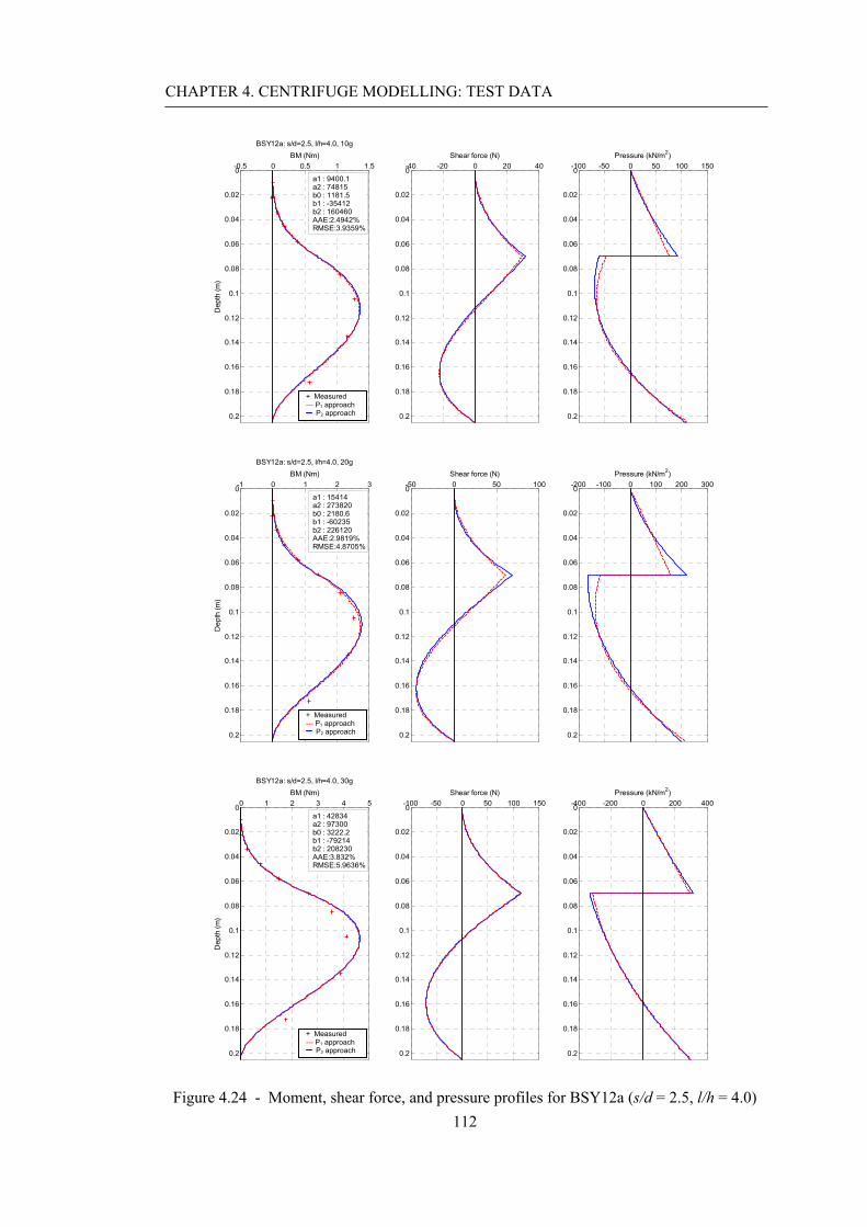
CHAPTER 4. CENTRIFUGE MODELLING: TEST DATA
112
-0.5 0 0.5 1 1.50
0.02
0.04
0.06
0.08
0.1
0.12
0.14
0.16
0.18
0.2
BM (Nm)
Dep
th (m
)
BSY12a: s/d=2.5, l/h=4.0, 10g
MeasuredCurve-fit
-40 -20 0 20 400
0.02
0.04
0.06
0.08
0.1
0.12
0.14
0.16
0.18
0.2
Shear force (N)-100 -50 0 50 100 1500
0.02
0.04
0.06
0.08
0.1
0.12
0.14
0.16
0.18
0.2
Pressure (kN/m2)
a1 : 9400.1a2 : 74815b0 : 1181.5b1 : -35412b2 : 160460AAE:2.4942%RMSE:3.9359%
-1 0 1 2 30
0.02
0.04
0.06
0.08
0.1
0.12
0.14
0.16
0.18
0.2
BM (Nm)
Dep
th (m
)
BSY12a: s/d=2.5, l/h=4.0, 20g
MeasuredCurve-fit
-50 0 50 1000
0.02
0.04
0.06
0.08
0.1
0.12
0.14
0.16
0.18
0.2
Shear force (N)-200 -100 0 100 200 3000
0.02
0.04
0.06
0.08
0.1
0.12
0.14
0.16
0.18
0.2
Pressure (kN/m2)
a1 : 15414a2 : 273820b0 : 2180.6b1 : -60235b2 : 226120AAE:2.9819%RMSE:4.8705%
0 1 2 3 4 50
0.02
0.04
0.06
0.08
0.1
0.12
0.14
0.16
0.18
0.2
BM (Nm)
Dep
th (m
)
BSY12a: s/d=2.5, l/h=4.0, 30g
MeasuredCurve-fit
-100 -50 0 50 100 1500
0.02
0.04
0.06
0.08
0.1
0.12
0.14
0.16
0.18
0.2
Shear force (N)-400 -200 0 200 4000
0.02
0.04
0.06
0.08
0.1
0.12
0.14
0.16
0.18
0.2
Pressure (kN/m2)
a1 : 42834a2 : 97300b0 : 3222.2b1 : -79214b2 : 208230AAE:3.832%RMSE:5.9636%
Figure 4.24 - Moment, shear force, and pressure profiles for BSY12a (s/d = 2.5, l/h = 4.0)
+ Measured --- P1 approach P2 approach
+ Measured --- P1 approach P2 approach
+ Measured --- P1 approach P2 approach

CHAPTER 4. CENTRIFUGE MODELLING: TEST DATA
113
-0.5 0 0.5 1 1.5 20
0.02
0.04
0.06
0.08
0.1
0.12
0.14
0.16
0.18
0.2
BM (Nm)
Dep
th (m
)
BSY15a: s/d=5.9, l/h=1.5, 10g
MeasuredCurve-fit
-40 -20 0 20 400
0.02
0.04
0.06
0.08
0.1
0.12
0.14
0.16
0.18
0.2
Shear force (N)-100 0 100 2000
0.02
0.04
0.06
0.08
0.1
0.12
0.14
0.16
0.18
0.2
Pressure (kN/m2)
a1 : 916.42a2 : 306270b0 : 1689.3b1 : -56322b2 : 302300AAE:2.5474%RMSE:4.0576%
-1 0 1 2 3 40
0.02
0.04
0.06
0.08
0.1
0.12
0.14
0.16
0.18
0.2
BM (Nm)
Dep
th (m
)
BSY15a: s/d=5.9, l/h=1.5, 20g
MeasuredCurve-fit
-100 -50 0 50 1000
0.02
0.04
0.06
0.08
0.1
0.12
0.14
0.16
0.18
0.2
Shear force (N)-200 0 200 4000
0.02
0.04
0.06
0.08
0.1
0.12
0.14
0.16
0.18
0.2
Pressure (kN/m2)
a1 : -6212.1a2 : 836500b0 : 3280.9b1 : -106480b2 : 544990AAE:2.8952%RMSE:4.7026%
-2 0 2 4 60
0.02
0.04
0.06
0.08
0.1
0.12
0.14
0.16
0.18
0.2
BM (Nm)
Dep
th (m
)
BSY15a: s/d=5.9, l/h=1.5, 30g
MeasuredCurve-fit
-100 -50 0 50 100 1500
0.02
0.04
0.06
0.08
0.1
0.12
0.14
0.16
0.18
0.2
Shear force (N)-400 -200 0 200 400 6000
0.02
0.04
0.06
0.08
0.1
0.12
0.14
0.16
0.18
0.2
Pressure (kN/m2)
a1 : -13507a2 : 1361800b0 : 5441.6b1 : -182440b2 : 981870AAE:2.8108%RMSE:4.8559%
Figure 4.25 - Moment, shear force, and pressure profiles for BSY15a (s/d = 5.9, l/h = 1.5)
+ Measured --- P1 approach P2 approach
+ Measured --- P1 approach P2 approach
+ Measured --- P1 approach P2 approach

CHAPTER 4. CENTRIFUGE MODELLING: TEST DATA
114
4.3.3 Derived and idealised pile displacements with depth
The pile displacement profile with depth can be derived by integrating the moment
polynomials (see Table 4.1) twice, as follows:
Passive zone (based on P2 approach)
4 5
1 2 10
1( ) ( )24 60
aza a
a a az zz M z dz a a A
EIθ
⎛ ⎞= = + +⎜ ⎟
⎝ ⎠∫
5 6
1 2 1 20
1( ) ( )120 360
aza a
a a a az zu z z dz a a A z A
EIθ
⎛ ⎞= = + + +⎜ ⎟
⎝ ⎠∫
Active zone (based on P3 approach)
3 4 5
0 1 2 10
1( ) ( )6 24 60
bzb b b
b b bz z zz M z dz b b b B
EIθ
⎛ ⎞= = + + +⎜ ⎟
⎝ ⎠∫
4 5 5
0 1 2 1 20
1( ) ( )24 120 360
bzb b b
b b b bz z zu z z dz b b b B z B
EIθ
⎛ ⎞= = + + + +⎜ ⎟
⎝ ⎠∫
The total four constants of integration (A1, A2, B1, and B2) are obtained by assuming:
(1) the pile deflection at the head is equal to the pile head displacement deduced from
image analysis in the test.
(2) continuity of gradient (rotation, θ) at the interface.
(3) continuity of pile displacement (u) at the interface.
(4) the point of pressure reversal in the active zone is assumed to correspond to zero
absolute pile deformation. In fact, this point is associated with zero differential
displacement between the pile and soil. However, this assumption will be
acceptable since lateral soil displacement is likely to be very small at this depth.

CHAPTER 4. CENTRIFUGE MODELLING: TEST DATA
115
This allows four independent equations to be written in terms of the four unknown constants
of integration. Hence a unique solution exists and can be derived (see Appendix A).
For convenience the profile of pile displacement with depth could be idealised assuming that
the pile is completely rigid. The idealised linear profile is assumed to be defined by the pile
displacement at the pile head, and zero absolute pile displacement at the point of pressure
reversal near the tip.
The resulting pile displacement (normalised by pile diameter) for BSY12a at 30 g (Figure
4.26) shows a typical results. The pile deflects downslope (the positive direction) – rotation
and flexure of the pile both contribute to this movement. The linear profile overestimates the
displacement above the point of pile rotation, which is around 40 % higher than the value
derived including the effect of flexure at the predefined slip.
0
2
4
6
8
10
12
14
16
18
20
-0.2-0.100.10.20.30.40.5
z / d
δp / d
Derived pile displacement profile
Linear pile displacement profile
The point of pressure reversal
Initial pile position
Predefined slip
Sliding direction
Figure 4.26 Derived and idealised pile displacement profiles with depth (BSY12a at 30g)

CHAPTER 4. CENTRIFUGE MODELLING: TEST DATA
116
4.4 Summary
Movements of the unstable soil mass in the cross sectional plane and on the face of the slope
during tests were successfully deduced from In-flight photography and digital image
processing (PIV analysis), including some important aspects of ground deformation.
General trends of displacement of the slope and the pile head can be described as follows:
• the ground and pile head displacements, and relative pile-soil displacement increase
with (s/d) for a given (l/h) and with (l/h) for a given (s/d)
• ‘upslope failure’ with a passive wedge above the pile row occurred for high (l/h) and
low (s/d)
• flow through the piles with large displacement occurred for high (l/h) and (s/d)
• shallow surface failure passing through piles occurred for low (l/h) and high (s/d)
• the slope was stable with small displacement at low (l/h) and (s/d)
Continuous distributions of moment, shear force, and pressure were derived from the
measured moment data using a curve-fitting technique (combined with the least squares
matrix inversion method or direct derivation in the passive zone and cost function in the
active zone). General behaviour of the piles can be summarised as follows:
• the bending moment increases with depth and reaches a maximum in the active zone
where the shear force is zero
• the pressure in the passive zone increases approximately linearly with depth,
showing a maximum at the slip
• below the slip the pressure is actively resisted in the stable material with a point of
pressure reversal in the active zone to give moment equilibrium of the pile
Interpretation of the centrifuge test data will be presented in Chapter 5

117
CHAPTER 5
CENTRIFUGE MODELLING:
INTERPRETATION AND COMPARISON
5.1 Introduction
This chapter presents a theoretical framework that is based on analysis of a semi-infinite
slope. The centrifuge test data are interpreted by comparison with the proposed framework.
Some of the previous work presented in Chapter 2 is then compared with the framework.
5.2 Theoretical framework for a piled slope
A theoretical framework (based on a conventional analysis of a semi-infinite slope under
‘plane strain’ conditions) is proposed to enhance generic understanding of slope stabilisation
using a row of piles. The framework primarily considers stabilisation of a potentially
unstable layer, focusing on evaluating the force required to stabilise the layer upslope of the
piles and the maximum stabilising force available from passive interaction.

CHAPTER 5. CENTRIFUGE MODELLING: INTERPRETATION AND COMPARISON
118
5.2.1 Problem definition
A uniform slope inclined at an angle β° to the horizontal is considered. A translational
failure slip has developed on a plane parallel to the surface of the slope and at a depth h m
below it (Figure 5.1). The l m long failing upslope soil block above the pile row (ABCD)
was considered to represent the effect of a failing mass of soil acting on the pile row. The
analogy with the centrifuge test approach (described in Chapter 4) is clear.
The end forces P1 and P2 due to the earth pressure on the interfaces AD and BC are assumed
to be equal and opposite (P1 does not include the effect of pressure on the piles, which will
be considered in due course). It is probable that the earth pressure will be close to active at
both these locations. The material downslope of the piles was unstable but active earth
pressure represents minimum support to the upslope material from the downslope material.
Figure 5.1 - Idealisation of a piled slope problem for semi-infinite slope
W
Tb
Nb
h
l
P1
Crest
Position of the pile row (AD)
Translational failure slip
P2
A
D
B
C β Ts (×2)
CHAPTER 5. CENTRIFUGE MODELLING: INTERPRETATION AND COMPARISON
119
The factor of safety (in terms of force equilibrium) is generally calculated by comparing
resisting forces with driving forces, and defined as
r
d
Resisting forces ( )FoS =Driving forces ( )
FF
(5.1)
Here resisting forces are the shear strength of the soil along the failure plane, and resistance
induced from any reinforcing members. An additional small component of resistance results
from side friction in the centrifuge tests. The driving force is the component of the gravity
load of the soil mass acting down the slope.
The weight of the upslope block of the failing soil (for a width b normal to the plane strain
section along the pile row) is given by
γlhbW = (5.2)
where,
l = length of upslope ‘block’
h = thickness of slip (from the surface to the slip)
b = width into page
The ‘disturbing’ component of this force will be taken as the component acting ‘down’ the
slope, giving
d sinF W β= (5.3)
Movement of the failing upslope block in the centrifuge model is resisted by friction
mobilised on the ‘front’ and ‘back’ sides Ts (assumed to act parallel to base), as well as
friction on the base, Tb. The general magnitude of these effects will be considered before
proceeding to consider resistance from the pile row.

CHAPTER 5. CENTRIFUGE MODELLING: INTERPRETATION AND COMPARISON
120
2s s s s s s s
1 12 2
hT N K h l K Wb
μ μ γ μ= = = (5.4)
and
b b b b cosT N Wμ μ β= = (5.5)
(assuming Nb = Wcosβ by resolving perpendicular to the base)
where,
Ts, Ns = Shear and Normal forces on each side
Tb, Nb = Shear and Normal forces on base
μs, μb = Coefficients of friction on sides and base (= tan δ)
Ks = Coefficient of earth pressure on sides
The total resistance from friction on the sides and base opposing the driving force Fd is
Fμ = (2Ts + Tb) (there are 2 sides). Thus expressing this relative to the nominal value of Fd
μ s bs s b
d
2 1 cossin sin
F T T hKF W b
μ μ β αβ β
+ ⎛ ⎞= = + =⎜ ⎟⎝ ⎠
(5.6)
where α is the total frictional resistance expressed relative to the driving force.
For a truly plane strain situation μs is effectively zero, so that
μ b
d tanFF
μβ
= (5.7)
corresponding to the normal equation for an infinite slope in purely frictional soil.
Coefficients of friction on the sides and base, μs and μb, have been determined by shear box
tests in the lab, e.g. μs = μb ≈ 0.03 (for 'intφ ≈ 2° in Section 3.6.1) but this is likely to vary in
the test models to some extent. Since the soil is assumed not to deform in the plane strain
direction, Ks may be estimated using the earth pressure coefficient at rest ( '0 1 sinK φ= − ).
Considering an upper bound on the effect of friction, taking μs = μb ≈ 0.1 (corresponding to

CHAPTER 5. CENTRIFUGE MODELLING: INTERPRETATION AND COMPARISON
121
'intφ ≈ 6°), Ks = 0.47 (for 'φ = 32°), and h/b = 0.36 (for h = 0.07 m and b = 0.196 m), α ≈ 0.1,
resulting mainly from the friction on the base.
Now consider the effect of a stabilising (shear) force S acting on the unstable soil mass,
compared to the disturbing force. The forces are pragmatically assumed to act upward along
the slip and hence can be directly compared (assuming that S maintains equilibrium by
resisting the driving force after subtracting the effect of friction).
d μ d (1 )S F F F AWα= − = − = (5.8)
where
(1 )sinA α β= − (5.9)
Note that the total horizontal stabilising force required for equilibrium is sometimes
considered (e.g. two part wedge method in HA68/94; Department of Transport, 1994) so that
tanβ replaces sinβ. However, for typical values of β for soil slopes there is little practical
difference between these results.
5.2.2 Stabilising (shear) force
A stabilising (shear) force that each pile can provide to resist sliding of the slip is now taken
into account. A triangular passive load distribution is assumed and hence the stabilising
interaction force on a pile is given by
2p mob
12
S B h dγ= (5.10)
where,
Sp = total stabilising interaction force on a pile (normal to the pile),
equivalent to the shear force at the sliding interface

CHAPTER 5. CENTRIFUGE MODELLING: INTERPRETATION AND COMPARISON
122
Bmob = lateral interaction stress on pile / nominal vertical stress, assumed
constant with depth
This normalised lateral interaction stress (Bmob) may be proposed to tend to a value such as
Kp2 (as proposed in Equation (2.3)) as the interaction reaches its ultimate state.
For stability of the slope the required stabilising force (Equation 5.8) and the interaction
forces for n piles across the width b can be equated:
2p mob
12
S nS B h nd AW Albhγ γ= = = = (5.11)
Rearranging the above equation gives
mob 2 l bB Ah nd
⎛ ⎞⎛ ⎞= ⎜ ⎟⎜ ⎟⎝ ⎠⎝ ⎠
Substituting for pile spacing s = (b/n):
mob 2 l sB Ah d
⎛ ⎞⎛ ⎞= ⎜ ⎟⎜ ⎟⎝ ⎠⎝ ⎠
(5.12)
This relationship shows how the lateral interaction stress on the piles (expressed as Bmob)
required for stabilising the slope increases in proportion to:
1. A which incorporates the slope angle (β) and any reduction in ‘driving’ force due to
friction in the model
2. the length of the upslope soil block above the pile row relative to the thickness of
the sliding block (l/h)
3. the centre-to-centre spacing relative to the pile diameter (s/d)

CHAPTER 5. CENTRIFUGE MODELLING: INTERPRETATION AND COMPARISON
123
5.2.3 Pile row interaction
The general behaviour of a pile row due to passive interaction can potentially be specified by
considering the following concepts of limiting interaction capacity for a pile in a row
(Durrani, 2006):
• The pile behaves as an ‘isolated pile’, with the ultimate lateral resistance predicted
by (Fleming et al., 1994, Figure 5.2(a))
2 'p,ult p v0p K σ= (5.13a)
• The pile behaves as if it is part of a ‘continuous wall’ (i.e. arching is effective,
Figure 5.2(b)), with passive and active earth pressure in front of and behind it
respectively. In some cases there may be complete loss of support rather than active
earth pressure. However numerically (Kp – Ka) and (Kp – 0) are quite similar. If the
piles are not required for stability the upslope and downslope earth pressures may be
equal. Hence the equivalent pressure on the pile itself is given by
'p,ult p a v0( ) sp K K
dσ ⎛ ⎞= − ⎜ ⎟
⎝ ⎠ (5.13b)
where,
pp,ult = ultimate equivalent pressure on the pile (defined as the load per unit
length along the pile divided by the diameter)
Kp, Ka = the passive and active earth pressure coefficients respectively
a1 sin '1 sin '
K φφ
−=
+
pa
1 1 sin '1 sin '
KK
φφ
+= =
−
σ'v0 = the nominal vertical effective stress in the soil for a given depth

CHAPTER 5. CENTRIFUGE MODELLING: INTERPRETATION AND COMPARISON
124
s = centre-to-centre pile spacing
d = pile diameter
The ultimate equivalent pressure on the pile can be normalised by the initial vertical stress in
the soil since this term appears in both equations.
Figure 5.2 - Concepts of limiting interaction capacity for a pile in a row
For sloping ground Kp and Ka can be sometimes expressed as a function of slope angle (β°)
and internal friction angle of soil ( 'φ ). In Equation (5.13a) the term Kp is associated with
inherent limiting strength for a Mohr circle of stress, and modification of the value due
sloping ground would not be consistent with the basis of the formula. In Equation (5.13b)
the value of pp,ult derived using unmodified earth pressure coefficients is ‘conservative’,
whereas using values modified for a slope could potentially be ‘non-conservative’ (giving a
higher value of ultimate interaction). It is therefore considered pragmatic to use the
‘standard’ (unmodified) values of Kp and Ka.
The relationship between two equations (Equations (5.13a) and (5.13b)) proposes a rational
approach for predicting a critical spacing, (s/d)crit where the two equations intersect, and is
given by (Durrani, 2006)
pK
aK
(b) Continuous wall
2pK
(a) Isolated pile

CHAPTER 5. CENTRIFUGE MODELLING: INTERPRETATION AND COMPARISON
125
2p
crit p a
Ksd K K
⎛ ⎞ =⎜ ⎟ −⎝ ⎠ (5.14)
This expression represents a ‘general’ limit of the spacing ratio (s/d) at which arching is
effective. At wider spacings the piles are supposed to behave approximately as an isolated
pile (at least in terms of ultimate capacity). For instance for 'φ = 32°, (s/d) = 3.6 - this value
shows good general correspondence with generally accepted limits on the critical spacing for
arching to occur when using discrete pile rows for slope stabilisation.
5.3 Interpretation and comparison
Throughout this section, the centrifuge test results will be interpreted and compared with the
theoretical framework proposed in Section 5.2.
5.3.1 Interpretation of test data
Interpretation of the centrifuge test data will focus on the effect of the stabilising force at the
pre-defined slip interface (see Section 4.3.2), in order to determine the two variables A and
Bmob:
1. The total stabilising interaction force on an instrumented pile is derived from the
bending moment measured at the pre-defined slip interface (Mint), assuming that the
lateral force acts at a distance of (h/3) above the interface (corresponding to a
triangular distribution of load on the pile over the height h of unstable material,
Figure 5.1). Thus
intp, int ( / 3)
MSh
= (N) (5.15)
CHAPTER 5. CENTRIFUGE MODELLING: INTERPRETATION AND COMPARISON
126
2. The weight of the upslope unstable soil block above the pile row (W) is calculated by
considering the volume, density, and centrifugal acceleration (Ng),
W lbh lbh gNγ ρ= = (N) (5.16)
For the purposes of this calculation any small change (reduction) in l due to
movement of the upslope block is neglected.
3. The value A is calculated using the following relationship where n is the number of
the piles in the test,
p,intnSSAW W
= = (5.17)
According to the model of behaviour proposed this value is theoretically given by
Equation (5.9) as (1 - α) sinβ and thus correspondence with the model can be tested.
4. The value of Bmob is determined directly by substituting the derived stabilising force
into Equation (5.10)
p,int p,intmob 2 2
2 2S SB
h d gNh dγ ρ= = (5.18)
Again this theoretical value is given by Equation (5.11) as 2A(l/h)(s/d) and thus
correspondence with the model can be examined.

CHAPTER 5. CENTRIFUGE MODELLING: INTERPRETATION AND COMPARISON
127
5.3.2 Variation of A and B with g-level in each test
Figure 5.3 and Figure 5.4 show variation of the values of A and Bmob derived from the test
data (Mint and hence Sp,int) as described above, and plotted against increasing g-level in all the
tests. Each subplot shows a particular value of (l/h), whilst the various lines show various
(s/d).
Generally speaking, A is approximately constant with g-level for each test (Figure 5.3). This
is reasonable since the effect of g-level is accounted for by the γ term in Equation (5.16).
The maximum value is approximately 0.3 to 0.4, which is broadly consistent with the
theoretical value (according to Equation (5.9) Amax ≈ 0.45 for μb = μs ≈ 0.1 used in Section
5.2). Tests with high (s/d) can show lower values due to the effect of Bmax – further
discussion will be given in Section 5.3.4.
Again, it can be seen that Bmob is approximately constant with g-level for each test
(Figure 5.4) since this effect is again accounted for by the γ term in Equation (5.18). The
maximum value observed in any of the tests is Bmax ≈ Kp2. This normalised value is constant
with depth for the approximately triangular distribution of stress over the depth of passive
loading (Section 4.3.2), but this observation is probably associated with the use of a pre-
defined low friction failure interface. In a more general situation the passive pressure is
likely to reduce more gradually to zero at some depth. Generally speaking for a given value
of (l/h) Bmob tends to increase with (s/d), and for a given value of (s/d) Bmob tends to increase
with (l/h) – this is consistent with Equation (5.12).

CHAPTER 5. CENTRIFUGE MODELLING: INTERPRETATION AND COMPARISON
128
0
0.1
0.2
0.3
0.4
0.5
0 10 20 30 40 50
A
g-level (N)
2.5 3.64.5 5.9
(l/h) = 4.0
(s/d) =
0
0.1
0.2
0.3
0.4
0.5
0 10 20 30 40 50
A
g-level (N)
2.5 3.64.5 5.9
(l/h) = 3.0
(s/d) =
0
0.1
0.2
0.3
0.4
0.5
0 10 20 30 40 50
A
g-level (N)
2.5 3.64.5 5.98.9
(l/h) = 2.5
(s/d) =
0
0.1
0.2
0.3
0.4
0.5
0 10 20 30 40 50
A
g-level (N)
2.5 3.64.5 5.98.9
(l/h) = 2.0
(s/d) =
0
0.1
0.2
0.3
0.4
0.5
0 10 20 30 40 50
A
g-level (N)
2.5 3.64.5 5.98.9
(l/h) = 1.5
(s/d) =
Figure 5.3 - Variation of A with g-level for all tests

CHAPTER 5. CENTRIFUGE MODELLING: INTERPRETATION AND COMPARISON
129
0
2
4
6
8
10
12
14
16
0 10 20 30 40 50
B mob
g-level (N)
2.5 3.64.5 5.9
(l/h) = 4.0
(s/d) =
0
2
4
6
8
10
12
0 10 20 30 40 50
B mob
g-level (N)
2.5 3.64.5 5.9
(l/h) = 3.0
(s/d) =
0
2
4
6
8
10
12
0 10 20 30 40 50
B mob
g-level (N)
2.5 3.64.5 5.98.9
(l/h) = 2.5
(s/d) =
0
2
4
6
8
10
12
0 10 20 30 40 50
B mob
g-level (N)
2.5 3.64.5 5.98.9
(l/h) = 2.0
(s/d) =
0
2
4
6
8
0 10 20 30 40 50
B mob
g-level (N)
2.5 3.64.5 5.98.9
(l/h) = 1.5
(s/d) =
Figure 5.4 - Variation of Bmob with g-level for all tests

CHAPTER 5. CENTRIFUGE MODELLING: INTERPRETATION AND COMPARISON
130
5.3.3 Variation of A and Bmob with (s/d)
The values of A and Bmob deduced from all the tests are compared with the proposed
theoretical model in Figure 5.5 and Figure 5.6 respectively. The plots show variation with
(s/d) for a given (l/h).
As previously noted the value of A throughout a test showed relatively little variation
(Figure 5.3). The ‘representative’ value of A shown in Figure 5.5 as a data point was taken
over the range from 6 g to 10 g where the values were less affected by upslope displacement
and passive failure – this was also often the maximum value observed in the test. The
approximate upper limit (AUL) and lower limit (ALL) of Amax for the data are taken as 0.4
and 0.3 respectively, with the mean value of Amax also plotted at 0.35. As noted previously
this value shows reasonable correspondence with the theoretical estimate (Equation (5.9)).
In fact, the model of behaviour developed earlier in this Chapter indicates that the ‘true’
theoretical maximum value of A may not be observed in the pile loading. Re-arranging
Equation (5.12) in terms of Bmob (although it is more fundamentally related to Sp,int in terms
of it’s derivation from the data):
mobmax2( / )( / )
BA As d l h
= ≤ (5.19a)
For low (s/d) or (l/h) Amax will be observed, with a corresponding value of Bmob loading the
piles. In other words the action of the unstable soil mass dictates the load on the piles.
However, if the limiting interaction pressure (Bmax) is mobilised this limits the value of A
which is ‘observed’ in the test
maxmax2( / )( / )
BA As d l h
= < (5.19b)

CHAPTER 5. CENTRIFUGE MODELLING: INTERPRETATION AND COMPARISON
131
This also implies that the interaction has reached its ultimate ‘failure’ state. Taking Bmax as
2pK = 10.6 this curve is plotted at high (s/d) in Figure 5.5. The interaction of this line with
Amax is given by
max
int max
1 12 ( / )
Bsd A l h
⎛ ⎞ =⎜ ⎟⎝ ⎠
(5.20)
and hence tends to increase as (l/h) reduces. Based on the model, for a given (l/h), as (s/d)
increases initially Bmob increases (see Equation 5.21 below), since there are less piles to carry
the same load. Eventually Bmax is reached, with subsequent increase in (s/d) leading to
reduction in A as deduced from the limiting interaction.
The data points representing the tests in Figure 5.5 generally represent (s/d) less than the
intersection value (particularly for low (l/h)), and hence Amax is observed in the test.
However, there is some evidence of tendency for A to reduce as the intersection point is
approached and exceeded.
The ‘representative’ value of Bmob was obtained from Figure 5.4 in the same way as
described above for A. The results are plotted as data points in Figure 5.6. The
corresponding form of the equation for the model of behaviour is:
mob max max2 s lB A Bd h
⎛ ⎞⎛ ⎞= ≤⎜ ⎟⎜ ⎟⎝ ⎠⎝ ⎠
(5.21)
As (s/d) or (l/h) increase Bmob tends to increase until the limiting value of interaction is
reached. The value of (s/d) where the limit Bmax is reached is the same as above.

CHAPTER 5. CENTRIFUGE MODELLING: INTERPRETATION AND COMPARISON
132
Again the data generally represent (s/d) less than the intersection value (particularly for low
(l/h)). In fact the data have been derived from the same value of Sp,int and thus show the
same relationship with the proposed model of behaviour as in Figure 5.5.
Plotting the data in this way it is evident that for BSY15b ((s/d) = 5.9 and (l/h) = 4.0) Bmob
somewhat exceeds the proposed value of Bmax, whilst for BSY15c ((s/d) = 8.9 and (l/h) = 1.5)
it is somewhat less. Nonetheless the centrifuge test data derived generally shows good
agreement with the theoretical lines.
0
0.1
0.2
0.3
0.4
0.5
0 1 2 3 4 5 6 7 8 9 10
A
s / d
Centrifuge test data
AUL
ALLAmax
Equation (5.19b)
AVG
(l/h) = 4.0Equation(5.19a)
Equation (5.20)
(a)
0
0.1
0.2
0.3
0.4
0.5
0 1 2 3 4 5 6 7 8 9 10
A
s / d
AUL
ALLAmax AVG
(l/h) = 3.0
(b)

CHAPTER 5. CENTRIFUGE MODELLING: INTERPRETATION AND COMPARISON
133
0
0.1
0.2
0.3
0.4
0.5
0 1 2 3 4 5 6 7 8 9 10
A
s / d
AUL
ALLAmax AVG
(l/h) = 2.5
(c)
0
0.1
0.2
0.3
0.4
0.5
0 1 2 3 4 5 6 7 8 9 10 11 12
A
s / d
AUL
ALLAmax
AVG
(l/h) = 2.0
(d)
0
0.1
0.2
0.3
0.4
0.5
0 1 2 3 4 5 6 7 8 9 10 11 12 13 14
A
s / d
AUL
ALLAmaxAVG
(l/h) = 1.5
(e)
Figure 5.5 - Variation of A with various (s/d) for a given (l/h)

CHAPTER 5. CENTRIFUGE MODELLING: INTERPRETATION AND COMPARISON
134
0
2
4
6
8
10
12
14
16
0 1 2 3 4 5 6 7 8 9 10
B mob
s / d
Centrifuge test data
AUL ALL
Bmax = Kp2
Equation (5.21)
AVG(l/h) = 4.0
Equation (5.20)
(a)
0
2
4
6
8
10
12
14
16
0 1 2 3 4 5 6 7 8 9 10
B mob
s / d
AUL ALLBmax = Kp
2
AVG(l/h) = 3.0
(b)
02468
10121416
0 1 2 3 4 5 6 7 8 9 10
B mob
s / d
AUL ALL
Bmax = Kp2
AVG(l/h) = 2.5
(c)

CHAPTER 5. CENTRIFUGE MODELLING: INTERPRETATION AND COMPARISON
135
02468
10121416
0 1 2 3 4 5 6 7 8 9 10 11 12
B mob
s / d
AULALL
Bmax = Kp2
AVG(l/h) = 2.0
(d)
02468
10121416
0 1 2 3 4 5 6 7 8 9 10 11 12 13 14
B mob
s / d
AUL ALL
Bmax = Kp2
AVG(l/h) = 1.5
(e)
Figure 5.6 - Variation of Bmob with (s/d) for a given (l/h)
CHAPTER 5. CENTRIFUGE MODELLING: INTERPRETATION AND COMPARISON
136
5.3.4 Relationship between pile row interaction, (s/d) and (l/h)
Figure 5.7 summarises the previous observations regarding variation of A and Bmob as (s/d)
changes for given (l/h).
Re-arranging Equation (5.21) above:
mob
max
1 12 ( / )
Blh A s d
⎛ ⎞ =⎜ ⎟⎝ ⎠
(5.22)
Thus expressing the value of (l/h) theoretically required to mobilise a given value of B in
terms of pile-soil interaction for a given value of (s/d). It is assumed that Bmob ≤ Bmax, and
thus A = Amax = 0.35.
Figure 5.8 shows this relationship for Bmob = Kp2 and Bmob = Kp. As above, the former value
is proposed as the limiting interaction stress (for an ‘isolated’ pile). The latter value is a
‘factored’ value of interaction which represents reduced mobilisation of interaction (Durrani,
2006). In fact the model of behaviour proposed by Durrani incorporates a minimum value of
(s/d) below which ‘isolated’ behaviour is no longer applicable, and the limiting resistance
offered by the pile row shows no further increase (the pile row acts as a ‘continuous wall’).
This limit is given by Equation (5.14), and is shown on Figure 5.8. The value of (l/h) for
each value of Bmob shows no further increase as (s/d) reduces beyond this point.
For the purpose of simplification three labels are defined on the plot (Figure 5.8):
A. small interaction pressure required for stability
B. increasing interaction pressure required for stability
C. proposed ultimate interaction pressure exceeded

CHAPTER 5. CENTRIFUGE MODELLING: INTERPRETATION AND COMPARISON
137
Figure 5.7 - Concept of the pile row interaction in terms of A and Bmob
0
1
2
3
4
5
6
0 1 2 3 4 5 6 7 8 9 10 11 12
l / h
s/d
Factored limit: Bmob = Kp
Unfactored limit:Bmax = Kp
2
Equation (5.14): (s/d)crit = Kp
2/(Kp - Ka)
A
B
C
Figure 5.8 - Concept of the pile row interaction in terms of (l/h) and (s/d)
Bmob Bmax = Kp2
(s/d)
AA = Amax B = Bmob
(s/d)
(s/d)int
A = Amax B = Bmax
A = Amob B = Bmax = Kp
2

CHAPTER 5. CENTRIFUGE MODELLING: INTERPRETATION AND COMPARISON
138
Figure 5.9 attempts to correlate the amount of interaction which is ‘mobilised’ in a test
(based on the proposed model of behaviour) with the normalised relative displacement
measured at 50 g on the plot of (l/h) and (s/d). Different data symbols have been used to
show different amounts of displacement, with corresponding line colours showing lines of
approximately equal displacement. Generally speaking deformation tends to increase with
mobilisation as expected. This shows good agreement with the deformation characteristics
presented in Section 4.2.3 (see Chapter 4).
0
1
2
3
4
5
6
0 1 2 3 4 5 6 7 8 9 10 11 12
l / h
s/d
3d - 5d 2d - 3d1d - 2d 0.5d -1d0.25d - 0.5d 0 - 0.25d
'Upslope' failure (passive wedge)
Normalised displacement δr
Large deformation(flow through piles)
Small deformation
Shallow failure (passing through piles)
0.25d0.5d
1d2d
3d5d
Figure 5.9 - Comparison of test results with the theoretical lines for relative displacement
CHAPTER 5. CENTRIFUGE MODELLING: INTERPRETATION AND COMPARISON
139
Figure 5.10 plots the normalised relative displacement at 50 g in all tests against the
(approximately constant) value of Bmob in the test. Separate data series show each value of
(s/d) used in the tests. Moving along a data series from left to right shows increase of (l/h) in
various tests, and hence increasing load on the pile row. The movement cannot be
interpreted directly as equivalent prototype values since it accumulated at a variety of g-
levels. However, the results from the various tests can be compared.
With the exception of one value at very large relative displacement as noted above Bmob tends
to a maximum value of approximately 10, approximately equal to Kp2. It could be argued
that a larger value would have been observed at higher δr. This would have required a test
with (l/h) > 4. However, the test package would not allow this, and in any case there would
have been very significant tendency for failure upslope of the piles, thus limiting interaction
with the piles.
For a given magnitude of Bmob less than the limiting value it can be seen that the value of
(s/d) does not have significant impact on the corresponding magnitude of δr. This supports
another observation by Durrani (2006) that piles spaced wider than the critical value still
offer support to the upslope material – it is just that the equivalent value per metre along the
slope drops in proportion to (1/s) for a given value of Bmob.

CHAPTER 5. CENTRIFUGE MODELLING: INTERPRETATION AND COMPARISON
140
0
2
4
6
8
10
12
14
16
0 1 2 3 4 5
B mob
δr / d
2.5 3.6 4.55.9 8.9
Kp2
(s/d) =
Figure 5.10 - Variation of Bmob with relative soil-pile displacement at 50 g showing results
from all tests
CHAPTER 5. CENTRIFUGE MODELLING: INTERPRETATION AND COMPARISON
141
5.4 Comparison with previous works
It is not possible to give direct comparison of the current work with all the references in
Chapter 2. However, it is possible to consider the interaction pressure on piles as it varies
with (s/d), and the design for a case study.
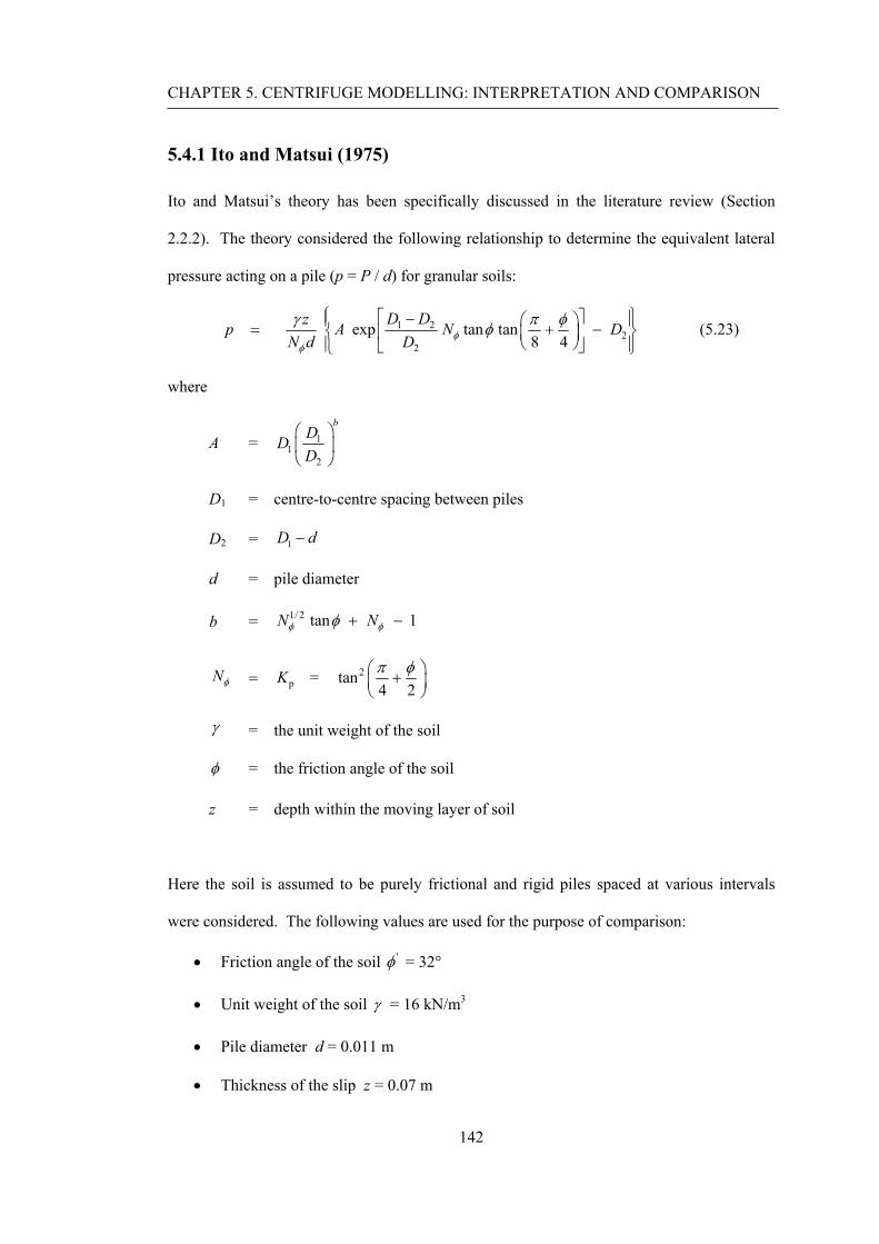
CHAPTER 5. CENTRIFUGE MODELLING: INTERPRETATION AND COMPARISON
142
5.4.1 Ito and Matsui (1975)
Ito and Matsui’s theory has been specifically discussed in the literature review (Section
2.2.2). The theory considered the following relationship to determine the equivalent lateral
pressure acting on a pile (p = P / d) for granular soils:
1 22
2exp tan tan
8 4D Dzp A N D
N d D φφ
γ π φφ⎧ ⎫⎡ ⎤−⎪ ⎪⎛ ⎞= + −⎨ ⎬⎢ ⎥⎜ ⎟
⎝ ⎠⎪ ⎪⎣ ⎦⎩ ⎭ (5.23)
where
A = 11
2
bDDD
⎛ ⎞⎜ ⎟⎝ ⎠
D1 = centre-to-centre spacing between piles
D2 = 1D d−
d = pile diameter
b = 1/ 2 tan 1N Nφ φφ + −
Nφ = pK = 2tan4 2π φ⎛ ⎞+⎜ ⎟
⎝ ⎠
γ = the unit weight of the soil
φ = the friction angle of the soil
z = depth within the moving layer of soil
Here the soil is assumed to be purely frictional and rigid piles spaced at various intervals
were considered. The following values are used for the purpose of comparison:
• Friction angle of the soil 'φ = 32°
• Unit weight of the soil γ = 16 kN/m3
• Pile diameter d = 0.011 m
• Thickness of the slip z = 0.07 m

CHAPTER 5. CENTRIFUGE MODELLING: INTERPRETATION AND COMPARISON
143
Figure 5.11 plots the ultimate pressure (pp,ult) on the pile normalised by the nominal
overburden stress (σ'v0 = γz) at any depth, which can be derived directly from Equation
(5.23). Expressing Equation (5.23) in this way all terms are non-dimensional (D1 and D2 are
normalised by d). Hence model-scale values can be used and are applicable to any g-level in
the centrifuge tests.
Normalising pp,ult in this way is equivalent to Bmob in the centrifuge tests (Equation (5.18)),
which was indeed found to be approximately constant in each test (Section 5.3.2). Hence
data corresponding to Figure 5.6 is plotted in Figure 5.11 for comparison. Equivalent limits
proposed by Durrani (2006) (Figure 2.5: ‘continuous wall’ and ‘isolated pile’) are also
shown.
Referring to Figure 5.11 some consistency between the centrifuge test data and Durrani’s
limits is evident. The ‘isolated pile’ limit is reached at wide spacing except when (l/h) = 1.5,
where presumably the upslope material was insufficient to generate full passive resistance
even at wide pile spacing. The widest spacing for (l/h) = 4 somewhat exceeds the isolated
pile limit. However, at lower spacing this data supports the ‘continuous wall’ limit proposed
by Durrani. For smaller (l/h) it would appear that the upslope material is again insufficient
to generate the full ‘continuous wall’ load.
However, from Figure 5.11 it can be seen that the Ito & Matsui method predicts the opposite
of the general trend observed from the centrifuge tests and Durrani’s method. The result
was found to tend toward the lower ‘factored limit’ proposed by Durrani as spacings get
wider. This is because the solution includes Nφ = Kp (the same as the factored limit for an
isolated pile proposed by Durrani). In conclusion, as noted by previous authors and
confirmed here, this method does not appear to give reasonable predictions of ultimate
resistance at small pile spacings (where the lateral force on the piles tends to infinity) and at

CHAPTER 5. CENTRIFUGE MODELLING: INTERPRETATION AND COMPARISON
144
wide spacings (where it tends to zero). At intermediate spacings (3 to 5d) the general trend
of behaviour with pile spacing is questionable, but the general magnitude of results from the
method are comparable with the centrifuge tests, particularly for low (l/h) (which has
inherently limited the value of Bmob as described in Section 5.2.3).
0
2
4
6
8
10
12
14
16
0 1 2 3 4 5 6 7 8 9 10 11 12
Ulti
mat
e eq
uiva
lent
pile
pre
ssur
e ,p p
,ult
/ σ' v0
= B
mob
s / d
4.0 3.02.5 2.01.5
Ito and Matsui (1975)
Isolated pile, Kp2
Continuous wall,(Kp - Ka)(s/d)
Factored limit, Kp
Centrifuge test(l/h) =
Figure 5.11 - Comparison of ultimate equivalent pressure on pile (Bmob) with (s/d) for
purely frictional soil ( 'φ = 32°)

CHAPTER 5. CENTRIFUGE MODELLING: INTERPRETATION AND COMPARISON
145
5.4.2 Chen and Martin (2002); Ang (2005); Durrani et al (2006)
Three references based on numerical analysis are selected for comparison with the proposed
theoretical limits. Figure 5.12 shows schematic boundary conditions adopted in the 2d and
3d numerical models used. The plane strain model (Chen and Martin, 2002) was used to
examine a particular aspect of arching between two piles (principal stress rotation), by
applying a constant small velocity to both end boundaries. The horizontal slice model (Ang,
2005) was similar to the constant overburden approach used by Durrani et al. (2006) (see
Section 2.2.3), except that pile-soil displacement was generated by moving the end
boundaries relative to a static pile rather than moving the pile relative to static boundaries.
Note that Chen and Martin have not exploited the line of symmetry at the mid-point between
piles - the reasons for this are not clear, and although it has doubled the computation required
in their analyses it does not effect the validity of the results.
Comparison of the numerical models is summarised in Table 5.1.
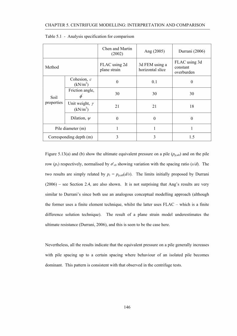
CHAPTER 5. CENTRIFUGE MODELLING: INTERPRETATION AND COMPARISON
146
Table 5.1 - Analysis specification for comparison
Chen and Martin (2002) Ang (2005) Durrani (2006)
Method FLAC using 2d plane strain
3d FEM using a horizontal slice
FLAC using 3d constant overburden
Cohesion, c (kN/m2) 0 0.1 0
Friction angle, 'φ 30 30 30
Unit weight, γ (kN/m3)
21 21 18
Soil properties
Dilation, ψ 0 0 0
Pile diameter (m) 1 1 1
Corresponding depth (m) 3 3 1.5
Figure 5.13(a) and (b) show the ultimate equivalent pressure on a pile (pp,ult) and on the pile
row (pr) respectively, normalised by σ'v0 showing variation with the spacing ratio (s/d). The
two results are simply related by pr = pp,ult(d/s). The limits initially proposed by Durrani
(2006) – see Section 2.4, are also shown. It is not surprising that Ang’s results are very
similar to Durrani’s since both use an analogous conceptual modelling approach (although
the former uses a finite element technique, whilst the latter uses FLAC – which is a finite
difference solution technique). The result of a plane strain model underestimates the
ultimate resistance (Durrani, 2006), and this is seen to be the case here.
Nevertheless, all the results indicate that the equivalent pressure on a pile generally increases
with pile spacing up to a certain spacing where behaviour of an isolated pile becomes
dominant. This pattern is consistent with that observed in the centrifuge tests.

CHAPTER 5. CENTRIFUGE MODELLING: INTERPRETATION AND COMPARISON
147
(a) Plane strain model (after Chen and Martin, 2002)
(b) Three-dimensional horizontal slice model (after Ang, 2005)
Figure 5.12 - Boundary conditions of 2d and 3d numerical models used
Upslope Downslope
PileForced displacement
Forced displacement
Pile (d = 1m)
Upstream
Downstream s/2
Top surface
Bottom

CHAPTER 5. CENTRIFUGE MODELLING: INTERPRETATION AND COMPARISON
148
0
2
4
6
8
10
12
0 1 2 3 4 5 6 7 8 9 10 11 12
Ulti
mat
e eq
uiva
lent
pile
pre
ssur
e , p
p,ul
t/ σ
' v0
s / d
Isolated pile, Kp2
Continuous wall,(Kp - Ka)(s/d)
Durrani (2006)
Chen and Martin (2002)
Ang (2005)
Factored limit, Kp
(a) Ultimate equivalent pile pressure (equivalent to Bmob)
0
0.5
1
1.5
2
2.5
3
3.5
0 1 2 3 4 5 6 7 8 9 10 11 12Equi
vale
nt a
vera
ge p
ress
ure a
long
the
pile
row
,p r
/ σ' v0
s / d
Isolated pile, Kp2 (d/s)
Continuous wall, Kp - Ka
Factored limit, Kp (d/s)
Durrani (2006)
Ang (2005)
Chen and Martin (2002)
(b) Equivalent average pressure along the pile row
Figure 5.13 - Ultimate equivalent pressures on a pile and on a pile row with theoretical
limits
CHAPTER 5. CENTRIFUGE MODELLING: INTERPRETATION AND COMPARISON
149
5.4.3 Davies et al. (2003)
The reference is based on stabilisation works for a large slip on a Southerly section of the
M25, Surrey. ‘Section C’ which is the area of the greatest apparent movement will be
considered (Figure 5.14(a)).
A translational failure slip (approximately parallel to a slope surface, inclined at 11° to 15° to
the horizontal) was developed between 8 – 10 m depth below ground level, extending from a
steep backscarp about 80 m up the slope, down to the motorway hard shoulder. The slip was
within weathered or unweathered Gault clay, with overlying head deposits covering the
upper portion of the slope (Figure 5.14(b)). Properties of soils comprising of the slope are
given in Table 5.2.
Table 5.2 - Geotechnical material properties
Design parameters Other properties c' 'φ cu PI W/C Material
kPa kPa
Head 0 14 50 40
Gault clay 1 24 100 45 35
Residual Gault clay 0 14 50
The lowest FoS for Section C obtained using a slip circle method (Slope/W software) was
0.93. The pile row was designed to provide an additional stabilising force required for 20%
increase in the FoS, based in part on Viggiani’s method (see Chapter 2).
The total weight of the unstable material upslope of the pile row can be estimated as about
γlh = 20 × 50 × 8 = 8,000 kN/m (see Figure 5.14(b)), with a ‘driving’ component acting
down the failure surface of about 8,000 × sin11° = 1,500 kN/m. The stabilising force used
CHAPTER 5. CENTRIFUGE MODELLING: INTERPRETATION AND COMPARISON
150
(Figure 5.14(c)) was 250 kN/m, which corresponds to about 250 / 1500 × 100 % = 17 % of
the driving force, and is thus broadly consistent with a 20 % increase in FoS.
A row of discrete bored piles (1.05 m diameter and 16 m long) was installed at (s/d) = 2.5,
and positioned at approximately one third of the way up the failure (25m from the back of
the motorway kerb). In order to give an additional enhancement of stability, a drainage
system was designed to reduce the groundwater level.
The following properties were used for comparison:
• passive earth pressure Kp = (1+sin 'φ ) / (1-sin 'φ ) = 2.37 for 'φ = 24° (taking
standard soil strength for the soil above the residual shear surface)
• active earth pressure Ka = (1-sin 'φ ) / (1+sin 'φ ) = 0.42
• groundwater level after drainage installation hw = 3 m above the slip
For stability of the slope the total stabilising force for n piles across the width b (Equation
(5.11) is slightly modified to include the effect of the pore water pressure u due to the
groundwater above a slip):
2p mob u
1 (1 )2
S nS B r h ndγ= = − (5.24)
where ru is the pore pressure ratio that (the ratio of the pore water pressure to the total
vertical stress). At the slip surface ru = u/(γh) = (γwhw)/(γh) = (10×3)/(20×8) = 0.2. In fact ru
varies with depth, but this value will be considered representative for the entire depth, and is
slightly conservative since it is actually the maximum value over this depth provided the
drainage remains effective.

CHAPTER 5. CENTRIFUGE MODELLING: INTERPRETATION AND COMPARISON
151
The equivalent stabilising force per unit width along the pile row due to passive interaction is
derived by dividing by b = ns, and is required to be 250 kN/m (as above):
2mob u
1ˆ (1 )2
S S dS B r hb ns s
γ= = = − = 250 kN/m (5.25)
Hence Bmob = 250×2/{(1-0.2)×20×82×(1/2.5)} = 1.2. This value is plotted in Figure 5.15,
which also shows the critical pile spacing, and the ‘unfactored’ (Kp2) and ‘factored’ (Kp)
limits on interaction pressure for individual piles. The spacing is slightly less than the
critical value, and quite significantly less than the factored limit on interaction pressure. The
impact of passive limiting drained interaction on the stability was not considered in the
design (since this effect was not reflected in Viggiani’s method which was used), and thus
this results in excessively over-conservative design from the perspective of pile soil
interaction (but not necessarily structural capacity etc). Thus it appears that the proposed
design is much more robust in this respect so that it can potentially be used to assess the
effect of pile spacing for a given load in practice.

CHAPTER 5. CENTRIFUGE MODELLING: INTERPRETATION AND COMPARISON
152
(a) Geomorphological map
(b) Schematic layout of cross-sectional plane section
(c) Stabilising force versus improved factor of safety
Figure 5.14 - Geomorphological mapping and schematic layout (after Davies et al., 2003)
Idealised shear surface
10 m 8 m
d = 1.05 m, s/d = 2.5
Recorded winter conditions
No working drainage (Slope/W)
Working drainage (Slope/W)
5 m
l = 50 m 25 m
γ = 20 kN/m3
5 m

CHAPTER 5. CENTRIFUGE MODELLING: INTERPRETATION AND COMPARISON
153
0
1
2
3
4
5
6
7
8
0 1 2 3 4 5 6 7 8
B mob
s / d
Isolated pile, Bmax = Kp2
Continuous pile wall, (Kp-Ka)(s/d)
Bmob = Kp
Design
(s/d)crit
Figure 5.15 Comparison of Bmob with the ‘factored’ and ‘unfactored’ theoretical limits

CHAPTER 5. CENTRIFUGE MODELLING: INTERPRETATION AND COMPARISON
154
5.5 Summary
Based on analysis of a semi-infinite slope under conditions of plane strain, a theoretical
method has been established for interpreting the centrifuge test data. The proposed method
embodied two important variables A and Bmob as follows:
• loading on the pile row
A is the proportion of the weight of the upslope material loading the pile row
(Equation 5.8). It is related mainly to the inclination of the pre-defined failure
interface, with some reduction due to friction on this interface and the sides of the
plane strain section.
• the corresponding interaction pressure on a pile in the row
Bmob is the corresponding interaction pressure mobilised on a pile, expressed as a
dimensionless factor normalised by the nominal vertical effective stress in the soil at
a given depth (Equation 5.12). This value tends to increase with the weight of the
upslope material, and pile spacing.
The above relationships were compared with the centrifuge test data, and showed very good
correspondence in general:
• The maximum value of A was observed for low (s/d) or (l/h), and corresponded quite
well with the theoretical prediction. The corresponding Bmob was less than the
ultimate interaction pressure. However, A tended to reduce relative to its maximum
value as the limiting interaction pressure was mobilised (i.e. Bmob = Bmax), for higher
(s/d) or (l/h), generally indicating inability of the pile row to maintain stability of the
upslope material, with corresponding significant displacement.

CHAPTER 5. CENTRIFUGE MODELLING: INTERPRETATION AND COMPARISON
155
• The ultimate value of interaction was found to be Bmob = Kp2 as proposed by Fleming
et al. (1982). It could be argued that the limiting interaction pressure would be
increased due to the inclination of the upslope soil loading the piles. However the
limiting value does not appear to be significantly increased, and it is in any case
conservative to ignore this potential effect in design. In the centrifuge tests the
presence of a pre-defined low friction interface meant that this pressure was
observed through the full depth of unstable material as an approximately triangular
distribution. However, in a more general situation the passive pressure is likely to
reduce more gradually to zero at some depth.
• According to numerical analyses conducted by Durrani et al (2006) the Kp2 limit on
interaction (for an isolated pile) could be used to propose a limit on centre-to-centre
spacing (s) where behaviour of the pile row ceases to be a ‘wall’ and becomes more
like individual piles at larger spacing. This limiting interaction pressure was verified
in the tests.
• For a given magnitude of Bmob less than the limiting value the value of (s/d) does not
have significant impact on the corresponding magnitude of relative pile-soil
displacement. This supports another observation by Durrani (2007) that piles spaced
wider than the critical value still offer support to the upslope material – it is just that
the equivalent value per metre along the slope drops in proportion to (1/s) for a given
value of Bmob.
• There was some evidence that for closely spaced piles the reduction in limiting
pressure predicted by Durrani et al (2006) for the ‘wall’ (as opposed to isolated
piles) was observed. It could be argued that greater loading on the pile row would
have been required to prove this conclusively, but the test package would not allow

CHAPTER 5. CENTRIFUGE MODELLING: INTERPRETATION AND COMPARISON
156
this, and in any case there would have been very significant tendency for failure
upslope of the piles, thus limiting interaction with the piles.
Comparison of the centrifuge test results with some of the references reviewed in Chapters 2
was made, focusing on the effect of pile row interaction. Ito and Matsui’s approach did not
give accurate predictions of the ‘full’ ultimate resistance – especially at low (s/d), where the
trend of behaviour is incorrect. However, as above, the references based on numerical
approaches (particularly the ‘constant overburden approach’, Durrani et al, 2006) showed
consistency with the centrifuge test results.
Comparison with a field study indicated that the scheme (which has performed satisfactorily
to date) was designed with an appropriate pile interaction pressure for the desired
improvement in factor of safety.

157
CHAPTER 6
CONCLUSIONS
6.1 Work reported in the thesis
6.1.1 Centrifuge model tests
A total of 23 centrifuge model tests (based on plane strain except the pile row) were
undertaken, modelling a purely frictional slope comprising sliding (unstable) ground and
stable underlying material, separated by the presence of a predefined failure surface. The
predefined surface was a translational slip parallel to the slope surface at 0.07m depth at
model scale, having a very low shear resistance to increase the tendency for the upper
portion of the slope to cause passive loading on the piles over a known depth.
The model piles were installed in a row at a discrete intervals across the slope, with the total
embedded length 205 mm (at model scale) to give sufficient active pile resistance against
lateral passive loading. The pile was instrumented to measure bending moment at ten
locations through its depth. The ground displacements (in the cross sectional plane and of
the slope face), and the pile head displacement, were measured using in-flight photography
and digital image processing (based on GeoPIV). The maximum acceleration used in the
centrifuge tests was 50 g, at which point the thickness of sliding material corresponded to
3.5 m at ‘prototype’ scale, and the pile length was 10.3 m.
The idealised model is intended to investigate the underlying principles controlling passive
stabilisation behaviour at a realistic prototype scale rather than to consider a specific

CHAPTER 6. CONCLUSIONS
158
prototype. The ratio of the upslope length to the thickness of unstable soil (l/h) and the
normalised pile spacing (s/d) were used for this purpose.
Ground and pile head movements during a test were satisfactorily measured via geoPIV
analysis, and ground deformation features were characterised by combination of the ratios
(l/h) and (s/d):
• the ground and pile head displacements, and relative pile-soil displacement, tend to
increase with (s/d) for a given (l/h), and for a given (s/d) displacements also tend to
increase with (l/h)
• upslope failure with a ‘passive wedge’ at large (l/h) and small (s/d)
• flow through the piles with significant deformation at large (l/h) and (s/d)
• a stable condition with small deformation at small (l/h) and (s/d)
• shallow surface failure passing through the piles at small (l/h) and large (s/d)
Back analysis of bending moment data was largely successful in deriving distributions of
shear force and lateral pressure, using a number of curve-fitting techniques:
• the bending moment increases with depth until a maximum in the active zone is
reached where shear force is zero
• the pressure in the passive zone increases approximately linearly with depth and
shows a maximum value at the predefined slip depth. This observation is related to
the imposition of the low friction pre-defined slip. In a more general situation the
passive pressure would probably reduce more gradually to zero at some depth.
• the passive pressure is actively resisted in the stable ground, with a point of pressure
reversal in the active zone to give moment equilibrium of the pile

CHAPTER 6. CONCLUSIONS
159
6.1.2 Analytical model
An approximate analytical model (based on a limit equilibrium method) was developed to
enhance generic understanding of slope stabilisation using a row of piles, and particularly to
allow interpretation of the centrifuge test results, based on:
• The stabilising force required for the unstable material depending on (1) the mass of
the soil upslope of the pile row, (2) the inclination of the predefined failure surface,
and some adjustment for friction on the failure surface and sides of the model.
• The amount of passive interaction for the pile row corresponding to the above
loading.
The proposed method gave a logical framework for interpretation of the data, and showed
good correspondence with the centrifuge test results.
6.2 Implications for design
• The ultimate value of interaction was found to be Bmob = Kp2 as proposed by
Fleming et al. (1982). It could be argued that the limiting interaction pressure
would be increased due to the inclination of the upslope soil loading the piles.
However the limiting value does not appear to be significantly increased, and it is in
any case conservative to ignore this potential effect in design. In the centrifuge tests
the presence of a pre-defined low friction interface meant that this pressure was
observed through the full depth of unstable material as an approximately triangular
distribution. However, in a more general situation the passive pressure is likely to
reduce more gradually to zero at some depth.

CHAPTER 6. CONCLUSIONS
160
• According to numerical analyses conducted by Durrani et al (2006) the Kp2 limit on
interaction (for an isolated pile) could be used to propose a limit on centre-to-centre
spacing (s) where behaviour of the pile row ceases to be a ‘wall’ and becomes more
like individual piles at larger spacing. This limiting interaction pressure was verified
in the tests, and hence the following relationship;
2p
crit p a
Ksd K K
⎛ ⎞ =⎜ ⎟ −⎝ ⎠ (5.14)
• For a given magnitude of Bmob less than the limiting value the value of (s/d) does not
have significant impact on the corresponding magnitude of relative pile soil
displacement. This supports another observation by Durrani (2006) that piles spaced
wider than the critical value still offer support to the upslope material – it is just that
the equivalent value per metre along the slope drops in proportion to (1/s) for a given
value of Bmob.
• There was some evidence that for closely spaced piles the reduction in limiting
pressure predicted by Durrani et al (2006) for the ‘wall’ (as opposed to isolated
piles) was observed. It could be argued that greater loading on the pile row would
have been required to prove this conclusively, but the test package would not allow
this, and in any case there would have been very significant tendency for failure
upslope of the piles, thus limiting interaction with the piles.
Comparison of the centrifuge test results with some of the references reviewed in Chapter 2
was made, focusing on the effect of pile row interaction. Ito and Matsui’s approach did not
give accurate predictions of the ‘full’ ultimate resistance – especially at low (s/d), where the
trend of behaviour is incorrect, which does not give confidence in the use of this approach.
Wang and Yen’s approach relies on specifying uncertain geometrical parameters, and there

CHAPTER 6. CONCLUSIONS
161
is no dependency on pile diameter, so the use of this approach is not recommended in
practical design. However, as above, the references based on numerical approaches
(particularly the ‘constant overburden approach’, Durrani et al, 2006) showed consistency
with the centrifuge test results.
6.3 Recommendations for future work
Recent numerical modelling (Durrani 2006) improved generic understanding of interaction
for a passively loaded pile row, and this work has now been supplemented and confirmed by
physical modelling in a geotechnical centrifuge. Areas for further work mainly consider
more detailed aspects of behaviour associated with design in specific circumstances; for
instance movement of soil and piles. These areas are generally complicated by the inherent
assumptions made in design, such as calculating displacements which are associated with a
factor of safety for the slope which is in excess of 1.0, and therefore arguably not relevant to
a serviceability calculation. Nevertheless some areas where further work could be
undertaken are listed below:
• Horizontal restraint at the pile head can have significant benefit in reducing bending
moments in the pile and corresponding displacement. However, there is not likely to
be significant effect on the limiting interaction pressure derived from this work.
• The effect of orientation or multiple rows of piles (e.g. miniplies) in a slope could be
investigated – particularly with regard to the limiting interaction pressure.
• Use of a lower slope angle compared to the soil friction angle would reduce potential
issues with shallow surface failures, also improving PIV on the face of the slope.
• The impact of flexibility of the piles or active behaviour depending on the embedded
depth below a slip could be examined. However, such aspects of behaviour are
closely related to the wider study of laterally loaded piles.
CHAPTER 6. CONCLUSIONS
162
• Relative pile-soil displacement in relation to Bmob was considered in Chapter 5, but
the movement cannot be interpreted directly as equivalent prototype values since it
accumulated at a variety of g-levels. This aspect of behaviour could be studied in
more detail.

163
APPENDIX
A. Derivation of pile displacement profile with depth
Figure A.1 shows general sign conventions and notation for displacement and rotation of a
pile, where subscript ‘i’ denotes the position of an interface and ‘l1’ is the distance from a
pile tip to a point of pressure reversal. Rotation (θ) is positive in the anticlockwise and
downslope displacement (u) of a pile is positive (see Figure 4.1)
Figure A.1 General definitions and conventions for pile rotation and displacement
Interface
l1
zb,i Point of pressure reversal
za,i Sliding direction za
zb
Pressure distributions
Initial position of a pile
Deformed position of a pile

APPENDIX A. DERIVATION OF PILE DISPLACEMENT PROFILE WITH DEPTH
164
The pile displacement profile with depth can be derived by integrating the moment
polynomials twice, as follows:
1. Passive zone (based on P2 approach)
3 4
1 2( )6 12a a
az zM z a a= + (A1a)
4 5
1 2 10
1( ) ( )24 60
aza a
a a az zz M z dz a a A
EIθ
⎛ ⎞= = + +⎜ ⎟
⎝ ⎠∫
1a Aθ= + (A1b)
5 6
1 2 1 20
1( ) ( )120 360
aza a
a a a az zu z z dz a a A z A
EIθ
⎛ ⎞= = + + +⎜ ⎟
⎝ ⎠∫
1 2a au A z A= + + (A1c)
2. Active zone (based on P3 approach)
2 3 4
0 1 2( )2 6 12b b b
bz z zM z b b b= + + (A2a)
3 4 5
0 1 2 10
1( ) ( )6 24 60
bzb b b
b b bz z zz M z dz b b b B
EIθ
⎛ ⎞= = + + +⎜ ⎟
⎝ ⎠∫
1b Bθ= + (A2b)
4 5 5
0 1 2 1 20
1( ) ( )24 120 360
bzb b b
b b b bz z zu z z dz b b b B z B
EIθ
⎛ ⎞= = + + + +⎜ ⎟
⎝ ⎠∫
1 2b bu B z B= + + (A2c)

APPENDIX A. DERIVATION OF PILE DISPLACEMENT PROFILE WITH DEPTH
165
Assuming the following conditions the total four constants of integration (A1, A2, B1, and B2)
are derived by:
• the pile deflection at the head, u(za,head), is equal to the pile head displacement
measured from image analysis in the test (δp), ,( )a head pu z δ=
2 ,( )a head pA u z δ= =
• continuity of gradient (rotation) at the interface, , ,( ) ( )a i b iz zθ θ=
, 1 , 1 0a i b iA Bθ θ+ + + =
1 , , 1( )a i b iA Bθ θ= − + +
• the point of pressure reversal in the active zone (zb = l1) corresponds to zero absolute
pile deformation, 1,( ) 0b lu z =
1, 1 1 1 2( ) 0b lu z ub B l B= + + =
2 1 1 1( )b bB u B l= − +
• continuity of pile displacement at the interface, , ,( ) ( )a i b iu z u z=
, 1 , 2 , 1 , 2a i a i b i b iu A z A u B z B+ + = + +
1 , , 2 , 1 , 2b i b i a i a iB z u B u A z A= + − − −
1 , , 1 1 1 , , , 1 ,( ) ( )b i b i b a i a i b i a i pB z u u B l u B zθ θ δ= − + − + + + −
1 , 1 , , 1 , , , ,( ) ( )b i a i b i b a i a i b i a i pB z l z u u u zθ θ δ+ − = − − + + −
, , ,, 1 ,1
,1,
( )a i a i a i pb i b b i
a ib i
u u u zB
z l zθ θ δ− − + + −
=+ −
This allows four independent equations to be written in terms of the four unknown constants
of integration. Hence a unique solution exists and can be derived.
166
REFERENCES
Adachi, T., Kimura, M. and Tada, S. (1989). Analysis on the preventive mechanism of
landslide stabilizing piles. 3rd International Symposium on Numerical Models in
Geomechanics , pp. 691-698.
Ang, E. (2005). Numerical investigation of load transfer mechanism in slopes reinforced
with piles. PhD thesis, University of Missouri-Columbia.
Ausilio, E., Conte, E. and Dente, G. (2001). Stability analysis of slopes reinforced with piles.
Computers and Geotechnics , 28, pp. 591-611.
Baguelin, R., Frank, R. and Said, Y.H. (1977). Theoretical study of lateral reaction
mechanism of piles. Geotechnique , 27 (3), pp. 405-434.
Boeckmann, A. (2006). Load transfer in micropiles for slope stabilization from tests of large-
scale physical models. MSc thesis, University of Missouri-Columbia.
Bosscher, P.J. and Gray, D.H. (1986). Soil arching in sandy soil. Journal of Geotechnical
Engineering , 112 (6), pp. 625-645.
British Standard 1377 (1990). Methods of Test for Soils for Civil Engineering Purposes,
British Standard Institution, London.
Broms, B. (1964). Lateral resistance of piles in cohesionless soils. Journal of Soil Mechanics
and Foundation Division , 40 (1), pp. 73-84.

167
Cai, F. and Ugai, K. (2000). Numerical analysis of the stability of a slope reinforced with
piles. Soils and Foundatations , 40 (1), pp. 73-84.
Carder, D.R. and Easton, M.R. (2001). Analysis of performance of spaced piles to stabilise
embankment and cutting slopes. Transport Research Laboratory, TRL Report 493.
Carder, D.R. and Temporal, J. (2002). A review of the use of spaced piles to stabilise
embankment and cutting slopes. Transport Research Laboratory, TRL Report 466.
Chen, C.Y. and Martin, G.R. (2002). Soil-structure interaction for landslide stabilizing piles.
Computers and Geotechnics , 29, pp. 363-386.
Chen, L.T. and Poulos, H.G. (1997). Piles subjected to lateral soil movements. Journal of
Geotechnical and Geoenvironmental Engineering , 123 (9), pp. 820-811.
Chen, L.T., Poulos, H.G., and Hull, T.S. (1997). Model tests on pile group subjected to
lateral soil movement. Soils and Foundations , 37 (1), pp. 1-12.
Cox, C. (2006). Personal communications.
Craig, W. (1984). Installation studies for model piles. Proceeding of a symposium on the
application of centrifuge modelling to geotechnical design, W. Craig (Ed.), Balkema,
Rotterdam, pp. 440-455.
168
Davies, J.P., Loveridge, F.A., Patterson, D., Carder, D.R. and Perry, J. (2003). Stabilization
of a landslide on the M25 Highway London's Main Artery. 12th Pan-American Conference
of Soil and Mechanics and Geotechnical Engineering. Massachusetts Institute of Technology,
Boston.
De Beer, E., and Carpentier, R. (1976). Discussion of “method to estimate lateral force
acting on stabilising piles” by Ito and Matsui, Soils and Foundations, 17 (1), pp. 68-82.
Durrani, I. (. (2007). Numerical modelling of discrete pile rows to stabilise slopes. PhD
thesis, University of Nottingham.
Durrani, I.K., Ellis, E.A. and Reddish, D.J. (2006). Modelling lateral pile-soil interaction for
a row of piles in a frictional soil. 4th International FLAC Symposium on Numerical
Modelling in Geomechanics 2006 ISBN 0-9767577-0-2, pp. 231-238.
Durrani, I.K. (2007). Numerical modelling of discrete pil rows to stabilise slopes. PhD thesis,
the University of Nottingham.
Dyson, G.J. and Randolph, M.F. (1998). Installation effects on lateral load-transfer curves in
calcareous sands. Centrifuge 98. Balkema, Rotterdam.
Ellis, E.A., Cox, C., Yu, H.S., Ainsworth, A. and Baker, N. (2006). A new geotechnical
centrifuge at the University of Nottingham, UK. 6th International Conference of Physical
Modelling in Geotechnics: ICPMG'06. Taylor & Francis Group, London, pp. 129-133.
Fleming, W.G.K., Weltman, A.J., Randolph, M.F. and Elson, W.K. (1994). Piling
engineering. Taylor & Francis Books Ltd.

169
Foray, P., Balachowski, L. and Rault, G. (1998). Scale effect in shaft friction due to the
localisation of deformations. Centrifuge'98. Balkema, Rotterdam.
Garnier, J. and Konig, D. (1998). Scale effects in piles and nails loading tests in sand.
Centrifuge'98. Balkema, Rotterdam.
Gui, M.W. and Bolton, M.D. (1998). Geometry and scale effect in CPT and pile design.
Geotechnical Site Characterization. Balkema, Rotterdam.
Hassiotis, S., Chameau, J.L. and Gunaratne, M. (1997). Design method for stabiliization of
slopes with piles. Journal of Geotechnical and Geoenvironmental Engineering , 123 (4), pp.
314-323.
Hayward, T., Lees, A., Powrie, W., Richards, D.J. and Smethurst, J. (2000). Centrifuge
modelling of a cutting slope stabilised by discrete piles. Transport Research Laboratory,
TRL Report 471.
Ito, T. and Matsui, T. (1975). Methods to estimate lateral force acting on stabilising piles.
Soils and Foundations , 15 (4), pp. 43-59.
Jeong, S., Kim, B., Won, J. and Lee, J. (2003). Uncoupled analysis of stabilising piles in
weathered slopes. Computers and Geotechnics , 30, pp. 671-682.
Kulhawy, F.H. (1991). Drilled shaft foundations. Foundation engineering book, 2nd eds.
Chap. 14. H.Y. Fang (Ed)., Van Nostrand Reinhold, New York.
Lee, C.Y., Hull, T.S. and Poulos, H.G. (1995). Simplifed pile-soil stability analysis.
Computers and Geotechnics , 17, pp. 1-16.

170
Liang, R. and Zeng, S. (2002). Numerical study of soil arching mechanism in drilled shafts
for slope stabilisation. Soils and Foundations , 42 (2), pp. 83-92.
Lyndon, A. and Pearson, R.A. (1988). Skin friction effects on laterally loaded large diameter
piles in sand. Centrifuge 88. Balkema, Rotterdam, pp. 363-370.
Perry, J., Pedley, M. and Brady, K. (2003a). Infrastructure cuttings - condition appraisal and
remedial treatment. CIRIA Report C591.
Perry, J., Pedley, M., Reid, M. (2003b). Infrastructure embankments - condition appraisal
and remedial treatment. CIRIA Report C592.
Poulos, H. (1999). Design of slope stabilising piles. Research Report. University of Sydney,
Department of Civil Engineering.
Poulos, H.G., Chen, L.T. and Hull, T.S. (1995). Model tests on single piles subjected to
lateral soil movement. Soils and Foundations , 35 (4), pp. 85-92.
Schofield, A. (1980). Cambridge geotechincal centrifuge operations: 20th Rankine lecture.
Geotechnique , 30 (2), pp. 129-170.
Smethurst, J.A. and Powrie, W. (2007). Monitoring and analysis of the bending behaviour of
discrete piles used to stabilise a railway embankment. Geotechnique , 57 (8), pp. 663-677.
Takemura, J. (1998). In K. a. Kimura (Ed.), Centrifuge 98, Balkema, Rotterdam. pp. 1087-
1123.

171
Taylor, R. (1995). Geotechnical Centrifuge Technology. Blackie Academic & Professional.
Thompson, M.J. and White, D.J. (2006). Design of slope reinforcement with small diameter
piles. In J. Y. Han (Ed.), Proceedings of sessions of GeoShanghai 2006: Advances in Earth
Structure: Research to Practice. ASCE, GSP151. pp. 67-73
Viggiani, C. (1981). Ultimate lateral load on piles used to stabilize landslids. Proceeding of
10th European Conference on Soil Mechanics and Foundation Engineering, 3, pp. 555-560.
Wang, W.L. and Yen, B.C. (1974). Soil arching in slopes. Journal of Geotechnical
Engineering Division , 100, pp. 61-78.
White, D.J., Take, W.A. and Bolton, M.D. (2003). Soil deformation measurement using
particle image velocimetry (PIV) and photogrammetry. Geotechnique , 53 (7), pp. 619-631.
Won, J., You, K., Jeong, S., and Kim, S. (2005). Coupled effects in stability analysis of pile-
slope systems. Computers and Geotechnics , 32, pp. 304-315.