yhklfoh - eucass

8th

European conference for aeronautics and space sciences (EUCASS)

Copyright 2019 by Thibault CANTOU, Nicolas MERLINGE, and Romain WUILBERCQ. Published by the

EUCASS association with permission.

3DoF simulation model and specific aerodynamic control

capabilities for a SpaceX’s Starship-like atmospheric reentry

vehicle

Thibault CANTOU*, Nicolas MERLINGE**, Romain WUILBERCQ***

*ONERA – DTIS – NGPA

[email protected]

**ONERA – DTIS – CEVA

[email protected]

***ONERA – DTIS – CEVA

[email protected]

Abstract In September 2018, a novel design of reusable atmospheric reentry vehicle was proposed: SpaceX’s

Starship (SXS). Its main difference with comparable vehicles lays in its aerodynamic actuators that

allow for stable flight at angles of attack (AoA) up to 90°. In this work, we propose a 3DoF simulation

model of this vehicle, and present preliminary reentry simulation results. A study of the center of mass

location’s implications on longitudinal stability is presented. The modulation of the aerodynamic

forces at a given equilibrium AoA allowed by the multiactuator configuration is discussed and

demonstrated on a reentry trajectory simulation.

1. Introduction

Since the beginning of the space era, the design of vehicles able to survive atmospheric reentry has been a

challenging engineering problem. Reentry at orbital or near-orbital velocity implies very intense heat, aerodynamic

pressure, and load factor. These issues are tackled with a combination of careful vehicle design (heat shielding or

regenerative cooling, tough structure, etc.), and careful mission planning through reentry trajectory optimization if

the vehicle has a maneuvering capability.

The reentry trajectory can be divided in two phases: the exo-atmospheric phase, and the atmospheric phase. The

latter is the most constraining one due to aerodynamic and aero-thermal effects at high velocity. During the first

phase, the trajectory is controlled by exerting thrusts in various directions to track a desired velocity vector

(orientation and norm). During the second phase, vehicles will often exploit angle of attack (AoA) and bank angle

(BA) control to manoeuver and track a reference constrained trajectory minimizing heating, load factor, and

aerodynamic pressure.

Atmospheric trajectory optimization relies a lot on the aerodynamic capabilities of the considered vehicle. The first

generations of reentry vehicles (i.e. reentry capsules) needed to be simple, robust to a great amount of uncertainties,

and small enough to fit in the rockets of that era. The geometry allowing to deal with those constraints with the

technology available at that time was not in favor of a high lift-to-drag ratio vehicles. They were nevertheless

somewhat maneuverable during the atmospheric part of the flight (AoA and BA) thanks to center-of-mass (CoM)

location control and/or cold gas thrusters for attitude control.

Later, technological progress and the need for reusability allowed the design of rather safe reentry vehicles with more

aerodynamically efficient shapes (i.e. with higher lift-to-drag ratio). The Space Shuttle and the X37-B are great

examples of such vehicles. Their actuators (similar to those of an aircraft) allow this category of vehicle to remain

stable at high AoA during the atmospheric flight. This then generate lift that can be oriented through BA control and

used to shape the trajectory as needed.

The subject of this study, a novel design for a reusable atmospheric reentry vehicle, was proposed in September

2018: Space X’s Starship (SXS). It exhibits an innovative configuration of aerodynamic control surfaces granting it

unique capabilities. The motivation for this work is to give elements to understand why this configuration is an

interesting choice. In the following sections, we will:

DOI: 10.13009/EUCASS2019-337

Thibault CANTOU, Nicolas MERLINGE, Romain WUILBERCQ

2

Propose an OpenVSP [1] geometrical model of SpaceX’s Starship;

Introduce the methodology used to generate an aerodynamic database for lift, drag, and pitching moment at

hypersonic speeds;

Analyze the implications of this design on longitudinal aerodynamic stability and its dependency to the

location of the center of mass ;

Discuss the implication of the multi-actuator configuration on aerodynamic forces modulation while holding

the vehicle at a fixed angle of attack ;

Provide some atmospheric reentry simulation results to illustrate the performances of the vehicle.

2. Context

SXS will be the second stage of SpaceX’s future heavy rocket. It will be mounted on top of the Super Heavy booster.

As it is a reusable second stage, SXS needs propulsion in order to reach the orbit, deorbit itself, and achieve a

propulsive landing. But it also needs actuators able to control its attitude during atmospheric reentry. Since this study

is focused on the behavior of SXS in the hypersonic regime during its reentry, it does not integrate a propulsive

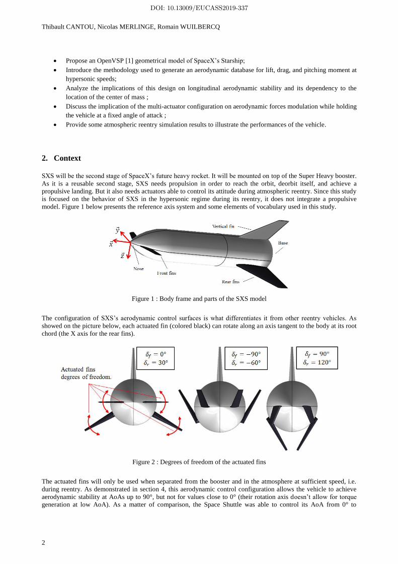
model. Figure 1 below presents the reference axis system and some elements of vocabulary used in this study.

Figure 1 : Body frame and parts of the SXS model

The configuration of SXS’s aerodynamic control surfaces is what differentiates it from other reentry vehicles. As

showed on the picture below, each actuated fin (colored black) can rotate along an axis tangent to the body at its root

chord (the X axis for the rear fins).

Figure 2 : Degrees of freedom of the actuated fins

The actuated fins will only be used when separated from the booster and in the atmosphere at sufficient speed, i.e.

during reentry. As demonstrated in section 4, this aerodynamic control configuration allows the vehicle to achieve

aerodynamic stability at AoAs up to 90°, but not for values close to 0° (their rotation axis doesn’t allow for torque

generation at low AoA). As a matter of comparison, the Space Shuttle was able to control its AoA from 0° to

DOI: 10.13009/EUCASS2019-337

3DoF simulation model and specific aerodynamic control capabilities for a Space X’s Starship-like atmospheric

reentry vehicle.

3

approximately 40°. This very high AoA stability provides SXS with different manœuvering capabilities that need to

be explored.

3. SXS Model creation 3.1. 3D geometry of the vehicle in OpenVSP

The 3D geometry of the vehicle was created in NASA’s OpenVSP [1] from photographs. As the vehicle is still in

active development, the precise three-dimensional shape varies from a published picture to another. Therefore a

representative model of the aerodynamic configuration of SXS has been created rather than a picture perfect model.

As stated on SpaceX’s website [2], the vehicle’s diameter is 9 m, and its length is 55 m including the fins. This

allowed us to infer the rest of the required dimensions.

Body:

The body is 51 m long. The ogive section ends at 13 m along the X axis from the nose and then blends into a

cylindrical shape until the base of the vehicle.

Actuated fins:

The selected profile is a symmetrical NACA 0010 profile. The planform is modelled the following way:

Front fins: The front point of the front fins is located 2.6 m rearward the nose on the X axis. At the root,

their chord is 3.5 m. At the tip, it is 2.2 m. The section tangent to the body forms an angle of 22° around

the Z axis. They span 3 m orthogonally to the first section. The taper ratio is 0.63 and the sweep angle

is 30°. The dihedral angle is the control angle and is limited to the range [-90°, 90°].

Rear fins: The front point of the rear fins is located 37.8 m rearward the nose on the X axis, at an angle

of 30° down the XY plane. At the root, their chord is 11.4 m. At the tip, it is 3.7 m. They span 6.2 m

orthogonally to the first section. The sweep angle is 64°. The dihedral angle is the control angle and is

limited to [-60°, 120°].

Vertical fin:

It is similar to the rear fins but the dihedral angle is kept at -90°.

Figure 3 : Up view (left) and right-side view (right) of the OpenVSP model

The convention for the fins control angles is chosen negative up and positive down. To account for the dependency

of the aerodynamics to the actuated fins angles, a set of 3D models has been generated for every combination of rear

and front fins angles in their respective definition domain with a step angle of 10°. From each of these models, a 3D

mesh has been created in OpenVSP and then used in SHAMAN, as described over the next section.

3.2. Reduced-Order Hypersonic Aerodynamics

Future reusable launchers, such as those of interest in the present study, will face some severe aero-thermodynamic

loads during their reentry into the terrestrial atmosphere. They will travel from the near-vacuum conditions of space -

i.e. in the free-molecular flow regime - to the denser region of the lower atmosphere - i.e. in the continuum flow

regime – and through a mixed-density transitional flow regime in between.

In the context of this study however, since the reentry trajectory of the Starship occurs mostly in regions where the

flow behaves as a continuum, it is assumed that methods that are valid in this regime can be applied throughout the

flight envelop of the vehicle.

An in-house code, dubbed Shaman, is thus used in order to quantify the inviscid aerodynamics of our vehicle when it

operates in the realm of the hypersonic flow regime. Shaman embeds a number of simplified methods, the so-called

DOI: 10.13009/EUCASS2019-337


4

Local Surface Inclination (LSI) methods [3]. Those only require, as inputs, a triangulation to describe the geometry

of the vehicle being modelled (see Figure 4 below), the local inclination angle of all surface panels and the

freestream conditions.

Figure 4 : Unstructured triangular mesh of the Starship (made up of 16800 panels)

The decrease in terms of physical realism that accompanies this panel-based approach, especially when compared to

modern numerical methods such as Computation Fluid Dynamics (CFD), is offset almost entirely in many practical

applications by its low computational cost and parametric flexibility [4]. Thus, albeit these LSI methods are

considered of a low fidelity level, they provide reasonable estimates with regard to the preliminary nature of the

analyses presented in this study.

Since the vehicle holds a very high angle-of-attack throughout its reentry trajectory and due to the general bluntness

of the Starship, the modified Newtonian theory has been applied to all parts of the configuration geometry.

Assuming a so-called Newtonian flow, the pressure exerted on the vehicle is thus considered solely due to the total

loss of momentum of the fluid in the direction normal to the vehicle’s surface [3]. The local pressure coefficient

𝐶𝑝,𝑖 at any panel 𝑖 is then given by:

𝐶𝑝,𝑖 = 𝐶𝑝,𝑚𝑎𝑥 sin2 𝜃𝑖 (1)

Where 𝜃𝑖 is the local inclination angle between the freestream flow direction and a tangent to the local surface panel.

As suggested by the work of Lester Lees [5], the modified Newtonian theory accounts for the total pressure loss

across the normal shock that is located ahead of the vehicle. Therefore, 𝐶𝑝,𝑚𝑎𝑥 is equal to the pressure coefficient at

the stagnation point behind a normal shock.

A database of aerodynamic coefficients (i.e. 𝐶𝐿, 𝐶𝐷 and 𝐶𝑚/𝑟𝑒𝑓) has then been created as a function of the freestream

Mach number 𝑀∞ (from Mach 4 to Mach 30), the vehicle’s angle-of-attack 𝛼 (from 0° to 180°), and the front and

rear control fins angles (respectively from -90° to 90°, and from -60° to 120°). Some results from the aerodynamic

database without any deflection of the control surfaces (𝛿 = 0°) are presented in Figure 5.

The aerodynamic coefficients can then be interpolated in order to provide estimates at any particular point along the

trajectory profile through the use of the reference properties associated with our SXS configuration (𝑆𝑟𝑒𝑓 and 𝐿𝑟𝑒𝑓)

and the dynamic pressure. These reference quantities are provided in Table 1. It shall finally be borne in mind that

viscous effects have been neglected in this preliminary work.

Table 1 : Reference Properties for the Aerodynamics of the Starship

Reference Value Remark

Length, 𝑳𝒓𝒆𝒇 [𝒎] 9 Fuselage Diameter

Area, 𝑺𝒓𝒆𝒇 [𝒎𝟐] 64 Fuselage Circular Cross-Section

Reference Point for Moments [𝒎] [-25, 0, 0] The origin is located at the nose of the vehicle

DOI: 10.13009/EUCASS2019-337


reentry vehicle.

5

Figure 5 : Aerodynamic Coefficients at 𝛿𝑟 = 0° and 𝛿𝑓 = 0°

DOI: 10.13009/EUCASS2019-337


6

The aerodynamic forces and moment in wind axis are to be computed with the following expressions:

𝐹𝐿𝑖𝑓𝑡 = − 𝑄. 𝑆𝑟𝑒𝑓. 𝐶𝐿 (2)

𝐹𝐷𝑟𝑎𝑔 = − 𝑄. 𝑆𝑟𝑒𝑓. 𝐶𝐷 (3)

𝑀𝑃𝑖𝑡𝑐ℎ = 𝑄. 𝑆. 𝑙. 𝐶𝑚/𝑟𝑒𝑓 (4)

In the body axis system, the vector forces’ expressions are:

𝐹𝐴𝑥𝑖𝑎𝑙⃗⃗ ⃗⃗ ⃗⃗ ⃗⃗ ⃗⃗ ⃗⃗ = − 𝑄. 𝑆𝑟𝑒𝑓 . 𝐶𝐴. 𝑥 (5)

𝐹𝑁𝑜𝑟𝑚𝑎𝑙⃗⃗ ⃗⃗ ⃗⃗ ⃗⃗ ⃗⃗ ⃗⃗ ⃗⃗ ⃗⃗ = − 𝑄. 𝑆𝑟𝑒𝑓 . 𝐶𝑁 . 𝑧 (6)

With:

𝐶𝐴 = 𝐶𝐷 . cos(𝛼) − 𝐶𝐿 . sin (𝛼) (7)

𝐶𝑧 = 𝐶𝐷. sin(𝛼) + 𝐶𝐿 . cos (𝛼) (8)

3.3. Mass and center of mass

The vehicle’s dry mass is estimated to be 85 tons [6]. The simulation results displayed in section 6 are based on this

dry mass hypothesis, although this value excludes the fuel needed for the landing burn. A study including a

propulsive model would be needed to estimate the required fuel mass needed for this part of the flight and then use a

more representative mass during reentry simulation.

As demonstrated in the next section, the location of the center of mass has a great influence on the AoA solution for

the pitch moment equation equilibrium. We assume that its coordinates in Y and Z are 0, and will only study the

influence of variations of its X coordinate. Since the engines have a significant mass, and that most of the fuel has

already been burnt before its reentry, the CoM is likely to be closer to the base than to the nose of the vehicle along

the X axis. In the next section, we will study aerodynamic stability depending on the CoM’s location. In section 6,

the CoM will be considered still in the body frame and located 30 m behind the nose of the vehicle on the X axis.

4. Pitch equilibrium analysis and sensitivity to CoM location 4.1. Coefficient of moment at CoM

In order to study the influence of the CoM’s location on the pitch equilibrium of the vehicle, the

aerodynamic moment is expressed at the center of mass location (˄ being the cross-product operator):

𝑀𝐶𝑜𝑀⃗⃗ ⃗⃗ ⃗⃗ ⃗⃗ ⃗⃗ = 𝑀𝐶𝑅𝑀⃗⃗ ⃗⃗ ⃗⃗ ⃗⃗ ⃗⃗ ⃗ + (𝐶𝑅𝑀⃗⃗ ⃗⃗ ⃗⃗ ⃗⃗ ⃗ − 𝐶𝑜𝑀⃗⃗⃗⃗⃗⃗ ⃗⃗ ⃗) ∧ 𝐹𝑎𝑒𝑟𝑜⃗⃗ ⃗⃗ ⃗⃗ ⃗⃗ ⃗ (9)

Given that this model is contained in the XZ plan, in the body frame the previous equation becomes:

𝑀𝐶𝑜𝑀⃗⃗ ⃗⃗ ⃗⃗ ⃗⃗ ⃗⃗ |𝑏𝑜𝑑𝑦

= 𝑄. 𝑆. 𝑙. 𝐶𝑚𝐶𝑅𝑀 . 𝑦 + (𝑋𝐶𝑅𝑀 − 𝑋𝐶𝑜𝑀

00

) ∧ (−𝐶𝐴0

−𝐶𝑁)

(10)

With 𝑀𝑌𝐶𝑜𝑀 being the second component of the total aerodynamic moment in the body frame, we have:

𝑀𝑌𝐶𝑜𝑀 = 𝑄. 𝑆. (𝑙. 𝐶𝑚𝐶𝑅𝑀 + (𝑋𝐶𝑅𝑀 − 𝑋𝐶𝑜𝑀). 𝐶𝑁) (11)

DOI: 10.13009/EUCASS2019-337


reentry vehicle.

7

𝑀𝑌𝐶𝑜𝑀 = 𝑄. 𝑆. 𝑙. 𝐶𝑚𝐶𝑜𝑀 (12)

With 𝐶𝑚𝐶𝑜𝑀:

𝐶𝑚𝐶𝑜𝑀 = 𝐶𝑚𝐶𝑅𝑀 +𝑋𝐶𝑅𝑀 − 𝑋𝐶𝑜𝑀

𝑙. 𝐶𝑁

(13)

𝐶𝑚𝐶𝑜𝑀 is a function of Mach, AoA, CoM location, 𝛿𝑟, and 𝛿𝑓. Solving for the AoA, the zeros of 𝐶𝑚𝐶𝑜𝑀 are the

equilibrium points of the pitching moment equation. Moreover, an equilibrium point is open-loop locally stable if the

slope of 𝐶𝑚𝐶𝑜𝑀 is negative. For safety reasons, open-loop rotational stability of the vehicle during atmospheric

reentry is a desirable behavior.

4.2. 𝑪𝒎𝑪𝒐𝑴 VS Mach

In this paragraph, the CoM is considered located at -27.5 m on the X axis. The following curves show the evolution

of 𝐶𝑚𝐶𝑜𝑀 against AoA for several Mach values, and for two sets of fins angles : 0° both (fins parallel to the XY

plan), and -90° front and -60° rear (maximum fins angle above the XY plan, cf. middle picture of Figure 2):

Figure 6 : Variation of 𝐶𝑚𝐶𝑜𝑀 versus Mach number for a CoM located at -27.5 m on the X axis

In the left case, each curve crosses 0 with a negative slope between 32,5°+/-0,5°. In the second one, each curve

crosses 0 between 70°+/-0,5°. These results show that the Mach number has little effect on the value of equilibrium

AoA, but also on the overall values of 𝐶𝑚𝐶𝑜𝑀. This means that the conclusions we can draw at a given point of the

flight domain are valid on the whole Mach number domain. However, this is true only for the study of the

stabilized/final values of the open-loop. The dynamical characteristics of the open-loop remain very dependent on the

Mach number because of the dynamic pressure.

4.3. 𝑪𝒎𝑪𝒐𝑴VS CoM location

In this paragraph, we focus on the sensitivity of the pitching moment to the location of the CoM. In order to reduce

the complexity of the analysis, we will only consider the two following extreme configurations of the fins angles (i.e.

negative values of the angles):

The first configuration is when the rear fins are at 0° (maximally exposed to the airflow) and the front fins

are at 90° up (minimally exposed to the airflow). This configuration corresponds to the case of lowest

equilibrium AoA. The rear fins act like the pitch stabilizers of an airplane’s tail (cf. blue curve on Figure 7).

DOI: 10.13009/EUCASS2019-337


8

The second configuration is the opposite: the rear fins are at 60° up (minimally exposed to the airflow) and

the front fins are at 0° (maximally exposed to the airflow). This corresponds to the case of highest

equilibrium AoA (cf. orange curve on Figure 7).

We deliberately limit the control fins angles to the negative part of their domain. This rather restrictive hypothesis is

justified by the fact that high positive values of fins angles (i.e. down) when the vehicle is at high AoA implies a high

risk of roll instability, while on the contrary high negative values (i.e. up) favor roll stability.

As stated in paragraph 4.2, we can draw general conclusions with acceptable accuracy from the study of one point of

Mach. We then arbitrarily choose Mach 15 in the following results. For the two considered fins angles

configurations, the following figures display: the 𝐶𝑚𝐶𝑜𝑀 versus AoA for several positions of CoM on the left, and

the obtained equilibrium AoA versus the CoM’s location on the right.

Figure 7 : Variation of 𝐶𝑚𝐶𝑜𝑀 versus CoM location along the X axis for the two extreme configurations of fins

angles

On the right figure, the distance between the two curves in the Y axis direction is the AoA domain of open-loop

stability. What we can observe is that this domain moves towards greater AoAs when the CoM moves back from the

nose. For example, if the CoM is 32 m behind the nose, the minimum feasible AoA is about 80°.

At least three requirements will guide the designers in setting a goal for AoA stabilizable domain, which will then

influence the selection of the target CoM location:

Propulsion systems protection:

As it is not desirable to frontally expose the nozzles to the hypersonic airflow during reentry, it is necessary for the

vehicle’s AoA to be in a stable equilibrium between 0° and 90° during the flight. It is also required to minimize the

thermal flow. From this standpoint, it is optimal to fly with an AoA comprised between 0° and 90°.

Global heating minimization:

Since the thermal flow highly depends on the curvature of the exposed surface, it reaches a maximum value at 0°

AoA, and a minimum value at 90°. From this standpoint, the optimum value would be a high AoA during reentry,

likely around 90°.

Aerodynamic manoeuver capability for trajectory shaping:

The vehicle needs to manoeuver aerodynamically in the atmosphere by generating lift for several reasons: it allows

for trajectory optimization, and it also helps to ensure flight safety thanks to closed-loop trajectory control during

reentry. The maximum lift generation occurs with an AoA near 50°, independently from the fins angles. The

minimum lift occurs at 0° and 90°. Then, in order to fully modulate the lift, the controllable AoA domain must span

from 50° to 90°.

Those constraints are satisfied with a minimum AoA domain between 50° and 90°, which is ensured for a CoM

location between -27 m and -30 m. As stated earlier, the heaviest systems (the propulsion systems) will likely be

closer to the base than the nose. For this reason, we will now consider the CoM to be still and located at -30 m.

DOI: 10.13009/EUCASS2019-337


reentry vehicle.

9

5. Lift and drag modulation capacity at a constant equilibrium AoA 5.1. Available control domain for fins angles at iso-equilibrium AoA

Since this vehicle has two sets of actuators, there are several combinations of front and rear fins angles that cancel

out aerodynamic moment. Therefore, an equilibrium AoA can be obtained for several combinations of controls.

Figure 8 displays the functions 𝛿𝑟 = 𝑓(𝛿𝑓 , 𝐴𝑜𝐴0) with the constraint of null aerodynamic moment at the CoM (at

Mach 15 and altitude 60 km). It corresponds to a family of all the couples (𝛿𝑟 , 𝛿𝑓) that stabilize the aerodynamic

moment for a given AoA 𝛼0.

Figure 8 : Front and rear fins angles domain for several equilibrium AoAs

For exemple, at AoA = 90°, the rear fins control angle can vary from -41° to -27° for front fins control angles

ranging from -90° to 0°.

5.2. Lift and drag modulation at an equilibrium AoA

Since the fins have a coupled effect on rotational and translational dynamics of the vehicle, the available controls

combinations domain at iso-equilibrium AoA allows for modulation of lift and drag without changing the vehicle’s

attitude. Figure 9 displays the limits of lift and drag acceleration generated by the vehicle at 60 km altitude and Mach

15, versus the desired equilibrium AoA.

As it is visible on these curves, the modulation of drag has greater effects for an AoA near 90°. Concerning lift, the

modulation is greater at an AoA close to 65°. The modulation capability is about 12% at best for the lift and drag at

their respective preferred AoA. While a 12% modulation does not yield great variations of the aerodynamic forces, it

can have a noticeable impact on the final ground distance, as it will be demonstrated on the simulation results

presented in the next section.

It is of importance to note that this model does not include friction drag. As a consequence, the results presented here

depend on altitude only because of the dynamic pressure in the forces and moment computation. Further work will

account for the effect of friction drag on the aerodynamic database and system performance.

DOI: 10.13009/EUCASS2019-337


10

Figure 9 : Limits of lift and drag modulation capability versus stable equilibrium AoA

6. Simulation of translational dynamics

The translational dynamics part of the model has been extracted and used to simulate reentry trajectories of the

vehicle in the vertical plan. As it is common for this kind of study, rotational dynamics has been neglected in those

simulations for two main reasons: the lack of information about the inertia tensor and pitch damping coefficient

𝐶𝑚𝑞, and that accurate rotational dynamics simulation often require a much shorter time step than the one use for

translational dynamics.

However, the result showed here are still accurate because they can be viewed as simulations of a nominally

controlled vehicle in terms of AoA. We use the iso-equilibrium AoA curves of the previous section to select the fins

angles to apply depending on the desired AoA. The AoA is considered constant in those simulations.

The reference frame is the local geographic trihedral (North - East – Down, NED). The gravitational acceleration is

simply computed as follows:

𝑔 =𝜇

(𝑅𝑇 + ℎ)2 (14)

With 𝜇 the Earth’s standard gravitational parameter (398 600 km3.s

-2), 𝑅𝑇 the Earth’s radius (6 378.139 km), and ℎ

the current altitude of the vehicle obtained as follows:

ℎ = −𝑧 (1)

With z the coordinate of the vehicle along the Z axis of the North-East-Down frame.

To account for orbital effects of speed, the vehicle is subject to an apparent gravitational acceleration in the reference

frame equal to the summation of 𝑔 and the centrifugal acceleration. This centrifugal acceleration is computed as

follows:

𝐴𝑐𝑐𝑐𝑡𝑓𝑔 = −(𝑉. cos(𝛾))2

𝑅𝑇 + ℎ

(2)

The atmosphere model used is the US76 model. The Earth is considered still, which means the aerodynamic speed is

the same as the inertial speed. Because the aerodynamic characterization method is limited to hypersonic regime, the

simulations are interrupted when the vehicle’s speed becomes inferior to Mach 4 (the implemented speed limit

corresponds to the Mach number reached at 35 km altitude).

DOI: 10.13009/EUCASS2019-337


reentry vehicle.

11

The state derivatives equations are the following:

(

�̇��̇��̇��̇�

) =

(

𝑉. cos (𝛾)−𝑉. sin (𝛾)

𝐹𝐷𝑚− (𝑔 + 𝐴𝑐𝑐𝑐𝑡𝑓𝑔). sin(𝛾)

1

𝑉. (−

𝐹𝐿𝑚+ (𝑔 + 𝐴𝑐𝑐𝑐𝑡𝑓𝑔). cos(𝛾)))

(3)

With 𝑥 and 𝑧 the coordinates of the vehicle in the reference North-East-Down frame, 𝑉 its speed, 𝛾 its flight path

angle, 𝑚 its mass, and 𝐹𝐷𝑟𝑎𝑔 and 𝐹𝐿𝑖𝑓𝑡 respectively the drag force and lift force as explained in paragraph 3.2. The

state is initialized with the following values:

Table 2 : Initial state values used in simulation

State parameter Initial value

𝑥 0 m

𝑧 - 90 000 m

𝑉 7 850 m/s

𝛾 0 °

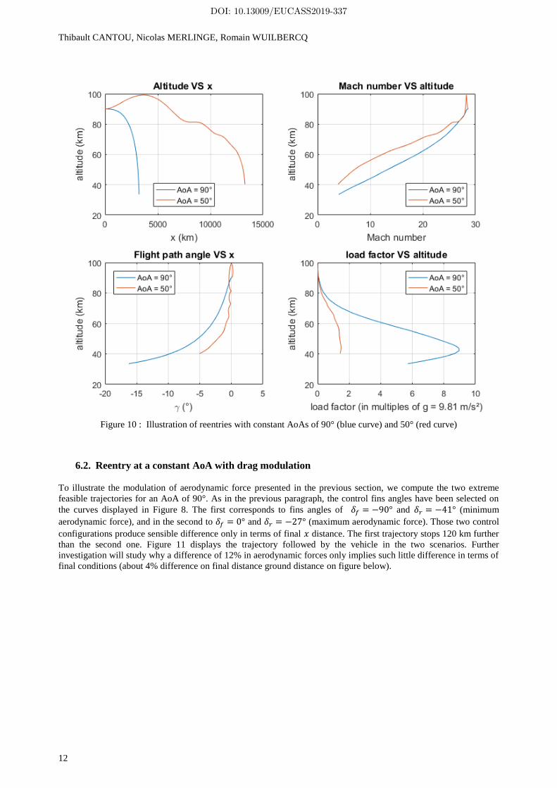
6.1. Reentry with different AoAs

To illustrate the diverse aerodynamic capabilities of the vehicle, we computed the trajectories for two constant AoAs

during reentry. The first case corresponds to an AoA of 90° (negligible lift), and the second one to an AoA 50° (high

lift). The control fins angles have been selected on the curves displayed in Figure 8. Their value is selected on the

corresponding AoA curve at the point corresponding to the middle of the 𝛿𝑓 available domain: in the first case we

choose 𝛿𝑓 = −45° and 𝛿𝑟 = −36°, and in the second case we choose 𝛿𝑓 = −75° and 𝛿𝑟 = −8°. The Figure 10

displays the obtained results for those two simulations.

As it is demonstrated on the Altitude VS 𝑥 plot, the vehicle’s ability to fly with an AoA between 90° and 50° will

allow for very different reentry trajectories. The load factor is drastically lower on the AoA 50° trajectory (about 1.6

g) than on the AoA 90° trajectory (almost 9 g). It is explained by the fact that aerodynamic lift allows the vehicle to

stay longer in the thin high atmosphere which allows it as a consequence to reduce less fast its kinetic energy than in

the case without lift. Manned transportation applications and structure design requirements urge to select a reentry

trajectory with an AoA allowing for lift generation.

Note that these conclusions heavily rely on initial reentry conditions. With the selected set of initial conditions, in the

AoA 50° case, the vehicle generates enough lift force to engage phugoid motion, which is not desirable as we look

for a smooth and steady reentry. Simulations with more representative initial conditions will be part of future studies

to ensure that phugoid motion still happens with an AoA of 50°. An ideal constant AoA would then be found

between 90° and 50° at the lowest AoA without phugoid motion. Future work will also include trajectory

optimization using the AoA as time-dependent control parameter.

DOI: 10.13009/EUCASS2019-337


12

Figure 10 : Illustration of reentries with constant AoAs of 90° (blue curve) and 50° (red curve)

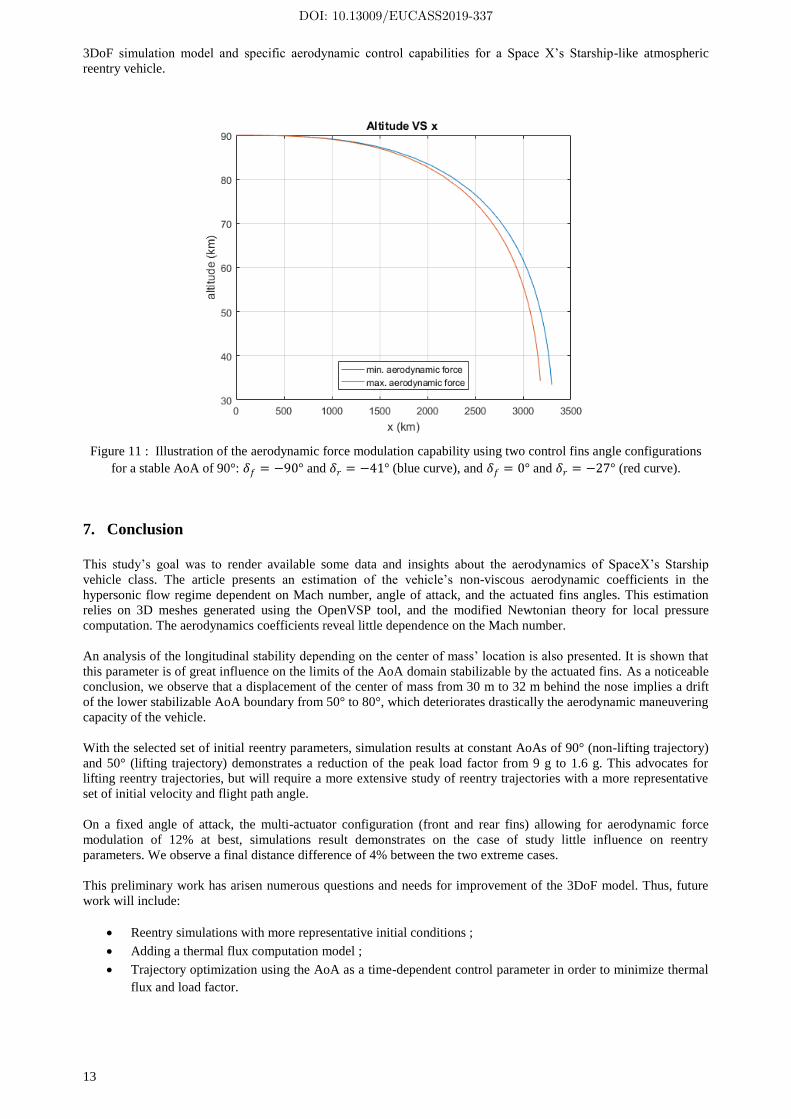
6.2. Reentry at a constant AoA with drag modulation

To illustrate the modulation of aerodynamic force presented in the previous section, we compute the two extreme

feasible trajectories for an AoA of 90°. As in the previous paragraph, the control fins angles have been selected on

the curves displayed in Figure 8. The first corresponds to fins angles of 𝛿𝑓 = −90° and 𝛿𝑟 = −41° (minimum

aerodynamic force), and in the second to 𝛿𝑓 = 0° and 𝛿𝑟 = −27° (maximum aerodynamic force). Those two control

configurations produce sensible difference only in terms of final 𝑥 distance. The first trajectory stops 120 km further

than the second one. Figure 11 displays the trajectory followed by the vehicle in the two scenarios. Further

investigation will study why a difference of 12% in aerodynamic forces only implies such little difference in terms of

final conditions (about 4% difference on final distance ground distance on figure below).

DOI: 10.13009/EUCASS2019-337


reentry vehicle.

13

Figure 11 : Illustration of the aerodynamic force modulation capability using two control fins angle configurations

for a stable AoA of 90°: 𝛿𝑓 = −90° and 𝛿𝑟 = −41° (blue curve), and 𝛿𝑓 = 0° and 𝛿𝑟 = −27° (red curve).

7. Conclusion

This study’s goal was to render available some data and insights about the aerodynamics of SpaceX’s Starship

vehicle class. The article presents an estimation of the vehicle’s non-viscous aerodynamic coefficients in the

hypersonic flow regime dependent on Mach number, angle of attack, and the actuated fins angles. This estimation

relies on 3D meshes generated using the OpenVSP tool, and the modified Newtonian theory for local pressure

computation. The aerodynamics coefficients reveal little dependence on the Mach number.

An analysis of the longitudinal stability depending on the center of mass’ location is also presented. It is shown that

this parameter is of great influence on the limits of the AoA domain stabilizable by the actuated fins. As a noticeable

conclusion, we observe that a displacement of the center of mass from 30 m to 32 m behind the nose implies a drift

of the lower stabilizable AoA boundary from 50° to 80°, which deteriorates drastically the aerodynamic maneuvering

capacity of the vehicle.

With the selected set of initial reentry parameters, simulation results at constant AoAs of 90° (non-lifting trajectory)

and 50° (lifting trajectory) demonstrates a reduction of the peak load factor from 9 g to 1.6 g. This advocates for

lifting reentry trajectories, but will require a more extensive study of reentry trajectories with a more representative

set of initial velocity and flight path angle.

On a fixed angle of attack, the multi-actuator configuration (front and rear fins) allowing for aerodynamic force

modulation of 12% at best, simulations result demonstrates on the case of study little influence on reentry

parameters. We observe a final distance difference of 4% between the two extreme cases.

This preliminary work has arisen numerous questions and needs for improvement of the 3DoF model. Thus, future

work will include:

Reentry simulations with more representative initial conditions ;

Adding a thermal flux computation model ;

Trajectory optimization using the AoA as a time-dependent control parameter in order to minimize thermal

flux and load factor.

DOI: 10.13009/EUCASS2019-337


14

Estimation of the inertia tensor to allow for rotational dynamics simulation and accurate attitude algorithm

design ;

Creation of a more analytic model fitted on the generated database in order to reduce the computational cost

of interpolating the aerodynamic coefficients. Identifying functional dependency of the aerodynamic

coefficients to the flight parameters will allow for easier control studies, particularly in the non-linear

control field.

8. Acknowledgements

We would like to thank Mathieu Balesdent and Loïc Brevault for their constructive remarks that have enriched this

work, and ONERA’s Space Programs Direction to provide us the financial means to attend EUCASS 2019.

References

[1] J. R. Gloudemans, P. C. Davis et P. A. Gehlausen, «A rapid geometry modeler for conceptual aircraft,» chez 34th

Aerospace Sciences Meeting and Exhibit, AIAA, 1996.

[2] Space X, «Making Life Multiplanetary,» [En ligne]. Available: https://www.spacex.com/mars.

[3] J. D. J. Anderson, Hypersonic and High Temperature Gas Dynamics, McGraw-Hill Book Company Series in

Aeronautical and Aerospace Engineering, 1988.

[4] R. Wuilbercq, Multi-disciplinary Modelling of Future Re-usable Space-Access Vehicles, PhD Thesis, University

of Strathclyde, Glasgow, UK, 2015.

[5] L. Lees, «Hypersonic Flow,» chez 5th International Aeronautical Conference, Los Angeles, CA, 1955.

[6] Space X, «Abridged transcript of Elon Musk's presentation - Making Life Multiplanetary,» 2017. [En ligne].

Available: https://www.spacex.com/sites/spacex/files/making_life_multiplanetary_transcript_2017.pdf.

DOI: 10.13009/EUCASS2019-337

yhklfoh - eucass

Documents