yandicoogina 2013 groundwater model setup and calibration

Yandicoogina 2013 Groundwater Model Setup and Calibration of 29

This page is intentional left blank.


Contents page

Introduction 5

1. Introduction 5

Numerical Groundwater Model. 6

2. Numerical Model Code 6

3. Model Setup 6

Model Calibration 17

4. Steady-State Calibration 17

5. Transient calibration 18

6. Assumptions 26

7. Model Limitations 27

8. Summary 27

9. Recommendations 28

References 29

List of Figures

Figure 1 Model Domain and Discretisation..................................................................... 7

Figure 2 Vertical Discretisation – East West Cross-Section along 13984mN. ................. 7

Figure 3 Vertical Discretisation – North South Cross-Section along 21015mE. ............... 8

Figure 4 Hydraulic Parameter Zones – Plan View (Layer 1 and 5). ................................ 9

Figure 5 Hydraulic Parameter Zones – Plan View (Layer 1 and 5). .............................. 10

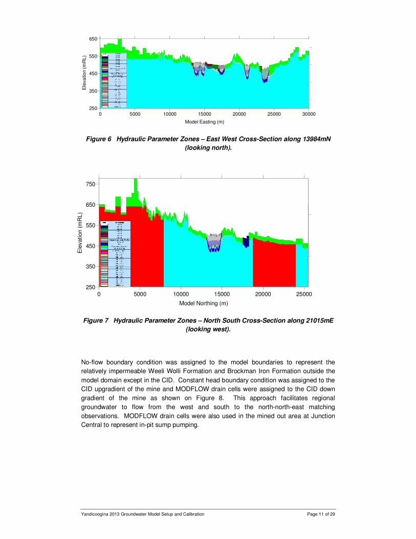
Figure 6 Hydraulic Parameter Zones – East West Cross-Section along 13984mN

(looking north). .............................................................................................................. 11

Figure 7 Hydraulic Parameter Zones – North South Cross-Section along 21015mE

(looking west). ............................................................................................................... 11

Figure 8 Model Boundary Conditions. .......................................................................... 12

Figure 9 Recharge Zones. ........................................................................................... 13

Figure 10 MODFLOW Stream Cells............................................................................. 14

Figure 11 Evapotranspiration Zones. ........................................................................... 15

Figure 12 Dewatering and Injection Bores (1998 to 2013). ........................................... 16


Figure 13 Simulated Steady-State Water Table (mRL)................................................. 18

Figure 14 Location of Calibration bores. ...................................................................... 19

Figure 15 Transient Calibration - Observed versus Calculated Heads. ......................... 20




Figure 19 Transient Calibration Mass Balance. ............................................................ 25

Figure 20 Transient Calibration - Discrepancy Errors. .................................................. 26

List of Tables

Table 1 Recharge Zones and Scaling Factors. ............................................................ 17

Table 2 Evapotranspiration Zones Rates and Extinction Depths. ................................. 17

Table 3 Steady-State Water Balance Summary. .......................................................... 18

Table 4 Hydraulic Parameters of Zones. ...................................................................... 24


Introduction

1. Introduction

Rio Tinto Iron Ore (RTIO) developed a numerical groundwater model in 2008 for

Yandicoogina Operations (Yandi). The model was developed for the 45C licence

application and assessing dewatering requirements for the site. The model domain was

limited to mining and dewatering at Junction Central and Junction South East.

As part of Yandi’s expansion work (below water table mining at Junction South West

(JSW) is to commence in 2014 and Billiards South (BS) is undergoing a pre-feasibility

study) the model domain needed to be extended to minimise boundary effects from

dewatering in the Channel Iron Deposit (CID). Based on the 2008 model, the new model

domain was extended to the west and north and updated with the alluvium layer defined

in the 2010 regional groundwater model (RTIO-PDE-0078850). The number of model

layer was also increased from 7 to 15 to refine the geology from RTIO Vulcan geology

block model for JSW and BS. The model was calibrated against observed hydrographs

from 1998.

This report presents the model setup and calibration of the new model. The intent of the

model is to predict water table level for the medium-term-plan (MTP), assess what if’s

scenarios and set dewatering targets for Operations.


Numerical Groundwater Model.

2. Numerical Model Code The modelling code selected to simulate the groundwater flow condition at Yandicoogina

was MODSURFACT version 3.0. MODSURFACT is an enhanced version of the widely

used United States Geological Survey MODFLOW. MODSURFACT was used mainly to

overcome the numerical instability associated with MODFLOW rewetting of dry cells, and

better representation of dewatering wells with Fractured Well Package. The solver

selected was PCG5 with adaptive time stepping. MODSURFACT was developed by

HydroGeoLogic, Inc. The pre- and post-processor used was Visual MODFLOW version

4.3 developed by Schlumberger Water Services.

3. Model Setup The numerical model domain extends 25.5 km north-south and 30km east-west to cover

the CID areas and minimise model boundary effects (Figure 1).

MODSURFACT is a finite-difference numerical code that requires the model domain to be

discretised into three-dimensional blocks that broadly represent the rock mass within it.

The model setup consists of 425 rows, 491 columns and15 layers. Irregular grids were

used to capture the required hydrogeological details, maintain numerical stability, and

minimise model runtime. The smallest grid measures 31m x 32m and the largest blocks

measures 509m x 750m (Figure 1). The top of layer 1 was assigned the elevations of the

surface topography and the bottom layer is flat at 250mRL. Variable layer thicknesses

were used to capture the geology in the CID as shown on Figures 2 and 3.


0 5000 10000 15000 20000 25000 30000

Model Easting (m)

0

5000

10000

15000

20000

25000

Mo

de

l N

ort

hin

g (

m) Junction Central

Figure 1 Model Domain and Discretisation.

0 5000 10000 15000 20000 25000 30000

Model Easting (m)

250

350

450

550

650

Ele

va

tio

n (

mR

L)

Figure 2 Vertical Discretisation – East West Cross-Section along 13984mN.


0 5000 10000 15000 20000 25000

Model Northing (m)

250

350

450

550

650

750

Ele

vatio

n (

mR

L)

Figure 3 Vertical Discretisation – North South Cross-Section along 21015mE.

The hydrostratigraphic units were based on geo-stratigraphical interpretations consisting

of the alluvial, eastern clay conglomerate (ECC), weathered channel deposit (WCH),

goethite vitreous upper (GVU) and goethite vitreous lower (GVL), limonitic goethite clay

(LGC), basal clay conglomerate (BCC), Weeli Wolli Formation and Brockman Iron

Formation resource drilling database and Vulcan geology block model.

Figures 4 and 5 show the distribution of the hydrostratigraphic units in layers 1, 5, 10 and

15 and Figures 6 and 7 show cross-sectional views. The hydraulic characteristics of

these materials were initially estimated from aquifer test pumping conducted mainly within

the CID and adjusted through calibration to long term pumping. Outside the CID, the

thicknesses of the alluvial and weathered basement were broadly assumed due to limited

available data. As the Weeli Wolli Formation and the Brockman Iron Formation within the

model domain is fractured, these domains were assumed permeable and modelled as

equivalent porous media.


0 5000 10000 15000 20000 25000 30000

Model Easting (m)

0

5000

10000

15000

20000

25000

Mo

de

l N

ort

hin

g (

m)

Layer 5

0 5000 10000 15000 20000 25000 30000

Model Easting (m)

0

5000

10000

15000

20000

25000

Mo

de

l N

ort

hin

g (

m)

Layer 1

Figure 4 Hydraulic Parameter Zones – Plan View (Layer 1 and 5).


0 5000 10000 15000 20000 25000 30000

Model Easting (m)

0

5000

10000

15000

20000

25000

Mod

el N

ort

hin

g (

m)

Layer 15

0 5000 10000 15000 20000 25000 30000

Model Easting (m)

0

5000

10000

15000

20000

25000

Mo

del N

ort

hin

g (

m)

Layer 10

Figure 5 Hydraulic Parameter Zones – Plan View (Layer 1 and 5).


0 5000 10000 15000 20000 25000 30000

Model Easting (m)

250

350

450

550

650

Ele

va

tion (

mR

L)

Figure 6 Hydraulic Parameter Zones – East West Cross-Section along 13984mN

(looking north).

0 5000 10000 15000 20000 25000

Model Northing (m)

250

350

450

550

650

750

Ele

vation (

mR

L)

Figure 7 Hydraulic Parameter Zones – North South Cross-Section along 21015mE

(looking west).

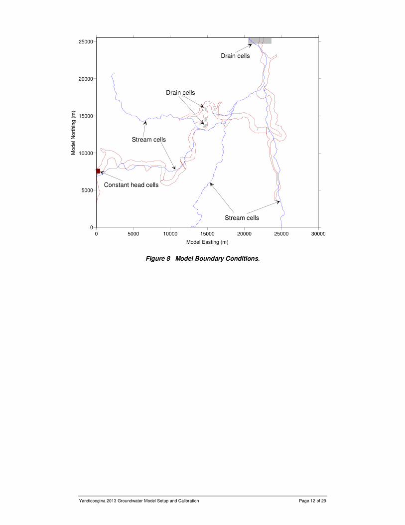
No-flow boundary condition was assigned to the model boundaries to represent the

relatively impermeable Weeli Wolli Formation and Brockman Iron Formation outside the

model domain except in the CID. Constant head boundary condition was assigned to the

CID upgradient of the mine and MODFLOW drain cells were assigned to the CID down

gradient of the mine as shown on Figure 8. This approach facilitates regional

groundwater to flow from the west and south to the north-north-east matching

observations. MODFLOW drain cells were also used in the mined out area at Junction

Central to represent in-pit sump pumping.


0 5000 10000 15000 20000 25000 30000

Model Easting (m)

0

5000

10000

15000

20000

25000

Mo

de

l N

ort

hin

g (

m)

Drain cells

Constant head cells

Stream cells

Drain cells

Stream cells

Figure 8 Model Boundary Conditions.


Direct rainfall recharge is represented in the model by MODFLOW recharge cells with

selection that recharge enters the highest saturated layer i.e. cells that contain the water

table. As direct rainfall recharge to the water table potentially occurs when it rains,

measured rainfall were used to temporally vary monthly recharge rates assigned to the

MODFLOW recharge cells. This simplified approach scaled the monthly measured

rainfall and assumes all infiltration assigned enters the water table. Figure 9 shows the

recharge zones assigned to the model based on surface geology and geomorphology.

Although this approach is not very accurate in an arid environment, it serves as an

approximation of seasonal rainfall recharge.

0 5000 10000 15000 20000 25000 30000

Model Easting (m)

0

5000

10000

15000

20000

25000

Mo

del N

ort

hin

g (

m)

Figure 9 Recharge Zones.

Indirect rainfall recharge from leakage from the creeks was modelled with MODFLOW

stream cells. The use of stream cells accounts for losses and gains along the creek i.e.

leakage upstream results in reduction in stream flow downstream. This is important in

the model because Marillana Creek intersects the CID at a number of places where

leakage potentially occurs. Dewatering in the CID has the potential to induce more

leakage and hence lessen the amount of water that moves downstream and be available

downstream. The rate of leakage is controlled by the streambed conductance of the

stream cells. The variability and lack of measured values of the conductance between

the creeks and the underlying aquifers has resulted in the trial and error adjustment of the

streambed conductance in the model calibration. A uniform rectangular stream width of


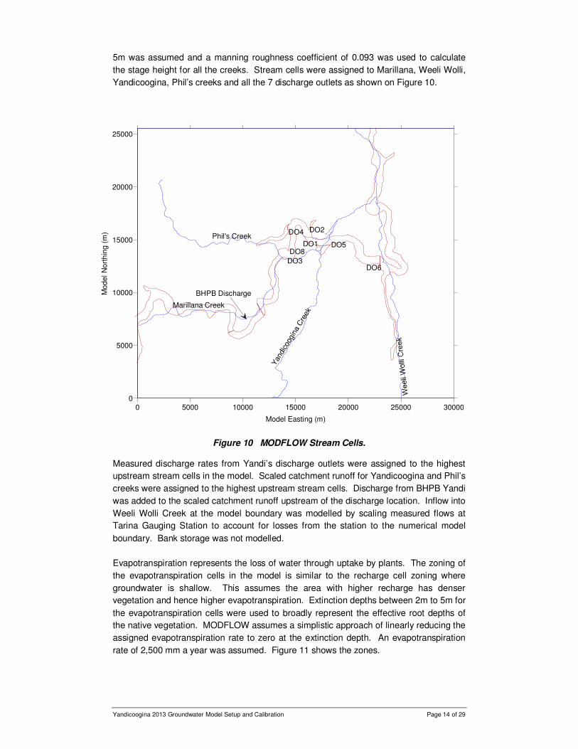
5m was assumed and a manning roughness coefficient of 0.093 was used to calculate

the stage height for all the creeks. Stream cells were assigned to Marillana, Weeli Wolli,

Yandicoogina, Phil’s creeks and all the 7 discharge outlets as shown on Figure 10.

0 5000 10000 15000 20000 25000 30000

Model Easting (m)

0

5000

10000

15000

20000

25000

Mo

de

l N

ort

hin

g (

m) DO4

DO8

DO6

DO5

DO3

DO1

DO2

Marillana Creek

Phil's Creek

BHPB Discharge

Figure 10 MODFLOW Stream Cells.

Measured discharge rates from Yandi’s discharge outlets were assigned to the highest

upstream stream cells in the model. Scaled catchment runoff for Yandicoogina and Phil’s

creeks were assigned to the highest upstream stream cells. Discharge from BHPB Yandi

was added to the scaled catchment runoff upstream of the discharge location. Inflow into

Weeli Wolli Creek at the model boundary was modelled by scaling measured flows at

Tarina Gauging Station to account for losses from the station to the numerical model

boundary. Bank storage was not modelled.

Evapotranspiration represents the loss of water through uptake by plants. The zoning of

the evapotranspiration cells in the model is similar to the recharge cell zoning where

groundwater is shallow. This assumes the area with higher recharge has denser

vegetation and hence higher evapotranspiration. Extinction depths between 2m to 5m for

the evapotranspiration cells were used to broadly represent the effective root depths of

the native vegetation. MODFLOW assumes a simplistic approach of linearly reducing the

assigned evapotranspiration rate to zero at the extinction depth. An evapotranspiration

rate of 2,500 mm a year was assumed. Figure 11 shows the zones.


0 5000 10000 15000 20000 25000 30000

Model Easting (m)

0

5000

10000

15000

20000

25000

Mod

el N

ort

hin

g (

m)

Figure 11 Evapotranspiration Zones.

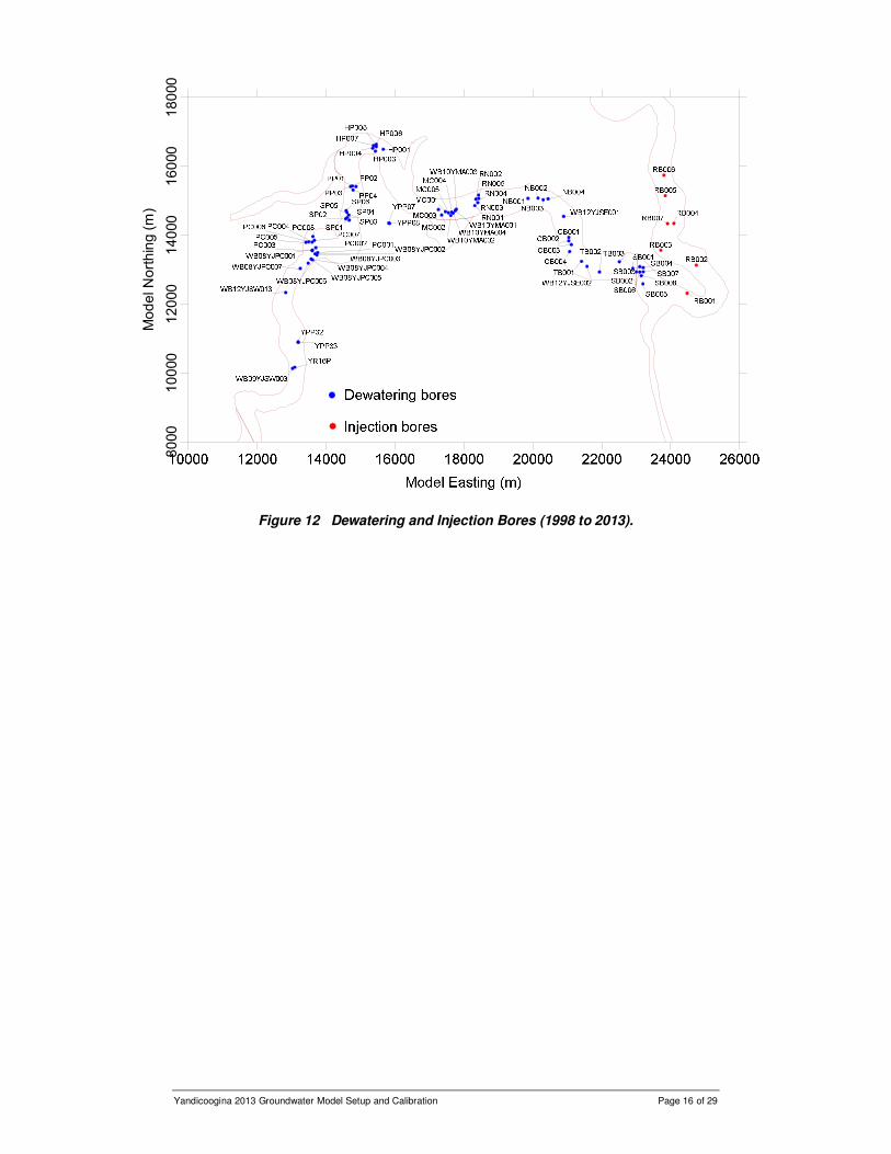
MODSURFACT Fractured Well Package was used to model abstraction and injection

from and to wells. The package treats the screened section as a highly conductive zone,

similar to the behaviour of an actual screen section, in computing inflows into the well

from each aquifers intersected. Measured abstraction and injection rates since 1998

were reduced to monthly rates and assigned to the model. The screened intervals were

simplified to include the GVL and the LGC layers, however, if these layers are thin then

the screened intervals were extended to include the GVU and/or the BCC layers. This

assumes that the LGC, being most permeable, can effectively drain the upper layers.

Figure 12 shows the location of the dewatering and injection bores assigned to the model

since 1998.


8000

10000

12000

14000

16000

18000

Model Northing (m)

Figure 12 Dewatering and Injection Bores (1998 to 2013).


Model Calibration

4. Steady-State Calibration The model steady-state calibration process adopted involved the establishment of a

water level condition consistent with pre-abstraction water level. Groundwater in steady-

state assumes a state of equilibrium where inflows equal outflows i.e. no storage gain or

loss. The dynamic nature of the system to recharge meant that only quasi steady-state

conditions exist. The purpose is to establish an initial/starting water level for the transient

calibration. Water levels measured pre-1998 was used as target for the steady-state

calibration. Hydraulic conductivity and boundary conditions were adjusted in the

calibration process.

Table 1 lists the scaling factors applied to the measured monthly rainfall and Table 2 lists

the extinction depths required to calibrate the model.

Table 1 Recharge Zones and Scaling Factors.

Zone Description Percentage of annual rainfall

1 Weeli Wolli Formation 1%

2 Channel Iron Deposit 7.5%

3 Alluvial 5%

4 Brockman Iron Formation 0.5%

5 Low permeability WW Fm 0%

Table 2 Evapotranspiration Zones Rates and Extinction Depths.

Zone Descriptions Extinction Depth (m)

1 Weeli Wolli Formation/Brockman Iron

Formation/Low permeability WW Fm

2

2 Channel Iron Deposit 3

3 Alluvial 5

Figure 13 shows the simulated steady-state water table and Table 3 lists the mass

balance within the model domain.


490

495

51

0

510

515

525

540

0 5000 10000 15000 20000 25000 30000

Model Easting (m)

0

5000

10000

15000

20000

25000

Mo

del N

ort

hin

g (

m)

Figure 13 Simulated Steady-State Water Table (mRL).

Table 3 Steady-State Water Balance Summary.

Volume In Volume Out

Total (m3/d) % of Total Total (m3/d) % of Total

Stream Leakage 107,319 92 62,729 54

Recharge 1,403 1 0 0

ET 0 0 35,196 30

Constant Head 7663 7 7 0

Drain Cells 0 0 18,425 16

Total 116,385 100 116,350 100

5. Transient calibration Following an acceptable match of the simulated steady-state water table with pre-

abstraction water levels, the steady-state model was converted to the transient model by

activating all transient parameters and boundary conditions. Historical abstraction,

injection and discharge rates, and water levels from observation bores from January 1998

to July 2013 were used in the calibration – a period of 14.5 years.


Monthly stress periods were used to capture the changes in abstraction, injection and

recharge rates. Scaling factors for rainfall recharge and stream flows from the steady-

state calibration were adopted in the transient calibration. Specific yield and specific

storage of each of the hydrostratigraphic units were adjusted, within bounds, in the

transient calibration. Calibration was done by comparing simulated hydrographs with

measured hydrographs. Figure 14 shows the locations of the calibration bores. Both

quantitative (water level matching) and qualitative (trend matching) methods were used to

guide the model calibration. Any changes to hydraulic conductivity and boundary

conditions require recalibration of the steady-state model. Figures 15 to 18 show

simulated versus observed hydrographs in the calibration bores. Observed values are

represented by the green dots and simulated hydrographs by the blue lines.

Figure 14 Location of Calibration bores.


470

475

480

485

490

495

500

505

510

515

520

Wate

r L

evels

(m

AH

D)

Date

MARILLANA1/1(Calculated) Marillana1/1(Observed)

470

475

480

485

490

495

500

505

510

515

520

Wate

r L

eve

l (m

AH

D)

Date

MARILLANA2/1(Calculated) Marillana2/1(Observed)

460

470

480

490

500

510

520

Wate

r L

ev

el (m

AH

D)

Date

YJ-P99/1(Calculated) YJ-P99/1(Observed)

455

460

465

470

475

480

485

490

495

500

505

Wate

r L

ev

el (m

AH

D)

Date

PIEZO4/1(Calculated) Piezo4/1(Observed)

460

465

470

475

480

485

490

495

500

505

510

Wate

r L

ev

el (m

AH

D)

Date

D03YJ1656/1(Calculated) D03YJ1656/1(Observed)

460

465

470

475

480

485

490

495

500

505

510

Wate

r L

evel (m

AH

D)

Date

D03YJ1653/1(Calculated) D03YJ1653/1(Observed)

460

465

470

475

480

485

490

495

500

505

510

Wate

r L

evel (m

AH

D)

Date

YM118/1(Calculated) YM118/1(Observed)

460

465

470

475

480

485

490

495

500

505

510

Wate

r L

eve

l (m

AH

D)

Date

JSEB2/1(Calculated) JSEB2/1(Observed)

410

420

430

440

450

460

470

480

490

500

510

Wate

r L

ev

el (m

AH

D)

Date

JSEB4/1(Calculated) JSEB4/1(Observed)

460

465

470

475

480

485

490

495

500

505

510

Wate

r L

evel (m

AH

D)

Date

JSE25/1(Calculated) JSE25/1(Observed)

Figure 15 Transient Calibration - Observed versus Calculated Heads.


460

465

470

475

480

485

490

495

500

505

510

Wate

r L

ev

el (m

AH

D)

Date


460

465

470

475

480

485

490

495

500

505

510

Wate

r L

ev

el (m

AH

D)

Date


460

465

470

475

480

485

490

495

500

505

510

Wate

r L

eve

l (m

AH

D)

Date

99YJWB02/1(Calculated) 99YJWB02/1(Observed)

460

465

470

475

480

485

490

495

500

505

510

Wa

ter

Lev

el (m

AH

D)

Date


460

465

470

475

480

485

490

495

500

505

510

Wate

r L

evel (m

AH

D)

Date


460

465

470

475

480

485

490

495

500

505

510

Wate

r L

evel (m

AH

D)

Date


460

465

470

475

480

485

490

495

500

505

510

Wate

r L

evel (m

AH

D)

Date


460

465

470

475

480

485

490

495

500

505

510

Wate

r L

ev

el (m

AH

D)

Date

WW2/1(Calculated) WW2/1(Observed)

460

465

470

475

480

485

490

495

500

505

510

Wate

r L

evel (m

AH

D)

Date


460

465

470

475

480

485

490

495

500

505

510

Wate

r L

evel (m

AH

D)

Date




460

465

470

475

480

485

490

495

500

505

510

Wa

ter

Level

(mA

HD

)

Date


460

465

470

475

480

485

490

495

500

505

510

Wate

r L

evel (m

AH

D)

Date


460

465

470

475

480

485

490

495

500

505

510

Wa

ter

Level

(mA

HD

)

Date


460

465

470

475

480

485

490

495

500

505

510

Wate

r L

evel (m

AH

D)

Date


460

465

470

475

480

485

490

495

500

505

510

Wate

r L

evel (m

AH

D)

Date


460

465

470

475

480

485

490

495

500

505

510

Wate

r L

evel (m

AH

D)

Date


460

465

470

475

480

485

490

495

500

505

510

Wate

r L

evel (m

AH

D)

Date


460

465

470

475

480

485

490

495

500

505

510

Wate

r L

evel (m

AH

D)

Date


460

465

470

475

480

485

490

495

500

505

510

Wate

r L

ev

el (m

AH

D)

Date


460

465

470

475

480

485

490

495

500

505

510

Wate

r L

evel (m

AH

D)

Date




460

465

470

475

480

485

490

495

500

505

510

Wate

r L

ev

el (m

AH

D)

Date

YM119/1(Calculated) YM119/1(Observed)

460

465

470

475

480

485

490

495

500

505

510

Wate

r L

ev

el (m

AH

D)

Date

UN34/A(Calculated) UN34

460

465

470

475

480

485

490

495

500

505

510

Wate

r L

ev

el (m

AH

D)

Date

D04YJ2026 D04YJ2026

460

465

470

475

480

485

490

495

500

505

510

Wate

r L

evel (m

AH

D)

Date

D08YJ126 D08YJ126

460

465

470

475

480

485

490

495

500

505

510

Wa

ter

Le

vel (m

AH

D)

Date

99YJWB04/1(Calculated) 99YJWB04/1(Observed)

480

485

490

495

500

505

510

515

520

525

530

Wate

r L

ev

el (m

AH

D)

Date

PZ08YJSW001 PZ08YJSW001

480

485

490

495

500

505

510

515

520

525

530

Wate

r L

evel (m

AH

D)

Date


480

485

490

495

500

505

510

515

520

525

530

Wa

ter

Le

vel (m

AH

D)

Date


480

485

490

495

500

505

510

515

520

525

530

Wate

r L

ev

el (m

AH

D)

Date




Table 4 lists the hydraulic parameters derived from the model calibration

(F3D_TrCal14ext_2013d.vmf). The hydraulic parameters were generally similar to the

previous model.

Table 4 Hydraulic Parameters of Zones.

Water balance from the transient calibration indicates that increased dewatering at Yandi

increased leakage from the creeks and evapotranspiration was slightly higher possibly

due to the increased water in the creeks as shown in Figure 19.


Figure 19 Transient Calibration Mass Balance.

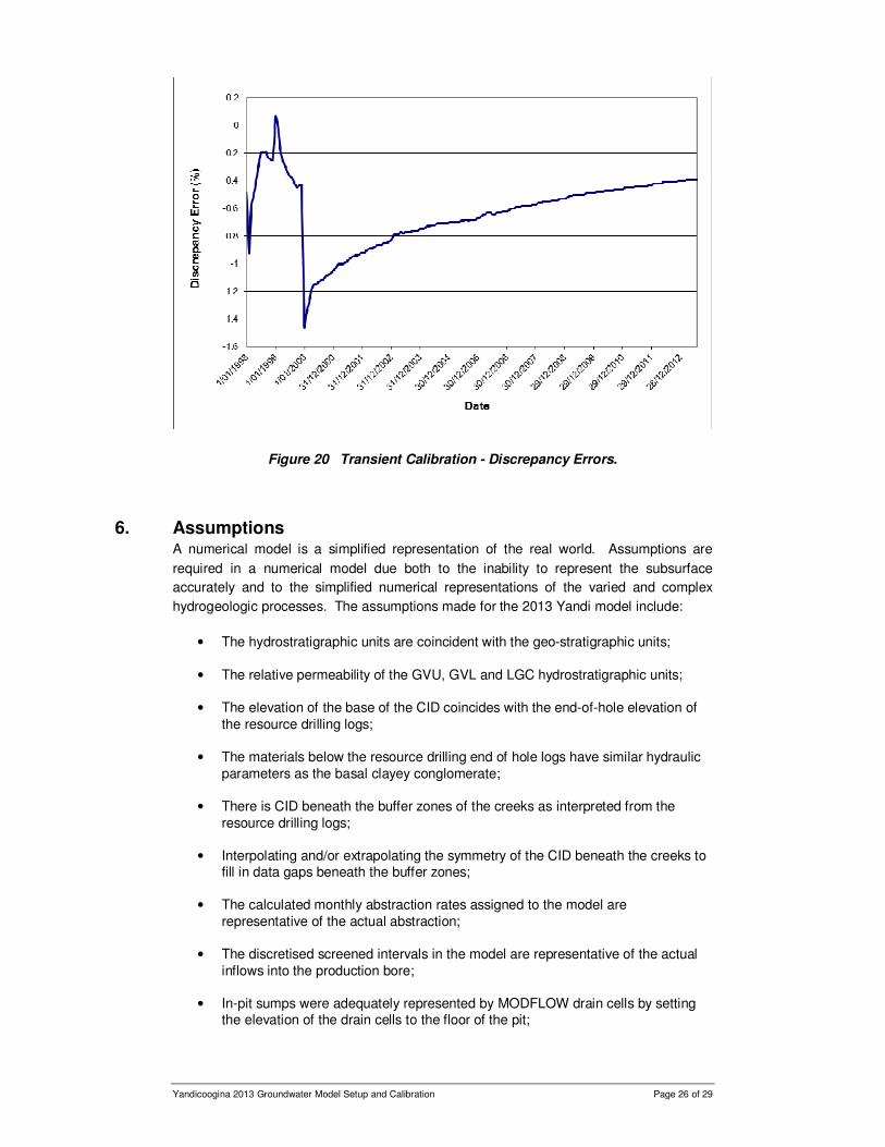
Figure 20 shows the percentage discrepancy errors from the transient model calibration

simulation. Percentage discrepancy error below 5% is considered good for complex flow

systems.


Figure 20 Transient Calibration - Discrepancy Errors.

6. Assumptions A numerical model is a simplified representation of the real world. Assumptions are

required in a numerical model due both to the inability to represent the subsurface

accurately and to the simplified numerical representations of the varied and complex

hydrogeologic processes. The assumptions made for the 2013 Yandi model include:

• The hydrostratigraphic units are coincident with the geo-stratigraphic units;

• The relative permeability of the GVU, GVL and LGC hydrostratigraphic units;

• The elevation of the base of the CID coincides with the end-of-hole elevation of

the resource drilling logs;

• The materials below the resource drilling end of hole logs have similar hydraulic

parameters as the basal clayey conglomerate;

• There is CID beneath the buffer zones of the creeks as interpreted from the

resource drilling logs;

• Interpolating and/or extrapolating the symmetry of the CID beneath the creeks to fill in data gaps beneath the buffer zones;

• The calculated monthly abstraction rates assigned to the model are

representative of the actual abstraction;

• The discretised screened intervals in the model are representative of the actual

inflows into the production bore;

• In-pit sumps were adequately represented by MODFLOW drain cells by setting the elevation of the drain cells to the floor of the pit;


• The amount of water discharged into the WFC was completely recovered by the

in-pit sumps or evaporated;

• The width of the creeks was fixed at 5.0m and a manning roughness coefficient

of 0.093 accounts for the increased river stage when flows in the creeks increased;

• The slopes and elevations of the creeks can be computed from the topographical

data;

• Conductances for the creek beds derived from model calibration are an accurate

representation of the conductance between the creeks and the underlying water table aquifers;

• Scaling of monthly rainfall to represent infiltration to the water table is

representative of the total rainfall recharge to the aquifers;

• The recharge zones used in the model can adequately account for the total

recharge to the aquifers;

• Scaling of monthly rainfall in catchment upstream of BHPB discharge point is a good approximation of the flow in Marillana Creek upstream of the discharge point;

• Scaling of monthly rainfall in catchment upstream of Phil’s and Yandicoogina

creeks are good approximation of the flow in these creeks;

• Bank storage can be ignored;

• The evapotranspiration zones and extinction depths used in the model

adequately account for the total loss of groundwater to the atmosphere;

• Recent interpretation of the pinching out of the Weeli Wolli Formation north, the

CID and alluvium directly overlies the BIF and a large mineralised BIF occurs

underneath the outwash has insignificant impacts on the model prediction.; and

• The higher in flows from the constant head boundaries along Marillana Creek

provides a conservative approach to dewatering.

7. Model Limitations According to the 2012 Australian Groundwater Modelling Guidelines confidence level

classification, the Yandi numerical groundwater model can be classed as Class 3 model

for 5 year model prediction. Longer term model prediction would lower the confidence

level classification.

8. Summary The Yandi 2008 numerical groundwater model domain was limited to mining and

dewatering at Junction Central and Junction South East. As part of Yandi’s expansion

work to include Junction South West and Billiards South, the model domain was

extended to minimise boundary effects from dewatering in these areas in the Channel

Iron Deposit. The rebuild/update of the model included the alluvium layer defined in the


2010 regional groundwater model (RTIO-PDE-0078850). The number of model layer

was increased from 7 to 15 to refine the geology from RTIO Vulcan geology block model.

The model was calibrated in steady-state and transient with abstraction, injection and

discharge rates, and water levels from observation bores from January 1998 to July

2013. Both calibrations show the model is representative of the site and according to the

2012 Australian Groundwater Modelling Guidelines confidence level classification, the

model can be classed as Class 3 for model prediction up to 5 years.

9. Recommendations It is recommended that the model be:

• recalibrated at least once a year to maintain currency of the model; and

• refinement in the Oxbow and Billiards North areas for future model calibration.


References

Australian Government National Water Commission (2012), Australian groundwater

modelling guidelines, Waterlines Report series No. 82.

yandicoogina 2013 groundwater model setup and calibration

Documents