AdaptiveExtremum

Control

and

W

indTurbineControl

XinMa

May1997

Copyrightc 1997byXinMa

Preface

Thisthesisissubmittedinpartialful�llmentoftherequirementsforthedegree

ofPh.D.inengineering.ThethesishasbeenpreparedattheInstituteofMathe-

maticalModelling(IMM),theTechnicalUniversityofDenmark(DTU).

Thisthesisconsistsoftwoparts,i.e.,adaptiveextremum

controlandmodelling

andcontrolofawindturbine.

The�rstpartofthethesisdiscussesdesignofadaptiveextremumcontrollersfor

someprocesseswhichhavethebehaviourthattheprocessshouldhaveashigh

e�ciencyaspossible.Themaincontributionisthedevelopmentofanadaptive

extremumcontrolalgorithmbasedontheparameterestimationfortheprocesses

withoutputnonlinearity.

Thesecondpartofthethesisisconcernedwithmodellingandcontrolofawind

turbine.Theinvestigationofcontroldesignisdividedintobelowratedoperation

andaboveratedoperation.

Thebehaviourofwindturbinesinbelowratedoperationbelongstotheprocess

discussedinthe�rstpartofthethesis,whichcanbeconsideredasaconnection

betweentwoparts.

i

ii

Acknowledgements

Itispleasureformetaketheopportunitytoexpressmygratefulnessto

everybodywhoenabledmetoperformtheworkpresentedinthisthesis.

First,IwishtoexpressmythankstomysupervisorNielsKj�stadPoulsen

(IMM)andHenrikBindner(Ris�NationalLaboratory)fortheirwillingto

bemysupervisorsandtheirinterestsintheproject.Further,Ithankthem

forreadingthe�rstversionofthethesisandforgivinghelpfulcomments.

Iwouldalsoliketothankthesta�attheIMM,myfriendsAncaDaniella

Hansenforenjoyabledailycompany,andLarsHenrikHansenwhohasal-

waystimeandpatiencewithmyquestions.EspeciallyIwishtothankthe

librarianFinnKunoChristensenforhishelpto�ndliteraturesources.

Igreatlyappreciatethesupportbymyparentsandmyparents-in-law,who

havehelpedmetotakecareofmysonduringmystudy.Iwouldalsolike

tothankmysonJohanZiruoYeforhisunderstanding.

iii

iv Finally,AspecialacknowledgeistomyhusbandTaoYe,whomIcannever

thankenoughforhissupportandencouragement.

Lyngby,Denmark,May1997.

XinMa

Summary

Thisthesisisdividedintotwoparts,i.e.,adaptiveextremumcontroland

modellingandcontrolofawindturbine.

The�rstpartofthethesisdealswiththedesignofadaptiveextremum

controllersforsomeprocesseswhichhavethebehaviourthatprocessshould

haveashighe�ciencyaspossible.

Firstly,itisassumedthatthenonlinearprocessescanbedividedintoa

dynamiclinearpartandstaticnonlinearpart.Consequentlytheprocesses

withinputnonlinearityandoutputnonlinearityaretreatedseparately.

Withthenonlinearityattheinputitiseasytosetupamodelwhichis

linearinparameters,andthusdirectlylendsitselftoparameterestimation

andadaptivecontrol.Theextremumcontrollawisderivedbasedonstatic

optimizationofaperformancefunction.

Foraprocesswithnonlinearityatoutputtheintermediatesignalbetween

thelinearpartandnonlinearpartplaysanimportantrole.Ifitcanbe

v

vi

known,theonlydi�erencebetweentheoutputnonlinearityandinputnon-

linearityisthatitsextremumcontrollawwillbedeterminedthroughlinear

dynamics.Iftheintermediatesignalisnotavailable,theemphasiswill

belaidontheparameterestimationapproaches.TheEKFandRPEM

methodsaredevelopedforstateandparameterestimationforanonlinear

system.

Thesecondpartofthethesisdiscussestheaspectsonmodellingandcontrol

ofawindturbine.

Specialattentionispaidtomathematicalmodellingofwindturbineswith

emphasisoncontroldesign.Themodelshavebeenvalidatedbyexperimen-

taldataobtainedfromanexistingwindturbine.

Thee�ectivewindspeedexperiencedbytherotorofawindturbine,which

isoftenrequiredbysomecontrolmethods,isestimatedbyusingawind

turbineasawindmeasuringdevice.

Theinvestigationofcontroldesignisdividedintobelowratedoperationand

aboveratedoperation.Belowratedpower,theaimofcontrolistoextract

maximumenergyfromthewind.Thepitchangleoftherotorbladesis�xed

atitsoptimalvalueandturbinespeedisadjustedtofollowthechangesin

windspeed.Aboveratedpower,thecontroldesignproblemistolimitand

smooththeoutputelectricalpower.Thepitchcontrolisinvestigatedfor

bothconstantspeedandvariablespeedwindturbines.Theminimization

oftheturbinetransientloadsisfocussedinbothcases.

Resum�e(inDanish)

N�rv�rendeafhandlingomhandlertorelateredeemner,adaptiveekstremum-

s�geresamtmodelleringogstyringafvindm�ller.

Afhandlingensf�rstedelvedr�reradaptiveekstremums�gere.M�aleterat

introducereenstyringsstrategi,der�geretsystemse�ektivitet.

F�rstantagesdetatdenuline�reprocesbest�arafenline�rdynamiskdel

samtenuline�rstatiskdel.Processermedulineariteteriudgangenogi

indgangenharderesspeci�kkeegenskaber.

Hvisulineariteterneerrelaterettiludgangenkansystemetletbeskrivesaf

enmodeldererline�riparametreneogf�lgeligletindg�aienparameter-

estimationogadaptivregulering.Denekstremums�gendestyrestrategier

udledtudfrastatiskeoptimeringsmetoder.

Hvisulinearitetenerrelaterettilindgangenafsystemetspillerdetpartielle

signalmellemline�roguline�rdelenbestydeligrolle.Erdettesignalkendt

ellerm�altbest�ardenekstremums�gendestyrestrategiafenoptimeringvia

vii

viii

denline�redynamik.Erdettesignalikketilg�ngeligtm�aenestimations-

baseretmetodeanvendes.EnEKFogenRPEM

metodeerudvikletfor

tilstandsogparameterestimation.

Afhandlingensandendelvedr�rermodelleringogstyringafvindm�ller.

Imodelleringenerderfokuseretp�aanvendelsenafmodellentilregulator

design.Modellenerblevetvalideretmodeksperimentelledata.

Dene�ektivevindhastighederenmodelleringstekniskst�rrelse,someret

udtrykforvindensp�avirkningafvindm�llenoganvendesofteifremkoblings-

delenforenstyring.Dereriafhandlingenbeskrevetogdiskuteretmetoder

tilestimationafdene�ektivevindhastighedmedvindm�llensomegentligt

m�alesystem.

Styringafenvindm�llebest�araftoopgaver.Undernominelvindhastighed

erm�aletatoptimeredene�ektderudnyttesfravinden.Vindm�llensblad-

vinkelerfastl�astveddenoptimaleudnyttelsesgradogoml�bstalletjusteres

tilatf�lgevariationerneivindhastigheden.Overnominelvindhastighed

erm�aletatbegr�nsedenoptagnee�ekttilenpr�speci�ceretst�rrelse.

Iafhandlingenbehandlesbladvinkelreguleringmedb�adekonstantogvari-

abeltoml�bstal.

ix

Partsofthisthesishavepreviouslybeenpublishedin

�XinMa.ModellingandControlofaWindTurbine.Master'sthesis,

No.25/93,IMSOR,DTU.

�XinMa,NielsK.PoulsenandHenrikBindner.ModellingandControl

ofaWindTurbine.Technicalreport,IMM-rep-1994-27,IMM,DTU.

�XinMa,NielsK.PoulsenandHenrikBindner.EstimationofWind

SpeedinConnectiontoaWindTurbine.Technicalreport,IMM-rep-

1995-26,IMM,DTU.

�XinMa,NielsK.PoulsenandHenrikBindner.APitchRegulated

VariableSpeedWindTurbine.Technicalreport,IMM-rep-1995-27,

IMM,DTU.

�XinMaandNielsK.Poulsen.AdaptiveExtremumControl.Technical

report,IMM-rep-1996-23,IMM,DTU.

�XinMa,NielsK.PoulsenandHenrikBindner.EstimationofWind

SpeedinConnectiontoaWindTurbine.AcceptedbytheIASTED

InternationalConferenceonControl,Mexico,May,1997.

�XinMa,NielsK.PoulsenandHenrikBindner.ExtremumTracking

ControlofaWindTurbine.Technicalreport,toappear,IMM,DTU.

x

Contents

Preface

i

Acknowledgements

iii

Summary

v

Resum�e(inDanish)

vii

I

AdaptiveExtremum

Control

1

Glossary

3

1

Introduction

5

xi

xii

CONTENTS

2

ModelsofNonlinearDynamicProcesses

17

2.1

Modelsininput-outputformulae................19

2.1.1

Nonlinearityatinput...................19

2.1.2

Nonlinearityatoutput..................21

2.1.3

Somegeneralnonlinearmodels.............22

2.2

Modelsinstate-spaceformulae.................24

2.2.1

Nonlinearityatinput...................24

2.2.2

Nonlinearityatoutput..................25

2.2.3

Ageneralnonlinearstate-spacemodel.........26

2.3

Summary.............................27

3

InputNonlinearity

29

3.1

AdaptiveextremumcontrolforHammersteinmodel.....31

3.1.1

Themodi�edHammersteinmodel...........31

3.1.2

Extremumcontrollaw..................32

3.1.3

Parameterestimation

..................34

CONTENTS

xiii

3.1.4

Theadaptiveextremumcontrolalgorithm

.......35

3.2

Casestudies............................39

3.3

Convergenceanalysis.......................44

3.4

Summary.............................47

4

OutputNonlinearity

49

4.1

Basicextremumcontrollaw...................50

4.2

Theintermediatesignalismeasurable.............52

4.3

Theintermediatesignalisnotmeasurable...........59

4.3.1

TheEKFasaparameterestimatorforthenonlinear

system...........................60

4.3.2

TheRPEMappliedtotheinnovationsmodel.....69

4.3.3

Themodi�edrecursivepredictionerrormethod....76

4.4

Summary.............................82

5

Conclusions

85

Bibliography

89

xiv

CONTENTS

II

ModellingandControlofA

WindTurbine

95

Glossary

97

6

Introduction

101

6.1

Awindturbine..........................102

6.2

Theturbinecontrolproblem...................103

6.3

Outlineofthesecondpartofthethesis.............107

7

SimulationModeloftheWindTurbine

109

7.1

Introduction............................109

7.2

Windmodel............................111

7.2.1

Thepointwindspeed

..................112

7.2.2

Thewindexperiencedbytherotor...........115

7.2.3

Theapproximatede�ectivewindspeed

........115

7.3

Aerodynamics...........................120

7.3.1

Aerodynamicpowerandtorque.............122

CONTENTS

xv

7.3.2

3pe�ect..........................124

7.3.3

Axialforce

........................125

7.4

Structuraldynamics.......................126

7.5

Drivetrain

............................128

7.6

Generatormodel.........................130

7.6.1

Constantspeedpowergenerationunit.........131

7.6.2

Variablespeedpowergeneratorunit..........134

7.7

Pitchactuator

..........................135

7.8

Anentiremodel..........................137

7.9

Validationofmodel........................137

7.9.1

ValidationofT3P

model.................139

7.9.2

Validationresults.....................140

7.9.3

Anotherexperiment...................142

7.10Simulationoftheuncontrolledwindturbine..........143

7.11Summary.............................145

xvi

CONTENTS

8

DesignModeloftheWindTurbine

147

8.1

Linearstate-spacemodelsoftheplant.............149

8.1.1

Aerodynamictorque...................149

8.1.2

Drivetrainandgenerator................150

8.1.3

Abovetheratedwindspeed...............150

8.1.4

Belowtheratedwindspeed...............155

8.2

Noisemodels...........................157

8.3

Acompositemodel........................158

8.4

Discretetimemodel.......................159

8.5

Summary.............................161

9

EstimationofTheWindSpeed

163

9.1

TheNewton-Raphsonmethod..................165

9.2

TheKalman�ltermethod....................169

9.3

TheextendedKalman�ltermethod

..............172

9.3.1

Aboveratedwindspeed.................173

CONTENTS

xvii

9.3.2

Belowratedwindspeed

.................177

9.4

Acomparison...........................179

9.5

Test................................181

9.6

Discussion.............................184

9.7

Summary.............................186

10ControlAboveRatedPower

187

10.1PIpitchcontrol..........................190

10.2LQGpitchcontrol........................195

10.3Combinedvariablespeedandpitchcontrol

..........202

10.4Summary.............................207

11ControlBelowRatedPower

211

11.1LQGspeedcontrol........................214

11.2Trackingcontrol.........................221

11.3Implementationofcontrolsystem

................227

11.4Summary.............................230

xviii

CONTENTS

12SummaryandConclusions

233

Bibliography

241

A

OptimizationBackground

243

A.1

Searchingforanextremum

...................244

A.2

Hill-climbingalgorithm......................246

A.3

Gradientmethod.........................248

A.4

TheNewtonmethod.......................250

A.5

Gauss-Newtonmethod......................253

A.6

Linesearchtechnique

......................254

A.7

Summary.............................258

B

ConvergenceAnalysisforRecursiveAlgorithms

261

B.1

BasicideasofODEapproach

..................262

B.2

GeneralresultsofODE

.....................266

B.3

Localconvergenceofrecursiveleastsquarealgorithm.....268

CONTENTS

xix

C

TheEKFasaJointstateandParameterEstimator

271

C.1

ExtendedKalman�lter

.....................272

C.2

Thesystem

............................273

C.3

Themodel.............................274

C.4

Jointparameterandstateestimation..............274

C.5

Convergenceanalysis.......................280

D

TheRPEMethodAppliedtotheInnovationsModel

285

D.1Themodel.............................285

D.2Thealgorithm...........................286

E

TekniskeDataforWD34WindTurbine

291

PartI

AdaptiveExtremum

Control

1

3

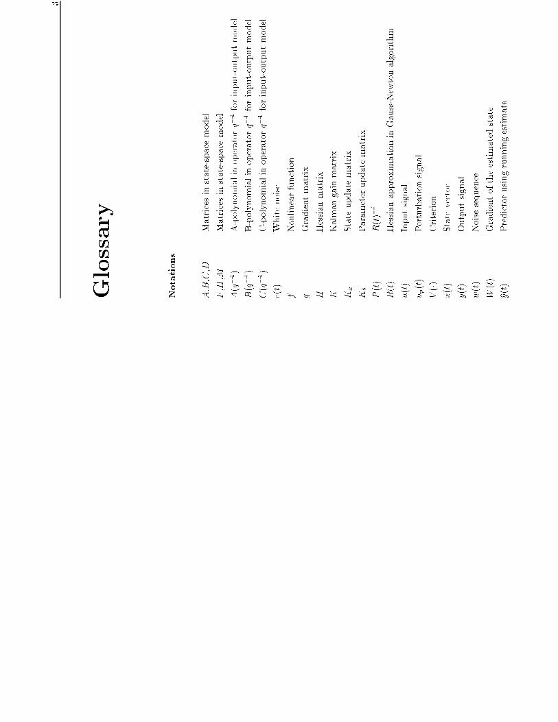
Glossary

Notations

A,B,C,D

Matricesinstate-spacemodel

F,H,M

Matricesinstate-spacemodel

A(q�1)

A-polynomialinoperatorq�1forinput-outputmodel

B(q�1)

B-polynomialinoperatorq�1forinput-outputmodel

C(q�1)

C-polynomialinoperatorq�1forinput-outputmodel

e(t)

Whitenoise

f

Nonlinearfunction

g

Gradientmatrix

H

Hessianmatrix

K

Kalmangainmatrix

Kx

Stateupdatematrix

K�

Parameterupdatematrix

P(t)

R(t)�1

R(t)

HessianapproximationinGauss-Newtonalgorithm

u(t)

Inputsignal

up(t)

Perturbationsignal

V(�)

Criterion

x(t)

Statevector

y(t)

Outputsignal

w(t)

Noisesequence

W(t)

Gradientoftheestimatedstate

^y(t)

Predictorusingrunningestimate

4 z(t)

Intermediatesignal

�(t)

Predictionerror

�

Parametervector

^ �(t)

Recursiveestimateof�

� 0

Truevalueof�

��

Convergentpointof�

'(t)

Vectorformedfromobserveddata

�(t)

Gradientofthepredictionerror

�

Stepsize

�

Covariancematrixofpredictionerror

^ �(t)

Estimatedcovariancematrixofpredictionerror

�

Incrementoperator

Abbreviations

EKF

ExtendedKalmanFilter

LHP

LeftHalfPlane

ODE

OrdinaryDi�erentialEquation

PRBS

PseudorandomBinarySequence

RELS

RecursiveExtendedLeastSquares

RLS

RecursiveLeastSquares

RML

RecursiveMaximumLikelihood

RPEM

RecursivePredictionErrorMethod

Chapter1

Introduction

Inmostcontrolproblems,thetaskofaregulatoristokeepsomevariables

atconstantvalues,ortomakethemfollowreferencesignals.Ingeneral,the

systemisassumedtobelinear,anditispossible,inprinciple,todrivethe

outputtoanyprescribedvalue.Withsuchproblemsthereferencevalues

areofteneasilydetermined.Itcanbethedesiredaltitudeofanairplane,

theprede�nedconcentrationofaproduct.Inthesecasesthecontrolaction

istooptimizeacostfunctionbyinvolvinganestimatedsystemmodel.

Onotheroccasions,itcanbemoredi�cultto�ndthesuitablereference

valuesorthebestoperatingpointsofaprocess.Anumberofindustrial

processeshavethebehaviourthattheprocessshouldhaveashighe�ciency

aspossible,theirperformancecanbeimprovedbyadjustingplantvari-

ablessoastomaximizeorminimizetheperformancecriterion.Totracka

5

6

Chapter1.Introduction

varyingmaximumorminimumiscalledextremumcontrol.Therearesev-

eralexamplesofpracticalsystemsthatexhibitthistypeofbehaviour,e.g.,

powergenerationsystem,chemicalandcombustionprocesses.Oneappli-

cationisspark-ignitionautomotiveengine.Thefuelconsumptionofacar

depends,amongotherthings,ontheignitionangle.Thetaskofadaptive

extremumcontrolistoadjustsparkignitionangleandoperatetheengineat

apredeterminedoptimumvalue.Anotherexampleisore-grinding,where

thegrindinge�ciencywillvarywiththe�llingdegreeofthemill,which

canbecontrolledthroughtheincoming owofrawmaterial.Theoptimal

pointinmaximizinge�ciencymaydependonthequalityandcomposition

ofthisrawmaterial.Forawindturbine,thepitchangleofbladesorthe

rotorspeedofwindturbineischangeddependingonthewindspeedtogive

maximumoutputpower.Thisisalsoanextremumcontrolproblem.

Extremumcontrolsystemshaveonemajorcharacteristicincommon.In

theabsenceofdisturbance,thestaticresponsecurverelatingtheoutputs

toinputsisnonlinearandhasatleastoneextremum.Theobjectiveof

extremumcontrolistokeeptheprocessoperatingat,orinthevicinityof,

theextremumpointoftheperformancefunctionorprocessoutputdespite

changesintheprocessorin uenceofdisturbances.

Acommonassumptionisthatthereisnondynamicsinthesystem.Thisis

calledstaticsystem.Inpractice,thisconditioncanbeful�lledbyusinga

su�cientlylargesamplinginterval.Buttheresultmaybeaslowoptimiza-

tion.Inmanycases,however,staticmodelsmaybeadequate,andstochastic

approximationmethodscanthenbeusedforoptimizationtohandlenoise

measurements.

7

Actuallymorecommoncasesinpracticearetheinputsignalwillin uence

thesystem

behaviouratsubsequenttimes,i.e.,theperformancehasnot

settledatnewsteady-statevaluebeforethenextmeasurementistaken.

Thisissocalleddynamicsystem.Oneofmethodstohandlethiskindof

systemistoderiveanonlineardynamicmodel.

[Blackman1962]isagoodintroductiontothe�eldofextremumcontrol.

Theclassi�cationusedinthispaperisperturbationsystems,switchingsys-

temsandselfdrivingsystems.Intheperturbationsystems,thee�ectat

outputfromaknownsignaladdedtotheinputisusedtoderiveinforma-

tionabouttheslopeofthenonlinearity.Theinformationisthenusedto

drivethesystem

andkeeptheslopeasclosetozeroaspossible.Inaso

calledswitchingsystem,theinputisdrivenbyaconstantspeed ip- opwith

twostates.Iftheextremumispassed,thedirectionofinputdriftisthen

reversedaccordingtosome�xedrules.Thesystemcanthenbeoperatedin

theneighbourhoodoftheextremum.Theselfdrivingsystemsusemeasure-

mentsofthetimederivativeoftheoutputtodeterminetheinput.Ifthe

processisstartedinthecorrectdirection,itwillcontinueuntilextremum

isreached.

Afourthclassofmethodsthatisnotdescribedin[Blackman1962]hasbeen

developedlateron.Itisbasedonusingaparameterizedmodelincombining

parameteridenti�cationandextremumcontrol.Theprojectpresentedhere

isbasedonthistypeofmethods.

Sincefewerideasforextremumcontrolhaveemergedsince60's.Itisthen

stillworthmentioningthethreetypesofmethodsclassi�edby[Blackman196

Themethodswerelatersummarizedby[Sternby80b].

8 Chapter 1. Introduction

Perturbation methods

The basic idea of perturbation methods is to add a periodic test signal to

the control signal, and observe its e�ect at the output. The task of an

extremum controller in the perturbation methods is to keep the gradient of

the nonlinearity at zero.

Input

Output

Figure 1.1. E�ect of input test signal at the output for a static nonlinearity.

The e�ect of an input test signal at output of a static nonlinearity is illus-

trated in Figure 1.1. The most commonly used test signal form is sinusoid.

However, if the system contains dynamics, the dynamics will then introduce

a phase lag � in the test signal component of the output. The result of

correlation will be multiplied by a factor cos �. This gives a sign error

in the correlation signal if � > 900. This situation can be avoided if a

corresponding phase lag is introduced to the test signal before correlation.

Another way is to use a perturbation signal of su�ciently low frequency.

The phase lag will then be small, so that the dynamics can be neglected.

But this give a long response time for the overall system.

With the perturbation signal technique, the correlating device must be given

a certain amount of time to produce an accurate slope signal. During this

9

time the control signal should be kept constant, so that the total input

varies with test signal only.

The perturbation methods may be the oldest extremum control method.

But it is also well suited to multi-input systems. In order to apply a gradient

method in search for an extremum, the partial derivatives of the static

response curve with respect to the di�erent inputs are needed. This can

be realized by using perturbation signals with di�erent frequencies for each

input.

Switching methods

Another basic idea for extremum control is the switching methods. The

input is driven at constant speed in the same direction until no further

improvement is registered. The drift direction is then reversed. Di�erent

algorithms of this type can be described in terms of their speci�c conditions

for altering the direction of input changes. The control law is thus a set of

switching conditions. The input may be changed continuously or in discrete

steps. The second one is called stepping method.

In a continuous sweep method, the sweep direction is reversed when the

output has decreased from its maximum value by a �xed amount �. The

design parameters are then the sweep rate and the value of �. If the output

is disturbed by noise, the method may give excessive switching unless the

value of � is su�ciently increased. But it will on the other hand increase the

hunting loss by increasing �. It is then necessary to compromise in choosing

�. Filtering is another possibility for reducing the noise sensitivity. The

problem is then that more dynamics are introduced into the system, and

the hunting loss will again be increased. Unnecessary switching may also

be caused by input dynamics. The switching conditions may be chosen

10 Chapter 1. Introduction

in many ways. Since the derivative of the output should be zero at an

extremum point, it can be used to determine when to reverse the sweeping

direction. If a threshold is introduced, The switching did not occur until

the derivative was less than �� after passage of the maximum.

The stepping method gives the input signal

�u(t+ 1) = �u(t) sign(�y(t)) (1.1)

where u(t) and y(t) are input and output signal for a static system. With

this control law, the closed-loop system will then end up with input oscil-

lating a few steps around the extremum point. The method is also called

hill-climbing method which is given in Appendix A. There are two design

parameters to choose in such a system: the stepping period and step length.

The method converges quickly by a large step size, but on the other hand it

will cause a large deviation from the optimum. A variable step size might

then be useful, but it will increase the complexity of the algorithm. The

stepping period should be kept as small as possible in order to speed up the

system. But when dynamics are included in the model, the easiest way to

handle the system is to wait for the steady state between each input change.

Measurement noise will introduce a risk of stepping in the wrong direction.

The steady state deviations from the optimum will then be increased.

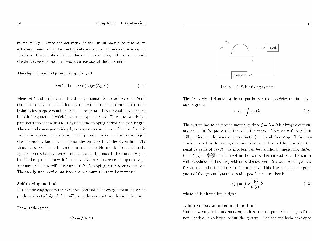
Self-driving method

In a self-driving system the available information at every instant is used to

produce a control signal that will drive the system towards an optimum.

For a static system

y(t) = f(u(t))

11

u

y

dy/dt

Integrator

Figure 1.2. Self driving system

The �rst order derivative of the output is then used to drive the input via

an integrator

u(t) =Z

_y(t)dt (1.2)

The system has to be started manually, since _y = _u = 0 is always a station-

ary point. If the process is started in the correct direction with _u 6= 0, it

will continue in the same direction until _y = 0 and then stop. If the pro-

cess is started in the wrong direction, it can be detected by observing the

negative value of dy=dt. the problem can be handled by measuring du=dt,

then f 0(u) = dy=dt

du=dtcan be used in the control law instead of _y. Dynamics

will introduce the further problem to the system. One way to compensate

for the dynamics is to �lter the input signal. This �lter should be a good

guess of the system dynamics, and a possible control law is

u(t) =Z

k_y(t)

_u�(t)dt (1.3)

where u� is �ltered input signal.

Adaptive extremum control methods

Until now only little information, such as the output or the slope of the

nonlinearity, is collected about the system. For the methods developed

12 Chapter 1. Introduction

later on, the control action is calculated from a model obtained by some

kind of identi�cation. The input may be chosen as the estimated extremum

position. For this type of methods, each control action is preceded by an

identi�cation phase. Based on the estimates a control step is then taken,

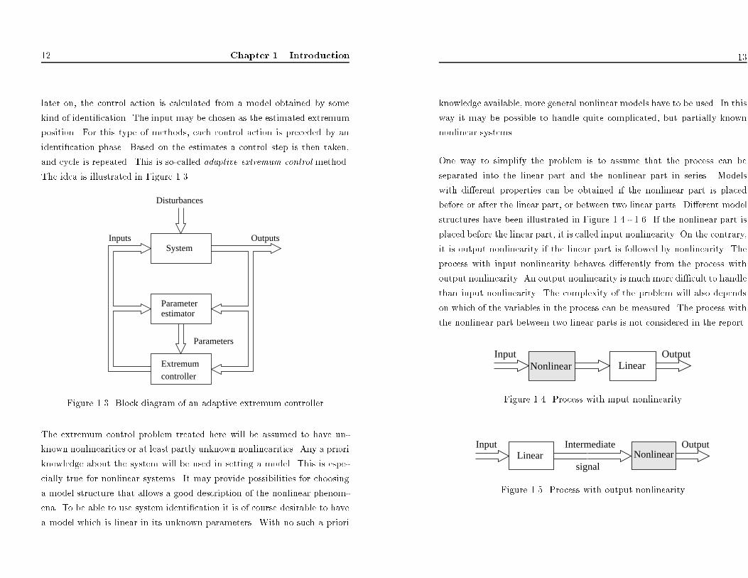
and cycle is repeated. This is so-called adaptive extremum control method.

The idea is illustrated in Figure 1.3.

Outputs

Parameterestimator

Extremumcontroller

System

Disturbances

Parameters

Inputs

Figure 1.3. Block diagram of an adaptive extremum controller

The extremum control problem treated here will be assumed to have un-

known nonlinearities or at least partly unknown nonlinearities. Any a priori

knowledge about the system will be used in setting a model. This is espe-

cially true for nonlinear systems. It may provide possibilities for choosing

a model structure that allows a good description of the nonlinear phenom-

ena. To be able to use system identi�cation it is of course desirable to have

a model which is linear in its unknown parameters. With no such a priori

13

knowledge available, more general nonlinear models have to be used. In this

way it may be possible to handle quite complicated, but partially known

nonlinear systems.

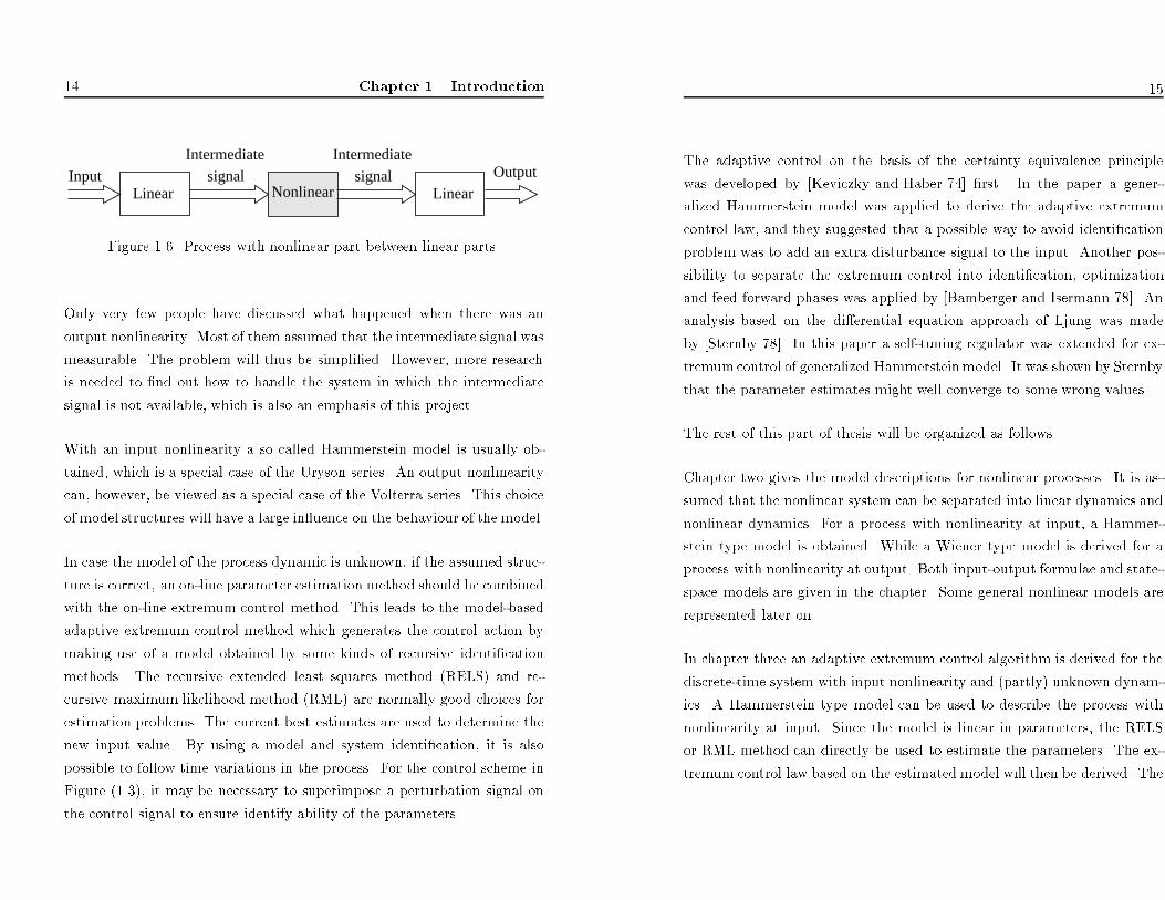
One way to simplify the problem is to assume that the process can be

separated into the linear part and the nonlinear part in series. Models

with di�erent properties can be obtained if the nonlinear part is placed

before or after the linear part, or between two linear parts. Di�erent model

structures have been illustrated in Figure 1.4 - 1.6. If the nonlinear part is

placed before the linear part, it is called input nonlinearity. On the contrary,

it is output nonlinearity if the linear part is followed by nonlinearity. The

process with input nonlinearity behaves di�erently from the process with

output nonlinearity. An output nonlinearity is much more di�cult to handle

than input nonlinearity. The complexity of the problem will also depends

on which of the variables in the process can be measured. The process with

the nonlinear part between two linear parts is not considered in the report.

NonlinearInput Output

Linear

Figure 1.4. Process with input nonlinearity

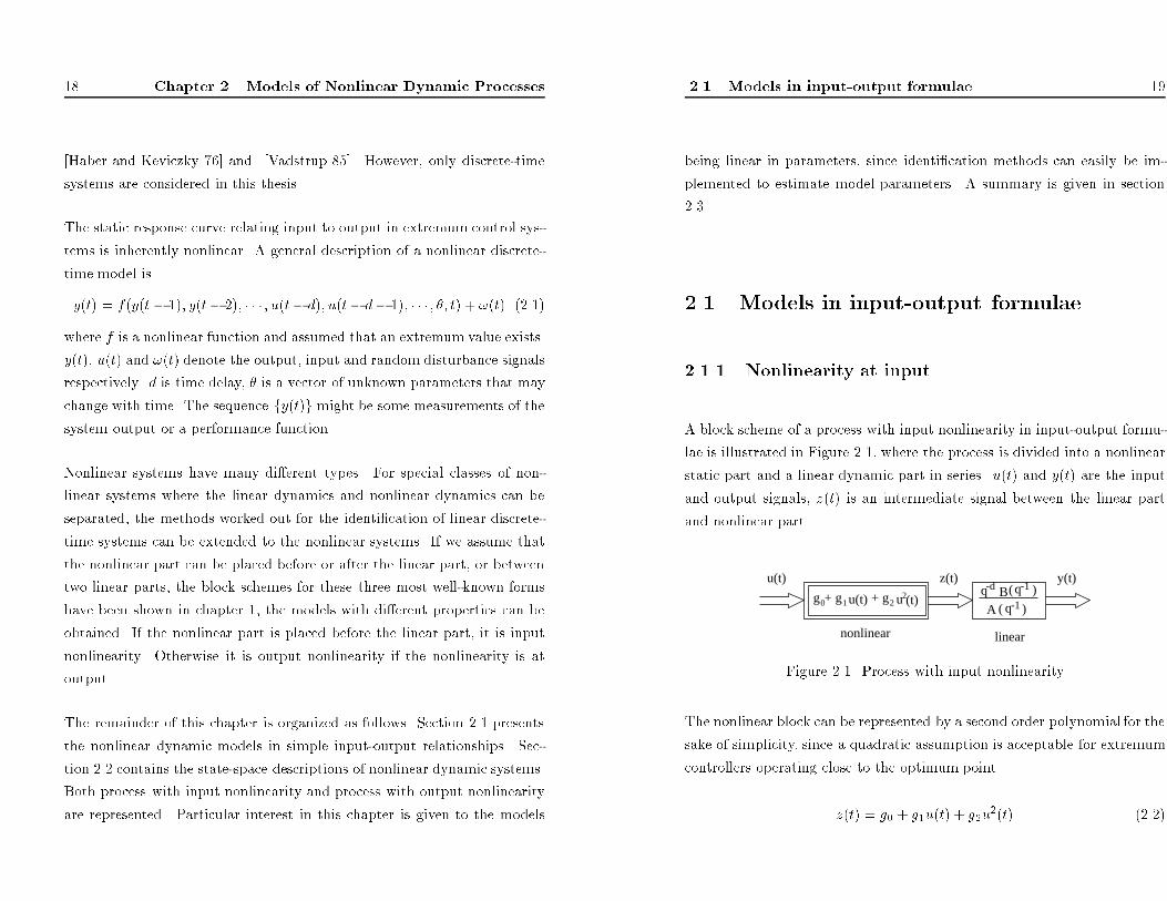
OutputInput Intermediate

signalNonlinearLinear

Figure 1.5. Process with output nonlinearity

14 Chapter 1. Introduction

InputLinear

IntermediateIntermediatesignal

Nonlinearsignal

LinearOutput

Figure 1.6. Process with nonlinear part between linear parts.

Only very few people have discussed what happened when there was an

output nonlinearity. Most of them assumed that the intermediate signal was

measurable. The problem will thus be simpli�ed. However, more research

is needed to �nd out how to handle the system in which the intermediate

signal is not available, which is also an emphasis of this project.

With an input nonlinearity a so called Hammerstein model is usually ob-

tained, which is a special case of the Uryson series. An output nonlinearity

can, however, be viewed as a special case of the Volterra series. This choice

of model structures will have a large in uence on the behaviour of the model.

In case the model of the process dynamic is unknown, if the assumed struc-

ture is correct, an on-line parameter estimation method should be combined

with the on-line extremum control method. This leads to the model-based

adaptive extremum control method which generates the control action by

making use of a model obtained by some kinds of recursive identi�cation

methods. The recursive extended least squares method (RELS) and re-

cursive maximum likelihood method (RML) are normally good choices for

estimation problems. The current best estimates are used to determine the

new input value. By using a model and system identi�cation, it is also

possible to follow time variations in the process. For the control scheme in

Figure (1.3), it may be necessary to superimpose a perturbation signal on

the control signal to ensure identify ability of the parameters.

15

The adaptive control on the basis of the certainty equivalence principle

was developed by [Keviczky and Haber 74] �rst. In the paper a gener-

alized Hammerstein model was applied to derive the adaptive extremum

control law, and they suggested that a possible way to avoid identi�cation

problem was to add an extra disturbance signal to the input. Another pos-

sibility to separate the extremum control into identi�cation, optimization

and feed forward phases was applied by [Bamberger and Isermann 78]. An

analysis based on the di�erential equation approach of Ljung was made

by [Sternby 78]. In this paper a self-tuning regulator was extended for ex-

tremumcontrol of generalized Hammersteinmodel. It was shown by Sternby

that the parameter estimates might well converge to some wrong values.

The rest of this part of thesis will be organized as follows.

Chapter two gives the model descriptions for nonlinear processes. It is as-

sumed that the nonlinear system can be separated into linear dynamics and

nonlinear dynamics. For a process with nonlinearity at input, a Hammer-

stein type model is obtained. While a Wiener type model is derived for a

process with nonlinearity at output. Both input-output formulae and state-

space models are given in the chapter. Some general nonlinear models are

represented later on.

In chapter three an adaptive extremum control algorithm is derived for the

discrete-time system with input nonlinearity and (partly) unknown dynam-

ics. A Hammerstein type model can be used to describe the process with

nonlinearity at input. Since the model is linear in parameters, the RELS

or RML method can directly be used to estimate the parameters. The ex-

tremum control law based on the estimated model will then be derived. The

16

Chapter1.Introduction

inputsignaltotheprocessischosenastheestimatedpositionoftheopti-

mumwithasuperimposedperturbationsignalwhichassuresthepersistent

excitationoftheprocess.Twoexamplesaregiventoassesstheperformance

ofalgorithm.Theconvergencepropertiesofthealgorithmareanalysedby

usingtheODEapproach.

Chapterfourconcernstheprocesswithnonlinearityatoutput.Theex-

tremumcontrolproblemisingeneralmuchdi�culttohandleinthiscase.

However,aspecialcaseiswhentheintermediatesignalbetweenthelinear

andnonlinearpartcanbemeasured.Theproblemwillbesimpli�ed.The

identi�cationcanbeimplementedforlinearpartandnonlinearpartsepa-

rately,andtheextremumcontrollawcanthenbederivedbasedonstatic

optimizationofaperformancefunction.Whentheintermediatesignalisnot

measurable,theemphasiswillgivetotheparameteridenti�cation,sincethe

extremumcontrollawreliesheavilyontheestimatedmodel.Theextended

Kalman�lter(EKF)methodusedasajointparameterandstateestimator

isimplementedforanonlinearstate-spacemodel.Therecursivepredic-

tionerrormethodandtherecursivelinesearchpredictionerrormethodare

derivedforanonlinearinnovationsmodel.Thebehaviourofthedi�erent

estimationmethodsisinvestigatedbysimulationexamples.

Chapter�vegivessummaryandconclusionsoftheinvestigationsinthe

previouschapters.

Chapter2

ModelsofNonlinear

DynamicProcesses

Asitismentionedinchapter1,thekeypointofextremumcontrolisthe

basicassumptionofamodelwhichdescribestheperformancefunctionor

theprocessdynamics.Themostimportantfeatureisthattheprocessis

assumedtobenonlinear,andthebiggestproblemisthentochooseaproper

modelstructure,sincethemodel-basedextremumcontrolmethodsgenerate

thecontrolactionbymakinguseofamodelobtainedbysomekindof

identi�cationmethod.

Themathematicaldescriptionsofthenonlinearsystemshavebeenthe

subjectinmanyarticles.Somefrequentlyappliedmodelsaregivenby

17

18 Chapter 2. Models of Nonlinear Dynamic Processes

[Haber and Keviczky 76] and [Vadstrup 85]. However, only discrete-time

systems are considered in this thesis.

The static response curve relating input to output in extremum control sys-

tems is inherently nonlinear. A general description of a nonlinear discrete-

time model is

y(t) = f(y(t � 1); y(t� 2); � � � ; u(t� d); u(t� d� 1); � � � ; �; t) + !(t) (2.1)

where f is a nonlinear function and assumed that an extremum value exists.

y(t), u(t) and !(t) denote the output, input and random disturbance signals

respectively. d is time delay, � is a vector of unknown parameters that may

change with time. The sequence fy(t)g might be some measurements of the

system output or a performance function.

Nonlinear systems have many di�erent types. For special classes of non-

linear systems where the linear dynamics and nonlinear dynamics can be

separated, the methods worked out for the identi�cation of linear discrete-

time systems can be extended to the nonlinear systems. If we assume that

the nonlinear part can be placed before or after the linear part, or between

two linear parts, the block schemes for these three most well-known forms

have been shown in chapter 1, the models with di�erent properties can be

obtained. If the nonlinear part is placed before the linear part, it is input

nonlinearity. Otherwise it is output nonlinearity if the nonlinearity is at

output.

The remainder of this chapter is organized as follows. Section 2.1 presents

the nonlinear dynamic models in simple input-output relationships. Sec-

tion 2.2 contains the state-space descriptions of nonlinear dynamic systems.

Both process with input nonlinearity and process with output nonlinearity

are represented. Particular interest in this chapter is given to the models

2.1 Models in input-output formulae 19

being linear in parameters, since identi�cation methods can easily be im-

plemented to estimate model parameters. A summary is given in section

2.3.

2.1 Models in input-output formulae

2.1.1 Nonlinearity at input

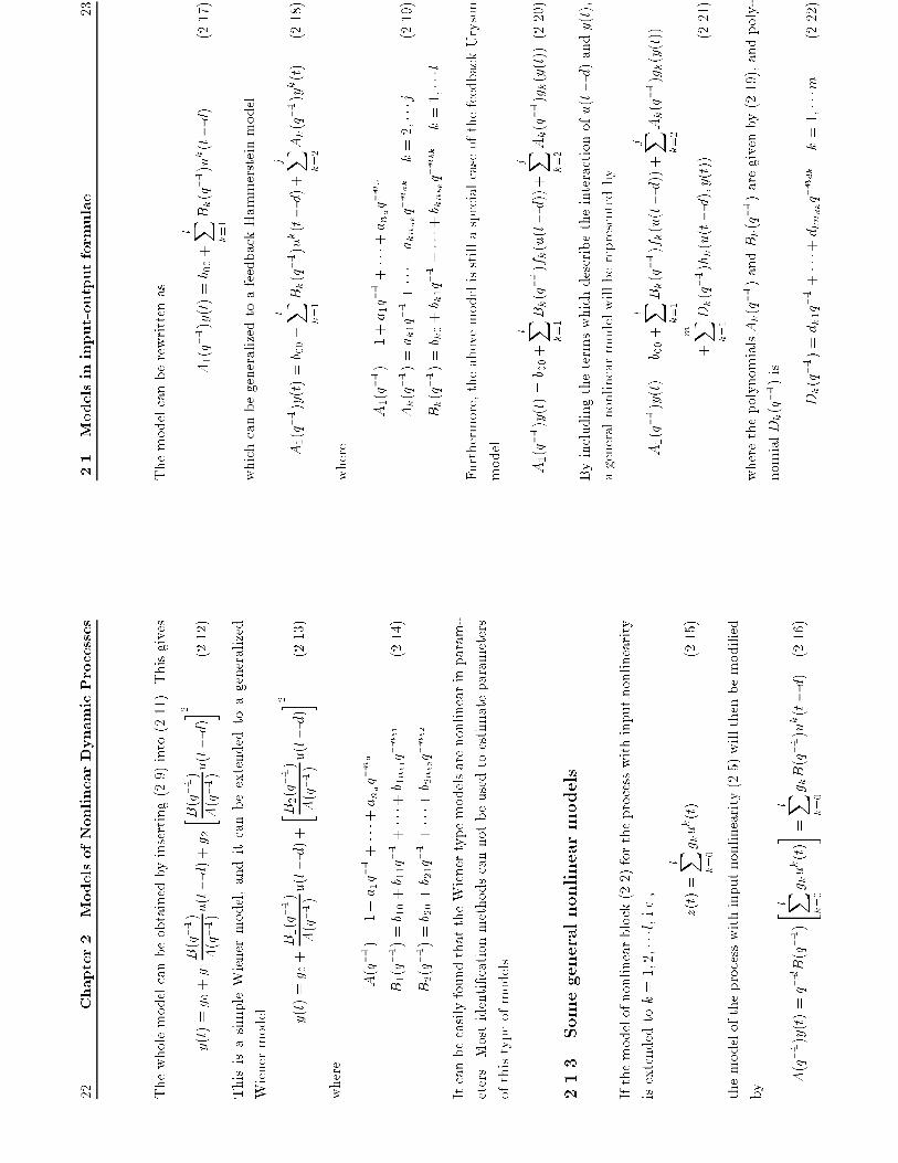
A block scheme of a process with input nonlinearity in input-output formu-

lae is illustrated in Figure 2.1, where the process is divided into a nonlinear

static part and a linear dynamic part in series. u(t) and y(t) are the input

and output signals, z(t) is an intermediate signal between the linear part

and nonlinear part.

y(t)B q )-1(-dqq-1A

(t))(

z(t)

linear

u(t)

nonlinear

g0+ g1 u(t) + g2 u2

Figure 2.1. Process with input nonlinearity

The nonlinear block can be represented by a second order polynomial for the

sake of simplicity, since a quadratic assumption is acceptable for extremum

controllers operating close to the optimum point.

z(t) = g0 + g1u(t) + g2u2(t) (2.2)

20 Chapter 2. Models of Nonlinear Dynamic Processes

The linear block can be obtained by describing it as a linear di�erence

equation

A(q�1)y(t) = q�dB(q�1)z(t) (2.3)

where d is time delay, and

A(q�1) = 1 + a1q�1 + � � �+ anaq�na

B(q�1) = b0 + b1q�1 + � � �+ bnbq�nb (2.4)

are the polynomials in backward shift operator q�1.

Combining two models gives the representation for the whole process

A(q�1)y(t) = q�dB(q�1)[g0 + g1u(t) + g2u2(t)]

= g0 �B + g1B(q�1)u(t� d) + g2B(q�1)u2(t � d)(2.5)

where �B = B(1). This is a simple Hammerstein model that can be extended

to a generalized Hammerstein model

A(q�1)y(t) = b00 +B1(q�1)u(t� d) +B2(q�1)u2(t� d) (2.6)

where

A(q�1) = 1 + a1q�1 + � � �+ anaq�na

B1(q�1) = b10 + b11q�1 + � � �+ b1nb1q�nb1 (2.7)

B2(q�1) = b20 + b21q�1 + � � �+ b2nb2q�nb2

Thus we get a system equation which is linear in parameters and can directly

be written in regressive form

y(t) = 'T (t)� (2.8)

where � is the parameter vector, '(t) is a vector which includes previous

input and output signals.

2.1 Models in input-output formulae 21

The models of Hammerstein type have been used quite often in extremum

control systems. The Hammerstein representation is very popular since it is

a good picture of the reality, and linear in terms of the unknown parameters

of the system. Most identi�cation methods are based on the assumption

that the model is linear in parameters.

2.1.2 Nonlinearity at output

For the general description of the nonlinear model in input-output formula

(2.1), if the process has the nonlinearity at output, the model can then be

illustrated by Figure 2.2.

z(t)u(t)B q )-1(-dqq-1 (t)

A )(

linear

y(t)

nonlinear

g0+ g1z(t) + g2 z2

Figure 2.2. Process with output nonlinearity

For an output nonlinearity, the model of linear block can be written as

A(q�1)z(t) = q�dB(q�1)u(t) (2.9)

where

A(q�1) = 1 + a1q�1 + � � �+ anaq�na

B(q�1) = b0 + b1q�1 + � � �+ bnbq�nb (2.10)

The model of the nonlinear block is given by

y(t) = g0 + g1z(t) + g2z2(t) (2.11)

22

Chapter2.ModelsofNonlinearDynamicProcesses

Thewholemodelcanbeobtainedbyinserting(2.9)into(2.11).Thisgives

y(t)=g 0+g 1

B(q�1)

A(q�1)

u(t�d)+g 2

� B(q�1)

A(q�1)

u(t�d)� 2(2.12)

ThisisasimpleWienermodel,anditcanbeextendedtoageneralized

Wienermodel y

(t)=g 0+

B1(q�1)

A(q�1)

u(t�d)+

� B 2(q�1)

A(q�1)

u(t�d)� 2(2.13)

where

A(q�1)=1+a1q�1+���+anaq�na

B1(q�1)=b 10+b 11q�1+���+b 1nb1

q�nb1

(2.14)

B2(q�1)=b 20+b 21q�1+���+b 2nb2

q�nb2

ItcanbeeasilyfoundthattheWienertypemodelsarenonlinearinparam-

eters.Mostidenti�cationmethodscannotbeusedtoestimateparameters

ofthistypeofmodels.

2.1.3

Somegeneralnonlinearmodels

Ifthemodelofnonlinearblock(2.2)fortheprocesswithinputnonlinearity

isextendedtok=1;2;���l,i.e.,

z(t)=

l X k=0

g kuk(t)

(2.15)

themodeloftheprocesswithinputnonlinearity(2.5)willthenbemodi�ed

by

A(q�1)y(t)=q�dB(q�1)

" l X k=0

g kuk(t)# =

l X k=0

g kB(q�1)uk(t�d)

(2.16)

2.1

Modelsininput-outputformulae

23

Themodelcanberewrittenas

A1(q�1)y(t)=b 00+

l X k=1

Bk(q�1)uk(t�d)

(2.17)

whichcanbegeneralizedtoafeedbackHammersteinmodel

A1(q�1)y(t)=b 00+

l X k=1

Bk(q�1)uk(t�d)+

j X k=2

Ak(q�1)yk(t)

(2.18)

where

A1(q�1)=1+a1q�1+���+anaq�na

Ak(q�1)=ak1q�1+���+aknakq�nak

k=2;���j

(2.19)

Bk(q�1)=b k0+b k1q�1+���+b knbkq�nbk

k=1;���l

Furthermore,theabovemodelisstillaspecialcaseofthefeedbackUryson

model

A1(q�1)y(t)=b 00+

l X k=1

Bk(q�1)fk(u(t�d))+

j X k=2

Ak(q�1)gk(y(t))(2.20)

Byincludingthetermswhichdescribetheinteractionofu(t�d)andy(t),

ageneralnonlinearmodelwillberepresentedby

A1(q�1)y(t)=b 00+

l X k=1

Bk(q�1)fk(u(t�d))+

j X k=2

Ak(q�1)gk(y(t))

+

m X k=1

Dk(q�1)hk(u(t�d);y(t))

(2.21)

wherethepolynomialsAk(q�1)andBk(q�1)aregivenby(2.19),andpoly-

nomialDk(q�1)is

Dk(q�1)=dk1q�1+���+dkndkq�ndk

k=1;���m

(2.22)

24 Chapter 2. Models of Nonlinear Dynamic Processes

In Uryson model (2.20), function fk and gk depend only on u(t � d) and

y(t). If we wish to generalize it, another type of model, the Volterra model,

can also be used to model the process with output nonlinearity. For the

sake of simplicity, only model of second degree are presented

A1(q�1)y(t) = g0 + B1(q�1)u(t) +

lXk=0

B2k(q�1)u(t)u(t� k)

+

jXk=0

A2k(q�1)y(t)y(t � k) (2.23)

where

A1(q�1) = 1 + a11q�1 + � � �+ a1na1q�na

B1(q�1) = b10 + b11q�1 + � � �+ b1nb1q�nb1

A2k(q�1) = a2k1q�1 + � � �+ aak(j�k)q�(j�k)

B2k(q�1) = b2k0 + b2k1q�1 + � � �+ b2k(l�k)q�(l�k)

(2.24)

This is called the second order feedback Volterra model.

2.2 Models in state-space formulae

2.2.1 Nonlinearity at input

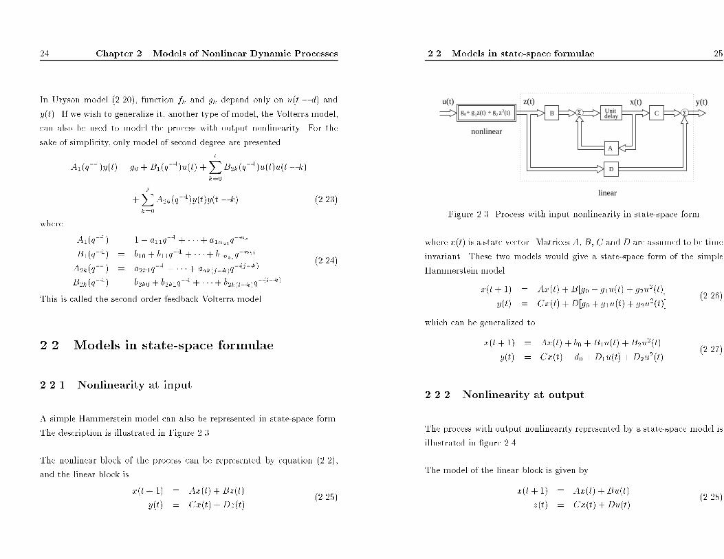
A simple Hammerstein model can also be represented in state-space form.

The description is illustrated in Figure 2.3.

The nonlinear block of the process can be represented by equation (2.2),

and the linear block isx(t+ 1) = Ax(t) + Bz(t)

y(t) = Cx(t) +Dz(t)

(2.25)

2.2 Models in state-space formulae 25

C Σ

y(t)

delayUnitΣB

A

D

linear

x(t)g0+ g1z(t) + g2 z2(t)

nonlinear

z(t)u(t)

Figure 2.3. Process with input nonlinearity in state-space form

where x(t) is a state vector. Matrices A, B, C andD are assumed to be time

invariant. These two models would give a state-space form of the simple

Hammerstein model

x(t+ 1) = Ax(t) + B[g0 + g1u(t) + g2u2(t)]

y(t) = Cx(t) +D[g0 + g1u(t) + g2u2(t)]

(2.26)

which can be generalized to

x(t+ 1) = Ax(t) + b0 + B1u(t) +B2u2(t)

y(t) = Cx(t) + d0 +D1u(t) +D2u2(t)

(2.27)

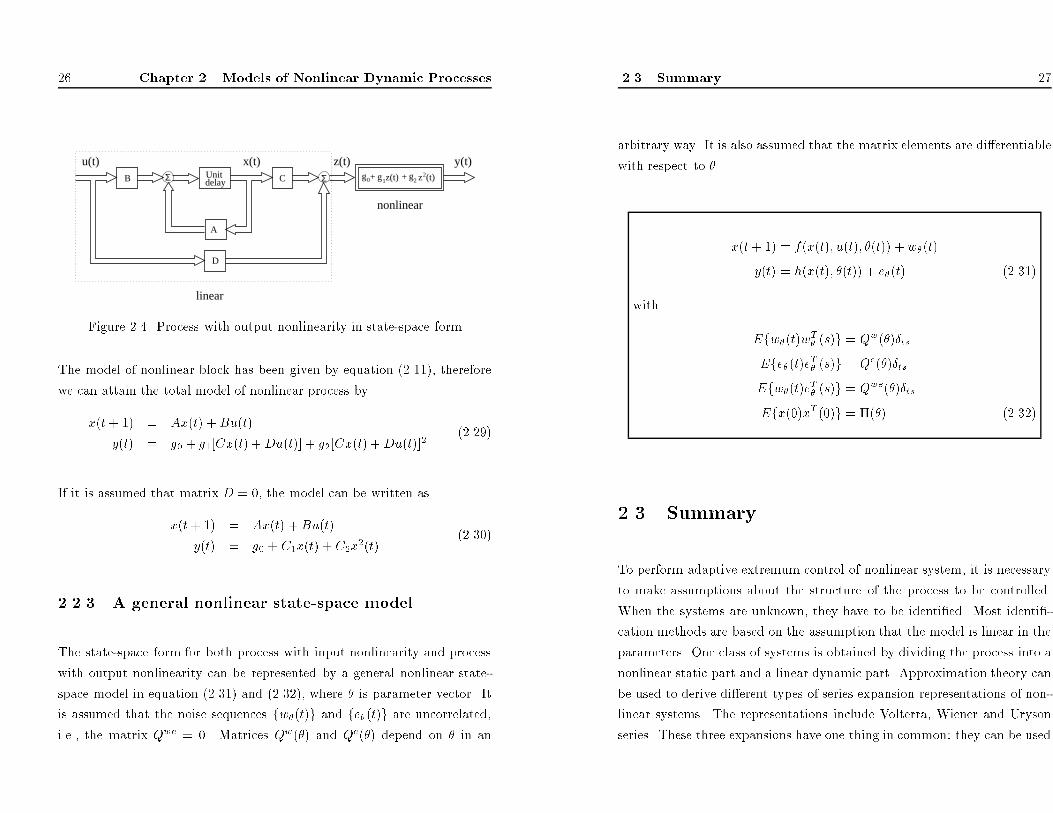
2.2.2 Nonlinearity at output

The process with output nonlinearity represented by a state-space model is

illustrated in �gure 2.4.

The model of the linear block is given by

x(t+ 1) = Ax(t) +Bu(t)

z(t) = Cx(t) +Du(t)

(2.28)

26 Chapter 2. Models of Nonlinear Dynamic Processes

g0

x(t)+ g1z(t) + g2 z2(t)C Σdelay

UnitΣB

A

D

y(t)

linear

nonlinear

u(t) z(t)

Figure 2.4. Process with output nonlinearity in state-space form

The model of nonlinear block has been given by equation (2.11), therefore

we can attain the total model of nonlinear process by

x(t+ 1) = Ax(t) +Bu(t)

y(t) = g0 + g1[Cx(t) +Du(t)] + g2[Cx(t) +Du(t)]2

(2.29)

If it is assumed that matrix D = 0, the model can be written as

x(t+ 1) = Ax(t) +Bu(t)

y(t) = g0 + C1x(t) + C2x2(t)

(2.30)

2.2.3 A general nonlinear state-space model

The state-space form for both process with input nonlinearity and process

with output nonlinearity can be represented by a general nonlinear state-

space model in equation (2.31) and (2.32), where � is parameter vector. It

is assumed that the noise sequences fw�(t)g and fe�(t)g are uncorrelated,

i.e., the matrix Qwe = 0. Matrices Qw(�) and Qe(�) depend on � in an

2.3 Summary 27

arbitrary way. It is also assumed that the matrix elements are di�erentiable

with respect to �.x(t+ 1) = f(x(t); u(t); �(t)) +w�(t)

y(t) = h(x(t); �(t)) + e�(t) (2.31)

with

Efw�(t)wT� (s)g = Qw(�)�ts

Efe�(t)eT� (s)g = Qe(�)�ts

Efw�(t)eT� (s)g = Qwe(�)�ts

Efx(0)xT (0)g = �(�) (2.32)

2.3 Summary

To perform adaptive extremum control of nonlinear system, it is necessary

to make assumptions about the structure of the process to be controlled.

When the systems are unknown, they have to be identi�ed. Most identi�-

cation methods are based on the assumption that the model is linear in the

parameters. One class of systems is obtained by dividing the process into a

nonlinear static part and a linear dynamic part. Approximation theory can

be used to derive di�erent types of series expansion representations of non-

linear systems. The representations include Volterra, Wiener and Uryson

series. These three expansions have one thing in common: they can be used

28

Chapter2.ModelsofNonlinearDynamicProcesses

tomodelprocesseswherelineardynamicsisfollowedbyanonlinearity.The

Urysonseriescan,however,alsoincludenonlinearitiesattheinput.Aspe-

cialcaseofUrysonseriesisrepresentedbyHammersteinmodels,whichhave

theadvantagethatthemodelislinearintheparameters.

Chapter3

InputNonlinearity

Theideaofanextremumcontrollerwhichcombinesarecursiveestimation

algorithmwithasynthesisalgorithmwillbeinvestigatedinthischapterfora

processwithinputnonlinearity.Withthenonlinearityattheinputitiseasy

tosetupamodelwhichislinearintheparameters,andthusdirectlylends

itselftoparameterestimationandadaptivecontrol.Theextremumcontrol

lawisderivedbasedonstaticoptimizationofaperformancefunction.This

isanimportantpracticalproblem,sinceanumberofindustrialprocessesare

suchthattheirperformancecanbeimprovedbyadjustingplantvariables

soastoincreasethee�ciencyoftheprocesses.

Inordertosimplifythenotationsandanalysis,onlyaspecialloworder

caseofthemodelwillbetaken.Thesystemconsideredisofasecondorder

Hammersteinmodelwithorwithoutdynamics.Theprocesswithhigher

orderdynamicmodelcanbetreatedinthesimilarway.

29

30

Chapter3.InputNonlinearity

Someoptimizationbackgroundconsideredtobeofparticularrelevanceto

theextremumcontrolproblemsisgiveninAppendix

A.Thealgorithms

includethehill-climbingmethod,gradientmethod,NewtonandGauss-

Newtonmethod.Theextremum

controllawderivedinthischaptercan

beconsideredasadirectimplementationoftheNewtoniteration.

Whenthesystemdynamicisunknown,themodelhastobeidenti�ed.An

identi�cationmethod,e.g.,therecursiveextendedleastsquaresmethod,for

theHammersteintypemodelswillbepresented.Basedonthecurrentbest

estimatedparameters,anon-lineextremumcontrollawisderived.

Thischapterisorganizedasfollows.Section3.1isconcernedwithadaptive

extremumcontrolfortheprocesswithinputnonlinearity.Someexamples

aregiventoillustratetheperformanceofthealgorithminsection3.2.The

convergencepropertyofthealgorithmisdiscussedinsection3.3.Thesum-

maryandconclusionsaregiveninsection3.4.

3.1

Adaptiveextremum

controlforHammersteinmodel

31

3.1

Adaptiveextremum

controlforHammer-

steinmodel

3.1.1

Themodi�edHammersteinmodel

Inmanyinvestigationsofextremumcontrolsystemsitisassumedthatthe

systemsarestatic,i.e.,inputsignalhasonlyaninstantaneouse�ect.This

assumptioncanbejusti�edifthetimebetweenthechangesinthereference

valueissu�cientlylong.Atypicaldescriptionofthestaticsystemis

y(t)=b 0+B1(q�1)u(t�d)+B2(q�1)u2(t�d)+!(t)

(3.1)

Iftherearedynamicsintheprocess,theinputsignalwillin uencethesys-

tembehaviouratsubsequenttimes.Itmeansthattheperformancemaynot

havesettledatnewsteady-statevaluebeforethenextmeasurementistaken.

Thiswillgiveaninteractioninthecontrolsystem.Thecorrelationandin-

teractionbetweendi�erentmeasurementsoftheperformancewillconfuse

theoptimizationroutine.Thereforeitisnecessarytotakethedynamicsinto

considerationwhendoingtheoptimization.Onepossibilitydiscussedabove

istowaituntilthetransientshavevanishedbeforethenextchangeismade.

Ofcourse,thiswillincreasetheconvergencetime,especiallyiftheprocess

haslongtimeconstants.Anotherwayaroundtheproblemistobasethe

optimizationonnonlineardynamicmodel[� Astr�omandWittenmark89].

AnonlineardynamicmodelofHammersteintypefortheprocesswithinput

nonlinearityhasbeengivenin(2.6)inchapter2.Tobemorespeci�c,ifthe

measurementsofprocessoutputorperformanceistypicallycorruptedby

32

Chapter3.InputNonlinearity

noise,itisthennecessarytotakethenoisemodelintoaccount.Therefore

thegeneralizedHammersteinmodel(2.6)ismodi�edby

A(q�1)y(t)=b 0+B1(q�1)u(t�d)+B2(q�1)u

2(t�d)+C(q�1)e(t)

(3.2)

with

A(q�1)=1+a1q�1+���+anaq�na

B1(q�1)=b 10+b 11q�1+���+b 1nb1

q�nb1

B2(q�1)=b 20+b 21q�1+���+b 2nb2

q�nb2

C(q�1)=1+c 1q�1+���+c ncq�nc

whereu(t),andy(t)aretheinputandoutputsignals,e(t)isawhitenoise

withzeromeannormaldistribution.

3.1.2

Extremum

controllaw

Thepurposeoftheextremumcontrolistomaintaintheoutputascloseas

possibletotheextremumdespitethein uenceofdisturbances.Itmeans

thatthecontrolobjectiveistomaximizeorminimizetheperformancefunc-

tion

J(u(t))=Efy(t+d)g

(3.3)

whereEdenotestheexpectationoperator,y(t)istheoutputsignaloraper-

formancefunction.IfitisassumedthattheperformancefunctionJ(�)has

the�rstandsecondorderderivatives,thecontrollawcanthenbeachieved

3.1

Adaptiveextremum

controlforHammersteinmodel

33

by

dJ d

u=0

(3.4)

Admissiblecontrollawmayusealltheinformationavailable,i.e.,u(t)may

dependony(t)andallpreviousinputsandoutputs.

Considerasystem

withinputnonlinearity,whichcanberepresentedby

thegeneralizedHammersteinmodel(3.2),thestaticcharacteristicsofthe

processwillbe

� Ay=b 0+� B1u+� B2u2

(3.5)

Sincetheextremumcontrolistomakethesteady-statevalueofoutputas

loworashighaspossible,theresultingcontrollerwillbederivedfromthe

staticresponsetoseektheoptimalinput.

u(t)=�

� B1

2� B2

(3.6)

andoptimalvalueoftheoutputis

y�=

b 0 � A�

� B2 1

4� A� B2

(3.7)

Theextremumcontrolleristhusaconstantgainandnofeedbackcontroller.

Intheadaptivecaseaconstantgaincontrollerwillreducetheexcitationof

theprocessandidenti�abilitymaybelost.

Theextremumcontrollawcanbeinterpretedasadirectimplementationof

Newtoniteration

u(t+1)=u(t)�

� dy du

� d2y

du2

� u(t)

=u(t)�

� � B 1+2� B2u(t)

2� B2

�

(3.8)

=�

� B1

2� B2

34

Chapter3.InputNonlinearity

Theequivalenceoftheself-tuningadjustmentruleandNewtoniteration

caneasilybeseen.

3.1.3

Parameterestimation

Iftheparametersofthemodelareunknown,theideaistouseanon-line

recursiveestimationproceduretoidentifythem,andateachadjustment

stepusethecurrentbestestimatestodeterminethenewvalueofu(t).

IfC(q�1)=1inthemodel(3.2),theordinaryleast-squaresmethodcan

thenbeuseddirectlytoestimateparameters.IfC(q�1)6=1,itisthen

necessarytoapproximateandusee.g.therecursiveextendedleast-squares

(RELS)methodortherecursivemaximumlikelihood(RML)method.

IfwetakethecaseofC(q�1)6=1,themodel(3.2)canbewrittenas

y(t)='T(t)�+�(t)

(3.9)

where '

(t)=[�y(t�1);���;�y(t�na);1;u(t�d);���;u(t�nb1�d);

u2(t�d);���;u2(t�nb2�d);�(t�1);���;�(t�nc)]T

(3.10)

�=[a1;���;ana;b0;b10;���;b1nb1;b20;���;b2nb2;c1;���;c nc]T

and

�(t)=y(t)�'T(t)^ �(t�1)

(3.11)

TheestimatesusingRELSmethodaregivenbyequations

3.1

Adaptiveextremum

controlforHammersteinmodel

35

^y(t)='T(t)^ �(t�1)

^ �(t)=^ �(t�1)+k(t)[y(t)�^y(t)]

k(t)=P(t)'(t)[�(t)+'T(t)P(t)'(t)]�1

P(t+1)=[I�k(t)'T(t)]P(t)=�(t)

(3.12)

where�(t)isanexponentialforgettingfactor.

Itisthenpossibletomakeadirectadaptiveextremumcontrollerforthe

processdiscussedinthischapter.Theestimatedparametersmaythenbe

usedinthecontrollaw(3.6)insteadofthetrueparametervalues

u(t)=�

^ � B1(t)

2^ � B2(t)

(3.13)

where�^ � B1(t)=2^ � B2(t)isthecurrentestimatedvalueoftheoptimalinput.

Thisleadstoacertaintyequivalencecontroller.

3.1.4

Theadaptiveextremum

controlalgorithm

Theon-lineparameterestimatorcombinedwithon-lineextremumcontroller

leadstoanadaptiveextremumcontrollerwhichcanbesummarizedas

36 Chapter 3. Input Nonlinearity

Step 1: Apply input u(t) to the nonlinear system and measure the

output y(t).

Step 2: Use RELS or RML algorithm to estimate parameters for the

model (3.2).

Step 3: The extremum control law is

u(t+ 1) = �^�B1(t)

2 ^�B2(t)

Step 4: Increment the time t! t+ 1 and return to Step 1.

Such a scheme has to be used with great care, since the control input de-

pends only on the estimated values. When u(t) is actively varying by large

amounts, i.e., when the self-tuning is in progress, the identi�ability prob-

lems do not arise. When the system is nominally tuned, the u(t) converges

to a constant value. This will reduce the excitation of the process and iden-

ti�ability may be lost, and the parameter estimates may converge to some

wrong values. The problem has been discussed by [Sternby 78]. The re-

port shows that direct application of the certainty equivalence principle to

adaptive extremum control of a Hammerstein type model may cause iden-

ti�cation problems. The estimates will converge to a certain hyper-surface

in the parameter space, but in most cases to other than the true parameter

values.

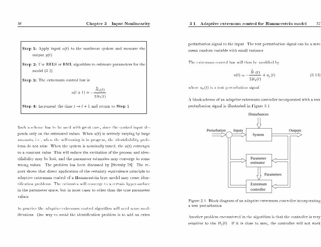
In practice the adaptive extremum control algorithm will need some mod-

i�cations. One way to avoid the identi�cation problem is to add an extra

3.1 Adaptive extremum control for Hammerstein model 37

perturbation signal to the input. The test perturbation signal can be a zero

mean random variable with small variance.

The extremum control law will thus be modi�ed by

u(t) = �^�B1(t)

2 ^�B2(t)+ up(t) (3.14)

where up(t) is a test perturbation signal.

A block scheme of an adaptive extremum controller incorporated with a test

perturbation signal is illustrated in Figure 3.1.

Inputs

Parameterestimator

Extremumcontroller

System

Disturbances

Parameters

OutputsPerturbationFigure 3.1. Block diagramof an adaptive extremum controller incorporating

a test perturbation

Another problem encountered in the algorithm is that the controller is very

sensitive to the ^�B2(t). If it is close to zero, the controller will not work

38

Chapter3.InputNonlinearity

well.Actuallyinmostextremumapplicationtherewillbesomeknowledge

oftheboundsontheparameters.Theboundscanbeusedtoconstrain

theextremumcontrolleractioninoneoftwoways.Eithertheestimated

parameterscanbecheckedagainstknownboundsandconstrainedifnec-

essary,ortheextremumcontrolactioncanbecheckedagainstboundsand

constrainedappropriately.Anotherupdatingformulabasedonstochastic

approximationisgivenby[Sternby78]

u(t+1)=u(t)� (t)[^ � B1(t)+2^ � B2(t)u(t)]

(3.15)

where (t)canbe

(t)=

1 t

(3.16)

or

(t+1)�1= (t)�1+2^ � B2(t+1)

(3.17)

as[KeviczkyandHaber74]suggested.Inserting(3.13)into(3.15)gives

u(t+1)=u(t),andsoitseemsreasonabletobelievethat(3.13)and(3.15)

willbehavesimilarlyiftheestimatesconverge.

Sinceparameterb 0isnotincludedintheextremumcontrollaw,itisthen

notnecessarytoestimateit.Anincrementalformofthemodel(3.2)can

beusedtoeliminatetheconstantcoe�cientb 0,butonlyifthemodel(3.2)

canbemodi�edby

A(q�1)y(t)=b 0+B1(q�1)u(t�d)+B2(q�1)u

2(t�d)+C(q�1)e

(t)

�

(3.18)

whereweassumethatnoisee(t)isadriftdisturbance,and(�

=

1�

q�1)operatorisanintegralactiontocancelthee�ectofthestepoutput

disturbances,e(t)=�

canthenbeconsideredasawhitenoisewithzero

mean.Theinnovationformisthusgivenby

A(q�1)�y(t)=B1(q�1)�u(t�d)+B2(q�1)�u2(t�d)+C(q�1)e(t)(3.19)

3.2

Casestudies

39

where

�y(t)

=

y(t)�y(t�1)

�u(t)

=

u(t)�u(t�1)

�u2(t)

=

u2(t)�u2(t�1)

(3.20)

3.2

Casestudies

Inthissectionthebehaviourofadaptiveextremumcontrolalgorithmdis-

cussedinabovesectionwillbeinvestigatedbysomesimulationexamples.

Example3.1Anonlinearstaticsystem

Itisassumedthatthemodelstructureoftheprocessisknownandanon-

linearstaticsystemisconsideredinthisexample

y(t)=b 0+b 1u(t)+b 2u2(t)+e(t)

(3.21)

Thiscorrespondstoaprocesswithinputnonlinearitywhichisapproximated

byasecondorderpolynomial.Theparametersoftheprocessareb 0=100,

b 1=

2andb 2=

�0:01.Further,e(t)isazeromeanwhitenoisewith

variance1.Themaximumattainablevalueoftheoutputisy�=200,and

optimalinputvalueisu�=100.

Ifitisassumedthattheparametersofthemodelareunknown,thenthey

havetobeestimated.Thelinearregressionusedinestimationis

y(t)='T(t)^ �+�(t)

(3.22)

40

Chapter3.InputNonlinearity

wheretheregressionvectorandparametervectorare

'(t)

=

[1;u(t);u2(t)]T

^ �

=

[^ b0;^ b 1;^ b 2]T

(3.23)

thentheRLSmethodcanbeusedtoestimatetheunknownparameters.

Theextremumcontrollawisthecurrentestimateoftheoptimalpointu�

incorporatedwithanextradisturbancesignalup(t)

u(t)=�

^ b 1(t)

2^ b2(t)

+up(t)

(3.24)

whereaPRBSsignalisselectedastheperturbationsignalup(t)whichen-

suresthepersistentexcitationoftheinputu(t).

010

2030

4050

6070

8090

100

50100

150

Sam

ples

th(1)

010

2030

4050

6070

8090

100

0102030

Sam

ples

th(2)

010

2030

4050

6070

8090

100

−1.

5

−1

−0.

50

Sam

ples

th(3)

Figure3.2.Theestimatedparameters.

3.2

Casestudies

41

010

2030

4050

6070

8090

100

050100

150

Sam

ples

input u(t)

010

2030

4050

6070

8090

100

100

120

140

160

180

200

220

Sam

ples

output y(t) Figure3.3.Thesysteminputandoutput.

TheestimatedparametersareshowninFigure3.2,whereth(1)=

^ b 0,

th(2)=^ b 1andth(3)=^ b 2.Sinceitisassumedtoknowthattheprocess

hasamaximumpoint,theHessianmatrixmustthenbenegativede�nite,

i.e.,^ b 2<0.Thereforetheinitialvalueof^ b 2canbesettoanegativevalue.

TheinputandoutputofthesystemareshowninFigure3.3.

Thesimulationshowsthattheestimatedparametersconvergeveryfasttothe

truevalues.Theextremumcontrollerachievestheoptimalvalueofy�=200

veryquicklyandholdsittherewithminorperturbationswhicharecausedby

thetestperturbationsignalup(t).

3

42

Chapter3.InputNonlinearity

Example3.2Anonlineardynamicsystem

Nowanonlineardynamicsystemisconsidered.Thesystemisassumedto

bedescribedbyasecond-orderHammersteinmodel

y(t)+ay(t�1)=b 0+b 1u(t�1)+b 2u2(t�1)+e(t)

(3.25)

withparametera=

�0:8,andparametersb 0,b 1andb 2havethesame

valuesasexample3.1.Forthisprocess,themaximumattainablevalueof

theprocessoutputisy�=1000andtheoptimalinputisu�=100.

Ifitalltheparametersoftheprocessareunknown,thentheestimation

algorithmhastobeimplemented.Thelinearregression(3.12)canbewritten

by

y(t)='T(t)^ �+�(t)

with

'(t)

=

[�y(t�1);1;u(t�1);u2(t�1)]T

^ �

=

[^a;^ b 0;^ b 1;^ b 2]T

(3.26)

Theextremum

controllawisderivedbymaximizingtheoutputofstatic

responseandtheresultingcontrollerhasthesamestructureasthecontroller

inexample3.1

u(t)=�

^ b 1(t)

2^ b2(t)

+up(t)

andup(t)isaPRBSsignal.

Figure3.4andFigure3.5givetheresultsofsimulation.Theestimated

parametersareshowninFigure3.4,whereth(1)=^a,th(2)=^ b 0,th(3)=^ b 1

andth(4)=

^ b 2.Itcanbeseenthattheestimatedparametersconverge

fast,whileoutputy(t)achievesthemaximum

valueafter20steps.This

3.2

Casestudies

43

isslowerthantheconvergencespeedofestimatedparameters.Theslower

convergencespeediscausedbythedynamicsinthesystem.Inshort,after

initialtransienttheadaptiveextremum

controllerbehavesaswellasthe

controllerinexample3.1.

050

100

−1

−0.

8

−0.

6

−0.

4

−0.

20

Sam

ples

th(1)

050

100

708090100

110

Sam

ples

th(2)

050

100

0510152025

Sam

ples

th(3)

050

100

−1.

5

−1

−0.

50

0.5

Sam

ples

th(4)

Figure3.4.Theestimatedparameters.

010

2030

4050

6070

8090

100

−5005010

0

150

Input u(t)

010

2030

4050

6070

8090

100

0

200

400

600

800

1000

1200

Output y(t)

Sam

ples

Figure3.5.Thesysteminputsandoutputs.

3

44

Chapter3.InputNonlinearity

3.3

Convergenceanalysis

Theconvergencepropertiesoftheextremumcontrollercanbeanalysedby

theOrdinaryDi�erentialEquation(ODE)approachofLjung

[Ljung77].

AbriefsummaryoftheapproachisgiveninAppendixB.

Considerasystem

S:y(t)='T(t)�0+e(t)

(3.27)

andamodelforthesystemis M

:y(t)='T(t)�

(3.28)

theRLSestimatorcanberewrittenas

^ �(t)=^ �(t�1)+P(t)'(t)(y(t)�'T(t)^ �(t�1))

P(t+1)�1=P(t)�1+'(t)'T(t)

(3.29)

Fortheanalysispurposes,wewillintroducethematrixR(t)

R(t)=

1 tP(t)�1

(3.30)

thestandardformofRLSwillthenbetakenas

^ �(t)

=

^ �(t�1)+1 tR(t)�1'(t)[y(t)�'T(t)^ �(t�1)]

R(t)

=

R(t�1)+1 t['(t)'T(t)�R(t�1)]

(3.31)

InordertoformtheODE,�x^ �(t)atsomenominalvalue�andperform

theoperations

f(�)=

limt!1Ef'(t)[y(t)�'T(t)�]g

G(�;R)=

limt!1E['(t)'T(t)�R]

(3.32)

3.3

Convergenceanalysis

45

andthecorrespondingODEisthengivenby

d�

d�

=R�1f(�)

dR d

�=G(�;R)

(3.33)

Ifitisassumedthate(t)inthesystem

isuncorrelatedwith'(t),i.e.,

E['(t)e(t)]=0,inserting(3.27)into(3.32),wehave

f(�)

=

G(�)(� 0��)

G(�;R)

=

G(�)�R

(3.34)

where

G(�)=

limt!1E['(t)'T(t)]

(3.35)

isasymmetricsemi-positivede�nitematrix.

Itcanbeprovedthatif^ �(t)!��andR!R� ,thelocalconvergencepoint

willthensatisfy

f(�� )=

G(�� )(�0���)=0

R�=

G(�� )

(3.36)

IfG(�� )ispositivede�nitematrix,i.e.,

limt!1E['(t)'T(t)]>0

(3.37)

Thisimpliesthat��=

� 0.Thepositivede�niteG(�� )isageneralized

persistentexcitationcondition.Iftheconditionholds,

H(�� )=(R� )�1d d

�f(�)j �=�0

=�I

(3.38)

allofwhoseeigenvaluesareat-1inthelefthalf-plane.Thus,the� 0isthe

onlyconvergencepointunderthepersistentexcitationcondition.

Inadaptiveextremumcontrolalgorithms,Thepersistentlyexcitingofinput

signalisensuredbyadditionofthetestperturbationsignal.

46

Chapter3.InputNonlinearity

Example3.3Convergenceanalysis

WeconsiderthemostsimplecaseofthenonlinearstaticsysteminExample

3.1,wherethesystemiswrittenas

y(t)='T(t)�0+e(t)

(3.39)

where� 0=[b0;b1;b2]T,andmodelisgivenby

y(t)=� 1+� 2u(t)+� 3u2(t)

(3.40)

Thecontrollaw(3.24)istheestimateofextremumlocationu0=��2=2�3,

towhichisaddedaperturbationsignalup(t),then

u(t)=^u0(t)+up(t)

(3.41)

where^u0(t)=�^ �2=2^ � 3.Ifthealgorithmconvergesthen^u0(t)!u0,i.e.,

u(t)=u0+up(t)

(3.42)

Itisassumedthattheperturbationsignalup(t)iszeromeanwhitenoise

withvariance�2 p,i.e.,up(t)2N(0;�2 p),andfurthermoreitisassumedthat

up(t)isindependentofnoisee(t)intheprocess.

ByimplementingtheRLSestimator,iftheestimates^ �(t)!��,wewill

havethatthelocalconvergencepointofODEsatis�es

f(�� )=G(�� )(�0���)=0

R�=G(�)

Itfollowsthat� 1=b 0,� 2=b 1and� 3=b 2aretheuniquelocallystable

convergencepointwiththecondition

G(�)=

� E'(t)'T(t)>0

(3.43)

3.4

Summary

47

i.e.,G(�)ispositivede�niteandH(�� )matrixwillhaveitseigenvaluesat

�1.

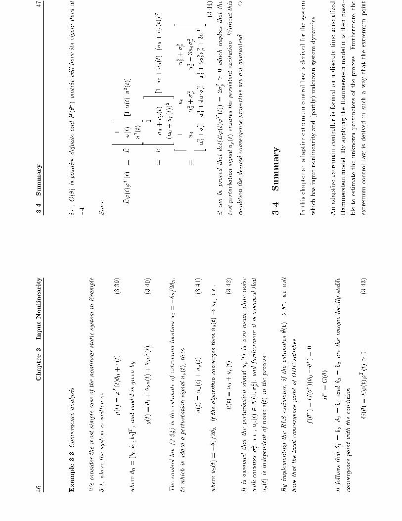
Since � E

'(t)'T(t)

=

� E2 6 6 41

u(t)

u2(t)

3 7 7 5[1u(t)u2(t)]

=

� E2 6 6 41

u0+up(t)

(u0+up(t))2

3 7 7 5[1u0+up(t)(u0+up(t))2]

=

2 6 6 41

u0

u2 0+�2 p

u0

u2 0+�2 p

u3 0+3u0�2 p

u2 0+�2 p

u3 0+3u0�2 p

u4 0+6u2 0�2 p+3�4

3 7 7 5 (3.44)

itcanbeprovedthatdet(� E'(t)'T(t))=2�6 p

>0whichimpliesthatthe

testperturbationsignalup(t)ensuresthepersistentexcitation.Withoutthis

conditionthedesiredconvergencepropertiesarenotguaranteed.

3

3.4

Summary

Inthischapteranadaptiveextremumcontrollawisderivedforthesystem

whichhasinputnonlinearityand(partly)unknownsystemdynamics.

Anadaptiveextremumcontrollerisformedonadiscretetimegeneralized

Hammersteinmodel.ByapplyingtheHammersteinmodelitisthenpossi-

bletoestimatetheunknownparametersoftheprocess.Furthermore,the

extremumcontrollawisderivedinsuchawaythattheextremum

point

48

Chapter3.InputNonlinearity

ofthestaticcharacteristicshouldbechosenineverystep.Theoptimal

controllerisgivenbythecurrentestimateofextremumlocationachieved

byanon-linerecursiveestimationalgorithm.Theidenti�cationproblemis

avoidedbyapplyingthepersistentlyexcitinginput.

Twosimulationexampleshavebeenpresentedtoillustratetheperformance

ofcontrollerandestimator.Thesimulationresultsshowthegoodcon-

vergencepropertiesoftheestimator,andprocessesachievetheextremum

valuesveryfast.Theconvergencepropertiesofthealgorithmhavebeen

analysedbyusingODEapproach.

Chapter4

OutputNonlinearity

Ifthemodelconsistsofadynamiclinearpartandstaticnonlinearpart,

andthelineardynamicsisfollowedbyanonlinearity,itiscalledoutput

nonlinearity.Maybeanoutputnonlinearityisingeneralmoreimportant

thananinputnonlinearityforagooddescriptionofanonlinearsystem.A

nonlinearityatoutputofalinearsystemismuchmoredi�culttohandle

thanoneatinput.Thecomplexityoftheproblemwillalsodependonwhich

ofthevariablesintheprocesscanbemeasured.

Themodelsoftheprocesswithoutputnonlinearityhavebeengivenin

chapter2.Basedonthemodels,anadaptiveextremumcontrollawwillbe

derivedinthischapter.Thentheproblemturnstotwocases:whetherthe

intermediatesignalbetweenthelinearandnonlinearpartcanbemeasured

ornot.Mostdi�cultieswillariseinthesituationwhentheintermediate

signalisnotmeasurable.Thereforewewillgivemoreattentiontothiscase.

49

50

Chapter4.OutputNonlinearity

Thischapterisorganizedasfollows.Theextremumcontrollawisderived

fortheprocesseswithoutputnonlinearityinsection

4.1.Section

4.2is

concernedwiththeadaptiveextremumcontrolofprocesswithoutputnon-

linearityandthemeasuredintermediatedsignal.Thecaseforunmeasured

intermediatesignalisdiscussedinsection

4.3wheretheEKFandRPEM

approachasparameterestimatorswillbeappliedtostate-spacemodels.A

summaryisgiveninsection4.4.

4.1

Basicextremum

controllaw

Foraprocesswithoutputnonlinearitygivenbythemodel(2.9)-(2.11),ifthe

noiseterms�(t)ande(t)enterintheequations,themodelwillbemodi�ed

by

A(q�1)z(t)=B(q�1)u(t�d)+C(q�1)�(t)

(4.1)

y(t)=g 0+g 1z(t)+g 2z2(t)+e(t)

(4.2)

where�(t)ande(t)arezeromeanwhitenoises.Themodeloftheprocess

consistsofanonlinearnoisemodel.

Theextremum

controlobjectiveistomakethesteady-stateresponseof

theoutputatmaximumorminimum.Thecontrollawcanbederivedby

optimizingtheperformancefunction(3.3)insection3.1.

Thesteady-stateresponseoftheprocesswithoutputnonlinearitygivenby

model(4.1)-(4.2)is

� Az

=

� Bu

y

=

g 0+g 1z+g 2z2

(4.3)

4.1

Basicextremum

controllaw

51

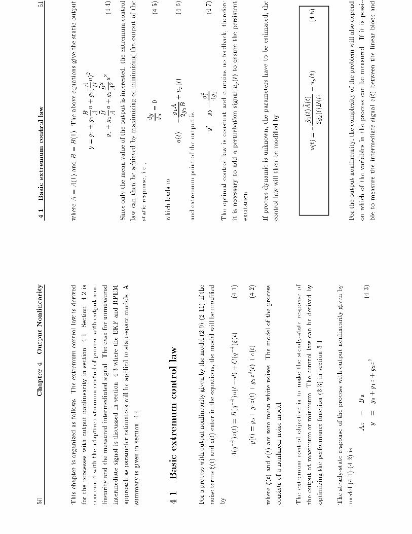
where� A=A(1)and� B=B(1).Theaboveequationsgivethestaticoutput

y=g 0+g 1

� B � Au+g 2(

� A � Bu)2

=g 0+g 1

� B � Au+g 2

� B2 � A

2u2

(4.4)

Sinceonlythemeanvalueoftheoutputisinterested,theextremumcontrol

lawcanthenbeachievedbymaximizingorminimizingtheoutputofthe

staticresponse,i.e.,

dy

du

=0

(4.5)

whichleadsto

u(t)=�

g 1� A

2g2� B+up(t)

(4.6)

andextremumpointoftheoutputis

y�=g 0�

g2 1

4g 2

(4.7)

Theoptimalcontrollawisconstantandcontainsnofeedback,therefore

itisnecessarytoaddaperturbationsignalup(t)toensurethepersistent

excitation.

Ifprocessdynamicisunknown,theparametershavetobeestimated,the

controllawwillthenbemodi�edby

u(t)=�

^g 1(t)^ � A(t)

2^g 2(t)^ � B(t)

+up(t)

(4.8)

Fortheoutputnonlinearity,thecomplexityoftheproblemwillalsodepend

onwhichofthevariablesintheprocesscanbemeasured.Ifitispossi-

bletomeasuretheintermediatesignalz(t)betweenthelinearblockand

52

Chapter4.OutputNonlinearity

nonlinearblock,whichisassumedbymostpeople,thecomplexitywillbe

signi�cantlysimpli�ed.However,moresearchisneededto�ndouthow

tohandlesystemswheretheintermediatesignalisnotavailable.Inthis

case,theproblemismoredi�culttohandle.Thesetwosituationswillbe

discussedseparatelyinthefollowingsections.

4.2

Theintermediatesignalismeasurable

[NavarroandZarrop95]hasgivenanadaptiveextremumcontrolalgorithm

byturningacontrollertooptimizeaperformancefunction

J(u)=Efy(t+d)2g

(4.9)

wherey(t)isprocessoutputgivenby

A(q�1)y(t)=q�1B(q�1)u(t)+e(t)

(4.10)

Inthispaperaperformancefunction(4.9)ratherthananinput-output

model(4.10)isestimated.Thisisactuallyaspecialcaseoftheprocesswith

outputnonlinearityandmeasurableintermediatesignal.Iftheproblemis

comparedtothemodel(4.1)-(4.2),y(t)in(4.10)canthusbeconsidered

asanintermediatesignal,andthemodelofthenonlinearblock(4.2)will

havetheparametersg 0=0,g 1=0,andg 2=1.

Sincetheintermediatesignalcanbemeasured,itisthenpossibletodothe

system

identi�cationforthelinearpartandnonlinearpartseparatelyin-

steadofestimatetheperformancefunction.Theadaptiveextremumcontrol

law(4.8)couldthenbeusedtokeeptheoutputoftheprocessaroundthe

estimatedpositionoftheextremum.

4.2

Theintermediatesignalismeasurable

53

TheRELSalgorithmhasalreadybeengivenin(3.12)inChapter3.The

modeloflinearpartusedinparameterestimationiswrittenasalinear

regression

z(t)='T 1(t)�1+�(t)

(4.11)

with '

1(t)

=

[�z(t�1);����z(t�na);u(t�d);���u(t�d�nb);

�(t�1);���;�(t�nc)]T

� 1

=

[a1;���ana;b1;���;bnb;c1;���;c nc]T

(4.12)

Themodelofnonlinearpartis

y(t)='T 2(t)�2+�(t)

(4.13)

where

'2(t)

=

[1;z(t);z2(t)]T

� 2(t)

=

[g0;g 1;g 2]T

(4.14)

Iftheintermediatesignalbetweenthelinearpartandnonlinearpartcan

beknown,theonlydi�erencebetweentheoutputnonlinearityandinput

nonlinearityisthattheinputfortheprocesswithoutputnonlinearityisnot

determineddirectly,butthroughthelineardynamics.Somesimpleexam-

pleswillbegiventoshowthebehaviourofadaptiveextremumcontroller.

Theconvergencepropertiesofthealgorithmcanbeanalysedinthesame

wayasitisgiveninprevioussection.

Example4.1Anunknownnonlineardynamics

Considerasystemwithlinearpart

z(t)+az(t�1)=bu(t�1)+e 1(t)

(4.15)

54

Chapter4.OutputNonlinearity

andnonlinearpart

y(t)=g 0+g 1z(t)+g 2z2(t)+e 2(t)

(4.16)

wherea=�0:8,b=1,g 0=100,g 1=2andg 2=�0:01.Further,e 1(t)

ande 2(t)arezeromeanwhitenoisewithvariances�2 e1=12and�2 e2=0:12

respectively.Themaximumattainablevalueofthesystemoutputis200,the

correspondingoptimalinputis20.

Inthisexampleweassumethatthelineardynamicsoftheprocessisknown,

i.e.,parametersaandbareavailable.Onlyparametersg 0,g 1andg 2for

thenonlinearpartareunknown.Thereforewehavetoestimatethem.The

RLSmethodcandirectlybeusedtoestimatetheparameters.

Basedontheestimatedparameters,theextremumcontrollawisgivenby

u(t)=�

^g 1(t)(1+a)

2^g 2(t)b

+up(t)

(4.17)

whereup(t)isperturbationsignal.Theextremumcontrollawisdetermined

byboththelineardynamicsandnonlineardynamics.Theperturbationsig-

nalisactuallynotnecessaryinthiscase,sincethenoiseontheintermediate

signale 1(t)actsasaperturbationsignalandimprovestheidenti�ability.

TheestimatedparametersareshowninFigure4.1whereth(1)=^g 0,th(2)=

^g 1andth(3)=^g 2.Figure4.2givestheinputu(t),outputy(t)andinter-

mediatesignalz(t).Theestimatedparametersconvergetothetruevalue

veryfast.Theoutputachievesthemaximumvalueafter20sec.Simulation

showsgoodconvergencepropertyofadoptiveextremumcontrolalgorithm.

4.2

Theintermediatesignalismeasurable

55

010

2030

4050

6070

8090

100

406080100

th(1)

010

2030

4050

6070

8090

100

0510 th(2)

010

2030

4050

6070

8090

100

−0.

4

−0.

20

th(3)

Sam

ples

Figure4.1.Theestimatedparameters.

010

2030

4050

6070

8090

100

01020 Input u(t)

010

2030

4050

6070

8090

100

050100

150

Intermediate signal z(t)

010

2030

4050

6070

8090

100

100

200

300

Output y(t)

Sam

ples

Figure4.2.Input,outputandintermediatesignal

3

56

Chapter4.OutputNonlinearity

Example4.2Bothlineardynamicsandnonlineardynamicsareunknown

Considertheprocessinexample4.1,ifweassumethatbothparametersin

linearpartandnonlinearpartareunknown,theidenti�cationforlinear

dynamicsandnonlineardynamicswillthenbeimplementedseparately.

Themodelusedtoestimateparametersinlinearpartcanbewrittenin

regressionform(4.11)-(4.12),theregressionvectorandparametervector

are

'1(t)=[�z(t�1);u(t�1)]T

^ � 1=[^a;^ b]T

andthemodelusedtoestimateparametersinnonlinearpartisgivenin

(4.13)-(4.14).

Theextremumcontrollawisidenticalinformwithexample4.1,however

parametersaandbarereplacedbyestimatedvalues

u(t)=�

^g 1(t)(1+^a(t))

2^g 2(t)^ b(t)

+up(t)

(4.18)

wheretheperturbationsignalup(t)isPRBSsignalwhichwillensurethe

identi�abilityofparameter� 1.Thenoisesignalontheintermediatesignal

e 1(t)willensuretheidenti�abilityofparameter� 2.

SimulationsareshowninFigure4.3-Figure4.5.Theestimatedparame-

tersinlinearpartaregiveninFigure4.3whereth1(1)=^aandth1(2)=^ b.

TheestimatedparametersinnonlinearpartaregivenFigure4.4where

th2(1)=

^g 0,th2(2)=

^g 1andth2(3)=

^g 3.Theinputu(t),outputy(t)

andintermediatesignalz(t)aregiveninFigure4.5.

4.2

Theintermediatesignalismeasurable

57

010

2030

4050

6070

8090

100

−1

−0.

50

Sam

ples

th1(1)

010

2030

4050

6070

8090

100

0.51

1.52

2.53

Sam

ples

th1(2)

Figure4.3.Theestimatedparameters.

010

2030

4050

6070

8090

100

8090100

Sam

ples

th2(1)

010

2030

4050

6070

8090

100

0510

Sam

ples

th2(2)

010

2030

4050

6070

8090

100

−0.

50

Sam

ples

th2(3)

Figure4.4.Theestimatedparameters.

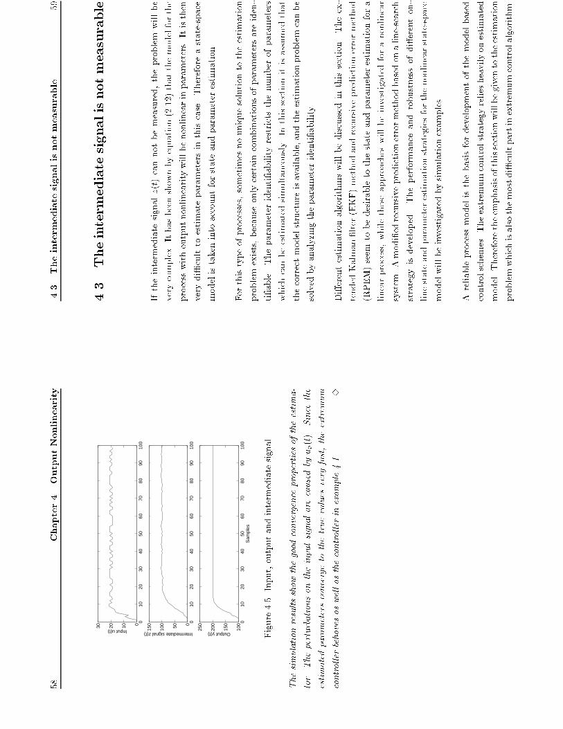
58

Chapter4.OutputNonlinearity

010

2030

4050

6070

8090

100

0102030 Input u(t)

010

2030

4050

6070

8090

100

050100

150

Intermediate signal z(t)

010

2030

4050

6070

8090

100

100

150

200

250

Output y(t)

Sam

ples

Figure4.5.Input,outputandintermediatesignal

Thesimulationresultsshowthegoodconvergencepropertiesoftheestima-

tor.Theperturbationsontheinputsignalarecausedbyup(t).Sincethe

estimatedparametersconvergetothetruevaluesveryfast,theextremum

controllerbehavesaswellasthecontrollerinexample4.1.

3

4.3

Theintermediatesignalisnotmeasurable

59

4.3

Theintermediatesignalisnotmeasurable

Iftheintermediatesignalz(t)cannotbemeasured,theproblemwillbe

verycomplex.Ithasbeenshownbyequation(2.12)thatthemodelforthe

processwithoutputnonlinearitywillbenonlinearinparameters.Itisthen

verydi�culttoestimateparametersinthiscase.Thereforeastate-space

modelistakenintoaccountforstateandparameterestimation.

Forthistypeofprocesses,sometimesnouniquesolutiontotheestimation

problemexists,becauseonlycertaincombinationsofparametersareiden-

ti�able.Theparameteridenti�abilityrestrictsthenumberofparameters

whichcanbeestimatedsimultaneously.Inthissectionitisassumedthat

thecorrectmodelstructureisavailable,andtheestimationproblemcanbe

solvedbyanalyzingtheparameteridenti�ability.

Di�erentestimationalgorithmswillbediscussedinthissection.Theex-

tendedKalman�lter(EKF)methodandrecursivepredictionerrormethod

(RPEM)seemtobedesirabletothestateandparameterestimationfora

linearprocess,whiletheseapproacheswillbeinvestigatedforanonlinear

system.Amodi�edrecursivepredictionerrormethodbasedonaline-search

strategyisdeveloped.Theperformanceandrobustnessofdi�erenton-

linestateandparameterestimationstrategiesforthenonlinearstate-space

modelwillbeinvestigatedbysimulationexamples.

Areliableprocessmodelisthebasisfordevelopmentofthemodelbased

controlschemes.Theextremumcontrolstrategyreliesheavilyonestimated

model.Thereforetheemphasisofthissectionwillbegiventotheestimation

problemwhichisalsothemostdi�cultpartinextremumcontrolalgorithm.

60

Chapter4.OutputNonlinearity

4.3.1

TheEKFasaparameterestimatorforthenon-

linearsystem

Thealgorithm

TheextendedKalman�lter(EKF)isanapproximate�lterfornonlinear

systems,basedon�rst-orderlinearization.Itsuseforjointparameterand

stateestimationproblem

forlinearsystemswithunknownparametersis

wellknownandwidelyspread.Thealgorithmandconvergenceanalysis

havebeengivenbyLjungin[Ljung79b],whichissummarizedinAppendix

C.

Thejointstateandparameterestimationcanofcoursebeunderstoodas

astateestimationproblemforanonlinearsystem,wheretheunknownpa-

rametersarethoughtofrandomvariables.Thereforeitisafairlynatural

thingtoincludetheunknownparametersinthestatevector.Basedon

observationsofotherrandomvariablesthatarecorrelatedwithparameters,

wemayinferinformationabouttheirvalues.Sincetheunobservedstate

vectorisassumedtobecorrelatedwiththeoutputofthesystem,thevalue

ofthestatevectorcanbeestimatedbasedontheobservationofoutput.

InthissectiontheperformanceoftheEKFalgorithmusedasajointstate

andparameterestimationmethodforanonlinearsystem

ratherthana

linearsystemwillbeinvestigated.

Firstofallwesupposethatthesystem

dynamicscanbedescribedbya

generalnonlinearstate-spacemodelgiveninequation(2.31)-(2.32)in

termsofaparametervector�whichisconsideredtobearandomvectorwith

4.3

Theintermediatesignalisnotmeasurable

61

acertainpriordistribution.MatricesQw(�)andQe(�)innonlinearmodel

(2.31)-(2.32)areassumedtobeindependentof�,butarechosen�xed

insomeadhocwayintheremainderofthissection.Thiscorrespondsto

thefactthatnoisecharacteristicsareindependentofthestate,i.e.,w�(t)=

w(t),e �(t)=e(t)andQw(�)=Qw,Qe(�)=Qe.Itisalsoassumedthat

thenoisesequencesfw�(t)gandfe�(t)gareuncorrelated,Qwe(�)=0.

TheEKFapproachgiveninAppendixCforalinearsystemtodetermine

theunknownparametervector�willbemodi�edforanonlinearsystem

(2.31)-(2.32).Theunknownparametervector�innonlinearmodelis

obtainedbyextendingthestatevectorxwiththeparametervector�

x(t)=

x(t)

�(t)

!

(4.19)

thenonlinearstate-spacemodelwillthenbe

x(t+1)

=

f(x(t);u(t))+

w(t)

0

!

y(t)

=

h(x(t))+e(t)

(4.20)

where

f(x(t);u(t))

=

" f(x(t);u(t);�(t))

�(t)

#

h(x(t))

=

h(x(t);�(t))

(4.21)

TheEKFalgorithmforthisjointstateandparametermodelis

^x(t+1)=f(^x(t);u(t))+Kx(t)[y(t)�h(^x(t))]

(4.22)

^x(0)=^x0

K(t)

=

[F(^x(t);u(t))� P(t)HT(^x(t))]

�[H(^x(t))� P(t)HT(^x(t))+Qe]�1

(4.23)

62

Chapter4.OutputNonlinearity

� P(t+1)

=

F(^x(t);u(t))� P(t)FT(^x(t);u(t))+� Qw

�K(t)[H(^x(t))� P(t)HT(^x(t))+Qe]KT(t)

(4.24)

� P(0)=

� P0

where

F(^x(t);u(t))

=

@ @xf(x;u)� � � x=^x(t)

=

" A(^ �(t))

M(^ �(t);^x(t);u(t))

0

I

#

(4.25)

H(^x(t))

=

@ @xh(x)� � � x=^x(t)

=

[C(^ �(t))D(^ �(t);^x(t))]

(4.26)

� Qw

=

" Qw

0

0

0#

(4.27)

^x0

=

" ^x0 ^ � 0

#

� P0

=

�(^ �0)

0

0

�0

!

(4.28)

and

A(^x(t);^ �(t))=

@ @x

f(x(t);u(t);^ �(t))� � � � x=^x

(t)

(anxjnx

matrix)

M(^x(t);u(t);^ �(t))=

@ @�

f(^x(t);u(t);�(t))� � � � �=^ �

(t)

(anxjn�

matrix)

C(^x(t);^ �(t))=

@ @x

h(x(t);^ �(t))� � � � x=^x

(t)

(anyjnx

matrix)

(4.29)

D(^x(t);^ �(t))=

@ @�

h(^x(t);�(t))� � � � �=^ �

(t)

(anyjn�

matrix)

4.3

Theintermediatesignalisnotmeasurable

63

ThealgorithmcanbeseparatedintotwostepsifwewritematrixKx(t)and

� Pas

Kx(t)=

" Kx(t)

K�(t)

#

� P(t)=

" P1(t)

P2(t)

PT 2(t)

P3(t)

#

Parameterscanthenbecomputedinaparameterestimator,andthere-

sultingmodelisusedinastateestimator.Thealgorithmissummarizedas

follows

^x(t+1)=f(^x(t);u(t);^ �(t))+Kx(t)[y(t)�h(^x(t);^ �(t))]

^x(0)=^x0

^ �(t+1)=^ �(t)+K�(t)[y(t)�h(^x(t);^ �(t))]

^ �(0)=^ � 0

Kx(t)=[AtP1(t)CT t

+MtP

T 2(t)CT t

+AtP2(t)DT t

+MtP3(t)DT t]S�1t

K�(t)=[PT 2(t)CT t

+P3(t)DT t]S�1t

(4.30)

St=CtP1(t)CT t

+CtP2(t)DT t

+DtPT 2(t)CT t

+DtP3(t)DT t

+Qe

P1(t+1)=AtP1(t)AT t+AtP2(t)MT t

+MtPT 2(t)AT t+MtP3(t)MT t

�Kx(t)StKT x(t)+Qw

P1(0)=�(^ �0)

P2(t+1)=AtP2(t)+MtP3(t)�Kx(t)StKT �(t)

P2(0)=0

P3(t+1)=P3(t)�K�(t)StKT �(t)

P3(0)=�0

64

Chapter4.OutputNonlinearity

and^ � 0,^x0and�0representsomeaprioriinformationaboutparameter

vector�andstatevectorx.

Inthealgorithm

At=A(^x(t);^ �(t))

Ct=C(^x(t);^ �(t))

Dt=D(^x(t);^ �(t))

(4.31)

Mt=M(^x(t);u(t);^ �(t))

Itisawell-knownfactthatthebehavioroftheEKFasjointstateandpa-

rameterestimatorissensitivetothestatisticsassumptions,anddivergence

mayoccuriftheinitialstateandparameterestimatesarenotsu�ciently

good.Thealgorithmmayconvergeonlyiftheassumptionaboutthenoise

structureofthemodelareinaccordancewiththoseofthetruesystem.

Otherwisetheestimateswillbebiased.Ljungin

[Ljung79b]hasproved

thatthelackofcouplingbetweenstateupdatematrixKx(t)andparameter

vector�,i.e.,[dKx=d�]�(t)=0isassumedinthealgorithm,willleadto

divergenceoftheestimation.

Casestudy

AsimulationexampleisgiventotesttheperformanceoftheEKFalgorithm.

Thepurposeoftheexampleisto�ndtheextremumpointoftheprocesswith

outputnonlinearityandkeeptheoutputatthispoint.Sincethedynamics

oftheprocessisunknown,andintermediatesignalisnotmeasurable,the

EKFalgorithmwillbeusedasajointstateandparameterestimator.Inthe

4.3

Theintermediatesignalisnotmeasurable

65

examplethemodelstructureoftheprocessisassumedtobeinaccordance

withthetrueone.

Example4.3Forthemodelinexample4.1insection4.2,itisassumed

thatthedynamicsoflinearpartisknown,whiletheparametersinthemodel

ofnonlinearparthavetobeestimated.Itisalsoassumedthattheinterme-

diatesignalz(t)isnotabletomeasure.

Letthemodel(4.15)-(4.16)begivenbyastate-spaceform

x(t+1)=ax(t)+bu(t)+w(t)

y(t)=h(�;x(t))+e(t)

(4.32)

and

h(�;x(t))=g 0+g 1x(t)+g 2x2(t)

withparametersa=0:8,b=1,g 0=100,g 1=2andg 2=�0:01.w(t)

ande(t)areuncorrelatedzeromeanwhitenoisewithvariance�2 w

=0:22

and�2 e=0:012respectively.Thevariancesofmeasurementnoiseandthe

processnoiseinthemodelarechoseninaccordancewiththoseofthetrue

system.

Onlytheparametersinoutputequationhavetobeestimated,theparameter

vector�is

�=[g0;g 1;g 2]T

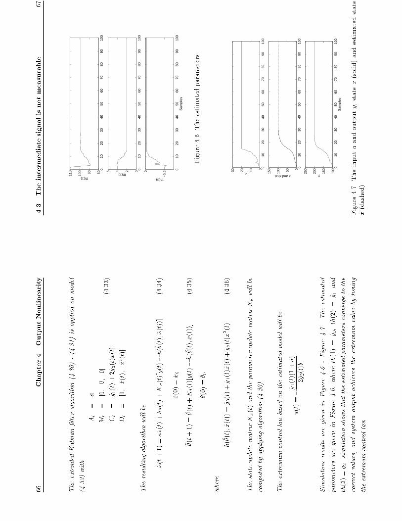
66

Chapter4.OutputNonlinearity

TheextendedKalman�lteralgorithm(4.30)-(4.31)isappliedonmodel

(4.32)with

At

=

a

Mt

=

[0;0;0]

Ct

=

^g 1(t)+2^g 2(t)^x(t)

Dt

=

[1;^x(t);^x2(t)]

(4.33)

Theresultingalgorithmwillbe

^x(t+1)=a^x(t)+bu(t)+Kx(t)[y(t)�h(^ �(t);^x(t))]

(4.34)

^x(0)=^x0

^ �(t+1)=^ �(t)+K�(t)[y(t)�h(^ �(t);^x(t))]

(4.35)

^ �(0)=^ � 0

where

h(^ �(t);^x(t))=^g 0(t)+^g 1(t)^x(t)+^g 2(t)^x2(t)

(4.36)

ThestateupdatematrixKx(t)andtheparameterupdatematrixK�willbe

computedbyapplyingalgorithm(4.30).

Theextremumcontrollawbasedontheestimatedmodelwillbe

u(t)=�

^g 1(t)(1+a)

2^g 2(t)b

SimulationresultsaregiveninFigure4.6-Figure4.7.Theestimated

parametersaregiveninFigure4.6,whereth(1)=

^g 0,th(2)=

^g 1and

th(3)=^g 2.simulationshowsthattheestimatedparametersconvergetothe

correctvalues,andsystem

outputachievestheextremum

valuebytuning

theextremumcontrollaw.

4.3

Theintermediatesignalisnotmeasurable

67

010

2030

4050

6070

8090

100

8090100

110

th(1)

010

2030

4050

6070

8090

100

0246 th(2)

010

2030

4050

6070

8090

100

−0.

20

th(3)

Sam

ples

Figure4.6.Theestimatedparameters.

010

2030

4050

6070

8090

100

0102030 u

010

2030

4050

6070

8090

100

050100

150

x and xhat

010

2030

4050

6070

8090

100

100

150

200

250

y

Sam

ples

Figure4.7.Theinputuandoutputy,statex(solid)andestimatedstate

^x(dashed).

68

Chapter4.OutputNonlinearity

Theconvergenceofestimationrequirestheconditionthattheinitialvalues

oftheestimatedparametersshouldbeinsideaconvergencearea(nottoo

farfromthetruevalues),andtheinitialvariancematrixoftheestimated

parametersP3(0)inthealgorithm(4.30)cannotbeassumedtoolargein

ordertoboundtheestimatedparametersat�rstseveralsteps,otherwise

theeigenvaluesofmatrixAt�KxCtwillbefarfromtheunitcircle.This

willcausethedivergenceoftheprocess.Goodinitialstateestimatesare

alsoimportantfortheconvergenceproperties.Theincreasednumberof

parameterstobeestimatedfrequentlyresultsinreducedrobustness.

TheEKFasajointstateandparameterestimatorworkswellwhenagood

modelandreasonableparameterestimatesareavailable,thenonlinearityis

weakandnoiseassumptionsareclosetothetruth.

Asitisstatedin

[Ljung79b],thereasonforthedivergenceoftheEKF

asajointparameterandstateestimationforalinearsystem

isthatthe

e�ectontheKalmangainKx

ofachangein�isnottakencareof.For

caseswherethesteady-stateKalmangaindoesnotdependon�,wewill

havegoodconvergenceproperties.Theestimationproblemissigni�cantly

simpli�edifthe�ltergainsensitivitiestotheparametersareneglected,i.e.,

[dKx=d�]�(t)=0.Theestimationproblemcanthenbeseparatedintotwo

estimators.Theparameterswerecomputedinaparameterestimator,and

resultingmodelisusedinastateestimator.

Foranonlinearsystemthealgorithmismoresensitive.Accordingtoequa-

tions(C.37)-(C.39)inAppendixC,thesteadystateKalmangainmatrix

ofalinearsystem

isindependentofstatevariableswhichappearonlyin

MtandDtmatrices.However,foranonlinearsystem,sincethestateup-

datematrixKx(t)inthealgorithm(4.30)iscalculatedbyusingalinearized

4.3

Theintermediatesignalisnotmeasurable

69

modelwhichisactuallyanapproximationofthetruemodel.Parametersof

thelinearizedmodeldependnotonlyontheestimatedparametersbutalso

ontheestimatedstates(e.g.,matrixCtin(4.33)).Thereforethesteady-

stateKalmangainmatrixofanonlinearsystemdependsonestimatedstate

vector.Thiswillcausethealgorithmmoresensitive.Themodelparam-

eterestimateswillbepoorwhentheestimatedstatesarenotclosetothe

truevalues.Thepoormodelparameterestimateswillmakethealgorithm

todiverge,since[dKx=d�]�(t)isnotaccountedforinthealgorithm,and

sensitivitymatrix (t)=�d=d��(t)hasatendencytobeincorrect.

3

4.3.2

TheRPEM

appliedtotheinnovationsmodel

Itisofcourseunrealistictoassumethatthenoisestructureisknown,while

thedynamicsareunknown.Therefore,ifthenoisecharacteristicofthe

modelischosenadhoc,thenthesystemparameterestimateswillingeneral

bebiased[Ljung79b].LjungsuggestedaNewton-typestochasticgradient

algorithminhisreport.

ArecursiveGauss-Newtonalgorithmwhichminimizespredictionerrorcri-

terionwillleadtoarecursivepredictionerrormethod(RPEM).TheRPEM

istakeintoconsideration,sinceLjunghasprovedthattheRPEMappliedto

thejointstateandparameterestimationprobleminastationaryinnovations

state-spacemodelhasbetterconvergencepropertiesthanthecorrespond-

ingEKF.ThecouplingbetweenupdatestatematrixKx(t)andparameter

vector�isincludedintheRPEMalgorithm.

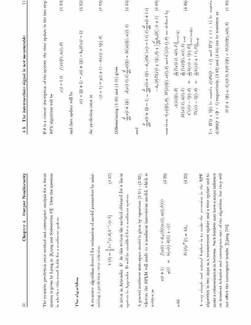
70

Chapter4.OutputNonlinearity

Therecursivepredictionerrormethodandconvergenceanalysisforalinear

systemisgivenbyLjungin[LjungandS�oderstr�om83].Thenthequestion

iswhetherthisresultholdsforanonlinearsystem.

Thealgorithm

Arecursivealgorithmderivedforestimationofmodelparametersbymini-

mizingapredictionerrorcriterion

V(�)=

1 2E�T(t;�)��1�(t;�)

(4.37)

isgiveninAppendix

D.Inthissectionthemethodobtainedforalinear

systeminAppendixDwillbemodi�edforanonlinearsystem.

Ageneralnonlinearstate-spacemodelisgivenbyequations(2.31)-(2.32),

whereastheRPEM

willapplytoanonlinearinnovationsmodel,whichis

writtenas

x(t+1)

=

f(x(t)+Kx(�(t))�(t);u(t);�(t))

y(t)

=

h(x(t);�(t))+�(t)

(4.38)

with

E�(t)�T(t)=�� ts

(4.39)

AverysimpleandnaturalfeatheristomaketherecursionintheRPE

algorithmintwostepsasameasurementupdateandatimeupdateandto

makearelinearizationinbetween.Suchfeathersmayhaveamajorin uence

ontransientbehaviorandconvergencerateofthealgorithm,buttheywill

note�ecttheconvergenceresults[Ljung79b].

4.3

Theintermediatesignalisnotmeasurable

71

If�isacorrectdescriptionofthesystem,thetimeupdateinthetwostep

RPEalgorithmwillbe

^x(t+1jt)=f(^x(tjt);u(t);�)

(4.40)

anddateupdatewillbe

^x(t+1jt+1)=^x(t+1jt)+kx(�)�(t+1)

(4.41)

thepredictionerroris �(

t+1)=y(t+1)�h(^x(t+1jt);�)

(4.42)

Di�erentiating(4.40)and(4.41)gives

d d�

^x(t+1jt)=A(^x(tjt);�)

d d�

^x(tjt)+M(^x(tjt);u(t);�)

(4.43)

and

d d�

^x(t+1jt+1)=

d d�

^x(t+1jt)�kx(�)C(^x(t+1jt);�)

d d�

^x(t+1jt)

�kx(�)D(^x(t+1jt);�)+[

d d�

kx(�)]�(t+1)

(4.44)

matricesA(^x(tjt);�),M(^x(tjt);u(t);�)andC(^x(tjt);�)arede�nedby

A(^x(tjt);�)

=

@ @xf(x(tjt);u(t);�)

� � x=^x(tjt)

M(^x(tjt);u(t);�)

=

@ @�f(^x(tjt);u(t);�)

� � �=�

C(^x(t+1jt);�)

=

@ @xh(x(t+1jt);�)

� � x=^x(t+1jt)

D(^x(t+1jt);�)

=

@ @�h(^x(t+1jt);�)

� � �=�

(4.45)

LetW(t+1jt)bematrixd=d�^x(t+1jt)andW(t+1jt+1)bematrix

d=d�^x(t+1jt+1)respectively,(4.43)and(4.44)canberewrittenas

W(t+1jt)=A(^x(tjt);�)W(tjt)+M(^x(tjt);u(t);�)

(4.46)

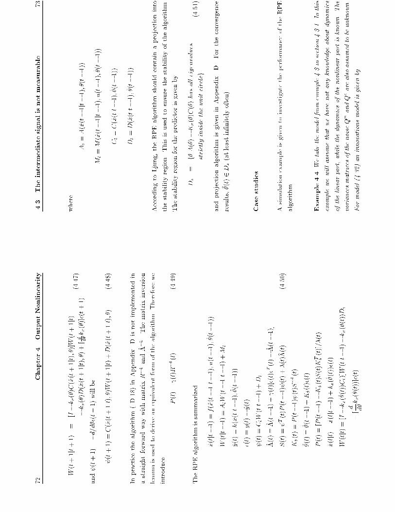
72

Chapter4.OutputNonlinearity

W(t+1jt+1)

=

[I�kx(�)C(^x(t+1jt);�)]W(t+1jt)

�kx(�)D(^x(t+1jt);�)+[d d�kx(�)]�(t+1)

(4.47)

and (t+1)=�d=d��(t+1)willbe

(t+1)=C(^x(t+1jt);�)W(t+1jt)+D(^x(t+1jt);�)

(4.48)

Inpracticethealgorithm(D.18)inAppendix

Disnotimplementedin

astraightforwardwaywithmatrixR�1and^ ��1.Thematrixinversion

lemmaisusedtoderiveanequivalentformofthealgorithm.Thereforewe

introduce

P(t)= (t)R�1(t)

(4.49)

TheRPEalgorithmissummarized

^x(tjt�1)=f(^x(t�1jt�1);u(t�1);^ �(t�1))

W(tjt�1)=AtW(t�1jt�1)+Mt

^y(t)=h(^x(tjt�1);^ �(t�1))

�(t)=y(t)�^y(t)

(t)=CtW(tjt�1)+Dt

^ �(t)=^ �(t�1)+ (t)[�(t)�T(t)�^ �(t�1)]

S(t)= T(t)P(t�1) (t)+�(t)^ �(t)

(4.50)

K�(t)=P(t�1) (t)S�1(t)

^ �(t)=^ �(t�1)+K�(t)�(t)

P(t)=[P(t�1)�K�(t)S(t)KT �(t)]=�(t)

^x(tjt)=^x(tjt�1)+kx(^ �(t))�(t)

W(tjt)=[I�kx(^ �(t))Ct)]W(tjt�1)�kx(^ �(t))Dt

+[

d d�

kx(^ �(t))]�(t)

4.3

Theintermediatesignalisnotmeasurable

73

where

At=A(^x(t�1jt�1);^ �(t�1))

Mt=M(^x(t�1jt�1);u(t�1);^ �(t�1))

Ct=C(^x(tjt�1);^ �(t�1))

Dt=D(^x(tjt�1);^ �(t�1))

AccordingtoLjung,theRPEalgorithmshouldcontainaprojectioninto

thestabilityregion.Thisisusedtoensurethestabilityofthealgorithm.

Thestabilityregionforthepredictorisgivenby

Ds

=

f�jA(�)�Kx(�)C(�)hasalleigenvalues

strictlyinsidetheunitcircleg

(4.51)

andprojectionalgorithmisgiveninAppendix

D.Fortheconvergence

results,^ �(t)2Ds(atleastin�nitelyoften).

Casestudies

AsimulationexampleisgiventoinvestigatetheperformanceoftheRPE

algorithm.

Example4.4Wetakethemodelfromexample4.3insection4.3.1.Inthis

examplewewillassumethatwehavenotanyknowledgeaboutdynamics

ofthelinearpart,whilethedynamicsofthenonlinearpartisknown.The

variancesmatricesofthenoiseQw

andQearealsoassumedtobeunknown.

Formodel(4.32)aninnovationsmodelisgivenby

74

Chapter4.OutputNonlinearity

x(t+1)

=

ax(t)+bu(t)+Kx�(t)

y(t)

=

h(t;x(t))+e(t)

(4.52)

where

h(t;x(t))=g 0+g 1x(t)+g 2x2(t)

Theestimatedparametervector�willbe

�=[a;b;kx]T

ThetwostepRPEM

(4.50)willbeimplementedfortheinnovationsmodel

with

At=^a(t�1)

Ct=g 1+2g 2^x(tjt�1)

Dt=[0;0;0]

Mt=[^x(t�1jt�1);u(t�1);0]

Theextremumcontrollawbasedontheestimatedmodelis

u(t)=�

g 1(1+^a)

2g 2^ b

ThesimulationresultsaregiveninFigure4.8-4.9.Theestimatedparam-

etersareshowninFigure4.8,whereth(1)=^a,th(2)=^ bandth(3)=

^ kx.

Thetruevaluesofparametersaandbaregivenbythedashedlineinthe

�gure.Theestimatesconvergetothecorrectvaluesveryfast.Theinput,

outputandstatearegiveninFigure4.9.Theoutputachievestheextremum

valuequickly.Thealgorithmshowsasatisfactoryperformance.

4.3

Theintermediatesignalisnotmeasurable

75

010

2030

4050

6070

8090

100

0.6

0.8

th(1)

010

2030

4050

6070

8090

100

1th(2)

010

2030

4050

6070

8090

100

1.1

1.151.

2

th(3)

Sam

ples

Figure4.8.Theestimatedparameters.

010

2030

4050

6070

8090

100

0204060 u

010

2030

4050

6070

8090

100

050100

150

x and xhat

010

2030

4050

6070

8090

100

0

100

200

300

y

Sam

ples

Figure4.9.Theinputuandoutputy,statex(solid)andestimatedstate

^x(dashed)

76

Chapter4.OutputNonlinearity

SimulationexperiencesshowthattheRPEM

algorithmintwostepsgives

abettertransientresponsethantheoriginalRPEM.Thisisbecausethe

estimatedsensitivitymatrix iscountedinparameterestimatesatthe�rst

step.Thesimulationwillnotbeheavilyin uencedbytheassumptionof

initialKx.However,thereisalittlebiasintheestimatedparameters.

Thebadassumptionsoftheinitialparameterestimatesandstateestimates

willmakethesimulationdiverge,whichmeansthatgoodassumptionsof

initialvaluesarerequiredforasuccessfulsimulation.

Intheinnovationsmodel(4.38),thesteady-stateKalmangain,ratherthan

thecovariancematrices,isparameterized.Thissteady-stateKalmangainis

usedintheRPEalgorithmallthetimeasatime-invariantpredictor.This

actuallyimpliesthatthealgorithminprincipleisbasedontheassumption

thatthestateupdatematrixKxisconstant,oratleastasymptoticallycon-

stant.Fornonlinearsystems,Kx

willvaryrapidlyastheinputandthe

operationalpointchange.ThenifKxispoor,thesubsequentW(t+1)and

(t+1)willhaveatendencytobeincorrect.Theestimatorwillbebiased

ordiverge.

3

4.3.3

Themodi�edrecursivepredictionerrormethod

Amodi�edrecursivepredictionerrormethodbasedonalinesearchstrategy

wassuggestedbyLjungquistin

[LjungquistandBalchen93].TheLine

searchtechniquesarewidelyusedtosolveoptimizationproblems.Inthis

algorithmthelinesearchperformsinthecomputedsearchdirectionto�nd

anoptimalstepsizeduringeachiteration.Duetothenonlinearitiesaline

4.3

Theintermediatesignalisnotmeasurable

77

searchstrategyisusedtoavoiddivergencewhenthesearchdirectionis

pro�table.

Linesearchtechnique

AlinesearchmethodusedtosolveoptimizationproblemhasbeeninAp-

pendixA.6.Whenthesearchdirectionhasbeendeterminedforparameter

estimator

^ �(t)=^ �(t�1)+�(t)K�(t)�(t)

(4.53)

wehavetodecidehowlongthestepinthisdirectionshouldbe.

Theoptimalparameterupdatingstepsizewhichisfoundbyperforming

thelinesearchapproachcanbecomputedbyminimizingtheone-sample

criterion

Vj(t)=� j(t)T^ ��1(t)�j(t)+�^ � j(t)TP�1(t)�^ � j(t)

(4.54)

where

�^ � j(t)=^ � j(t)�^ �(t�1)

(4.55)

�(t)andP(t)arepositivede�nitematrices.

Duringthelinesearch,anewparametervectoriscomputedaccordingto

^ � j(t)=^ �(t�1)+�j(t)K�(t)�(t)

(4.56)

where�j(t)istheupdatestepsize.Oncethesearchdirectionateachdiscrete

sampletimeisdetermined,thevalueofcriterion(4.54)isafunctionofthe

stepsize�alone.Thentheoptimalstepsizecanbeobtainedbyminimizing

thecriterion

�0(t)=min �V(�;t)

(4.57)

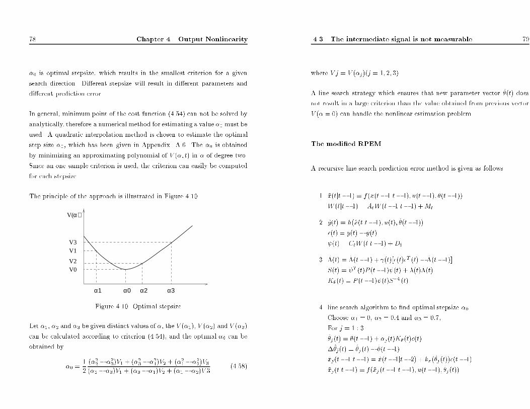
78 Chapter 4. Output Nonlinearity

�0 is optimal stepsize, which results in the smallest criterion for a given

search direction. Di�erent stepsize will result in di�erent parameters and

di�erent prediction error.

In general, minimum point of the cost function (4.54) can not be solved by

analytically, therefore a numerical method for estimating a value �0 must be

used. A quadratic interpolation method is chosen to estimate the optimal

step size �0, which has been given in Appendix A.6. The �0 is obtained

by minimizing an approximating polynomial of V (�; t) in � of degree two.

Since an one sample criterion is used, the criterion can easily be computed

for each stepsize.

The principle of the approach is illustrated in Figure 4.10.

V(

V3

α

α1 α0 α2 α3

)

V1

V2V0

Figure 4.10. Optimal stepsize

Let �1, �2 and �3 be given distinct values of �, the V (�1), V (�2) and V (�3)

can be calculated according to criterion (4.54), and the optimal �0 can be

obtained by�0 =

12

(�22 � �23)V1 + (�23 � �21)V2 + (�21 � �22)V3

(�2 � �3)V1 + (�3 � �1)V2 + (�1 � �2)V 3

(4.58)

4.3 The intermediate signal is not measurable 79

where V j = V (�j)(j = 1; 2; 3).

A line search strategy which ensures that new parameter vector ^�(t) does

not result in a large criterion than the value obtained from previous vector

V (� = 0) can handle the nonlinear estimation problem.

The modi�ed RPEM

A recursive line search prediction error method is given as follows.

1. ^x(tjt� 1) = f(^x(t� 1jt� 1); u(t� 1); ^�(t � 1))

W (tjt� 1) = AtW (t� 1jt� 1) +Mt

2. ^y(t) = h(^x(tjt� 1); u(t); ^�(t� 1))

�(t) = y(t) � ^y(t)

(t) = CtW (tjt� 1) +Dt

3. ^�(t) = ^�(t� 1) + (t)[�(t)�T (t) � ^�(t� 1)]

S(t) = T (t)P (t� 1) (t) + �(t)^�(t)

K�(t) = P (t� 1) (t)S�1(t)

4. line search algorithm to �nd optimal stepsize �0.

Choose �1 = 0, �2 = 0:4 and �3 = 0:7,

For j = 1 : 3

^�j(t) = ^�(t� 1) + �j(t)K�(t)�(t)

�^�j(t) = ^�j(t)� ^�(t � 1)

^xj(t� 1jt� 1) = ^x(t� 1jt� 2) + kx(^�j(t))�(t� 1)

^xj(tjt� 1) = f(^xj (t� 1jt� 1); u(t� 1); ^�j(t))

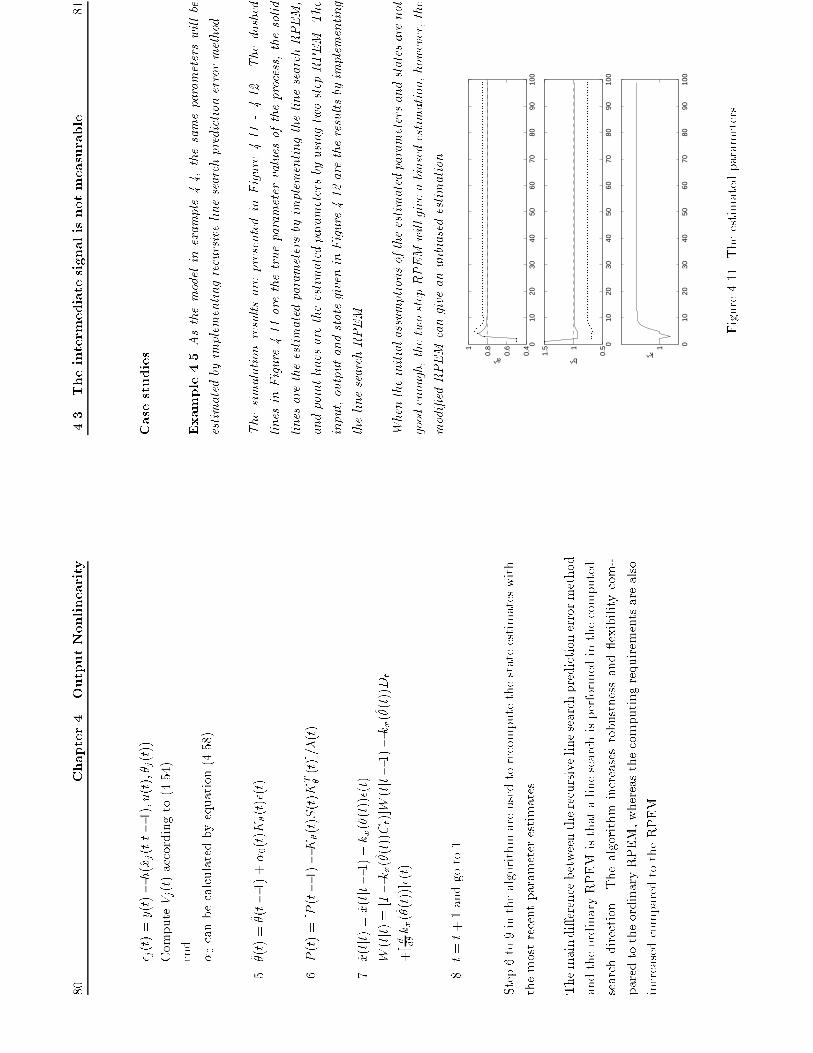
80

Chapter4.OutputNonlinearity

� j(t)=y(t)�h(^xj(tjt�1);u(t);^ � j(t))

ComputeVj(t)accordingto(4.54)

end

�0canbecalculatedbyequation(4.58).

5.^ �(t)=^ �(t�1)+�0(t)K�(t)�(t)

6.P(t)=[P(t�1)�K�(t)S(t)KT �(t)]=�(t)

7.^x(tjt)=^x(tjt�1)+kx(^ �(t))�(t)

W(tjt)=[I�kx(^ �(t))Ct)]W(tjt�1)�kx(^ �(t))Dt

+[d d�kx(^ �(t))]�(t)

8.t=t+1andgoto1.

Step6to9inthealgorithmareusedtorecomputethestateestimateswith

themostrecentparameterestimates.

Themaindi�erencebetweentherecursivelinesearchpredictionerrormethod

andtheordinaryRPEMisthatalinesearchisperformedinthecomputed

searchdirection.Thealgorithmincreasesrobustnessand exibilitycom-

paredtotheordinaryRPEM,whereasthecomputingrequirementsarealso

increasedcomparedtotheRPEM.

4.3

Theintermediatesignalisnotmeasurable

81

Casestudies

Example4.5Asthemodelinexample4.4,thesameparameterswillbe

estimatedbyimplementingrecursivelinesearchpredictionerrormethod.

ThesimulationresultsarepresentedinFigure4.11-4.12.Thedashed

linesinFigure4.11arethetrueparametervaluesoftheprocess,thesolid

linesaretheestimatedparametersbyimplementingthelinesearchRPEM,

andpointlinesaretheestimatedparametersbyusingtwostepRPEM.The

input,outputandstategiveninFigure4.12aretheresultsbyimplementing

thelinesearchRPEM.

Whentheinitialassumptionsoftheestimatedparametersandstatesarenot

goodenough,thetwostepRPEMwillgiveabiasedestimation,however,the

modi�edRPEM

cangiveanunbiasedestimation.

010

2030

4050

6070

8090

100

0.4

0.6

0.81

a^

010

2030

4050

6070

8090

100

0.51

1.5

b^0

1020

3040

5060

7080

9010

0

1k^

Figure4.11.Theestimatedparameters.

82

Chapter4.OutputNonlinearity

010

2030

4050

6070

8090

100

050100

u

010

2030

4050

6070

8090

100

050100

150

x and xhat

Sam

ples

010

2030

4050

6070

8090

100

0

100

200

300

y

Figure4.12.Theinputandoutput

Thesimulationindicatesthatthemodi�edRPEM

performsbetterthanthe

originalRPEM.Therobustnessofthemodi�edalgorithmishigher,since

toolongandtooshortupdatingstepsduringtransientsareavoided.But

themodi�edRPEM

willincreasethecomplexityandcomputationalcosts.

Anywaytheexampleindicatesthattherecursivelinesearchpredictionerror

methodispreferableforanonlinearsystemwithnonlinearityatoutput.3

4.4

Summary

Whentheintermediatesignalbetweenlinearpartandnonlinearpartof

thenonlinearmodelismeasurable,theproblem

willbesimpli�ed.The

identi�cationcanthenbeimplementedforlinearpartandnonlinearpart

4.4

Summary

83

separately.Inthiscasetheonlydi�erencebetweentheoutputnonlinearity

andinputnonlinearityisthatinputfortheprocesswithoutputnonlinearity

isnotdetermineddirectlybutthoughthelineardynamics.

Whentheintermediatesignalbetweenlinearpartandnonlinearpartisnot

measurable,theparameterestimationbecomesverycomplex.Sincethe

extremumcontrollawreliesheavilyontheestimatedmodel,theestimation

problemisthenthekeypointofimplementationofthecontrollaw.

Someoftheconclusionsreachedinthischapterarebasedonwell-established

theory,othersarebasedonsimulationstudies,sincenonlinearsystemsare

di�culttodealwithstrictlytheoretically.Clearly,simulationstudiesdo

notprovethatonestrategyisingeneralbetterthananother,buttheycan

showthatoneapproachispreferabletoanotherforaclassofproblems.

Forthesystemwithknownnoisestructureandweaknonlinearity,theEKF

asajointstateandparameterestimatorworkswell.However,forthesystem

withunknowndynamicsandunknownnoisestructure,themethodmaygive

biasedestimates,anditdoesnotseldomdivergeiftheinitialestimatesare

notsu�cientlygood.Thereasonfordivergencecanbeinterpretedthatthe

e�ectontheKalmangainKx

ofachangein�isnottakenintoaccount.

ThislackofcouplingbetweenKx(t)and�inthealgorithmmayleadto

divergenceoftheestimates.

Example

4.3simulatesofthebehaviouroftheEKFestimatorandex-

tremumcontrolleronanonlinearsystemwithknownnoisevariances.The

EKFalgorithmandextremumcontrollawworkwellinthiscase.However,

theEKFalgorithmasastateandparameterestimatorismoresensitive

whenitisappliedtoanonlinearsystemratherthanalinearsystem.For

84

Chapter4.OutputNonlinearity

anonlinearsystem,thestateupdatematrixKx(t)inthealgorithmiscal-

culatedbyusingalinearizedmodelwhichisactuallyanapproximationof

thetruemodel.Theapproximationwillmakethealgorithmmoresensitive.

Thepoormodelparameterestimateswillmakethealgorithmtodiverge,

since[dKx=d�]�(t)isnotaccountedforinthealgorithm.

Inordertoimprovetheglobalconvergenceresults,theRPEM

isapplied

foraninnovationsmodel.The[d=d�� Kx(�)]�(t)isincludedintheRPEalgo-

rithm.Inexample4.4atwostepRPEalgorithmisappliedtoaninnovations

model.Theestimatorandregulatorworkwelliftheinitialassumption

aboutestimatedparametersandstatesaregoodenough.TheRPEMbased

ontheinnovationsstate-spacemodelmeansthatthealgorithminprinciple

isbasedontheassumptionthatthestateupdatingmatrixKxisconstant,at

leastasymptotically.However,foranonlinearsystemKxwillvaryrapidly

astheinputsandtheoperationalpointchange,atleastwhentheestimation

hasnotconvergedandextremumpointhasnotbeenreached.IfKxispoor,

thesubsequentW(t+1)and (t+1)willhaveatendencytobeincorrect.

Theestimatorwillbebiasedordiverge.

BoththeEKFalgorithmasjointstateandparameterestimationmethod

andtheRPEMcanbesuccessfullyappliedtoanumberofestimationprob-

lems.

Amodi�edRPEalgorithmbasedonline-searchstrategyisdevelopedin

section4.3.3.Inthisalgorithmtheline-searchperformsinthecomputed

searchdirectionto�ndanoptimalstepsizeduringeachiteration.Example

4.5showsthatthemodi�edRPEalgorithm

givesabetterperformance

thantheoriginalRPEalgorithm.Therobustnessofmodi�edalgorithmis

increased,sincetoolongandtooshortstepsareavoided.

Chapter5

Conclusions

Problemsofextremum

controlhavebeenfrequentlystudiedbyagood

numberofauthors.Thereasonmaybethepossibilitytodescribeseveral

interestingpracticalproblems.Thereare,e.g.,industrialprocesseswhere

theobjectofcontrolistomaximizesomephysicalvariablesuchasanef-

�ciency.Ifthereexistssomeoptimalvalueforthecontrolvariablegiving

maximalvaluefortheoutput,thentheproblemisofthistype.

Toperform

adaptiveextremum

controlofnonlinearsystems,itisneces-

sarytomakeassumptionsaboutthestructureoftheprocess.Oneofclass

ofsystemsisobtainedbydividingtheprocessintoanonlinearstaticpart

andlineardynamicpart.Approximationtheoryisusedtoderivedi�erent

typesofseriesexpansionrepresentationsofnonlinearsystems.Therepre-

sentationsincludeVolterra,WienerandUrysonseries.Theycanbeusedto

modeltheprocesseswherethelineardynamicsisfollowedbyanonlinearity.

85

86

Chapter5.Conclusions

TheUrysonseriescanalsoincludethenonlinearityattheinput.Aspe-

cialcaseofUrysonseriesisrepresentedbyHammersteinmodels,whichare

commoncon�gurationsconsideredintheextremumcontrolsystems.The

state-spacemodelscanalsobeemployedtodescribenonlinearprocesses.

Forasystemwithinputnonlinearity,ifthesystemsareunknown,theyhave

tobeidenti�ed.Mostidenti�cationmethodsarebasedontheassumption

thatthemodelislinearinparameters.AHammersteinmodeloftheprocess

withtheinputnonlinearityhasthiskindofproperty.Anon-linerecur-

siveestimationalgorithm,e.g.,therecursiveextendedleastsquares(RELS)

methodisappliedtoidentifytheparametersofthemodel.Theextremum

controllawisderivedbymaximizingorminimizingthestaticresponseof

processoutput,whichwillkeeptheprocessoperatingat,orinthevicin-

ityof,theextremumpointoftheperformancefunctionorprocessoutput

despiteofthein uenceofthedisturbances.Atestperturbationsignalis

necessarytoensuretheparameteridenti�ability,whichhasbeenprovedby

analyzingconvergencepropertiesbyusingODEapproach.Twoexamples

havebeengiventoshowthegoodconvergencepropertiesoftheestimator

andgoodbehaviouroftheextremumcontroller.

Fortheprocesswithoutputnonlinearity,twodi�erentcaseshavebeendis-

cussedaccordingtothattheintermediatesignalcanbemeasuredornot.

Di�erentmodelsandestimationmethodswillbeusedatdi�erentcases.

Iftheintermediatesignalcanbemeasured,theRELSalgorithmisemployed

toestimatetheparametersforlinearpartandnonlinearpartseparately.

Theonlydi�erencebetweentheoutputnonlinearityandinputnonlinearity

isthatitsextremumcontrollawwillnotbedetermineddirectly,butthrough

87

lineardynamics.Thesimulationexamplesshowthegoodbehaviourofthe

estimatorandcontroller.

Iftheintermediatesignalisnotmeasurable,theproblem

becomesquite

complex.Sincetheextremumcontrollawdependheavilyontheestimated

model,theestimationproblembecomesthekeypointoftheadaptiveex-

tremumcontrolalgorithm.

FirstofalltheextendedKalman�lterasajointstateandparameteresti-

matorisconsidered.Astate-spacemodeloftheprocessisemployedinorder

toimplementtheEKFalgorithm.Simulationsforaprocesswithunknown

nonlineardynamicsandknownnoisestructureshowthegoodconvergence

propertiesoftheEKFalgorithmiftheassumedinitialvaluesofstateand

parameterestimatesaregoodenough.

Itisawell-knownfactthatthebehaviorofEKFasjointstateandparam-

eterestimatorissensitivetoaprioristatisticsassumptions,anddivergence

mayoccuriftheinitialstateandparameterestimatesarenotsu�ciently

good.Thealgorithmmayconvergeonlyiftheassumptionsaboutthenoise

structureofthemodelareinaccordancewiththoseofthetruesystem.

Otherwisetheestimateswillbebiased.

However,theEKFalgorithmismoresensitivewhenitisappliedtoanon-

linearsystem.SincethestateupdatematrixKx

iscomputedbasedona

linearizedmodelthatisactuallyanapproximationofthetruemodel.When

thelinearizedmodelisapplied,thesteady-stateKalmandependsalsoon

theestimatedstates.Thealgorithmwillthenbemoresensitive.Thepa-

rameterestimateswillbepoorwhentheestimatedstatesarenotcloseto

thetruevalues.Thepoormodelwillmaketheestimationtodiverge.

88

Chapter5.Conclusions

Ljungsuggestedtherecursivepredictionerrormethod(RPEM)appliedfor

aninnovationsmodeltoimprovetheglobalconvergenceresults.Simulation

indicatesthatestimatorandregulatorworkwelliftheinitialassumptions

aboutestimatedparametersandstatesaregoodenough.TheRPEMbased

ontheinnovationsstate-spacemodelimpliesthatthealgorithminprinciple

isbasedontheassumptionthatthestateupdatingmatrixKxisconstant,

atleastasymptotically.However,forthenonlinearsystemKxwillchange

rapidlyastheinputsandtheoperationalpointchange.

Amodi�edRPEalgorithmbasedonline-searchstrategyispreferablefor

anonlinearsystem.Inthisalgorithmtheline-searchperformsinthecom-

putedsearchdirectionto�ndanoptimalstepsizeduringeachiteration.

Simulationshaveshowedthatthemodi�edRPEalgorithm

hasabetter

performancethantheoriginalRPEalgorithmforanonlinearprocesswith

unknownlineardynamicandnoisestructure.Theincreasedrobustnessof

themodi�edRPEisespeciallyimportantwhentheestimationschemeisto

beappliedonline.

ThesimulationsindicatethatboththeEKFalgorithmasjointstateand

parameterestimationmethodandtheRPEMcanbesuccessfullyappliedto

anumberofestimationproblems.Itisconsequentlyimpossibletostatethat

onealgorithmisalwayspreferabletoanother.Theavailableinformationis

veryimportanttoselectthebestmethodforagivenapplication.

Bibliography

[BambergerandIsermann78]W.BambergerandR.Isermann.Adaptive

On-lineSteady-StateOptimizationofSlowDynamicProcess.Au-

tomatica,Vol.14,pp223-230.1978.

[Blackman1962]P.F.Blackman.Extremum-seekingRegulators.AnExpo-

sitionofAdaptiveControl.PergamonPress,1962.

[Frandsenetal.95]PoulE.Frandsen,KristianJonassonandOleTingle�.

UnconstrainedOptimization.Notestothecourse\Algorithmsfor

non-linearOptimization".InstituteofMathematicalModelling,

TechnicalUniversityofDenmark.1995.

[GoldenandYdstie89]MelindaP.GoldenandB.ErikYdstie.AdaptiveEx-

tremum

ControlUsingApproximateProcessModels.AIChE

Journal,July,1989,Vol.35,No.7.

[GoodwinandSin84]GrahamC.GoodwinandKwaiS.Sin.AdaptiveFil-

teringPredictionandControl.PrenticeHall.1984.

89

90

BIBLIOGRAPHY

[HaberandKeviczky76]R.HaberandL.Keviczky.Identi�cationofNon-

linearDynamicSystems.Proc.of4thIFACSymposiumonIden-

ti�cationandSystemParameterEstimation,Tbilisi,USSR.Sept,

1976.

[JacobsandLangden70]O.L.R.JacobsandS.M.Langdon.AnOptimalEx-

tremalControlSystem.Automatic,Vol.6,pp.297-301.1970.

[Jazwinski70]Andrew

H.Jazwinski.StochasticProcessesandFiltering

Theory.AcademicPress,NewYork.1970.

[KeviczkyandHaber74]L.KeviczkyandR.Haber.AdaptiveDualEx-

tremumControlbyHammersteinModel.Proc.IFACSymposium

onStochasticControl,pp333-341.Budapest,1974.

[Keviczky78]L.K.Keviczky.NonlinearDynamicIdenti�cationofaCe-

mentMilltobeOptimized.Proc.of4thIFACSymposium

on

Identi�cationandSystemParameterEstimation,Tbilisi,USSR.

Sept,1976.

[Keviczkyetal.79]L.Keviczky,I.VajkandJ.Hetth�essy.ASelf-TuningEx-

tremalControllerfortheGeneralizedHammersteinModel.Proc.

IFACSymposiumonIdenti�cation,pp.1147-1151,1979.Darm-

stadt.

[Ljung77]LennartLjung.AnalysisofRecursiveStochasticAlgorithms.

IEEETrans.onAutomaticControl,vol.AC-22,no.4,Aug.1977.

[Ljung79b]LennartLjung.AsymptoticBehavioroftheExtendedKalman

FilterasaParameterEstimatorforLinearSystems.IEEETrans.

onAutomaticControl,vol.AC-24,no.1,Feb.1979.

[LjungandS�oderstr�om83]LennartLjungandTorstenS�oderstr�m.Theory

andPracticeofRecursiveIdenti�cation.TheMITPress,1983.

BIBLIOGRAPHY

91

[Ljung87]LennartLjung.System

Identi�cation:TheoryfortheUser.

Prentice-Hall,Inc.,EnglewoodCli�s,NewJersey.1987.

[Ljungquist90]DagLjungquist.

OnlineEstimationinNonlinearState-spaceModelswithAppli-

cationtoCatalyticCracking.Dr.Ing.Thesis,NorwegianInstitute

ofTechnology.1990.

[LjungquistandBalchen93]DagLjungquistandJensG.Balchen.Recur-

sivePredictionErrorMethodsforOnlineEstimationinNonlinear

State-Spacemodels.Proc.ofthe32ndConf.onDecisionand

Control,Texas.Dec.1993.

[Madsen95]KajMadsen.MinimeringafKvadratsummer,H�fte38.In-

stituteofMathematicalModelling,TechnicalUniversityofDen-

mark.1995.

[MadsenandHolst96]HenrikMadsenandJanHolst.ModellingNon-linear

andNon-stationaryTimeseries.InstituteofMathematicalMod-

elling,TechnicalUniversityofDenmark.1996.

[NavarroandZarrop95]LuisB.NavarroandMartinB.Zarrop.Extremum

ControlApproachtoStochasticControl.Proceedingsof3rdEu-

ropeanControlConference,Rome,Italy,September,1995.

[Poulsen95]NielsK.Poulsen.StokastiskAdaptivRegulering.Instituteof

MathematicalModelling,TechnicalUniversityofDenmark.1995.

[Sternby78]JanSternby.AnalysisofanExtremumControllerforHammer-

steinModels.Report,DepartmentofAutomaticControl,Lund

University,1978.

92

BIBLIOGRAPHY

[Sternby80a]JanSternby.AdaptiveControlofExtremumSystems.Pro-

ceedingsofanInternationalSymposium

onAdaptiveControl,

Bochum,March,1980.

[Sternby80b]JanSternby.ExtremumControlSystems-AnAreaforAdap-

tivecontrol?ProceedingsoftheJointAutomaticControlConfer-

ence,Vol.1,WA2-A.1980.

[S�oderstr�omandStoica89]TorstenS�oderstr�om

andPetreStoica.System

Identi�cation.PrenticeHall,1989.

[Vadstrup85]Pierr�eVadstrup.Ikke-line�reSystemer.InternRapport,Ser-

volaboratoriet,DTH,December,1985.

[Vadstrup88]Pierr�eVadstrup.AdaptivReguleringafIkke-line�reSyste-

mer.Licentiatafhandling,Servolaboratoriet,DTH.Danmark.De-

cember,1988.

[WellsteadandScotson90]P.E.WellsteadandP.G.Scotson.Self-tuningEx-

tremumControl.IEEProceedings,Vol.137,Pt.D,No.3,May,

1990.

[WellsteadandZarrop91]P.E.WellsteadandMartinB.Zarrop.Self-tuning

Systems:ControlandSignalProcessing.JohnWiley&SonsLtd,

1991.

[Wittenmark93]Bj�ornWittenmark.AdaptiveControlofaStochasticNon-

linearSystem:AnExample.InternationalJournalofAdaptive

ControlandSignalProcessing,Vol.7,327-337,1993.

[Wolfe78]MichaelA.Wolfe.NumericalMethodsforUnconstrainedOpti-

mization.VanNostrandReinholdCompany,GreatBritain.1978.

BIBLIOGRAPHY

93

[ZarropandRommens93]MartinB.ZarropandM.J.J.J.Rommens.Con-

vergenceofaMulti-inputAdaptiveExtremumController.IEE

Proceedings-D,Vol.140,No.2,March1993.

[Zarrop94]MartinB.Zarrop.Self-tuningExtremum

ControlwithCon-

straints.IEEConferencePublication,No.389,March,1994.

[� Astr�omandWittenmark89]KarlJ.� Astr�om

and

Bj�orn

Wittenmark,

AdaptiveControl.Addison-Wesley,Reading,MA,1989.

94

BIBLIOGRAPHY

PartII

ModellingandControlof

AWindTurbine

95

97

Glossary

Notations

Ac,Bc,Cc,Dc,Lc

Matricesincontinuous-timestate-spacemodel

Ad,Bd,Cd,Dd

Matricesindiscrete-timestate-spacemodel

A3p,B3p,C3p

Matricesinstate-space3p-e�ectmodel

Aw,Bw,Cw

Matricesinstate-spacewindmodel

Ap,Bp,Cp,Dp,Lp

Matricesinstate-spaceturbinemodel

Cp

Powercoe�cient

Cp;max

Maximumpowercoe�cient

Ct

Forcecoe�cient

Dg

Slopeoftorque-speedcurve

[Nms/rad]

Dt

Towerdamping

[kg/s]

e

Whitenoisevector

f

Frequency

[Hz]

Ft

Axialforce

[N]

h

Measuringheight

[m]

ht

Towerheight

[m]

Hi

Heightofconvectiveboundarylayer

[m]

J

Performancefunction

Jr

Rotorandlowspeedshaftinertia

[kgm2]

Jg

Highspeedshaftandgeneratorinertia

[kgm2]

k

Gainofwindspeedmodel

K

Kalmangain

k3p

Gainin3P-e�ectmodel

98 kt

Towersti�ness

[kg=s2]

Kp

ProportionalgaininPIregulator

[o=KW]

Ks

Springcoe�cientofthedrivetrain

[Nm/rad]

K�

Gainofpitchactuator

l t

Nacelledisplacement

[m]

L

Monon-Obukhovlength

[m]

L

Feedbackgain

mt

Massofnacelleandrotor

[kg]

m1

Phasenumberofgeneratorstator

ngear

Gearratio

np

Numberofpolepairsingenerator

p1,p2

Parametersofwindmodel

Pe

Producedelectricalpower

[W]

Pr

Rotorpower

[W]

Qy,Qu,Qi

Weightingmatrices

Q1,Q2

Weightingparameters

r

Roughnesslength

[cm]

r

Reference

R

Rotorradius

[m]

R1,R2

Resistancesofgeneratorstatorandrotorwinding

R1,R2

Variancematricesofstateandmeasurementnoise

S

Slip

Tem

Electromagnetictorque

[Nm]

Tg

Generatormechanicaltorque

[Nm]

Tg;ref

Generatortorquereference

[Nm]

Ths

Torqueonthehighspeedshaft

[Nm]

Ti

IntegrationtimeinPIregulator

[s]

Tls

Torqueonthelowspeedshaft

[Nm]

Tn

3P-e�ectontorque

[Nm]

99

Tr

Rotortorque

[Nm]

Ts

Samplingtime

[s]

Tr

Rotoraerodynamictorque

[Nm]

u

Inputvector

v

E�ectivewindspeedexperienced

bytherotor

[m/s]

^v

Estimatedwindspeed

[m/s]

v m

Averagewindspeed

[m/s]

v wind

Windspeed

[rad/s]

v �0

Frictionvelocity

[m/s]

w

Statenoisevector

x

Statevector

xi

Integralstate

xw

Windmodelstatevector

x3p

3P-e�ectmodelstatevector

^x

Estimatedstatevector

�x

Augmentedstate

y

Outputvector

�

Pitchangle

[deg]

�ref

Referencepitchangle

[deg]

�

Generatore�ciency

�gear

E�ciencycoe�cientofgearbox

�

VonK�arm�anconstant

�

Tipspeedratio

�opt

Optimaltipspeedratio

!

Frequency

[rad/s]

!0

Gridfrequency

[rad/s]

!g

Angularvelocityofhighspeedshaft

andgenerator

[rad/s]

100

!r

Angularvelocityofrotor

[rad/s]

!r;ref

Rotorspeedreference

[rad/s]

!r;opt

Optimalrotorspeed

[rad/s]

!t

Angularvelocityoftowerbendingmovement[rad/s]

�

Airdensity

[kgm3]

�2 p

Varianceofpointwindspeed

�2 v

Varianceofe�ectivewindspeed

� �

Timeconstantofpitchactuator

� g

Highspeedandgeneratorshaftangle

[rad]

� ls

Lowspeedshaftangle

[rad]

� r

Rotorshaftangle

[rad]

� t

Angleoftowerbending

[deg]

� �

Torsionofdrivetrain

[rad]

�

Dampingratioin3P-e�ectmodel

Abbreviations

LQG

LinearQuadraticGaussiancontrollaw

RDE

RiccatiDi�erenceEquation

CS

ConstantSpeed

VS

VariableSpeed

Chapter6

Introduction

Owingtocurrentconcernovertheenvironment,thereismuchinterestin

windpower.Inrecentyearswindturbinetechnologyhasundergonerapid

developmentinresponsetothedemandsforincreaseduseofrenewable

sourcesofenergy.Usingawindturbineforproductionofelectricalenergy

requiresreliableoperation.Especiallyathighwindspeeds uctuationsfrom

thewindresultinlargemechanicalloadsoftheturbine.Thereforeanactive

controlsystemisoftenusedtorealizealonglifetimeofturbineandproduce

highqualitypowerorincreaseenergycapture.Themaingoaloftheproject

istodevelophighperformancecontrolsystemsforawindturbine.

101

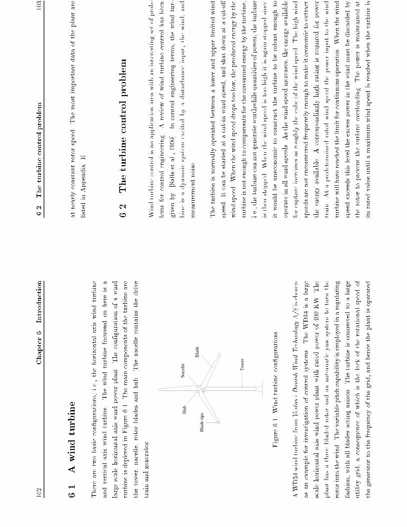
102

Chapter6.Introduction

6.1

A

windturbine

Therearetwobasiccon�gurations,i.e.,thehorizontalaxiswindturbine

andverticalaxiswindturbine.Thewindturbinefocussedonhereisa

largescalehorizontalaxiswindpowerplant.Thecon�gurationofawind

turbineisdepictedinFigure6.1.Themaincomponentsoftheturbineare

thetower,nacelle,rotorbladesandhub.Thenacellecontainsthedrive

trainandgenerator.

Tow

er

Hub

Bla

de ti

ps

Nac

elle

Bla

de

Figure6.1.Windturbinecon�gurations

AWD34windturbinefromVestas-DanishWindTechnologyA/Sischosen

asanexampleforinvestigationofcontrolsystems.TheWD34isalarge

scalehorizontalaxiswindpowerplantwithratedpowerof400KW.The

planthasathreebladedrotorandanautomaticyawsystem

toturnthe

rotorintothewind.Thevariablepitchcapabilityisemployedinaregulating

fashion,withallbladesactingunison.Theturbineisconnectedtoalarge

utilitygrid,aconsequenceofwhichisthelockoftherotationalspeedof

thegeneratortothefrequencyofthegrid,andhencetheplantisoperated

6.2

Theturbinecontrolproblem

103

atnearlyconstantrotorspeed.Themostimportantdataoftheplantare

listedinAppendixE.

6.2

Theturbinecontrolproblem

Windturbinecontrolisanapplicationareawithaninterestingsetofprob-

lemsforcontrolengineering.Areviewofwindturbinecontrolhasbeen

givenby

[Salleetal.,1990].Incontrolengineeringterms,thewindtur-

bineisadynamicsystem

excitedbyadisturbanceinput,thewind,and

measurementnoise.

Theturbineisnormallyoperatedbetweenalowerandupperlimitedwind

speed.Itcanbestartedatacut-inwindspeed,andshutdownatacut-o�

windspeed.Whenthewindspeeddropstoolow,theproducedenergybythe

turbineisnotenoughtocompensatefortheconsumedenergybytheturbine,

i.e.,theturbinecannotgenerateworthwhilequantitiesofpower,theturbine

isthenstopped.Whenthewindspeedistoohighitisagainstoppedsince

itwouldbeuneconomictoconstructtheturbinetoberobustenoughto

operateinallwindspeeds.Asthewindspeedincreases,theenergyavailable

forcaptureincreasesasroughlythecubeofthewindspeed.Thehighwind

speedsarenotencounteredfrequentlyenoughtomakeiteconomictoextract

theenergyavailable.Acorrespondinglyhighratingisrequiredforpower

train.Atapredeterminedratedwindspeedthepowerinputtothewind

turbinewillhavereachedthelimitforcontinuousoperation.Whenthewind

speedexceedsthisleveltheexcesspowerinthewindmustbediscardedby

therotortopreventtheturbineoverloading.Thepowerismaintainedat

itsratedvalueuntilamaximumwindspeedisreachedwhentheturbineis

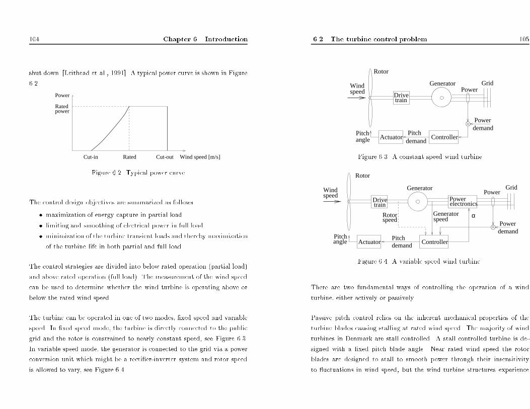
104 Chapter 6. Introduction

shut down [Leithead et al., 1991]. A typical power curve is shown in Figure

6.2.

Rated

Wind speed [m/s]

power

Power

Cut-in Rated Cut-out

Figure 6.2. Typical power curve

The control design objectives are summarized as follows

� maximization of energy capture in partial load.

� limiting and smoothing of electrical power in full load.

� minimization of the turbine transient loads and thereby maximization

of the turbine life in both partial and full load.

The control strategies are divided into below rated operation (partial load)

and above rated operation (full load). The measurement of the wind speed

can be used to determine whether the wind turbine is operating above or

below the rated wind speed.

The turbine can be operated in one of two modes, �xed speed and variable

speed. In �xed speed mode, the turbine is directly connected to the public

grid and the rotor is constrained to nearly constant speed, see Figure 6.3.

In variable speed mode, the generator is connected to the grid via a power

conversion unit which might be a recti�er-inverter system and rotor speed

is allowed to vary, see Figure 6.4.

6.2 The turbine control problem 105

demand

Drive train

Generator

Rotor

Wind speed

Powerdemand

GridPower

ControllerPitchangle Actuator

Pitch

Figure 6.3. A constant speed wind turbine

Power

Rotor

trainDrive

Generator

Generatorspeed

Rotorspeed

Pitchangle

Powerdemand

speedWind

Actuator demandPitch

Controller

α

GridPower

electronics

Figure 6.4. A variable speed wind turbine

There are two fundamental ways of controlling the operation of a wind

turbine, either actively or passively.

Passive pitch control relies on the inherent mechanical properties of the

turbine blades causing stalling at rated wind speed. The majority of wind

turbines in Denmark are stall controlled. A stall controlled turbine is de-

signed with a �xed pitch blade angle. Near rated wind speed the rotor

blades are designed to stall to smooth power through their insensitivity

to uctuations in wind speed, but the wind turbine structures experience

106

Chapter6.Introduction

greatermeanthrustloads[Leitheadetal.,1991].Astallingrotorisself-

regulatingprovidingpowerlimitingandgoodpowerqualitywithoutthe

needforacontrolsystem.Thegoodpowerqualityreferstotheextentof

rapid uctuationsinthegeneratedpowerissmall.Thepassivecontrolwill

notbediscussedinthisreport.

Activecontrolcanbeachievedbycontrollingthebladeangle(pitch),nacelle

rotation(yaw),andturbinerotationalspeed.

Thetorqueinducedontherotorbythewinddependsonthepitchan-

gleoftheblades.Hence,thetorquemaybereducedbyfeatheringand

viceversa.Aboveratedwindspeed,thepitchofthebladesarecontin-

uouslysettotheangleofpitchatwhichratedpowerisgenerated.The

adjustmentofpitchangleisusuallymadeinresponsetopowermeasure-

ment[Leitheadetal.,1992].Pitchcontrolhassofarbeenthedominating

methodforpowercontrol.Improvementinpowerqualityandalleviationof

fatiguedamagecanbeachievedbycontinuouslymonitoringthewindtur-

bineandalteringthepitchangleofthebladesaccordingly.Acontrolsystem

withtheabilitytovarypitchinanactivefeedbackcontrolisrequired.

Thevariablespeedconceptforwindturbinesisstillrelativelyrarelyim-

plemented.Invariablespeedwindturbinesthegeneratordoesnotdirectly

coupletothegrid.Thereforetherotorispermittedtorotateatanyspeed

bythepowergenerationunitwhichmightbeageneratorandafrequency

convertercombination.Forvariablespeedoperationtheremaybemore

thanonecontrolaction.Inthisprojecttheapproachistocombinevariable

speedoperationwithavariablepitchcapabilityinfullload.Thestrategyis

thentoregulatetheloadonthewindturbinebyadjustingtherotorspeed

andpitchangletomaintainpowergenerationatratedvalues.Inpartial

6.3

Outlineofthesecondpartofthethesis

107

loadthepitchangleis�xedatoptimalvalue,acontrollerwithoutpitch

actionthroughthegeneratorreactiontorquewillbeimplemented.The

controlstrategyisthentomaximizeenergycapturebyadjustingtherotor

speedtofollowthewindspeedvariations.

Onbothconstantandvariablespeedturbineselectricalpoweristhemost

readilyavailablemeasurementsignal.Inadditiontoelectricalpowermea-

surement,thegeneratorshaftspeedwillbemeasuredforavariablespeed

turbine.Inthecaseofpartialload,ameasurementofrotorspeedmayalso

berequiredforavariablespeedplant.

6.3

Outlineofthesecondpartofthethesis

Anoutlineofthesecondpartofthethesisisgiveninthissection.

Chapter

6isanintroductiontothewindturbinesystemsandcontrol

problems.Themotivationsbehindthedesigndecisionsareexplained.

Chapter7describesallthesigni�cantdynamicfeaturesencounteredona

practicalwindturbine,withemphasisontheuseofsuchamodelinthe

validationandinvestigationofcontrolsystems.Theresultisageneral

nonlinearmathematicalmodelwhichisusedforsimulations.Themodelis

validatedbyusingthedatafromanexistingWD34windturbine.

Chapter8containssimplelinearmodelsofwindturbineswhichwillbeused

fordesignofcontrollers.Similarmodelsfortheconstantspeedturbineand

108

Chapter6.Introduction

variablespeedturbinearederivedinthischapter.Thedesignmodelsare

madeassimpleaspossiblewhilekeepingallsigni�cantdynamics.

Chapter

9dealswithestimationofthewindspeedinconnectiontoa

windturbine.TheNewton-Raphsonmethod,Kalman�ltermethodand

extendedKalman�ltermethodareinvestigatedforbothpartialloadand

fullload.Theexperimentaldataareusedtotesttheestimationmethods.

Theproblemthatmightbecausedbythemethodsisdiscussedattheend

ofchapter.

Chapter10isconcernedwithcontrolofthewindturbinesinfullload.Both

theconstantspeedandvariablespeedturbineareinvestigated.Theactive

pitchcontrolisthemostpopularcontrolmethodinpracticalapplications.

TheemphasisofthechapterisgiventotheLQG

controlmethodfora

solelypitchcontrolledwindturbine,aswellasacombinedvariablespeed

andpitchcontrolwindturbine.

Chapter11isfocussedoncontrolofavariablespeedwindturbineinpar-

tialload.Belowratedwindspeedthecontrolstrategiesaretomaximizethe

energycapturefromthewindandminimizethetransientloads.Thepitch

angleofrotorbladesis�xedatoptimalvalue,controlwithoutpitchaction

throughthegeneratorreactiontorquewillbeimplemented.TheLQGcon-

trolandtrackingcontrolmethodsareinvestigatedandthetrade-o�hasto

bemadebetweendi�erentcontrolobjectives.Someimplementationconsid-

erationsaregivenattheendofthischapter.

Chapter

12givesasummaryandconclusionsofthesecondpartofthe

thesis.

Chapter7

SimulationModelofthe

WindTurbine

7.1

Introduction

Thischapterprovidesinsightintothemodellingofanentirewindturbine

system.Themotivationistogivetheinformationaboutdynamicsofawind

turbine,withemphasisupontheuseofsuchamodelintheinvestigationof

controlsystems.

Themajorcomponentsofaturbinearethetower,rotor(thebladesand

hub),drivetrainandpowergenerationunit.Thedrivingtrainconsistsof

thelow-speedshaft,gearboxandhigh-speedshaft.Thesimulationmodel

109

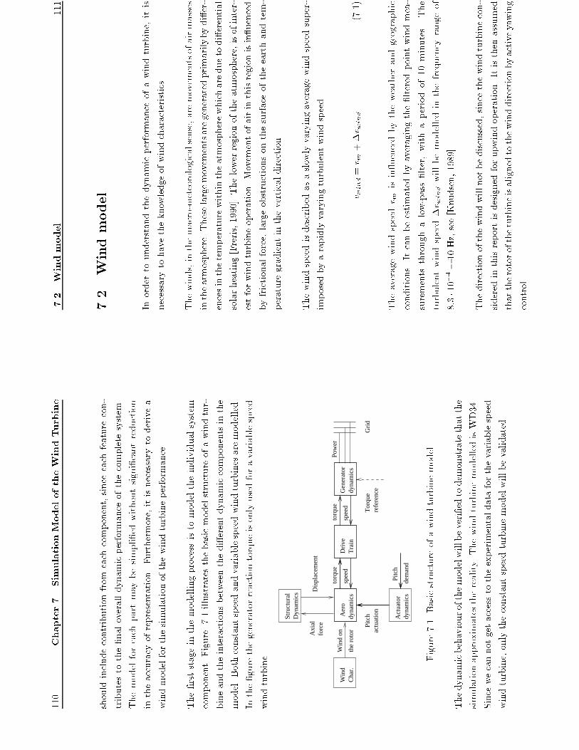
110

Chapter7.SimulationModeloftheWindTurbine

shouldincludecontributionfromeachcomponent,sinceeachfeaturecon-

tributestothe�naloveralldynamicperformanceofthecompletesystem.

Themodelforeachpartmaybesimpli�edwithoutsigni�cantreduction

intheaccuracyofrepresentation.Furthermore,itisnecessarytoderivea

windmodelforthesimulationofthewindturbineperformance.

The�rststageinthemodellingprocessistomodeltheindividualsystem

component.Figure7.1illustratesthebasicmodelstructureofawindtur-

bineandtheinteractionsbetweenthedi�erentdynamiccomponentsinthe

model.Bothconstantspeedandvariablespeedwindturbinesaremodelled.

Inthe�gurethegeneratorreactiontorqueisonlyusedforavariablespeed

windturbine.

the

roto

rA

ero

dyna

mic

sD

rive

Tra

indy

nam

ics

Act

uato

rdy

nam

ics

Gen

erat

orto

rque

spee

d

torq

ue

spee

d

Pitc

h

dem

and

Pitc

hac

tuat

ion

Pow

er

Gri

d

Stru

ctur

alD

ynam

ics D

ispl

acem

ent

Axi

alfo

rce

Cha

r.W

ind

Tor

que

refe

renc

e

Win

d on

Figure7.1.Basicstructureofawindturbinemodel

Thedynamicbehaviourofthemodelwillbeveri�edtodemonstratethatthe

simulationapproximatesthereality.ThewindturbinemodelledisWD34.

Sincewecannotgetaccesstotheexperimentaldataforthevariablespeed

windturbine,onlytheconstantspeedturbinemodelwillbevalidated.

7.2

Windmodel

111

7.2

Windmodel

Inordertounderstandthedynamicperformanceofawindturbine,itis

necessarytohavetheknowledgeofwindcharacteristics.

Thewinds,inthemacro-meteorologicalsense,aremovementsofairmasses

intheatmosphere.Theselargemovementsaregeneratedprimarilybydi�er-

encesinthetemperaturewithintheatmospherewhichareduetodi�erential

solarheating[Freris,1990].Thelowerregionoftheatmosphere,isofinter-

estforwindturbineoperation.Movementofairinthisregionisin uenced

byfrictionalforce,largeobstructionsonthesurfaceoftheearthandtem-

peraturegradientintheverticaldirection.

Thewindspeedisdescribedasaslowlyvaryingaveragewindspeedsuper-

imposedbyarapidlyvaryingturbulentwindspeed.

v wind=v m+�v wind

(7.1)

Theaveragewindspeedv misin uencedbytheweatherandgeographic

conditions.Itcanbeestimatedbyaveragingthe�lteredpointwindmea-

surementsthroughalow-pass�lter,withaperiodof10minutes.The

turbulentwindspeed�v wind

willbemodelledinthefrequencyrangeof

8:3�10�4�10Hz,see[Knudsen,1989].

Thedirectionofthewindwillnotbediscussed,sincethewindturbinecon-

sideredinthisreportisdesignedforupwindoperation.Itisthenassumed

thattherotoroftheturbineisalignedtothewinddirectionbyactiveyawing

control.

112

Chapter7.SimulationModeloftheWindTurbine

Forawindturbine,itisusualtomeasurethewindspeedbyananemometer

situatedonthetopofnacelle.Themeasuredwindspeediscalledpointwind

speed.Althoughthereisnosuchthingasthewindspeedexperiencedby

thewindturbine,sincetherotorissubjecttoaspatiallydistributedwind

�eldwhichvariesintime,theturbinemaybeconsideredtoexperiencean

e�ectivewindspeedwhich,insomesense,isanaverageovertherotordisc.

Thehighfrequenciesofthee�ectivewindspeedexperiencedbytherotor

willbedampedcomparingwiththefrequenciesofthepointwindspeed.

Thissectionwillde�neamodeldescribingthebehaviourofthee�ective

turbulentwindspeedontherotor.Firstofall,apowerspectrum

forthe

pointwindspeedischosenandsimpli�ed.Secondly,by�lteringthepower

spectrumofthepointwindspeedwitha�lterfunction,thepowerspectral

densityfunctionforthee�ectivewindspeedexperiencedbytherotorcan

befound.Finally,alinearmodelwhichhasapproximatelythesamespec-

trumwillbeobtained.Inthisreporttheturbulentwindspeedisassumed

constantoverthewholerotor.

7.2.1

Thepointwindspeed

Themodelofthewindspeedatmeasurementpointis

v wind=v m+v p

(7.2)

wherev pistheturbulentpointwindspeed.

7.2

Windmodel

113

Theturbulentpointwindspeedisdescribedbypowerspectrumgivenby

[H�jstrup,1982]

f�Sp(f)

v2 �0

=

0:5fi

1+2:2f

5 3 i

�(hi�L

)2 3

+

105f ru

(1+33fru)5 3

�(1�h h

i)2

(1+15h h

i)2 3

(7.3)

f iandf ruarede�nedas

f i=

f�hi

v m

(7.4)

f ru=

f�hvm

1+15h h

i

(7.5)

ListofSymbol

v m

themeanwindspeed

[m/s]

v �0

frictionvelocity

[m/s]

h

measuringheight

[m]

hi

heightofconvectiveboundarylayer

[m]hi=1000m

L

Monon-Obukhovlength

[m]

f

frequency

f=

! 2�

[Hz]

Theabovespectrumconsistsoftwoparts.The�rstpartcorrespondstothe

thermalturbulence(lowfrequency)andthesecondpartcorrespondstothe

mechanicalturbulence(highfrequency).

Iftheverticaltemperaturegradientisabout�10oC=km,theairmasswill

neithermoveupnormovedown,thisiscalledneutralcondition.Ifthe

verticaltemperaturegradientislessthan�10oC=km,theairmasswill

moveup,itisanunstableatmosphere;Otherwiseitisastableatmosphere

ifthegradientismorethan�10oC=km.Theunstable,neutralandstable

conditionhappenabout6%,60%and34%oftime[Petersenetal.,1980].

Thereforewechoosetheneutralconditionforthemodel.Foraneutral

114

Chapter7.SimulationModeloftheWindTurbine

conditionthe�rstpartofthemodelcanbeneglected,whichmeansthatthe

highfrequencypartisdominant.Theabovefunctioncanthenbereduced

to

f�Sp(f)

v2 �0

=

105f ru

(1+33f ru)5 3

�(1�h h

i)2

(1+15h h

i)2 3

(7.6)

In[H�jstrup,1982],themodelvarianceisobtainedbyintegrationof(7.6)

overpositivefrequenciesonly

�2 p=

Z 1 0

Sp(f)df=

105

22

(1�h h

i)2

(1+15h h

i)

2 3

v2 �0

(7.7)

Accordingto[Larsenetal.,1992],foraneutralcondition

v �0v m

=

�

ln(h=r l)

(7.8)

where�isvonK�arm�anconstant(�0:4),histhemeasuringheight,r lis

theroughnesslength.Table7.1showsroughnessclassandcorresponding

roughnesslengthfordi�erentlandscapes[Petersenetal.,1980].Areason-

ablechoicefortheroughnesslengthisbetweenclass1and2.

Roughnessclass

Typeoflandscape

Roughnesslengthr l

0

Sea

1mm

1

Opencountry

1cm

2

Farmland

5cm

3

Smalltown

30cm

Table7.1.Roughnessclassandroughnesslengthfordi�erentlandscape

Bychoosingtheroughnesslengthproperly,itisthenpossibletoachieve

thespectraldensityfunctionandthevarianceofthepointwindspeedby

insertingthefrictionvelocityv �0into(7.6)and(7.7).Itcanbeeasilyfound

7.2

Windmodel

115

thatthespectrum

andvarianceofthepointwinddependontheaverage

windspeed.

7.2.2

Thewindexperiencedbytherotor

Itisimpossibletomeasurethewindspeedontherotor,sincethewind

speedvariesoverthediscsweptbytherotor.Thewindexperiencedbythe

rotorcanbeconsideredasanaverageofthespatialturbulence,whichwill

bemodelledbydynamically�lteringthepointwind

Sef(f)=Sp(f)F(f)

(7.9)

Thepowerspectrumofthe�lterisgivenby[Knudsen,1983]

F(f)=

1

(1+

8p�3

R vm

f)(1+4p�R v

m

f)

(7.10)

whereRisrotorradius.

7.2.3

Theapproximatede�ectivewindspeed

Forthepurposeofsimulation,alinearmodelforthee�ectivewindspeed

hastobederived.

Thepowerspectrumofthee�ectivewindspeedSef(f)canbeapproximated

bythepowerspectraldensityfunction

�v(!)=

k2

(1+p2 1!2)(1+p2 2!2)

�e(!)

=H(j!)�e(!)H(�j!)

(7.11)

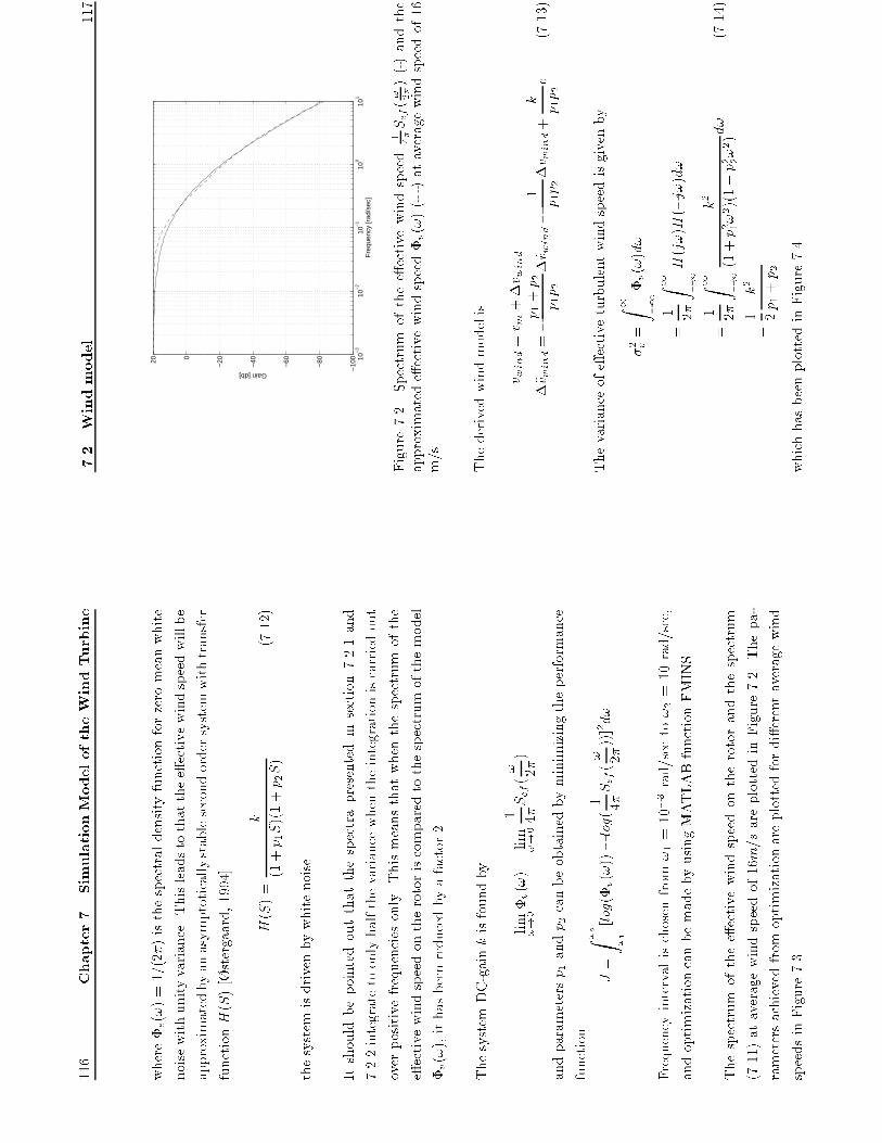
116

Chapter7.SimulationModeloftheWindTurbine

where�e(!)=1=(2�)isthespectraldensityfunctionforzeromeanwhite

noisewithunityvariance.Thisleadstothatthee�ectivewindspeedwillbe

approximatedbyanasymptoticallystablesecondordersystemwithtransfer

functionH(S)[�stergaard,1994]

H(S)=

k

(1+p1S)(1+p2S)

(7.12)

thesystemisdrivenbywhitenoise.

Itshouldbepointedoutthatthespectrapresentedinsection7.2.1and

7.2.2integratetoonlyhalfthevariancewhentheintegrationiscarriedout

overpositivefrequenciesonly.Thismeansthatwhenthespectrumofthe

e�ectivewindspeedontherotoriscomparedtothespectrumofthemodel

�v(!),ithasbeenreducedbyafactor2.

ThesystemDC-gainkisfoundby

lim!!0

�v(!)=lim!!0

1 4�Sef(

! 2�

)

andparametersp1andp2canbeobtainedbyminimizingtheperformance

function

J=

Z !2

!1

[log(�v(!))�log(

1 4�

Sef(

! 2�

))]2d!

Frequencyintervalischosenfrom!1=10�3rad/secto!2=10rad/sec,

andoptimizationcanbemadebyusingMATLABfunctionFMINS.

Thespectrum

ofthee�ectivewindspeedontherotorandthespectrum

(7.11)ataveragewindspeedof16m=sareplottedinFigure7.2.Thepa-

rametersachievedfromoptimizationareplottedfordi�erentaveragewind

speedsinFigure7.3.

7.2

Windmodel

117

10−

310

−2

10−

110

010

1−

100

−80

−60

−40

−20020

Fre

quen

cy [r

ad/s

ec]

Gain [db]

Figure7.2.Spectrum

ofthee�ectivewindspeed

1 4�Sef(! 2�)(-)andthe

approximatede�ectivewindspeed�v(!)(--)ataveragewindspeedof16

m/s

Thederivedwindmodelis

v wind=v m+�v wind

��v wind=�

p1+p2

p1p2

�_v wind�

1p1p2

�v wind+

kp1p2

e

(7.13)

Thevarianceofe�ectiveturbulentwindspeedisgivenby

�2 v=

Z 1 �1

�v(!)d!

=

1 2�

Z 1 �1

H(j!)H(�j!)d!

=

1 2�

Z 1 �1

k2

(1+p2 1!2)(1+p2 2!2)

d!

(7.14)

=1 2

k2

p1+p2

whichhasbeenplottedinFigure7.4.

118

Chapter7.SimulationModeloftheWindTurbine

510

1520

2530

051015 k

510

1520

2530

0204060 p1

510

1520

2530

0

0.51

1.5

Win

d S

peed

[m/s

]

p2

Figure7.3.Parametersk,p1andp2atdi�erentaveragewindspeed

51

01

52

02

53

00123456789

Win

d s

pe

ed

[m

/s]

Variance

Figure7.4.Variancesofthee�ectivewindspeedatdi�erentaveragewind

speeds

7.2

Windmodel

119

Thee�ectivewindspeedsexperiencedbytherotorataveragewindspeeds

of7m/sand16m/sareplottedinFigure7.5.Thewindsequencesare

obtainedfromthesimulations.

02

04

06

08

01

00

12

01

40

16

01

80

20

068

10

12

14

16

18

20

Tim

e [

s]

Wind speed [m/s]

Figure7.5.Simulatedwindattheaveragewindspeedof7m/s(dashed)

and16m/s(solid)

However,thee�ectivewindspeedexperiencedbytherotorhastobemod-

i�edbyincludingthecontributionfromthetowermotion,whichwillbe

explainedinthefollowingsections.

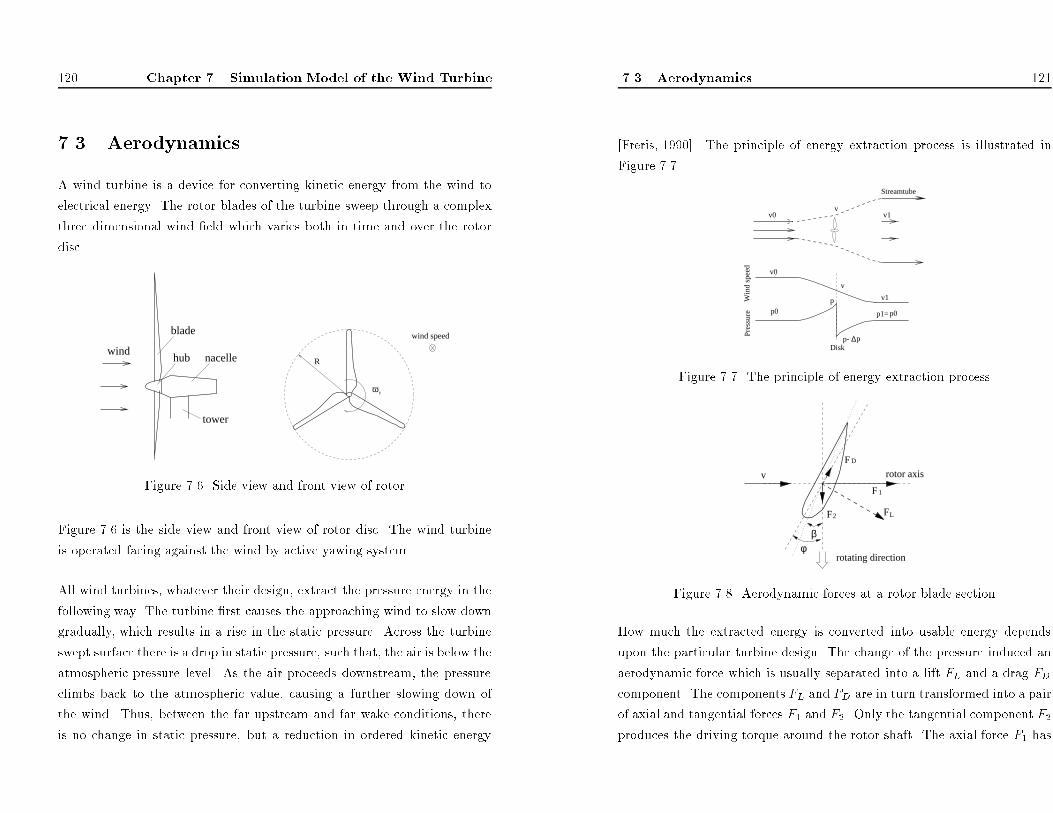
120 Chapter 7. Simulation Model of the Wind Turbine

7.3 Aerodynamics

A wind turbine is a device for converting kinetic energy from the wind to

electrical energy. The rotor blades of the turbine sweep through a complex

three dimensional wind �eld which varies both in time and over the rotor

disc.

tower

wind

blade

hub nacelle R

ω r

wind speed

Figure 7.6. Side view and front view of rotor

Figure 7.6 is the side view and front view of rotor disc. The wind turbine

is operated facing against the wind by active yawing system.

All wind turbines, whatever their design, extract the pressure energy in the

following way. The turbine �rst causes the approaching wind to slow down

gradually, which results in a rise in the static pressure. Across the turbine

swept surface there is a drop in static pressure, such that, the air is below the

atmospheric pressure level. As the air proceeds downstream, the pressure

climbs back to the atmospheric value, causing a further slowing down of

the wind. Thus, between the far upstream and far wake conditions, there

is no change in static pressure, but a reduction in ordered kinetic energy

7.3 Aerodynamics 121

[Freris, 1990]. The principle of energy extraction process is illustrated in

Figure 7.7.

Pre

ssur

e

vv0 v1

Streamtube

v0

v

Disk

p0 p0

p

p- ∆p

v1

p1=

Win

d sp

eed

Figure 7.7. The principle of energy extraction process

L

β

rotating direction

F

F

F

2

1

D

v

φ

rotor axis

F

Figure 7.8. Aerodynamic forces at a rotor blade section

How much the extracted energy is converted into usable energy depends

upon the particular turbine design. The change of the pressure induced an

aerodynamic force which is usually separated into a lift FL and a drag FD

component. The components FL and FD are in turn transformed into a pair

of axial and tangential forces F1 and F2. Only the tangential component F2

produces the driving torque around the rotor shaft. The axial force F1 has

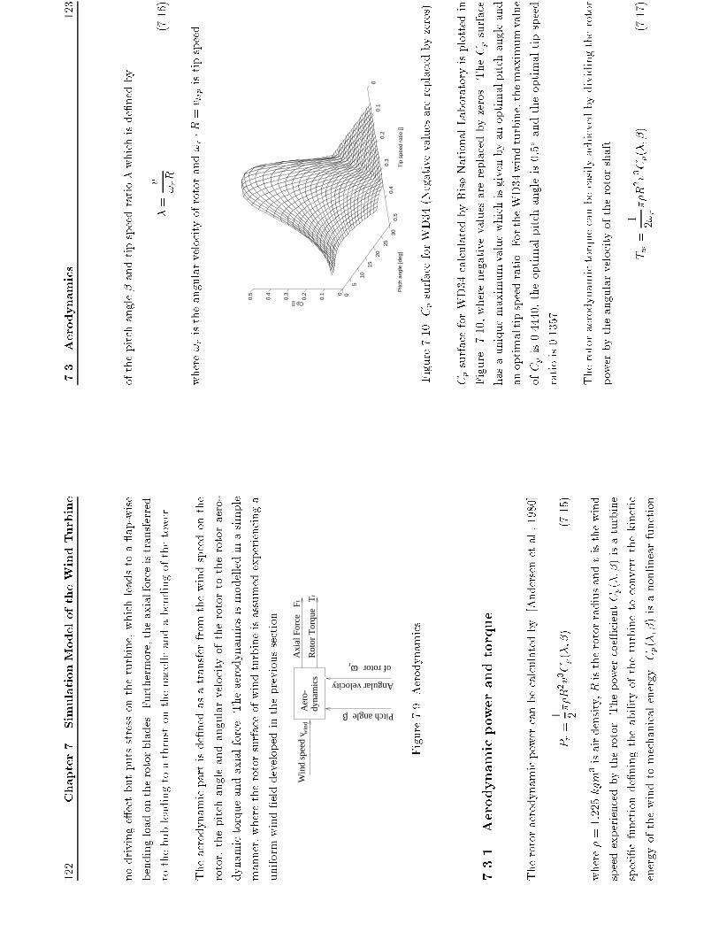
122

Chapter7.SimulationModeloftheWindTurbine

nodrivinge�ectbutputsstressontheturbine,whichleadstoa ap-wise

bendingloadontherotorblades.Furthermore,theaxialforceistransferred

tothehubleadingtoathrustonthenacelleandabendingofthetower.

Theaerodynamicpartisde�nedasatransferfromthewindspeedonthe

rotor,thepitchangleandangularvelocityoftherotortotherotoraero-

dynamictorqueandaxialforce.Theaerodynamicsismodelledinasimple

manner,wheretherotorsurfaceofwindturbineisassumedexperiencinga

uniformwind�elddevelopedintheprevioussection.

Aer

o-dy

nam

ics Angular velocity

of rotor

Pitch angleβ

win

dA

xial

For

ce

Ft

Rot

or T

orqu

eTr

ωr

Win

d sp

eed

v

Figure7.9.Aerodynamics

7.3.1

Aerodynamicpowerandtorque

Therotoraerodynamicpowercanbecalculatedby[Andersenetal.,1980]

Pr=

1 2��R2v3Cp(�;�)

(7.15)

where�=1:225kgm3isairdensity,Ristherotorradiusandvisthewind

speedexperiencedbytherotor.Thepowercoe�cientCp(�;�)isaturbine

speci�cfunctionde�ningtheabilityoftheturbinetoconvertthekinetic

energyofthewindtomechanicalenergy.Cp(�;�)isanonlinearfunction

7.3

Aerodynamics

123

ofthepitchangle�andtipspeedratio�whichisde�nedby

�=

v!rR

(7.16)

where!ristheangularvelocityofrotorand!r�R=v tipistipspeed.

00.

10.

20.

30.

40.

5

0

510

1520

2530

0

0.1

0.2

0.3

0.4

0.5

Pitc

h an

gle

[deg

]T

ip s

peed

rat

io []

Cp []

Figure7.10.CpsurfaceforWD34(Negativevaluesarereplacedbyzeros)

CpsurfaceforWD34calculatedbyRis�NationalLaboratoryisplottedin

Figure7.10,wherenegativevaluesarereplacedbyzeros.TheCpsurface

hasauniquemaximumvaluewhichisgivenbyanoptimalpitchangleand

anoptimaltipspeedratio.FortheWD34windturbine,themaximumvalue

ofCpis0.4440,theoptimalpitchangleis0:5oandtheoptimaltipspeed

ratiois0.1357.

Therotoraerodynamictorquecanbeeasilyachievedbydividingtherotor

powerbytheangularvelocityoftherotorshaft

Tw

=

12!r

��R

2v

3Cp(�;�)

(7.17)

124 Chapter 7. Simulation Model of the Wind Turbine

7.3.2 3p e�ect

As well as the disc averaged torque Tw, the rotor experiences various low

speed torque harmonic associated with the rotational frequency (nP) of the

blades. For a three bladed wind turbine, the most important disturbances

are 3P and 1P peaks with the 3P peak much more pronounced than the 1P

peak.

The spectral peaks are caused by the wind speed turbulence, the wind gra-

dient and shadow of the tower. The wind speed depends on the altitude

above ground, which causes the wind speed to be faster at top of the disc

swept by the rotor than at the lowest part. This is the gradient e�ect.

The tower shadow phenomenon is that when one of the blades sweeps in

front of the supporting tower, the torque induced on the blade will be re-

duced. [Leithead et al., 1992] indicates that the 1P peak is predominantly

deterministic and 3P peak is predominantly stochastic.

The 1P peak modelled by a simple sinusoid with amplitude A is given by

[Wilkie et al., 1990]

TnP = A sin(!rt) (7.18)

The 1P-e�ect is not included in the report.

A suitable model of the 3P peak is given by a lightly damped second order

function with white noise as input [Flensborg and S�rensen, 1995]

T3P (s)

e(s)

=

k3PTw(3!r)2

s2 + 2�(3!r)s+ (3!r)2

(7.19)

The spectrum of the model has a peak at 3!r. The amplitude k3P and

damping ratio � are determined empirically by comparing the model output

with the data sequences obtained from the existing WD34 wind turbine.

7.3 Aerodynamics 125

The total rotor torque experienced by the rotor is then modi�ed by

Tr = Tw + T3P (7.20)

7.3.3 Axial force

The force, induced by the wind on the rotor, causes the bending movement

of the tower in axial direction. The movement is depicted in Figure 7.11.

t

tv Fwind

ω t

h

Figure 7.11. The bending movement of the tower

!t in the �gure is the angular velocity of the bending movement and ht is

the height of the tower. The driving force Ft, assumed acting on the centre

of the rotor, is given by [Andersen et al., 1980]

Ft =1

2��R2v2Ct(�; �) (7.21)

where v is the e�ective wind speed experienced by the rotor, which di�ers

from the wind in front of the rotor due to the tower motion. Therefore v

has to be modi�ed by considering the contribution of the tower movement.

v = vwind � !tht (7.22)

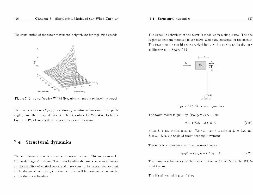
126 Chapter 7. Simulation Model of the Wind Turbine

The contribution of the tower movement is signi�cant for high wind speeds.

00.1

0.20.3

0.40.5

0

510

1520

2530

0

0.5

1

1.5

Pitch angle [deg] Tip speed ratio []

Ct [

]

Figure 7.12. Ct surface for WD34 (Negative values are replaced by zeros)

The force coe�cient Ct(�; �) is a strongly non-linear function of the pitch

angle � and the tip speed ratio �. The Ct surface for WD34 is plotted in

Figure 7.12, where negative values are replaced by zeros.

7.4 Structural dynamics

The axial force on the rotor causes the tower to bend. This may cause the

fatigue damage of turbines. The tower bending dynamics have an in uence

on the stability of control loops and have thus to be taken into account

in the design of controller, i.e., the controller will be designed so as not to

excite the tower bending.

7.4 Structural dynamics 127

The dynamic behaviour of the tower is modelled in a simple way. The one

degree of freedom modelled in the tower is an axial de ection of the nacelle.

The tower can be considered as a rigid body with a spring and a damper,

as illustrated in Figure 7.13

τ

Ftk

D

t

tl

t

mt

ω

Figure 7.13. Structural dynamics

The tower model is given by [Bongers et al., 1990]

mt�lt +Dt_lt + ktlt = Ft (7.23)

where lt is tower displacement. We also have the relation lt = �tht and

_�t = !t. �t is the angle of tower bending movement.

The structure dynamics can then be rewritten as

mtht��t +Dtht _�t + ktht�t = Ft (7.24)

The resonance frequency of the tower motion is 6.9 rad/s for the WD34

wind turbine.

The list of symbol is given below

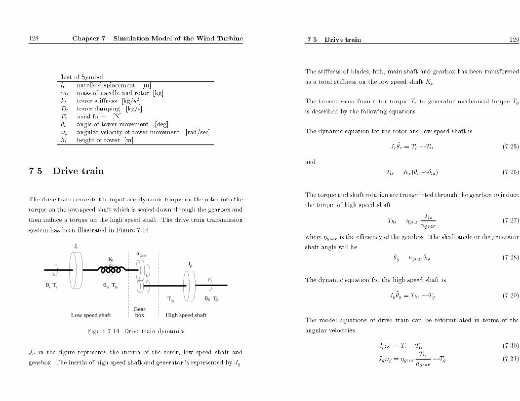
128 Chapter 7. Simulation Model of the Wind Turbine

List of Symbol

lt nacelle displacement [m]

mt mass of nacelle and rotor [kg]

kt tower sti�ness [kg/s2]

Dt tower damping [kg/s]

Ft axial force [N]

�t angle of tower movement [deg]

!t angular velocity of tower movement [rad/sec]

ht height of tower [m]

7.5 Drive train

The drive train converts the input aerodynamic torque on the rotor into the

torque on the low-speed shaft which is scaled down through the gearbox and

then induce a torque on the high speed shaft. The drive train transmission

system has been illustrated in Figure 7.14.

Jr

J

Low speed shaft High speed shaftGearbox

θ Tr r Tls

Ths

Ks

g Tgθ

θls

gearn

g

Figure 7.14. Drive train dynamics

Jr in the �gure represents the inertia of the rotor, low speed shaft and

gearbox. The inertia of high speed shaft and generator is represented by Jg .

7.5 Drive train 129

The sti�ness of blades, hub, main shaft and gearbox has been transformed

as a total sti�ness on the low speed shaft Ks.

The transmission from rotor torque Tr to generator mechanical torque Tg

is described by the following equations.

The dynamic equation for the rotor and low speed shaft is

Jr��r = Tr � Tls (7.25)

and

Tls = Ks(�r � �ls) (7.26)

The torque and shaft rotation are transmitted through the gearbox to induce

the torque of high speed shaftThs = �gear

Tls

ngear

(7.27)

where �gear is the e�ciency of the gearbox. The shaft angle or the generator

shaft angle will be

�g = ngear�ls (7.28)

The dynamic equation for the high speed shaft is

Jg ��g = Ths � Tg (7.29)

The model equations of drive train can be reformulated in terms of the

angular velocities

Jr _!r = Tr � Tls (7.30)

Jg _!g = �gearTls

ngear� Tg (7.31)

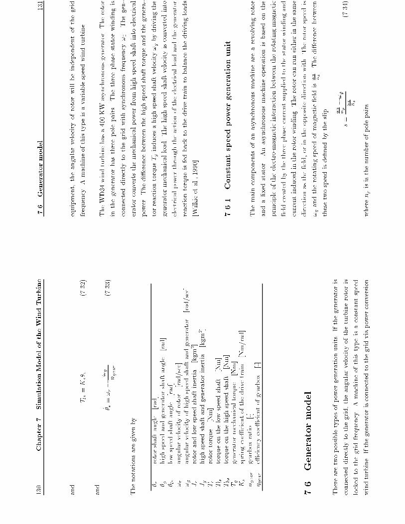
130

Chapter7.SimulationModeloftheWindTurbine

and

Tls=Ks� �

(7.32)

and

_ � �=!r�

!g

ngear

(7.33)

Thenotationsaregivenby

� r

rotorshaftangle

[rad]

� g

highspeedandgeneratorshaftangle

[rad]

� ls

lowspeedshaftangle

[rad]

!r

angularvelocityofrotor

[rad/sec]

!g

angularvelocityofhighspeedshaftandgenerator

[rad/sec]

Jr

rotorandlowspeedshaftinertia

[kgm2]

Jg

highspeedshaftandgeneratorinertia

[kgm2]

Tr

rotortorque

[Nm]

Tls

torqueonthelowspeedshaft

[Nm]

Ths

torqueonthehighspeedshaft

[Nm]

Tg

generatormechanicaltorque

[Nm]

Ks

springcoe�cientofthedrivetrain

[Nm/rad]

ngear

gearboxratio

[-]

�gear

e�ciencycoe�cientofgearbox

[-]

7.6

Generatormodel

Therearetwopossibletypesofpowergenerationunits.Ifthegeneratoris

connecteddirectlytothegrid,theangularvelocityoftheturbinerotoris

lockedtothegridfrequency.Amachineofthistypeisaconstantspeed

windturbine.Ifthegeneratorisconnectedtothegridviapowerconversion

7.6

Generatormodel

131

equipment,theangularvelocityofrotorwillbeindependentofthegrid

frequency.Amachineofthistypeisavariablespeedwindturbine.

TheWD34windturbinehasa400KW

asynchronousgenerator.Therotor

inthegeneratorhasthreepolepairs.Thethreephasestatorwindingis

connecteddirectlytothegridwithsynchronousfrequency!0.Thegen-

eratorconvertsthemechanicalpowerfromhighspeedshaftintoelectrical

power.Thedi�erencebetweenthehighspeedshafttorqueandthegenera-

torreactiontorqueTginducesahighspeedshaftvelocity!gbydrivingthe

generatormechanicalload.Thehighspeedshaftvelocityisconvertedinto

electricalpowerthroughtheactionoftheelectricalloadandthegenerator

reactiontorqueisfedbacktothedrivetraintobalancethedrivingloads

[Wilkieetal.,1990].

7.6.1

Constantspeedpowergenerationunit

Themaincomponentsofanasynchronousmachinearearevolvingrotor

anda�xedstator.Anasynchronousmachineoperationisbasedonthe

principleoftheelectro-magneticinteractionbetweentherotatingmagnetic

�eldcreatedbythethreephasecurrentsuppliedtothestatorwindingand

currentinducedintherotorwinding.Therotorcanruneitherinthesame

directionasthe�eld,orintheoppositedirectionwith.Therotorspeedis

!gandtherotatingspeedofmagnetic�eldis!0

np.Thedi�erencebetween

thesetwospeedisde�nedbytheslip

s=

!0

np

�!g

!0

np

(7.34)

wherenpisisthenumberofpolepairs.

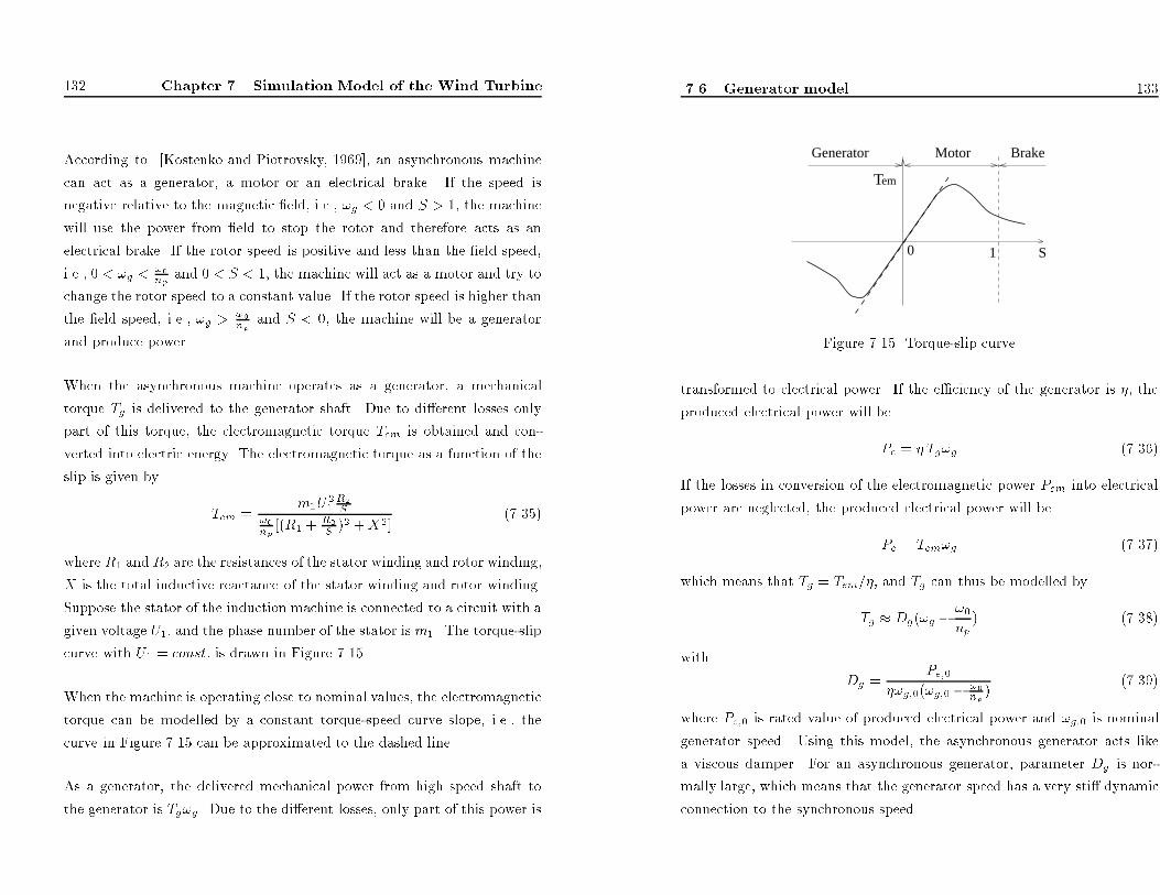
132 Chapter 7. Simulation Model of the Wind Turbine

According to [Kostenko and Piotrovsky, 1969], an asynchronous machine

can act as a generator, a motor or an electrical brake. If the speed is

negative relative to the magnetic �eld, i.e., !g < 0 and S > 1, the machine

will use the power from �eld to stop the rotor and therefore acts as an

electrical brake. If the rotor speed is positive and less than the �eld speed,

i.e., 0 < !g <!0npand 0 < S < 1, the machine will act as a motor and try to

change the rotor speed to a constant value. If the rotor speed is higher than

the �eld speed, i.e., !g >

!0np

and S < 0, the machine will be a generator

and produce power.

When the asynchronous machine operates as a generator, a mechanical

torque Tg is delivered to the generator shaft. Due to di�erent losses only

part of this torque, the electromagnetic torque Tem is obtained and con-

verted into electric energy. The electromagnetic torque as a function of the

slip is given by

Tem =

m1U21

R2S

!0np[(R1 +R2S

)2 +X2]

(7.35)

where R1 and R2 are the resistances of the stator winding and rotor winding,

X is the total inductive reactance of the stator winding and rotor winding.

Suppose the stator of the induction machine is connected to a circuit with a

given voltage U1, and the phase number of the stator is m1. The torque-slip

curve with U1 = const: is drawn in Figure 7.15.

When the machine is operating close to nominal values, the electromagnetic

torque can be modelled by a constant torque-speed curve slope, i.e., the

curve in Figure 7.15 can be approximated to the dashed line.

As a generator, the delivered mechanical power from high speed shaft to

the generator is Tg!g. Due to the di�erent losses, only part of this power is

7.6 Generator model 133

em

0 1 S

Motor BrakeGenerator

T

Figure 7.15. Torque-slip curve

transformed to electrical power. If the e�ciency of the generator is �, the

produced electrical power will bePe = � Tg!g (7.36)

If the losses in conversion of the electromagnetic power Pem into electrical

power are neglected, the produced electrical power will be

Pe = Tem!g (7.37)

which means that Tg = Tem=�, and Tg can thus be modelled by

Tg � Dg(!g � !0np

) (7.38)

with

Dg =

Pe;0

�!g;0(!g;0 � !0np)

(7.39)

where Pe;0 is rated value of produced electrical power and !g;0 is nominal

generator speed. Using this model, the asynchronous generator acts like

a viscous damper. For an asynchronous generator, parameter Dg is nor-

mally large, which means that the generator speed has a very sti� dynamic

connection to the synchronous speed.

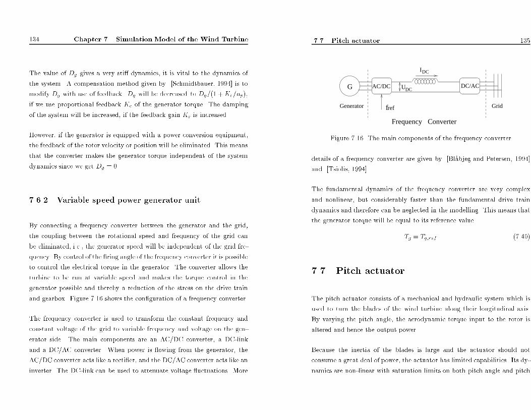
134 Chapter 7. Simulation Model of the Wind Turbine

The value of Dg gives a very sti� dynamics, it is vital to the dynamics of

the system. A compensation method given by [Schmidtbauer, 1994] is to

modify Dg with use of feedback. Dg will be decreased to Dg=(1 +Kc=np),

if we use proportional feedback Kc of the generator torque. The damping

of the system will be increased, if the feedback gain Kc is increased.

However, if the generator is equipped with a power conversion equipment,

the feedback of the rotor velocity or position will be eliminated. This means

that the converter makes the generator torque independent of the system

dynamics since we get Dg = 0.

7.6.2 Variable speed power generator unit

By connecting a frequency converter between the generator and the grid,

the coupling between the rotational speed and frequency of the grid can

be eliminated, i.e., the generator speed will be independent of the grid fre-

quency. By control of the �ring angle of the frequency converter it is possible

to control the electrical torque in the generator. The converter allows the

turbine to be run at variable speed and makes the torque control in the

generator possible and thereby a reduction of the stress on the drive train

and gearbox. Figure 7.16 shows the con�guration of a frequency converter.

The frequency converter is used to transform the constant frequency and

constant voltage of the grid to variable frequency and voltage on the gen-

erator side. The main components are an AC/DC converter, a DC-link

and a DC/AC converter. When power is owing from the generator, the

AC/DC converter acts like a recti�er, and the DC/AC converter acts like an

inverter. The DC-link can be used to attenuate voltage uctuations. More

7.7 Pitch actuator 135

Grid

DC

fref

G AC/DC DC/AC

Generator

ConverterFrequency

UDC

I

Figure 7.16. The main components of the frequency converter

details of a frequency converter are given by [Bl�abjeg and Petersen, 1994]

and [Tsiolis, 1994].

The fundamental dynamics of the frequency converter are very complex

and nonlinear, but considerably faster than the fundamental drive train

dynamics and therefore can be neglected in the modelling. This means that

the generator torque will be equal to its reference value

Tg = Tg;ref (7.40)

7.7 Pitch actuator

The pitch actuator consists of a mechanical and hydraulic system which is

used to turn the blades of the wind turbine along their longitudinal axis.

By varying the pitch angle, the aerodynamic torque input to the rotor is

altered and hence the output power.

Because the inertia of the blades is large and the actuator should not

consume a great deal of power, the actuator has limited capabilities. Its dy-

namics are non-linear with saturation limits on both pitch angle and pitch

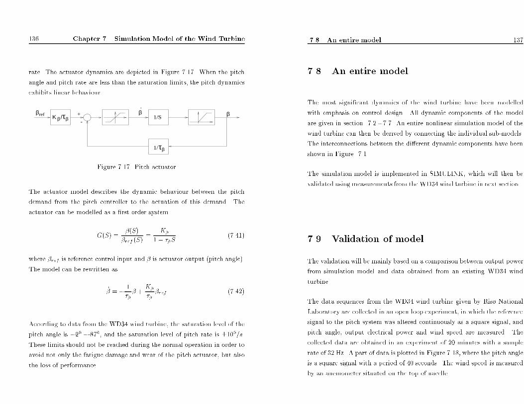
136 Chapter 7. Simulation Model of the Wind Turbine

rate. The actuator dynamics are depicted in Figure 7.17. When the pitch

angle and pitch rate are less than the saturation limits, the pitch dynamics

exhibits linear behaviour.

.

Κβ τβ/ +-

βref1/S

1/τβ

ββ

Figure 7.17. Pitch actuator

The actuator model describes the dynamic behaviour between the pitch

demand from the pitch controller to the actuation of this demand. The

actuator can be modelled as a �rst order system

G(S) =

�(S)

�ref (S)=

K�

1 + ��S

(7.41)

where �ref is reference control input and � is actuator output (pitch angle).

The model can be rewritten as_� = � 1��

� +K�

���ref (7.42)

According to data from the WD34 wind turbine, the saturation level of the

pitch angle is �20 � 870, and the saturation level of pitch rate is �100=s.

These limits should not be reached during the normal operation in order to

avoid not only the fatigue damage and wear of the pitch actuator, but also

the loss of performance.

7.8 An entire model 137

7.8 An entire model

The most signi�cant dynamics of the wind turbine have been modelled

with emphasis on control design. All dynamic components of the model

are given in section 7.2 - 7.7. An entire nonlinear simulation model of the

wind turbine can then be derived by connecting the individual sub-models.

The interconnections between the di�erent dynamic components have been

shown in Figure 7.1.

The simulation model is implemented in SIMULINK, which will then be

validated using measurements from the WD34 wind turbine in next section.

7.9 Validation of model

The validation will be mainly based on a comparison between output power

from simulation model and data obtained from an existing WD34 wind

turbine.

The data sequences from the WD34 wind turbine given by Ris� National

Laboratory are collected in an open loop experiment, in which the reference

signal to the pitch system was altered continuously as a square signal, and

pitch angle, output electrical power and wind speed are measured. The

collected data are obtained in an experiment of 20 minutes with a sample

rate of 32 Hz. A part of data is plotted in Figure 7.18, where the pitch angle

is a square signal with a period of 40 seconds. The wind speed is measured

by an anemometer situated on the top of nacelle.

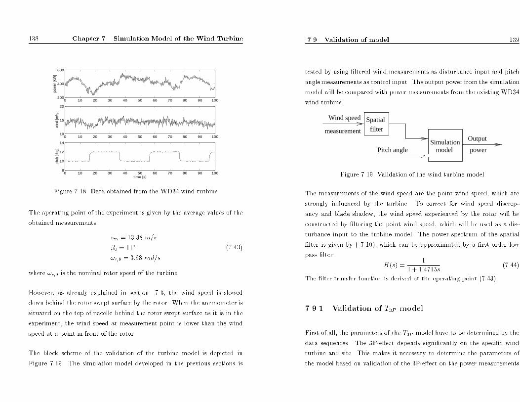
138 Chapter 7. Simulation Model of the Wind Turbine

0 10 20 30 40 50 60 70 80 90 100200

400

600

pow

er [K

W]

0 10 20 30 40 50 60 70 80 90 10010

15

20

win

d [m

/s]

0 10 20 30 40 50 60 70 80 90 1008

10

12

14

time [s]

pitc

h [d

eg]

Figure 7.18. Data obtained from the WD34 wind turbine

The operating point of the experiment is given by the average values of the

obtained measurements

vm = 13:38 m=s

�0 = 11o

!r;0 = 3:68 rad=s

(7.43)

where !r;0 is the nominal rotor speed of the turbine.

However, as already explained in section 7.3, the wind speed is slowed

down behind the rotor swept surface by the rotor. When the anemometer is

situated on the top of nacelle behind the rotor swept surface as it is in the

experiment, the wind speed at measurement point is lower than the wind

speed at a point in front of the rotor.

The block scheme of the validation of the turbine model is depicted in

Figure 7.19. The simulation model developed in the previous sections is

7.9 Validation of model 139

tested by using �ltered wind measurements as disturbance input and pitch

angle measurements as control input. The output power from the simulation

model will be compared with power measurements from the existing WD34

wind turbine.

measurement

Wind speed

powerPitch angle

Spatialfilter

Simulationmodel

Output

Figure 7.19. Validation of the wind turbine model

The measurements of the wind speed are the point wind speed, which are

strongly in uenced by the turbine. To correct for wind speed discrep-

ancy and blade shadow, the wind speed experienced by the rotor will be

constructed by �ltering the point wind speed, which will be used as a dis-

turbance input to the turbine model. The power spectrum of the spatial

�lter is given by ( 7.10), which can be approximated by a �rst order low

pass �lter

H(s) =

1

1 + 1:4715s

(7.44)

The �lter transfer function is derived at the operating point (7.43).

7.9.1 Validation of T3P model

First of all, the parameters of the T3P model have to be determined by the

data sequences. The 3P-e�ect depends signi�cantly on the speci�c wind

turbine and site. This makes it necessary to determine the parameters of

the model based on validation of the 3P-e�ect on the power measurements

140

Chapter7.SimulationModeloftheWindTurbine

fromtheturbine.ItcanbeshownbythepowermeasurementsinFigure

7.20thatthe3Pvariationsintheoutputpowerareabout10%ofthepower

output.

20

30

40

50

60

70

80

90

25

0

30

0

35

0

40

0

45

0

50

0

55

0

60

0

tim

e [s]

power [KW]

Figure7.20.PowermeasurementsoftheWD34windturbine

Theamplitudek3P

anddampingratio�inthemodel(7.19)willbedeter-

minedinsuchawaythattheamplitudeofvariationscausedby3Pe�ectwill

reach10%oftheoutputpower.Thek3P

and�aremutuallydependent.The

powerspectrumofthesimulationoutputandpowermeasurementsobtained

fromtheWD34turbinearegiveninFigure7.21.Thegoodagreementof

theresonancepeakfrequencieshasbeenshowninthe�gure.Theresonance

peakof3P-e�ectisat11rad/swhichisequalto3!r;0.

7.9.2

Validationresults

Theoutputelectricalpowersfromthesimulationmodelandtheexisting

WD34windturbineareshowninFigure7.22.Theaveragevalueofthe

powermeasurementsfromWD34is� PWD34=358:61KW.However,theav-

eragevalueofthesimulationoutputis� Pmodel=261:39KW.Thedi�erence

7.9

Validationofmodel

141

10

−1

10

01

01

10

21

0−

3

10

−2

10

−1

10

0

10

1

10

2

10

3

10

4

10

5

fre

qu

en

cy (

ra

d/s

ec)

SP

EC

TR

UM

ou

tpu

t #

1

Figure7.21.Powerspectrum

forpowermeasurementsfromWD34wind

turbine(solid)andsimulationmodel(dashed).

is�P=

� PWD34�� Pmodel=97:22KW.InFigure7.22theoutputpower

fromsimulationmodelissuperimposedbythedi�erence�P.

50

10

01

50

20

02

50

30

01

50

20

0

25

0

30

0

35

0

40

0

45

0

50

0

55

0

tim

e [

s]

power [KW]

Figure7.22.Outputpowerfromsimulationmodel(solid)andpowermea-

surementsfromtheWD34windturbine(dashed)

Thedi�erence�Piscausedbythelowerwindspeedusedasthedisturbance

inputtothesimulationmodel.Themeasurementsofthewindspeedislower

thanthewindspeedatapointjustinfrontofrotorbecauseofthein uence

oftheturbine.

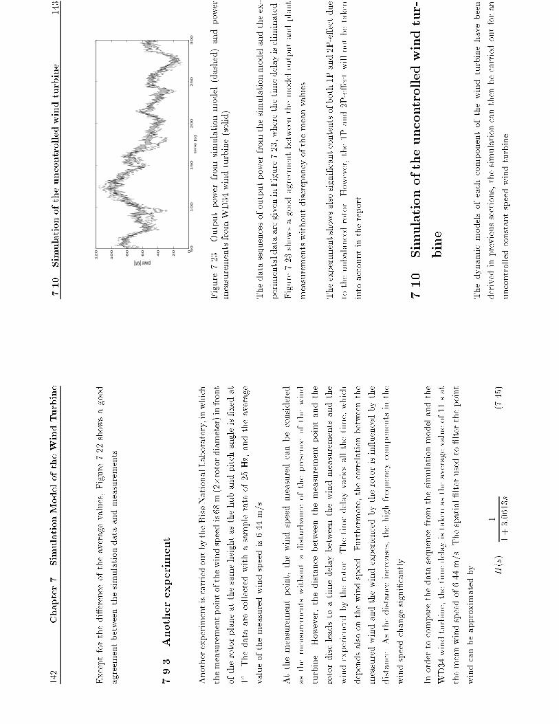
142

Chapter7.SimulationModeloftheWindTurbine

Exceptforthedi�erenceoftheaveragevalues,Figure7.22showsagood

agreementbetweenthesimulationdataandmeasurements.

7.9.3

Anotherexperiment

AnotherexperimentiscarriedoutbytheRis�NationalLaboratory,inwhich

themeasurementpointofthewindspeedis68m(2�rotordiameter)infront

oftherotorplaneatthesameheightasthehubandpitchangleis�xedat

1o.Thedataarecollectedwithasamplerateof25Hz,andtheaverage

valueofthemeasuredwindspeedis6.44m/s.

Atthemeasurementpoint,thewindspeedmeasuredcanbeconsidered

asthemeasurementswithoutadisturbanceofthepresenceofthewind

turbine.However,thedistancebetweenthemeasurementpointandthe

rotordiscleadstoatimedelaybetweenthewindmeasurementsandthe

windexperiencedbytherotor.Thetimedelayvariesallthetime,which

dependsalsoonthewindspeed.Furthermore,thecorrelationbetweenthe

measuredwindandthewindexperiencedbytherotorisin uencedbythe

distance.Asthedistanceincreases,thehighfrequencycomponentsinthe

windspeedchangesigni�cantly.

Inordertocomparethedatasequencefromthesimulationmodelandthe

WD34windturbine,thetimedelayistakenastheaveragevalueof11sat

themeanwindspeedof6.44m/s.Thespatial�lterusedto�lterthepoint

windcanbeapproximatedby

H(s)=

1

1+3:0613s

(7.45)

7.10

Simulationoftheuncontrolledwindturbine

143

50

10

01

50

20

02

50

30

00

20

40

60

80

10

0

12

0

tim

e [

s]

power [KW]

Figure7.23.Outputpowerfrom

simulationmodel(dashed)andpower

measurementsfromWD34windturbine(solid)

Thedatasequencesofoutputpowerfromthesimulationmodelandtheex-

perimentaldataaregiveninFigure7.23,wherethetimedelayiseliminated.

Figure7.23showsagoodagreementbetweenthemodeloutputandplant

measurementswithoutdiscrepancyofthemeanvalues.

Theexperimentshowsalsosigni�cantcontentsofboth1Pand2P-e�ectdue

totheunbalancedrotor.However,the1Pand2P-e�ectwillnotbetaken

intoaccountinthereport.

7.10

Simulationoftheuncontrolledwindtur-

bine

Thedynamicmodelsofeachcomponentofthewindturbinehavebeen

derivedinprevioussections,thesimulationcanthenbecarriedoutforan

uncontrolledconstantspeedwindturbine.

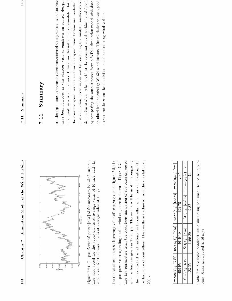
144

Chapter7.SimulationModeloftheWindTurbine

50

60

70

80

90

10

01

10

12

01

30

14

01

50

10

0

20

0

30

0

40

0

50

0

60

0

70

0

Tim

e [

s]

Power [KW]

Figure7.24.Outputelectricalpower[KW]oftheuncontrolledwindturbine.

Thewindspeedfortheupperplotisataveragevalueof16m/s,andthe

windspeedforthelowerplotisataveragevalueof7m/s.

Forthewindsequencewithaveragevalueof16m/sgiveninFigure7.5,the

outputpowercorrespondingtothiswindsequenceisshowninFigure7.24.

Thekeyparametersfromtheopen-loopsimulationoftheconstantspeed

windturbinearegiveninTable7.2.Theresultswillbeusedforcomparing

theuncontrolledwindturbinewithcontrolledwindturbinetoshowthe

performanceofcontrollers.Theresultsareachievedfromthesimulationof

200s.

mean(Pe)[KW]

mean(Tg)[Nm]

mean(!g)[rad/s]

max(ht!t)[cm]

408.05

4010.19

105.79

2.35

SD(Pe)[KW]

SD(Tg)[Nm]

SD(!g)[rad/s]

max(ht�t)[cm]

123.25

1199.20

0.32

3.72

Table7.2.Statisticsobtainedwhilesimulatingtheuncontrolledwindtur-

bine.Meanwindspeedis16m/s.

7.11

Summary

145

7.11

Summary

Allthesigni�cantdynamicfeaturesencounteredonapracticalwindturbine

havebeenincludedinthischapterwithanemphasisoncontroldesign.

Theresultisanonlinearmodelbasedontheindividualsub-models.Both

theconstantspeedturbineandvariablespeedwindturbinearemodelled.

Thesimulationmodelisderivedbycombiningtheanalyticmethodsand

simulationstudies.Themodeloftheconstantspeedturbineisvalidated

bycomparingtheoutputpowerfromaWD34simulationmodelwithdata

obtainedfromanexistingWD34windturbine.Thevalidationshowsagood

agreementbetweenthesimulationmodelandexistingwindturbine.

146

Chapter7.SimulationModeloftheWindTurbine

Chapter8

DesignModeloftheWind

Turbine

Anappropriatemodelofsystem

behaviouristheheartofcontroldesign.

Althoughanonlinearmodelisrequiredforthesimulation,asimplelinear

modelispreferredforcontroldesignpurpose.

Ane�ectivecontrolalgorithmmustre ecttheplantdynamiccharacteristics

aswellastheanticipatedworkingenvironment.Hence,thecontrolproblem

isconvenientlydividedintotwotimescalescorrespondingtoslowmean

windspeedchangesandrapidturbulentwindspeedvariations.Themean

speedsaretreatedassteadystateoperatingpoints.

147

148

Chapter8.DesignModeloftheWindTurbine

Thedesignmodelisthereforesplitintotwoparts:onepartdescribesthe

operatingpointandanotherpartdescribesthedynamicsofthesystembya

linearstate-spacemodel.Theoperatingpointdeterminestheoutputwhen

thesystemisatanequilibrium.Thelinearstate-spacemodeldescribesthe

deviationfromtheoperatingpointwhenthesystemisexcited.Thecontrol

modelcorrespondstoalinearizationabouttheoperatingpoint.

Tofacilitatecontrolsystemdesign,themodelsarerequiredtobeassimpleas

possiblewhileretainingallsigni�cantdynamiccomponentswhichinclude

theaerodynamics,theactuatordynamics,thedrivetrainandgenerator

dynamics.Thewindmodeland3P-e�ectwillalsobeincludedasnoise

models.Thestructuraldynamicsisnotincludedindesignmodels,since

ithasbeenshownbysimulationthatnosigni�cantimprovementcanbe

achievedbyincludingthetowermodel.However,bynotingpositionof

resonance,thetowermotionwillbesuppressedifitisnecessary.

Thischapterisorganizedasfollows.Section8.1givesalinearstate-space

modeloftheturbine,inwhichlinearmodelsofaerodynamictorque,drive

trainandgeneratordynamicswillbederived�rst.Thenthemodelsare

representedforbelowratedoperationandaboveratedoperationseparately.

Section

8.2describesthenoisemodelswhichincludethewindmodeland

T3P

model.Acompositemodelisgiveninsection8.3.Thesampleratesof

digitalcontrollerswillbediscussedinsection8.4,anddiscrete-timemodel

willbeformulated.Asummaryisgivenin8.5.

8.1

Linearstate-spacemodelsoftheplant

149

8.1

Linearstate-spacemodelsoftheplant

8.1.1

Aerodynamictorque

TheaerodynamictorqueTrgivenby(7.17)and(7.20)insection7.3.1is

anonlinearfunctionofthewindspeed,pitchangleandangularvelocityof

rotor

Tr=f(v;�;!r)

(8.1)

Thenonlinearaerodynamictorquecanbelinearizedaroundanoperating

point

Tr=Tw;0+�Tw+�T3P

(8.2)

where

�Tw

=

@Tw@v

� � � � op�v+

@Tw@�

� � � � op��+

@Tw

@!r

� � � � op�!r

(8.3)

and

�v=v�v m

��=���0

(8.4)

�!r=!r�!r;0

wherev m,�0

!r;0

andTw;0

de�neasteady-stateoperatingpoint.�v,

��,�!r,�Tw

and�T3P

areonlysmallchangesfrom

thesteady-state

operatingpoint.@Tw=@v,@Tw=@�and@Tw=@!rarethepartialderivatives

ofaerodynamictorquewithrespecttothewindspeed,pitchangleand

rotorspeedattheoperatingpointaboutwhichthesystem

islinearized.

ThederivativescanbecalculatedfromCpcurveaccordingtotheoperating

150

Chapter8.DesignModeloftheWindTurbine

point

@Tw@v

=

32!r

��R

2v

2Cp+

12!2 r��Rv

3@Cp

@�

@Tw@�

=

12!r

��R2v3@Cp

@�

(8.5)

@Tw

@!r

=�

12!2 r��R2v3Cp�

12!3 r��Rv4@Cp

@�

@Cp=@�and@Cp=@�canbenumericallycalculatedfromCpsurface.

8.1.2

Drivetrainandgenerator

Thedrivetraindynamicscanberepresentedby

�_ � �=�!r�

1ngear

�!g

�_!r=�

KsJr

�� �+

1 Jr

�Tr

(8.6)

�_!g=

�gearKs

ngearJg

�� ��

1 Jg

�Tg

Foraconstantspeedwindturbine,thegeneratorreactiontorqueismodelled

by�Tg=Dg�!g,anditisequaltogeneratortorquereferenceforavariable

speedwindturbine,i.e.,�Tg=�Tg;ref.

8.1.3

Abovetheratedwindspeed

AsalreadystatedinChapter6,whenthewindspeedexceedstherated

value,theobjectivesofthecontrolaretomaintainthepoweratitsrated

8.1

Linearstate-spacemodelsoftheplant

151

valueandpreventturbineoverloading.Bothconstantspeedandvariable

speedturbineareinvestigatedforthispurpose.

Sincethestructuraldynamicsisnotincludedindesignmodels,thewind

speedexperiencedbytherotorcanthenbeapproximatedby�v=�v wind.

Ifpitchsystem

dynamicsisincludedinthemodelandpitchreferenceis

takenasacontrolinput,astate-spacemodeloftheconstantspeedwind

turbinewillberepresented

2 6 6 6 6 4�_ � �

�_!r

�_!g

�_ �

3 7 7 7 7 5=2 6 6 6 6 40

1

�1ngear

0

�Ks

Jr

1 Jr

@Tw

@!r

0

1 Jr

@Tw

@�

�gearKs

ngearJg

0

�DgJg

0

0

0

0

�1 �

�

3 7 7 7 7 52 6 6 6 6 4�� �

�!r

�!g

��

3 7 7 7 7 5

+2 6 6 6 6 40 0 0 K

���

3 7 7 7 7 5��ref+

2 6 6 6 6 40

1 Jr

@Tw

@v

0 0

3 7 7 7 7 5�v wind+

2 6 6 6 6 40 1 Jr 0 0

3 7 7 7 7 5�T3P

(8.7)

Foraconstantspeedwindturbine,theoutputelectricalpowercanbeap-

proximatedbyPe=�Tg(1�S)!0

np,whereSistheslipde�nedby(7.34)at

operatingpoint,theoutputequationofthestate-spacemodelwillthenbe

�Pe=[00

�(1�S)!0

np

Dg

0]2 6 6 6 6 4�

� �

�!r

�!g

��

3 7 7 7 7 5

(8.8)

Avariablespeedwindturbinehastwoinputs,i.e.,thepitchreferenceand

generatortorquereference.Astate-spacemodelforavariablespeedturbine

152

Chapter8.DesignModeloftheWindTurbine

isde�nedby

2 6 6 6 6 4�_ � �

�_!r

�_!g

�_ �

3 7 7 7 7 5=2 6 6 6 6 40

1

�1ngear

0

�Ks

Jr

1 Jr

@Tw

@!r

0

1 Jr

@Tw

@�

�gearKs

ngearJg

0

0

0

0

0

0

�1 �

�

3 7 7 7 7 52 6 6 6 6 4�� �

�!r

�!g

��

3 7 7 7 7 5

+2 6 6 6 6 40

0

0

0

0

�1 J

g

K���

0

3 7 7 7 7 5" ��ref

�Tg;ref

# +2 6 6 6 6 40

1 Jr

@Tw

@v

0 0

3 7 7 7 7 5�v wind+

2 6 6 6 6 40 1 Jr 0 0

3 7 7 7 7 5�T3P

(8.9)

Forawindturbine,inadditiontopowermeasurement,ameasurementof

generatorshaftspeedmayalsobemade.Thegeneratortorquecaneasily

bederivedfromthesetwomeasurements.Theangularvelocityofgenerator

shaft!gandthegeneratorreactiontorquewillthenbechosenasoutputs

foravariablespeedwindturbine[LeitheadandConnor,1994].

" �!g

�Tg

# =" 0

0

1

0

0

0

0

0#2 6 6 6 6 4�� �

�!r

�!g

��

3 7 7 7 7 5+" 0

0

0

1#"��ref

�Tg;ref

#(8.10)

Ageneralizedrepresentationofthestate-spacemodeloftheplantisgiven

by

_xp

=

Apxp+Bpu+Lp1�v wind+Lp2�T3P

y

=

Cpxp+Dpu

(8.11)

wherexp

=[�� �;�!r;�!g;��]T,u=��ref,y=�PeandDP

=0fora

constantspeedplant,andu=[��ref;�Tg;ref]T,y=[�!g;�Tg]Tfora

variablespeedplant.

8.1

Linearstate-spacemodelsoftheplant

153

AbodediagramforaconstantspeedmodelisgiveninFigure8.1,where

theoperatingpointoftheturbineis

v m=16m=s

�0=12:34o

!r;0=3:68rad=s

Pe;0=400KW

(8.12)

10−

110

010

110

210

3−

100

−5005010

0

Fre

quen

cy (

rad/

sec)

Gain dB

10−

110

010

110

210

3

−18

00

180

Fre

quen

cy (

rad/

sec)

Phase deg

Figure8.1.Bodeplotforaconstantspeedwindturbinemodel:fromrefer-

encepitchangle��reftooutputelectricalpower�Pe.

Atthisoperatingpoint,theeigenvaluesoftheconstantspeedturbinemodel

aregiveninTable8.1.Theeigenvaluesofthedrivetraincausetheresonance

peakof6.13rad/sinthebodeplot.

Eigenvalue

subsystem

-1.3167�5.9913i

drivetrain

-169.2580

generator

-2.8571

actuator

Table8.1.Eigenvaluesforthemodelofaconstantspeedturbine

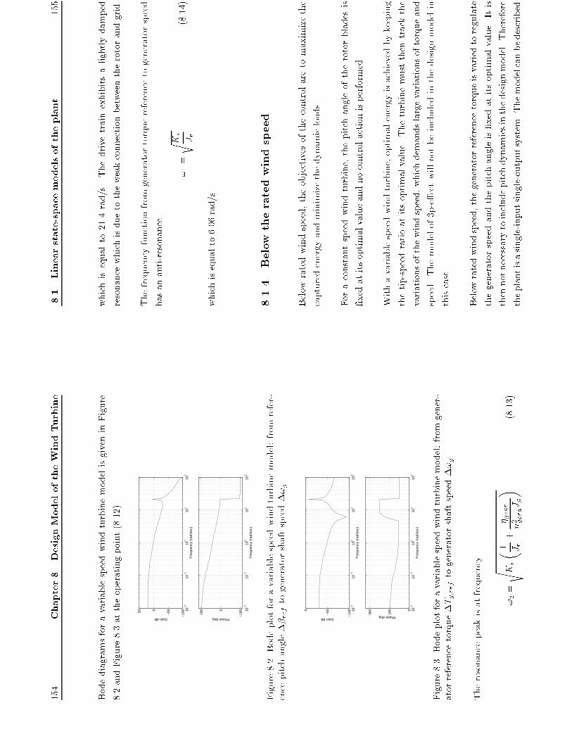
154

Chapter8.DesignModeloftheWindTurbine

BodediagramsforavariablespeedwindturbinemodelisgiveninFigure

8.2andFigure8.3attheoperatingpoint(8.12).

10−

210

−1

100

101

102

−10

0

−50050

Fre

quen

cy (

rad/

sec)

Gain dB

10−

210

−1

100

101

102

−18

00

180

Fre

quen

cy (

rad/

sec)

Phase deg

Figure8.2.Bodeplotforavariablespeedwindturbinemodel:fromrefer-

encepitchangle��reftogeneratorshaftspeed�!g.

10−

210

−1

100

101

102

−10

0

−500

Fre

quen

cy (

rad/

sec)

Gain dB

10−

210

−1

100

101

102

0

180

360

Fre

quen

cy (

rad/

sec)

Phase deg

Figure8.3.Bodeplotforavariablespeedwindturbinemodel:fromgener-

atorreferencetorque�Tg;reftogeneratorshaftspeed�!g.

Theresonancepeakisatfrequency

!2=

s Ks

� 1 Jr

+

�gear

n2 geraJg

�

(8.13)

8.1

Linearstate-spacemodelsoftheplant

155

whichisequalto21.4rad/s.Thedrivetrainexhibitsalightlydamped

resonancewhichisduetotheweakconnectionbetweentherotorandgrid.

Thefrequencyfunctionfromgeneratortorquereferencetogeneratorspeed

hasananti-resonance

!1=

r KsJr

(8.14)

whichisequalto6.06rad/s.

8.1.4

Below

theratedwindspeed

Belowratedwindspeed,theobjectivesofthecontrolaretomaximizethe

capturedenergyandminimizethedynamicloads.

Foraconstantspeedwindturbine,thepitchangleoftherotorbladesis

�xedatitsoptimalvalueandnocontrolactionisperformed.

Withavariablespeedwindturbine,optimalenergyisachievedbykeeping

thetip-speedratioatitsoptimalvalue.Theturbinemustthentrackthe

variationsofthewindspeed,whichdemandslargevariationsoftorqueand

speed.Themodelof3p-e�ectwillnotbeincludedinthedesignmodelin

thiscase.

Belowratedwindspeed,thegeneratorreferencetorqueisvariedtoregulate

thegeneratorspeedandthepitchangleis�xedatitsoptimalvalue.Itis

thennotnecessarytoincludepitchdynamicsinthedesignmodel.Therefore

theplantisasingle-inputsingle-outputsystem.Themodelcanbedescribed

156

Chapter8.DesignModeloftheWindTurbine

by

2 6 6 4�_ � �

�_!r

�_!g

3 7 7 5=2 6 6 40

1

�1ngear

�Ks

Jr

1 Jr

@Tw

@!r

0

�gearKs

ngearJg

0

0

3 7 7 52 6 6 4�� �

�!r

�!g

3 7 7 5

+2 6 6 40 0 �

1 Jg

3 7 7 5�Tg;ref+

2 6 6 40

1 Jr

@Tw

@v

0

3 7 7 5�v wind

(8.15)

andoutputequationsare

" �!g

�Tg

# =" 0

0

1

0

0

0#2 6 6 4�� �

�!r

�!g

3 7 7 5+" 0 1# �

Tg;ref

(8.16)

Themodelcanberepresentedby(8.11)withxp

=

[�� �;�!r;�!g]T,

u=�Tg;ref,y=[�!g;�Tg]TandLp2=0.

10−

310

−2

10−

110

010

110

2−

100

−500

Fre

quen

cy (

rad/

sec)

Gain dB

10−

310

−2

10−

110

010

110

20

180

360

Fre

quen

cy (

rad/

sec)

Phase deg

Figure8.4.Bodeplotforavariablespeedwindturbinemodel:fromgener-

atorreferencetorque�Tg;reftogeneratorshaftspeed�!g.

8.2

Noisemodels

157

Bodediagramisgivenforafrequencyfunctionfromgeneratortorqueref-

erencetogeneratorspeedinFigure8.4atanoperatingpoint

v m=7m=s

�opt=0:5o

!r;0=3:04rad=s

(8.17)

8.2

Noisemodels

Thewindmodelcanberepresentedbyasecondorderstate-spacemodel

" �_v wind

��v wind

# ="0

1

�1p1p2

�p1

+p2

p1p2

#"�v wind

�_v wind

# +"0 k

p1p2

# e w

�v wind=[10]" �

v wind

�_v wind

#

(8.18)

wheree wisazeromeanwhitenoisewithunitvariance.Ifthestateis

chosenasxw

=[�v wind�_v wind]T,theabovemodelcanbewrittenasa

noisemodel

_xw

=

Awxw

+Bwe w

�v wind

=

Cwxw

(8.19)

Inadesignmodelof3P-e�ect,theangularvelocityofrotorandrotortorque

shouldbeconsideredconstant,i.e.,!r=!r;0andTw

=Tw;0

�T3P(s)

e 3P(s)

=

k3PTw;0(3!r;0)2

s2+2�(3!r;0)s+(3!r;0)2

(8.20)

the3P-e�ectwillthenbemodelledbystate-spaceequations

" �_ T3P

�� T3P

# ="

0

1

�

(3!r;0)2

�

2�(3!r;0)

#"�T3P

�_ T3P

# +"

0

k3PTw;0(3!r;0)2

# e3P

158

Chapter8.DesignModeloftheWindTurbine

�T3P

=[10]" �

T3P

�_ T3P

#

(8.21)

whichinturncanberepresentedby

_x3P

=

A3Px3P

+B3Pe 3P

�T3P

=

C3Px3P

(8.22)

wheree 3P

isazeromeanwhitenoisewithunitvariance,anditisuncor-

relatedwithnoisesequencee w.The�T3P

modelcanonlybeincluded

inthedesignmodel,whentheangularvelocityofrotorcanbeconsidered

constant.Sincetherearesubstantialvariationsintherotorspeedwhena

variablespeedwindturbineisemployedbelowtheratedwindspeed,the

�T3P

modelwillnotbeincludedinthedesignmodelinthiscase.

8.3

A

compositemodel

Acompositemodelcanbebuiltinwhichtheplantmodel(8.11)andnoise

models(8.19)and(8.22)areuni�edintoonesinglestate-spacemodel

2 6 4_xp(t)

_xw(t)

_x3P(t)

3 7 5=2 6 4A

p

Lp1Cw

Lp2C3P

0

Aw

0

0

0

A3P

3 7 52 6 4xp(t)

xw(t)

x3P(t)

3 7 5

+2 6 4B

p 0 0

3 7 5u(t)+

2 6 40

0

Bw

0

0

B3P

3 7 5" ew(t)

e3P(t)

#(8.23)

y(t)=[Cp

0

0]2 6 4x

p(t)

xw(t)

x3P(t)

3 7 5+Dpu(t)

8.4

Discretetimemodel

159

Belowtheratedwindspeed,themodelof3P-e�ectwillbeomittedinthe

designmodel.

Ifwechoosex(t)=[xp(t)xw(t)x3P(t)]T

ande(t)=[ew(t)e 3P(t)]T,the

compositemodelcanberewrittenas

_x(t)

=

Acx(t)+Bcu(t)+Lce(t)

y(t)

=

Ccx(t)+Dcu(t)

(8.24)

Themainadvantageofstate-spacemodelisthataprioriknowledgeabout

thesysteminanaturalwaycanbeincludedinthemodel.Sincewehavea

well-knownphysicalstructureandphysicalmodelofthedrivetrainsystem,

themodelshouldbewellsuitedforthecontrollerdesignpurpose.

8.4

Discretetimemodel

Adigitalcontrollerisnormallyimplemented,whichsamplestheplantout-

putandcalculatesacontrolinputwhichis�xedduringthesampleperiod.

Inthissectionthesampleratewillbediscussedandthediscrete-timemodel

willbeformulated.

Generally,theperformanceofadigitalcontrollerimproveswithincreasing

samplerate,butcostmayalsobeincreasedwithfastersampling.The

selectionofthebestsamplerateforadigitalcontrolsystemisacompromise.

Thesamplingtheoremstatesthatinordertoreconstructanunknownband-

limitedcontinuoussignalfromsamplesofthatsignal,thesampleratemust

beatleasttwiceasfastasthehighestfrequencycontainedintheunknown

signal.Inpractice,thesignalwillneverbebandlimited,however,some

160

Chapter8.DesignModeloftheWindTurbine

frequencycontentsofthesignalcanbeconsideredinsigni�cantabovea

certainfrequency.

Basedonthesamplingtheorem,thesampleratedenotedbyf smustbeat

leasttwicetherequiredclosed-loopbandwidthofthesystemf b,i.e.,

f s f b>2

(8.25)

Thisisafundamentallowerboundonthesamplerate.

However,[Franklinetal.,1990]indicatesthatthetheoreticallowerbound

wouldbejudgedfartooslowforanacceptabletimeresponse.Hesuggests

thatthedesiredsamplingrateshouldbe

6�

f s f b�40

(8.26)

FortheconstantspeedWD34windturbine,thedrivetrainresonancefre-

quencyof6.13rad/s(�1Hz)isdominatedfrequency,asamplerateof10

HzinthecurrentusedPI-controllerhasbeenchosenbyVestas.Thissample

ratedwillalsobeusedinLQGcontrollerfortheconstantspeedpitchcon-

trolledwindturbineinordertomakeanunbiasedcomparison.However,for

avariablespeedpitchcontrolledwindturbine,duetoaverylightlydamped

resonanceatfrequencyof21.4rad/s(3.4Hz),asamplerateof33.33Hz(the

sampletimeis0.03s)ischosentoattenuatethedrivetrainresonance.

Thenacontinuousmodelcanbetransformedtoadiscrete-timemodel

x(t+1)

=

Adx(t)+Bdu(t)+w(t)

y(t)

=

Cdx(t)+Ddu(t)

(8.27)

8.5

Summary

161

8.5

Summary

Thedesignmodelsforwindturbineshavebeenderivedinthischapter.In

thecaseoffullload,modelsforaconstantspeedturbineandavariable

speedturbineareformulatedseparately.Inpartialload,onlyavariable

speedturbinewith�xedpitchismodelled.Boththewindmodelandthe

3P-e�ectareconsideredasnoisemodels.TheT3P

modelisincludedonlyin

fullload,inwhichtherearenotsigni�cantvariationsintherotorspeed.The

sampleratesfordigitalcontrolsystemsaredeterminedandageneralized

discrete-timestate-spacemodelisderived.

162

Chapter8.DesignModeloftheWindTurbine

Chapter9

EstimationofTheWind

Speed

Usingawindturbineforproductionofelectricalenergyrequiresreliableand

e�ectiveoperation,anactivecontrolsystemisoftenconsideredtorealizeit.

Somecontrolmethodsrequiretheknowledgeofthewindspeedexperienced

bytheturbine.Sincethenonlinearityoftheprocessfromtheaerodynamics

oftheturbinedependssigni�cantlyonthewindspeed,itseemsthatthe

windspeedisvitaltothebehaviourofclosed-loopsystem.

Althoughthereisnosuchthingasthewindspeedexperiencedbyawind

turbine,sincetherotorissubjecttoaspatiallydistributedwind�eldwhich

variesintime,theturbinemaybeconsideredtoexperienceane�ectivewind

speedwhichinsomesenseisanaverageovertherotordisc.Thismakes

163

164 Chapter 9. Estimation of The Wind Speed

a direct measurement of e�ective wind speed impossible. However, it is

also impossible to predict the true wind speed passing through the rotor

disc by measuring it by an anemometer, because the discrepancy between

the measured wind speed and true speed on the rotor is considerably large.

Even if it were possible, the presence of the turbine disturbs the wind speed

and the measurement would need to be made at separate site where the

wind speed correlated almost exactly with the wind speed experienced by

the turbine. Hence direct measurement of wind speed is of limited value

in regulating the wind turbine [Leithead et al., 1990]. The idea is then to

estimate the e�ective wind speed experienced by the rotor by using a wind

turbine as a wind measuring device.

Below the rated wind speed, the wind turbine will be adjusted to capture

as much as possible of the energy from the wind. If a tracking controller is

employed to keep the wind turbine running at optimal tip speed ratio where

the turbine can achieve maximumpower, the estimated wind speed is often

used to determine the optimal control action. In this case the accurate

estimated wind speed is a prerequisite for an appropriate control system

design. Above the rated wind speed, a controller can be used to smooth the

power generated by the wind turbine. If a gain scheduled LQG controller is

applied to compensate for nonlinearities of the process, the estimated wind

speed is often chosen as a scheduling variable to determine the operating

point where the controller can be calibrated each sample.

An input and output signal from the turbine are required by an estimator,

no matter which estimation method is used, see Figure 9.1. The plant

considered here is aWD34 constant speed wind turbine with PI pitch control

above rated wind speed and �xed pitch angle below rated wind speed. The

9.1 The Newton-Raphson method 165

v

Plant

Estimator

u y

^

Figure 9.1. Block scheme of estimator

input signal of the turbine is pitch demand and the output measurement is

electrical power.

In the following sections the Newton-Raphson method, Kalman �lter method

and extended Kalman �lter method will be developed for wind speed esti-

mation based on the model of the wind turbine. The performance of the

algorithms will be investigated by simulations. An identical wind sequence

is used for all simulations. Afterwards, some experimental data are used to

test the estimation approaches. An interesting discussion concerning wind

speed estimation is given at the end of chapter.

9.1 The Newton-Raphson method

The Newton type methods have been given in Appendix A. The reason to

use the Newton-Raphson method is that the method has particularly fast

convergence properties in most cases

[Dennis and Schnabel, 1983].

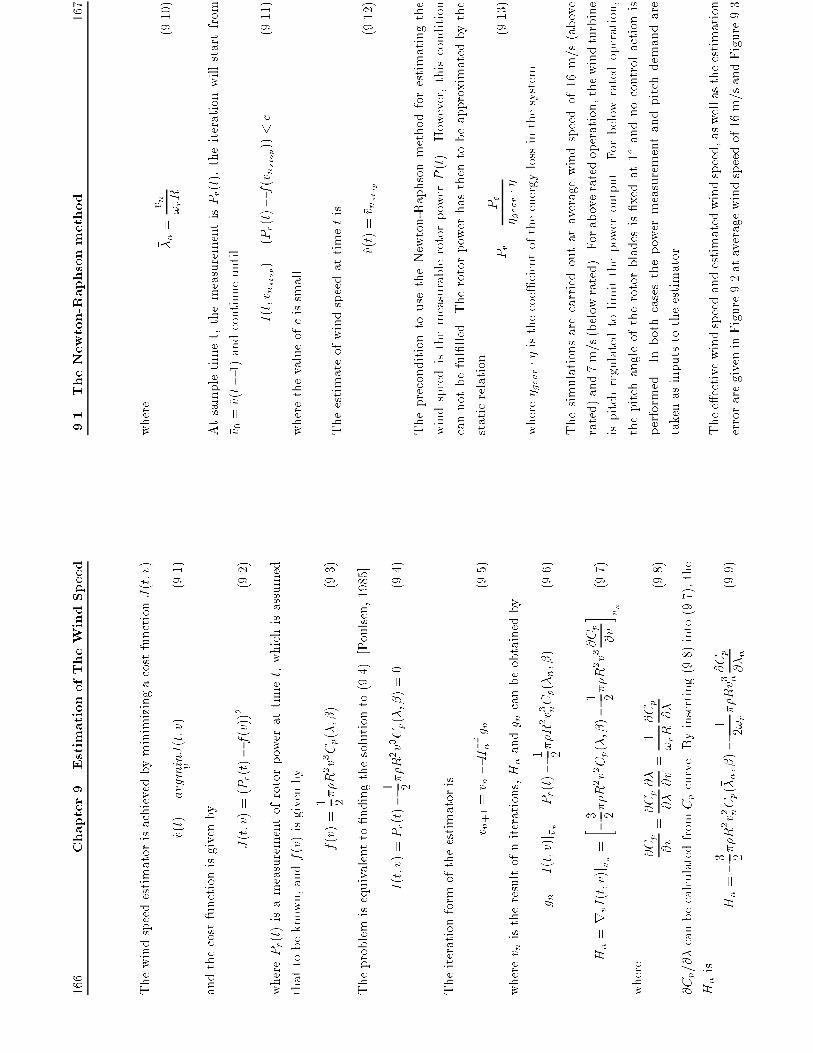
166

Chapter9.EstimationofTheWindSpeed

ThewindspeedestimatorisachievedbyminimizingacostfunctionJ(t;v)

^v(t)=argmin vJ(t;v)

(9.1)

andthecostfunctionisgivenby

J(t;v)=(Pr(t)�f(v))

2

(9.2)

wherePr(t)isameasurementofrotorpowerattimet,whichisassumed

thattobeknown,andf(v)isgivenby

f(v)=

1 2��R2v3Cp(�;�)

(9.3)

Theproblemisequivalentto�ndingthesolutionto(9.4)[Poulsen,1985]

I(t;v)=Pr(t)�

1 2��R2v3Cp(�;�)=0

(9.4)

Theiterationformoftheestimatoris

�v n+1=�v n�H�1n

g n

(9.5)

where�v nistheresultofniterations,Hnandg ncanbeobtainedby

g n=I(t;v)j �vn

=Pr(t)�

1 2��R2�v3 nCp(� �n;�)

(9.6)

Hn=r vI(t;v)j �vn

=� �3 2��R2v2Cp(�;�)�

1 2��R2v3@Cp

@v

� �vn

(9.7)

where

@Cp

@v

=@Cp

@�

@�

@v

=

1!rR

@Cp

@�

(9.8)

@Cp=@�canbecalculatedfromCpcurve.Byinserting(9.8)into(9.7),the

Hnis

Hn=�

3 2��R

2�v2 nCp(� �n;�)�

12!r

��R�v3 n

@Cp

@� �n

(9.9)

9.1

TheNewton-Raphsonmethod

167

where

� �n=

�v n !rR

(9.10)

Atsampletimet,themeasurementisPr(t),theiterationwillstartfrom

�v 0=^v(t�1)andcontinueuntil

I(t;�v nstop)=(Pr(t)�f(�vnstop))<c

(9.11)

wherethevalueofcissmall.

Theestimateofwindspeedattimetis

^v(t)=�v nstop

(9.12)

ThepreconditiontousetheNewton-Raphsonmethodforestimatingthe

windspeedisthemeasurablerotorpowerP(t).However,thiscondition

cannotbeful�lled.Therotorpowerhasthentobeapproximatedbythe

staticrelation

Pr=

Pe

�gear��

(9.13)

where�gear��isthecoe�cientoftheenergylossinthesystem.

Thesimulationsarecarriedoutataveragewindspeedof16m/s(above

rated)and7m/s(belowrated).Foraboveratedoperation,thewindturbine

ispitchregulatedtolimitthepoweroutput.Forbelowratedoperation,

thepitchangleoftherotorbladesis�xedat1oandnocontrolactionis

performed.Inbothcasesthepowermeasurementandpitchdemandare

takenasinputstotheestimator.

Thee�ectivewindspeedandestimatedwindspeed,aswellastheestimation

erroraregiveninFigure9.2ataveragewindspeedof16m/sandFigure9.3

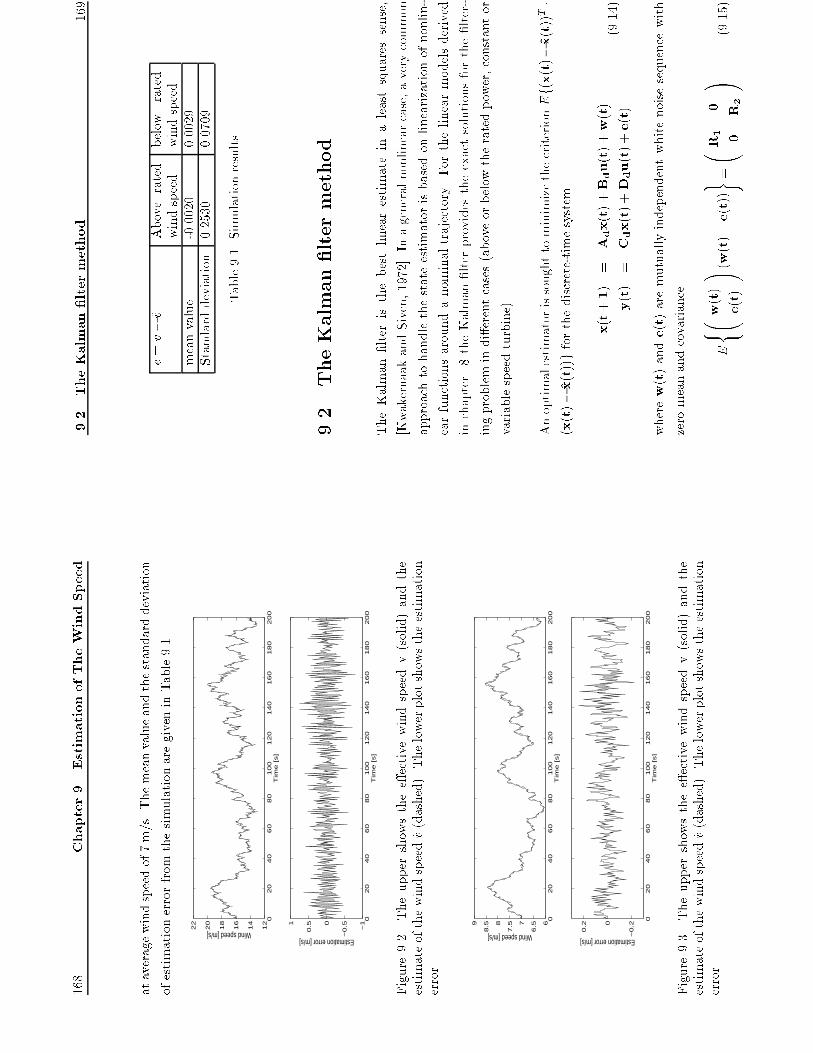
168

Chapter9.EstimationofTheWindSpeed

ataveragewindspeedof7m/s.Themeanvalueandthestandarddeviation

ofestimationerrorfromthesimulationaregiveninTable9.1.

02

04

06

08

01

00

12

01

40

16

01

80

20

01

2

14

16

18

20

22

Tim

e [s]

Wind speed [m/s]

02

04

06

08

01

00

12

01

40

16

01

80

20

0−

1

−0

.50

0.51

Tim

e [s]

Estimation error [m/s]

Figure9.2.Theuppershowsthee�ectivewindspeedv(solid)andthe

estimateofthewindspeed^v(dashed).Thelowerplotshowstheestimation

error

02

04

06

08

01

00

12

01

40

16

01

80

20

06

6.57

7.58

8.59

Tim

e [s]

Wind speed [m/s]

02

04

06

08

01

00

12

01

40

16

01

80

20

0

−0

.20

0.2

Tim

e [s]

Estimation error [m/s]

Figure9.3.Theuppershowsthee�ectivewindspeedv(solid)andthe

estimateofthewindspeed^v(dashed).Thelowerplotshowstheestimation

error

9.2

TheKalman�ltermethod

169

e=v�^v

Aboverated

windspeed

below

rated

windspeed

meanvalue

-0.0020

0.0029

Standarddeviation

0.2530

0.0709

Table9.1.Simulationresults

9.2

TheKalman�ltermethod

TheKalman�lteristhebestlinearestimateinaleastsquaressense,

[KwakernaakandSiven,1972].Inageneralnonlinearcase,averycommon

approachtohandlethestateestimatorisbasedonlinearizationofnonlin-

earfunctionsaroundanominaltrajectory.Forthelinearmodelsderived

inchapter8theKalman�lterprovidestheexactsolutionsforthe�lter-

ingproblemindi�erentcases(aboveorbelowtheratedpower,constantor

variablespeedturbine).

AnoptimalestimatorissoughttominimizethecriterionEf(x(t)�^x(t))T�

(x(t)�^x(t))gforthediscrete-timesystem

x(t+1)

=

Adx(t)+Bdu(t)+w(t)

y(t)

=

Cdx(t)+Ddu(t)+e(t)

(9.14)

wherew(t)ande(t)aremutuallyindependentwhitenoisesequencewith

zeromeanandcovariance

E( w(t)

e(t)

! (w(t)

e(t))

) = R

1

0

0

R2

!

(9.15)

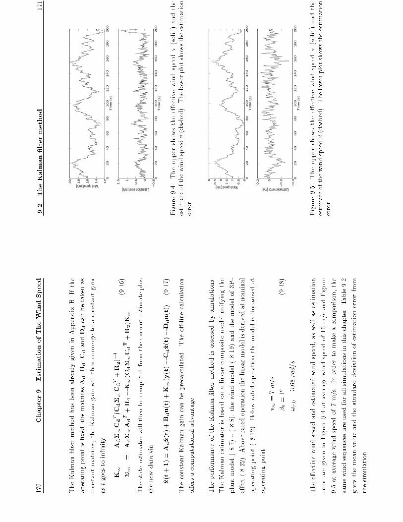
170

Chapter9.EstimationofTheWindSpeed

TheKalman�ltermethodhasbeenalreadygiveninAppendixB.Ifthe

operatingpointis�xed,thematricesAd,Bd,Cd

andDd

canbetakenas

constantmatrices,theKalmangainwillthenconvergetoaconstantgain

astgoestoin�nity.

K1

=

Ad�1Cd

T(Cd�1Cd

T+R2)�1

�1

=

Ad�1Ad

T+R1�K1(Cd�1Cd

T

+R2)K1

(9.16)

Thestateestimatorwillthenbecomputedfromthecurrentestimateplus

thenewdatavia

^x(t+1)=Ad^x(t)+Bdu(t)+K1(y(t)�Cd^x(t)�Ddu(t))

(9.17)

TheconstantKalmangaincanbeprecalculated.Theo�-linecalculation

o�ersacomputationaladvantage.

TheperformanceoftheKalman�ltermethodisassessedbysimulations.

TheKalmanestimatorisbasedonalinearcompositemodelunifyingthe

plantmodel(8.7)-(8.8),thewindmodel(8.19)andthemodelof3P-

e�ect(8.22).Aboveratedoperationthelinearmodelisderivedatnominal

operatingpoint(8.12).Belowratedoperationthemodelislinearizedat

operatingpoint

v m=7m=s

�0=1o

!r;0=3:68rad=s

(9.18)

Thee�ectivewindspeedandestimatedwindspeed,aswellasestimation

erroraregiveninFigure9.4ataveragewindspeedof16m/sandFigure

9.5ataveragewindspeedof7m/s.Inordertomakeacomparison,the

samewindsequencesareusedforallsimulationsinthischapter.Table9.2

givesthemeanvalueandthestandarddeviationofestimationerrorfrom

thesimulation.

9.2

TheKalman�ltermethod

171

02

04

06

08

01

00

12

01

40

16

01

80

20

01

2

14

16

18

20

Tim

e [s]

Wind speed [m/s]

02

04

06

08

01

00

12

01

40

16

01

80

20

0−

0.50

0.51

1.5

Tim

e [s]

Estimation error [m/s]

Figure9.4.Theuppershowsthee�ectivewindspeedv(solid)andthe

estimateofthewindspeed^v(dashed).Thelowerplotshowstheestimation

error

02

04

06

08

01

00

12

01

40

16

01

80

20

06

6.57

7.58

8.59

Tim

e [s]

Wind speed [m/s]

02

04

06

08

01

00

12

01

40

16

01

80

20

0−

0.4

−0

.20

0.2

Tim

e [s]

Estimation error [m/s]

Figure9.5.Theuppershowsthee�ectivewindspeedv(solid)andthe

estimateofthewindspeed^v(dashed).Thelowerplotshowstheestimation

error

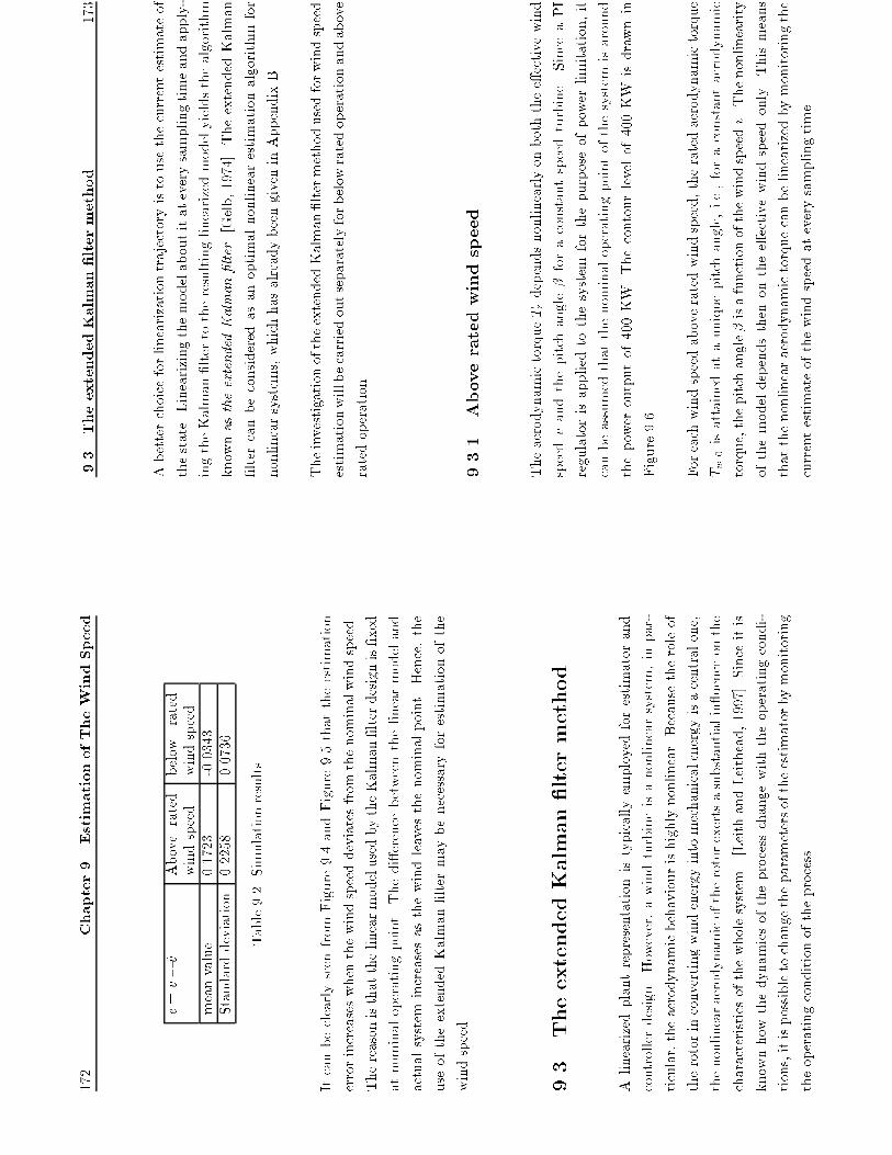
172

Chapter9.EstimationofTheWindSpeed

e=v�^v

Aboverated

windspeed

below

rated

windspeed

meanvalue

0.1723

-0.0343

Standarddeviation

0.2258

0.0736

Table9.2.Simulationresults

ItcanbeclearlyseenfromFigure9.4andFigure9.5thattheestimation

errorincreaseswhenthewindspeeddeviatesfromthenominalwindspeed.

ThereasonisthatthelinearmodelusedbytheKalman�lterdesignis�xed

atnominaloperatingpoint.Thedi�erencebetweenthelinearmodeland

actualsystemincreasesasthewindleavesthenominalpoint.Hence,the

useoftheextendedKalman�ltermaybenecessaryforestimationofthe

windspeed.

9.3

TheextendedKalman�ltermethod

Alinearizedplantrepresentationistypicallyemployedforestimatorand

controllerdesign.However,awindturbineisanonlinearsystem,inpar-

ticular,theaerodynamicbehaviourishighlynonlinear.Becausetheroleof

therotorinconvertingwindenergyintomechanicalenergyisacentralone,

thenonlinearaerodynamicoftherotorexertsasubstantialin uenceonthe

characteristicsofthewholesystem.[LeithandLeithead,1997].Sinceitis

knownhowthedynamicsoftheprocesschangewiththeoperatingcondi-

tions,itispossibletochangetheparametersoftheestimatorbymonitoring

theoperatingconditionoftheprocess.

9.3

TheextendedKalman�ltermethod

173

Abetterchoiceforlinearizationtrajectoryistousethecurrentestimateof

thestate.Linearizingthemodelaboutitateverysamplingtimeandapply-

ingtheKalman�ltertotheresultinglinearizedmodelyieldsthealgorithm

knownastheextendedKalman�lter[Gelb,1974].TheextendedKalman

�ltercanbeconsideredasanoptimalnonlinearestimationalgorithmfor

nonlinearsystems,whichhasalreadybeengiveninAppendixB.

TheinvestigationoftheextendedKalman�ltermethodusedforwindspeed

estimationwillbecarriedoutseparatelyforbelowratedoperationandabove

ratedoperation.

9.3.1

Aboveratedwindspeed

TheaerodynamictorqueTrdependsnonlinearlyonboththee�ectivewind

speedvandthepitchangle�foraconstantspeedturbine.SinceaPI

regulatorisappliedtothesystem

forthepurposeofpowerlimitation,it

canbeassumedthatthenominaloperatingpointofthesystemisaround

thepoweroutputof400KW.Thecontourlevelof400KW

isdrawnin

Figure9.6.

Foreachwindspeedaboveratedwindspeed,theratedaerodynamictorque

Tw;0isattainedatauniquepitchangle,i.e.,foraconstantaerodynamic

torque,thepitchangle�isafunctionofthewindspeedv.Thenonlinearity

ofthemodeldependsthenonthee�ectivewindspeedonly.Thismeans

thatthenonlinearaerodynamictorquecanbelinearizedbymonitoringthe

currentestimateofthewindspeedateverysamplingtime.

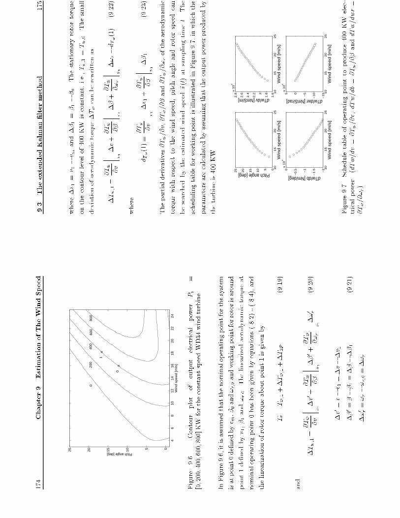
174

Chapter9.EstimationofTheWindSpeed

46

81

01

21

41

61

82

02

22

4

05

10

15

20

25

Win

d s

pe

ed

[m

/s]

Pitch angle [deg]

02

00

40

06

00

80

0

o

o

0

1

Figure

9.6.

Contour

plot

of

output

electrical

power

Pe

=

[0;200;400;600;800]KW

fortheconstantspeedWD34windturbine.

InFigure9.6,itisassumedthatthenominaloperatingpointforthesystem

isatpoint0de�nedbyv m,�0and!r;0andworkingpointforrotorisaround

point1de�nedbyv 1,�1and!r;0.Thelinearizedaerodynamictorqueat

nominaloperatingpoint0hasbeengivenbyequations(8.2)-(8.4),and

thelinearizationofrotortorqueaboutpoint1isgivenby

Tr=Tw;1+�Tw;1+�T3P

(9.19)

and

�Tw;1=

@Tw@v

? ? ? ? v 1�v0 +@Tw@�

? ? ? ? v 1��0 +@Tw

@!r

? ? ? ? v 1�!0 r

(9.20)

�v0 =v�v 1=�v��v 1

��0 =���1=�����1

(9.21)

�!0 r=!r�!r;0=�!r

9.3

TheextendedKalman�ltermethod

175

where�v 1=v 1�v mand��1=�1��0.Thestationaryrotortorque

onthecontourlevelof400KW

isconstant,i.e.,Tw;1=Tw;0.Thesmall

deviationofaerodynamictorque�Tw

canberewrittenas

�Tw;1=

@Tw@v

? ? ? ? v 1�v+

@Tw@�

? ? ? ? v 1��+

@Tw

@!r

? ? ? ? v 1�!r�dTw

(1)

(9.22)

where

dTw

(1)=

@Tw@v

? ? ? ? v 1�v 1+

@Tw@�

? ? ? ? v 1��1

(9.23)

Thepartialderivatives@Tw=@v,@Tw=@�and@Tw=@!roftheaerodynamic

torquewithrespecttothewindspeed,pitchangleandrotorspeedcan

besearchedbytheestimatedwindspeed^v(t)atsamplingtimet.The

schedulingtableforworkingpointisillustratedinFigure9.7,inwhichthe

parametersarecalculatedbyassumingthattheoutputpowerproducedby

theturbineis400KW.

10

15

20

25

05

10

15

20

25

Win

d s

pe

ed

[m

/s]

Pitch angle [deg]

10

15

20

25

1.6

1.82

2.2

2.4

2.6

2.8

x 1

04

Win

d s

pe

ed

[m

/s]

dTw/dv [NmS/m]

10

15

20

25

−2

−1

.5−1

−0

.50x 1

04

Win

d s

pe

ed

[m

/s]

dTw/db [Nm/deg]

10

15

20

25

−1

5

−1

0

−505

x 1

04

Win

d s

pe

ed

[m

/s]

dTw/dwr [NmS/rad]

Figure9.7.Scheduletableofoperatingpointtoproduce400KW

elec-

tricalpower.(dTw=dv=@Tw=@v,dTw=db=@Tw=@�anddTw=dwr=

@Tw=@!r)

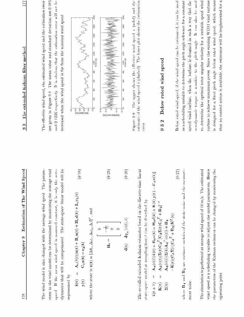
176

Chapter9.EstimationofTheWindSpeed

Thewindmodelisalsochangedwiththeaveragewindspeed.Theparam-

etersinthewindmodelcanbedeterminedbymonitoringtheaveragewind

speed.Ifthemeanwindspeedisassumedconstant,itisonlytheaero-

dynamicsthatwillbecompensated.Thestate-spacelinearmodelwillbe

representedby

_x(t)

=

Ac(^v(t))x(t)+Bcu(t)+Hcd(t)+Lce1(t)

y(t)

=

Ccx(t)+e2(t)

(9.24)

wherethestateisx(t)=[�� �;�!r;�!g;��]T,and

Hc=

2 6 6 6 6 40 �

1 Jr

0 0

3 7 7 7 7 5

(9.25)

d(t)=dTw

(^v(t);t)

(9.26)

Theso-calledextendedKalmanestimatorbasedonthediscrete-timelinear

state-spacemodelatsamplingtimetcanbedescribedby

^x(t+1)

=

Ad(^v(t))^x(t)+Bdu(t)+Hdd(t)+K(t)[y(t)�Cdx(t)]

K(t)

=

Ad(^v(t))�(t)Cd

T[Cd�(t)Cd

T+R2]�1

�(t)

=

Ad(^v(t))�(t)Ad

T(^v(t))+R1

�K(t)(Cd�(t)Cd

T+R2)KT(t)

(9.27)

whereR1

andR2

arevariancemetricsofthestatenoiseandthemeasure-

mentnoise.

Thesimulationisperformedataveragewindspeedof16m/s.Theestimated

windspeedisaschedulingvariabletoadjustthemodelparameters.Hence

theparametersoftheKalmanestimatorcanbechangedbymonitoringthe

operatingpoint.

9.3

TheextendedKalman�ltermethod

177

Thee�ectivewindspeed,theestimatedwindspeedandtheestimationerror

aregiveninFigure9.8.Themeanvalueandstandarddeviationare0.085

and0.1236respectively.Itisobviousthattheestimationerrorwillnotbe

increasedwhenthewindspeedisfarfromthenominalwindspeed.

02

04

06

08

01

00

12

01

40

16

01

80

20

01

2

14

16

18

20

22

Tim

e [s]

Wind speed [m/s]

02

04

06

08

01

00

12

01

40

16

01

80

20

0−

0.4

−0

.20

0.2

0.4

Tim

e [s]

Estimation error [m/s]

Figure9.8.Theuppershowsthee�ectivewindspeedv(solid)andthe

estimateofthewindspeed^v(dashed).Thelowerplotshowstheestimation

error

9.3.2

Below

ratedwindspeed

Belowratedwindspeed,ifthewindspeedcanbeestimated,itcanbeused

asaschedulingvariabletodeterminethepitchanglereferenceforaconstant

speedwindturbine,whentheturbineisdesignedinsuchawaythatthe

aerodynamictorqueissensitivetothepitchangle.Itcanalsobeused

todeterminetheoptimalrotorangularvelocityforavariablespeedwind

turbinetoachievemaximumpower.SincetheexistingWD34windturbine

isdesignedfora�xedpitchanglebelowratedwindspeed,whichmeans

thatnocontrolactionisavailable,theestimatorwillbeimplementedfora

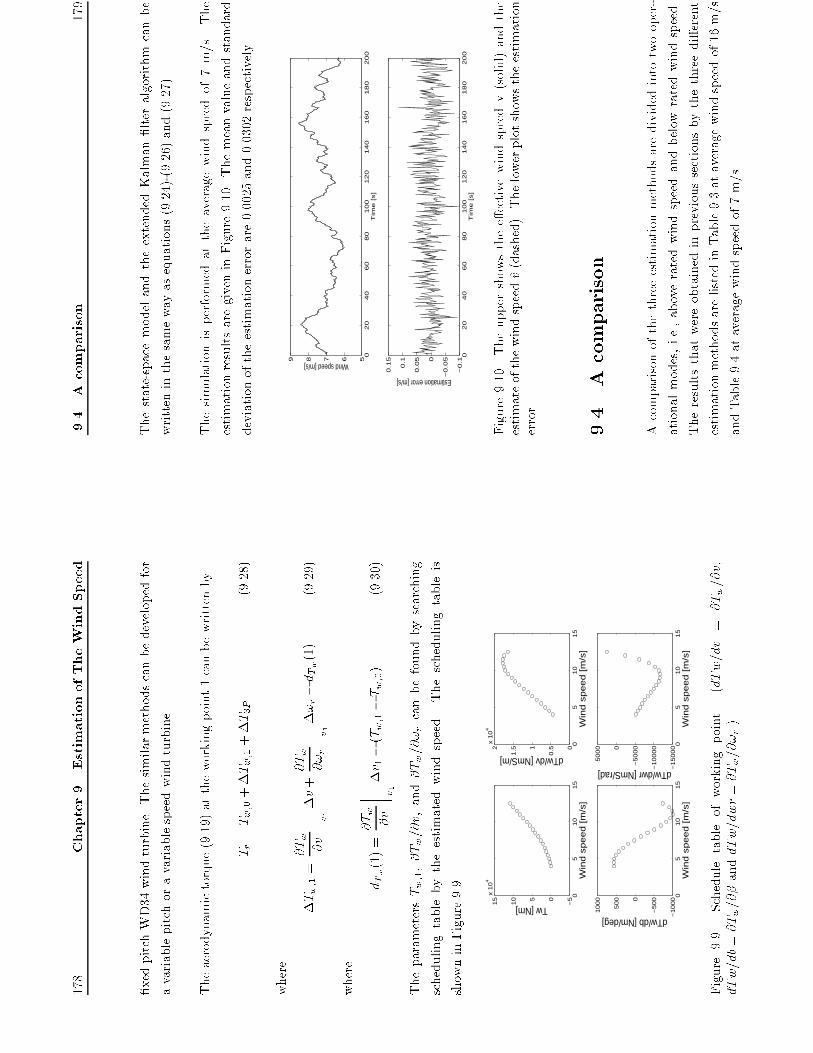
178

Chapter9.EstimationofTheWindSpeed

�xedpitchWD34windturbine.Thesimilarmethodscanbedevelopedfor

avariablepitchoravariablespeedwindturbine.

Theaerodynamictorque(9.19)attheworkingpoint1canbewrittenby

Tr=Tw;0+�Tw;1+�T3P

(9.28)

where

�Tw;1=

@Tw@v

? ? ? ? v 1�v+

@Tw

@!r

? ? ? ? v 1�!r�dTw

(1)

(9.29)

where

dTw

(1)=

@Tw@v

? ? ? ? v 1�v 1�(Tw;1�Tw;0)

(9.30)

TheparametersTw;1,@Tw=@v,and@Tw=@!r

canbefoundbysearching

schedulingtablebytheestimatedwindspeed.Theschedulingtableis

showninFigure9.9.

05

10

15

−505

10

15

x 1

04

Win

d s

pe

ed

[m

/s]

Tw [Nm]

05

10

15

0

0.51

1.52

x 1

04

Win

d s

pe

ed

[m

/s]

dTw/dv [NmS/m]

05

10

15

−1

00

0

−5

000

50

0

10

00

Win

d s

pe

ed

[m

/s]

dTw/db [Nm/deg]

05

10

15

−1

50

00

−1

00

00

−5

00

00

50

00

Win

d s

pe

ed

[m

/s]

dTw/dwr [NmS/rad]

Figure9.9.

Scheduletableofworkingpoint.

(dTw=dv

=

@Tw=@v,

dTw=db=@Tw=@�anddTw=dwr=@Tw=@!r.)

9.4

A

comparison

179

Thestate-spacemodelandtheextendedKalman�lteralgorithmcanbe

writteninthesamewayasequations(9.24)-(9.26)and(9.27).

Thesimulationisperformedattheaveragewindspeedof7m/s.The

estimationresultsaregiveninFigure9.10.Themeanvalueandstandard

deviationoftheestimationerrorare0.0025and0.0302respectively.

02

04

06

08

01

00

12

01

40

16

01

80

20

056789

Tim

e [s]

Wind speed [m/s]

02

04

06

08

01

00

12

01

40

16

01

80

20

0−

0.1

−0

.050

0.0

5

0.1

0.1

5

Tim

e [s]

Estimation error [m/s]

Figure9.10.Theuppershowsthee�ectivewindspeedv(solid)andthe

estimateofthewindspeed^v(dashed).Thelowerplotshowstheestimation

error

9.4

A

comparison

Acomparisonofthethreeestimationmethodsaredividedintotwooper-

ationalmodes,i.e.,aboveratedwindspeedandbelowratedwindspeed.

Theresultsthatwereobtainedinprevioussectionsbythethreedi�erent

estimationmethodsarelistedinTable9.3ataveragewindspeedof16m/s

andTable9.4ataveragewindspeedof7m/s.

180

Chapter9.EstimationofTheWindSpeed

e=v�^v

Newton

Kalman

Extended

Kalman

meanvalue

-0.0020

0.1723

0.0142

Standarddeviation

0.2530

0.2258

0.1236

Table9.3.Ataveragewindspeedof16m/s.

e=v�^v

Newton

Kalman

Extended

Kalman

meanvalue

-0.0029

-0.0343

0.0025

Standarddeviation

0.0709

0.0736

0.0302

Table9.4.Ataveragewindspeedof7m/s.

TheNewton-RaphsonmethodwiththeassumptionPr=Pe=�providesa

smallmeanvalueofestimationerrorinbothcases,butitgivesalarge

variance.ThereasonisthattherotorpowerPrisnotmeasurableandthe

assumptionPr=Pe=�leadstotheestimationerror.However,theNewton-

Raphsonmethodisthemostsimplemethod.Itisnotbasedonthemodel

ofthewholesystemanditisnotnecessarytoknowtheaveragewindspeed.

TheKalman�ltermethodgivesbothlargevarianceandmeanvalueof

estimationerrorinthethreemethods,becausethelinearmodelusedinthe

Kalman�lterdesignis�xedatnominaloperatingpoint.Itcanbeclearly

seenfromthesimulations,theestimationerrorisincreasedwhenthewind

speeddeviatesfromthenominalwindspeed,wherethedi�erencebetween

thelinearmodelandactualsystemincreases.TheKalman�lteralgorithm

yieldsless�lteringaccuracythantheextendedKalman�lteralgorithm,

9.5

Test

181

butito�erscomputationaladvantage.TheKalmangaincanbecalculated

o�-line.

TheextendedKalman�lterisaspecialkindofopen-loopadaptationor

changeofestimatorparameters,whichgivesthebestperformanceinthe

threemethods.Themethodachievesthesmallestvariancesinbothcases.

TheextendedKalman�ltermethodhastheadvantagethatthelinearmodel

usedintheKalman�lterdesigncanbecalibratedforoperatingpointby

monitoringtheestimatedwindspeed.Thereforethechangesinprocess

gaincanbeconsideredbytheestimator,andtheestimationerrorwillnot

beincreasedwhenthewindspeeddeviatesfromthenominalwindspeed.

BoththeKalman�ltermethodandtheextendedKalman�ltermethod

requireagoodmodelofthesystem.EventhoughtheextendedKalman

�ltergivesthebestperformance,becauseofthecomputationtimerequired

bythemethodandlimitedavailableresources,theNewtonandKalman

�ltermethodsarestillgoodchoicesforimplementationonarealturbine.

9.5

Test

ThedatasequencesfromtheWD34windturbinewerecollectedinanopen-

loopexperiment,inwhichthepitchangleofrotorbladeswas�xedat1o,the

windspeedandpoweroutputweremeasured.Thewindwasmeasuredby

ananemometerwhichisat68minfrontoftheturbine,atthesameheight

asthehub.

182 Chapter 9. Estimation of The Wind Speed

A comparison of the experimental data and the estimated data is very dif-

�cult. First of all, the measured wind speed has to be �ltered to obtain the

wind speed experienced by the rotor. The �lter function is an approxima-

tion. Secondly, the distance between the measurement point and rotor of

the turbine may cause a time delay and discrepancy between the measured

wind speed and the true wind speed at the wind turbine, especially the high

frequency components in the wind. Thirdly, the power measurements are

corrupted by 1P, 2P and 3P- uctuations, which have to be �ltered out. The

model of 3P-e�ect is not included in the design model in this test.

Pitch angle

filterLP

Comparison

Wind

measurements

Effective

wind speed

EstimatorEstimated

wind speed

Filtered power

measurements

Figure 9.11. Block scheme of the comparison

The block scheme of the comparison of the experimental result and esti-

mated wind speed is illustrated in Figure 9.11. The e�ective wind speed

experienced by the turbine is derived by dynamically �ltering the measure-

ments of the point wind speed. The �lter function was given in ( 7.45). The

pitch angle and power measurements will be used as an input and output

signal to the estimator. Since there are evident contents of 1P, 2P and 3P-

e�ect in the power measurements, which depend signi�cantly on the speci�c

wind turbine and site, the power measurements have to be �ltered by band-

stop �lters with bandwidth of 0:15�(n!r;0) and a fourth order Butterworth

low-pass �lter with cut-o� frequency of 8 rad/s to discard high frequency

9.5 Test 183

components. The block scheme of pre�ltering the power measurements is

shown in Figure 9.12.

measurements

Power

measurementsfilter1P

filter2P

filter3P

filterLP Filtered power

Figure 9.12. Pre�ltering of power measurements

The test is carried out by using the Kalman �lter method. The simulation

result is plotted in Figure 9.13. The estimated wind speed given in the �gure

seems to agree with the �ltered measurements. The time delay between the

estimated wind speed and �ltered wind measurements can be obviously

seen. This is caused by the distance between the measurement point and

the turbine. The two data sequences deviate in some areas, it may caused

by the distance or the precision of the �lter function.

0 50 100 150 200 250 3004.5

5

5.5

6

6.5

7

7.5

8

Time [s]Wi

nd sp

eed [

m/s]

Figure 9.13. The �ltered measurements v (solid) and the estimate of the

wind speed ^v (dashed)

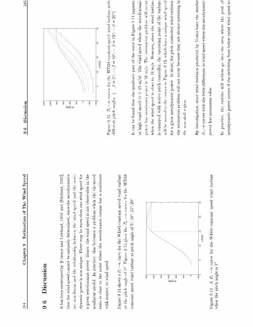
184

Chapter9.EstimationofTheWindSpeed

9.6

Discussion

Ithasbeenmentionedby[ConnorandLeithead,1994]and[Ekelund,1997],

thatthewindspeedcannotbeuniquelydetermined,sincetheaerodynamics

arenon-linearandtherelationshipbetweenthewindspeedandtheaero-

dynamicpowerisnon-unique:Theremaybemorethanonewindspeedfor

agivenaerodynamicpower.Hence,thewindspeedisnotobservableinthe

nonlinearmodel.Inpractice,thisbecomesaproblemwhenthetip-speed

ratioisclosetothepointwheretheaerodynamictorquehasamaximum

withrespecttowindspeed.

Figure9.14showsaPr�vcurvefortheWD34constantspeedwindturbine

atthepitchangleof1o.Figure9.15givesthePr�vcurvesfortheWD34

constantspeedwindturbineatpitchangleof5o;10o;15o;20o.

05

10

15

20

25

−1

000

10

0

20

0

30

0

40

0

50

0

60

0

v [m

/s]

Pr [KW]

Figure9.14.APr�vcurvefortheWD34constantspeedwindturbine

whenthepitchangleis1o.

9.6

Discussion

185

05

10

15

20

25

−4

00

−2

000

20

0

40

0

60

0

80

0

10

00

12

00

v [m

/s]

Pr [KW]

Figure9.15.Pr�vcurvesfortheWD34constantspeedwindturbinewith

di�erentpitchangles.(|

�=5o;--�=10o;-��=15o;���=20o)

ItcanbefoundthatthequadraticpartofthecurveinFigure9.14appears

athighwindspeed(v>15m/s).Thewindspeedwheretheaerodynamic

powerhasmaximumpoweris18m/s.Theestimationproblemwilloccur

whenthewindspeediscloseto18m/s.However,sincethewindturbine

isequippedwithactivepitchcontroller,theoperatingpointoftheturbine

willbemovedtothecurvesinFigure9.15,whichhaveauniquewindspeed

foragivenaerodynamicpower.Inshort,forpitchcontrolledwindturbines

theestimationproblemwillnotoccurbecausetheyarealwaysoperatingin

thenon-stallregion.

Byinvestigation,mostwindturbinesproducedbyVestashavethesimilar

Pr�vcurveswiththelittledi�erencesinwindspeedwheretheaerodynamic

powerhasmaximumvalue.

Inpractice,theturbinewillseldom

gointotheareawherethepeakof

aerodynamicpoweroccursiftheswitchingfrombelowratedwindspeedto

186

Chapter9.EstimationofTheWindSpeed

aboveratedwindspeedorverseviceareproperlydesigned.Inorderto

increasetherobustnessofthecontroller,theoperatingpointclosedtothe

switchingpointcanbe�xedforthecontroller,andgainschedulingwith

theestimatedwindspeedasaschedulingvariablewillonlybeimplemented

whenthepitchislargerthan5o.

Asithasbeensuggestedby

[Ekelund,1997],analternativeapproachis

tode�netheoperationalstrategyinthetorque-rotorspeedplane.Any

controlstrategyisequivalenttoacurveinthisplane.Onlyanestimateof

aerodynamictorqueisrequiredratherthananestimateofwindspeed.

9.7

Summary

Threedi�erentestimationmethodshavebeenpresentedinthissection.An

analysisandcomparisonofthreemethodsaremadebasedonthesimulation

results.Theestimationmethodsaretestedbyexperimentaldata,andthe

estimatedwindspeedshowsagoodagreementwiththe�lteredmeasure-

mentsofthepointwindspeed.Theresultsindicatethatestimationofthe

windspeedisausefulmethodforthecontrollerdesign,ifitrequiresthe

knowledgeofthewindspeed.However,theproblemmayoccuratswitching

area,whichrequirecarefullydesignoftheswitchingfromaboveratedwind

speedtobelowratedwindspeedorversevice.

Chapter10

ControlAboveRated

Power

Theemphasisofthischapterisgiventothedesignofcontrolsystemsabove

ratedpower.Designofcontrolsystemsforaconstantspeedandvariable

speedwindturbineistreatedseparately.

Thecontrolobjectivesforwindturbinesoutlinedintheintroductionneed

tobeclari�edmoreprecisely.Theloadtransientsexperiencedbythewind

turbineareoftwotypes.Firstly,thewind,asadisturbanceinputtothetur-

bine,resultsinlargeoscillationsindrivetraintorqueandelectricalpower.

Thecontrolsystemshouldattempttoreducethesetoaminimumandre-

ducethestressonthepowertraincomponents.Variationsinloadscannot

becompletelyeliminatedbutreducingtheirmagnitudeisdesirable.To

187

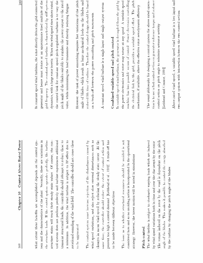
188

Chapter10.ControlAboveRatedPower

whatextentthesebene�tsareaccomplisheddependsonthecontrolsys-

temandthecharacteristicsoftheplant.Secondly,therearevariationsin

thestructureloads.Ifthecontrolsystem

operatesperfectly,theturbine

structurestateswilltracktheirsteadystatevalues.Ofcourse,thecon-

trolsystemdoesnotperformperfectlyandturbineexperiencesadditional

transientstructuralloads,thecontrollershouldattempttoreducetheseto

aminimum.Inaddition,thewindturbineissubjectto3P-e�ectdueto

rotationalsamplingofthewind�eld.Thecontrollershouldnotcausethese

tobeaggravated.

Thecontrolsystemmustincreaserejectionofthedisturbancescausedby

windspeedvariations,andalsorejectslowexternaldisturbancessuchas

changesinmeanwindspeedbyreducingthesteadystateerrors.Atthe

sametime,thecontrollershouldreducetheextentofcontrolactionand

preventtoohighacontroldemand[Leitheadetal.,1992].Atrade-o�has

tobemadebetweendi�erentobjectives.

Theissueastowhetherstructuralresonancesshouldbeavoidedisnot

consideredhereandsonoavoidingactionisincorporatedintheoperational

strategy.However,thetowermotionwillbenotedinsimulations.

Pitchcontrol

Thewindturbineissubjecttostochasticvaryingloadswhichareinduced

bywindspeedvariationsbothintimeandoverthediscsweptbytherotor.

Thetorqueinducedontherotorbythewindisdependentonthepitch

angleoftheblades.Thismakesitpossibletocontroltheenergyabsorbed

bytheturbinebychangingthepitchangleoftheblades.

189

Inconstantspeedwindturbines,therotordirectlydrivesthegrid-connected

generatorandhencemustrotateatanapproximate�xedmultipleofthe

gridfrequency.Theconstantspeedturbineischaracterizedbysti�system

dynamics,withalargerotorinertia.Whenthewindspeedrisesaboverated,

thecontroltaskforconstantspeedpitch-regulatedturbinesistovarythe

pitchangleofthebladessuitablytoregulatethepoweroutputtotherated

value,whileminimizingtheloadtransientsandtherebyreducingfatigue.

However,thetaskofpowersmoothingrequiresfastvariationsofthepitch

angleofbladeswhichresultinlargemechanicalloadsonthebladesand

reducedlifetimeofturbines.Thereforethecontroldesignshouldbebased

onatrade-o�betweenthepowersmoothingandpitchmovements.

Aconstantspeedwindturbineisasingleinputandsingleoutputsystem.

Combinedvariablespeedandpitchcontrol

Invariablespeedwindturbines,thegeneratorisdecoupledfromthegridby

thepowerelectronicsandrotormayrotateatanyspeed.Avariablespeed

machinehastwopossiblemeansofcontrol.Powerelectronicscontrolling

theelectricallinktothegrid,providesavariablespeede�ect.Thepitch

mechanism,ifavailable,altersthee�ectiverotoraerodynamice�ciency.

Theusualphilosophyfordesigningacontrolsystemforaboveratedopera-

tionistouseafastcontrolactionongeneratorreferencetorqueandaslower

controlactiononpitchangletominimizeactuatoractivity.

[LeitheadandConnor,1994]

Aboveratedwindspeed,avariablespeedwindturbineisatwoinputand

twooutputsystemwithinteractionbetweenthetwocontrolactions.

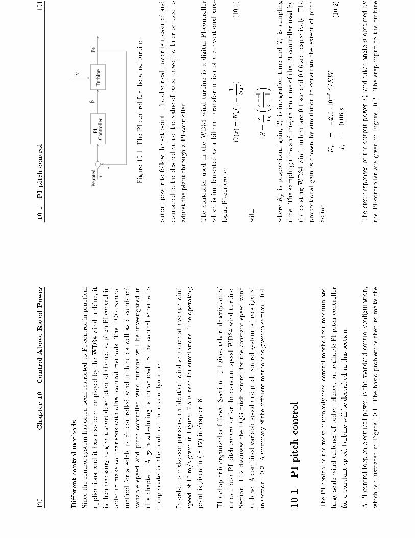
190

Chapter10.ControlAboveRatedPower

Di�erentcontrolmethods

SincethecontrolsystemhasoftenbeenrestrictedtoPIcontrolinpractical

applications,andithasalsobeenemployedbytheWD34windturbine,it

isthennecessarytogiveashortdescriptionoftheactivepitchPIcontrolin

ordertomakecomparisonswithothercontrolmethods.TheLQGcontrol

methodforasolelypitchcontrolledwindturbineaswellasacombined

variablespeedandpitchcontrolledwindturbinewillbeinvestigatedin

thischapter.Againschedulingisintroducedtothecontrolschemeto

compensateforthenonlinearrotoraerodynamics.

Inordertomakecomparisons,anidenticalwindsequenceataveragewind

speedof16m/sgiveninFigure7.5isusedforsimulations.Theoperating

pointisgivenin(8.12)inchapter8.

Thischapterisorganizedasfollows.Section10.1givesashortdescriptionof

anavailablePIpitchcontrollerfortheconstantspeedWD34windturbine.

Section

10.2discussestheLQGpitchcontrolfortheconstantspeedwind

turbine.Acombinedvariablespeedandpitchcontrolsystemisinvestigated

insection10.3.Asummaryofthedi�erentmethodsisgiveninsection10.4.

10.1

PIpitchcontrol

ThePIcontrolisthemostcommonlyusedcontrolmethodformediumand

largescalewindturbinesoftoday.Hence,anavailablePIpitchcontroller

foraconstantspeedturbinewillbedescribedinthissection.

APIcontrollooponelectricalpoweristhestandardcontrolcon�guration,

whichisillustratedinFigure10.1.Thebasicproblemisthentomakethe

10.1

PIpitchcontrol

191

-

Pe,r

ated

PIC

ontr

olle

rT

urbi

nev

Peβ

+

Figure10.1.ThePIcontrolforthewindturbine

outputpowertofollowthesetpoint.Theelectricalpowerismeasuredand

comparedtothedesiredvalue(thevalueofratedpower)witherrorusedto

adjusttheplantthroughaPI-controller.

ThecontrollerusedintheWD34windturbineisadigitalPI-controller

whichisimplementedasabilineartransformationofaconventionalana-

loguePI-controller

G(z)=Kp(1+

1STi

)

(10.1)

with

S=

2 Ts

� z�1

z+1

�

whereKp

isproportionalgain,TiisintegrationtimeandTsissampling

time.ThesamplingtimeandintegrationtimeofthePIcontrollerusedby

theexistingWD34windturbineare0.1secand0.06secrespectively.The

proportionalgainischosenbysimulationtoconstraintheextentofpitch

action.

Kp

=

�2:9�10�6o=KW

Ti

=

0:06s

(10.2)

ThestepresponsesoftheoutputpowerPeandpitchangle�obtainedby

thePI-controlleraregiveninFigure10.2.Thestepinputtotheturbine

192

Chapter10.ControlAboveRatedPower

isthewindspeedwhichchangesfrom16m/sto17m/sat1sec.Itcan

beseenthattheoutputpowerissuppressedbythePIpitchregulatorto

followthepowerreference.However,theovershootoftheoutputpoweris

large,whichisalmostofsameamplitudeastheuncontrolledsystem.The

3P-e�ectisnotincludedinsimulationmodelinordertoshowthesteady

stateresponses.

01

23

45

67

89

10

35

0

40

0

45

0

50

0

55

0

Tim

e [s]

Power [KW]

01

23

45

67

89

10

12

12

.513

13

.514

14

.515

Tim

e [s]

Pitch angle [deg]

Figure10.2.StepresponsesofoutputpowerandpitchanglewithPI-

controller.Thedashedlineintheupperplotisopen-loopresponseofoutput

power.

Thebodeplotsofthetransferfunctionfromthewindtotheoutputpower

forthecontrolledanduncontrolledwindturbinearegiveinFigure10.3.

The�gureshowsthatthePI-controllerattenuatesthevariationsinthe

electricalpowercausedbythewindvariationsuptoabout1.7rad/s.How-

ever,between1.7rad/sand7.5rad/sthevariationsareincreased,which

isundesirable.Itcanbefoundthatthe3Presonanceatthefrequencyof

11rad/sisneitherattenuatednorampli�ed,but1Presonanceatfrequency

of3.685rad/sisampli�ed.Thereisaslightincreaseinamplitudeatthe

structuralresonancefrequencyof6.9rad/s.Simulationshowsthatthese

slightincreaseisnotharmful.

10.1

PIpitchcontrol

193

10

01

01

70

80

90

10

0

11

0

Fre

qu

en

cy [ra

d/s

]

Gain [dB]

Figure10.3.Bodeplotsofthetransferfunctionfrom

�vto�Pe.The

dashedlineisfortheopen-loopsystemandthesolidlineisfortheclosed

loopsystemwithPI-controller.

ThePI-controllerisfurthermoredesignedwithanonlineargainscheduling.

Thenonlinearityreducesthegainwithincreasingpitchtocompensatefor

theincreaseingainthroughthesystem.

Toobtainamorerealisticevaluationofthecontrollerthefullnon-linear

stochasticmodelofthewindturbineisemployedforsimulation.ThePI-

regulatorgivenin(10.1)-(10.1)isimplementedforpowerlimitation.The

resultsareshowninFigure10.4,inwhichacomparisonbetweenthepower

outputfrom

theopen-loopsystem

andtheclosed-loopsystem

showsthe

performanceofthePI-regulator.Thepitchangleofbladesisalsoplotted

inthe�gure.

Itisobviousthatthein uenceofthedisturbancesfromthewindonthe

outputpowerisreducedbythecontroller,i.e.,thecontrollerenhancesthe

disturbancerejectionpropertiesoftheturbineandsmooththegenerated

power.

194

Chapter10.ControlAboveRatedPower

50

60

70

80

90

10

01

10

12

01

30

14

01

50

10

0

20

0

30

0

40

0

50

0

60

0

70

0

tim

e [

s]

Pe [KW]

50

60

70

80

90

10

01

10

12

01

30

14

01

50

5

10

15

20

tim

e [

s]

Pitch angle [deg]

Figure10.4.SimulationofthewindturbinewithaPI-controller.Theupper

plotshowsthepoweroutputfromtheuncontrolled(dashed)andcontrolled

(solid)windturbine.Thelowerplotshowsthepitchangleoftheblades.

Thekeyparametersfromthesimulationof200secaregiveninTable10.1.

Theoutputpowerandgeneratorreactiontorqueareusedasanindicatorof

theperformanceofclosed-loopsystem.Thepitchangleandpitchrateare

giventoshowthepitchperformancesincetherearestrictlimitsonthemin

ordertopreventthecontrolactionfrombeingtoostrong.Thespeedand

displacementoftowerbendingmovementaregiventoseeifthecontroller

excitesthetowerbending.

BycomparingtheparametersinTable10.1withTable7.2obtainedfroman

open-loopsimulation,itcanbefoundthatthestandarddeviationofgenera-

torreactiontorquehasbeendecreasedsigni�cantlybythePI-controller,i.e.,

theloadtransientsthroughouttheturbinehavebeenalleviatedandsmooth

powercanthusbeachieved.ItcanalsobefoundthatthePI-controllerdoes

notgivethesigni�cantincreasesinthetowerbendingmovements.

10.2

LQG

pitchcontrol

195

mean(Pe)[KW]

mean(Tg)[Nm]

mean(!g)[rad/s]

max(ht!t)[cm/s]

399.46

3928.83

105.77

2.59

SD(Pe)[KW]

SD(Tg)[Nm]

SD(!g)[rad/s]

max(ht�t)[cm]

34.92

340.20

0.09

3.65

max(�)[deg]

min(�)[deg]

SD(�)

max(_ �)[deg/s]

19.65

3.88

3.55

5.04

Table10.1.StatisticsobtainedwhilesimulatingthePIpitchcontrolsystem.

Meanwindspeedis16m/s.

However,ithasbeenmentionedby[Leithead,1989a]thatthePI-controller

maynotbeentirelysatisfactorybecauseitisunabletoadddamping.

10.2

LQG

pitchcontrol

LQG

optimalcontrollaw

LinearQuadraticGaussian(LQG)optimalcontrollawis�rmlyestablished

basedonstate-spacedescriptionofsystems.Themaincharacteristicsof

LQGareoptimizationintermsofquadraticperformancecriteriaandincor-

porationoftheKalmanoptimalestimationtheory

[Bitmeadetal.,1990].

Figure10.5depictstheinterconnectionoftheplant,theobserverandthe

controllawforapitchregulatedwindturbine.

Thequadraticcostfunctionwhichweseektominimizeisgivenby

J(N;t)=E

8 < :N�1 X j

=0

fQy(�Pe(t+j))2+Qu(��ref(t+j))2g9 = ;(10.3)

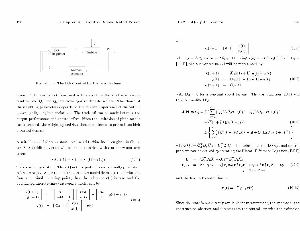
196 Chapter 10. Control Above Rated Power

Turbine

v

RegulatorLQ

Kalmanestimator

^

Peβ

x

Figure 10.5. The LQG control for the wind turbine

where E denotes expectation used with respect to the stochastic uncer-

tainties, and Qy and Qu are non-negative de�nite scalars. The choice of

the weighting parameters depends on the relative importance of the output

power quality or pitch variations. The trade-o� can be made between the

output performance and control e�ect. Since the limitation of pitch rate is

easily reached, the weighting matrices should be chosen to prevent too high

a control demand.

A suitable model for a constant speed wind turbine has been given in Chap-

ter 8. An additional state will be included to deal with stationary non-zero

errors

xi(t+ 1) = xi(t) + (r(t)� y(t)) (10.4)

This is an integral state. The r(t) in the equation is an externally prescribed

reference signal. Since the linear state-space model describes the deviations

from a nominal operating point, then the reference r(t) is zero and the

augmented discrete-time state-space model will be"x(t+ 1)

xi(t + 1)#

=

"Ad 0

�Cd I#"x(t)

xi(t)#

+"Bd

0

#u(t) +w(t)

y(t) = [ Cd 0 ]"x(t)

xi(t)#

+ e(t)

(10.5)

10.2 LQG pitch control 197

and

xi(t+ 1) = [ 0 I ]"x(t)

xi(t)#

(10.6)

where y = �Pe and u = ��ref . Denoting �x(t) = [x(t) xi(t)]T and Ci =

[ 0 I ], the augmented model will be represented by

�x(t+ 1) = �Ad�x(t) + �Bdu(t) +w(t)

y(t) = �Cd�x(t) + �Ddu(t) + e(t)

xi(t+ 1) = Ci�x(t)

(10.7)

with �Dd = 0 for a constant speed turbine. The cost function (10.3) will

then be modi�ed by

J(N;x(t)) = EfN�1X

j=0fQy(�Pe(t+ j))2 + Qu(��ref (t + j))2

+xTi (t+ j)Qixi(t+ j)gg (10.8)

= E8<

:N�1X

j=0f�xT(t+ j)Qx�x(t+ j) +Qu(��ref (t+ j))2g

9=;

where Qx = �CTdQy�Cd +CTi QiCi. The solution of the LQ optimal control

problem can be derived by iterating the Riccati Di�erence Equation (RDE)

Lj = (�BTdPj�Bd +Qu)�1 �BTdPj�Ad

Pj+1 = �ATdPj�Ad �

�ATdPj�Bd(�BTdPj�Bd +Qu)�1 �BTdPj�Ad +Qx

j = 0; � � �N � 1

(10.9)

and the feedback control law isu(t) = ��LN�1�x(t) (10.10)

Since the state is not directly available for measurement, the approach is to

construct an observer and interconnect the control law with the estimated

198 Chapter 10. Control Above Rated Power

state

u(t) = �[L Li]"^x(t)

^xi(t)#

(10.11)

The Kalman estimation method given in section 9.2 can be used to estimate

the state.

The control strategy with di�erent weights on the the pitch reference is

illustrated by the step responses in Figure 10.6. The step input to the

turbine is wind speed which changes from 16 m/s to 17 m/s at 1 sec.

0 1 2 3 4 5 6 7 8 9 10300

350

400

450

500

550

Time [s]

Powe

r [KW

]

0 1 2 3 4 5 6 7 8 9 1012

13

14

15

16

Time [s]

Pitc

h an

gle

[deg

]

Figure 10.6. Step responses of output power Pe and pitch angle � obtained

by LQG controller with di�erent weight on pitch reference. Qy = 1, Qu =

4:3 � 1011 (|), 20 � 1011 (- -), 1010 (-�). The dotted line in the upper plot is

the power output in open-loop.

With high weight on the control action the turbine follows the power ref-

erence slowly (dashed line). However, the large control action excites the

tower bending movements and leads to the vibrations on pitch control action

and turbine dynamics (dash-dot line). In practice, the large pitch action

is not allowed to avoid heavy mechanical loads. A compromise is made

10.2 LQG pitch control 199

between power smoothing and load alleviation by choosing Qy = 1 and

Qu = 4:3 �1011. The step response with these weighting parameters is given

by the solid line. It can be found that the output power has been sup-

pressed and the amplitude of overshoot is decreased by the LQG regulator

compared to the PI-controller with the similar pitch action.

Gain scheduling

An e�ective control algorithm must re ect both the plant dynamic char-

acteristics as well as the anticipated working environment. The control

problem is therefore divided into two time scales corresponding to slow mean

wind speed changes and rapid turbulent wind speed variations. Changes in

mean wind speed cause the mean pitch angle of the blade to alter to main-

tain the mean power output at its rated value. These mean pitch positions

are treated as steady state operating points, which can be determined by

searching scheduling table 9.7 with the average wind speed obtained by

�ltering the measured point wind speed through a low-pass �lter with a

period of 10 minutes.

Regulator Process+Reference

Gainschedule

ParamtersRegulator

conditionOperating

yu

-

Figure 10.7. Block diagram of a gain scheduling system

Secondly, the aerodynamic behaviour is highly nonlinear. When a linear

representation of rotor aerodynamic torque is employed, the partial deriva-

tives @Tw=@v, @Tw=@� and @Tw=@!r of the aerodynamic torque with respect

200

Chapter10.ControlAboveRatedPower

towindspeed,pitchangleandrotorspeedareactuallytime-varyingand

dependontheoperatingconditions.Sincewehaveknownhowtherotor

aerodynamicschangewiththeoperatingconditionsoftheprocess,itis

thenpossibletochangetheparametersofthecontrollerbymonitoringthe

operatingconditions.Thisiscalledgainscheduling.Theprincipleofgain

schedulingisillustratedinFigure10.7.Thegainschedulinghasalinearreg-

ulatorwhoseparametersarechangedasafunctionofoperatingconditions

inanopen-loopfashion.

Forawindturbine,theestimatedwindspeedortheaveragewindspeed

canbeusedasschedulingvariablestomonitortheoperatingconditionsof

theprocess.TheschedulingtableisplottedinFigure9.7inChapter9.

Theparameters@Tw=@v,@Tw=@�and@Tw=@!rinthelinearaerodynamic

torquemodelcanbefoundbysearchingschedulingtablewiththeestimated

windspeedorthemeanwindspeedateachsample.Thismeansthatthe

linearmodelusedinestimatorandregulatoriscalibratedforeachoperating

pointandthenonlinearaerodynamicscanthenbecompensated.

Simulationresults

SimulationiscarriedoutatthesameoperatingpointasthePI-controller,

andthesamewindsequenceisusedforthesimulation.Thesimulation

resultscanthusbecomparedwiththeresultsobtainedbyusingthePI-

controller.Inordertomakecomparisons,thesimilarcontrolactionsare

requiredandmaximumvalueofthepitchrateislimitedtoabout5o=sfor

boththePIandtheLQGcontrol.TheLQGcontrollerwithweighting

parametersQy

=

1andQu

=

4:3�1011

isperformed,whichgivesthe

similarpitchactionasthePI-controllerdoes.Thegainschedulingisnot

implementedinthisexample.

10.2

LQG

pitchcontrol

201

ThesimulationresultsareshowninFigure10.8,andkeyparametersfrom

thesimulationaregiveninTable10.2.

50

60

70

80

90

10

01

10

12

01

30

14

01

50

10

0

20

0

30

0

40

0

50

0

60

0

70

0

Tim

e [

s]

Pe [KW]

50

60

70

80

90

10

01

10

12

01

30

14

01

50

5

10

15

20

Tim

e [

s]

Pitch angle [deg]

Figure10.8.SimulationofthewindturbinewithaLQG-controller.The

upperplotshowsthepoweroutputfrom

theuncontrolled(dashed)and

controlled(solid)windturbine.Thelowerplotshowsthepitchangleofthe

blades.

mean(Pe)[KW]

mean(Tg)[Nm]

mean(!g)[rad/s]

max(ht!t)[cm]

399.16

3927.07

105.77

3.74

SD(Pe)[KW]

SD(Tg)[Nm]

SD(!g)[rad/s]

max(ht�t)[cm]

24.75

241.11

0.06

3.45

max(�)[deg]

min(�)[deg]

SD(�)

max(_ �)[deg/s]

19.43

5.03

3.34

5.05

Table10.2.StatisticsobtainedwhilesimulatingtheLQG

pitchcontrol

system.Meanwindspeedis16m/s.

202 Chapter 10. Control Above Rated Power

It can be found that the standard deviation of output power is reduced

by the LQG controller compared to the PI-controller. This corresponds to

the decrease of the variations in generator reaction torque. By keeping the

generator torque variations small, the shaft loads are reduced and thereby

the turbine life will be increased. As the PI-controller, the LQG controller

does not give the signi�cant increases in tower bending movements.

10.3 Combined variable speed and pitch con-

trol

The purpose of this section is to investigate the control system of a variable

speed wind turbine which employs pitch regulation and generator reaction

torque regulation in high wind speeds.

Turbine

v

RegulatorLQ

Kalmanestimator

y

x̂

u

Figure 10.9. The LQG control for the wind turbine

Variable speed pitch regulation presents a multivariable control problem as

an additional generator torque control loop is added to the existing pitch

control loop. The ability to vary the rotor speed of a wind turbine increases

the operational exibility. Figure 10.9 shows the block scheme of combined

10.3 Combined variable speed and pitch control 203

variable speed and pitch control of a wind turbine by implementing the

LQG control method.

The dynamics of the generator and frequency converter have been discussed

in section 7.6. The linear design model for a variable speed wind turbine

given in Chapter 8 has the pitch reference and generator torque reference

as inputs and the angular velocity and reaction torque of the generator as

outputs

u ="��ref

�Tg;ref#

y ="�!g

�Tg#

(10.12)

The model is augmented by including integral actions to give zero steady-

state errors. The model can be represented by ( 10.7). The performance

criterion is speed wind turbine

J(N;x(t)) = EfN�1X

j=0fyT(t+ j)Qyy(t+ j)

+uT(t+ j)Quu(t+ j) + xTi (t+ j)Qixi(t+ j)gg (10.13)

= EfN�1X

j=0f�xT(t+ j)Qx�x(t+ j) + 2�xT(t+ j)Qxuu(t+ j)

+uT(t+ j)Q0uu(t+ j)gg (10.14)

where matrices Qx = �CTdQy�Cd + CTi QiCi, Qxu = �CTdQy�Dd and Q0u =

�DTdQy�Dd +Qu, and

Qy ="qy1 0

0 qy2#

Qu ="qu1 0

0 qu2#

Qi ="qi1 0

0 qi2#

(10.15)

The choice of the weighting matrices Qy and Qu depend on the relative

importance of the output power quality or input restrictions. qu1 and qu2

in matrix Qu can be chosen such that the the pitch position and pitch rate

should be restricted and the rotor speed will be remained within prede�ned

limitation. Qi will be chosen to punish the stationary error.

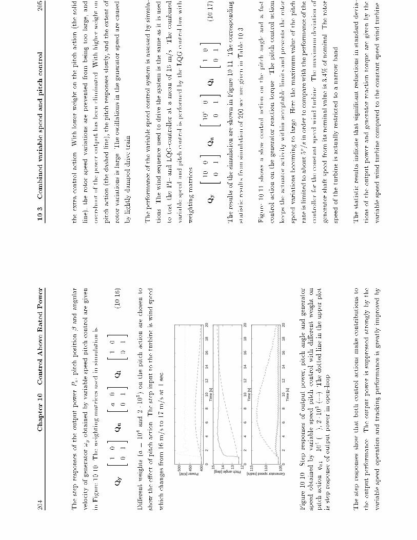
204

Chapter10.ControlAboveRatedPower

ThestepresponsesoftheoutputpowerPe,pitchposition�andangular

velocityofgenerator!gobtainedbyvariablespeedpitchcontrolaregiven

inFigure10.10.Theweightingmatricesusedinsimulationis

Qy

=" 1

0

0

1#

Qu

=" a0

0

1#

Qi=

" 1

0

0

1#

(10.16)

Di�erentweights(a=104and2�105)onthepitchactionarechosento

showthee�ectofpitchaction.Thestepinputtotheturbineiswindspeed

whichchangesfrom16m/sto17m/sat1sec.

02

46

810

1214

1618

2040

0

450

500

Tim

e [s

]

Power [KW]

02

46

810

1214

1618

2012131415

Tim

e [s

]

Pitch angle [deg]

02

46

810

1214

1618

2010

5

110

115

Tim

e [s

]

Generator speed [rad/s]

Figure10.10.Stepresponsesofoutputpower,pitchangleandgenerator

speedobtainedbyvariablespeedpitchcontrolwithdi�erentweighton

pitchaction.q u1=104(|),2�105(--).Thedottedlineintheupperplot

isstepresponseofoutputpowerinopen-loop.

Thestepresponsesshowthatbothcontrolactionsmakecontributionsto

theoutputperformance.Theoutputpowerissuppressedstronglybythe

variablespeedoperationandtrackingperformanceisgreatlyimprovedby

10.3

Combinedvariablespeedandpitchcontrol

205

theextracontrolaction.Withlowerweightonthepitchaction(thesolid

line),therotorspeedvariationsarepreventedfrom

beingtoolarge,and

overshootofthepoweroutputhasbeeneliminated.Withhigherweighton

pitchaction(thedashedline),thepitchresponsesslowly,andtheextentof

rotorvariationsislarge.Theoscillationsinthegeneratorspeedarecaused

bylightlydampeddrivetrain.

Theperformanceofthevariablespeedcontrolsystemisassessedbysimula-

tions.Thewindsequenceusedtodrivethesystemisthesameasitisused

totestthePI-andLQG-controlleratameanof16m/s.Thecombined

variablespeedandpitchcontrolisperformedbytheLQGcontrollawwith

weightingmatrices

Qy

=" 10

0

0

1#

Qu

=" 104

0

0

1#

Qi=

" 1

0

0

1#

(10.17)

TheresultsofthesimulationareshowninFigure10.11.Thecorresponding

statisticresultsfromsimulationof200secaregiveninTable10.3.

Figure10.11showsaslowcontrolactiononthepitchangleandafast

controlactiononthegeneratorreactiontorque.Thepitchcontrolaction

keepstheactuatoractivitywithinacceptablelimitsandpreventstherotor

speedvariationsbecomingtolarge.Herethemaximumvalueofthepitch

rateislimitedtoabout5o=sinordertocomparewiththeperformanceofthe

controllerfortheconstantspeedwindturbine.Themaximumdeviationof

generatorshaftspeedfromitsnominalvalueis3:4%ofnominal.Therotor

speedoftheturbineisactuallyrestrictedtoanarrowband.

Thestatisticresultsindicatethatsigni�cantreductionsinstandarddevia-

tionsoftheoutputpowerandgeneratorreactiontorquearegivenbythe

variablespeedwindturbinecomparedtotheconstantspeedwindturbine.

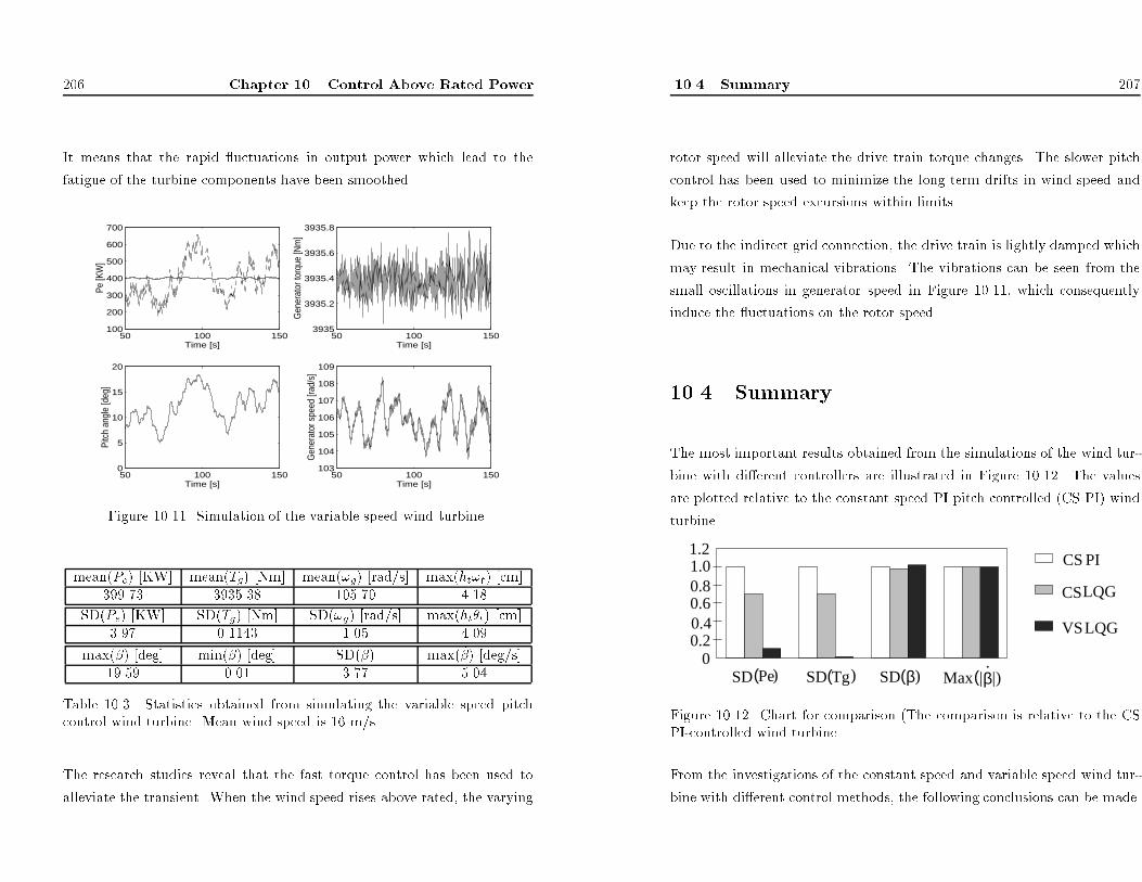
206 Chapter 10. Control Above Rated Power

It means that the rapid uctuations in output power which lead to the

fatigue of the turbine components have been smoothed.

50 100 150100

200

300

400

500

600

700

Time [s]

Pe [K

W]

50 100 1500

5

10

15

20

Time [s]

Pitc

h an

gle

[deg

]

50 100 1503935

3935.2

3935.4

3935.6

3935.8

Time [s]

Gen

erat

or to

rque

[Nm

]

50 100 150103

104

105

106

107

108

109

Time [s]

Gen

erat

or s

peed

[rad

/s]

Figure 10.11. Simulation of the variable speed wind turbine.

mean(Pe) [KW] mean(Tg) [Nm] mean(!g) [rad/s] max(ht!t) [cm]

399.73 3935.38 105.70 4.18

SD(Pe) [KW] SD(Tg) [Nm] SD(!g) [rad/s] max(ht�t) [cm]

3.97 0.1143 1.05 4.09

max(�) [deg] min(�) [deg] SD(�) max( _�) [deg/s]

19.59 0.01 3.77 5.04

Table 10.3. Statistics obtained from simulating the variable speed pitch

control wind turbine. Mean wind speed is 16 m/s.

The research studies reveal that the fast torque control has been used to

alleviate the transient. When the wind speed rises above rated, the varying

10.4 Summary 207

rotor speed will alleviate the drive train torque changes. The slower pitch

control has been used to minimize the long term drifts in wind speed and

keep the rotor speed excursions within limits.

Due to the indirect grid connection, the drive train is lightly damped which

may result in mechanical vibrations. The vibrations can be seen from the

small oscillations in generator speed in Figure 10.11, which consequently

induce the uctuations on the rotor speed.

10.4 Summary

The most important results obtained from the simulations of the wind tur-

bine with di�erent controllers are illustrated in Figure 10.12. The values

are plotted relative to the constant speed PI pitch controlled (CS PI) wind

turbine.

0.20.4

0.81.0

0.6

1.2

CS

0MaxSD(β) |β|)(

.(SD Pe) (SD Tg)

CS PI

LQG

VSLQG

Figure 10.12. Chart for comparison (The comparison is relative to the CS

PI-controlled wind turbine.

From the investigations of the constant speed and variable speed wind tur-

bine with di�erent control methods, the following conclusions can be made.

208

Chapter10.ControlAboveRatedPower

ThePIpitchcontrolisstillafavouredmeansofregulationforconstant

speedwindturbinesbecauseofthesimplicityofthemethod.

TheLQGpitchcontrolachievesasigni�cantreductionintheextentofthe

transientsofdrivetrainloadandhencesmoothesthepower.Theinvestiga-

tionsindicatethattheLQGcontrolismoreappropriatethanthePIcontrol.

However,thesimulationresultsarebasedonanaccuratemodelwhichmay

notalwaysbeobtainedinpractice.FortheLQGcontrolmethod,astate

estimatormustbeemployedinanypracticalimplementation.

Foravariablespeedwindturbine,thesystemtobecontrolledismultivari-

ablewithinputsbeingthereferencegeneratortorqueandpitchdemandand

outputsbeingthegeneratorreactiontorqueandgeneratorspeed.Consid-

erableimprovedperformanceisprovidedbyperformingtheLQGvariable

speedpitchcontrol.Theabilitytooperateatvariablerotorspeede�ec-

tivelyaddscompliancetothepowertraindynamicsofthewindturbine

andachievesamoregentlepitchmotionregime.Thepitchactioninvari-

ablespeedoperationisusedtopreventtherotorspeedvariationsfrombeing

toolarge.Therotorspeedisactuallyfreetovarywithinasmallinterval.

Thecombinedvariablespeedpitchcontrolcanalsoberealizedbyusing

thePIcontrolmethod.Twocontrolloopswiththepitchreferenceand

generatortorquereferenceasinputswillbeincludedinthecontrolscheme.

ThePImultivariablecontrolisnotdiscussedinthisthesis.

Anotheradvantageofthevariablespeedoperationisthatrotorspeedcan

beadjustedtoreducenoiselevelsandhencemakethewindturbinemore

environmentallyagreeable,becausethenoiselevelproducedbywindturbine

isafunctionoftherotorspeed.

10.4

Summary

209

Thebene�tsofusingvariablespeedwindturbinemustbeo�setagainst

thedisadvantages:themoreexpensivegeneratorsystemduetotheintro-

ductionofpowerconversiondeviceandreducedreliabilityofthevariable

speedelectricalmachinery.However,itisanticipatedthatthecostofpower

conversiondevicewilldecreaseastechnologyadvances.

Aswindspeedrises,fora�xedcontrollerthestandarddeviationofthe

poweroutputalsorisesduetotheincreasedlevelofturbulence.Itisthere-

foreattractivetoincreasethecontrolleractivitybyapplyinggainscheduling

methodwhichgivesimproveddisturbancerejection.Thegainscheduling

methodisinanopen-loopfashion,thepossiblyoccurredsteadystateerrors

ofoperatingpointscanbeeliminatedbytheintegralactions.

210

Chapter10.ControlAboveRatedPower

Chapter11

ControlBelowRated

Power

Itwasmentionedpreviouslythatthewindturbineoperationwasdivided

intotworegions,i.e.,aboveratedwindspeedandbelowratedwindspeed.

Sinceawindturbinespendsmostofitslifeoperatinginwindspeedsless

thanrated,itseemsmoreimportanttoinvestigatetheroleande�ectsof

controlsystemsinpartialload.

Belowratedwindspeedthecontrolstrategyistomaximizeenergycapture

fromthewindandminimizetheturbinetransientloads.Inpartialload

itistheaerodynamicpowerthatshouldbemaximized,sincetheenergyis

capturedbytherotor.However,theoverallproductionofelectricalenergy

isimproved,sincethecapturedenergyisonlytemporarilystoredinrotor.

211

212

Chapter11.ControlBelowRatedPower

TherotorcharacteristicsofawindturbinearesummarizedbytheCpsur-

face,wherethepowercoe�cientCp(�;�)de�ningtheabilityoftheturbine

toconvertthekineticenergyofthewindtomechanicalenergycapturedby

therotorisanonlinearfunctionofpitchangle�andtipspeedratio�.In

ordertomaximizetheenergycapture,thesetwovariablesshouldbekept

attheiroptimalvaluestoachievethemaximumvalueofCp.Thepitch

anglecanbeeasily�xedattheoptimalvalue.However,sincethetipspeed

ratiode�nedby�=v=(!rR)isa�ectedbythewindspeedexperienced

bytheturbineandtherotorspeed,therotorspeedistheonlywaywhich

canberegulatedtoachievetheoptimal�.Hence,avariablespeedturbine

isrequiredtotrackthevariationsofwindspeedandhencemaximizethe

aerodynamicpower.

00.

10.

20.

30.

40

0.1

0.2

0.3

0.4

0.5

λ

Cp

Cp,

max

λop

t

Figure11.1.Cp(�)-curveatpitchangleof0:5o

ACp(�;�0)-curveoftheWD34windturbineatoptimalpitchangleof

�0=0:5oisshowninFigure11.1.Therotordevelopsmaximummechanical

poweronlyatspeci�ctip-speedratio�opt.Iftherotorspeedisheldcon-

stant,theoperatingpointvariesontheCp(�)-curvefromcut-intorated

windspeed,resultinginreducede�ciency.Ontheotherhand,ifrotor

213

speedisallowedtovary,itcantrackthewindvelocitytokeepthetip-speed

ratioatitsoptimumvalue.

Sincethesensitivityoftheaerodynamictorquetothechangeofthepitch

angleisloweratlowwindspeeds,nocontrolactiononthepitchanglewill

thenberequirednormally.

Withthepitchangleatitsoptimalvalue,thecontrolobjectiveistomaxi-

mizethepowercoe�cientatallwindspeedsbykeepingthetipspeedatits

optimalvalue.Ontheotherhand,thecontrolobjectiveisalsooptimized

withrespecttotheminimizationoftheturbinetransientloads.Obviously,

thetwoobjectivesmentionedabovecontradicteachother.Inordertokeep

thetipspeedratioconstant,therotorspeedmustexactlyfollowthewind

turbulence,whichrequireslargevariationsinrotorspeed,consequently,in-

creasesthetransientloads.Thereforeatrade-o�mustbemadebetween

twoobjectives.Howcloseitisdesirabletotracktheoptimaltipspeedratio

isrelatedtothepermissibleloads.Belowratedpoweravariablespeedwind

turbineisasingleinputsingleoutputsystem.

However,theenergyoutputofthewindturbinecanbeincreasedbyvariable

speedoperationdependingonwindvelocity,sincetheconstantspeedwind

turbineisnormallyoperatedmoree�ectivelyforasinglewindspeed.The

increaseinenergycaptureforaturbineisdrawninFigure11.2.Thehatched

areaistheincreasedenergycapturebyavariablespeedturbine.Ithas

beenpointedoutby

[ErnstandLeonhard,1988]thattheannualenergy

productionofwindturbinesincreasedbyvariablespeedoperationis5%�

10%comparedwiththeoutputofconstantspeedturbines.

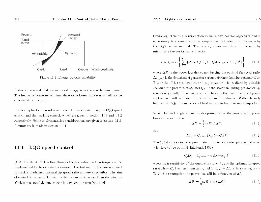
214 Chapter 11. Control Below Rated Power

r const.rω ω

increasedPower

Cut-in Rated Cut-out Wind speed [m/s]

Ratedpower

variable

Energy

Figure 11.2. Energy capture capability.

It should be noted that the increased energy is in the aerodynamic power.

The frequency converter will introduce some losses. However, it will not be

considered in this project.

In this chapter two control schemes will be investigated, i.e., the LQG speed

control and the tracking control, which are given in section 11.1 and 11.2

respectively. Some implementation considerations are given in section 11.3.

A summary is made in section 11.4.

11.1 LQG speed control

Control without pitch action through the generator reaction torque can be

implemented for below rated operation. The turbine in this case is caused

to track a prede�ned optimal tip speed ratio as close as possible. The aim

of control is to cause the wind turbine to extract energy from the wind as

e�ciently as possible, and meanwhile reduce the transient loads.

11.1 LQG speed control 215

Obviously, there is a contradiction between two control objectives and it

is necessary to choose a suitable compromise. A trade-o� can be made by

the LQG control method. The two objectives are taken into account by

minimizing the performance function

J(N; t) = E8<

:N�1X

j=0fQ1�Pr(t + j) + Q2(�Tg;ref (t+ j))2g

9=; (11.1)

where �Pr is the power loss due to not keeping the optimal tip speed ratio.

�Tg;ref is the deviation of generator torque reference from its optimal value.

The trade-o� between two control objectives can be realized by suitably

choosing the parameters Q1 and Q2. If the scalar weighting parameter Q2

is relatively small, the controller will emphasis on the maximization of power

capture and will use large torque variations to realize it. With relatively

high value of Q2, the reduction of load variations becomes more important.

When the pitch angle is �xed at its optimal value, the aerodynamic power

loss can be written as

�Pr =1

2��R2v3�Cp (11.2)

and

�Cp = Cp;max(�opt)� Cp(�) (11.3)

The Cp(�) curve can be approximated by a second order polynomial when

� is close to the optimal [Ekelund, 1994a]

Cp(�) = Cp;max � a0(� � �opt)2 (11.4)

where a0 is sensitivity of the quadratic curve, �opt is the optimal tip-speed

ratio where Cp has maximumvalue, and ���opt = �� is the tracking error.

With this assumption the power loss will be a function of ��

�Pr =1

2��R2v3a0(��)2 (11.5)

216

Chapter11.ControlBelowRatedPower

Thisimpliesthatthepowerlossisactuallydeterminedbythedeviationof

tip-speedratio��fromitsoptimalvalue.Theperformancefunction(11.1)

canthenbemodi�edby

J(N;t)=E

8 < :N�1 X j

=0

fQ1(��(t+j))2+Q2(�Tg;ref(t+j))2g9 = ;(11.6)

Sincethetipspeedratiocanbelinearizedatanoperatingpoint

��=

@�

@!r

? ? ? ? op�!r+

@�

@v

? ? ? ? op�v=Hx

(11.7)

where

H=[0

@�

@!r

00

@�

@v

]

x=[�� ��!r�!g�_v�v]T

whichleadstothecriterion

J(N;x(t))=E

8 < :N�1 X j

=0

fxT(t+j)Qxx(t+j)+Q2(�Tg;ref(t+j))2g9 = ; (1

1.8)

whereQx=HTQ1H.xisthestatevectorofthecompositestate-space

modelinpartialload.ThemodelhasbeengiveninChapter8.

TheLQcontrollawisimplementedbycombiningtheKalman�ltertoesti-

matethestatevector

u(t)=�L^x(t)

(11.9)

ThestepresponsesofgeneratortorqueTgandtipspeedratio�withdi�er-

entvaluesofweightingparameterQ2aregiveninFigure11.3andFigure

11.4respectively,wherethewindspeedchangesfrom9m/sto10m/sat1

11.1

LQG

speedcontrol

217

sec.The3P-e�ectisnotincludedinsimulationmodelforthestepresponses.

The�guresshowthatalargecontrolactionprovidesasmallsteady-state

erroroftipspeedratio.Theoptimalvalueoftipspeedratiois0.1357.

05

10

15

20

25

13

50

14

00

14

50

15

00

15

50

16

00

16

50

17

00

17

50

18

00

Tim

e [

s]

Tg [Nm]

1e

−9

3e

−9

6e

−9

1.5

e−

8

Figure11.3.ThestepresponseofgeneratortorqueTgwithdi�erentvalues

ofQ2whileQ1=1 0

51

01

52

02

50

.12

0.1

25

0.1

3

0.1

35

0.1

4

0.1

45

0.1

5

0.1

55

Tim

e [

s]

λ

1e

−9

3e

−9

6e

−9 1

.5e

−8

Figure11.4.Thestepresponseoftipspeedratio�withdi�erentvaluesof

Q2whileQ1=1

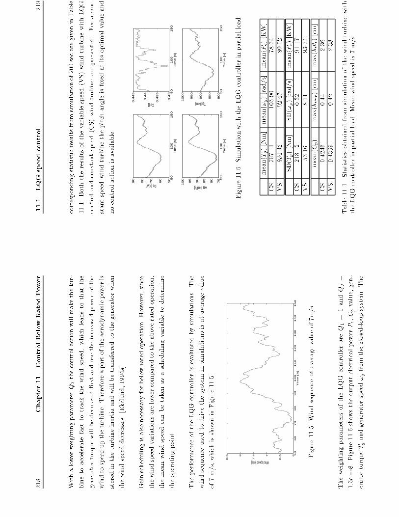
218

Chapter11.ControlBelowRatedPower

WithalowerweightingparameterQ2thecontrolactionwillmakethetur-

binetoacceleratefasttotrackthewindspeed,whichleadstothatthe

generatortorquewillbedecreased�rstandusetheincreasedpowerofthe

windtospeeduptheturbine.Thereforeapartoftheaerodynamicpoweris

storedintheturbineinertiaandwillbetransferredtothegeneratorwhen

thewindspeeddecreases[Ekelund,1994a].

Gainschedulingisalsonecessaryforbelowratedoperation.However,since

thewindspeedvariationsarelowercomparedtotheaboveratedoperation,

themeanwindspeedcanbetakenasaschedulingvariabletodetermine

theoperatingpoint.

TheperformanceoftheLQGcontrollerisevaluatedbysimulations.The

windsequenceusedtodrivethesysteminsimulationsisataveragevalue

of7m/s,whichisshowninFigure11.5.

50

60

70

80

90

10

01

10

12

01

30

14

01

50

6

6.57

7.58

8.5

Tim

e [S

]

Wind speed [m/s]

Figure11.5.Windsequenceataveragevalueof7m/s

TheweightingparametersoftheLQGcontrollerareQ1

=1andQ2

=

1:5e�8.Figure11.6showstheoutputelectricalpowerPe,Cpvalue,gen-

eratortorqueTgandgeneratorspeed!gfromtheclosed-loopsystem.The

11.1

LQG

speedcontrol

219

correspondingstatisticresultsfromsimulationof200secaregiveninTable

11.1.Boththeresultsofthevariablespeed(VS)windturbinewithLQG

controlandconstantspeed(CS)windturbinearepresented.Foracon-

stantspeedwindturbinethepitchangleis�xedatitsoptimalvalueand

nocontrolactionisavailable.

50

10

01

50

50

60

70

80

90

Tim

e [

s]

Pe [KW]

50

10

01

50

0.4

3

0.4

35

0.4

4

0.4

45

Tim

e [

s]

Cp []

50

10

01

50

75

80

85

90

95

10

0

Tim

e [

s]

wg [rad/s]

50

10

01

50

80

0

85

0

90

0

95

0

10

00

Tim

e [

s]

Tg [Nm]

Figure11.6.SimulationwiththeLQGcontrollerinpartialload.

mean(Tg)[Nm]

mean(!g)[rad/s]

mean(Pe)[KW]

CS

797.11

105.90

78.74

VS

934.32

92.47

80.92

SD(Tg)[Nm]

SD(!g)[rad/s]

mean(Pr)[KW]

CS

218.12

0.32

91.17

VS

53.16

8.11

93.74

mean(Cp)

max(ht!t)[cm]

max(ht�t)[cm]

CS

0.4246

0.44

2.36

VS

0.4399

0.42

2.38

Table11.1.Statisticsobtainedfromsimulationofthewindturbinewith

theLQGcontrollerinpartialload.Meanwindspeedis7m/s.

220

Chapter11.ControlBelowRatedPower

Thesimulationresultsindicatetheenergyincreasedbyvariablespeedoper-

ationisabout2.8%comparedtotheoutputoftheconstantspeedturbine.

However,evenwiththelittleincreaseofenergy,themeanvalueofCpis

ratherclosetoitsoptimalvalueof0:4440.Thereasonisthatthemeanvalue

ofCpfortheconstantspeedturbineatthisoperatingpointis0.4246,which

meansthereisnotsomuchextraenergythatcanbecapturedbyvariable

speedoperation.However,theenergyoutputofthewindturbinescanbe

increasedbyvariable-speedoperationdependingonwindvelocity.Forthe

WD34constantspeedwindturbine,whenthewindspeedisabout8.5m/s,

thetip-speedratioisratherclosetoitsoptimalvalue.Theincreasedenergy

byvariablespeedoperationnearthiswindspeedisverylittlecompared

totheconstantspeedwindturbine.However,thecapturedenergywillbe

increasedwhenthewindspeedleavesthisvalue.

mean(Tg)[Nm]

mean(!g)[rad/s]

mean(Pe)[KW]

CS

454.20

105.94

44.89

VS

695.16

78.74

51.28

SD(Tg)[Nm]

SD(!g)[rad/s]

mean(Pr)[KW]

CS

138.37

0.37

51.88

VS

48.98

5.81

59.36

mean(Cp)

max(ht!t)[cm]

max(ht�t)[cm]

CS

0.3784

0.30

1.89

VS

0.4409

0.28

1.70

Table11.2.Statisticsobtainedfromsimulationofthewindturbinewith

theLQGcontrollerinpartialload.Meanwindspeedis6m/s.

Anothersimulationiscarriedoutattheaveragewindspeedof6m/sandthe

sameweightingparametersoftheLQGcontrollerareused.Somekeyresults

fromsimulationsoftheconstantspeedandvariablespeedwindturbinewith

thesamewindsequencearegiveninTable11.2.Itcanbeeasilycalculated

11.2

Trackingcontrol

221

thatatthisoperatingpointtheincreasedenergyobtainedbyvariablespeed

operationisabout14.4%comparedtotheconstantspeedturbine.

Withvariablespeed,thetorquetransientsaresmoothedout.Theturbine

momentofinertiaactsasalow-pass�lter.However,withlargeinertia,the

angularvelocityofrotorcannotfollowthewindspeedvariationquickly,

whichwillleadtoatrackingerror.

Figure11.6showsthefastoscillationsingeneratortorquewhichiscaused

bythedisturbancesfrom

thetowershadow.Theoscillationsinducethe

mechanicalvibrationsontherotorshaft.

11.2

Trackingcontrol

Inthissectiontheoptimalcontrolproblemwillbetransformedtoatracking

problem,inwhichtheoptimaltipspeedratiowillbemaintainedbytracking

therotorspeedreference.

Inordertodeterminetheoptimaltipspeedratio�opt,thewindspeed

experiencedbytheturbineisrequiredtobeknown.However,sinceadirect

measurementofthee�ectivewindspeedisnotpossible,thewindspeed

mustbeestimatedfrom

measurementsmadeonthewindturbineitself.

Theoperatingpointisthendeterminedfromthisestimate.Theproblemof

windspeedestimationhasalreadybeendiscussedinChapter9.Hence,a

controllercanbeimplementedtotrackthe�optaccordingtotheestimated

windspeed.

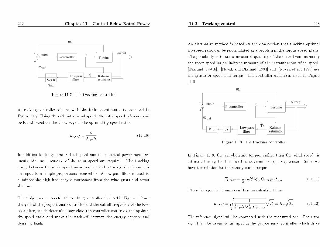
222 Chapter 11. Control Below Rated Power

estimatorKalman Low pass

filterλopt R.1

ωr,ref

P-controller

ωr

v

-

^

Turbine

Gain

error outputu

+

Figure 11.7. The tracking controller

A tracking controller scheme with the Kalman estimator is presented in

Figure 11.7. Using the estimated wind speed, the rotor speed reference can

be found based on the knowledge of the optimal tip speed ratio

!r;ref =

^v�optR

(11.10)

In addition to the generator shaft speed and the electrical power measure-

ments, the measurements of the rotor speed are required. The tracking

error, between the rotor speed measurement and rotor speed reference, is

an input to a simple proportional controller. A low-pass �lter is used to

eliminate the high frequency disturbances from the wind gusts and tower

shadow.

The design parameters for the tracking controller depicted in Figure 11.7 are

the gain of the proportional controller and the cut-o� frequency of the low-

pass �lter, which determine how close the controller can track the optimal

tip speed ratio and make the trade-o� between the energy capture and

dynamic loads.

11.2 Tracking control 223

An alternative method is based on the observation that tracking optimal

tip-speed ratio can be reformulated as a problem in the torque-speed plane.

The possibility is to use a measured quantity of the drive train, normally

the rotor speed as an indirect measure of the instantaneous wind speed.

[Ekelund, 1994b], [Novak and Ekelund, 1994] and [Novak et al., 1995] use

the generator speed and torque. The controller scheme is given in Figure

11.8.

ωK

r,ref

Turbineerror outputu

ωr

-

+

estimatorKalman Low pass

filterxT̂r

P-controller

ω

Figure 11.8. The tracking controller

In Figure 11.8, the aerodynamic torque, rather than the wind speed, is

estimated using the linearized aerodynamic torque expression. Since we

have the relation for the aerodynamic torque

Tr;max =1

2��R5�3optCp;max!

2r;opt (11.11)

The rotor speed reference can then be calculated from

!r;ref =s

1

12��R

5�3optCp;maxq^Tr = K!

q^Tr (11.12)

The reference signal will be compared with the measured one. The error

signal will be taken as an input to the proportional controller which drive

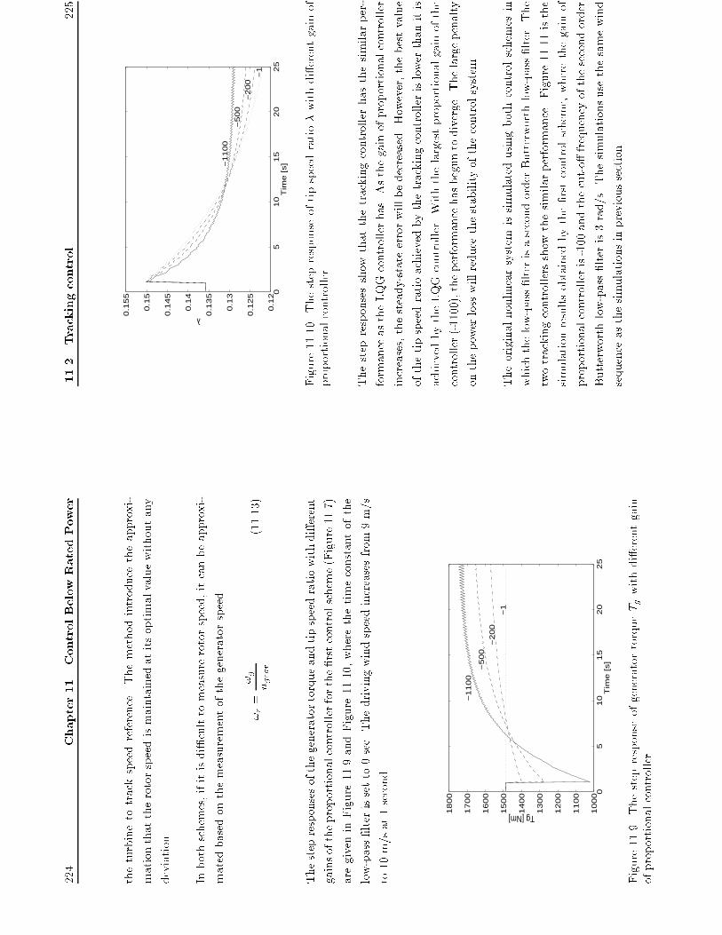
224

Chapter11.ControlBelowRatedPower

theturbinetotrackspeedreference.Themethodintroducetheapproxi-

mationthattherotorspeedismaintainedatitsoptimalvaluewithoutany

deviation.

Inbothschemes,ifitisdi�culttomeasurerotorspeed,itcanbeapproxi-

matedbasedonthemeasurementofthegeneratorspeed

!r=

!g

ngear

(11.13)

Thestepresponsesofthegeneratortorqueandtipspeedratiowithdi�erent

gainsoftheproportionalcontrollerforthe�rstcontrolscheme(Figure11.7)

aregiveninFigure11.9andFigure11.10,wherethetimeconstantofthe

low-pass�lterissetto0sec.Thedrivingwindspeedincreasesfrom9m/s

to10m/sat1second.

05

10

15

20

25

10

00

11

00

12

00

13

00

14

00

15

00

16

00

17

00

18

00

Tim

e [

s]

Tg [Nm]

−1

10

0

−5

00

−2

00

−1

Figure11.9.ThestepresponseofgeneratortorqueTgwithdi�erentgain

ofproportionalcontroller.

11.2

Trackingcontrol

225

05

10

15

20

25

0.1

2

0.1

25

0.1

3

0.1

35

0.1

4

0.1

45

0.1

5

0.1

55

Tim

e [

s]

λ

−1

10

0

−5

00

−2

00

−1

Figure11.10.Thestepresponseoftipspeedratio�withdi�erentgainof

proportionalcontroller.

Thestepresponsesshowthatthetrackingcontrollerhasthesimilarper-

formanceastheLQGcontrollerhas.Asthegainofproportionalcontroller

increases,thesteady-stateerrorwillbedecreased.However,thebestvalue

ofthetipspeedratioachievedbythetrackingcontrollerislowerthanitis

achievedbytheLQGcontroller.Withthelargestproportionalgainofthe

controller(-1100),theperformancehasbeguntodiverge.Thelargepenalty

onthepowerlosswillreducethestabilityofthecontrolsystem.

Theoriginalnonlinearsystem

issimulatedusingbothcontrolschemesin

whichthelow-pass�lterisasecondorderButterworthlow-pass�lter.The

twotrackingcontrollersshowthesimilarperformance.Figure11.11isthe

simulationresultsobtainedbythe�rstcontrolscheme,wherethegainof

proportionalcontrolleris-100andthecut-o�frequencyofthesecondorder

Butterworthlow-pass�lteris3rad/s.Thesimulationsusethesamewind

sequenceasthesimulationsinprevioussection.

226

Chapter11.ControlBelowRatedPower

50

10

01

50

55

60

65

70

75

80

85

Tim

e [

s]

Pe [KW]

50

10

01

50

0.4

2

0.4

25

0.4

3

0.4

35

0.4

4

0.4

45

Tim

e [

s]

Cp []

50

10

01

50

70

75

80

85

90

95

10

0

Tim

e [

s]

wg [rad/s]

50

10

01

50

84

0

86

0

88

0

90

0

92

0

94

0

Tim

e [

s]

Tg [Nm]

Figure11.11.Simulationwiththetrackingcontrollerinpartialload.

mean(Tg)[Nm]

mean(!g)[rad/s]

mean(Pe)[KW]

6m/s

672.20

80.57

50.58

7m/s

913.60

94.09

80.30

SD(Tg)[Nm]

SD(!g)[rad/s]

mean(Pr)[KW]

6m/s

23.61

7.75

59.03

7m/s

29.47

10.07

93.26

mean(Cp)

max(ht!t)[cm]

max(ht�t)[cm]

6m/s

0.4383

0.27

1.74

7m/s

0.4376

0.42

2.43

Table11.3.Statisticsobtainedfromsimulationofthewindturbinewith

thetrackingcontrollerinpartialload.Meanwindspeedis7m/s.

TheoutputpowerPe,generatorspeed!g,generatorreactiontorqueTgand

CpvalueobtainedfromthesimulationaregiveninFigure11.11.Somekey

parametersfromthesimulationaregiveninTable11.3whichshowsthatthe

trackingcontrollerhasthesimilarperformanceastheLQGcontroller.The

capturedpowerbyvariablespeedoperationisincreased2.3%ataverage

11.3

Implementationofcontrolsystem

227

windspeedof7m/sand13.8%ataveragewindspeedof6m/s,whichis

littlelessthanitisachievedbytheLQGcontrollerwithsimilarcontrol

action.However,thetrackingcontrollerseemsmoree�ectiveto�lterout

thefastvariationsinthegeneratortorquereferencebythelow-pass�lter

inthecontrolscheme,whichconsequentlyreducesthetransientloads.

11.3

Implementationofcontrolsystem

Sincethewindfrequentlyvariesfrom

belowtoaboveratedwindspeed

andviceversa,afundamentalrequirementforthewindturbineisasmooth

changesbetweenthetwocontrolschemes.Thisisthemostimportantimple-

mentationissueencounteredwhendevelopingcontrollersforwindturbines.

Forapitchregulatedconstantspeedwindturbine,belowacertainrated

windspeed,thegeneratedpowerislessthantheturbineratingandno

controlactionisrequired.Whenthewindspeedrisesaboverated,the

poweroutputisregulatedattheratedpowervaluebyadjustingthepitch

angleoftherotorblades.Henceitisnecessarytostartupandshutdown

thecontrollerautomaticallyasthewindspeed uctuates.Consequently,

thedesignofswitchingfrombelowratedtoaboveorviceversashouldbe

treatedwithsomecaretoavoidprolongtransientandtominimizetheloads

onthewindturbine.

Thetransientsassociatedwiththewindturbinecontrollerstart-upmaybe

attributedtosomeformofwindupwithinthecontrollerwhenoperatingbe-

lowrated.Thereforestart-upstrategyforreducingtheswitchingtransient

isconsideredwithinanti-windupcontext.

228

Chapter11.ControlBelowRatedPower

Whenthewindspeedfallsbelowrated,theactuatorwillbesaturated,the

controlfeedbackloopwillbebrokenandplantwillnolongerrespondto

thecontroller.However,thepureintegratorinthecontroller,introducedto

inducethecorrectsteadystateerrorbehaviour,continuestobedrivenby

thecontrolerroranditsoutputincreasesinmagnitudeorwindup.Conse-

quently,whenthecontrollerreturnstounsaturatedoperation,thetransient

willbeincreasedwhichcanleadtoalossofperformanceandinstability.

Acommonswitchingapproachtothecontrollerissimplytofreezecontroller

integralactionwhenbelowratedoperationisdetected,i.e.,whenthepitch

angledemandfallsbelowaspeci�edthresholdvalue,theaccumulationsum

intheintegralcalculationissuspended.Thisapproachisimplementedin

thisprojectandpreventsthepureintegratorinthecontrollerfromadopting

aninappropriatestateduringbelow-ratedoperation.However,ithasbeen

indicatedby

[LeithandLeithead,1997]thattheapproachisnotalways

e�ectiveinpreventinglargestart-uptransientsandthepoorperformance

willoccurwhenthereislow-frequencydynamicsinthecontroller.

[Leitheadetal.,1992]proposesanalternativestart-uptechniquewhereby

aminorfeedbackloopisintroducedwithinthecontrollerwhichswitchesin

topermitthecontrollertocontinueoperatingbelow-ratedwindspeed.The

minorfeedbackloopmimicstheactionofthephysicalwindturbinethrough

theinclusionofatransferfunctionwhichmodelsitsdynamics.

Thedynamicsofthewindturbinedrivetrainintroducealagbetween

changesinthewindspeedandcorrespondingchangesinpoweroutput,

i.e.,whenthewindspeedrisesaboverated,thereisalagbeforepower

outputrespondsandcontrolactionisresumed.[LeithandLeithead,1997]

11.3

Implementationofcontrolsystem

229

indicatesthattheswitchingperformancemightbeimprovedbyanticipat-

ingthetransientfrom

below-ratedtoaboveratedpowergenerationand

therebycompensatingforthedynamicsofthedrivetrain.Itwassuggested

toachievethepredictiveactionbyincludinga�lterwithsuitablephaselead

combinedwiththeminorfeedbackloop.

Forapitchregulatedvariablespeedwindturbine,switchingfrom

speed

controlviareferencetorqueinbelowratedwindspeedtospeedcontrolvia

pitchdemandandgeneratortorquecontrolviareferencetorqueinabove

windspeed,resultsincontrolerrorshavingdiscontinuous.Thevarious

controllertermsmustbeimplementedinsuchawaythatthesediscontinuous

donota�ecttheperformanceofthesystem.

[LeitheadandConnor,1994]givesaswitchingapproachtothecontroller

foravariablespeedpitchregulatedwindturbinebasedontheminorfeed-

backloop.Belowratedwindspeed,thegeneratortorquereferenceactson

theerrorinrotorspeedviathecontroller.Theminorfeedbackisoperational

andpitchdemandissettoaprede�nedoptimalvalue.Aboveratedwind

speed,theminoroffeedbackisinoperative,bothpitchangleandtorque

referenceactontheerrorinpowerviathecontroller.Switchingbetween

belowandaboveratedwindspeedisactivatedbypitchdemandchanging

sign.

Thetopicofswitchingbetweendi�erentcontrolschemesisnotdiscussedin

thisthesis.

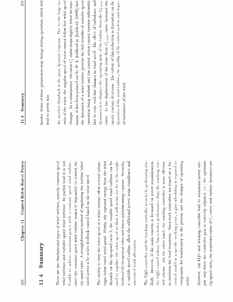
230

Chapter11.ControlBelowRatedPower

11.4

Summary

Therearetwofundamentaltypesofwindturbines,namely,constantspeed

windturbinesandvariablespeedwindturbines.Inpartialloaditisnot

feasibletoachievemaximumpowerwithaconstantspeedwindturbine,

sincetheconstantspeedwindturbinemakesitimpossibletocontrolthe

tipspeedratio.Astraightforwardmethodofregulatingtheturbinebelow

ratedpowerisbyactivefeedbackcontrolbasedontherotorspeed.

Theabilitytovarytherotorspeedofawindturbineo�ersseveraladvan-

tagesbelowratedwindspeed.Firstly,thecapturedenergyfromthewind

dependsonthetip-speedratio�,thevariablespeedwindturbinescanbe

usedtoregulatetherotorspeedsothat�willattain(orbeintheneigh-

borhoodof)itsoptimalvalueandhenceoptimizeenergycapture.Secondly,

avariablespeedturbineo�erstheadditionalpowertraincomplianceand

associatedloadsalleviation.

TheLQGcontrollerandthetrackingcontrollerseemtobeperformingsim-

ilarly.However,ifthemainconcernisfocussedonpowermaximization,

theLQGcontrolschemehasabetterperformancethanthetrackingcon-

trolscheme.Ontheotherhand,thetrackingcontrollerismoree�ective

tominimizetheloadtransients.Sincebothcontrollersarebasedonalin-

earizedmodelataspeci�cworkingpoint,againschedulingisrequiredto

compensatefornonlinearityintheprocessandthechangesofoperating

point.

However,theLQGandtrackingcontrollerleadtomaximumpowerout-

putonlywhenthecontrollergainiscorrectlyadjusted,i.e.,theoptimum

tip-speedratio,themaximumvalueofCp-curveandturbinedynamicsare

11.4

Summary

231

known.Someoftheseparametersmaychangeduringoperation,whichwill

leadtopowerloss.

Ananotherdrawbackisthepoordynamicresponse.Duetothelargein-

ertiaoftherotor,theangularspeedofrotorcannotfollowfastwindspeed

changes.Asaconsequence,themeanCp-valuedropsslightlybelowitsmax-

imum.IthasbeenpointedoutbyW.E.Leitheadin[Leithead,1989b]that

thedynamicsofawindturbinepreventthefullbene�tsofvariablespeed

operationbeingrealizedandthecontrolactioncannotoperatesu�ciently

fasttocopewithfastchangesinwindspeed.Thee�ectofturbulenceand

dynamicsistodisplacetheoperatingstateoftheturbinefromtheCp;max

curve.Asthedisplacementofthestatefrom

Cp:max

curveincreasesthe

energycapturedecreases.Theextentofthisreductionisdependentonthe

dynamicsofthewindturbine,thequalityofthecontrolsystemanddegree

ofturbulenceofthewind.

232

Chapter11.ControlBelowRatedPower

Chapter12

SummaryandConclusions

Theaimofthisprojectistoinvestigatethee�ectsofdi�erentcontrolsys-

temsforawindturbine.Theinvestigationsaredividedintobelowrated

operationandaboveratedoperation.Itisclearthatthewindturbinedy-

namicsandcontrolobjectiveschangelargelybetweendi�erentmodesof

operation.

AnonlinearwindturbinemodelbasedupontheexistingWD34windturbine

isdeveloped�rst.Allsigni�cantdynamicfeaturesencounteredonapracti-

calwindturbinehavebeenincludedinthemodelwithemphasisontheuse

ofsuchamodelintheevaluationandinvestigationofcontrolsystems.The

modelhasbeenvalidatedbyexperimentaldataobtainedfromtheWD34

windturbine.Thevalidationresultsshowagoodagreementbetweenex-

perimentaldataandsimulationoutput.Thenonlinearwindturbinemodel

isusedforsimulationpurpose.

233

234

Chapter12.SummaryandConclusions

Linearwindturbinemodelsarederivedfordesignofcontrolsystems.rated

operation,theactivepitchcontrolisimplementedforaconstantspeedwind

turbinetolimitthepowerandminimizetheloadtransients.However,a

pitchregulatevariablespeedwindturbinehastwocontrolvariables,namely

pitchangleandgeneratortorquereference,resultingamultivariablecontrol

problem.Thepitchdemandsvariedtoregulatethegeneratorspeedand

thereferencetorqueisvariedtoregulatethedrivetraintorques.Forbelow

ratedoperation,controlwithoutpitchactionthroughthegeneratorreaction

torqueisimplemented.Theturbineinthiscaseisasingleinputsingle

outputsystem.Inbothoperationmodesthedesignmodelsarelinearized

ataspeci�coperatingpoint.Thenonlinearityintheturbineleadstothat

themodelsdependontheoperatingpointsigni�cantly.

Theestimationofthewindspeedisdiscussedbeforetheinvestigationof

thecontrolsystems,sincesomecontrolmethodsmayneedtheknowledge

ofthewindspeed.Threedi�erentestimationmethodshavebeendeveloped

toestimatethewindspeed.Theinvestigationshowsthattheestimation

ofwindspeedisausefulmethodforcontroldesign.Caremustbetaken

whenimplementingtheestimationapproachessincethewindspeedcannot

beuniquelydeterminedinsomeoperatingarea.

Inpartialload,theaimofcontrolistoextractmaximumenergyfromwind

andmeanwhilereducethetransientloads.Sincetheenergyiscapturedby

theturbine,itisnaturaltooptimizetheperformancecriterionwithregard

totheaerodynamicpower.InordertoachievethemaximumCp,thetip

speedratioshouldbekeptatitsoptimalvalue.Thereforetheturbinespeed

mustfollowthechangesinwindspeed,whichrequireslargevariationsin

thecontrolsignalandconsequentlyincreasesthetransientloads.

235

Ifthemainconcernistominimizeshafttorquevariations,aturbinewith

alargeinertiaisprefered,sincetheaerodynamictorquevariationhasless

in uenceontheturbinespeedinthiscase.Ontheotherhanditisbetter

withsmallinertiawhenhighpowerproductionisprefered,becauseitde-

mandslesse�ecttochangetheturbinespeedinordertokeepthetipspeed

ratioconstant.

Infullload,thePIpitchcontrol,aswellastheLQGpitchcontrolandLQG

variablespeedpitchcontrolareinvestigated.Thesimulationresultsshow

thatthevariablespeedpitchcontrolprovidesthebestperformance.

Variablespeedoperationofhorizontalaxiswindturbineshasseveralpoten-

tialadvantages,ofwhichtwofrequentlymentionedonesaretheadditional

energycapturebelowratedwindspeedandtheadditionalpowertrain

complianceandassociatedloadalleviationaboveratedwindspeed.The

abilitytooperateatvaryingrotorspeede�ectivelyaddscompliancetothe

powertraindynamicsofthewindturbine.Anotherreasonforusingvari-

ablespeedoperationisthattherotorspeedcanbeadjustedtoreduce

noiselevelsandmakethewindturbinemoreenvironmentallyagreeable

[LeitheadandConnor,1994].

Thesebene�tsofusingvariablespeedturbinemustbeassessedagainstthe

disadvantages:thepowergenerationsystemismoreexpensiveduetothe

introductionofcomplexpowerconversionequipment.Anotherdisadvan-

tageisthatthee�ciencyandreliabilityofthevariablespeedturbineand

associatedcontrolsystemarereduced.

Theperformanceofvariablespeedwindturbinesisstronglydependenton

thethequalityofthecontrolsystemthroughitsabilitytoshapethedynamic

236

Chapter12.SummaryandConclusions

responseoftheturbinetowindspeedturbulence.Ithasbeenindicated

by[Leithead,1989b]thattheperformanceofvariablespeedwindturbine

istoanextentreducedbytheinteractionofthewindspeedturbulence

withthesystemdynamics.Belowratedwindspeedtheadditionalenergy

captureisinevitablyreducedfromthatwhichmightbeexpectedfromfully

exploitingthevariablespeedcapability.Aboveratedwindspeed,when

theregulationisgeneratorreactiontorquealone,theloadalleviationwhich

mightbeexpectedisagainreduced.Whenregulationisbypitchactionin

additiontogeneratortorque,improvedperformancecanbeexpected.

Themostimportantimplementationissueencounteredfordevelopingwind

turbinecontrollersissmoothchangebetweenthetwooperationmodes.The

mostsimpleswitchingapproachistofreezetheintegralactioninthecon-

trollerwhenbelowratedoperationisdetected.

Bibliography

[Andersenetal.,1980]Andersen,P.S.,Krabbe,U.,Lundsager,P.,and

Petersen,H.(1980).Basismaterialeforberegningafpropelvinm�lle.Tech-

nicalreport,Ris�NationalLaboratory.Ris�-M-2153.

[Bitmeadetal.,1990]Bitmead,R.R.,Gevers,M.,andWerts,V.(1990).

AdaptiveOptimalControl.Prentice-Hall.

[Bl�abjegandPetersen,1994]Bl�abjeg,F.and

Petersen,J.K.(1994).

Asynkronmotorenogdensstyringer.Teknisknytspecial1994.

[Bongersetal.,1990]Bongers,P.M.M.,Bierbooms,W.,Dijkstra,S.,and

vanHolten,T.(1990).Anintegrateddynamicmodelofa exiblewind

turbine.Technicalreport,DelftUniversityofTechnology,Holland.

[ConnorandLeithead,1994]Connor,B.andLeithead,W.E.(1994).Con-

trolstrategiesforvariablespeedstallregulatedwindturbines.In5th

EuropeanWindEnergyAssociationConferenceandExhibition,Greece.

[DennisandSchnabel,1983]Dennis,J.E.andSchnabel,R.B.(1983).

NumericalMethodsforUnconstrainedOptimizationandNonlinearEqua-

tions.Prentice-Hall,Inc.

237

238

BIBLIOGRAPHY

[Ekelund,1994a]Ekelund,T.(1994a).Controlofvariablespeedwindtur-

binesinabroadrangeofwindspeeds.Master'sthesis,ControlEngineer-

ingLaboratory,ChalmersUniversityofTechnology,G�oteborg,Sweden.

[Ekelund,1994b]Ekelund,T.(1994b).Speedcontrolofwindturbinesin

thestallregion.InTheProceedingsofthethirdIEEEConferenceon

ControlApplications,volumeVol.1,pagespp227{232,Glasgow.

[Ekelund,1997]Ekelund,T.(1997).ModelingandLinearQuadraticOpti-

malControlofWindTurbines.PhDthesis,ControlEngineeringLabora-

tory,ChalmersUniversityofTechnology,G�oteborg,Sweden.

[ErnstandLeonhard,1988]Ernst,J.andLeonhard,W.(1988).Optimiza-

tionoftheenergyoutputofvariablespeedwindturbine.InWindPower

85'SanFraniscoProceeding,volumeVol.1,pagesp.183{188.

[FlensborgandS�rensen,1995]Flensborg,J.andS�rensen,J.B.(1995).

Combinedvariablespeedandpitchcontrolforwindturbines.Master's

thesis,InstituteofElectronicSystem,AalborgUniversity.

[Franklinetal.,1990]Franklin,G.F.,Powell,J.D.,andPowell,M.L.

(1990).DigitalControlofDynamicSystems.Addison-WesleyPublishing

Company.

[Freris,1990]Freris,L.L.(1990).WindEnergyConversionSystems.Pren-

ticeHallInternational(UK)Ltd.

[Gelb,1974]Gelb,A.(1974).AppliedOptimalEstimation.Massachusetts

InstituteofTechnology.

[H�jstrup,1982]H�jstrup,J.(1982).Velocityspectraintheunstableplan-

etaryboundarylayer.JournaloftheAtmosphericSciences,Vol.39(No.

10).

BIBLIOGRAPHY

239

[Knudsen,1983]Knudsen,T.(1983).Reguleringafvindm�ller.Master's

thesis,IMSOR,DTH.Eksamensprojektnr.13/83.

[Knudsen,1989]Knudsen,T.(1989).Start/StopStrategierforVind-Diesel

Systemer.PhDthesis,IMSOR,DTH.Licentiatafhandlingnr.53.

[KostenkoandPiotrovsky,1969]Kostenko,M.andPiotrovsky,L.(1969).

ElectricalMachines,AlternatingCurrentMachines,volume2.MIRPub-

lishers,Moscow.

[KwakernaakandSiven,1972]Kwakernaak,H.andSiven,R.(1972).Lin-

earOptimalControlSystem.Wiley-interscience,JohnWiley&Sons,Inc.,

USA.

[Larsenetal.,1992]Larsen,S.E.,Courtney,M.,Hansen,F.A.,H�jstrup,

J.,andJensen,N.O.(1992).Turbulenceintensityandpowerspectra

70mabovethewatersurfaceofthegreatbelt.Technicalreport,Ris�

NationalLaboratory.Ris�-M-2898(EN).

[LeithandLeithead,1997]Leith,D.J.andLeithead,W.E.(1997).Im-

plementationofwindturbinecontrollers.Int.J.Control,Vol.66(No.

3).

[Leithead,1989a]Leithead,W.E.(1989a).Controlsystemsforwindtur-

bines.WindEngineering,Vol.13(No.6).

[Leithead,1989b]Leithead,W.E.(1989b).Variablespeedoperation-does

ithaveanyadvantages?WindEngineering,Vol.13(No.6).

[LeitheadandConnor,1994]Leithead,W.E.andConnor,B.(1994).Con-

trolofavariablespeedwindturbinewithinductiongenerator.InInter-

nationalConferenceonControl94,ConferencepublicationNo.389,IEE

1994.

240

BIBLIOGRAPHY

[Leitheadetal.,1990]Leithead,W.E.,Salle,S.A.D.L.,andReardon,

D.(1990).Windturbinecontrolobjectivesanddesign.InEuropean

CommunityWindEnergyConference,Madrid,Spain.

[Leitheadetal.,1991]Leithead,W.E.,Salle,S.A.D.L.,andReardon,D.

(1991).Poleandobjectivesofcontrolforwindturbines.IEEProceeding-

C,Vol.138(No.2).

[Leitheadetal.,1992]Leithead,W.E.,Salle,S.A.D.L.,andReardon,D.

(1992).Classicalcontrolofactiveregulationofconstantspeedhorizontal

axiswindturbines.Int.JournalofControl,Vol.55(No.4):845{876.

[NovakandEkelund,1994]Novak,P.andEkelund,T.(1994).Modeling,

identi�cationandcontrolofavariable-speedhawt.In5thEuropeanWind

EnergyAssociationConferenceandExhibition,Greece.

[Novaketal.,1995]Novak,P.,Ekelund,T.,Jovik,I.,andSchmidtbauer,

B.(1995).Modellingandcontrolofvariable-speedwindturbinedrive-

systemdynamics.IEEEControlSystems,Vol.15(no.4):p.28{38.

[�stergaard,1994]�stergaard,P.(1994).Pitchreguleringafenvindm�lle.

Master'sthesis,IMM,DTU.IMM-EKS-1994-27.

[Petersenetal.,1980]Petersen,E.L.,Troen,I.,andFrandsen,S.(1980).

Vindatlasfordanmark.Technicalreport,Ris�NationalLaboratory,Den-

mark.

[Poulsen,1985]Poulsen,N.K.(1985).RobustSelfTuningControllers.PhD

thesis,IMSOR,DTU,Denmark.

[Salleetal.,1990]Salle,S.A.D.L.,Reardon,D.,W.E.Leithead,andGrim-

ble,M.J.(1990).Reviewofwindturbinecontrol.Int.JournalofControl,

Vol.52:p.1295{111310.

BIBLIOGRAPHY

241

[Schmidtbauer,1994]Schmidtbauer,B.(1994).

Basdynamikochkom-

penseringsmetoderf�orvindturbin/generator.Technicalreport,Control

EngineeringLaboratory,G�oteborg,Sweden.ISSN0280-8927.

[Tsiolis,1994]Tsiolis,S.(1994).Asynkrongeneratorochfrekvensomriktare

f�ordriftavvindkraftverkmedvariabeltvarvtal.Technicalreport,School

ofElectricalandComputerEngineering,ChalmersUniversityofTech-

nology,G�oteborg,Sweden.

[Wilkieetal.,1990]Wilkie,J.,Leithead,W.E.,andAnderson,C.(1990).

Modellingofwindturbinesbysimplemodels.WindEngineering,Vol.

14(No.4).

242

BIBLIOGRAPHY

AppendixA

OptimizationBackground

Somebackgroundontheperformanceoptimizationwhichpreparestheway

foradaptiveextremum

controlhasbeengivenhere.Theunconstrained

optimizationproblemscanbesolvedbyagreatdealofnumericalmeth-

ods.Inthisappendixthemethodsconsideredtobeofparticularrele-

vancetotheextremumcontrolproblemswillbepresented,whichinclude

thehill-climbingmethod,gradientmethod,NewtonandGauss-Newton

method.Asacomplementofthesemethodsthelinesearchtechniqueis

introduced.Anintroductionoftheunconstrainedoptimizationhasbeen

givenby[Frandsenetal.95]and[DennisandSchnabel,1983].

243

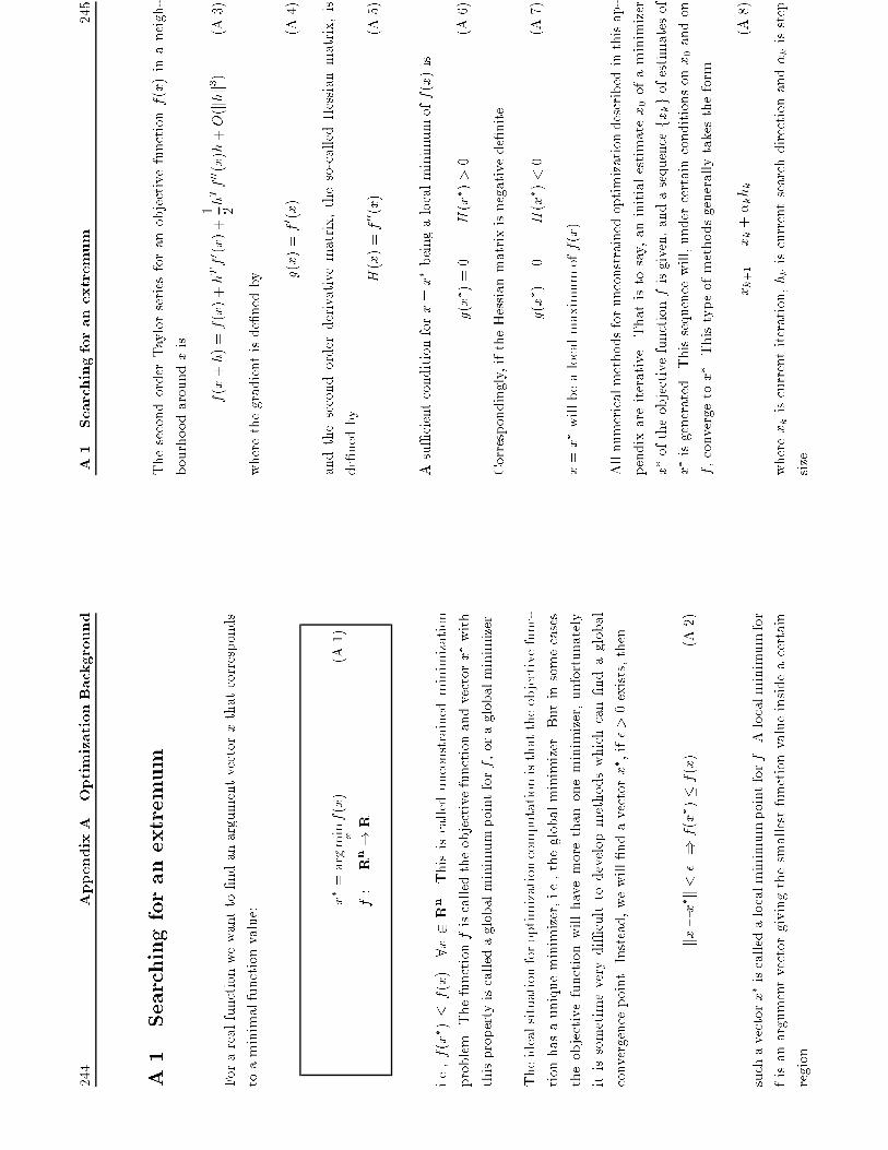
244

AppendixA.OptimizationBackground

A.1

Searchingforanextremum

Forarealfunctionwewantto�ndanargumentvectorxthatcorresponds

toaminimalfunctionvalue:

x�=argmin xf(x)

(A.1)

f:

Rn

!R

i.e.,f(x� )�f(x).8x2Rn.Thisiscalledunconstrainedminimization

problem.Thefunctionfiscalledtheobjectivefunctionandvectorx�with

thispropertyiscalledaglobalminimumpointforf,oraglobalminimizer.

Theidealsituationforoptimizationcomputationisthattheobjectivefunc-

tionhasauniqueminimizer,i.e.,theglobalminimizer.Butinsomecases

theobjectivefunctionwillhavemorethanoneminimizer,unfortunately

itissometimeverydi�culttodevelopmethodswhichcan�ndaglobal

convergencepoint.Instead,wewill�ndavectorx� ,if�>0exists,then

kx�x� k<�)f(x� )�f(x)

(A.2)

suchavectorx�iscalledalocalminimumpointforf.Alocalminimumfor

fisanargumentvectorgivingthesmallestfunctionvalueinsideacertain

region.

A.1

Searchingforanextremum

245

ThesecondorderTaylorseriesforanobjectivefunctionf(x)inaneigh-

bourhoodaroundxis

f(x+h)=f(x)+hTf0 (x)+

1 2hTf00 (x)h+O(khk3)

(A.3)

wherethegradientisde�nedby g

(x)=f0 (x)

(A.4)

andthesecondorderderivativematrix,theso-calledHessianmatrix,is

de�nedby

H(x)=f00 (x)

(A.5)

Asu�cientconditionforx=x�beingalocalminimumoff(x)is

g(x� )=0

H(x� )>0

(A.6)

Correspondingly,iftheHessianmatrixisnegativede�nite

g(x� )=0

H(x� )<0

(A.7)

x=x�willbealocalmaximumoff(x).

Allnumericalmethodsforunconstrainedoptimizationdescribedinthisap-

pendixareiterative.Thatistosay,aninitialestimatex0ofaminimizer

x�oftheobjectivefunctionfisgiven,andasequencefxkgofestimatesof

x�isgenerated.Thissequencewill,undercertainconditionsonx0andon

f,convergetox� .Thistypeofmethodsgenerallytakestheform

xk+1=xk+�khk

(A.8)

wherexkiscurrentiteration,hkiscurrentsearchdirectionand�kisstep

size.

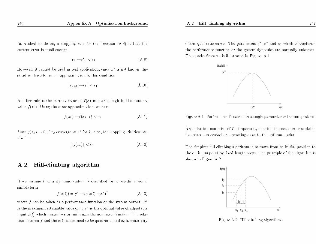
246 Appendix A. Optimization Background

As a ideal condition, a stopping rule for the iteration (A.8) is that the

current error is small enoughkxk � x�k < �1 (A.9)

However, it cannot be used in real application, since x� is not known. In-

stead we have to use an approximation to this condition

kxk+1 � xkk < �1 (A.10)

Another rule is the current value of f(x) is near enough to the minimal

value f(x�). Using the same approximation, we have

f(xk)� f(xk+1) < �2 (A.11)

Since g(xk)! 0, if xk converge to x� for k !1, the stopping criterion can

also be

kg(xk)k < �3 (A.12)

A.2 Hill-climbing algorithm

If we assume that a dynamic system is described by a one-dimensional

simple form

f(x(t)) = y� � a0(x(t)� x�)2 (A.13)

where f can be taken as a performance function or the system output. y�

is the maximum attainable value of f , x� is the optimal value of adjustable

input x(t) which maximizes or minimizes the nonlinear function. The rela-

tion between f and the x(t) is assumed to be quadratic, and a0 is sensitivity

A.2 Hill-climbing algorithm 247

of the quadratic curve. The parameters y�, x� and a0 which characterize

the performance function or the system dynamics are normally unknown.

The quadratic curve is illustrated in Figure A.1.

y

x* x(t)

f(x(t))

*

Figure A.1. Performance function for a single parameter extremum problem

A quadratic assumption of f is important, since it is in most cases acceptable

for extremum controllers operating close to the optimum point.

The simplest hill-climbing algorithm is to move from an initial position to

the optimum point by �xed length steps. The principle of the algorithm is

shown in Figure A.2.

x

f(x)

hh

x

3

f2

f

x x

f

1 2 3

1

Figure A.2. Hill-climbing algorithms

248

AppendixA.OptimizationBackground

wheref i=f(xi),i=1;2;3.Frompositionx(t)=x1,amovementx2=

x1+hismade,thevaluesf 1andf 2arecomparedbycalculatingperformance

function(A.13)whichisassumedknown.Iff 2islargethanf 1,x2=x1+h

istakenasthevalueofx(t+1),otherwisex2=x1�hisadopted.The

processiscontinueduntiltheextremumisreached.Thealgorithmcanbe

consideredasaspecialcaseofalgorithm(A.8),wherethestepsizeishand

thesearchdirectionis�1.

Sincetheinputsignalwillmovebackwardandforwardeithersideofthe

optimumeventually,x(t)willlieinaneighbourhoodoftheoptimalvaluex�

atlast.Ifwedecreasethesteplengthh,x(t)willbeclosertotheoptimal

value,buttheconvergencespeedwillbeslowdown.Ifweincreasethestep

lengthh,theoutputwillhaveasubstantialdistancebetweentheextremum,

althoughtheconvergencespeedisfast.

Thealgorithmcanmakestepsinthewrongdirectionbecauseofthepresence

ofthenoiseinthesystem.

A.3

Gradientmethod

Thegradientalgorithmorthesteepestdescentalgorithmallowsthehill-

climbingratetobeadjustedaccordingtothesizeofthegradient.Ateach

iterationthesearchdirectionismodi�edalongtheoppositedirectionofthe

gradient,i.e.,hk=�f0 (xk),whichiscalledthesteepestdecentdirection.

Inthiscasetheadjustmentrulefromxk+1toxkisgivenby

A.3

Gradientmethod

249

xk+1=xk��kg(xk)

(A.14)

whereg(xk)isthegradientde�nedin(A.4)and�k>0isagainparameter

whichcontrolstheconvergencerate.Thegradientmethodreliesona�rst

orderapproximationtotheobjectivefunctioninaneighbouringpointxk+1

toxk f

(xk+1)

=

f(xk)+(xk+1�xk)Tg(xk)+O(kxk+1�xkk2)

=

f(xk)��kg(xk)Tg(xk)+O(�2 k)

(A.15)

Ifthestepsize�k>0isadequatelysmall,the�rsttwotermsinthefunction

willdominateoverthelast,i.e.,thethirdtermisinsigni�cant.Itisthen

alwayspossibletoobtainareductionoftheobjectivefunction

f(xk+1)<f(xk)

Aconstantstepsizeisquiteoftenselected,whereasanumberofmethods

canbeappliedtoselectthestepsize�k,sincetheconvergenceraterelieson

it.AlinesearchmethodgiveninsectionA.6willingeneralgivethemost

rapidconvergence.

Theadvantageofthegradientalgorithmisthatthesizeoftheadjustment

ateachstepisdependentuponthesizeofthegradient.Theadjustmentstep

islargewhenthealgorithmisfarfromtheextremumandreduceswhenthe

extremumisclose.Butthealgorithmrequiresaknowledgeofthegradient

functionanditmightbesensitivetothenoise.Thegradientmethodhas

linearconvergence(convergenceoforder1),i.e.

kek+1k<c 1kekkwithc 1<1;xk

closetox�

(A.16)

250

AppendixA.OptimizationBackground

wheree k=xk�x� .Thegradientmethodismuchfasterthanthe�xed

steplengthmethods.

A.4

TheNewtonmethod

Whereasthegradientmethodreliesona�rstorderapproximationtothe

objectivefunction,thenewtonmethodisdeterminedasaminimizerofa

secondorderexpansionoftheobjectivefunctionatcurrentiterationxk

f(x)=f(xk)+(x�xk)Tf0 (xk)+

1 2(x�xk)Tf00 (xk)(x�xk)

(A.17)

Theideaisnowatiterationxktominimizetheobjectivefunctionf(x).If

theHessianH(xk)ispositivede�nite,f(x)willhaveauniqueminimizerat

apointwheref0 (x)=0,i.e.

g(xk)+H(xk)(x�xk)=0

whichleadsto

xk+1=xk�H(xk)�1g(xk)

(A.18)

Thisisalsoaspecialcaseofgeneralalgorithm(A.8),whenthestepsize

�k

=1andthesearchdirectionhk

=�H(xk)�1g(xk)whichiscalleda

Newtondirection.

AmaximumpointwillbefoundifH(xk)isnegativede�niteforallk.

IncaseH(xk)stayspositivede�niteforallkandifstartingpointissuf-

�cientclosetoaminimizer,themethodwillusuallyconvergeveryrapidly

towardstominimumpoint.Moreprecisely,theNewtonmethodconverges

A.4

TheNewtonmethod

251

quadraticallytowardx� ,i.e.,

kek+1k<c 2kekk2;xk

closetox�

(A.19)

ThedisadvantageoftheNewtonoptimizationalgorithmisthatitrequires

aknowledgeofboththegradientandsecondorderderivativeoftheper-

formancefunction.Thesemaybedi�cultto�ndeventhoughtheyare

knowntoexist.Butthemostseveredrawbackisthemethodlackofglobal

convergence.Whenxkisfarfromthesolution,f00 (xk)maynotbepositive

de�nite.Inthiscasetheiterationmayconvergetoasaddlepointoramax-

imizersincetheiterationisidenticaltotheoneusedforsolvingf0 (x)=0.

Anystationarypointoffisasolutiontothesystem.

The�rstmodi�cationistheNewtonmethodwithlinesearch,thereforethe

iterationismodi�edby x

k+1=xk��kH(xk)�1g(xk)

(A.20)

wherethestepsize�kisdeterminedbylinesearchalgorithmwhichwillbe

giveninsectionA.6.

Anotherideaistotaketheadvantageofthesafeconvergenceproperties

ofthegradientmethodwhenevertheNewtonmethodgetsintotrouble.

Thegradientmethodisselected,whenxkisfarfromtheconvergencepoint

wheretheHessianmaynotbepositivede�nite.TheNewtonmethodisse-

lected,whenxkisclosetotheconvergencepointwherethegradientmethod

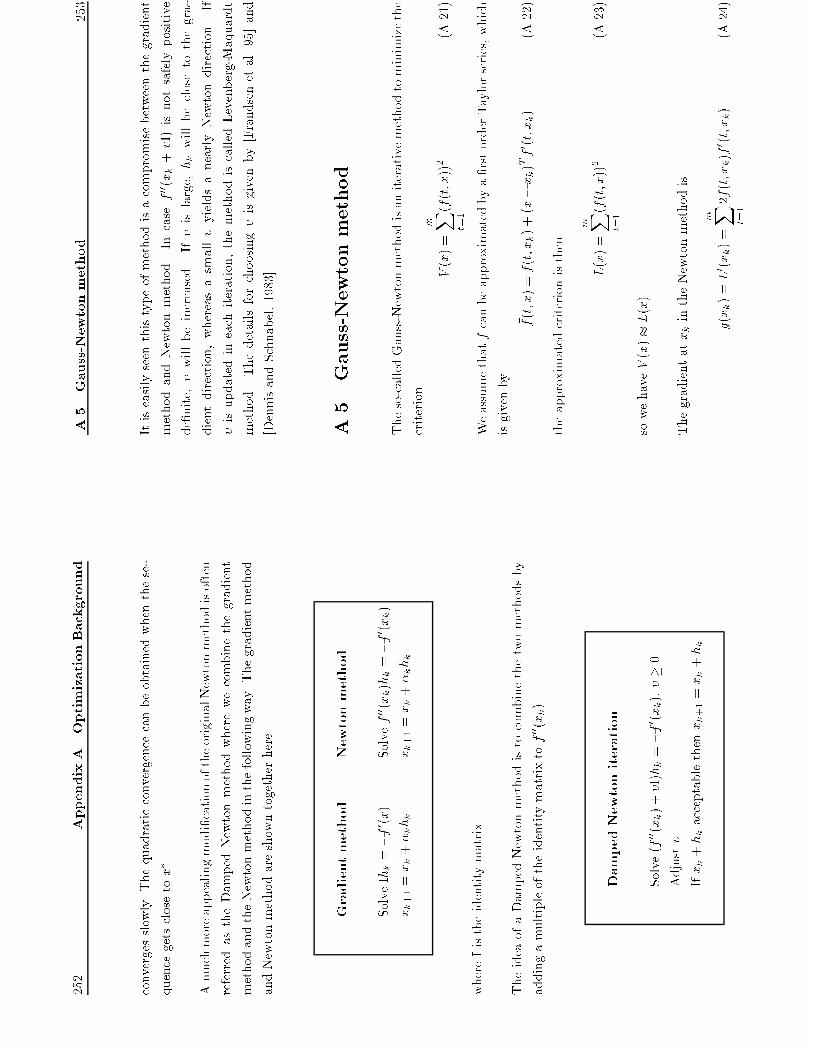
252

AppendixA.OptimizationBackground

convergesslowly.Thequadraticconvergencecanbeobtainedwhenthese-

quencegetsclosetox� .

Amuchmoreappealingmodi�cationoftheoriginalNewtonmethodisoften

referredastheDampedNewtonmethodwherewecombinethegradient

methodandtheNewtonmethodinthefollowingway.Thegradientmethod

andNewtonmethodareshowntogetherhere

Gradientmethod

Newtonmethod

SolveIhk=�f0 (x)

Solvef00 (xk)hk=�f0 (xk)

xk+1=xk+�khk

xk+1=xk+�khk

whereIistheidentitymatrix.

TheideaofaDampedNewtonmethodistocombinethetwomethodsby

addingamultipleoftheidentitymatrixtof00 (xk).

DampedNewtoniteration

Solve(f00 (xk)+�I)hk=�f0 (xk),��0

Adjust�

Ifxk+hkacceptablethenxk+1=xk+hk.

A.5

Gauss-Newtonmethod

253

Itiseasilyseenthistypeofmethodisacompromisebetweenthegradient

methodandNewtonmethod.Incasef00 (xk+�I)isnotsafelypositive

de�nite,�willbeincreased.If�islarge,hk

willbeclosetothegra-

dientdirection,whereasasmall�yieldsanearlyNewtondirection.If

�isupdatedineachiteration,themethodiscalledLevenberg-Maquardt

method.Thedetailsforchoosing�isgivenby[Frandsenetal.95]and

[DennisandSchnabel,1983].

A.5

Gauss-Newtonmethod

Theso-calledGauss-Newtonmethodisaniterativemethodtominimizethe

criterion

V(x)=

m X t=1

(f(t;x))2

(A.21)

Weassumethatfcanbeapproximatedbya�rstorderTaylorseries,which

isgivenby

� f(t;x)=f(t;xk)+(x�xk)Tf0 (t;xk)

(A.22)

theapproximatedcriterionisthen

L(x)=

m X t=1

(� f(t;x))2

(A.23)

sowehaveV(x)�L(x)

ThegradientatxkintheNewtonmethodis

g(xk)=L0 (xk)=

m X t=1

2� f(t;xk)f0 (t;xk)

(A.24)

254

AppendixA.OptimizationBackground

andHessianis

R(xk)=

m X t=1

2f0 (t;xk)f0 (t;xk)

(A.25)

R(xk)iscalledtheGauss-NewtonHessiananditisobviouslypositivesemidef-

inite.TheGauss-NewtoniterationisderivedasaminimizerofL(x)

xk+1=xk��kR(xk)�

1g(xk)

(A.26)

Inpracticetheiterationshouldbecomplementedwithaline-searchfor

determiningthestepsize�k.ItisclearthattheNewtonandGauss-Newton

methodsareidentical,whenthesecondorderderivativecanbeneglected.

TheGauss-Newtonhastheattractivepropertythatitrequiresonlya�rst

orderderivative.Thelocalconvergenceofthemethodisingeneralonly

linear(�rstorder),whichistheoreticallyslowerthantheNewtonmethod.

Butexperiencesshowthatitisoftenfasterinpractice.Inparticularwhen

itisusedfarfromtheminimum.AnotherproblemintheGauss-Newton

methodisthattheR(xk)maybesingularorill-conditioning.Itcanbe

solvingbyaddingasmalldiagonalmatrixtotheHessian.

A.6

Linesearchtechnique

InsomecasesthegradientmethodorNewtonmethodwillbecomplemented

byalinesearch,becausethealgorithm

isderivedfrom

a�rstorderor

secondorderapproximationtotheobjectivefunction.Theapproximation

A.6

Linesearchtechnique

255

willusuallybevalidonlyinacertainneighborhoodaroundthecurrent

iteration.Thefullstep�k=1mightbringthenewiterationtoalocation

thatisfarfromthepointpredictedbytheapproximation.

Theideaoflinesearchmethodsis:whenagradientdirectionoraNewton

directionhasbeendetermined,wehavetodecidehowlongthestepinthis

directionshouldbe.Afrequentlyusedmethodfordeterminingstepsize�k

istoestimatealocalminimizeroff(xk+�hk)regardedasafunctionof�

f(xk+�khk)=min�>0f(xk+�hk)

(A.27)

Introducethenotation

'(�)=f(xk+�hk)

(A.28)

thenonemethodofdetermining�kistoestimatealocalminimizerof',

sothat�ksatis�es

'0 (�)=0

(A.29)

Ingeneral,(A.29)isanonlinearequationanddi�culttosolveanalyti-

cally.Thereforesomenumericalmethodsforestimatingavalueof�which

satis�es(A.27)mustbeused.Mostlinesearchesareiterativeprocedures

whichareterminatedwhenthecurrentestimateof�ksatis�esagivenset

ofconvergencecriteria.Linesearchesarethereforeusuallynotexact.

Themethodswhichareusedfrequentlyforestimating�karebaseduponthe

ideaofapproximating'de�nedby(A.28)byapolynomialin�ofdegreetwo

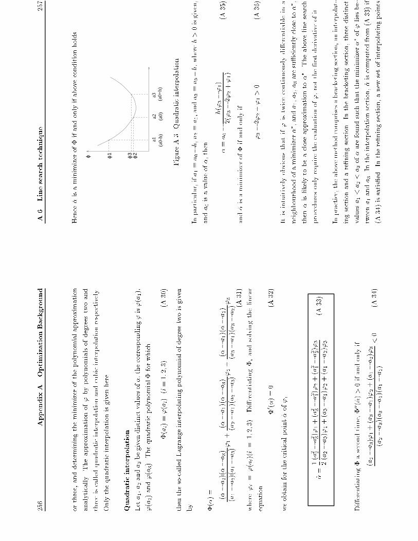
256

AppendixA.OptimizationBackground

orthree,anddeterminingtheminimizerofthepolynomialapproximation

analytically.Theapproximationof'bypolynomialsofdegreestwoand

threeiscalledquadraticinterpolationandcubicinterpolationrespectively.

Onlythequadraticinterpolationisgivenhere.

Quadraticinterpolation

Leta1,a2anda3begivendistinctvaluesof�,thecorresponding'is'(a1),

'(a2)and'(a3).Thequadraticpolynomial�forwhich

�(ai)='(ai)(i=1;2;3)

(A.30)

thentheso-calledLagrangeinterpolatingpolynomialofdegreetwoisgiven

by

�(�)=

(��a2)(��a3)

(a1�a2)(a1�a3)'

1+

(��a1)(��a3)

(a2�a1)(a2�a3)'

2+

(��a1)(��a2)

(a3�a1)(a3�a2)'

3

(A.31)

where'i=

'(ai)(i=

1;2;3).Di�erentiating�,andsolvingthelinear

equation

�0 (�)=0

(A.32)

weobtainforthecriticalpoint^�of',

^�=

1 2(a2 2�a2 3)'1+(a2 3�a2 1)'2+(a2 1�a2 2)'3

(a2�a3)'1+(a3�a1)'2+(a1�a2)'3

(A.33)

Di�erentiating�asecondtime,�00 (^�)>0ifandonlyif

(a2�a3)'1+(a3�a1)'2+(a1�a2)'3

(a2�a3)(a3�a1)(a1�a2)

<0

(A.34)

A.6

Linesearchtechnique

257

Hence^�isaminimizerof�ifandonlyifaboveconditionholds.

(a0+

h)

ϕ ϕ1

a1a2

a3

ϕ2ϕ3

(a0)

(a0-

h)FigureA.3.Quadraticinterpolation

Inparticular,ifa1=a0�h,a2=a0,anda3=a0+h,whereh>0isgiven,

anda0isavalueof�,then

^�=a0�

h('3�'1)

2('3�2'2+'1)

(A.35)

and^�isaminimizerof�ifandonlyif

'3�2'2+'1>0

(A.36)

Itisintuitivelyobviousthatif'istwicecontinuouslydi�erentiableina

neighbourhoodofaminimizer�� ,anda1,a2,a3aresu�cientlycloseto�� ,

then^�islikelytobeacloseapproximationto�� .Theabovelinesearch

proceduresonlyrequiretheevaluationof',notthe�rstderivativeofit.

Inpractice,theabovemethodcomprisesabracketingsection,aninterpolat-

ingsectionandare�ningsection.Inthebracketingsection,threedistinct

valuesa1<a2<a3of�arefoundsuchthattheminimizer��of'liesbe-

tweena1anda3.Intheinterpolationsection,^�iscomputedfrom(A.33)if

(A.34)issatis�ed.Inthere�ningsection,anewsetofinterpolatingpoints

258

AppendixA.OptimizationBackground

isselectedfroma1,a2,a3and^�,if^�isnotasu�cientlygoodestimateof

�� ,andinterpolationsectionisre-entered.Theinterpolatingandre�ning

sectionareusedrepeatedlyuntil^�isregardedasasu�cientlygoodesti-

mateof�� .Detailsofthebracketingsectionandthere�ningsectionare

givenby[Wolfe78].

A.7

Summary

Thisappendixgivesanintroductionofunconstrainedoptimizationtech-

niquesasabackgroundknowledgetotheextremumcontrolproblem.In

thechapterthehill-climbingmethod,gradientmethod,NewtonandGauss-

Newtonmethodareintroduced.ThegradientmethodorNewtontype

methodscanbeincorporatedwithlinesearch.

Thegradientmethodhasalinear�nalconvergence,whichisslowerthanthe

Newtonmethodthathasasecondorderconvergence.Thesizeofadjustment

inthegradientmethodateachiterationisdependentuponthesizeofthe

gradient.Theadjustmentislargeandthealgorithmconvergesfastwhen

xk

isfarfrom

theconvergencepoint.Theadjustmentissmallandthe

algorithmconvergesslowlywhenxkisclosetotheconvergencepoint.

TheNewtonmethodissimpleandclearandthuseasytoimplement,the

methodconvergesquadraticallyfromgoodstartingguessiff00 (x� )isposi-

tivede�nite.ButtheNewtonmethodlacksofglobalconvergenceformany

problems.Itrequiressecondorderderivativeoff,besidesf00 (xk)maynot

bepositive.TheNewtonmethodcanbemodi�edbycombiningtheline

searchwherethestepsize�kwillbedeterminedateachstep.Foraspecial

A.7

Summary

259

criterion,theGauss-NewtonmethodcanguaranteetheHessianispositive

semide�nite.

ThegradientmethodandNewtonmethodcanbecombinedandusedfor

di�erentsituations.Thegradientmethodisselected,whenxkisfarfrom

thex� .TheNewtonmethodistaken,whenxk

isclosetothex� .The

combinedalgorithmtaketheadvantageofthesafeconvergenceproperty

ofthegradientmethodandquadraticconvergencepropertyoftheNewton

method.

Byimplementingthelinesearchalgorithm,thestepsize�k

usuallypro-

ducesasatisfactorydecreaseinthevalueoffateachiterationwhena

searchdirectionisdetermined.However,thelinesearchiscomputationally

expensive.

260

AppendixA.OptimizationBackground

AppendixB

ConvergenceAnalysisfor

RecursiveAlgorithms

Inthissectionageneralapproachtotheanalysisoftheasymptoticbe-

haviourofrecursivealgorithmsisdescribed.

Ine�ect,theconvergence

analysisisreducedtostabilityanalysisofadeterministicOrdinaryDif-

ferentialEquation(ODE).Theapproachusedforanalysisisdevelopedby

Ljung,see[Ljung77]and[WellsteadandZarrop91].Herewejustgivea

briefsummarization.

Convergencepropertiescanbestatedas

1.Thesystemisstable.

2.Themodelparameterestimatesconverge.

3.Theestimatesconvergetocorrectvalues.

261

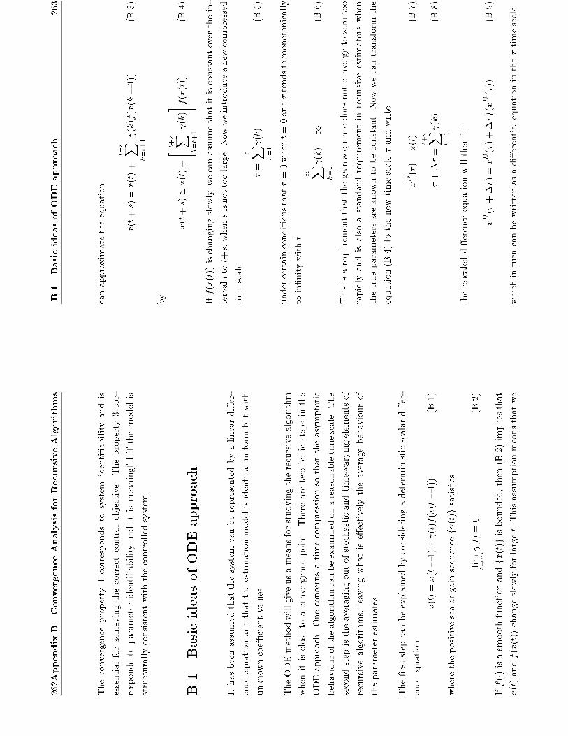
262AppendixB.ConvergenceAnalysisforRecursiveAlgorithms

Theconvergenceproperty1correspondstosystem

identi�abilityandis

essentialforachievingthecorrectcontrolobjective.Theproperty3cor-

respondstoparameteridenti�abilityanditismeaningfulifthemodelis

structurallyconsistentwiththecontrolledsystem.

B.1

BasicideasofODEapproach

Ithasbeenassumedthatthesystemcanberepresentedbyalineardi�er-

enceequationandthattheestimationmodelisidenticalinformbutwith

unknowncoe�cientvalues.

TheODEmethodwillgiveusameansforstudyingtherecursivealgorithm

whenitisclosetoaconvergencepoint.Therearetwobasicstepsinthe

ODEapproach.Oneconcernsatimecompressionsothattheasymptotic

behaviourofthealgorithmcanbeexaminedonareasonabletimescale.The

secondstepistheaveragingoutofstochasticandtime-varyingelementsof

recursivealgorithms,leavingwhatise�ectivelytheaveragebehaviourof

theparameterestimates.

The�rststepcanbeexplainedbyconsideringadeterministicscalardi�er-

enceequation

x(t)=x(t�1)+ (t)f(x(t�1))

(B.1)

wherethepositivescalargainsequencef (t)gsatis�es

limt!1 (t)=0

(B.2)

Iff(�)isasmoothfunctionandfx(t)gisbounded,then(B.2)impliesthat

x(t)andf(x(t))changeslowlyforlarget.Thisassumptionmeansthatwe

B.1

BasicideasofODEapproach

263

canapproximatetheequation

x(t+s)=x(t)+

t+s X

k=t+1

(k)f(x(k�1))

(B.3)

by

x(t+s)'x(t)+

" t+s X

k=t+1

(k)# f(x(t))

(B.4)

Iff(x(t))ischangingslowly,wecanassumethatitisconstantoverthein-

tervalttot+s,whensisnottoolarge.Nowweintroduceanewcompressed

timescale

�=

t X k=1

(k)

(B.5)

undercertainconditionsthat�=0whent=0and�tendstomonotonically

toin�nitywitht

1 X k=1

(k)=1

(B.6)

Thisisarequirementthatthegainsequencedoesnotconvergetozerotoo

rapidlyandisalsoastandardrequirementinrecursiveestimatorswhen

thetrueparametersareknowntobeconstant.Nowwecantransformthe

equation(B.4)tothenewtimescale�andwrite

xD(�)=x(t)

(B.7)

�+��=

t+s X k

=1

(k)

(B.8)

therescaleddi�erenceequationwillthenbe

xD(�+��)=xD(�)+��f(xD(�))

(B.9)

whichinturncanbewrittenasadi�erentialequationinthe�timescale

264AppendixB.ConvergenceAnalysisforRecursiveAlgorithms

d d�

xD(�)=f(xD(�))

(B.10)

inthelimitass(��)goestozero.ThisisanODE.Theasymptotic

behaviouroforiginaldi�erenceequation(B.1)isclosetothetrajectoriesof

theODE(B.10).TheODEismainlyatoolforexamininglocalconvergence.

Itispossibletogeneralizethesimplescalarrecursionbymakingthefunction

f(x(t))inequation(B.1)dependentuponafurthervariable'(t).The

equation(B.1)canbereplacedby

x(t)=x(t�1)+ (t)Q(t;x(t�1);'(t))

(B.11)

Weshallrefertox(�)astheestimatesandtheycouldbethecurrentesti-

matesofsomeunknownparametervector.Thevector'(t)isanobservation

obtainedattimet,andthesearetheobjectsthatcausex(t�1)tobeup-

datedtotakenewinformationintoaccount.Theobservationsareingeneral

functionsofthepreviousestimatesx(�)andofasequenceofrandomvectors

e(�).Thismeansthattheobservationisarandomvariable,whichmaybe

a�ectedbypreviousestimates.Thefollowingstructureforthegeneration

of'(t)willbeused

'(t)=A(x(t�1))'(t�1)+B(x(t�1))e(t)

(B.12)

Let D

s=fxjA(x)hasalleigenvaluesstrictlyinsidetheunitcircleg(B.13)

andforeachx2Ds,wede�neaasymptoticstationaryprocess

�'(t;x)=A(x)�'(t�1;x)+B(x)e(t)

�'(0;x)=0

(B.14)

B.1

BasicideasofODEapproach

265

andfurthermorewede�nethefunction

f(x)=

limt!1EQ(t;x;�'(t;x))

(B.15)

Theexpectationoperationsmoothesthein uenceofrandomcomponents

whichmaydisguisetheconvergencecharacteristicsoftherecursivealgo-

rithm.Theequation(B.11)canthenbeagainwrittenasordinarydi�eren-

tialequation(B.10).

Iff(x(t))iscontinuouslydi�erentiablewithrespecttoxinaneighborhood

ofastationarypointx�andderivativesconvergeuniformlyinthisneigh-

borhoodasttendstoin�nity.Then

f(x� )=0

(B.16)

and

H(x� )=

d dx

f(x)� � � � x=x

�

hasalleigenvaluesintheLHP

(B.17)

ThematrixH(x� )de�nesthelineardi�erentialequationobtainedfrom

(B.10)bylinearizationaroundx� .Theaboveequationsstatethatthe

algorithm(B.1)or(B.11)canconvergeonlytostablestationarypointsof

thedi�erentialequation(B.10).

Equations(B.16)and(B.17)arenecessaryconditionsforthelocalcon-

vergenceofrecursion(B.1)tox� .Theseconditionsarenotsu�cientand

thereforedonotguaranteeconvergence.Theequations(B.16)and(B.17)

arenormallyusedtocheckthepossiblelocalconvergencepoints.

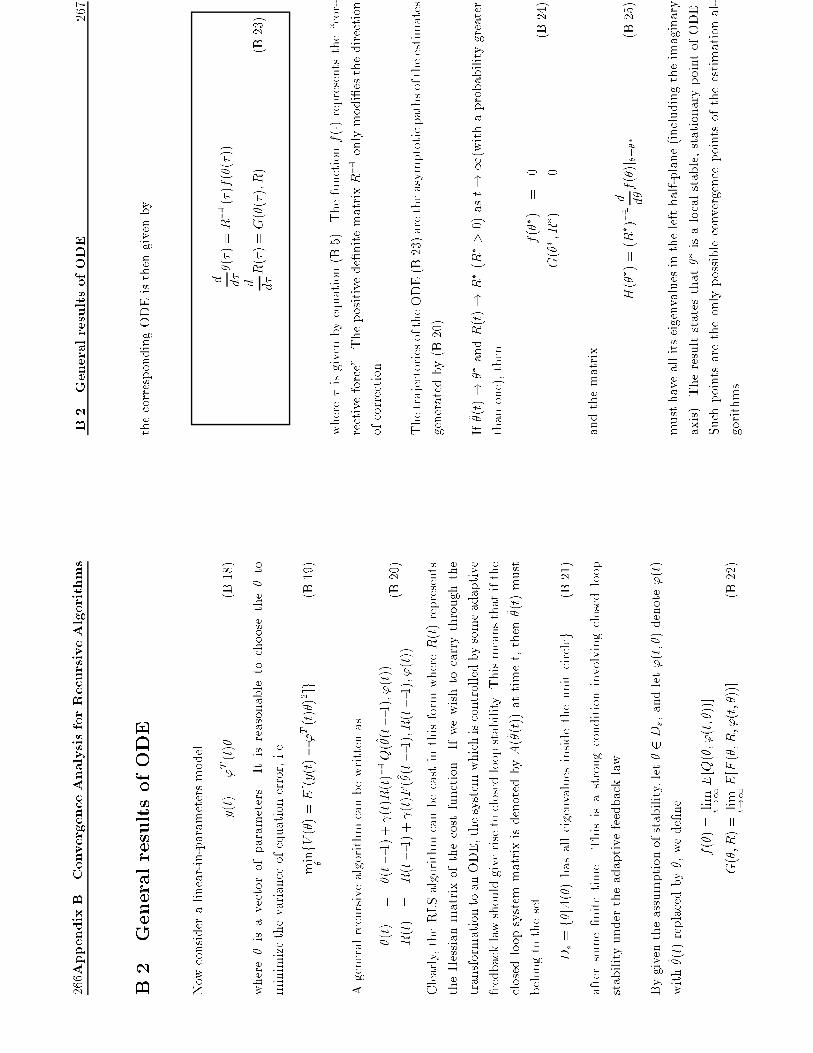
266AppendixB.ConvergenceAnalysisforRecursiveAlgorithms

B.2

GeneralresultsofODE

Nowconsideralinear-in-parametersmodel

y(t)='T(t)�

(B.18)

where�isavectorofparameters.Itisreasonabletochoosethe�to

minimizethevarianceofequationerror,i.e.

min �fV(�)=E[(y(t)�'T(t)�)2]g

(B.19)

Ageneralrecursivealgorithmcanbewrittenas

^ �(t)

=

^ �(t�1)+ (t)R(t)�1Q(^ �(t�1);'(t))

R(t)

=

R(t�1)+ (t)F(^ �(t�1);R(t�1);'(t))

(B.20)

Clearly,theRLSalgorithmcanbecastinthisformwhereR(t)represents

theHessianmatrixofthecostfunction.Ifwewishtocarrythroughthe

transformationtoanODE,thesystemwhichiscontrolledbysomeadaptive

feedbacklawshouldgiverisetoclosedloopstability.Thismeansthatifthe

closedloopsystemmatrixisdenotedbyA(^ �(t))attimet,then^ �(t)must

belongtotheset

Ds=f�jA(�)hasalleigenvaluesinsidetheunitcircleg

(B.21)

aftersome�nitetime.Thisisastrongconditioninvolvingclosedloop

stabilityundertheadaptivefeedbacklaw.

Bygiventheassumptionofstability,let�2Ds,andlet�'(t;�)denote'(t)

with^ �(t)replacedby�,wede�ne

f(�)=

limt!1E[Q(�;�'(t;�))]

G(�;R)=

limt!1E[F(�;R;�'(t;�))]

(B.22)

B.2

GeneralresultsofODE

267

thecorrespondingODEisthengivenby

d d�

�(�)=R�1(�)f(�(�))

d d�

R(�)=G(�(�);R)

(B.23)

where�isgivenbyequation(B.5).Thefunctionf(�)representsthe\cor-

rectiveforce".Thepositivede�nitematrixR�1onlymodi�esthedirection

ofcorrection.

ThetrajectoriesoftheODE(B.23)aretheasymptoticpathsoftheestimates

generatedby(B.20).

If^ �(t)!��andR(t)!R�(R�>0)ast!1(withaprobabilitygreater

thanone),then

f(�� )=

0

G(�� ;R� )=

0

(B.24)

andthematrix

H(�� )=(R� )�1d d

�f(�)j �=��

(B.25)

musthaveallitseigenvaluesinthelefthalf-plane(includingtheimaginary

axis).Theresultstatesthat��isalocalstable,stationarypointofODE.

Suchpointsaretheonlypossibleconvergencepointsoftheestimational-

gorithms.

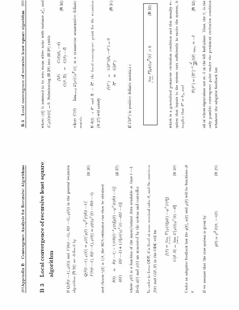
268AppendixB.ConvergenceAnalysisforRecursiveAlgorithms

B.3

Localconvergenceofrecursiveleastsquare

algorithm

IfQ(^ �(t�1);'(t))andF(^ �(t�1);R(t�1);'(t))inthegeneralrecursive

algorithm(B.20)arede�nedby

Q(^ �(t�1);'(t))='(t)[y(t)�'T(t)^ �(t�1)]

F(^ �(t�1);R(t�1);'(t))='(t)'T(t)�R(t�1)

(B.26)

andchoose (t)=1=t,theRLSestimatorcanthenbeobtained

^ �(t)

=

^ �(t�1)+1=tR(t)�1'(t)[y(t)�'T(t)^ �(t�1)]

R(t)

=

R(t�1)+1=t['(t)'T(t)�R(t�1)]

(B.27)

where'(t)isafunctionoftheinput/outputdataavailableattimet�1.

Bothy(t)and'(t)aregeneratedbythesystemandcontroller.

InordertoformODE,^ �is�xedatsomenominalvalue�,andthematrices

f(�)andG(�;R)intheODEwillbe

f(�)=

limt!1Ef'(t)[y(t)�'T(t)�]g

G(�;R)=

limt!1Ef'(t)'T(t)�R]

(B.28)

Underanadaptivefeedbacklawthey(t),u(t)and'(t)willbefunctionsof

�. Ifweassumethatthetruesystemisgivenby

y(t)='T(t)�0+e(t)

(B.29)

B.3

Localconvergenceofrecursiveleastsquarealgorithm

269

wheree(t)isassumedtobezeromeanwhitenoisewithvariance�2 e,and

E['(t)e(t)]=0.Substituting(B.29)into(B.28)yields

f(�)

=

G(�)(� 0��)

G(�;R)

=

G(�)�R

(B.30)

whereG(�)=

limt!1E['(t)'T(t)]isasymmetricnonnegativede�nite

matrix.

If^ �(t)!��andR!R� ,thelocalconvergencepointfortherecursion

(B.27)willsatisfy

f(�� )=

G(�� )(�0���)=0

R�=

G(�� )

(B.31)

IfG(�� )ispositivede�nitematrix,i.e.

limt!1E['(t)'T(t)]>0

(B.32)

whichisageneralizedpersistentexcitationconditionandthisusuallyre-

quiresthatinputstothesystem

varysu�cientlytoexcitethesystem,it

impliesthat��=� 0,and

H(�� )=(R� )�1d d

�f(�)j �=�0

=�I

(B.33)

allofwhoseeigenvaluesareat-1inthelefthalf-plane.Thus,the� 0isthe

onlypossibleconvergencepointunderthepersistentexcitationcondition

whatevertheadaptivefeedbacklaw.

270AppendixB.ConvergenceAnalysisforRecursiveAlgorithms

Systemidenti�cationisusuallythemaingoalofanadaptivecontrolalgo-

rithm,lackofsu�cientexcitationtoguaranteeanonsingularR�indicates

thatpossibleill-conditioningproblemsmayoccurintherecursion(B.27)

astimeevolves.ByreconstructingtheR(t)matrixinrecursion(B.27),a

positivede�nitematrixR(t)foralltcanbeguaranteed.

R(t)=R(t�1)+

1 t['(t)'T(t)+�I�R(t�1)]

(B.34)

where�isasmallpositivescalar.ThisisknownastheLevenberg-Marguardt

regularization.Finally,notethat(B.34)leadstothereplacementofODE

by

dR d

�=G(�)+�I�R

(B.35)

Thismeansthatiftheestimatesconverge

R�=G(�� )+�I

(B.36)

whichisinvertible.

AppendixC

TheEKFasaJointstate

andParameterEstimator

TheextendedKalman�lterisanapproximate�lterfornonlinearsystems,

basedon�rst-orderlinearization.Itsuseforjointparameterandstate

estimationproblem

forlinearsystemswithunknownparametersiswell

knownandwidelyspread.Thealgorithmandconvergenceanalysishave

beengivenbyLjungin

[Ljung79b]inasystematicandcomprehensive

way.Inthisappendixwejustgiveabriefdescriptionforunderstanding

Chapter4

271

272AppendixC.TheEKFasaJointstateandParameterEstimator

C.1

ExtendedKalman�lter

Forfurtherreference,weshallgiveabriefaccountoftheextendedKalman

�lter(EKF)algorithm.Themethodisbasedonlinearizationofthestate

equationsateachtimestepanduseoflinearestimationtheory.

Letthenonlineardiscrete-timesystembegivenby

x(t+1)

=

f(t;x(t))+w(t)

y(t)

=

h(t;x(t))+e(t)

(C.1)

wherey(t)andx(t)areoutputandstatevectors.Thesequencesfv(t)g

andfw(t)gareindependentrandomvectorswithzeromeansandvariances

Qw(t)=Efw(t)wT(t)gandQe(t)=Efe(t)eT(t)g.

TheEKFestimateofthestatex(t)isgivenby

^x(t+1)=f(t;^x(t))+K(t)[y(t)�h(t;^x(t))]

(C.2)

whereK(t)is K

(t)

=

F(t;^x(t))P(t)HT(t;^x(t))

�[H(t;^x(t))P(t)HT(t;^x(t))+Qe(t)]�1

(C.3)

P(t+1)

=

F(t;^x(t))P(t)FT(t;^x(t))+Qw(t)

�K(t)[H(t;^x(t))P(t)HT(t;^x(t))+Qe(t)]KT(t)

(C.4)

and

F(t;^x)

=

@ @xf(t;x)� � x=^x

H(t;^x)

=

@ @xh(t;x)� � x=^x

(C.5)

C.2

Thesystem

273

C.2

Thesystem

Assumethesystemis

x(t+1)

=

A0x(t)+B0u(t)+w(t)

y(t)

=

C0x(t)+e(t)

(C.6)

wherefw(t)gandfe(t)gareindependentrandomsequenceswithzeromeans

andvariances

Efw(t)wT(t)g=Qw 0

Efe(t)eT(t)g=Qe 0

(C.7)

Efw(t)eT(t)g=Qwe0

Furthermore,itisassumedthattheinitialstatex(0)isarandomvectorwith

zero-meanandcovariancematrix�0.Itisindependentoffuturevaluesof

fw(t)gandfe(t)g.AllthematricesA0,B0,C0,Qw 0,Qe 0

andQwe0

are

assumedtobetimeinvariant.

Ifthesematricesareallknown,thenthelinearleast-squaresstateestimate

forthesystemis

^x0(t+1)=A0^x0(t)+B0u(t)+K0(t)[y(t)�C0^x0(t)]

(C.8)

^x0(0)=^x0

where

K0(t)=[A0P0(t)CT 0

+Qwe0

][C0P0(t)CT 0

+Qe 0]�

1

(C.9)

P0(t+1)=A0P0(t)AT 0+Qw 0�K0(t)[C0P(t)CT 0+Qe 0]KT 0(t)(C.10)

P0(0)=�0

Let

� K0=

limt!1K0(t)

(C.11)

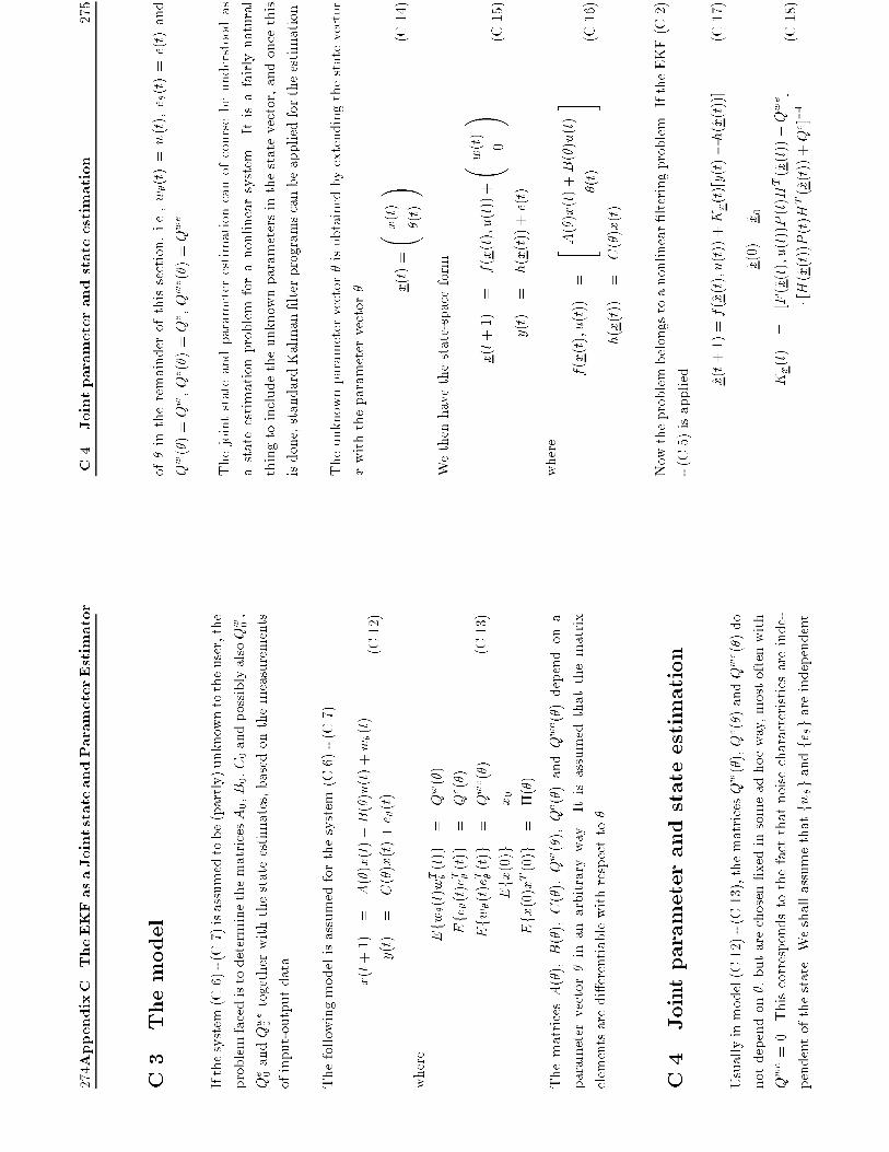
274AppendixC.TheEKFasaJointstateandParameterEstimator

C.3

Themodel

Ifthesystem(C.6)-(C.7)isassumedtobe(partly)unknowntotheuser,the

problemfacedistodeterminethematricesA0,B0,C0andpossiblyalsoQw 0,

Qe 0andQwe0

togetherwiththestateestimates,basedonthemeasurements

ofinput-outputdata.

Thefollowingmodelisassumedforthesystem(C.6)-(C.7)

x(t+1)

=

A(�)x(t)+B(�)u(t)+w�(t)

y(t)

=

C(�)x(t)+e �(t)

(C.12)

where

Efw�(t)wT �(t)g=

Qw(�)

Efe�(t)eT �(t)g=

Qe(�)

Efw�(t)eT �(t)g=

Qwe(�)

Efx(0)g=

x0

Efx(0)xT(0)g=

�(�)

(C.13)

ThematricesA(�),B(�),C(�),Qw(�),Qe(�)andQwe(�)dependona

parametervector�inanarbitraryway.Itisassumedthatthematrix

elementsaredi�erentiablewithrespectto�.

C.4

Jointparameterandstateestimation

Usuallyinmodel(C.12)-(C.13),thematricesQw(�),Qe(�)andQwe(�)do

notdependon�,butarechosen�xedinsomeadhocway,mostoftenwith

Qwe=0.Thiscorrespondstothefactthatnoisecharacteristicsareinde-

pendentofthestate.Weshallassumethatfw�gandfe�gareindependent

C.4

Jointparameterandstateestimation

275

of�intheremainderofthissection,i.e.,w�(t)=w(t),e �(t)=e(t)and

Qw(�)=Qw,Qe(�)=Qe,Qwe(�)=Qwe.

Thejointstateandparameterestimationcanofcoursebeunderstoodas

astateestimationproblemforanonlinearsystem.Itisafairlynatural

thingtoincludetheunknownparametersinthestatevector,andoncethis

isdone,standardKalman�lterprogramscanbeappliedfortheestimation.

Theunknownparametervector�isobtainedbyextendingthestatevector

xwiththeparametervector� x

(t)=

x(t)

�(t)

!

(C.14)

Wethenhavethestate-spaceform

x(t+1)

=

f(x(t);u(t))+

w(t)

0

!

y(t)

=

h(x(t))+e(t)

(C.15)

where

f(x(t);u(t))

=

" A(�)x(t)+B(�)u(t)

�(t)

#

h(x(t))

=

C(�)x(t)

(C.16)

Nowtheproblembelongstoanonlinear�lteringproblem.IftheEKF(C.2)

-(C.5)isapplied ^x

(t+1)=f(^x(t);u(t))+Kx(t)[y(t)�h(^x(t))]

(C.17)

^x(0)=^x0

Kx(t)

=

[F(^x(t);u(t))� P(t)HT(^x(t))+� Qwe]

�[H(^x(t))� P(t)HT(^x(t))+Qe]�1

(C.18)

276AppendixC.TheEKFasaJointstateandParameterEstimator

� P(t+1)

=

F(^x(t);u(t))� P(t)FT(^x(t);u(t))+� Qw

�Kx(t)[H(^x(t))� P(t)HT(^x(t))+Qe]KT x(t)

(C.19)

� P(0)=

� P0

where

F(^x(t);u(t))

=

@ @xf(x;u)� � � x=^x(t)

=

" A(^ �(t))

M(^ �(t);^x(t);u(t))

0

I

#

(C.20)

H(^x(t))

=

@ @xh(x)� � � x=^x(t)

=

[C(^ �(t))D(^ �(t);^x(t))]

(C.21)

� Qw

=

" Qw

0

0

0#

� Qwe

=

" Qwe

0

#

(C.22)

^x0

=

" ^x0 ^ � 0

#

� P0

=

�(^ �0)

0

0

�0

!

(C.23)

Here

M(^ �(t);^x(t);u(t))=

@ @�

(A(�)^x(t)+B(�)u(t))

� � � � �=^ �(t)

(C.24)

D(^ �(t);^x(t))=

@ @�

(C(�)^x(t))

� � � � �=^ �(t)

(C.25)

^ � 0and�0representsomeaprioriinformationabouttheparametervector

�.

C.4

Jointparameterandstateestimation

277

Introduceforshort

At=A(^ �(t))

Bt=B(^ �(t))

Ct=C(^ �(t))

Dt=D(^ �(t);^x(t))

Mt=M(^ �(t);^x(t);u(t))

IfwewritematricesKx(t)and� P(t)intheform

Kx(t)=

" Kx(t)

K�(t)

#

� P(t)=

" P1(t)

P2(t)

PT 2(t)

P3(t)

#

equations(C.17)canthenberewrittenexplicitlyas

^x(t+1)=At^x(t)+Btu(t)+Kx(t)[y(t)�Ct^x(t)]

(C.26)

^x(0)=^x0

and

^ �(t+1)=^ �(t)+K�(t)[y(t)�Ct^x(t)]

(C.27)

^ �(0)=^ � 0

Rewritingtheequation(C.18)as

Kx(t)

K�(t)

! = "At

Mt

0

I

#"P1(t)

P2(t)

PT 2(t)

P3(t)

#"CT t

DT t

# +" Qwe

0

#! �S�1

278AppendixC.TheEKFasaJointstateandParameterEstimator

where

St=[Ct

Dt]" P

1(t)

P2(t)

PT 2(t)

P3(t)

#"CT t

DT t

# +Qe

Kx(t)andK�(t)canthenbeobtained

Kx(t)=[AtP1(t)CT t

+MtPT 2(t)CT t

+AtP2(t)DT t

+MtP3(t)DT t

+Qwe]S�1t

(C.28)

K�(t)=[PT 2(t)CT t

+P3(t)DT t]S�1t

(C.29)

and S

t=CtP1(t)CT t

+CtP2(t)DT t

+DtPT 2(t)CT t

+DtP3(t)DT t

+Qe

(C.30)

Inthesamewaytheequation(C.19)isrewrittenas

P1(t+1)

P2(t+1)

PT 2(t+1)

P3(t+1)

! =" A

t

Mt

0

I

#"P1(t)

P2(t)

PT 2(t)

P3(t)

#"AT t

0

MT t

I#

+" Qw

0

0

0# �" K

x(t)

K�(t)

# St[KT x(t)KT �(t)]

ThematricesP1(t),P2(t)andP3(t)canbeobtained

P1(t+1)=AtP1(t)AT t+AtP2(t)MT t

+MtPT 2(t)AT t+MtP3(t)MT t

�Kx(t)StKT x(t)+Qw

(C.31)

P1(0)=�0(^ �0)

C.4

Jointparameterandstateestimation

279

P2(t+1)=AtP2(t)+MtP3(t)�Kx(t)StKT �(t)

(C.32)

P2(0)=0

P3(t+1)=P3(t)�K�(t)StKT �(t)

(C.33)

P3(0)=�0

ByinsertingmatrixK�(t)intoequation(C.32),P2(t+1)canberewritten

as

P2(t+1)=(At�Kx(t)Ct)P2(t)+(Mt�Kx(t)Dt)P3(t)

(C.34)

Itcouldbementionedthatcertainnumericalproblemswillariseinthealgo-

rithmifMt�Kx(t)Dtisnotafullrankstochasticprocess(i.e.,itscovariance

matrixissingular).Thisaquestionassociatedwiththeparameterizationof

themodel(C.12).Insuchacase,weshallinthesequelassumethatsome

measuresaretakentocomearoundthesenumericalproblems.Asimple

wayistoreplace(C.33)by

P3(t+1)=[fP3(t)�K�(t)StKT �(t)g�1+�I]�

1

(C.35)

forsomesmallpositive�.Noticethatforsmall�,(C.35)canbeapproxi-

matedby

P3(t+1)=P3(t)�K�(t)StKT �(t)��P3(t)P3(t)

(C.36)

280AppendixC.TheEKFasaJointstateandParameterEstimator

C.5

Convergenceanalysis

Convergenceofthealgorithm(C.26)-(C.33)willbeanalysedusingthe

ordinarydi�erentialequation(ODE)methodwhichisdevelopedbyLjung.

Weshallinthissectiondeterminethedi�erentialequationthatisassociated

withthealgorithm(C.26)-(C.33).

Thedi�erentialequationisde�nedintermsoftheprocessthat(C.26)-

(C.33)wouldproduceifthemodelparameterswerekeptconstant=�.This

meansthat(C.27)wouldbereplacedby^ �(t)=�.Consequentlyinthe

�-dependentmatrices[At;Bt;Ct;MtandDt]theestimate^ �(t)shouldbe

replacedby�.ItiseasytoseethatP2andP3wouldtendtozeroand

� P1(�)=A(�)� P1(�)AT(�)+Qw�� Kx(�)� S(�)� KT x(�)

(C.37)

� S(�)=C(�)� P1(�)CT(�)+Qe

(C.38)

� Kx(�)=[A(�)� P1(�)CT(�)+Qwe]� S�1(�)

(C.39)

Thende�netheprocess� ^x(t;�)astheestimatesthatwouldbeobtainedwith

thisconstantmodel,correspondingtotheparametersvalue�

� ^x(t+1;�)=A(�)� ^x(t;�)+B(�)u(t)+� Kx(�)��(t;�)

(C.40)

where

��(t;�)=y(t)�C(�)� ^x(t;�)

(C.41)

ItisnaturaltointerprettheEKFasanattempttominimizetheexpected

valueofthesquaredresidualsassociatedwithmodel�.Asuitablecriterion

toseektominimizewouldbe V

(�)=Ej��(t;�)j2

(C.42)

C.5

Convergenceanalysis

281

AreasonableadjustmentschemetoachieveminimizationofV(�)shouldbe

relatedtothegradientofV(�)

d d�

V(�)=2E

��d d

���T(t;�)� ��(t;�)

�

(C.43)

Denotethematrix

�d d

���T(t;�)=

� (t;�)

(C.44)

ThenthenegativegradientofV(�)canbewritten

�d d

�V(�)=2E� (t;�)��(t;�)

(C.45)

theparametervaluesof�wouldbecorrectedinthisdirection.

Di�erentiating(C.41)gives

d d�

��(t;�)=�

� d d�

C(�)� � ^x(t;�)�C(�)

� d d�

� ^x(t;�)�

(C.46)

whered=d�� ^x(t;�)canbefoundbydi�erentiating(C.40)

d d�

� ^x(t+1;�)=[A(�)�� Kx(�)C(�)]

d d�

� ^x(t;�)+

� d d�

A(�)� � ^x(t;�)

+� d d

�B(�)� u(t)�� Kx(�)

� d d�

C(�)� � ^x(t;�)

(C.47)

+� d d

�� Kx(�)� ��(t;�)

Furthermorewede�ne�w(t;�)=d=d�� ^x(t;�)

�w(t+1;�)=[A(�)�� Kx(�)C(�)]�w(t;�)

+[M(�;� ^x(t;�);u(t))�� Kx(�)D(�;� ^x(t;�))]

(C.48)

+� d d

�� Kx(�)� ��(t;�)

282AppendixC.TheEKFasaJointstateandParameterEstimator

andthen� (t;�)canbefound

� (t;�)=[C(�)�w(t;�)+D(�;� ^x(t;�))]T

(C.49)

wherematricesM

andDwerede�nedby(C.24)and(C.25).

Ifweremovethecolumn[d=d�� Kx(�)]��(t;�)from

�w(t+1;�)(thereason

willbeshownlater)andcompareitwith(C.34),itcanbeeasilyfoundthat

P2��w(t;�)~ P3forgivenconstant�.Again,bycomparing� (t;�)withK�(t),

havinginmindthatP2��w(t;�)~ P3,weseethatK�(t)�~ P3� (t;�)� S�1(�)

forgivenconstant�and~ P3.

Since,accordingto(C.27)andthede�nitionofODEinAppendix

B,it

seemsreasonablethat

f(�)=E� (t;�)� S�1(�)��(t;�)

(C.50)

whereEdenotesexpectationwithrespecttothestochasticprocessy(t)and

u(t).De�nealso

G(�)=E� (t;�)� S�1(�)� T(t;�)

(C.51)

wemaythusinterpretf(�)asthedirection(modi�edbyR�1

=

~ P3)in

whichtheestimatesasymptoticallyareadjusted.

Whatwehavedoneuntilnowistogiveaformalde�nitionofthefunctions

f(�)andG(�).ThustheODEcanbeobtainedby

d d�

�(�)=R�1(�)f(�(�))

d d�

R(�)=G(�(�))+�I�R(�)

(C.52)

if�(t)convergesto��(��isastationarypointofthedi�erentialequation),

then

f(�� )=0

C.5

Convergenceanalysis

283

R�=G(�� )+�I

(C.53)

Now,asseenfrom

thede�nitionoff(�)in(C.50),thisfunctionisthe

correlationbetweentheresiduals(innovations)��(t;�)obtainedfrommodel

�andvariable� (t;�).Thisrandom

variableisaccordingto(C.48)and

(C.49)obtainedbylinear�lteringofthestateestimatescorrespondingto

thesamemodel�.Thereforef(�)isameasureofthecorrelationbetween

thecurrentinnovationandpreviousstateestimates,whichinturncanbe

obtainedfrompreviousresiduals.Therefore,itisclearthatf(�)measures

thecorrelationofthesequencef��(t;�)g.

Ifthesequencef��(t;�)gisuncorrelatedforsome�=��,thenf(�� )=0

and�=

��,R

=

G(�� )+�Iisastationarypointof(C.52).However,

theconverseisnotnecessarilytrue,i.e.,f(�� )=

0doesnotingeneral

implythatf��(t;�� )gisasequenceofuncorrelatedrandom

vectors.The

problemiscausedbythatwehaveremovedthecolumn[d=d�� Kx(�)]��(t;�)

from

�w(t+1;�),whenwediscusstheconvergencepropertiesoftheEKF.It

meansthatonlyinthespecialcasewhere� Kx(�)happenstobeindependent

of�,i.e.,[d=d�� Kx(�)]=0,theconvergencepropertiesoftheEKFcanbe

satis�ed.Thiscanbeexplainedbelow.

Supposethatforsome� 0,

A0=A(�0)

B0=B(�0)

C0=C(�0)

(C.54)

wherematricesA0,B0

andC0

arethetruesystem

matrices,whichare

obtainedforacertainparametervector� 0.Thenf��(t;�0)gwillbeingeneral

284AppendixC.TheEKFasaJointstateandParameterEstimator

anorthogonalsequenceonlyif

� K0=

� Kx(�0)

(C.55)

where� K0isde�nedby(C.11)and� Kx(�0)by(C.39).Thisconditionholds

onlyiftheassumptionsaboutnoisestructureofthemodel(C.13)arein

accordancewiththoseofthetruesystem(C.7).Consequently,avalue� 0

correspondingtothetruesystem

willingeneralbeastationarypointof

(C.52)andhenceapossibleconvergencepointonlyiftheassumednoise

structurecoincideswiththetrueone.Otherwisetheestimateswillbebi-

ased.

Itisofcoursesomewhatunrealistictoassumethatthenoisestructureofthe

systemisknown,whilethedynamicsofthesystemareunknown.However

wemightexpecttheimprovedasymptoticconvergencepropertiesofthe

EKFif[d=d�� Kx(�)]�(t),where�(t)isthecurrentresidual,isaddedtothe

matrixMtinthealgorithm(C.26)-(C.33).Ljunginhispaper[Ljung79b]

givesamodi�edalgorithmandaGauss-Newtonalgorithmbyusinginnova-

tionsmodel.Thesetwoalgorithmshavethesameasymptoticconvergence

properties.TheGauss-Newtonalgorithmcouldbecalledarecursivepre-

dictionerroralgorithmwhichisgivenisAppendixD.

AppendixD

TheRPEMethodApplied

totheInnovationsModel

Therecursivepredictionerror(RPE)methodappliedtoaninnovations

modelisgivenbyLjunginhisbookTheoryandPracticeofRecursiveIden-

ti�cation[LjungandS�oderstr�om83].

D.1

Themodel

Thee�ectoftheassumptionsassociatedwiththenoisecovariancematrices

Qw(�),Qe(�)andQwe(�)instate-spacemodel(C.12)-(C.13)inAppendix

CisinfactonlytoprovidetheKalman�ltergain.Itisthisgainthathas

thealgorithmicimportance.Thenoiseassumptionsareonlythevehiclesto

285

286AppendixD.TheRPEMethodAppliedtotheInnovationsModel

arriveatit.Thereforeinmostcasesitshouldbeagoodideatoparameterize

thesteady-stateKalmangainratherthanthecovariancematrices.This

willnormallyinvolvefewerparameters.Theonlycases,whenthismaybe

undesirableiswhenimportantaprioriinformationofthenoisestructurein

themodel(C.12)isavailableorwhenitisimportanttohaveatime-varying

Kalmangainfortheinitialpartoftherecordeddata[Ljung79b].

Aninnovationsmodelis

x(t+1)

=

A(�)x(t)+B(�)u(t)+Kx(�)�(t)

y(t)

=

C(�)x(t)+�(t)

(D.1)

with

Ex(0)=x0(�)

E[x(0)�x0(�)][x(0)�x0(�)]T

=�(�)

where�(t)isthepredictionerrororinnovationy(t)�^y(tj�)withvariance

Ef�(t)�T(s)g=�� ts

(D.2)

Insteadofmodel(C.12)-(C.13)inAppendixC,thevariancematricesare

Qw(�)=Kx(�)�KT x(�)

Qe(�)=�

(D.3)

Qwe(�)=Kx(�)�

D.2

Thealgorithm

Thepredictionoftheoutputforthemodel(D.1)-(D.2)isobtainedby

^x(t+1)

=

A(�)^x(t)+B(�)u(t)+Kx(�)�(t;�)

^y(tj�)=

C(�)^x(t)

(D.4)

D.2

Thealgorithm

287

with

^x(0)=^x0

andthepredictionerroris

�(t;�)=y(t)�^y(tj�)

(D.5)

Arecursivealgorithm

isderivedforestimationofmodelparametersby

minimizingapredictionerrorcriterion

V(�)=E

1 2�T(t;�)��1�(t;�)

(D.6)

where�isapositivede�nitecovariancematrix.

The�rstderivativeofthecriterionis

� d d�

V(�)� T =

� d d�

�(t;�)

� T ��1�(t;�)

(D.7)

where

d d�

�(t;�)=

d d�

[y(t)�^y(tj�)]=�

d d�

^y(tj�)=� T(t;�)

(D.8)

ThesecondderivativeofV(�)(theHessian)canbeapproximatedby

d2

d�2

V(�)�E (t;�)��1 (t;�)

(D.9)

AnapproximationoftheHessianisoftenreferredtoastheGauss-Newton

direction,whichguaranteespositivesemide�nite.

IfwedenotethesecondderivativeapproximationbyR(t),theGauss-Newton

iterationbecomes

^ �(t)=^ �(t�1)+ (t)R(t)�1 (t)��1�(t)

(D.10)

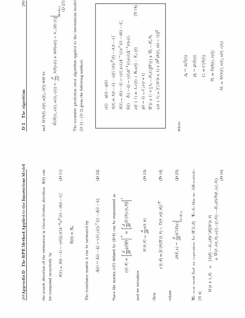
288AppendixD.TheRPEMethodAppliedtotheInnovationsModel

thesearchdirectionoftheestimationisGauss-Newtondirection.R(t)can

becomputedrecursivelyby

R(t)=R(t�1)+ (t)[ (t)��1 T(t)�R(t�1)]

(D.11)

R(0)=R0

Thecovariancematrix�canbeestimatedby

^ �(t)=^ �(t�1)+ (t)[�(t)�T(t)�^ �(t�1)]

(D.12)

Sincethematrix (t)de�nedby(D.8)canberepresentedas

(t;�)=

� d d�

^y(tj�)

� T =� d d

�[C(�)^x(t;�)]

� T

andweintroduce

W(t;�)=

d d�

^x(t;�)

(D.13)

then

(t;�)=[C(�)W(t;�)+D(�;^x(t;�))]T

(D.14)

where

D(^ �;^x)=

@ @�

(C(�)^x)� � � � �=^ �

(t)

(D.15)

Wenowmust�ndanexpressionforW(t;�).Todothiswedi�erentiate

(D.4) W

(t+1;�)

=

[A(�)�Kx(�)C(�)]W(t;�)

+

� M(�;^x(t;�);u(t);�(t;�))�Kx(�)D(�;^x(t;�)) (D

.16)

D.2

Thealgorithm

289

and� M(^ �(t);^x(t);u(t);�(t))willbe

� M(^ �(t);^x(t);u(t);�(t))=

@ @�

[A(�)^x(t)+B(�)u(t)+Kx(�)�(t)]

� � � � �=^ �(t)

(D.17)

Therecursivepredictionerroralgorithmappliedtotheinnovationsmodel

(D.1)-(D.2)givesthefollowingmethod:

�(t)=y(t)�^y(t)

^ �(t)=^ �(t�1)+ (t)[�(t)�T(t)�^ �(t�1)]

R(t)=R(t�1)+ (t)[ (t)^ ��1(t) T(t)�R(t�1)]

^ �(t)=^ �(t�1)+ (t)R�1(t) (t)^ ��1(t)�(t)

^x(t+1)=At^x(t)+Btu(t)+Kt�(t)

(D.18)

^y(t+1)=Ct^x(t+1)

W(t+1)=[At�KtCt]W(t)+

� Mt�KtDt

(t+1)=[CtW(t+1)+DT(^ �(t);^x(t+1))]T

where

At=A(^ �(t))

Bt=B(^ �(t))

Ct=C(^ �(t))

Dt=D(^ �(t);^x(t))

� Mt=

� M(^ �(t);^x(t);u(t);�(t))

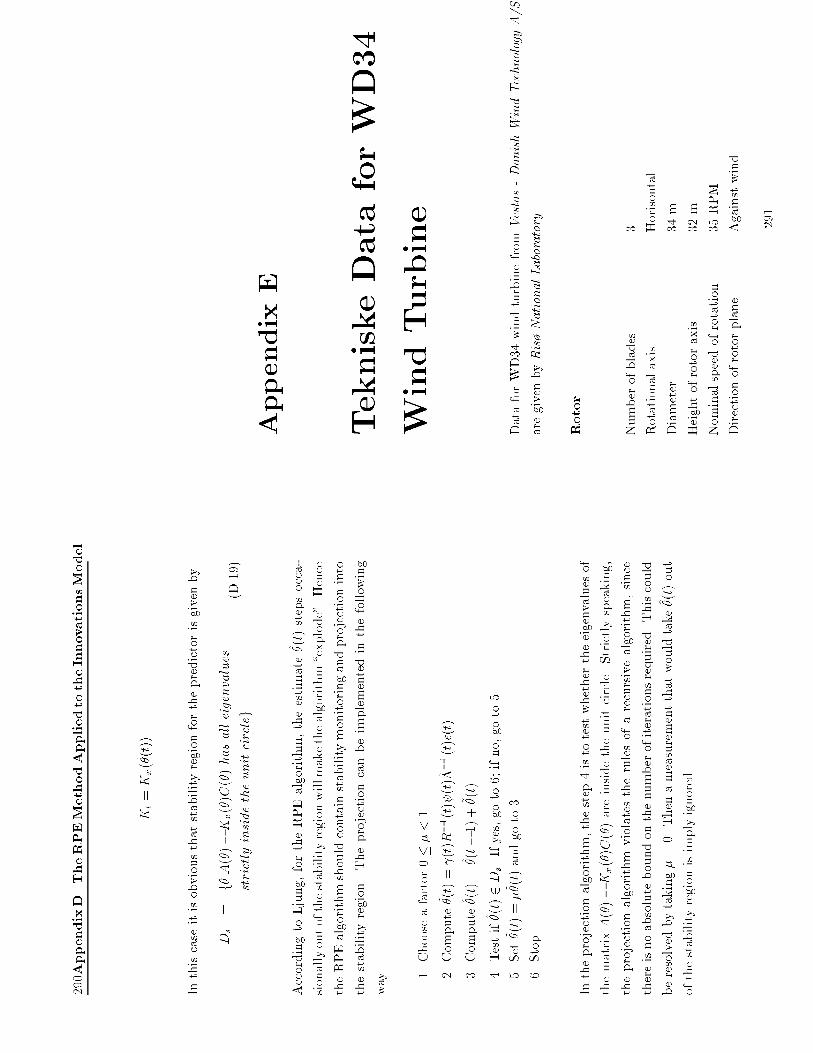
290AppendixD.TheRPEMethodAppliedtotheInnovationsModel

Kt=Kx(^ �(t))

Inthiscaseitisobviousthatstabilityregionforthepredictorisgivenby

Ds

=

f�jA(�)�Kx(�)C(�)hasalleigenvalues

strictlyinsidetheunitcircleg

(D.19)

AccordingtoLjung,fortheRPEalgorithm,theestimate^ �(t)stepsocca-

sionallyoutofthestabilityregionwillmakethealgorithm\explode".Hence

theRPEalgorithmshouldcontainstabilitymonitoringandprojectioninto

thestabilityregion.Theprojectioncanbeimplementedinthefollowing

way. 1.

Chooseafactor0��<1

2.Compute~ �(t)= (t)R�1(t) (t)^ ��1(t)�(t)

3.Compute^ �(t)=^ �(t�1)+~ �(t)

4.Testif^ �(t)2Ds.Ifyes,goto6;ifno,goto5

5.Set~ �(t)=�~ �(t)andgoto3

6.Stop

Intheprojectionalgorithm,thestep4istotestwhethertheeigenvaluesof

thematrixA(�)�Kx(�)C(�)areinsidetheunitcircle.Strictlyspeaking,

theprojectionalgorithmviolatestherulesofarecursivealgorithm,since

thereisnoabsoluteboundonthenumberofiterationsrequired.Thiscould

beresolvedbytaking�=0.Thenameasurementthatwouldtake^ �(t)out

ofthestabilityregionisimplyignored.

AppendixE

TekniskeDataforWD34

WindTurbine

DataforWD34windturbinefromVestas-DanishWindTechnologyA/S

aregivenbyRis�NationalLaboratory.

Rotor

Numberofblades

3

Rotationalaxis

Horisontal

Diameter

34m

Heightofrotoraxis

32m

Nominalspeedofrotation

35RPM

Directionofrotorplane

Againstwind

291

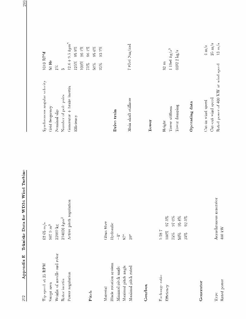
292

AppendixE.TekniskeDataforWD34WindTurbine

Tipspeedat35RPM

62.65m/s

Sweptarea

907.9m2

Weightofnacelleandrotor

21000kg

Rotorinertia

214000kgm2

Powerregulation

Activepitchregulation

Pitch

Material

Glass�ber

Bladerotationsystem

Hydraulic

Minimalpitchangle

�2o

Maximalpitchangle

87o

Maximalpitchrated

10o

Gearbox

Exchangeratio

1:28.7

E�ciency

100%

97.5%

75%

97.0%

50%

95.8%

25%

92.5%

Generator

Type

Asynchronousgenerator

Ratedpower

400kW

293

Synchronousangularvelocity

1010RPM

Gridfrequency

50Hz

Nominalslip

1%

Numberofpolepairs

3

Generator+brakeinertia

12:6+9:5kgm2

E�ciency

125%

95.9%

100%

96.1%

75%

96.1%

50%

95.6%

25%

93.2%

Drivetrain

Mainshaftsti�ness

7.87e6Nm/rad

Tower

Height

32m

Towersti�ness

1.19e6kg=s2

Towerdamping

4492.2kg/s

Operatingdata

Cut-inwindspeed

4m/s

Cut-outwindspeed

25m/s

Ratedpowerof400KW

atwindspeed

13m/s

294

AppendixE.TekniskeDataforWD34WindTurbine

295

Ph.D.thesesfrom

IM

M

1.Larsen,Rasmus.(1994).Estimationofvisualmotioninimage

sequences.xiv+143pp.

2.Rygard,JensMoberg.(1994).Designandoptimizationof exible

manufacturingsystems.xiii+232pp.

3.Lassen,NielsChristianKrieger.(1994).Automateddetermina-

tionofcrystalorientationsfromelectronbackscatteringpatterns.xv

+136pp.

4.Melgaard,Henrik.(1994).Identi�cationofphysicalmodels.xvii

+246pp.

5.Wang,Chunyan.(1994).Stochasticdi�erentialequationsanda

biologicalsystem.xxii+153pp.

6.Nielsen,AllanAasbjerg.(1994).Analysisofregularlyandirreg-

ularlysampledspatial,multivariate,andmulti-temporaldata.xxiv+

213pp.

7.Ersb�ll,AnnetteKj�r.(1994).Onthespatialandtemporalcorre-

lationsinexperimentationwithagriculturalapplications.xviii+345

pp.

8.M�ller,Dorte.(1994).Methodsforanalysisanddesignofhetero-

geneoustelecommunicationnetworks.Volume1-2,xxxviii+282pp.,

283-569pp.

9.Jensen,JensChristian.

(1995).

Teoretiskeogeksperimentelle

dynamiskeunders�gelserafjernbanek�ret�jer.ATVErhvervsforsker-

projektEF435.viii+174pp.

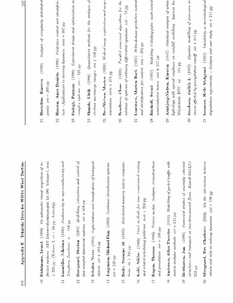
296

AppendixE.TekniskeDataforWD34WindTurbine

10.Kuhlmann,Lionel.(1995).Onautomaticvisualinspectionofre-

ectivesurfaces.ATVErhvervsforskerprojektEF385.Volume1,xviii

+220pp.,(Volume2,vi+54pp.,fortrolig).

11.Lazarides,Nikolaos.(1995).Nonlinearityinsuperconductivityand

JosephsonJunctions.iv+154pp.

12.Rostgaard,Morten.(1995).Modelling,estimationandcontrolof

fastsampleddynamicalsystems.xiv+348pp.

13.Schultz,Nette.(1995).Segmentationandclassi�cationofbiological

objects.xiv+194pp.

14.J�rgensen,MichaelFinn.(1995).NonlinearHamiltoniansystems.

xiv+120pp.

15.Balle,SusanneM.(1995).Distributed-memorymatrixcomputa-

tions.iii+101pp.

16.Kohl,Niklas.(1995).Exactmethodsfortimeconstrainedrouting

andrelatedschedulingproblems.xviii+234pp.

17.Rogon,Thomas.(1995).Porousmedia:Analysis,reconstruction

andpercolation.xiv+165pp.

18.Andersen,AllanTheodor.(1995).Modellingofpackettra�cwith

matrixanalyticmethods.xvi+242pp.

19.Hesthaven,Jan.(1995).Numericalstudiesofunsteadycoherent

structuresandtransportintwo-dimensional ows.Ris�-R-835(EN)

203pp.

20.Slivsgaard,EvaCharlotte.(l995).Ontheinteractionbetween

wheelsandrailsinrailwaydynamics.viii+196pp.

297

21.Hartelius,Karsten.

(1996).

Analysisofirregularlydistributed

points.xvi+260pp.

22.Hansen,AncaDaniela.(1996).Predictivecontrolandidenti�ca-

tion-Applicationstosteeringdynamics.xviii+307pp.

23.Sadegh,Payman.(1996).Experimentdesignandoptimizationin

complexsystems.xiv+162pp.

24.Skands,Ulrik.(1996).Quantitativemethodsfortheanalysisof

electronmicroscopeimages.xvi+198pp.

25.Bro-Nielsen,Morten.(1996).Medicalimageregistrationandsurge r

simulation.xxvii+274pp.

26.Bendtsen,Claus.(1996).Parallelnumericalalgorithmsforthe

solutionofsystemsofordinarydi�erentialequations.viii+79pp.

27.Lauritsen,MortenBach.(1997).Delta-domainpredictivecontrol

andidenti�cationforcontrol.xxii+292pp.

28.Bischo�,Svend.

(1997).ModellingColliding-pulsemode-locked

semiconductorlasers.xxii+217pp.

29.Arnbjerg-Nielsen,Karsten.(1997).Statisticalanalysisofurban

hydrologywithspecialemphasisonrainfallmodelling.Institutfor

Milj�teknik,DTU.xiv+161pp.

30.Jacobsen,JudithL.(1997).Dynamicmodellingofprocessesin

riversa�ectedbyprecipitationruno�.xix+215pp.

31.Sommer,HelleM�lgaard.(1997).Variabilityinmicrobiological

degradationexperiments.-Analysisandcasestydy.xiv+211pp.

298

AppendixE.TekniskeDataforWD34WindTurbine

32.Ma,Xin.(1997).Adaptiveextremumcontrolandwindturbinecon-

trol.xix+293pp.