XLME interpolants, a seamless bridge between XFEM and enriched

meshless methods

F. Amiri ∗ C. Anitescu † M. Arroyo ‡ S. P. A. Bordas§ T. Rabczuk ¶

Abstract

In this paper, we develop a method based on local maximum entropy (LME) shape functions togetherwith enrichment functions used in partition of unity methods to discretize problems in linear elasticfracture mechanics. We obtain improved accuracy relative to the standard extended finite elementmethod (XFEM) at a comparable computational cost. In addition, we keep the advantages of the LMEshape functions, such as smoothness and non-negativity. We show numerically that optimal convergence(same as in FEM) for energy norm and stress intensity factors can be obtained through the use ofgeometric (fixed area) enrichment with no special treatment of the nodes near the crack such as blendingor shifting.

Keywords: Local maximum entropy, Convex approximation, Meshless methods, Extrinsic enrichment

1 Introduction

Maximum entropy shape functions are a relatively new class of approximation functions, as they were firstintroduced in [1] in the context of polygonal interpolation. The idea of these functions is to maximize theShannon entropy [2] of the basis functions, which gives a measure of the uncertainty in the approximationscheme. The principle of maximum entropy (max-ent) was developed by Jaynes [3, 4], who showed thatthere is a natural correspondence between statistical mechanics and information theory. In particular,max-ent offers the least-biased statistical inference when the shape functions are viewed as probabilitydistributions subject to the approximation constraints (such as linear reproducing properties). However,without additional constraints, the basis functions are non-local, which due to increased overlapping makesthem unsuitable for analysis using Galerkin methods. The large overlapping of the basis functions, generallyleads to more expensive numerical integration due to large number of evaluation points. It also produces anon-sparse stiffness matrix, resulting in a linear system that is much more expensive to solve.

∗Institute of Structural Mechanics, Marienstr. 15, Bauhaus University Weimar, 99423, Germany. E-mail address:fatemeh.amiri@uni-weimar.de†Institute of Structural Mechanics, Marienstr. 15, Bauhaus University Weimar, 99423, Germany. E-mail address:

cosmin.anitescu@uni-weimar.de‡School of Civil Engineering of Barcelona (ETSECCPB), Departament de Matematica Aplicada 3, Universitat Politecnica

de Catalunya, Spain. E-mail address: marino.arroyo@upc.edu§Institute of Mechanics and Advanced Materials, Cardiff School of Engineering, Cardiff University, Queen’s Buildings, The

Parade, Cardiff, CF24 3AA Wales, UK. E-mail address: bordasS@cardiff.ac.uk¶Institute of Structural Mechanics, Marienstr. 15, Bauhaus University Weimar, 99423, Germany. Professor, School of Civil,

Environmental and Architectural Engineering, Korea University. E-mail address: timon.rabczuk@uni-weimar.de

1

The local maximum-entropy (LME) approximation schemes were developed in [5] using a frameworksimilar to meshfree methods. Here the support of the basis functions is introduced as a thermalization (orpenalty) parameter β in the constraint equations. When β = 0, then the max-ent principle is fully satisfiedand the basis functions will be least biased. For example, if only zero-order consistency is required, the shapefunctions are Shepard approximants [6] with Gaussian weight function. When β is large, then the shapefunctions have minimal support. In particular, they become the usual linear finite element functions definedon a Delaunay triangulation of the domain associated with the given node set. In [5] it was shown that forsome values of β, the approximation properties of the maximum-entropy basis functions are greatly superiorto those of the finite element linear functions, even when the added computational cost due to larger supportis taken into account.

Subsequent studies, such as [7, 8, 9], show that maximum entropy shape functions are suitable forsolving a variety of problems such as thin shell analysis, compressible and nearly-incompressible elasticityand incompressible media problems. Higher order approximations can also be obtained using the max-entframework, as shown in [10]. This class of methods is therefore related to the MLS-based meshless methods(due to the node-based formulation) and isogeometric analysis (with whom it shares features such as weakKronecker delta and non-negativity), inheriting some advantages from both.

In this work, we propose a coupling of the LME shape functions with the extrinsic enrichments used inpartition of unity enriched methods for fracture, such as the extended finite element method (XFEM), see[11, 12, 13].

There is a growing interest in modeling fracture mechanics with enrichment functions combined withmeshless methods [14, 15, 16], isogeometric analysis [17], or strain-smoothed FEM [18, 19]. Advantagesof the resulting methods include the possibility to model curved boundaries through higher order shapefunctions. The resulting basis functions also have higher continuity, which is particularly advantageouswhen the model problem requires it, such as the Kirchhoff-Love theory. Also in some enriched meshlessmethods, no representation of the crack’s topology is needed as this is handled through cracking particles asin [20] or weight-function enrichments as in [21, 22].

Here, we show that the enriched maximum entropy shape functions are suitable for this class of problems.Moreover, this method is more accurate than standard XFEM and does not require the so-called blendingelements (the elements near the crack tip). When compared to usual meshfree methods for crack propaga-tion, such as Element Free Galerkin (EFG), the method presented here can more easily deal with essentialboundary conditions, due to the fact that the shape functions satisfy a weak Kronecker delta property.The shape functions are also very smooth (C∞), which results in an accurate numerical integration with arelatively low number of integration points, especially for Gauss-Legendre quadrature [5, 8, 10]. Moreover,smooth and non-negative basis functions, such as those used in isogeometric analysis are gaining impetus.

The paper is organized as follows: in the next section we will briefly describe the LME approximants.Then we will introduce the coupling between LME and XFEM, with particular reference to implementationissues such as numerical integration. Next we examine the accuracy of the method through several numericalexamples, which indicate that the convergence rates for the energy norm of the error and the stress-intensityfactors, are O(h) and O(h2) respectively. Some concluding remarks are stated in the last section.

2 Local Maximum Entropy (LME) Approximants

LME meshfree approximants, introduced in [5], are related to other convex approximation schemes, such asnatural neighbor approximants [23], subdivision approximants [24], or B-spline and NURBS basis functions[25]. The LME basis functions will be denoted by pa(x), a = 1, ..., N with x ∈ Rd, d is the dimension

2

of the physical domain. They are non-negative and are required to satisfy the zeroth-order and first-orderconsistency conditions:

pa(x) ≥ 0, (1)N∑a=1

pa(x) = 1, (2)

N∑a=1

pa(x)xa = x. (3)

In the last equation, the vector xa identifies the positions of the nodes associated with each basis function.Consider a set of nodes X = xaa=1,...,N , which we will call the node set. The convex hull of X is the set

convX := x ∈ Rd|x = Xλ, λ ∈ RN+ ,1 · λ = 1 (4)

Here RN+ is the non-negative orthant, 1 denotes the vector in RN whose entries are one, and X is the d×Nmatrix whose columns are the co-ordinates of the position vectors of the nodes in the node set X [5]. Convexapproximants, which are in the span of convex basis functions, can only exist within the convex hull of X(orsubsets of it) and satisfy a weak Kronecker delta property at the boundary of the convex hull of the nodes.This means that the shape functions corresponding to the interior nodes vanish on the boundary. With thisproperty, the imposition of essential boundary conditions in the Galerkin method is straightforward.

The principle of maximum entropy comes from statistical physics and information theory, which considerthe measure of uncertainty or information entropy [2]. Consider a random variable χ : I → Rd, where Iis the index set I = 1, ..., N and χ(a) = xa gives to each index the position vector of its correspondingnode. Since the shape functions of a convex approximation scheme are non-negative and add to one, weregard p1(x), ..., pN (x) as the corresponding probabilities. The statistical expectation or average of thisrandom variable, as regarding equation (3), is x. According to this interpretation, the approximation of a

function u(x) ≈∑Na=1 pa(x)ua from the nodal values uaa=1,...,N is understood as an expected value u(x)

of a random variable µ : I → R where µ(a) = ua.The main idea of max-ent is to maximize the Shannon’s entropy, H(p1, p2, ..., pN ), subject to the consis-

tency constraints as follows:

(ME) For a fixed x maximize (5)

H(p1, p2, ..., pN ) = −N∑a=1

pa log(pa)

subject to pa ≥ 0, a = 1, ..., NN∑a=1

pa = 1

N∑a=1

paxa = x

Solving the (ME) problem produces the set of basis functions, pa := pa(x), a = 1, ..., N . However, these basisfunctions are non-local, i.e. they have support in all of convX, and are not suitable for use in a Galerkin

3

approximation because it would lead to a full, non-banded matrix. Nevertheless, they have been used in [1]as basis functions for polygonal elements.

Another optimization problem which takes into account the locality of the shape functions is Rajan’sform of the Delaunay triangulation [26]. This can be stated as the following linear program:

(RAJ) For a fixed x minimize (6)

U(x, p1, p2, ..., pN ) =

N∑a=1

pa |x− xa|2

subject to pa ≥ 0, a = 1, ..., NN∑a=1

pa = 1

N∑a=1

paxa = x

It is easy to see that U(x, p1, p2, ..., pN ) is minimized when the shape functions p1, ..., pN decay rapidly as thedistance from the corresponding nodes xa increases. There, the shape functions that satisfy (RAJ) problemwill have small supports, where the support can be defined up to a small tolerance ε by

supp(pa) = x : pa(x) > ε

The main idea of LME approximants is to compromise between the (ME) problem and the (RAJ) problemby introducing parameters βa that control the support of the pa. Therefore we write:

For a fixed x minimize (7)N∑a=1

βapa |x− xa|2 +

N∑a=1

pa log(pa)

subject to pa ≥ 0, a = 1, ..., NN∑a=1

pa = 1

N∑a=1

paxa = x

The non-negative parameters βa can in general be functions of the position x. This convex optimizationproblem is solved efficiently by a duality method as described in [5]. Finally, the shape functions are writtenin the form:

pa(x) =1

Z(x, λ∗(x))exp[−βa |x− xa|2 + λ∗(x) · (x− xa)]

where

Z(x, λ) =

N∑b=1

exp[−βb |x− xb|2 + λ · (x− xb)]

4

is a function associated with the node set X and λ∗(x) is defined by

λ∗(x) = arg minλ∈Rd

log Z(x, λ)

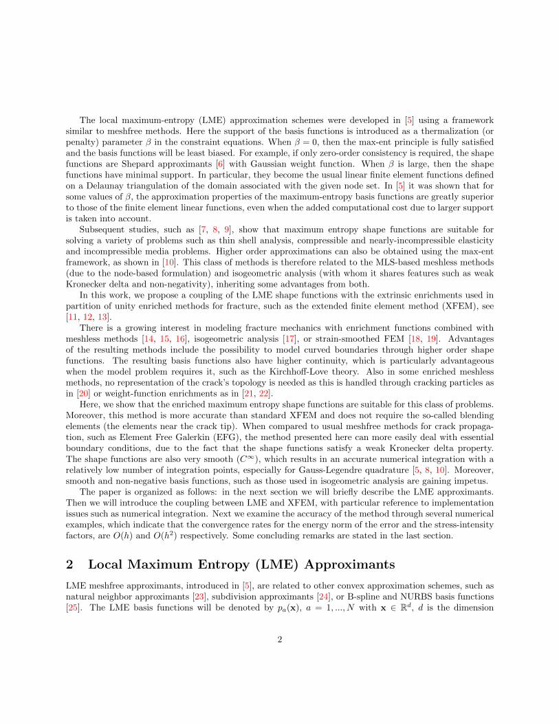
The local max-ent shape functions are as smooth as β(x) and pa(x, βa) is a continuous function of β ∈[0,+∞) [5]. For example LME shape functions are C∞ if β is constant. In this paper we choose β = γ

h2 ,where h is a measure of the nodal spacing and γ is constant over the domain. In this case the shape functionsare smooth and their degree of locality is controlled by the parameter γ. A plot of the LME functions forγ = 1.8 and a particular choice of nodes is given in Figure 1. In general, the optimal β is not obvious andthis will be discussed later in this paper.As we mentioned before, LME shape functions satisfy a weak Kronecker delta property at the boundary of

Figure 1: Local max-ent shape functions in 2D.

the convex hull of the nodes. Therefore, the shape functions that correspond to interior nodes vanish on theboundary.

3 Brief on extrinsic enrichments for Partition of Unity Methods

3.1 Description

The main idea of Partition of Unity (PU) enrichment as used here is to extend the max-ent approximationspace with some additional enrichment functions. The proposed method is based on a local partition of unityand uses an extrinsic enrichment to model the discontinuity. The max-ent approximation can be decomposed

5

into a standard part and an enriched part:

uh(x) =∑I∈W

pI(x)uI +∑J∈Wb

pJ(x)χ(φ(x))aJ+

∑K∈Ws

pK(x)

4∑k=1

Bk(x)bkK

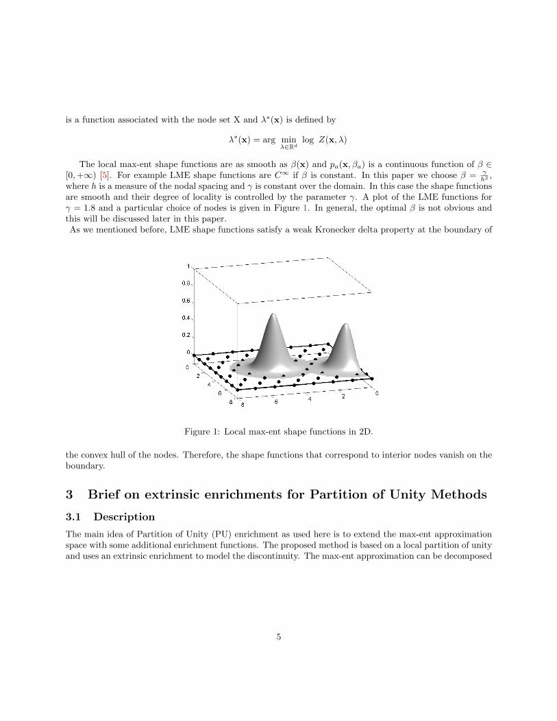
Here the first term is the standard approximation part and the second and the third terms are the enrichedparts. W is the set of nodes in the entire discretization and Wb and Ws are the sets of enriched nodes.pI are the shape functions and χ and Bk are the enrichment functions. Normally, χ is selected as a stepor Heaviside function and is used to enrich the nodes where the supports of the LME shape functions arecompletely cut by the crack. Bk are branch functions and are used to enrich the shape functions whosesupports include the crack tip. In this paper we use a geometric (fixed area) enrichment, and therefore weobtain optimal convergence rate (O(h2)) without a special treatment of the so-called ”blending” area aroundthe crack tip. Branch functions are defined as follows (in polar coordinate relative to the crack tip):

B1(r, θ) =√r sin

θ

2(8)

B2(r, θ) =√r cos

θ

2(9)

B3(r, θ) =√r sin

θ

2cos θ (10)

B4(r, θ) =√r cos

θ

2cos θ, (11)

where r =∥∥x− xtip

∥∥.φ(x) is the signed distance from the point x to the crack segment and aI and bkI are additional degrees

of freedom [27]. The signed distance function is defined as:

φ(x) = minxΓ∈Γ

‖x− xΓ‖ sign(n · (x− xΓ))

Here Γ is the curve of discontinuity, xΓ is an arbitrary point on Γ and n is normal vector to Γ (see Figure2). If we choose χ as a Heaviside function, then

H(φ(x)) =

1 if φ(x) > 0

−1 if φ(x) < 0(12)

This enrichment function captures the jump across the crack faces.In order to model a curved crack, the signed distance function can be approximated by the same shape

functions as the displacement. Assume t is a vector tangent to the curved crack, directed towards the cracktip. We approximate φ by:

φ(x) =∑I

pI(x)φI , x ∈ Ωφ (13)

Here φI are the nodal values of φ, pI are the shape functions and Ωφ, is the domain of definition for φ, givenby:

Ωφ := x|t · ∇r(x) > 0 (14)

6

Figure 2: Signed distance function.

So, the approximated crack position is considered as:

Γ := x|φ(x) = 0,x ∈ Ωφ (15)

In this case, φ(x) is not defined beyond the crack tip. So, two possibilities are considered for the angle θ ofthe Branch functions. If t · ∇r ≤ 0, then the regular polar angle from −t is computed. If t · ∇r > 0, θ isconsidered as in [28]:

θ = arctan(−φ√r2 − φ2

) (16)

3.2 Numerical Integration

3.2.1 Numerical Integration for LME

The numerical integration of LME shape functions poses similar challenges as that of the shape functionsused in meshless methods. In particular, the integrands used in the assembly of the stiffness matrix are non-polynomial and (depending on the values of the parameter γ) the supports of the shape functions overlapmore than in standard finite elements. However, the shape functions are smooth so only a relatively smallnumber of integration points are required.

In the examples we considered, we used quadrilateral background integration cells for integrating theshape functions whose support does not intersect the crack. For the values of γ between 4.8 and 1.8, andfor uniformly spaced nodes and square we found that the 4× 4 Gauss quadrature rule is sufficient to ensureoptimal convergence. Moreover, a quadrature rule with 8×8 Gauss points provides close to exact integration(i.e. the results change by less than 10−6 when the number of Gauss points is further increased).

3.3 Numerical Integration for Enriched LME

The usual numerical integration methods, for example Gauss quadrature, are less accurate for PU-enrichedmethods for fracture. This happens due to the discontinuity along the crack, and the singularity at the cracktip. The usual rule is to use a simple splitting of integration cells crossed by the crack [29]. In [30], a methodwas proposed in which each part of the elements that are cut or intersected by a discontinuity is mappedonto the unit disk using a conformal Schwarz-Christoffel map. However, for straight cracks, a triangulation

7

of the elements cut by the crack which takes into account the location of the discontinuity is relatively easyto implement and was used in this work.

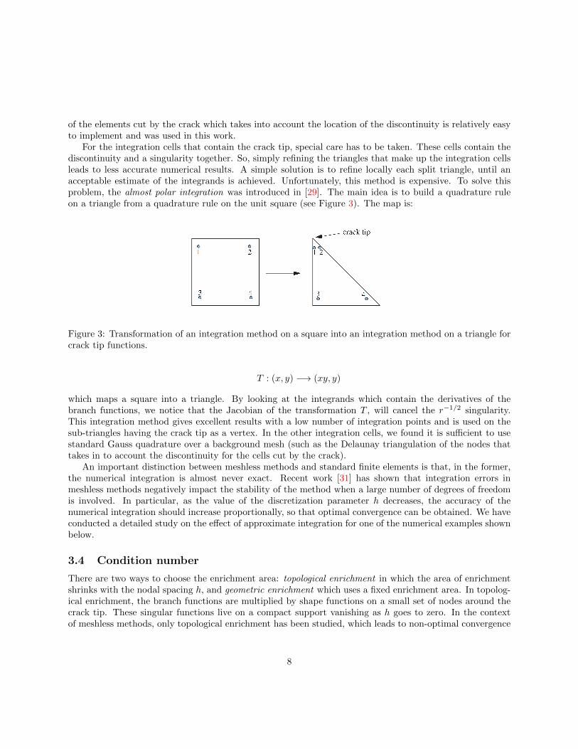
For the integration cells that contain the crack tip, special care has to be taken. These cells contain thediscontinuity and a singularity together. So, simply refining the triangles that make up the integration cellsleads to less accurate numerical results. A simple solution is to refine locally each split triangle, until anacceptable estimate of the integrands is achieved. Unfortunately, this method is expensive. To solve thisproblem, the almost polar integration was introduced in [29]. The main idea is to build a quadrature ruleon a triangle from a quadrature rule on the unit square (see Figure 3). The map is:

Figure 3: Transformation of an integration method on a square into an integration method on a triangle forcrack tip functions.

T : (x, y) −→ (xy, y)

which maps a square into a triangle. By looking at the integrands which contain the derivatives of thebranch functions, we notice that the Jacobian of the transformation T , will cancel the r−1/2 singularity.This integration method gives excellent results with a low number of integration points and is used on thesub-triangles having the crack tip as a vertex. In the other integration cells, we found it is sufficient to usestandard Gauss quadrature over a background mesh (such as the Delaunay triangulation of the nodes thattakes in to account the discontinuity for the cells cut by the crack).

An important distinction between meshless methods and standard finite elements is that, in the former,the numerical integration is almost never exact. Recent work [31] has shown that integration errors inmeshless methods negatively impact the stability of the method when a large number of degrees of freedomis involved. In particular, as the value of the discretization parameter h decreases, the accuracy of thenumerical integration should increase proportionally, so that optimal convergence can be obtained. We haveconducted a detailed study on the effect of approximate integration for one of the numerical examples shownbelow.

3.4 Condition number

There are two ways to choose the enrichment area: topological enrichment in which the area of enrichmentshrinks with the nodal spacing h, and geometric enrichment which uses a fixed enrichment area. In topolog-ical enrichment, the branch functions are multiplied by shape functions on a small set of nodes around thecrack tip. These singular functions live on a compact support vanishing as h goes to zero. In the contextof meshless methods, only topological enrichment has been studied, which leads to non-optimal convergence

8

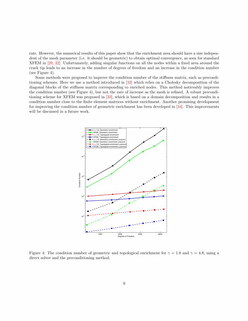
rate. However, the numerical results of this paper show that the enrichment area should have a size indepen-dent of the mesh parameter (i.e. it should be geometric) to obtain optimal convergence, as seen for standardXFEM in [29, 32]. Unfortunately, adding singular functions on all the nodes within a fixed area around thecrack tip leads to an increase in the number of degrees of freedom and an increase in the condition number(see Figure 4).

Some methods were proposed to improve the condition number of the stiffness matrix, such as precondi-tioning schemes. Here we use a method introduced in [32] which relies on a Cholesky decomposition of thediagonal blocks of the stiffness matrix corresponding to enriched nodes. This method noticeably improvesthe condition number (see Figure 4), but not the rate of increase as the mesh is refined. A robust precondi-tioning scheme for XFEM was proposed in [33], which is based on a domain decomposition and results in acondition number close to the finite element matrices without enrichment. Another promising developmentfor improving the condition number of geometric enrichment has been developed in [34]. This improvementswill be discussed in a future work.

1000 2000 4000 8000

104

106

108

1010

1012

Degrees of Freedom

Cond

itio

n N

um

be

r

γ = 1.8, Geometric enrichment

XFEM, Geometric enrichment

γ = 1.8, Topological enrichment

XFEM, Topological enrichment

γ = 1.8, Geometric enrichment, precond

XFEM, Geometric enrichment, precond

γ = 1.8, Topological enrichment, precond

XFEM, Topological enrichment, precond

Figure 4: The condition number of geometric and topological enrichment for γ = 1.8 and γ = 4.8, using adirect solver and the preconditioning method.

9

4 Numerical Examples

4.1 Infinite plate with a horizontal crack

Consider an infinite plate containing a straight crack of length 2a under a remote uniform stress field σ asshown in Figure 5. The analytical solution near crack tip for stress fields and displacement in terms of localpolar coordinates from the crack tip are [14]

σxx(r, θ) =KI√r

cosθ

2

(1− sin

θ

2sin

3θ

2

)σyy(r, θ) =

KI√r

cosθ

2

(1 + sin

θ

2sin

3θ

2

)σxy(r, θ) =

KI√r

sinθ

2cos

θ

2cos

3θ

2

ux(r, θ) =2(1 + υ)√

2π

KI

E

√r cos

θ

2

(2− 2υ − cos2 θ

2

)uy(r, θ) =

2(1 + υ)√2π

KI

E

√r sin

θ

2

(2− 2υ − cos2 θ

2

)where KI = σ

√πa is the stress intensity factor, υ is Poisson’s ratio and E is Young’s modulus.

Figure 5: Infinite plate with a center crack under uniform tension and modeled geometry ABCD.

The analytical solution is valid for region close enough to the crack tip. We consider a square ABCD oflength 10 mm × 10 mm, a = 100 mm, E = 107 N/mm

2, υ = 0.3, σ = 104 N/mm

2and the modeled crack

10

length is 5 mm. In all problems of this paper, plane strain state is assumed. We use Dirichlet boundaryconditions on the bottom, right and top edges and Neumann boundary conditions on the left edge whichincludes the crack. As we mentioned in Section 2, LME shape functions satisfy a weak Kronecker deltaproperty. This property allows us to impose Dirichlet boundary conditions by computing a node-basedinterpolant or an L2 projection of the boundary data. The latter can also be used for edges that containenriched nodes. Numerical integration is performed on a background mesh of rectangular elements and thealmost polar integration is used on the elements containing a crack tip.

10−0.9

10−0.7

10−0.5

10−0.3

10−5

10−4

10−3

10−2

h

Re

lative

err

or

γ = 0.8

γ = 1.8

γ = 2.8

γ = 3.8

γ = 4.8

XFEM

Slope 2

Figure 6: Error in the L2 norm for the horizontal crack problem.

11

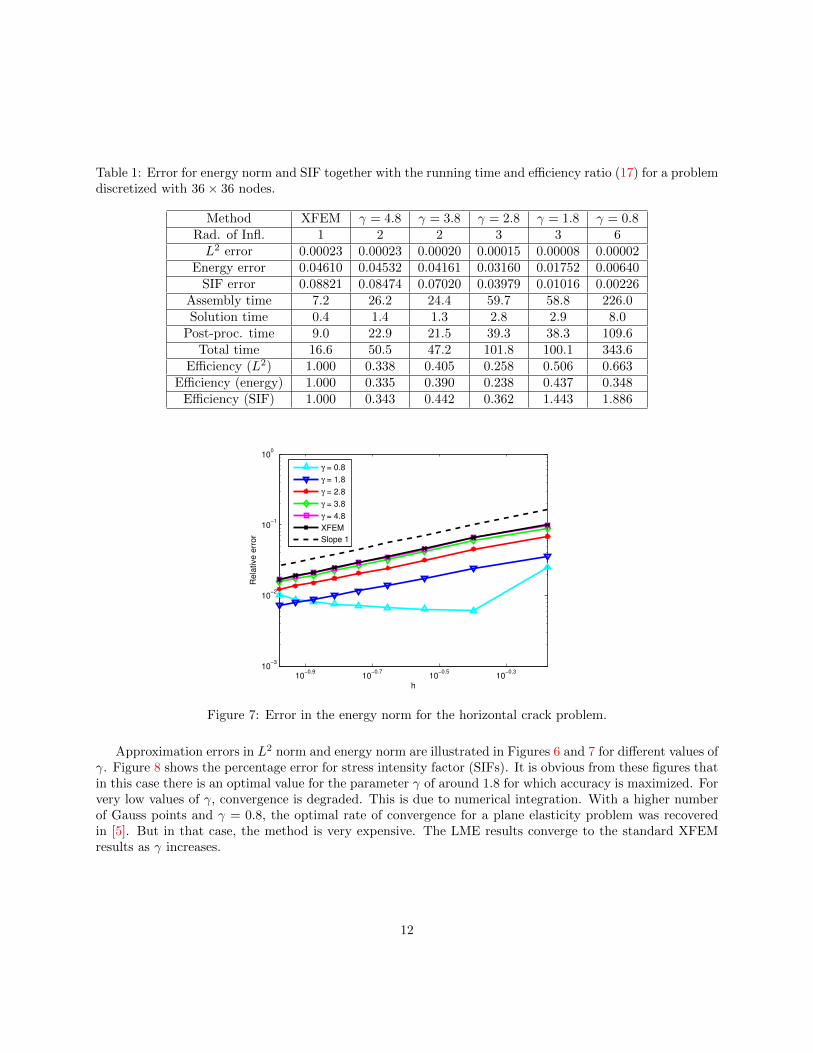
Table 1: Error for energy norm and SIF together with the running time and efficiency ratio (17) for a problemdiscretized with 36× 36 nodes.

Method XFEM γ = 4.8 γ = 3.8 γ = 2.8 γ = 1.8 γ = 0.8Rad. of Infl. 1 2 2 3 3 6L2 error 0.00023 0.00023 0.00020 0.00015 0.00008 0.00002

Energy error 0.04610 0.04532 0.04161 0.03160 0.01752 0.00640SIF error 0.08821 0.08474 0.07020 0.03979 0.01016 0.00226

Assembly time 7.2 26.2 24.4 59.7 58.8 226.0Solution time 0.4 1.4 1.3 2.8 2.9 8.0

Post-proc. time 9.0 22.9 21.5 39.3 38.3 109.6Total time 16.6 50.5 47.2 101.8 100.1 343.6

Efficiency (L2) 1.000 0.338 0.405 0.258 0.506 0.663Efficiency (energy) 1.000 0.335 0.390 0.238 0.437 0.348

Efficiency (SIF) 1.000 0.343 0.442 0.362 1.443 1.886

10−0.9

10−0.7

10−0.5

10−0.3

10−3

10−2

10−1

100

h

Re

lative

err

or

γ = 0.8

γ = 1.8

γ = 2.8

γ = 3.8

γ = 4.8

XFEM

Slope 1

Figure 7: Error in the energy norm for the horizontal crack problem.

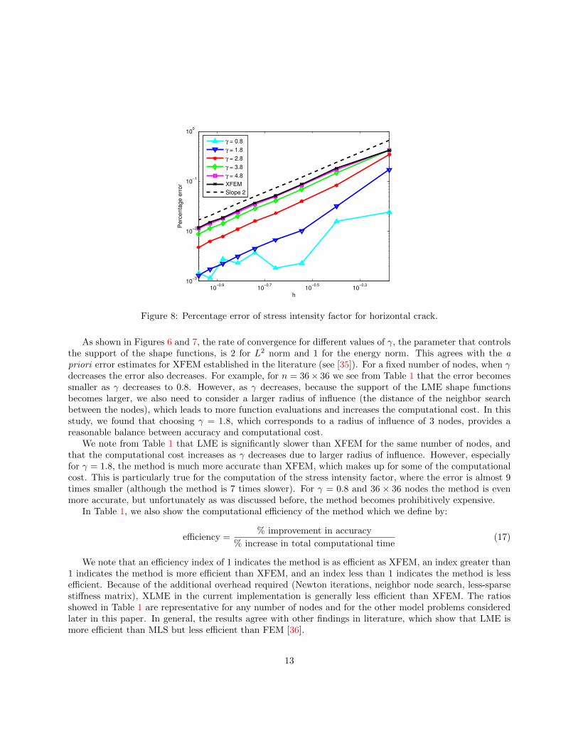
Approximation errors in L2 norm and energy norm are illustrated in Figures 6 and 7 for different values ofγ. Figure 8 shows the percentage error for stress intensity factor (SIFs). It is obvious from these figures thatin this case there is an optimal value for the parameter γ of around 1.8 for which accuracy is maximized. Forvery low values of γ, convergence is degraded. This is due to numerical integration. With a higher numberof Gauss points and γ = 0.8, the optimal rate of convergence for a plane elasticity problem was recoveredin [5]. But in that case, the method is very expensive. The LME results converge to the standard XFEMresults as γ increases.

12

10−0.9

10−0.7

10−0.5

10−0.3

10−3

10−2

10−1

100

h

Pe

rce

nta

ge

err

or

γ = 0.8

γ = 1.8

γ = 2.8

γ = 3.8

γ = 4.8

XFEM

Slope 2

Figure 8: Percentage error of stress intensity factor for horizontal crack.

As shown in Figures 6 and 7, the rate of convergence for different values of γ, the parameter that controlsthe support of the shape functions, is 2 for L2 norm and 1 for the energy norm. This agrees with the apriori error estimates for XFEM established in the literature (see [35]). For a fixed number of nodes, when γdecreases the error also decreases. For example, for n = 36× 36 we see from Table 1 that the error becomessmaller as γ decreases to 0.8. However, as γ decreases, because the support of the LME shape functionsbecomes larger, we also need to consider a larger radius of influence (the distance of the neighbor searchbetween the nodes), which leads to more function evaluations and increases the computational cost. In thisstudy, we found that choosing γ = 1.8, which corresponds to a radius of influence of 3 nodes, provides areasonable balance between accuracy and computational cost.

We note from Table 1 that LME is significantly slower than XFEM for the same number of nodes, andthat the computational cost increases as γ decreases due to larger radius of influence. However, especiallyfor γ = 1.8, the method is much more accurate than XFEM, which makes up for some of the computationalcost. This is particularly true for the computation of the stress intensity factor, where the error is almost 9times smaller (although the method is 7 times slower). For γ = 0.8 and 36 × 36 nodes the method is evenmore accurate, but unfortunately as was discussed before, the method becomes prohibitively expensive.

In Table 1, we also show the computational efficiency of the method which we define by:

efficiency =% improvement in accuracy

% increase in total computational time(17)

We note that an efficiency index of 1 indicates the method is as efficient as XFEM, an index greater than1 indicates the method is more efficient than XFEM, and an index less than 1 indicates the method is lessefficient. Because of the additional overhead required (Newton iterations, neighbor node search, less-sparsestiffness matrix), XLME in the current implementation is generally less efficient than XFEM. The ratiosshowed in Table 1 are representative for any number of nodes and for the other model problems consideredlater in this paper. In general, the results agree with other findings in literature, which show that LME ismore efficient than MLS but less efficient than FEM [36].

13

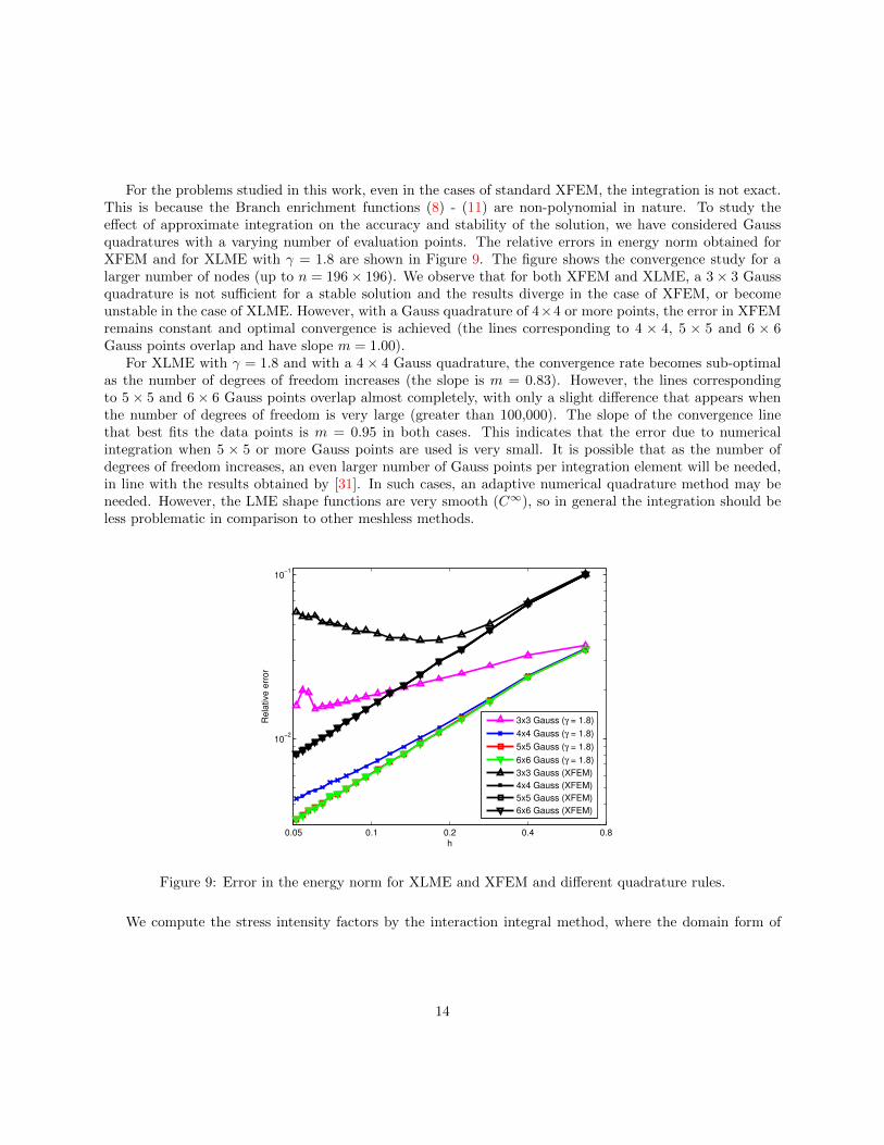
For the problems studied in this work, even in the cases of standard XFEM, the integration is not exact.This is because the Branch enrichment functions (8) - (11) are non-polynomial in nature. To study theeffect of approximate integration on the accuracy and stability of the solution, we have considered Gaussquadratures with a varying number of evaluation points. The relative errors in energy norm obtained forXFEM and for XLME with γ = 1.8 are shown in Figure 9. The figure shows the convergence study for alarger number of nodes (up to n = 196× 196). We observe that for both XFEM and XLME, a 3× 3 Gaussquadrature is not sufficient for a stable solution and the results diverge in the case of XFEM, or becomeunstable in the case of XLME. However, with a Gauss quadrature of 4×4 or more points, the error in XFEMremains constant and optimal convergence is achieved (the lines corresponding to 4 × 4, 5 × 5 and 6 × 6Gauss points overlap and have slope m = 1.00).

For XLME with γ = 1.8 and with a 4× 4 Gauss quadrature, the convergence rate becomes sub-optimalas the number of degrees of freedom increases (the slope is m = 0.83). However, the lines correspondingto 5× 5 and 6× 6 Gauss points overlap almost completely, with only a slight difference that appears whenthe number of degrees of freedom is very large (greater than 100,000). The slope of the convergence linethat best fits the data points is m = 0.95 in both cases. This indicates that the error due to numericalintegration when 5 × 5 or more Gauss points are used is very small. It is possible that as the number ofdegrees of freedom increases, an even larger number of Gauss points per integration element will be needed,in line with the results obtained by [31]. In such cases, an adaptive numerical quadrature method may beneeded. However, the LME shape functions are very smooth (C∞), so in general the integration should beless problematic in comparison to other meshless methods.

0.05 0.1 0.2 0.4 0.8

10−2

10−1

h

Re

lative

err

or

3x3 Gauss (γ = 1.8)

4x4 Gauss (γ = 1.8)

5x5 Gauss (γ = 1.8)

6x6 Gauss (γ = 1.8)

3x3 Gauss (XFEM)

4x4 Gauss (XFEM)

5x5 Gauss (XFEM)

6x6 Gauss (XFEM)

Figure 9: Error in the energy norm for XLME and XFEM and different quadrature rules.

We compute the stress intensity factors by the interaction integral method, where the domain form of

14

the interaction integral is given by [37]

I(1,2) =

∫A

[σ

(1)ij

∂u2i

∂x1− σ(2)

ij

∂u1i

∂x1−W (1,2)δ1j

]∂q

∂xjdA

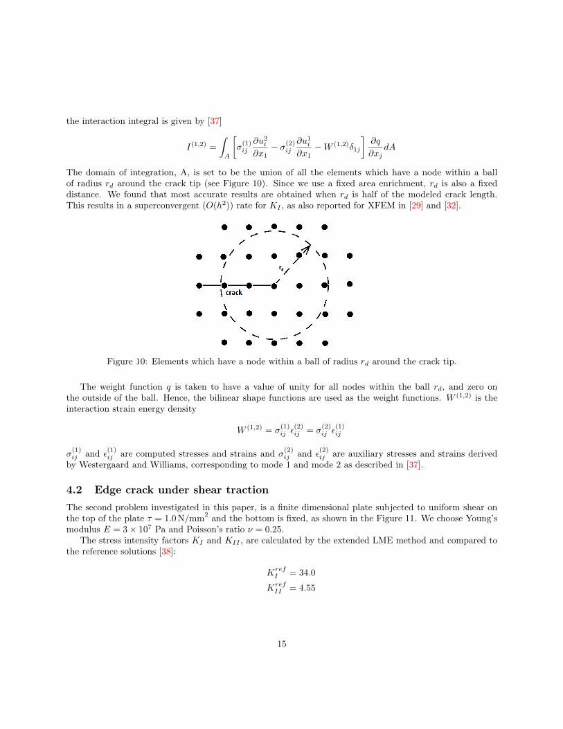
The domain of integration, A, is set to be the union of all the elements which have a node within a ballof radius rd around the crack tip (see Figure 10). Since we use a fixed area enrichment, rd is also a fixeddistance. We found that most accurate results are obtained when rd is half of the modeled crack length.This results in a superconvergent (O(h2)) rate for KI , as also reported for XFEM in [29] and [32].

Figure 10: Elements which have a node within a ball of radius rd around the crack tip.

The weight function q is taken to have a value of unity for all nodes within the ball rd, and zero onthe outside of the ball. Hence, the bilinear shape functions are used as the weight functions. W (1,2) is theinteraction strain energy density

W (1,2) = σ(1)ij ε

(2)ij = σ

(2)ij ε

(1)ij

σ(1)ij and ε

(1)ij are computed stresses and strains and σ

(2)ij and ε

(2)ij are auxiliary stresses and strains derived

by Westergaard and Williams, corresponding to mode 1 and mode 2 as described in [37].

4.2 Edge crack under shear traction

The second problem investigated in this paper, is a finite dimensional plate subjected to uniform shear onthe top of the plate τ = 1.0 N/mm

2and the bottom is fixed, as shown in the Figure 11. We choose Young’s

modulus E = 3× 107 Pa and Poisson’s ratio ν = 0.25.The stress intensity factors KI and KII , are calculated by the extended LME method and compared to

the reference solutions [38]:

KrefI = 34.0

KrefII = 4.55

15

Figure 11: Edge-cracked plate under shear stress.

We note that these values were calculated using a boundary collocation method and are given with anaccuracy of 3 significant digits. The SIFs KI and KII calculated by the extended LME method on a finemesh converge to the following values (accurate to 4 significant digits):

K0I = 34.04

K0II = 4.537

We note that there is a very good agreement between the reference solution and our computed solution.To study the convergence of the method we calculated the percentage error between the computed SIFs atvarious levels of refinement and K0

I and K0II .

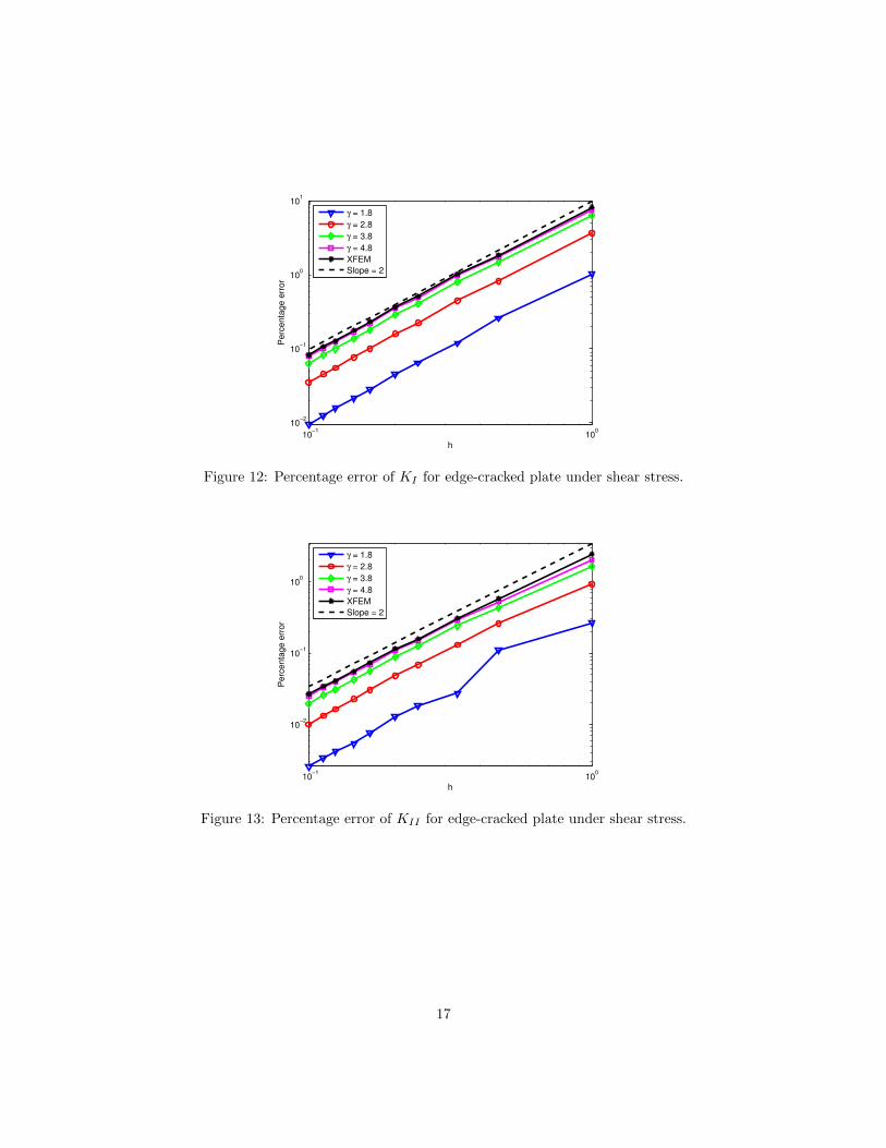
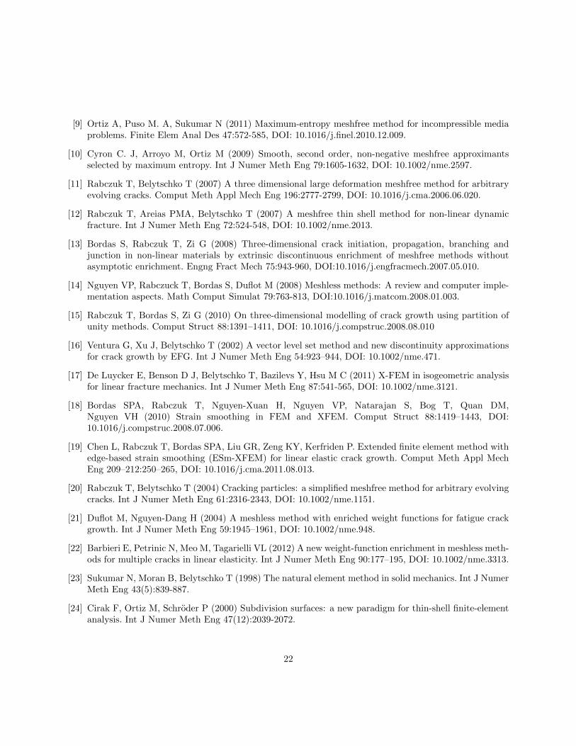
Figures 12 and 13 illustrate the percentage error for KI and KII . As evident from these figures, thesmallest error for this problem is obtained by γ = 1.8 and γ = 2.8. We note that for these values of γ theerror becomes less than 0.01%, which is equal to K0

I and K0II up to the given significant digits. For values

of γ that are lower than 1.8, computing the SIF accurately becomes expensive due to the large support ofthe shape functions. Therefore, we will not consider the case γ = 0.8 in the following examples.

16

10−1

100

10−2

10−1

100

101

h

Perc

enta

ge e

rror

γ = 1.8

γ = 2.8

γ = 3.8

γ = 4.8

XFEM

Slope = 2

Figure 12: Percentage error of KI for edge-cracked plate under shear stress.

10−1

100

10−2

10−1

100

h

Perc

enta

ge e

rror

γ = 1.8

γ = 2.8

γ = 3.8

γ = 4.8

XFEM

Slope = 2

Figure 13: Percentage error of KII for edge-cracked plate under shear stress.

17

4.3 Slanted crack in an infinite plate

Consider an infinite plate containing an angled crack as shown in Figure 14a. This problem is a mixed modeI-II problem. The analytical near-tip field solution for this problem in polar coordinates is given in [39]

σxx(r, θ) =KI√2πr

cosθ

2

(1− sin

θ

2sin

3θ

2

)− KII√

2πrsin

θ

2

(2 + cos

θ

2cos

3θ

2

)σyy(r, θ) =

KI√2πr

cosθ

2

(1 + sin

θ

2sin

3θ

2

)+

KII√2πr

sinθ

2cos

θ

2cos

3θ

2

σxy(r, θ) =KI√2πr

sinθ

2cos

θ

2cos

3θ

2

+KII√2πr

cosθ

2

(1− sin

θ

2sin

3θ

2

)

ux(r, θ) =KI

2µ

√r

2πcos

θ

2

(κ− 1 + 2 sin2 θ

2

)+KII

2µ

√r

2πsin

θ

2

(κ+ 1 + 2 cos2 θ

2

)uy(r, θ) =

KI

2µ

√r

2πsin

θ

2

(κ+ 1− 2 cos2 θ

2

)− KII

2µ

√r

2πcos

θ

2

(κ− 1− 2 sin2 θ

2

)Here µ is the shear modulus, κ = 3− 4υ for plane strain. The angle θ and the distance r from the crack tipare indicated in Figure 14b.

18

Figure 14: a) Slanted crack in an infinite plate where the principal stress is not perpendicular to the crack.b) An infinite plate rotated with respect to the crack’s angle.

We redefine the x-coordinate axis to coincide with the crack orientation [40], see Figure 14b. The appliedstress is decomposed into normal and shear components. The stress normal to the crack, σyy, produces puremode I loading, while σxy applies mode II loading to the crack. The stress intensity factors for the plate,can be computed by the relationship between σyy and σxy relative to σ and α through Mohr’s circle [41]

KI = σyy√πa = σ cos2 α

√πa

KII = σxy√πa = σ sinα cosα

√πa

In this problem, we again modeled a square region around the crack tip, the gray square in Figure 14b, andchose different values for crack’s angle. The same tendency as for the 1st example is observed for this mixedmode problem. Again, γ = 1.8 gives the most accurate results and this method has a convergence rate ofapproximately 2.

Table 2: Error and the average running time when the number of nodes is 36 × 36, the number of Gausspoints is 16, α = 15, 30 and radius of influence is 2 for γ = 4.8 and γ = 3.8, 3 for γ = 2.8 and γ = 1.8

γ Relative Relative Relative Relative Average totalerror error error error runningof KI , of KII , of KI , of KII , time (seconds)α = 15 α = 15 α = 30 α = 30

XFEM 0.088212 0.014660 0.088209 0.014663 15.74.8 0.084748 0.013936 0.084753 0.013924 49.03.8 0.070224 0.011169 0.070251 0.011112 46.72.8 0.039802 0.005500 0.039819 0.005465 101.41.8 0.010153 0.002018 0.010146 0.002010 99.9

As shown in Table 2 when γ decreases to the optimal value, in this case γ = 1.8, the error decreases,however the computational cost increases due to a larger radius of influence of the shape functions. Nev-

19

ertheless, we note that the error is much smaller (almost an order of magnitude) between γ = 4.8, whichis virtually the same as standard XFEM, and γ = 1.8. We note that there is only a very small differencebetween the α = 15 and α = 30. This can be explained by the fact that the discretization is identical, theonly difference being the size of the forces applied to the boundaries, as can been seen from Figure 14. Thelog-log plots indicating the convergence rates of KI and KII with α = 30 are shown in Figures 15 and 16.We also computed the errors for KI and KII for angles α = 45, 60, 75 with similar results.

10−0.9

10−0.8

10−0.7

10−0.6

10−3

10−2

10−1

100

h

Perc

enta

ge e

rror

γ = 1.8

γ = 2.8

γ = 3.8

γ = 4.8

XFEM

Slope 2

Figure 15: Percentage error of KI for slanted crack in an infinite plate with α = 30.

10−0.9

10−0.8

10−0.7

10−0.6

10−5

10−4

10−3

10−2

10−1

h

Perc

enta

ge e

rror

γ = 1.8

γ = 2.8

γ = 3.8

γ = 4.8

XFEM

Slope 2

Figure 16: Percentage error of KII for slanted crack in an infinite plate with α = 30.

20

5 Conclusions

We have developed a local maximum entropy approximation scheme for fracture using enrichment functions.The LME shape functions are non-negative which improves stability, and they possess a weak Kroneckerdelta property which makes it easy to impose the boundary conditions. With a fixed area (geometric)enrichment, optimal convergence is obtained. The LME basis functions are in general not polynomialsbut rather particle-based smooth functions, whose support is dictated by a non-dimensional parameter γ.When γ decreases, the LME shape functions have better approximation properties compared to standardFEM shape functions, but the size of their support increases. Hence, accurate numerical integration usingstandard Gauss quadrature requires a greater number of function evaluations. We conclude that there is anoptimal value of γ of around 1.8 that maximizes the accuracy in relation to computational cost.

For computation of stress intensity factors, this method is competitive in terms of costs compared toXFEM. Very likely, it is possible to improve the computational efficiency further. In particular, we plan toinvestigate the development of an efficient integration scheme, goal-oriented adaptivity for the parameterγ and the enrichment radius, as well as methods to improve the condition number of the stiffness matrix.The proposed approximation also shows a lot of potential for other problems which will be examined in thefuture, such as crack growth and fracture in thin shell bodies.

Acknowledgements

The first two authors would like to thank the Free State of Thuringia and Bauhaus Research School forfinancial support during the duration of this project. We would also like to thank the anonymous reviewersfor their helpful comments and suggestions.

References

[1] Sukumar N (2004) Construction of polygonal interpolants: a maximum entropy approach. Int J NumerMeth Eng 61(12):2159-2181, DOI: 10.1002/nme.1193.

[2] Shannon C. E (1948) A mathematical theory of communication. Bell Labs Tech J 27:379–423.

[3] Jaynes E. T (1957) Information theory and statistical mechanics. Phys Rev 106(4):620–630, DOI:10.1103/PhysRev.106.620.

[4] Jaynes E. T (1957) Information theory and statistical mechanics II. Phys Rev 108(2):171–190, DOI:10.1103/PhysRev.103.171.

[5] Arroyo M, Ortiz M (2006) Local maximum-entropy approximation schemes: a seamless bridge betweenfinite elements and meshfree methods. Int J Numer Meth Eng 65:2167-2202, DOI: 10.1002/nme.1534.

[6] Shepard D (1968) A two dimensional interpolation function for irregularly spaced data. Proc. 23rd Nat.Conf. ACM pages 517–523, ACM. DOI: 10.1145/800186.810616

[7] Millan D, Rosolen A, Arroyo M (2011) Thin shell analysis from scattered points with maximum-entropyapproximants. Int J Numer Meth Eng 85:723-751, DOI: 10.1002/nme.2992.

[8] Ortiz A, Puso M. A, Sukumar N (2010) Maximum-entropy meshfree method for compressible and near-incompressible elasticity. Comput Meth Appl Mech Eng 199:1859-1871, DOI: 10.1016/j.cma.2010.02.013.

21

[9] Ortiz A, Puso M. A, Sukumar N (2011) Maximum-entropy meshfree method for incompressible mediaproblems. Finite Elem Anal Des 47:572-585, DOI: 10.1016/j.finel.2010.12.009.

[10] Cyron C. J, Arroyo M, Ortiz M (2009) Smooth, second order, non-negative meshfree approximantsselected by maximum entropy. Int J Numer Meth Eng 79:1605-1632, DOI: 10.1002/nme.2597.

[11] Rabczuk T, Belytschko T (2007) A three dimensional large deformation meshfree method for arbitraryevolving cracks. Comput Meth Appl Mech Eng 196:2777-2799, DOI: 10.1016/j.cma.2006.06.020.

[12] Rabczuk T, Areias PMA, Belytschko T (2007) A meshfree thin shell method for non-linear dynamicfracture. Int J Numer Meth Eng 72:524-548, DOI: 10.1002/nme.2013.

[13] Bordas S, Rabczuk T, Zi G (2008) Three-dimensional crack initiation, propagation, branching andjunction in non-linear materials by extrinsic discontinuous enrichment of meshfree methods withoutasymptotic enrichment. Engng Fract Mech 75:943-960, DOI:10.1016/j.engfracmech.2007.05.010.

[14] Nguyen VP, Rabczuck T, Bordas S, Duflot M (2008) Meshless methods: A review and computer imple-mentation aspects. Math Comput Simulat 79:763-813, DOI:10.1016/j.matcom.2008.01.003.

[15] Rabczuk T, Bordas S, Zi G (2010) On three-dimensional modelling of crack growth using partition ofunity methods. Comput Struct 88:1391–1411, DOI: 10.1016/j.compstruc.2008.08.010

[16] Ventura G, Xu J, Belytschko T (2002) A vector level set method and new discontinuity approximationsfor crack growth by EFG. Int J Numer Meth Eng 54:923–944, DOI: 10.1002/nme.471.

[17] De Luycker E, Benson D J, Belytschko T, Bazilevs Y, Hsu M C (2011) X-FEM in isogeometric analysisfor linear fracture mechanics. Int J Numer Meth Eng 87:541-565, DOI: 10.1002/nme.3121.

[18] Bordas SPA, Rabczuk T, Nguyen-Xuan H, Nguyen VP, Natarajan S, Bog T, Quan DM,Nguyen VH (2010) Strain smoothing in FEM and XFEM. Comput Struct 88:1419–1443, DOI:10.1016/j.compstruc.2008.07.006.

[19] Chen L, Rabczuk T, Bordas SPA, Liu GR, Zeng KY, Kerfriden P. Extended finite element method withedge-based strain smoothing (ESm-XFEM) for linear elastic crack growth. Comput Meth Appl MechEng 209–212:250–265, DOI: 10.1016/j.cma.2011.08.013.

[20] Rabczuk T, Belytschko T (2004) Cracking particles: a simplified meshfree method for arbitrary evolvingcracks. Int J Numer Meth Eng 61:2316-2343, DOI: 10.1002/nme.1151.

[21] Duflot M, Nguyen-Dang H (2004) A meshless method with enriched weight functions for fatigue crackgrowth. Int J Numer Meth Eng 59:1945–1961, DOI: 10.1002/nme.948.

[22] Barbieri E, Petrinic N, Meo M, Tagarielli VL (2012) A new weight-function enrichment in meshless meth-ods for multiple cracks in linear elasticity. Int J Numer Meth Eng 90:177–195, DOI: 10.1002/nme.3313.

[23] Sukumar N, Moran B, Belytschko T (1998) The natural element method in solid mechanics. Int J NumerMeth Eng 43(5):839-887.

[24] Cirak F, Ortiz M, Schroder P (2000) Subdivision surfaces: a new paradigm for thin-shell finite-elementanalysis. Int J Numer Meth Eng 47(12):2039-2072.

22

[25] Hughes T, Cottrell J, Bazilevs Y (2005) Isogeometric analysis: CAD, finite elements, NURBS,exact geometry and mesh refinement. Comput Meth Appl Mech Eng 194:4135-4195, DOI:10.1016/j.cma.2004.10.008.

[26] Rajan V (1994) Optimality of the Delaunay triangulation in Rd. Discrete Comput Geom 12(2):189-202,DOI: 10.1007/BF02574375.

[27] Rabczuk T, Wall WA (2007) EXtended finite element and meshfree methods. Technical University ofMunich, Germany.

[28] Stazi F L, Budyn E, Chessa J, Belytschko T (2003) An extended finite element method with higher-orderelements for curved cracks. Comput Mech 31(1-2):38-48, DOI: 10.1007/s00466-002-0391-2.

[29] Laborde P, Pommier J, Renard Y, Salaun M (2005) High-order extended finite element method forcracked domains. Int J Numer Meth Eng 64(12):354-381, DOI: 10.1002/nme.1370.

[30] Natarajan S, Mahapatra DR, Bordas SPA (2010) Integrating strong and weak discontinuities withoutintegration subcells and example applications in an XFEM/GFEM framework. Int J Numer Meth Eng83:269-294, DOI: 10.1002/nme.2798.

[31] Babuka I, Banerjee U, Osborn JE, Zhang Q (2009) Effect of numerical integration on meshless methodsComput Meth Appl Mech Eng 198 2886-2897, DOI: 10.1016/j.cma.2009.04.008

[32] Bechet E, Minnebo H, Moes N, Burgardt B (2005) Improved implementation and robustness study of theX-FEM for stress analysis around cracks. Int J Numer Meth Eng 64:1033-1056, DOI: 10.1002/nme.1386.

[33] Menk A, Bordas SPA (2011) A robust preconditioning technique for the extended finite element method.Int J Numer Meth Eng 85:1609-1632, DOI: 10.1002/nme.3032.

[34] Babuska I, Banerjee U (2011) Stable generalized finite element method (SGFEM). Comput Meth ApplMech Eng 201-204:91-111, DOI: 10.1016/j.cma.2011.09.012.

[35] Nicaise S, Renard Y, Chahine E (2011) Optimal convergence analysis for the extended finite elementmethod. Int J Numer Meth Engng 86:528548

[36] Quak W, van den Boogaard AH, Gonzalez D, Cueto E (2011) A comparative study on the performanceof meshless approximations and their integration. Comput Mech 48(2):121-137, DOI: 10.1007/s00466-011-0577-6.

[37] Moes N, Dolbow J, Belytscho T (1999) A finite element method for crack growth without remeshing.Int J Numer Meth Eng 46:131-150.

[38] Yau J, Wang S, Corten H (1980) A mixed-mode crack analysis of isotropic solids using conservationlaws of elasticity. J Appl Mech 47:335-341, DOI: 10.1115/1.3153665.

[39] Zehnder A (2010) Fracture mechanics. Cornell University, Lecture Notes.

[40] Rabczuk T, Si G (2006) A meshfree method based on the local partition of unity for cohesive cracks.Comput Mech 39(6):743-760, DOI: 10.1007/s00466-006-0067-4.

[41] Anderson TL (1995) Fracture mechanics, fundamentals and applications. Second edition; Texas A&MUniversity.

23