Astronomy & Astrophysics manuscript no. paper c©ESO 2013June 24, 2013

COSMOGRAIL: the COSmological MOnitoring ofGRAvItational Lenses?,??

XIV. Time delay of the doubly lensed quasar SDSS J1001+5027

S. Rathna Kumar1, M. Tewes2, C. S. Stalin1, F. Courbin2, I. Asfandiyarov3, G. Meylan2, E. Eulaers4, T. P. Prabhu1,P. Magain4, H. Van Winckel5, and Sh. Ehgamberdiev3

1 Indian Institute of Astrophysics, II Block, Koramangala, Bangalore 560 034, India, e-mail: rathna@iiap.res.in2 Laboratoire d’astrophysique, Ecole Polytechnique Fédérale de Lausanne (EPFL), Observatoire de Sauverny, 1290 Versoix, Switzer-

land3 Ulugh Beg Astronomical Institute, Uzbek Academy of Sciences, Astronomicheskaya 33, Tashkent, 100052, Uzbekistan4 Institut d’Astrophysique et de Géophysique, Université de Liège, Allée du 6 Août, 17, 4000 Sart Tilman, Liège 1, Belgium5 Instituut voor Sterrenkunde, Katholieke Universiteit Leuven, Celestijnenlaan 200B, 3001 Heverlee, Belgium

Received / Accepted

ABSTRACT

This paper presents optical R-band light curves and the time delay of the doubly imaged gravitationally lensed quasarSDSS J1001+5027 at a redshift of 1.838. We have observed this target for more than six years, between March 2005 and July 2011,using the 1.2-m Mercator Telescope, the 1.5-m telescope of the Maidanak Observatory and the 2-m Himalayan Chandra Telescope.Our resulting light curves are composed of 443 independent epochs, and show strong intrinsic quasar variability, with an amplitude ofthe order of 0.2 magnitudes. From this data, we measure the time delay using five different methods, all relying on distinct approaches.One of these techniques is a new development presented in this paper. All our time-delay measurements are perfectly compatible. Bycombining them, we conclude that image A is leading B by 119.3 ± 3.3 days (1σ, 2.8%), including systematic errors. It has beenshown recently that such accurate time-delay measurements offer a highly complementary probe of dark energy and spatial curvature,as they independently constrain the Hubble constant. The next mandatory step towards using SDSS J1001+5027 in this context willbe the measurement of the redshift of the lensing galaxy, in combination with deep HST imaging.

Key words. gravitational lensing: strong – cosmological parameters – quasar: individual (SDSS J1001+5027)

1. Introduction

In the current cosmological paradigm, only a handful of para-meters seem necessary to describe the Universe on its largestscales and its evolution with time. Testing this cosmologicalmodel requires a range of experiments, characterized by differentsensitivities to these parameters. These experiments, or cosmo-logical probes, are all affected by statistical and systematic errorsand none of them, on its own, can constrain uniquely the cosmo-logical models. This is due to the degeneracies inherent to eachspecific probe, implying that the probes become truly effectivein constraining cosmology only when combined together.

The latest cosmology results by the Planck consortium beau-tifully illustrate this (Planck Collaboration 2013). In particu-lar, the constraints obtained by Planck on the Hubble parame-ter H0, on the curvature, Ωk, and on the dark energy equation ofstate parameter w mostly rely on the combination of the Bary-

? Based on observations made with the 2.0-m Himalayan ChandraTelescope (Hanle, India), the 1.5-m AZT-22 telescope (Maidanak Ob-servatory, Uzbekistan), and the 1.2-m Mercator Telescope. Mercator isoperated on the island of La Palma by the Flemish Community, at theSpanish Observatorio del Roque de los Muchachos of the Instituto deAstrofísica de Canarias.?? Light curves will be available at the CDS via anonymous ftp tocdsarc.u-strasbg.fr (130.79.128.5) or via http://cdsarc.u-strasbg.fr/viz-bin/qcat?J/A+A/???, and on http://www.cosmograil.org.

onic Acoustic Oscillations measurements (BAO) with the Cos-mic Microwave Background (CMB) observations.

Strong gravitational lensing offers a valuable yet cheap com-plement to independently constrain some of the cosmologicalparameters, through the measurement of the so-called "time de-lays" in quasars strongly lensed by a foreground galaxy (Refsdal1964). The principle of the method is the following. The traveltimes of photons along the distinct optical paths forming themultiple images are not identical. These travel time differences,namely the time delays, depend on the geometrical differencesbetween the optical paths (which contain the cosmological in-formation) and on the potential well of the lensing galaxy(ies).In practice, time delays can be measured from photometric lightcurves of the multiple images of lensed quasar: if the quasarshows photometric variations, these are seen in the individuallight curves at epochs separated by the time delay.

A precise and accurate measurement of such a time delay,in combination with a well-constrained model for the lensinggalaxy, can therefore be used to extract cosmological informa-tion. The excellent performance and strong competitiveness ofthis time-delay method has recently been quantified by Suyuet al. (2013a) (see also Schneider & Sluse 2013; Suyu et al.2013b), Linder (2011), and summarized in Treu et al. (2013).

So far, only a few quasar time delays have been measuredconvincingly, from long and well sampled light curves. The

Article number, page 1 of 7

arX

iv:1

306.

5105

v1 [

astr

o-ph

.CO

] 2

1 Ju

n 20

13

A&A proofs: manuscript no. paper

1.0 1.5 2.0 2.5 3.0FWHM [arcsec]

1.05 1.10 1.15 1.20 1.25 1.30

ε=a/b

MercatorHCTMaidanak

Fig. 1. Distribution of the average observed FWHM and elonga-tion ε of field stars in the images used to build the light curves ofSDSS J1001+5027.

international COSMOGRAIL1 (COSmological MOnitoring ofGRAvItational Lenses) collaboration is changing this situationby measuring accurate time delays for a large number of gravita-tionally lensed quasars. The goal of COSMOGRAIL is to reachan accuracy of less than 3%, including systematics, for most ofits targets.

In this paper, we present the time-delay measurement forthe two-image gravitationally lensed quasar SDSS J1001+5027(α2000 = 10:01:28.61, δ2000 = +50:27:56.90), at z = 1.838 (Oguriet al. 2005). The image separation of ∆θ = 2.86′′(Oguri et al.2005) and the high declination of the target makes it a relativelyeasy prey for medium size northern telescopes and average see-ing conditions. The redshift of the lensing galaxy has not beenmeasured spectroscopically but Oguri et al. (2005) measure col-ors suggestive of an elliptical galaxy at a redshift in the range0.2 < z < 0.5.

Our paper is structured as follows. Section 2 describes ourmonitoring, the data reduction, and the resulting light curves.In Section 3 we present a new time-delay point estimator. Weadd this technique to a pool of four other existing algorithms, tomeasure the time delay in Section 4. Finally, we summarize ourresults and conclude in Section 5.

2. Observations, data reduction, and light curves

2.1. Observations

We monitored SDSS J1001+5027 in the R-band for more than 6years, from March 2005 to July 2011, with three different tele-scopes: the 1.2-m Mercator Telescope located at the Roque delos Muchachos Observatory on La Palma (Spain), the 1.5-m tele-scope of the Maidanak Observatory in Pamir Alai (Uzbekistan),and the 2-m Himalayan Chandra Telescope (HCT) located at theIndian Astronomical Observatory in Hanle (India). Table 1 de-tails our monitoring observations. In total we obtained photo-metric measurements for 443 independent epochs, with a meansampling interval below 4 days. Each epoch consists of at least 3,but mostly 4 or more, dithered exposures. Figure 1 summarizesthe image quality of our data. The COSMOGRAIL collaborationhas now ceased the monitoring of this target, to focus on othersystems.

2.2. Deconvolution photometry

The image reduction and photometry closely follows the proce-dure described in Tewes et al. (2013b). We perform the flat-field

1 http://www.cosmograil.org/

correction and bias subtraction for each exposure using customsoftware pipelines, which address the particularities of the dif-ferent telescopes and instruments.

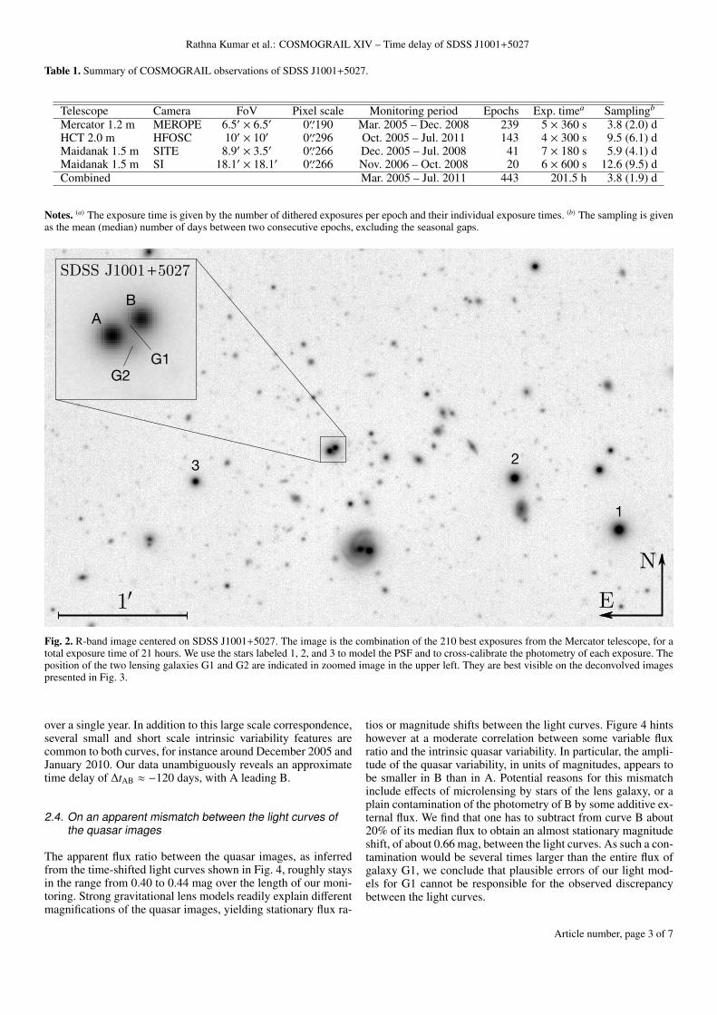
Figure 2 shows part of the field around SDSS J1001+5027,as obtained by stacking the best monitoring exposures from theMercator telescope to reach an integrated exposure time of 21hours. The relative flux measurements of the quasar images andreference stars, for each individual epoch, are obtained thoughour COSMOGRAIL photometry pipeline, which is based onthe simultaneous MCS deconvolution algorithm (Magain et al.1998). The stars labeled 1, 2, and 3 in Fig. 2 are used to char-acterize the Point Spread Function (PSF) and relative magnitudezero-point of each exposure.

The 2 quasar images A and B of SDSS J1001+5027 are sep-arated by 2.86′′, which is significantly larger than the typicalseparation in strongly lensed quasars. In principle, this makesSDSS J1001+5027 a relatively easy target to monitor, as thequasar images are only slightly blended in most of our images.However, image B lies close to the primary lensing galaxy G1.Minimizing the additive contamination by G1 to the flux mea-surements of B therefore requires a model for the light distribu-tion of G1. In Fig. 3, we show two different ways of modelingthese galaxies. Our standard approach, shown in the bottom pan-els, consists in representing all extended objects, such as the lensgalaxies, by a regularized pixel grid. The values of these pix-els get iteratively updated during the deconvolution photometryprocedure. Due to obvious degeneracies, this approach may failwhen a relatively small extended object (lens galaxy) is stronglyblended with a bright point source (quasar), leading to unphysi-cal light distributions. To explore the sensitivity of our results tosuch a possible bias, we have adopted an alternative approach,by representing G1 and G2 by two simply parametrized ellipticalSersic profiles, as shown in the top row of Fig. 3. For both cases,the residuals from single exposures are convincingly homoge-neous. Only when averaging the residuals of many exposures todecrease the noise, it can be seen that the simply parametrizedmodels yield a less good overall fit to the data, since they cannotrepresent further background sources nor compensate for smallsystematic errors in the shape of the PSF.

We find that the difference between these approaches interms of the resulting quasar flux photometry is very marginal,and insignificant regarding the measurement of the time delay.In all the following we will use the quasar photometry obtainedusing the simply parametrized model (top row of Fig. 3), whichis likely to be closer to reality than our pixelized model, in theimmediate surroundings of image B.

2.3. Light curves

Following Tewes et al. (2013b), we empirically correct for smallmagnitude and flux shifts between the light curve contributionsfrom different telescopes/cameras, to obtain minimal dispersionin each of the combined light curves. In the present case wechoose the photometry from the Mercator telescope as a refer-ence, and we optimize, for the data from the Maidanak and HCTtelescopes, a common magnitude shift and individual flux shiftsfor A and B.

Figure 4 shows the combined 6.5-season long light curves,from which we measure a time delay of ∆tAB = −119.3 days(see Section 4). In this figure, the light curve B has been shiftedby this time delay, to highlight the correspondence and temporaloverlap of the data. We observe strong “intrinsic” quasar vari-ability, common to the images A and B. In the period 2006 to2007, the variability in image A is as large as 0.25 magnitudes

Article number, page 2 of 7

Rathna Kumar et al.: COSMOGRAIL XIV – Time delay of SDSS J1001+5027

Table 1. Summary of COSMOGRAIL observations of SDSS J1001+5027.

Telescope Camera FoV Pixel scale Monitoring period Epochs Exp. timea Samplingb

Mercator 1.2 m MEROPE 6.5′ × 6.5′ 0′′.190 Mar. 2005 – Dec. 2008 239 5 × 360 s 3.8 (2.0) dHCT 2.0 m HFOSC 10′ × 10′ 0′′.296 Oct. 2005 – Jul. 2011 143 4 × 300 s 9.5 (6.1) dMaidanak 1.5 m SITE 8.9′ × 3.5′ 0′′.266 Dec. 2005 – Jul. 2008 41 7 × 180 s 5.9 (4.1) dMaidanak 1.5 m SI 18.1′ × 18.1′ 0′′.266 Nov. 2006 – Oct. 2008 20 6 × 600 s 12.6 (9.5) dCombined Mar. 2005 – Jul. 2011 443 201.5 h 3.8 (1.9) d

Notes. (a) The exposure time is given by the number of dithered exposures per epoch and their individual exposure times. (b) The sampling is givenas the mean (median) number of days between two consecutive epochs, excluding the seasonal gaps.

E

N

1

23

1'

AB

SDSS J1001 5027 +

G2G1

Fig. 2. R-band image centered on SDSS J1001+5027. The image is the combination of the 210 best exposures from the Mercator telescope, for atotal exposure time of 21 hours. We use the stars labeled 1, 2, and 3 to model the PSF and to cross-calibrate the photometry of each exposure. Theposition of the two lensing galaxies G1 and G2 are indicated in zoomed image in the upper left. They are best visible on the deconvolved imagespresented in Fig. 3.

over a single year. In addition to this large scale correspondence,several small and short scale intrinsic variability features arecommon to both curves, for instance around December 2005 andJanuary 2010. Our data unambiguously reveals an approximatetime delay of ∆tAB ≈ −120 days, with A leading B.

2.4. On an apparent mismatch between the light curves ofthe quasar images

The apparent flux ratio between the quasar images, as inferredfrom the time-shifted light curves shown in Fig. 4, roughly staysin the range from 0.40 to 0.44 mag over the length of our moni-toring. Strong gravitational lens models readily explain differentmagnifications of the quasar images, yielding stationary flux ra-

tios or magnitude shifts between the light curves. Figure 4 hintshowever at a moderate correlation between some variable fluxratio and the intrinsic quasar variability. In particular, the ampli-tude of the quasar variability, in units of magnitudes, appears tobe smaller in B than in A. Potential reasons for this mismatchinclude effects of microlensing by stars of the lens galaxy, or aplain contamination of the photometry of B by some additive ex-ternal flux. We find that one has to subtract from curve B about20% of its median flux to obtain an almost stationary magnitudeshift, of about 0.66 mag, between the light curves. As such a con-tamination would be several times larger than the entire flux ofgalaxy G1, we conclude that plausible errors of our light mod-els for G1 cannot be responsible for the observed discrepancybetween the light curves.

Article number, page 3 of 7

A&A proofs: manuscript no. paper

3''

Single exposure

Parametric model

Pixelized model

Residuals

Residuals

Average residuals

Average residuals

Fig. 3. Illustration of the two ways of modeling the light-distribution for extended objects, during the deconvolution process. On the left is shown asingle 360 second exposure of SDSS J1001+5027 obtained with the Mercator telescope in typical atmospheric conditions. The other panels showthe parametric (top row) and pixelized light models (bottom row) for the lens galaxies, as described in the text. The residual image for the singleexposure is also shown in each case, as well as the average residuals over the 120 best exposures. The residual maps are normalized by the shotnoise amplitude. The dark areas indicate excess flux in the data with respect to the model. Gray scales are linear.

53500 54000 54500 55000 55500HJD - 2400000.5 [day]

0.0

0.1

0.2

0.3

0.4

0.5

Magnit

ude (

rela

tive)

SDSS J1001 +5027

A

B shifted by -119.3 days and -0.25 mag

Mercator : 239 epochsHCT : 143 epochsMaidanak : 61 epochs

2005 2006 2007 2008 2009 2010 2011

Fig. 4. R-band light curves of the quasars images A and B in SDSS J1001+5027, from March 2005 to July 2011. The 1σ photometric error barsare also shown. For display purpose, the curve of quasar image B is shown shifted in time by the measured time delay (see text). The light curvesare available in tabular form from the CDS and the COSMOGRAIL website.

3. A new additional time-delay estimator

Although an unambiguous approximation of the time delay ofSDSS J1001+5027 can be made by eye, accurately measuringits value is not trivial, and exacerbated by the “extrinsic” vari-ability between the light curves. Even more obvious features ofthe data, such as the sampling gaps due to non-visibility peri-ods of the targets, could easily bias the results from a time-delaymeasurement technique. The impact of these effects on the qual-ity of the time-delay inference clearly differs for each individualquasar lensing system and dataset. To check for potential sys-tematic errors, we feel that a wise approach is to employ severalnumerical methods based on different fundamental principles.

In the present section we introduce a new time-delay esti-mation method, based on minimizing residuals of a high-passfiltered difference light curve between the quasar images.

3.1. The difference-smoothing technique

This technique is a point estimator, that determines both an op-timal time delay and an optimal shift in flux between two lightcurves, while also allowing for smooth extrinsic variability. Thecorrection for a flux shift between the light curves explicitly ad-dresses the mismatch described in Section 2.4, whatever its phys-ical explanation. Such a flux shift may be due to a contaminationof light curve B by residual light from the lensing galaxy, from

Article number, page 4 of 7

Rathna Kumar et al.: COSMOGRAIL XIV – Time delay of SDSS J1001+5027

53500 54000 54500 55000 55500

!0.75

!0.70

!0.65

!0.60

!0.55

!0.50

HJD ! 2400000.5 [days]

A ! B, [mag]

2

4

6

8

Fig. 5. The difference light curve di is shown as colored dots for ∆tAB = −118.6 days, the best time-delay estimate for the new technique introducedin this paper. The difference light curve is smoothed using a kernel of width s = 100 days to compute the differential variation fi, shown in black.The black error bars show the uncertainty coefficients σ fi . The points in the difference light curve di are color coded according to the absolutefactors of their uncertainties σdi by which they deviate from fi. In this plot, the A light curve is used as reference, and a shift in flux of the B lightcurve is optimized.

the lensed quasar host galaxy, or by microlensing resolving thequasar structure.

Consider two light curves A and B sampled at epochs ti,where Ai and Bi are the observed magnitudes at epochs ti,(i = 1, 2, 3, ...,N). We select A as the reference curve. The lightcurve B is shifted in time with respect to A by some amount τ,and in flux by some amount ∆ f . Formally, this shifted version B′of B is given by

B′i(t′i ) = −2.5 log

(10−0.4 Bi(ti+τ) + ∆ f

). (1)

For any estimate of the time delay τ and of the flux shift ∆ f , weform a difference light curve, with points di at epochs ti,

di = Ai −

∑Nj=1 wi jB′j∑N

j=1 wi j, (2)

where the weights wi j are given by

wi j =1σ2

B j

e−(t′j−ti)2/2δ2. (3)

The parameter δ is the decorrelation length, as in Pelt et al.(1996), and σB j denotes the photometric error of the magnitudeB j. This decorrelation length should typically be of the order ofthe sampling period, small enough to not smooth out any intrin-sic quasar variability features from the light curve B. The uncer-tainties on each di are then calculated as

σdi =

√σ2

Ai+

1∑Nj=1 wi j

, (4)

where wi j are given by Eq. 3. To summarize, at this point wehave a discrete difference light curve, sampled at the epochs ofcurve A, built by subtracting from the light curve A a smoothedand shifted version of B. We now smooth this difference curvedi, using again a Gaussian kernel, to obtain a model fi for thedifferential extrinsic variability

fi =

∑Nj=1 νi j d j∑N

j=1 νi j, (5)

where the weights νi j are given by

νi j =1σ2

d j

e−(t j−ti)2/2s2. (6)

The smoothing time scale s is a second free parameter of thismethod. Its value must be chosen to be significantly larger thanδ. For each fi, we compute an uncertainty coefficient

σ fi =

√1∑N

j=1 νi j. (7)

The idea of the present method is now to optimize the time-delay estimate τ and flux shift ∆ f to minimize the residuals be-tween the difference curve di and the much smoother fi. Anywrong value for τ introduces relatively fast structures that origi-nate from the quasar variability into di, and these structures willnot be well represented by fi. To quantify this match between diand fi we define a cost function in the form of a normalized χ2,

χ2=

N∑i=1

(di − fi)2

σ2di

+ σ2fi

/ N∑i=1

1σ2

di+ σ2

fi

, (8)

and minimize this χ2(τ,∆ f ) using a global optimization.In the above description, the light curves A and B are not

interchangeable, thus introducing an asymmetry into the time-delay measurement process. To avoid such an arbitrary choice ofthe reference curve, we systematically perform all computationsfor both permutations of A and B, and minimize the sum of thetwo resulting values of χ2.

3.2. On the uncertainty estimation procedure

As a point estimator, the technique described above does notprovide information on the uncertainty of its result. We stressthat simple statistical techniques such as variants of bootstrap-ping or resampling cannot be used to quantify the uncertaintyof such highly non-linear time-delay estimators (Tewes et al.2013a). These approaches are not able to discredit “lethargic”estimators, which favor a particular solution (or a small set ofsolutions) while being relatively insensitive to the actual shape

Article number, page 5 of 7

A&A proofs: manuscript no. paper

126 124 122 120 118 116 114True delay [day]

8

6

4

2

0

2

4

6

8

Dela

y m

easu

rem

ent

err

or

[day] Dispersion-like technique

Difference-smoothing techniqueRegression difference technique

Free-knot spline technique

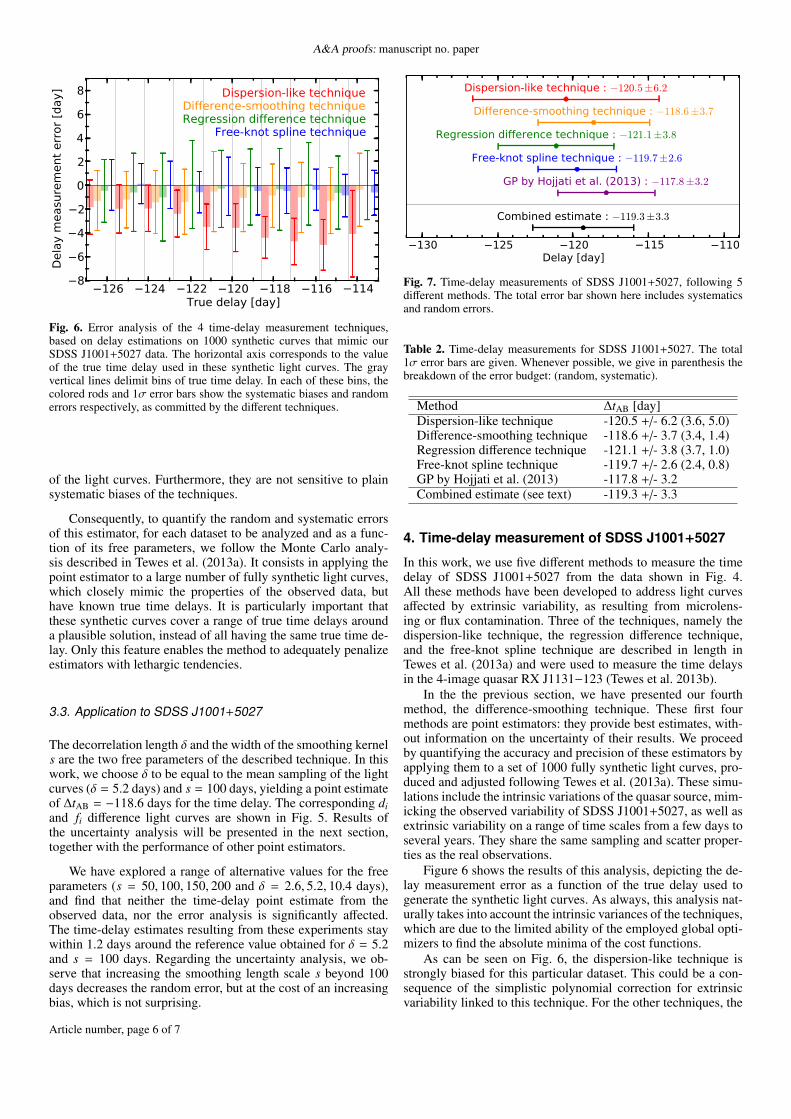
Fig. 6. Error analysis of the 4 time-delay measurement techniques,based on delay estimations on 1000 synthetic curves that mimic ourSDSS J1001+5027 data. The horizontal axis corresponds to the valueof the true time delay used in these synthetic light curves. The grayvertical lines delimit bins of true time delay. In each of these bins, thecolored rods and 1σ error bars show the systematic biases and randomerrors respectively, as committed by the different techniques.

of the light curves. Furthermore, they are not sensitive to plainsystematic biases of the techniques.

Consequently, to quantify the random and systematic errorsof this estimator, for each dataset to be analyzed and as a func-tion of its free parameters, we follow the Monte Carlo analy-sis described in Tewes et al. (2013a). It consists in applying thepoint estimator to a large number of fully synthetic light curves,which closely mimic the properties of the observed data, buthave known true time delays. It is particularly important thatthese synthetic curves cover a range of true time delays arounda plausible solution, instead of all having the same true time de-lay. Only this feature enables the method to adequately penalizeestimators with lethargic tendencies.

3.3. Application to SDSS J1001+5027

The decorrelation length δ and the width of the smoothing kernels are the two free parameters of the described technique. In thiswork, we choose δ to be equal to the mean sampling of the lightcurves (δ = 5.2 days) and s = 100 days, yielding a point estimateof ∆tAB = −118.6 days for the time delay. The corresponding diand fi difference light curves are shown in Fig. 5. Results ofthe uncertainty analysis will be presented in the next section,together with the performance of other point estimators.

We have explored a range of alternative values for the freeparameters (s = 50, 100, 150, 200 and δ = 2.6, 5.2, 10.4 days),and find that neither the time-delay point estimate from theobserved data, nor the error analysis is significantly affected.The time-delay estimates resulting from these experiments staywithin 1.2 days around the reference value obtained for δ = 5.2and s = 100 days. Regarding the uncertainty analysis, we ob-serve that increasing the smoothing length scale s beyond 100days decreases the random error, but at the cost of an increasingbias, which is not surprising.

130 125 120 115 110Delay [day]

Dispersion-like technique : −120.5±6.2

Difference-smoothing technique : −118.6±3.7

Regression difference technique : −121.1±3.8

Free-knot spline technique : −119.7±2.6

GP by Hojjati et al. (2013) : −117.8±3.2

Combined estimate : −119.3±3.3

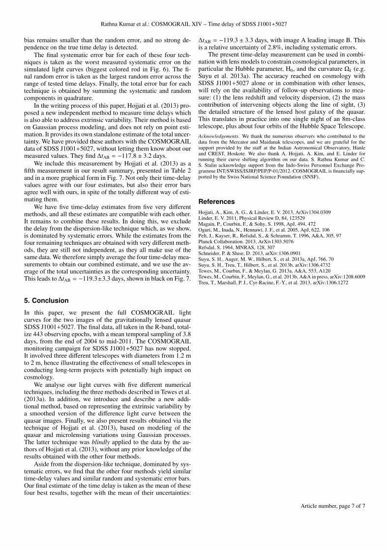
Fig. 7. Time-delay measurements of SDSS J1001+5027, following 5different methods. The total error bar shown here includes systematicsand random errors.

Table 2. Time-delay measurements for SDSS J1001+5027. The total1σ error bars are given. Whenever possible, we give in parenthesis thebreakdown of the error budget: (random, systematic).

Method ∆tAB [day]Dispersion-like technique -120.5 +/- 6.2 (3.6, 5.0)Difference-smoothing technique -118.6 +/- 3.7 (3.4, 1.4)Regression difference technique -121.1 +/- 3.8 (3.7, 1.0)Free-knot spline technique -119.7 +/- 2.6 (2.4, 0.8)GP by Hojjati et al. (2013) -117.8 +/- 3.2Combined estimate (see text) -119.3 +/- 3.3

4. Time-delay measurement of SDSS J1001+5027

In this work, we use five different methods to measure the timedelay of SDSS J1001+5027 from the data shown in Fig. 4.All these methods have been developed to address light curvesaffected by extrinsic variability, as resulting from microlens-ing or flux contamination. Three of the techniques, namely thedispersion-like technique, the regression difference technique,and the free-knot spline technique are described in length inTewes et al. (2013a) and were used to measure the time delaysin the 4-image quasar RX J1131−123 (Tewes et al. 2013b).

In the the previous section, we have presented our fourthmethod, the difference-smoothing technique. These first fourmethods are point estimators: they provide best estimates, with-out information on the uncertainty of their results. We proceedby quantifying the accuracy and precision of these estimators byapplying them to a set of 1000 fully synthetic light curves, pro-duced and adjusted following Tewes et al. (2013a). These simu-lations include the intrinsic variations of the quasar source, mim-icking the observed variability of SDSS J1001+5027, as well asextrinsic variability on a range of time scales from a few days toseveral years. They share the same sampling and scatter proper-ties as the real observations.

Figure 6 shows the results of this analysis, depicting the de-lay measurement error as a function of the true delay used togenerate the synthetic light curves. As always, this analysis nat-urally takes into account the intrinsic variances of the techniques,which are due to the limited ability of the employed global opti-mizers to find the absolute minima of the cost functions.

As can be seen on Fig. 6, the dispersion-like technique isstrongly biased for this particular dataset. This could be a con-sequence of the simplistic polynomial correction for extrinsicvariability linked to this technique. For the other techniques, the

Article number, page 6 of 7

Rathna Kumar et al.: COSMOGRAIL XIV – Time delay of SDSS J1001+5027

bias remains smaller than the random error, and no strong de-pendence on the true time delay is detected.

The final systematic error bar for each of these four tech-niques is taken as the worst measured systematic error on thesimulated light curves (biggest colored rod in Fig. 6). The fi-nal random error is taken as the largest random error across therange of tested time delays. Finally, the total error bar for eachtechnique is obtained by summing the systematic and randomcomponents in quadrature.

In the writing process of this paper, Hojjati et al. (2013) pro-posed a new independent method to measure time delays whichis also able to address extrinsic variability. Their method is basedon Gaussian process modeling, and does not rely on point esti-mation. It provides its own standalone estimate of the total uncer-tainty. We have provided these authors with the COSMOGRAILdata of SDSS J1001+5027, without letting them know about ourmeasured values. They find ∆tAB = −117.8 ± 3.2 days.

We include this measurement by Hojjati et al. (2013) as afifth measurement in our result summary, presented in Table 2and in a more graphical form in Fig. 7. Not only their time-delayvalues agree with our four estimates, but also their error barsagree well with ours, in spite of the totally different way of esti-mating them.

We have five time-delay estimates from five very differentmethods, and all these estimates are compatible with each other.It remains to combine these results. In doing this, we excludethe delay from the dispersion-like technique which, as we show,is dominated by systematic errors. While the estimates from thefour remaining techniques are obtained with very different meth-ods, they are still not independent, as they all make use of thesame data. We therefore simply average the four time-delay mea-surements to obtain our combined estimate, and we use the av-erage of the total uncertainties as the corresponding uncertainty.This leads to ∆tAB = −119.3±3.3 days, shown in black on Fig. 7.

5. Conclusion

In this paper, we present the full COSMOGRAIL lightcurves for the two images of the gravitationally lensed quasarSDSS J1001+5027. The final data, all taken in the R-band, total-ize 443 observing epochs, with a mean temporal sampling of 3.8days, from the end of 2004 to mid-2011. The COSMOGRAILmonitoring campaign for SDSS J1001+5027 has now stopped.It involved three different telescopes with diameters from 1.2 mto 2 m, hence illustrating the effectiveness of small telescopes inconducting long-term projects with potentially high impact oncosmology.

We analyse our light curves with five different numericaltechniques, including the three methods described in Tewes et al.(2013a). In addition, we introduce and describe a new addi-tional method, based on representing the extrinsic variability bya smoothed version of the difference light curve between thequasar images. Finally, we also present results obtained via thetechnique of Hojjati et al. (2013), based on modeling of thequasar and microlensing variations using Gaussian processes.The latter technique was blindly applied to the data by the au-thors of Hojjati et al. (2013), without any prior knowledge of theresults obtained with the other four methods.

Aside from the dispersion-like technique, dominated by sys-tematic errors, we find that the other four methods yield similartime-delay values and similar random and systematic error bars.Our final estimate of the time delay is taken as the mean of thesefour best results, together with the mean of their uncertainties:

∆tAB = −119.3 ± 3.3 days, with image A leading image B. Thisis a relative uncertainty of 2.8%, including systematic errors.

The present time-delay measurement can be used in combi-nation with lens models to constrain cosmological parameters, inparticular the Hubble parameter, H0, and the curvature Ωk (e.g.Suyu et al. 2013a). The accuracy reached on cosmology withSDSS J1001+5027 alone or in combination with other lenses,will rely on the availability of follow-up observations to mea-sure: (1) the lens redshift and velocity dispersion, (2) the masscontribution of intervening objects along the line of sight, (3)the detailed structure of the lensed host galaxy of the quasar.This translates in practice into one single night of an 8m-classtelescope, plus about four orbits of the Hubble Space Telescope.Acknowledgements. We thank the numerous observers who contributed to thedata from the Mercator and Maidanak telescopes, and we are grateful for thesupport provided by the staff at the Indian Astronomical Observatory, Hanleand CREST, Hoskote. We also thank A. Hojjati, A. Kim, and E. Linder forrunning their curve shifting algorithm on our data. S. Rathna Kumar and C.S. Stalin acknowledge support from the Indo-Swiss Personnel Exchange Pro-gramme INT/SWISS/ISJRP/PEP/P-01/2012. COSMOGRAIL is financially sup-ported by the Swiss National Science Foundation (SNSF).

ReferencesHojjati, A., Kim, A. G., & Linder, E. V. 2013, ArXiv1304.0309Linder, E. V. 2011, Physical Review D, 84, 123529Magain, P., Courbin, F., & Sohy, S. 1998, ApJ, 494, 472Oguri, M., Inada, N., Hennawi, J. F., et al. 2005, ApJ, 622, 106Pelt, J., Kayser, R., Refsdal, S., & Schramm, T. 1996, A&A, 305, 97Planck Collaboration. 2013, ArXiv1303.5076Refsdal, S. 1964, MNRAS, 128, 307Schneider, P. & Sluse, D. 2013, arXiv:1306.0901Suyu, S. H., Auger, M. W., Hilbert, S., et al. 2013a, ApJ, 766, 70Suyu, S. H., Treu, T., Hilbert, S., et al. 2013b, arXiv:1306.4732Tewes, M., Courbin, F., & Meylan, G. 2013a, A&A, 553, A120Tewes, M., Courbin, F., Meylan, G., et al. 2013b, A&A in press, arXiv:1208.6009Treu, T., Marshall, P. J., Cyr-Racine, F.-Y., et al. 2013, arXiv:1306.1272

Article number, page 7 of 7