xiang li, wenhao yang, shusen wang, zhihua zhang

JOURNAL OF LATEX CLASS FILES, VOL. 14, NO. 8, AUGUST 2015 1

Communication-EfficientLocal Decentralized SGD Methods

Xiang Li, Wenhao Yang, Shusen Wang, Zhihua Zhang

Abstract—Recently, the technique of local updates is a powerfultool in centralized settings to improve communication efficiencyvia periodical communication. For decentralized settings, it isstill unclear how to efficiently combine local updates and decen-tralized communication. In this work, we propose an algorithmnamed as LD-SGD, which incorporates arbitrary update schemesthat alternate between multiple Local updates and multipleDecentralized SGDs, and provide an analytical framework forLD-SGD. Under the framework, we present a sufficient conditionto guarantee the convergence. We show that LD-SGD convergesto a critical point for a wide range of update schemes when theobjective is non-convex and the training data are non-identicallyindependent distributed. Moreover, our framework brings manyinsights into the design of update schemes for decentralizedoptimization. As examples, we specify two update schemes andshow how they help improve communication efficiency. Specifi-cally, the first scheme alternates the number of local and globalupdate steps. From our analysis, the ratio of the number of localupdates to that of decentralized SGD trades off communicationand computation. The second scheme is to periodically shrinkthe length of local updates. We show that the decaying strategyhelps improve communication efficiency both theoretically andempirically.

Index Terms—Distributed Optimization, Federated Learning,Local Updates, Communication Efficiency

I. INTRODUCTION

WE study distributed optimization where the data arepartitioned among n worker nodes; the data are not

necessarily identically distributed. We seek to learn the modelparameter (aka optimization variable) x ∈ Rd by solving thefollowing distributed empirical risk minimization problem:

minx∈Rd

f(x) :=1

n

n∑k=1

fk(x), (1)

where fk(x) := Eξ∼Dk

[Fk (x; ξ)

]and Dk is the distribution

of data on the k-th node with k ∈ [n] := {1, · · · , n}. Here ξdenotes by a sample point for simplicity and can be extendedto a batch of data [1]. Such a problem is traditionally solvedunder centralized optimization paradigms such as parameterservers [2]. Federated Learning (FL), which often has a centralparameter server, enables massive edge computing devices tojointly learn a centralized model while keeping all local datalocalized [3], [4], [5], [6], [7]. As opposed to centralized

Xiang Li is with School of Mathematical Sciences, Peking University,Beijing, 100871, China. E-mail: [email protected].

Wenhao Yang is with Academy for Advanced Interdisciplinary Studies,Peking University, Beijing, 100871, China. E-mail: [email protected].

Shusen Wang is with Department of Computer Science, Stevens Institute ofTechnology, Hoboken, NJ 07030, USA. E-mail: [email protected].

Zhihua Zhang is with School of Mathematical Sciences, Peking University,Beijing, 100871, China. E-mail: [email protected].

Manuscript resubmitted March 5, 2021.

optimization, decentralized optimization lets every workernode collaborate only with their neighbors by exchanginginformation. A typical decentralized algorithm works in thisway: a node collects its neighbors’ model parameters x, takesa weighted average, and then performs a (stochastic) gradientdescent to update its local parameters [8]. Decentralized opti-mization can outperform the centralized under specific settings[8].

Decentralized optimization, as well as the centralized, suf-fers from high communication costs. The communication costis the bottleneck of distributed optimization when the numberof model parameters or the number of worker nodes are large.It is well known that deep neural networks have a large numberof parameters. For example, ResNet-50 [9] has 25 millionparameters, so sending x through a computer network canbe expensive and time-consuming. Due to modern big dataand big models, a large number of worker nodes can beinvolved in distributed optimization, which further increasesthe communication cost. The situation can be exacerbated ifworker nodes in distributed learning are remotely connected,which is the case in edge computing and other types ofdistributed learning.

In recent years, to directly save communication, manyresearchers let more local updates happen before each synchro-nization in centralized settings. A typical and famous exampleis Local SGD [4], [10], [11], [12], [13]. As its decentralizedcounterpart, Periodic Decentralized SGD (PD-SGD) alternatesbetween a fixed number of local updates and one step ofdecentralized SGD [12]. However, its update scheme is toorigid to balance the trade-off between communication andcomputation efficiently [14]. It is still unclear how to combinelocal updates and decentralized communications efficiently indecentralized settings.

To answer the question, in the paper, we propose a metaalgorithm termed as LD-SGD, which is able to incorporatearbitrary update schemes for decentralized optimization. Weprovide an analytical framework, which sheds light on the re-lationship between convergence and update schemes. We showthat LD-SGD converges with a wide choice of communicationpatterns for non-convex stochastic optimization problems andnon-identically independently distributed training data (i.e.,D1, · · · ,Dn are not the same).

We then specify two update schemes to illustrate the effec-tiveness of LD-SGD. For the first scheme, we let LD-SGDalternate (i.e., I1 steps of) multiple local updates and multiple(i.e., I2 steps of) decentralized SGDs; see the illustration inFigure 1 (b). A reasonable choice of I2 could better tradeoff the balance between communication and computation both

arX

iv:1

910.

0912

6v5

[st

at.M

L]

5 A

pr 2

021


theoretically and empirically.We observe that more local computation (i.e., large I1/I2)

often leads to higher final errors and less test accuracy. There-fore, in the second scheme, we propose and analyze a decayingstrategy that periodically halves I1. From our framework, wetheoretically verify the efficiency of the strategy. Finally, asan extension, we test LD-SGD

II. RELATED WORK

A. Decentralized stochastic gradient descent (D-SGD)

Decentralized (stochastic) algorithms were used as compro-mises when a powerful central server is not available. Theywere studied as consensus optimization in the control com-munity [15], [16], [17]. [8] justified the potential advantageof D-SGD over its centralized counterpart. D-SGD not onlyreduces the communication cost but achieves the same linearspeed-up as centralized counterparts when more nodes areavailable [8]. This promising result pushes the research ofdistributed optimization from a sheer centralized mechanismto a more decentralized pattern [18], [19], [20], [14], [21].

B. Communication efficient algorithms

The current methodology towards communication-efficiencyin distributed optimization could be roughly divided into threecategories. The most direct approach is to reduce the size ofthe messages through gradient compression or sparsification[22], [23], [24], [25], [26], [27]. An orthogonal one is to paymore local computation for less communication, e.g., one-shotaggregation [28], [29], [30], [31], [32], primal-dual algorithms[33], [34], [35] and distributed Newton methods [36], [37],[38], [39], [40]. Beyond them, a simple but powerful methodis to reduce the communication frequency by allowing morelocal updates [41], [11], [10], [42], [12], which we focus onin this paper. The last category is the push-sum methods thatis popular in control theory community [43], [44].

C. Federated optimization

The optimization problem implicit in FL is referred to asFederated Optimization (FO). One of the biggest differencethat differs FO from previous distributed optimization is thatthe training data is generated independently but according todifferent distributions. One typical optimization method forFO is is Federated Averaging (FedAvg) [45], [4], [46], whichis a centralized optimization method and is also referred toas Local SGD. In every iteration of FedAvg, a small subsetof nodes is activated, and it alternates between multiple SGDsand sends updated parameters to the central server. PD-SGD isan extension of FedAvg (or Local SGD) towards decentralizedoptimization [12], [47]. MATCHA [14] extends PD-SGD to amore federated setting by only activating a random subgraphof the network topology each round. Our work can be viewedas an attempt to generalize FedAvg to decentralized non-iidsettings.

D. Most related work

Our work is most closely related with ones in [12], [14].Specifically, [12] proposed PD-SGD that can also combinedecentralization and local updates. However, they only consid-ered the case of one step of decentralized SGD after a fixednumber of local updates. Moreover, they analyzed PD-SGDby assuming all worker nodes have access to the underlyingdistribution (hence data are identically distributed).

MATCHA [14] makes communication happen only among arandom small portion of worker nodes at each round.1 Whenno node is activated, local updates come in. Consequently,the theory of MATCHA is formulated for random connectionmatrices (i.e., W in our case) and does not straightforwardlyextend to a deterministic sequence of W. Our work mainlystudies a deterministic sequence of W but could also extendto random sequences.

III. NOTATION AND PRELIMINARIES

A. Decentralized system

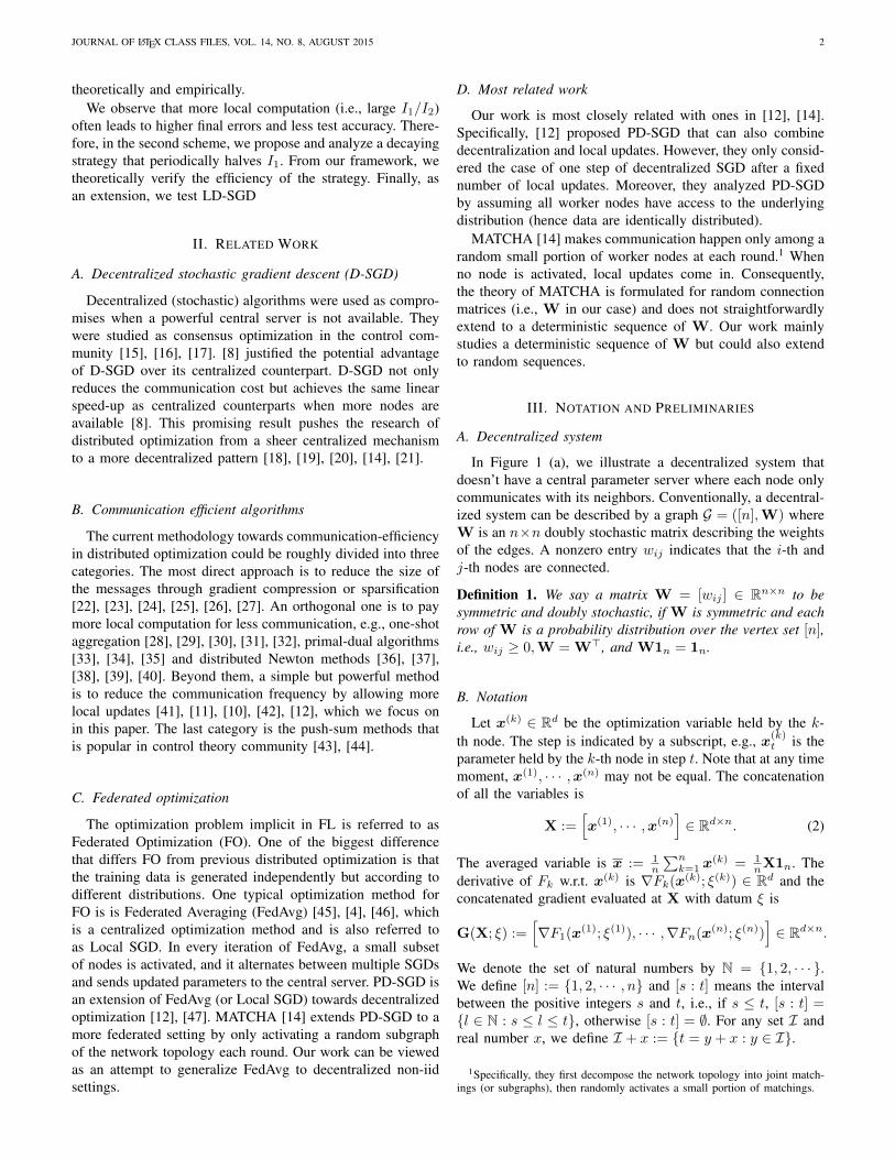
In Figure 1 (a), we illustrate a decentralized system thatdoesn’t have a central parameter server where each node onlycommunicates with its neighbors. Conventionally, a decentral-ized system can be described by a graph G = ([n],W) whereW is an n×n doubly stochastic matrix describing the weightsof the edges. A nonzero entry wij indicates that the i-th andj-th nodes are connected.

Definition 1. We say a matrix W = [wij ] ∈ Rn×n to besymmetric and doubly stochastic, if W is symmetric and eachrow of W is a probability distribution over the vertex set [n],i.e., wij ≥ 0,W = W>, and W1n = 1n.

B. Notation

Let x(k) ∈ Rd be the optimization variable held by the k-th node. The step is indicated by a subscript, e.g., x(k)

t is theparameter held by the k-th node in step t. Note that at any timemoment, x(1), · · · ,x(n) may not be equal. The concatenationof all the variables is

X :=[x(1), · · · ,x(n)

]∈ Rd×n. (2)

The averaged variable is x := 1n

∑nk=1 x

(k) = 1nX1n. The

derivative of Fk w.r.t. x(k) is ∇Fk(x(k); ξ(k)) ∈ Rd and theconcatenated gradient evaluated at X with datum ξ is

G(X; ξ) :=[∇F1(x(1); ξ(1)), · · · ,∇Fn(x(n); ξ(n))

]∈ Rd×n.

We denote the set of natural numbers by N = {1, 2, · · · }.We define [n] := {1, 2, · · · , n} and [s : t] means the intervalbetween the positive integers s and t, i.e., if s ≤ t, [s : t] ={l ∈ N : s ≤ l ≤ t}, otherwise [s : t] = ∅. For any set I andreal number x, we define I + x := {t = y + x : y ∈ I}.

1Specifically, they first decompose the network topology into joint match-ings (or subgraphs), then randomly activates a small portion of matchings.


Node 1

Node 2

Node 3

Node 5

Node 4

(a) 5 nodes in a decentralized system

Node 1

Node 2

Node 3

Node 4

Node 5

I" = 3 I% = 2

Wall clock time

(b) I1 = 3 and I2 = 2

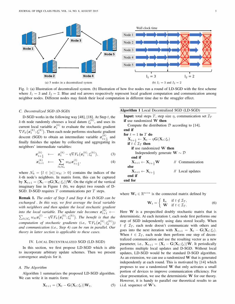
Fig. 1: (a) Illustration of decentralized system. (b) Illustration of how five nodes run a round of LD-SGD with the first schemewhere I1 = 3 and I2 = 2. Blue and red arrows respectively represent local gradient computation and communication amongneighbor nodes. Different nodes may finish their local computation in different time due to the straggler effect.

C. Decentralized SGD (D-SGD)

D-SGD works in the following way [48], [18]. At Step t, thek-th node randomly chooses a local datum ξ

(k)t , and uses its

current local variable x(k)t to evaluate the stochastic gradient

∇Fk(x

(k)t ; ξ

(k)t

). Then each node performs stochastic gradient

descent (SGD) to obtain an intermediate variable x(k)

t+ 12

andfinally finishes the update by collecting and aggregating itsneighbors’ intermediate variables:

x(k)

t+ 12

←− x(k)t − η∇Fk

(x

(k)t ; ξ

(k)t

), (3)

x(k)t+1 ←−

∑l∈Nk

wklx(l)

t+ 12

, (4)

where Nk = {l ∈ [n] |wkl > 0} contains the indices of thek-th node’s neighbors. In matrix form, this can be capturedby Xt+1 = (Xt−ηG(Xt; ξt))W. On the right of the verticalimaginary line in Figure 1 (b), we depict two rounds of D-SGD. D-SGD requires T communications per T steps.

Remak 1. The order of Step 3 and Step 4 in D-SGD can beexchanged . In this way, we first average the local variablewith neighbors and then update the local stochastic gradientinto the local variable. The update rule becomes x

(k)t+1 ←−∑

l∈Nkwklx

(l)t − η∇Fk

(x

(k)t ; ξ

(k)t

). The benefit is that the

computation of stochastic gradients (i.e., ∇Fk(x

(k)t ; ξ

(k)t

))

and communication (i.e., Step 4) can be run in parallel. Ourtheory in latter section is applicable to these cases.

IV. LOCAL DECENTRALIZED SGD (LD-SGD)

In this section, we first propose LD-SGD which is ableto incorporate arbitrary update schemes. Then we presentconvergence analysis for it.

A. The Algorithm

Algorithm 1 summarizes the proposed LD-SGD algorithm.We can write it in matrix form:

Xt+1 = (Xt −G(Xt; ξt))Wt, (5)

Algorithm 1 Local Decentralized SGD (LD-SGD)

Input: total steps T , step size η, communication set ITif use randomized W then

Compute the distribution D according to [14].end iffor t = 1 to T do

Xt+ 12← Xt − ηG(Xt; ξt)

if t ∈ IT thenif use randomized W then

Independently generate W ∼ Dend ifXt+1 ← Xt+ 1

2W // Communication

elseXt+1 ← Xt+ 1

2// Local updates

end ifend for

where Wt ∈ Rn×n is the connected matrix defined by

Wt =

{In if t /∈ IT ,W if t ∈ IT .

(6)

Here W is a prespecified doubly stochastic matrix that isdeterministic. At each iteration t, each node first performs onestep of SGD independently using data stored locally. Whent /∈ IT , each node doesn’t communicate with others andgoes into the next iteration with Xt+1 = Xt − G(Xt; ξt).When t ∈ IT , each node then perform one step of decen-tralized communication and use the resulting vector as a newparameter, i.e., Xt+1 = (Xt −G(Xt; ξt))W. It periodicallyperforms multiple local updates and D-SGD. Without localupdates, LD-SGD would be the standard D-SGD algorithm.As an extension, we can use a randomized W that is generatedindependently at each round. This is motivated by [14] whichproposes to use a randomized W that only activates a smallportion of devices to improve communication efficiency. Forclear presentation, we use the deterministic W for our theory.However, it is handy to parallel our theoretical results to ani.i.d. sequence of W’s.


Let IT index the steps where decentralized SGD is per-formed. Different choices of IT give rise to different updateschemes and then lead to different communication efficiency.For example, when we choose I0

T = {t ∈ [T ] : t mod I = 0}where I is the communication interval, LD-SGD recovers theprevious work PD-SGD [12]. Therefore, it is natural to explorehow different IT affects the convergence of LD-SGD. Ourtheory allows for arbitrary IT ⊂ [T ].

B. Convergence Analysis

1) Assumptions: In Eq. (1), we define fk(x) :=Eξ∼Dk

[Fk (x; ξ)

]as the objective function of the k-th node.

Here, x is the optimization variable and ξ is a data sample.Note that fk(x) captures the data distribution in the k-th node.We make a standard assumption: f1, · · · , fn are smooth.

Assumption 1 (Smoothness). For all k ∈ [n], fk is smoothwith modulus L, i.e.,∥∥∇fk(x)−∇fk(y)

∥∥ ≤ L∥∥x− y

∥∥, ∀ x,y ∈ Rd.

We assume bounded stochastic gradients variance, an as-sumption has been made by the prior work [8], [12], [19],[25].

Assumption 2 (Bounded variance). There exists some σ > 0such that ∀ k ∈ [n],

Eξ∼Dk

∥∥∇Fk(x; ξ)−∇fk(x)∥∥2 ≤ σ2, ∀ x ∈ Rd.

Recall from (1) that f(x) = 1n

∑nk=1 fk(x) is the global

objective function. If data distributions are not identical (Dk 6=Dl for k 6= l), then the global objective is not the same to thelocal objectives. In this case, we define κ to quantify the degreeof non-iid. If the data across nodes are iid, then κ = 0.

Assumption 3 (Degree of non-iid). There exists some κ ≥ 0such that

1

n

n∑k=1

∥∥∇fk(x)−∇f(x)∥∥2 ≤ κ2, ∀ x ∈ Rd.

Finally, we need to assume the nodes are well connected;otherwise, the update in one node cannot be propagated toanother node within a few iterations. In the worst case, if thesystem is not fully connected, the algorithm will not minimizef(x). We use ρ = |λ2| to quantify the connectivity where λ2

is the second largest absolute eigenvalue of W. A small ρindicates nice connectivity. If the connection forms a completegraph, then W = 1

n1n1>n , and thus ρ = 0.

Assumption 4 (Nice connectivity). The n × n connectivitymatrix W is symmetric doubly stochastic. Denote its eigen-values by 1 = |λ1| > |λ2| ≥ · · · ≥ |λn| ≥ 0. We assume thespectral gap 1− ρ ∈ (0, 1] where ρ = |λ2| ∈ [0, 1).

Actually, our theory can be directly extended to stochasticW, that is, at each communication round, we generate aninstance of W that conforms to a given distribution D inan independent and identical manner. For completeness, theresulting Algorithm is summarized in Algorithm ??. The onlydifference for theory is to replace ρ(W) with ρ(E

W∼DW)

and similar results follows. In experiments, we test randomW for LD-SGD following the same way as [14] did. Thisis because nodes in reality are often connected via wirelessconnections, and hence, random matrices are more realistic.

2) Main Results: Recall that xt = 1n

∑nk=1 x

(k)t is defined

as the averaged variable in the t-th iteration. Note that theobjective function f(x) is often non-convex when neuralnetworks are applied. ρs,t−1 is very important in our theorybecause it captures the characteristics of each update scheme.All the proof can be found in A.

Typically a single step of decentralized communicationpushes all local parameters to move towards their mean, butcan’t make sure they are synchronized (and identical). Thisimplies one decentralized communication happening manyiterations before will affect the current update due to suchincomplete synchronization. For example, the aggregation per-formed at iteration s will propagate the variance of stochasticgradient computed at iteration s to the current update t,incurring a multiplier to the final variance term (σ2). However,communication shrinks the effect in a exponential manner withthe exponent ρ. We capture the shrinkage effect caused bydecentralized communication starting from iteration s to t byρs,t−1.

Definition 2. For any s < t, define ρs,t−1 = ‖Φs,t−1 −1n1n1>n ‖ where Φs,t−1 =

∏t−1l=s Wl with Wl given in (6).

Actually, we have ρs,t−1 = ρ|[s:t−1]∩IT |, where [s : t − 1] ={l ∈ N : s ≤ l ≤ t− 1} and ρ is defined in Assumption 4.

Theorem 1 (LD-SGD with any IT ). Let Assumptions 1, 2, 3, 4hold and the constants L, κ, σ, and ρ be defined therein. Let∆ = f(x0)−minx f(x) be the initial error. For any fixed T ,

AT =1

T

T∑t=1

t−1∑s=1

ρ2s,t−1, BT =

1

T

T∑t=1

(t−1∑s=1

ρs,t−1

)2

,

CT = maxs∈[T−1]

T∑t=s+1

ρs,t−1

(t−1∑l=1

ρl,t−1

).

If the learning rate η is small enough such that

η < min

{1

2L,

1

4√

2L√CT

}, (7)

then

1

T

T∑t=1

E∥∥∇f(xt)

∥∥2 ≤

2∆

ηT+ηLσ2

n︸︷︷︸fully sync SGD

+ 16η2L2(ATσ

2 +BTκ2)

︸︷︷︸residual error

. (8)

The constant learning rate can be replaced by annealinglearning rate, but the convergence rate remains the same.

Corollary 1. If we choose the learning rate as η =√

nT in

Theorem 1, then when T > 4L2nmax{1, 4CT }, we have,

1

T

T∑t=1

E‖∇f(xt)‖2 ≤2∆+Lσ2

√nT

+16nL2

(ATσ

2+BTκ2)

T.

(9)


C. Sufficient condition for convergence.

If the chosen IT satisfies the sublinear condition that

AT = o(T ), BT = o(T ) and CT = o(T ), (10)

we thereby prove the convergence of LD-SGD with the updatescheme IT to a stationary point asymptotically, e.g., a localminimum or saddle point (which follows from Corollary 1).However, not every update scheme satisfies (10). For example,when IT = {T}, we have ρs,t−1 = 1 for all s < t ≤ Tand thus AT = Θ(T ), BT = Θ(T 2) and CT = Θ(T 2). ButTheorem 2 shows that as long as gap(IT ) is small enough(for example, gap(IT ) = O(T a) for some a ∈ [0, 1/2)),the sublinear condition holds. The gap indicates the largestnumber of local SGD steps before a communication roundof D-SGD is triggered. Intuitively, frequent communicationresults a small gap. So there is still a wide range of IT thatmeets the condition as long as we control the gap.

Definition 3 (Gap). For any set IT = {e1, · · · , eg} ⊂ [T ]with ei < ej for i < j, the gap of IT is defined as

gap(IT ) = maxi∈[g+1]

(ei − ei−1) (11)

where e0 = 0, eg+1 = T .

Theorem 2. Let AT , BT , CT be defined in Theorem 1. Thenfor any IT , we have

AT ≤gap(IT )

2

[1 + ρ2

1− ρ2− 1

],max{BT , CT } ≤

gap(IT )2

(1− ρ)2.

V. TWO PROPOSED UPDATE SCHEMES

Before we move to the discussion of our results, we firstspecify two classes of update schemes, both of which satisfythe sublinear condition (10). The proposed update schemesalso deepen our understandings of the main results.

A. Adding Multiple Decentralized SGDs

One centralized average can synchronize all local models,while it often needs multiple decentralized communication toachieve global consensus. Therefore, it is natural to introducemultiple decentralized SGDs (D-SGD) to I0

T . In particular, weset

I1T = {t ∈ [T ] : t mod (I1 + I2) /∈ [I1]}, (12)

where I1, I2 are parameters that respectively control the lengthof local updates and D-SGD.

Therefore, in a single round of LD-SGD, nodes performlocal updates only for a given number of “sub-rounds”, thenpreform local updates and communication for a given num-ber of other “sub-rounds”. In particular, each worker nodeperiodically alternates between two phases in a single round.In the first phase, each node locally runs I1 (I1 ≥ 0) stepsof SGD in parallel.2 In the second phase, each worker noderuns I2 (I2 ≥ 1) steps of D-SGD. As mentioned, D-SGDis a combination of (3) and (4). So communication onlyhappens in the second phase; a worker node performs I2

I1+I2T

2That is to perform (3) for I1 times.

communication per T steps. Figure 1 (b) illustrates one roundof LD-SGD with I1

T when I1 = 3 and I2 = 2. When LD-SGDis equipped with I1

T , the corresponding AT , BT , CT are O(1)w.r.t. T . The proof is provided in B.

Theorem 3 (LD-SGD with I1T ). When we set IT = I1

T forPD-SGD, under the same setting, Theorem 1 holds with

AT ≤1

2I

(1 + ρ2I2

1− ρ2I2I21 +

1 + ρ2

1− ρ2I1

)+

ρ2

1− ρ2, (13)

max {BT , CT } ≤ K2,K =I1

1− ρI2+

ρ

1− ρ. (14)

Therefore, LD-SGD converges with I1T .

The introduction of I2 extends the scope of previous frame-work: Cooperative SGD [12]. As a result, many existingalgorithms become special cases when the period lengthsI1, I2, and the connected matrix W are carefully determined.As an evident example, we recover D-SGD by setting I1 = 0and I2 > 03 and the conventional PD-SGD by setting I1 > 0and I2 = 1. Another important example is Local SGD (orFedAvg) that periodically averages local model parameters ina centralized manner [49], [10], [11], [50]. Local SGD is acase with I1 > 1, I2 = 1 and W = 1

n1n1>n . We summarizeexamples and the comparison with their convergence resultsin E.

B. Decaying the Length of Local Updates

Typically, larger local computation ratio (i.e., I1/I2) incursa higher final error, while lower local computation ratio enjoysa smaller final error but sacrifices the convergence speed. Arelated phenomena is observed by an independent work [13],which finds that a faster initial drop of global loss oftenaccompanies a higher final error.

To decay the final error, we are inspired to decay I1 everyM rounds until I1 vanishes. In this way, we use (I1, I2)for a first M rounds, then use (bI1/2c, I2) for a second Mrounds, then use (bI1/22c, I2) for a third M rounds... Werepeat this process until the J = dlog2 I1e phase where wehave bI1/2Jc = 0. To give a mathematical formulation ofsuch IT , we need an ancillary set

I(I1, I2,M) = {t ∈ [M(I1 + I2)] : t mod (I1 + I2) /∈ [I1]},

and then recursively define J0 = I(I1, I2,M) and

Jj = I(⌊

I12j

⌋, I2,M

)+ max(Jj−1), 1 ≤ j ≤ J,

where max(Jj−1) returns the maximum number collected inJj−1 and J = dlog2 I1e. Finally we set

I2T = ∪Jj=0Jj ∪ [max(JJ) : T ]. (15)

The idea is simple but the formulation is a little bit compli-cated. From the recursive definition, once t ≥ max(JJ), I1is reduced to zero and LD-SGD is reduced to D-SGD. WhenLD-SGD is equipped with I2

T , the corresponding AT , BT , CTare O(1) w.r.t. T . The proof is provided in C.

3We make a convention that [0] = ∅, so in this case I1T = [T ].


Theorem 4 (LD-SGD with I2T ). When we set IT = I2

T

for LD-SGD, under the same setting, for T ≥ max(JJ),Theorem 1 holds with

AT ≤1

T

I11−ρ2I2

ρ2(T−max(JJ )) + (1−max(JJ)

T)ρ2

1−ρ2,

BT ≤ K[

1

T

I11−ρI2

ρT−max(JJ ) + (1−max(JJ)

T)

ρ

1− ρ

],

CT ≤ K2,

where K is the same in Theorem 3. Therefore, LD-SGDconverges with I2

T .

From experiments in Section VII, the simple strategy em-pirically performs better than the PD-SGD.

VI. DISCUSSION

In this section, we will discuss some aspects of our mainresults (Theorem 1) and shed light on advantages of proposedupdate schemes.

A. Error decomposition

From Theorem 1, the upper bound (8) is decomposed intotwo parts. The first part is exactly the same as the optimizationerror bound in parallel SGD [51]. The second part is termedas residual errors as it results from performing periodic localupdates and reducing inter-node communication. In previousliterature, the application of local updates inevitably resultsthe residual error [18], [11], [12], [52], [46], [53].

To go a step further towards the residual error, take LD-SGD with I1

T for example. From Theorem 3, the residual erroroften grows with the length of local updates I = I1 + I2.When data are independently and identical distributed 4 (i.e.,κ = 0), [12] shows that the residual error of the conventionalPD-SGD grows only linearly in I . [52] achieves the similarlinear dependence on I but only requires each node drawssamples from its local partitions. When data are not identicallydistributed (i.e., κ is strictly positive), both [50] and [49] showthat the residual error of Local SGD grows quadratically in I .Theorem 3 shows that the residual error of LD-SGD with I1

T

is O(Iσ2+I2κ2), where the linear dependence comes from thestochastic gradients and the quadratic dependence results fromthe heterogeneity. The similar dependence is also establishedfor centralized momentum SGD in [53].

B. On Linear Speedup

Assume IT satisfies

AT = O(√T ) BT = O(

√T ) and CT = o(T ). (16)

Note that Condition (16) is sufficient for the sublinear condi-tion (10). From Corollary 1, the convergence of LD-SGD withIT will be dominated by the first term O( 1√

nT), when the total

step T is sufficiently large. So LD-SGD with IT can achieve alinear speedup in terms of the number of worker nodes. Both

4This is also possible if all nodes have access to the entire data, e.g.,the distributed system may shuffle data regularly so that each node actuallyoptimizes the same loss function.

of I1T and I2

T satisfy Condition (16). Taking LD-SGD withI1T for example, we have

Corollary 2. In the setting of Theorem 3, if we set η =√

nT

and choose I1, I2 to satisfy that nK2/T = 1/√nT then the

bound of 1T

∑Tt=1 E

∥∥∇f(xt)∥∥2

becomes

2∆ + Lσ2 + 4L2(σ2 + κ2)√nT

.

However, if IT fails to meet (16), the second termO(AT +BT

T · n) will dominate. As a result, more workernodes may lead to slow convergence or even divergence. Assuggested by Theorem 2, one way to make the first termdominate is to involve more communication.5

C. Communication Efficiency

LD-SGD with IT needs only |IT | communications per Ttotal steps. To increase communication efficiency, we are mo-tivated to reduce the size of IT as much as possible. However,as suggested by Theorem 2, to guarantee convergence, we arerequired to make sure IT is sufficiently large (so that gap(IT )will be small enough). The trade-off between communicationand convergence needs a careful design of update schemes.The two proposed update schemes have their own way ofbalancing the trade-off with a bounded gap(IT ).

For LD-SGD with I1T , it only needs I2

I T communicationsper T total steps where I = I1 + I2. Similar to LocalSGD which has O(T

34n

34 ) communication complexity in

centralized settings [50], LD-SGD with I1T also achieves that

level. This follows by noting from Corollary 2, to ensurenK2/T = 1/

√nT , we have I1 = (T

14n−

34 − ρ

1−ρ )(1− ρI2).Then the communication complexity of LD-SGD with I1

T is

I2

I2 + (T14n−

34 − ρ

1−ρ )(1− ρI2)T = O(T

34n

34 ),

which is an increasing function of I2 (which follows since (1−ρI2)/I2 decreases in I2 and T

14n−

34 > ρ

1−ρ for large enoughT ). Hence, large I2 increase communication cost. On the otherhand, a large I2 fastens convergence (since all bounds forAT , BT , CT in Theorem 3 are decreasing in I2). Therefore, I2helps trade-off convergence and communication (with a fixedI1). In experiments, larger I2 often results a smaller trainingloss, a higher test accuracy and a higher communication cost.The introduction of I2 allows more flexibility to balance thetrade-off between communication and convergence.

For LD-SGD with I2T , it has much faster convergence rate

since from Theorem 4, the bounds of AT and BT are muchsmaller than those of I1

T . However, it needs MI2J + (T −max(JJ)) communications per T total steps, which is morethan that of I1

T but less than that of D-SGD. Therefore, I2T

can be viewed as an intermediate state between I1T and D-

SGD. When I1 gradually vanishes, we expect that the residualerror will be reduced and better performance will follows, eventhough larger |I2

T | may increase a little bit communicationcost. From experiments in Section VII, I2

T empirically has

5By pigeonhole principle, we have gap(IT ) ≥ T|IT |+1

. In order to reducegap(IT ), one must perform more communication.


less training loss and obtains higher test accuracy than thenon-decayed LD-SGD.

D. Effect of connectivity ρ

The connectivity is measured by ρ, the second largestabsolute eigenvalue of W. The network connectivity ρ hasimpact on the convergence rate via ρs,t−1. Each update schemecorresponds to one way that ρs,t−1 depends on ρ. Generallyspeaking, well-connectivity helps reduce residual errors andthus speed up convergence. If the graph is nicely connected,in which case ρ is close to zero, then the update in onenode will be propagated to all the other nodes very soon, andthe convergence is thereby fast. As a result, the bounds inTheorem 2 are much smaller due to ρ ≈ 0. On the otherhand, if the network connection is very sparse (in which caseρ ≈ 1), ρ will greatly slows convergence. Take LD-SGD withI1T for example. When ρ ≈ 1, from Theorem 3, the bound

of AT ≈ 11−ρ

I2I2

and the bound of BT ≈ ( 11−ρ

II2

)2, both ofwhich can be extremely large. Therefore, it needs more stepsto converge.

VII. EXPERIMENTS

We evaluate LD-SGD with two proposed update schemes(I1T and I2

T ) on two tasks, namely (1) image classification onCIFAR-10 and CIFAR-100; and (2) Language modeling onPenn Treebank corpus (PTB) dataset. All training datasets areevenly partitioned over a network of workers. We will inves-tigate (i) the effect of different (I1, I2); (ii) the effect of dataheterogeneity; (iii) the effect of connected topology (differentρ); (iv) the effect of i.i.d. generated W. We run LD-SGD ina sufficient number of rounds that guarantees the convergenceof all algorithms. LD-SGD with (I1, I2) = (0, 1) is the PD-SGD. A detailed description of the training configurations isprovided in Appendix F.

a) Different I1/I2: We evaluate the performance of LD-SGD with various (I1, I2) on the three datasets. The firstcolumn of Figure 2 shows training loss v.s. epoch. Sincethe learning rate is delayed twice for image classificationtasks, there is two sudden jumps in losses for curves therein.Typically, the larger I1/I2, the larger final loss error. This isbecause, when I1/I2 is large, LD-SGD performs a relativelymany number of local computation, which would accumulatea large residual error according to our theory and thus makethe loss error larger than that of small I1/I2. However, whenwe study the optimization through the len of running time (thatis the sum of computation time and communication time), wewill find that local computation is useful in fastening realtimeconvergence and sometimes does help in better accuracy (seeFigure 7 in the Appendix). Indeed, larger I1/I2 completesthe training more earlier without degrading the accuracy toomuch. The main reason is that communication is more time-consuming than local computation, while both of them couldhelp convergence. Once we trade communication for morelocal computation, we could achieve both faster convergenceand good accuracy.

b) Same I1/I2: Then, we fix the ratio of I1/I2 andinvestigate the performance of different realizations of (I1, I2).We show the result of loss v.s. running time in the third columnof Figure 2. It seems that with the ratio I1/I2 fixed, the realtime convergence remains almost unchanged. In particular, allcurves of PTB results collapse to one single curve. It impliesthe ratio I1/I2 actually controls the communication efficiency.

c) The decay strategy.: We observe that larger I1/I2often incurs a large final error. It is intuitive to gradually decayI1/I2 until I1 reaches zero, in order to have a smaller error. Inexperiments, we heuristically halve I1 every M = 40 epochs,i.e., I1 = bI1/2c. The result of the decay strategy is shown inthe rightmost column of Figure 2. We can see that LD-SGDwith the decay strategy typically has smaller final training lossthat the non-decayed counterparts, though at the price of a littlebit communication efficiency. Clearly the decay strategy doeslower the final error and even improve the test accuracy.

d) Data heterogeneity: In previous experiments, we dis-tributed data evenly and randomly to ensure each node has(almost) iid data. We then distribute all samples in a non-i.i.d. manner and want to explore whether and how dataheterogeneity slows down convergence rate. It means κ inour theory could be very large. For image classification tasks,we evenly distribute different classes of images so that eachnode will only have samples from a same number of specificclasses.6 Therefore, the classes are not assigned uniformlyrandomly and the training data on each node is skewed. Sincelanguage itself has heterogeneity, for language modeling, wejust divide the whole dataset evenly into different nodes insteadof giving each node a copy of the whole dataset.

The result is shown in Figure 3. For a given choice of(I1, I2), we have the following observations. First, non-i.i.d.dataset often makes the training curves have larger fluctua-tion (see (b)). Second, LD-SGD converges slightly faster oni.i.d. data than on non-i.i.d. one in real time measurement(see (a), (b) and (e)). This can be explained by our theory.Data heterogeneity enlarge the quantity κ and slows downconvergence from the main theorems. Third, models trainedfrom i.i.d. datasets have slightly better generalization since itobtains slightly higher test accuracy (see (c) and (d)). Indeed,non-iid data makes the training task harder and sacrificesgeneralization a little bit. Finally, non-i.i.d. dataset often resultsin larger final training errors (see (a), (b) and (e)).

e) Different topology: In our theory, the topology affectsthe convergence rate through ρ. Smaller ρ will have smallerresidual errors and faster convergence rate. We test two graphsthat both have n = 16 nodes (see Figure 6 in the Appendixfor illustration); for Graph 1, ρ = 0.964 while for Graph 2,ρ = 0.693. With the results in Figure 4, we find that LD-SGDindeed converges slightly faster and has a higher test accuracyon Graph 2. However, in the task of Language modeling onPTD dataset, the convergence behaviors on the two graphshave little difference (see (e) in the Figure 4). We speculate thisis because language modeling is typically harder than imageclassification and is not sensitive to the underlying topology.

6After this procedure, if we has unassigned classes, we then distributedthese samples from those classes evenly and randomly into all nodes.


0 50 100 150 200epoch

10 1

100

loss

es(0,1)(10,1)(10,5)(10,10)(10,20)

(a) Loss v.s. epoch on CIFAR 10

0 500 1000 1500time

10 1

100

loss

es

(0,1)(10,1)(10,5)(10,10)(10,20)

(b) Test acc v.s. time on CIFAR 10

0 50 100 150time

100

loss

es

(3,1)(6,2)(9,3)(12,4)(15,5)

(c) Same I1/I2 on CIFAR 10

0 500 1000 1500time

10 1

100

loss

es

(10,1)(10,1)-decay(10,5)-decay(10,10)-decay(10,20)-decay

(d) Decay strategy on CIFAR 10

0 50 100 150 200epoch

10 2

10 1

100

loss

es

(0,1)(10,1)(10,5)(10,10)(10,20)

(e) Loss v.s. epoch on CIFAR 100

0 2000 4000 6000 8000 10000time

10 2

10 1

100lo

sses

(0,1)(10,1)(10,5)(10,10)(10,20)

(f) Test acc v.s. time on CIFAR 100

0 100 200 300 400time

10 1

100

loss

es

(3,1)(6,2)(9,3)(12,4)(15,5)

(g) Same I1/I2 on CIFAR 100

0 3000 6000 9000time

10 2

10 1

100

loss

es


(h) Decay strategy on CIFAR 100

0 10 20 30 40epoch

4 × 100

5 × 100

6 × 100

loss

es

(0,1)(10,1)(10,5)(10,10)(10,20)

(i) Loss v.s. epoch on PTD

0 5000 10000 15000 20000time

4 × 100

5 × 100

6 × 100

loss

es

(0,1)(10,1)(10,5)(10,10)(10,20)

(j) Test acc v.s. time on PTD

0 2000 4000 6000time

4 × 100

5 × 100

6 × 100

loss

es

(3,1)(6,2)(9,3)(12,4)(15,5)

(k) Same I1/I2 on PTD

0 5000 10000 15000time

4 × 100

5 × 100

6 × 100

loss

es


(l) Decay strategy on PTD

Fig. 2: Loss comparison on LD-SGD with different (I1, I2). The first two columns show the results of different I1/I2, the thirdcolumn shows those of the same I1/I2, and the final column shows those of the decay strategy. For test accuracy comparison,one can refer to Figure 7 in Appendix.

0 500 1000 1500time

10 1

100

loss

es

IID:(0,1)IID:(10,5)IID:(10,10)NIID:(0,1)NIID:(10,5)NIID:(10,10)

(a) Loss on CIFAR 10

0 2000 4000 6000 8000 10000time

10 2

10 1

100

loss

es


(b) Loss on CIFAR 100

0 500 1000 1500time

20

40

60

80

acc IID:(0,1)

IID:(10,5)IID:(10,10)NIID:(0,1)NIID:(10,5)NIID:(10,10)

(c) Test acc on CIFAR 10

0 2000 4000 6000 8000 10000time

0

20

40

60

acc IID:(0,1)

IID:(10,5)IID:(10,10)NIID:(0,1)NIID:(10,5)NIID:(10,10)

(d) Test acc on CIFAR 10

0 500 1000 1500 2000 2500time

4 × 100

5 × 100

6 × 100

7 × 100

loss

es


(e) Loss on PTD

Fig. 3: The effect of data heterogeneity. Non-iid data typically slows convergence rate, increases the final training error andsacrifices a little bit generalization.

f) Random W: In the body, we focus on the casewhere W is fixed and deterministic at each communicationround. MATCHA [13] proposes to improve communicationefficiency by carefully designing a random W for D-SGD.In particular, MATCHA decomposes the base communicationgraph into total several disjoint matchings and activate asmall portion of the matchings at each communication round.Mathematically speaking, MATCHA is identical to LD-SGDby letting (I1, I2) = (0, 1) and randomizing W. It is natural toapply such randomized W to LD-SGD as a further extension.In this case, W is independently generated and conforms tothe distribution D given in [13].

We then test the performance of LD-SGD with the i.i.d.generated sequence of W’s. The randomized W constructedin [13] will only activate a small portion of devices, therefore,

the straggler effect, which means some quick devices haveto wait for slower devices to response, can be alleviated. Sointuitively the communication time will be reduced.

We show the results in Figure 5. Recall that MATCHA isactually identical to LD-SGD with (I1, I2) = (0, 1) and Wrandomized. From the first row of Figure 5, LD-SGD andits variants have advantages on real time convergence thanMATCHA even a small portion of device participates in thetraining. The reason is similar as before: local updates is stillmuch cheaper than communication, even though the communi-cation is much more affordable than before by using a random-ized W. Trading local computation for less communicationis still a good strategy to improve communication efficiency.Besides, though MATCHA often has a lower training loss,LD-SGD and its variants can obtain comparative test accuracy


0 200 400 600 800time

10 1

100

loss

es1:(10,5)1:(10,5)-decay2:(10,5)2:(10,5)-decay

(a) Loss on CIFAR 10

0 500 1000 1500 2000time

10 1

100

loss

es

1:(10,5)1:(10,5)-decay2:(10,5)2:(10,5)-decay

(b) Loss on CIFAR 100

0 200 400 600 800time

20

40

60

80

acc

1:(10,5)1:(10,5)-decay2:(10,5)2:(10,5)-decay

(c) Test acc on CIFAR 10

0 500 1000 1500 2000time

0102030405060

acc

1:(10,5)1:(10,5)-decay2:(10,5)2:(10,5)-decay


0 5000 10000 15000time

3.54.04.55.05.56.06.5

loss

es

1:(10,5)1:(10,5)-decay2:(10,5)2:(10,5)-decay

(e) Loss on PTD

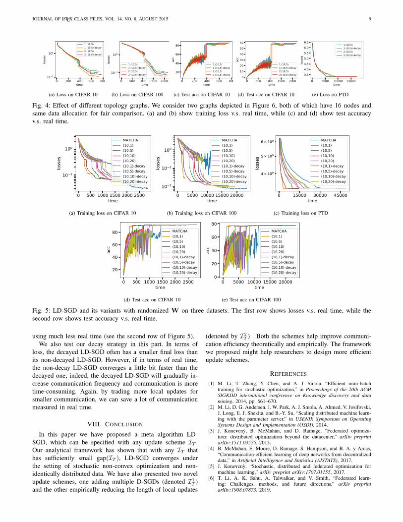
Fig. 4: Effect of different topology graphs. We consider two graphs depicted in Figure 6, both of which have 16 nodes andsame data allocation for fair comparison. (a) and (b) show training loss v.s. real time, while (c) and (d) show test accuracyv.s. real time.

0 500 1000 1500 2000 2500time

10 1

100

loss

es

MATCHA(10,1)(10,5)(10,10)(10,20)(10,1)-decay(10,5)-decay(10,10)-decay(10,20)-decay

(a) Training loss on CIFAR 10

0 5000 10000 15000 20000time

10 2

10 1

100

loss

es


(b) Training loss on CIFAR 100

0 15000 30000 45000time

4 × 100

5 × 100

6 × 100

loss

es


(c) Training loss on PTD

0 500 1000 1500 2000 2500time

20

40

60

80

acc



0 5000 10000 15000 20000time

0

20

40

60

80

acc


(e) Test acc on CIFAR 100

Fig. 5: LD-SGD and its variants with randomized W on three datasets. The first row shows losses v.s. real time, while thesecond row shows test accuracy v.s. real time.

using much less real time (see the second row of Figure 5).We also test our decay strategy in this part. In terms of

loss, the decayed LD-SGD often has a smaller final loss thanits non-decayed LD-SGD. However, if in terms of real time,the non-decay LD-SGD converges a little bit faster than thedecayed one; indeed, the decayed LD-SGD will gradually in-crease communication frequency and communication is moretime-consuming. Again, by trading more local updates forsmaller communication, we can save a lot of communicationmeasured in real time.

VIII. CONCLUSION

In this paper we have proposed a meta algorithm LD-SGD, which can be specified with any update scheme IT .Our analytical framework has shown that with any IT thathas sufficiently small gap(IT ), LD-SGD converges underthe setting of stochastic non-convex optimization and non-identically distributed data. We have also presented two novelupdate schemes, one adding multiple D-SGDs (denoted I1

T )and the other empirically reducing the length of local updates

(denoted by I2T ) . Both the schemes help improve communi-

cation efficiency theoretically and empirically. The frameworkwe proposed might help researchers to design more efficientupdate schemes.

REFERENCES

[1] M. Li, T. Zhang, Y. Chen, and A. J. Smola, “Efficient mini-batchtraining for stochastic optimization,” in Proceedings of the 20th ACMSIGKDD international conference on Knowledge discovery and datamining, 2014, pp. 661–670.

[2] M. Li, D. G. Andersen, J. W. Park, A. J. Smola, A. Ahmed, V. Josifovski,J. Long, E. J. Shekita, and B.-Y. Su, “Scaling distributed machine learn-ing with the parameter server,” in USENIX Symposium on OperatingSystems Design and Implementation (OSDI), 2014.

[3] J. Konevcny, B. McMahan, and D. Ramage, “Federated optimiza-tion: distributed optimization beyond the datacenter,” arXiv preprintarXiv:1511.03575, 2015.

[4] B. McMahan, E. Moore, D. Ramage, S. Hampson, and B. A. y Arcas,“Communication-efficient learning of deep networks from decentralizeddata,” in Artificial Intelligence and Statistics (AISTATS), 2017.

[5] J. Konevcny, “Stochastic, distributed and federated optimization formachine learning,” arXiv preprint arXiv:1707.01155, 2017.

[6] T. Li, A. K. Sahu, A. Talwalkar, and V. Smith, “Federated learn-ing: Challenges, methods, and future directions,” arXiv preprintarXiv:1908.07873, 2019.


[7] A. K. Sahu, T. Li, M. Sanjabi, M. Zaheer, A. Talwalkar, and V. Smith,“Federated optimization for heterogeneous networks,” arXiv preprintarXiv:1812.06127, 2019.

[8] X. Lian, C. Zhang, H. Zhang, C.-J. Hsieh, W. Zhang, and J. Liu, “Candecentralized algorithms outperform centralized algorithms? a case studyfor decentralized parallel stochastic gradient descent,” in Advances inNeural Information Processing Systems (NIPS), 2017.

[9] K. He, X. Zhang, S. Ren, and J. Sun, “Deep residual learning forimage recognition,” in IEEE Conference on Computer Vision and PatternRecognition (CVPR), 2016.

[10] T. Lin, S. U. Stich, and M. Jaggi, “Don’t use large mini-batches, uselocal sgd,” arXiv preprint arXiv:1808.07217, 2018.

[11] S. U. Stich, “Local SGD converges fast and communicates little,” arXivpreprint arXiv:1805.09767, 2018.

[12] J. Wang and G. Joshi, “Cooperative SGD: A unified framework for thedesign and analysis of communication-efficient SGD algorithms,” arXivpreprint arXiv:1808.07576, 2018.

[13] ——, “Adaptive communication strategies to achieve the best error-runtime trade-off in local-update sgd,” arXiv preprint arXiv:1810.08313,2018.

[14] J. Wang, A. K. Sahu, Z. Yang, G. Joshi, and S. Kar, “Matcha: Speedingup decentralized sgd via matching decomposition sampling,” arXivpreprint arXiv:1905.09435, 2019.

[15] S. S. Ram, A. Nedic, and V. V. Veeravalli, “Asynchronous gossipalgorithm for stochastic optimization: Constant stepsize analysis,” inRecent Advances in Optimization and its Applications in Engineering.Springer, 2010, pp. 51–60.

[16] K. Yuan, Q. Ling, and W. Yin, “On the convergence of decentralizedgradient descent,” SIAM Journal on Optimization, vol. 26, no. 3, pp.1835–1854, 2016.

[17] B. Sirb and X. Ye, “Consensus optimization with delayed and stochas-tic gradients on decentralized networks,” in 2016 IEEE InternationalConference on Big Data (Big Data). IEEE, 2016, pp. 76–85.

[18] G. Lan, S. Lee, and Y. Zhou, “Communication-efficient algorithms fordecentralized and stochastic optimization,” Mathematical Programming,pp. 1–48, 2017.

[19] H. Tang, X. Lian, M. Yan, C. Zhang, and J. Liu, “D2: Decentralizedtraining over decentralized data,” arXiv preprint arXiv:1803.07068,2018.

[20] A. Koloskova, S. U. Stich, and M. Jaggi, “Decentralized stochasticoptimization and gossip algorithms with compressed communication,”arXiv preprint arXiv:1902.00340, 2019.

[21] Q. Luo, J. He, Y. Zhuo, and X. Qian, “Heterogeneity-aware asyn-chronous decentralized training,” arXiv preprint arXiv:1909.08029,2019.

[22] F. Seide, H. Fu, J. Droppo, G. Li, and D. Yu, “1-bit stochastic gradientdescent and its application to data-parallel distributed training of speechDNNs,” in Fifteenth Annual Conference of the International SpeechCommunication Association, 2014.

[23] Y. Lin, S. Han, H. Mao, Y. Wang, and W. J. Dally, “Deep gradientcompression: Reducing the communication bandwidth for distributedtraining,” arXiv preprint arXiv:1712.01887, 2017.

[24] H. Zhang, J. Li, K. Kara, D. Alistarh, J. Liu, and C. Zhang, “Zipml:Training linear models with end-to-end low precision, and a little bit ofdeep learning,” in Proceedings of the 34th International Conference onMachine Learning-Volume 70. JMLR. org, 2017, pp. 4035–4043.

[25] H. Tang, S. Gan, C. Zhang, T. Zhang, and J. Liu, “Communication com-pression for decentralized training,” in Advances in Neural InformationProcessing Systems, 2018, pp. 7652–7662.

[26] H. Wang, S. Sievert, S. Liu, Z. Charles, D. Papailiopoulos, andS. Wright, “Atomo: Communication-efficient learning via atomic sparsi-fication,” in Advances in Neural Information Processing Systems, 2018,pp. 9850–9861.

[27] S. Horvath, D. Kovalev, K. Mishchenko, S. Stich, and P. Richtarik,“Stochastic distributed learning with gradient quantization and variancereduction,” arXiv preprint arXiv:1904.05115, 2019.

[28] Y. Zhang, J. C. Duchi, and M. J. Wainwright, “Communication-efficientalgorithms for statistical optimization,” Journal of Machine LearningResearch, vol. 14, pp. 3321–3363, 2013.

[29] Y. Zhang, J. Duchi, and M. Wainwright, “Divide and conquer kernelridge regression: a distributed algorithm with minimax optimal rates,”Journal of Machine Learning Research, vol. 16, pp. 3299–3340, 2015.

[30] J. D. Lee, Q. Liu, Y. Sun, and J. E. Taylor, “Communication-efficientsparse regression,” The Journal of Machine Learning Research, vol. 18,no. 1, pp. 115–144, 2017.

[31] S.-B. Lin, X. Guo, and D.-X. Zhou, “Distributed learning with regu-larized least squares,” Journal of Machine Learning Research, vol. 18,no. 1, pp. 3202–3232, 2017.

[32] S. Wang, “A sharper generalization bound for divide-and-conquer ridgeregression,” in The Thirty-Third AAAI Conference on Artificial Intelli-gence (AAAI), 2019.

[33] V. Smith, S. Forte, C. Ma, M. Takac, M. I. Jordan, and M. Jaggi,“CoCoA: A general framework for communication-efficient distributedoptimization,” arXiv preprint arXiv:1611.02189, 2016.

[34] V. Smith, C.-K. Chiang, M. Sanjabi, and A. S. Talwalkar, “Federatedmulti-task learning,” in Advances in Neural Information ProcessingSystems (NIPS), 2017.

[35] M. Hong, M. Razaviyayn, and J. Lee, “Gradient primal-dual algorithmconverges to second-order stationary solution for nonconvex distributedoptimization over networks,” in International Conference on MachineLearning (ICML), 2018.

[36] O. Shamir, N. Srebro, and T. Zhang, “Communication-efficient dis-tributed optimization using an approximate Newton-type method,” inInternational conference on machine learning (ICML), 2014.

[37] Y. Zhang and X. Lin, “DiSCO: distributed optimization for self-concordant empirical loss,” in International Conference on MachineLearning (ICML), 2015.

[38] S. J. Reddi, J. Konecny, P. Richtarik, B. Poczos, and A. Smola,“AIDE: fast and communication efficient distributed optimization,”arXiv preprint arXiv:1608.06879, 2016.

[39] Shusen Wang, Farbod Roosta Khorasani, Peng Xu, and Michael W. Ma-honey, “GIANT: Globally improved approximate newton method for dis-tributed optimization,” in Conference on Neural Information ProcessingSystems (NeurIPS), 2018.

[40] D. Mahajan, N. Agrawal, S. S. Keerthi, S. Sellamanickam, and L. Bot-tou, “An efficient distributed learning algorithm based on effective localfunctional approximations,” Journal of Machine Learning Research,vol. 19, no. 1, pp. 2942–2978, 2018.

[41] M. Zinkevich, M. Weimer, L. Li, and A. J. Smola, “Parallelized stochas-tic gradient descent,” in Advances in neural information processingsystems, 2010, pp. 2595–2603.

[42] Y. You, Z. Zhang, C.-J. Hsieh, J. Demmel, and K. Keutzer, “Imagenettraining in minutes,” in Proceedings of the 47th International Conferenceon Parallel Processing. ACM, 2018, p. 1.

[43] M. Assran, N. Loizou, N. Ballas, and M. Rabbat, “Stochastic gradientpush for distributed deep learning,” in International Conference onMachine Learning, 2019, pp. 344–353.

[44] J. Wang, V. Tantia, N. Ballas, and M. Rabbat, “Slowmo: Improvingcommunication-efficient distributed sgd with slow momentum,” arXivpreprint arXiv:1910.00643, 2019.

[45] J. Konecny, H. B. McMahan, D. Ramage, and P. Richtarik, “Federatedoptimization: distributed machine learning for on-device intelligence,”arXiv preprint arXiv:1610.02527, 2016.

[46] X. Li, K. Huang, W. Yang, S. Wang, and Z. Zhang, “On the convergenceof FedAvg on Non-IID data,” arXiv:1907.02189, 2019.

[47] F. Haddadpour and M. Mahdavi, “On the convergence of local descentmethods in federated learning,” arXiv preprint arXiv:1910.14425, 2019.

[48] P. Bianchi, G. Fort, and W. Hachem, “Performance of a distributedstochastic approximation algorithm,” IEEE Transactions on InformationTheory, vol. 59, no. 11, pp. 7405–7418, 2013.

[49] F. Zhou and G. Cong, “On the convergence properties of a k-step averag-ing stochastic gradient descent algorithm for nonconvex optimization,”arXiv preprint arXiv:1708.01012, 2017.

[50] H. Yu, S. Yang, and S. Zhu, “Parallel restarted sgd with faster con-vergence and less communication: Demystifying why model averagingworks for deep learning,” in AAAI Conference on Artificial Intelligence,2019.

[51] L. Bottou, F. E. Curtis, and J. Nocedal, “Optimization methods for large-scale machine learning,” Siam Review, vol. 60, no. 2, pp. 223–311, 2018.

[52] F. Haddadpour, M. M. Kamani, M. Mahdavi, and V. Cadambe, “Tradingredundancy for communication: Speeding up distributed SGD for non-convex optimization,” in International Conference on Machine Learning(ICML), 2019.

[53] H. Yu, R. Jin, and S. Yang, “On the linear speedup analysis ofcommunication efficient momentum SGD for distributed non-convex op-timization,” in International Conference on Machine Learning (ICML),2019.

[54] O. Press and L. Wolf, “Using the output embedding to improve languagemodels,” arXiv preprint arXiv:1608.05859, 2016.

[55] Z. Jiang, A. Balu, C. Hegde, and S. Sarkar, “Collaborative deeplearning in fixed topology networks,” in Advances in Neural InformationProcessing Systems, 2017, pp. 5904–5914.


APPENDIX APROOF OF MAIN RESULT

A. Additional notation

In the proofs we will use the following notation. LetG(X; ξ) be defined in Section III previously. Let

g(X; ξ) :=1

nG(X; ξ) 1n =

1

n

n∑k=1

Fk(x(k); ξ(k)) ∈ Rd

be the averaged gradient. Recall from (1) the definitionfk(x) := Eξ∼Dk

[Fk (x; ξ)

]. We analogously define

∇f(X) := E[G(X; ξ)

]=[∇f1(x(1)), · · · ,∇fn(x(n))

]∈ Rd×n,

∇f(X) := E[g(X; ξ)

]=

1

n∇f(X)1n =

1

n

n∑k=1

∇fk(x(k)) ∈ Rd,

∇f(x) := ∇f(x) =1

n

n∑k=1

∇fk(x) ∈ Rd.

Let Q = 1n1n1>n and xt = 1

n

∑nk=1 x

(k)t . Define the residual

error as

Vt = Eξ1

n

∥∥Xt(I−Q)∥∥2

F= Eξ

1

n

n∑k=1

∥∥x(k)t − xt

∥∥2. (17)

where the expectation is taken with respect to all randomnessof stochastic gradients or equivalently ξ = (ξ1, · · · , ξt, · · · )where ξs = (ξ

(1)s , · · · , ξ(n)

s )> ∈ Rn. Except where noted, wewill use notation E(·) in stead of Eξ(·) for simplicity. HenceVt = 1

nE∑nk=1

∥∥x(k)t − xt

∥∥2.

As mentioned in Section III, LD-SGD with arbitrary updatescheme can be equivalently written in matrix form whichwill be used repeatedly in the following convergence analysis.Specifically,

Xt+1 = (Xt −G(Xt; ξt))Wt (18)

where Xt ∈ Rd×n is the concatenation of {x(k)t }nk=1,

G(Xt; ξt) ∈ Rd×n is the concatenated gradient evaluatedat Xt with the sampled datum ξt, and Wt ∈ Rn×n is theconnected matrix defined by

Wt =

{In if t /∈ IT ;W if t ∈ IT .

(19)

B. Useful lemmas

The main idea of proof is to express Xt in terms ofgradients and then develop upper bound on residual errors.The technique to bound residual errors can be found in [13],[12], [14], [50], [53].

Lemma 1 (One step recursion). Let Assumptions 1 and 2 holdand L and σ be defined therein. Let η be the learning rate.Then the iterate obtained from the update rule (18) satisfies

E[f(xt+1)

]≤ E

[f(xt)

]− η

2(1− ηL)E

∥∥∇f(Xt)∥∥2

− η

2E∥∥∇f(xt)

∥∥2+Lσ2η2

2n+ηL2

2Vt, (20)

where the expectations are taken with respect to all random-ness in stochastic gradients.

Proof. Recall that from the update rule (18) we have

xt+1 = xt − ηg(Xt, ξt).

When Assumptions 1 and 2 hold, it follows directly fromLemma 8 in [19] that

E[f(xt+1)

]≤ E

[f(xt)

]− η

2E∥∥∇f(xt)

∥∥2

− η

2(1− ηL)E

∥∥∇f(Xt)∥∥2

+Lσ2η2

2n

+η

2E∥∥∇f(xt)−∇f(Xt)

∥∥2.

The conclusion then follows from

E‖∇f(xt)−∇f(Xt)‖2 =1

n2E∥∥∥∥ n∑k=1

[fk(xt)− fk

(x

(k)t

)] ∥∥∥∥2

(a)

≤ 1

n

n∑k=1

E∥∥∥fk(xt)− fk(x(k)

t

)∥∥∥2

(b)

≤ L2

n

n∑k=1

E∥∥x(k)

t − xt∥∥2

= L2Vt

where (a) follows from Jensen’s inequality, (b) follows fromAssumption 1, and Vt is defined in (17).

Lemma 2 (Residual error decomposition). Let X1 = x11>n ∈

Rd×n be the initialization. If we apply the update rule (18),then for any t ≥ 2,

Xt(In −Q) = −ηt−1∑s=1

G(Xs; ξs) (Φs,t−1 −Q) (21)

where Φs,t−1 is defined in (22) and Wt is given in (19).

Φs,t−1 =

{In if s ≥ t∏t−1l=s Wl if s < t.

(22)

Proof. For convenience, we denote by Gt = G(Xt; ξt) ∈Rd×n the concatenation of stochastic gradients at iteration t.According to the update rule, we have

Xt(In −Q) = (Xt−1 − ηGt−1)Wt−1(In −Q)

(a)= Xt−1(In −Q)Wt−1 − ηGt−1(Wt−1 −Q)

(b)= Xt−l(In −Q)

t−1∏s=t−l

Ws − ηt−1∑s=t−l

Gs(Φs,t−1 −Q)

(c)= X1(In −Q)Φ1,t−1 − η

t−1∑s=1

Gs (Φs,t−1 −Q)

where (a) follows from Wt−1Q = QWt−1; (b) results byiteratively expanding the expression of Xs from s = t − 1to s = t − l + 1 and plugging in the definition of Φs,t−1

in (19); (c) follows simply by setting l = t − 1. Finally, theconclusion follows from the initialization X1 = x11

>n which

implies X1(I−Q) = 0.


Lemma 3 (Gradient variance decomposition). Given anysequence of deterministic matrices {As}ts=1, then for anyt ≥ 1,

Eξ∥∥∥∥ t∑s=1

[G(Xs; ξs

)−∇f

(Xs

)]As

∥∥∥∥2

F

=

t∑s=1

Eξs∥∥∥ [G(Xs; ξs

)−∇f

(Xs

)]As

∥∥∥2

F. (23)

where the expectation Eξ(·) is taken with respect to therandomness of ξ = (ξ1, · · · , ξt, · · · ) and Eξs(·) is with respectto ξs = (ξ

(1)s , · · · , ξ(n)

s )> ∈ Rn.

Proof.

Eξ∥∥∥∥ t∑s=1

[G(Xs; ξs

)−∇f

(Xs

)]As

∥∥∥∥2

F

=

t∑s=1

Eξs∥∥∥ [G(Xs; ξs

)−∇f

(Xs

)]As

∥∥∥2

F

+ 2∑

1≤s<l≤t

Eξs,ξl[⟨ [

G(Xs; ξs

)−∇f

(Xs

)]As,

[G(Xl; ξl

)−∇f

(Xl

)]Al

⟩]where the inner product of matrix is defined by 〈A,B〉 =tr(AB>).

Since different nodes work independently without inter-ference, for s 6= l ∈ [t], ξs is independent with ξl. LetFs = σ({ξl}sl=1) be the σ-field generated by all the randomvariables until iteration s. Then for any 1 ≤ s < l ≤ t, weobtain

Eξs,ξl[⟨

(G(Xs; ξs)−∇f(Xs)) As,

(G(Xl; ξl)−∇f(Xl)) Al

⟩]= EξsEξl

[⟨(G(Xs; ξs)−∇f(Xs)) As,


⟩ ∣∣∣Fl−1

](a)= Eξs

{⟨(G(Xs; ξs)−∇f(Xs)) As,

Eξl[


∣∣Fl−1

]⟩}(b)= Eξs

[⟨G(Xs; ξs)−∇f(Xs), 0

⟩]= 0

where (a) follows from the tower rule by noting that Xs andξs are both Fl−1-measurable and (b) uses the fact that ξlis independent with Fs(s < l) and G(Xl; ξl) is a unbiasedestimator of ∇f(Xl).

Lemma 4 (Bound on second moments of gradients). For anyn points: {x(k)

t }nk=1, define Xt =[x

(1)t , · · · ,x(n)

t

]as their

concatenation, then under Assumption 1 and 3,1

nE∥∥∇f(Xt)

∥∥2

F≤ 8L2Vt + 4κ2 + 4E

∥∥∇f(Xt)∥∥2. (24)

Proof. By splitting ∇f(Xt) into four terms, we obtain

E‖∇f(Xt)‖2F=E‖∇f(Xt)−∇f(xt1

>n ) +∇f(xt1

>n )−∇f(xt)1

>n

+∇f(xt)1>n −∇f(Xt)1

>n +∇f(Xt)1

>n ‖2F

(a)

≤4E‖∇f(Xt)−∇f(xt1>n )‖2F

+ 4E‖∇f(xt1>n )−∇f(xt)1

>n ‖2F

+ 4E‖∇f(xt)1>n −∇f(Xt)1

>n ‖2F + 4E‖∇f(Xt)1

>n ‖2F

(b)=4L2nVt + 4E‖∇f(xt1

>n )−∇f(xt)1

>n ‖2F

+ 4L2nVt + 4nE‖∇f(Xt)‖2(c)=8L2nVt + 4nκ2 + 4n‖∇f(Xt)‖2

where (a) follows from the basic inequality ‖∑ni=1 Ai‖2F ≤

n∑ni=1 ‖Ai‖2F ; (b) follows from the smoothness of {fk}nk=1

and f = 1n

∑nk=1 fk (Assumption 1) and the definition of Vt

in (17); (c) follows from Assumption 3 as a result of the fact‖∇f(xt1

>n )−∇f(xt)1

>n ‖2F =

∑nk=1 ‖∇fk(xt)−∇f(xt)‖2.

Lemma 5 (Bound on residual errors). Let ρs,t−1 = ‖Φs,t−1−Q‖ where Φs,t−1 is defined in (22). Then the residual errorcan be upper bounded, i.e.,

Vt ≤ 2η2Ut

where

Ut = σ2t−1∑s=1

ρ2s,t−1 +

(t−1∑s=1

ρs,t−1

)(t−1∑s=1

ρs,t−1Ls

). (25)

andLs = 8L2Vs + 4κ2 + 4E‖∇f(Xs)‖2.

Proof. Again we denote by Gt = G(Xt; ξt) for simplicity.From Lemma 2, we can obtain a closed form of Vt. Then itfollows that

nVt

= E‖Xt(I−Q)‖2F = η2E∥∥∥∥ t−1∑s=1

Gs(Φs,t−1 −Q)

∥∥∥∥2

F

= η2E∥∥∥∥ t−1∑s=1

(Gs − EGs)(Φs,t−1 −Q) +

t−1∑s=1

EGs(Φs,t−1 −Q)

∥∥∥∥2

F

(a)

≤ 2η2E∥∥∥∥ t−1∑s=1

(Gs −∇f(Xs))(Φs,t−1 −Q)

∥∥∥∥2

F

+ 2η2E∥∥∥∥ t−1∑s=1

∇f(Xs)(Φs,t−1 −Q)

∥∥∥∥2

F

(b)= 2η2E

t−1∑s=1

‖(Gs −∇f(Xs))(Φs,t−1 −Q)‖2F

+ 2η2E∥∥∥∥ t−1∑s=1

∇f(Xs)(Φs,t−1 −Q)

∥∥∥∥2

F

(c)

≤ 2η2Et−1∑s=1

‖(Gs −∇f(Xs))(Φs,t−1 −Q)‖2F

+ 2η2E

(t−1∑s=1

‖∇f(Xs)(Φs,t−1 −Q)‖F

)2


(d)

≤ 2η2Et−1∑s=1

‖Gs −∇f(Xs)‖2F ‖Φs,t−1 −Q‖2

+ 2η2E

(t−1∑s=1

‖∇f(Xs)‖F ‖(Φs,t−1 −Q)‖

)2

(e)= 2η2

t−1∑s=1

ρ2s,t−1E‖Gs −∇f(Xs)‖2F

+ 2η2E

(t−1∑s=1

ρs,t−1‖∇f(Xs)‖F

)2

(f)

≤ 2η2t−1∑s=1

ρ2s,t−1E‖Gs −∇f(Xs)‖2F

+ 2η2

(t−1∑s=1

ρs,t−1

)(t−1∑s=1

ρs,t−1E‖∇f(Xs)‖2F

)(g)

≤ 2η2t−1∑s=1

ρ2s,t−1nσ

2 + 2η2

(t−1∑s=1

ρs,t−1

)(t−1∑s=1

ρs,t−1 · nLs

)

= 2nη2

[σ2

t−1∑s=1

ρ2s,t−1 +

(t−1∑s=1

ρs,t−1

)(t−1∑s=1

ρs,t−1Ls

)]= 2nη2Ut

where (a) follows from the basic inequality ‖a + b‖2 ≤2(‖a‖2 + ‖b‖2) and EGs = ∇f(Xs); (b) followsfrom Lemma 3; (c) follows from the triangle inequality‖∑t−1s=1 As‖F ≤

∑t−1s=1 ‖As‖F ; (d) follows from the basic

inequality ‖AB‖F ≤ ‖A‖F ‖B‖ for any matrix A and B; (e)directly follows from the notation ρs,t−1 = ‖Φs,t−1 − Q‖;(f) follows from the Cauchy inequality; (g) follows fromAssumption 2 and Lemma 4.

Lemma 6 (Bound on average residual error). For any fix T ,define

AT =1

T

T∑t=1

t−1∑s=1

ρ2s,t−1, (26)

BT =1

T

T∑t=1

(t−1∑s=1

ρs,t−1

)2

, (27)

CT = maxs∈[T−1]

T∑t=s+1

ρs,t−1

(t−1∑l=1

ρl,t−1

). (28)

Assume the learning rate is so small that 16η2L2CT < 1, then

1

T

T∑t=1

Vt ≤[ATσ

2 +BTκ2 + CT

1

T

T∑t=1

E‖∇f(Xt)‖2]

· 8η2

1− 16η2L2CT

Proof. Denote by Zs = 8L2Vs + 4E‖∇f(Xs)‖2 for short.Then Ls = Zs + 4κ2. From Lemma 5, Vt ≤ 2η2Ut, then

1

T

T∑t=1

Vt ≤ 2η2 · 1

T

T∑t=1

Ut (29)

and

1

T

T∑t=1

Ut

(25)=

1

T

T∑t=1

[σ2

t−1∑s=1

ρ2s,t−1 +

(t−1∑s=1

ρs,t−1

)(t−1∑s=1

ρs,t−1Ls

)](a)= σ2 1

T

T∑t=1

t−1∑s=1

ρ2s,t−1 + 4κ2 1

T

T∑t=1

(t−1∑s=1

ρs,t−1

)2

+1

T

T∑t=1

(t−1∑l=1

ρl,t−1

)(t−1∑s=1

ρs,t−1Zs

)(b)= σ2 1

T

T∑t=1

t−1∑s=1

ρ2s,t−1 + 4κ2 1

T

T∑t=1

(t−1∑s=1

ρs,t−1

)2

+1

T

T−1∑s=1

Zs

T∑t=s+1

ρs,t−1

(t−1∑l=1

ρl,t−1

)(c)

≤ σ2AT + 4κ2BT + CT1

T

T−1∑s=1

Zs

(d)

≤ σ2AT + 4κ2BT + 8L2CT1

T

T−1∑s=1

Vs

+ 4CT1

T

T∑t=1

E‖∇f(Xt)‖2

(e)

≤ σ2AT + 4κ2BT + 16η2L2CT1

T

T∑t=1

Ut

+ 4CT1

T

T∑t=1

E‖∇f(Xt)‖2 (30)

where (a) follows from rearrangement; (b) follows from theequality that

T∑t=1

(t−1∑s=1

ρs,t−1

)(t−1∑s=1

ρs,t−1Zs

)

=

T∑t=1

(t−1∑l=1

ρl,t−1

)(T−1∑s=1

ρs,t−1Zs1{t>s}

)

=

T−1∑s=1

Zs

T∑t=s+1

ρs,t−1

(t−1∑l=1

ρl,t−1

);

(c) following from the notation (26); (d) follows from thedefinition of Zs; (e) follows from Lemma 5.

By arranging (30) and assuming the learning rate is smallenough such that 16η2L2CT < 1, then we have

1

T

T∑t=1

Ut ≤

[ATσ

2 + 4BTκ2 + 4CT

1

T

T∑t=1

E‖∇f(Xt)‖2]

· 1

1− 16η2L2CT

≤

[ATσ

2 +BTκ2 + CT

1

T

T∑t=1

E‖∇f(Xt)‖2]

· 4

1− 16η2L2CT(31)


Our conclusion then follows by combining (29) and (31).

Lemma 7 (Computation of ρs,t−1). Define ρs,t−1 = 1 forany t ≤ s and ρs,t−1 = ‖Φs,t−1 − Q‖ when s < t. Thenρs,t−1 =

∏t−1l=s ρl with ρl = ρ if l ∈ IT , else ρl = 1, where ρ

is defined in Assumption 4. As a direct consequence, ρs,t−1 =ρs,l−1ρl,t−1 for any s ≤ l ≤ t and thus ρs,t−1 = ρ|[s:t−1]∩IT |.

Proof. By definition, we have ρs,t−1 = ‖Φs,t−1 − Q‖ =‖∏t−1l=s Wl − Q‖. Since for any positive integer l, WlQ =

QWl, then Wl and Q can be simultaneously diagonalized.From this it is easy to see that ‖

∏t−1l=s Wl −Q‖ =

∏t−1l=s ρl

where ρl is the second largest absolute eigenvalue of Wl. Notethat Wl is either W or I according to the value of l as a resultof the definition (19). Hence ρl = ρ if l ∈ IT , else = 1.

C. Proof of Theorem 1

Proof. From Lemma 1, it follows that

E[f(xt+1)

]≤ E

[f(xt)

]− η

2(1− ηL)E

∥∥∇f(Xt)∥∥2

− η

2E∥∥∇f(xt)

∥∥2+Lσ2η2

2n+ηL2

2Vt.

Note that the expectation is taken with respect to all random-ness of stochastic gradients, i.e., ξ = (ξ1, ξ2. · · · ). Arrangingthis inequality, we have

E∥∥∇f(xt)

∥∥2 ≤ 2

η

{E[f(xt)

]− E

[f(xt+1)

]}+ L2Vt

− (1− ηL)E∥∥∇f(Xt)

∥∥2+Lσ2η

n. (32)

Then it follows that

1

T

T∑t=1

E‖∇f(xt)‖2

(a)

≤ 2

ηT

{E[f(x1)

]− E

[f(xT+1)

]}+Lσ2η

n

+L2

T

T∑t=1

Vt −1− ηLT

T∑t=1

E∥∥∇f(Xt)

∥∥2

(b)

≤ 2

ηT

{E[f(x1)

]− E

[f(xT+1)

]}+Lσ2η

n

− 1− ηLT

T∑t=1

E∥∥∇f(Xt)

∥∥2+

8η2L2

1− 16η2L2CT×[

ATσ2 +BTκ

2 + CT1

T

T∑t=1

E‖∇f(Xt)‖2]

(c)

≤ 2

ηT

{E[f(x1)

]− E

[f(xT+1)

]}+Lσ2η

n+ 16η2L2ATσ

2 + 16η2L2BTκ2

− (1− ηL− 16η2L2CT )1

T

T∑t=1

E‖∇f(Xt)‖2

(d)

≤ 2

ηT

{E[f(x1)

]− E

[f(xT+1)

]}+Lσ2η

n

+ 16η2L2ATσ2 + 16η2L2BTκ

2 (33)

where (a) follows by telescoping and averaging (32); (b)follows from the upper bound of 1

T

∑Tt=1 Vt in Lemma 6;

(c) follows from the choice of the learning rate η whichsatisfies 1

1−16η2L2CT≤ 2 (since 16η2L2CT ≤ 1

2 from (7)) andrearrangement; (d) follows the requirement that the learningrate η is small enough such that ηL+ 16η2L2CT < 1 (whichis satisfied since ηL ≤ 1

2 and 16η2L2K2 ≤ 12 ).

D. Proof of Theorem 2

For any prescribed IT , denote by g = |IT | and IT ={e1, e2, · · · , eg} with e0 = 1 ≤ e1 < e2 < · · · < eg ≤T = eg+1. For short, we let si = ei − ei−1 for i ∈ [g + 1].Therefore, gap(IT ) = maxi∈[g+1] si from Definition 3 andT =

∑gl=0 sl+1.

Recall the definition in (26):

AT =1

T

T∑t=1

t−1∑s=1

ρ2s,t−1,

BT =1

T

T∑t=1

(t−1∑s=1

ρs,t−1

)2

,

CT = maxs∈[T−1]

T∑t=s+1

ρs,t−1

(t−1∑l=1

ρl,t−1

).

In this section, we will provide proof for the bound on AT , BTand CT in terms of gap(IT ) (Theorem 2).

Proof. Recall that from Definition 2 and Lemma 7, ρs,t−1 =ρ|[s:t−1]∩IT |, where [s : t − 1] = {l ∈ N : s ≤ l ≤ t − 1}and ρ is defined in Assumption 4. For simplicity, let ∆ =gap(IT ) = maxi∈[g] si.

Let’s first have a glance at∑t−1s=1 ρs,t−1. Without loss of

generality, we assume el < t ≤ el+1 for some l ∈ [g] ∪ {0}.There, we have

t−1∑s=1

ρs,t−1 = (t− el − 1) +

l∑i=1

siρl+1−i. (34)

As a direct result, for any t,∑t−1s=1 ρs,t−1 ≤ ∆ + ∆ ρ

1−ρ =∆

1−ρ . Similarly, by symmetry, we have for any s < T ,∑Tt=s+1 ρs,t−1 ≤ ∆

1−ρ . Therefore, we have

BT ≤(

∆

1− ρ

)2

CT ≤

(max

s∈[T−1]

T∑t=s+1

ρs,t−1

)maxt∈[T+1]

(t−1∑l=1

ρl,t−1

)=

(∆

1− ρ

)2

.

Finally, for AT , by using (34), we have

AT =1

T

T∑t=1

t−1∑s=1

ρs,t−1

=1

T

g∑l=0

el+1∑t=el+1

t−1∑s=1

ρs,t−1

=1

T

g∑l=0

el+1∑t=el+1

[(t− el − 1) +

l∑i=1

siρl+1−i

]


=1

T

g∑l=0

[sl+1(sl+1 − 1)

2+ sl+1

l∑i=1

siρl+1−i

]

≤ 1

T

g∑l=0

sl+1

(∆− 1

2+ ∆

l∑i=1

ρl+1−i

)

≤ ∆− 1

2+ ∆

ρ

1− ρ=

∆

2

1 + ρ

1− ρ− 1

2.

APPENDIX BPROOF OF LD-SGD WITH MULTIPLE D-SGDS

The task of analyzing convergence for different communi-cation schemes IT can be reduced to figure out how residualerrors are accumulated, i.e., to bound AT , BT and CT . In thissection, we are going to bound AT , BT and CT when theupdate scheme is I1

T . To that end, we first give a technicallemma, which facilitate the computation. Lemma 8 capturesthe accumulation rate of residual errors for I1

T .

A. One technical lemma

Lemma 8 (Manipulation on ρs,t−1). When IT = I1T , the

following properties hold for ρs,t−1:1) ρs,t−1 =

∏t−1l=s ρl with ρl = 1 if l mod I ∈ [I1], else

ρl = ρ where I = I1 + I2 and ρ is defined in Assump-tion 4. As a direct consequence, ρs,t−1 = ρs,l−1ρl,t−1

for any s ≤ l ≤ t.2) Define

αj =

(j+1)I∑t=jI+1

t−1∑s=1

ρs,t−1. (35)

Then for all j ≥ 0,

αj ≤1

2

(1 + ρI2

1− ρI2I21 +

1 + ρ

1− ρI1

)+ I

ρ

1− ρ. (36)

3) Define

βj =

(j+1)I∑t=jI+1

t−1∑s=1

ρ2s,t−1. (37)

Then for all j ≥ 0,

βj ≤1

2

(1 + ρ2I2

1− ρ2I2I21 +

1 + ρ2

1− ρ2I1

)+ I

ρ2

1− ρ2. (38)

4) For any t ≥ 1,∑t−1s=1 ρs,t−1 ≤ K where

K =I1

1− ρI2+

ρ

1− ρ. (39)

As a direct corollary, αj ≤ IK.5) Define

γj =

(j+1)I∑t=jI+1

(

t−1∑s=1

ρs,t−1)2. (40)

Then γj ≤ Kαj , where K is given in (39).6) Assume T = (R+ 1)I for some non-negative integer R.

Define

ws =

T∑t=s+1

ρs,t−1 (41)

Then for all s ∈ [T ], ws ≤ K where K is given in (39).

Proof. We prove these properties one by one:1) It is a direct corollary of Lemma 7.2) We now directly compute αj =

∑(j+1)It=jI+1

∑t−1s=1 ρs,t−1.

Without loss of generality, assume t = jI + i with j ≥0, 1 ≤ i ≤ I . (i) When 1 ≤ i ≤ I1 + 1, then

t−1∑s=1

ρs,t−1

= (i− 1) + I1

j−1∑r=0

ρI2(j−r) +

j−1∑r=0

I2∑l=1

ρI2(j−r)+1−l

= (i− 1) + I1ρI2 − ρI2(j+1)

1− ρI2+ρ− ρjI2+1

1− ρ

≤ (i− 1) + I1ρI2

1− ρI2+

ρ

1− ρ. (42)

(ii) When I1 + 1 ≤ i ≤ I , then

t−1∑s=1

ρs,t−1

= ρi−I1−1

[I1

j∑r=0

ρI2(j−r) +

j−1∑r=0

I2∑l=1

ρI2(j−r)+1−l

]

+

i−I1−1∑l=1

ρi−I1−l

= ρi−I1−1

[I1

1− ρI2(j+1)

1− ρI2+ρ− ρjI2+1

1− ρ

]+ρ− ρi−I1

1− ρ

= ρi−I1−1 · I11− ρI2(j+1)

1− ρI2+ρ− ρjI2+i−I1

1− ρ

≤ I1ρi−I1−1

1− ρI2+

ρ

1− ρ. (43)

Therefore, by combining (i) and (ii), we obtain

αj =

(j+1)I∑t=jI+1

t−1∑s=1

ρs,t−1

≤I1∑i=1

((i− 1) + I1

ρI2

1− ρI2+

ρ

1− ρ

)

+

I1+I2∑i=I1+1

(I1ρi−I1−1

1− ρI2+

ρ

1− ρ

)=

1

2

(1 + ρI2

1− ρI2I21 +

1 + ρ

1− ρI1

)+ I

ρ

1− ρ.

3) Note that βj’s share a similar structure with αj’s. Thuswe can apply a similar argument in the proof of (35) toprove (37). A quick consideration reveals that (37) canbe obtained by replacing ρ in (35) with ρ2.

4) Without loss of generality, assume t = jI+i with j ≥ 0and 1 ≤ i ≤ I . When 1 ≤ i ≤ I1 + 1, from (42),∑t−1s=1 ρs,t−1 ≤ (i − 1) + I1

ρI2

1−ρI2 + ρ1−ρ ≤

I11−ρI2 +

ρ1−ρ = K. When I1 + 1 ≤ i ≤ I1 + I2, from (43),∑t−1s=1 ρs,t−1 ≤ I1 ρ

i−I1−1

1−ρI2 + ρ1−ρ ≤

I11−ρI2 + ρ

1−ρ = K.


5) The result directly follows from this inequality(t−1∑s=1

ρs,t−1

)2

≤

(maxt≥1

t−1∑s=1

ρs,t−1

)·

(t−1∑s=1

ρs,t−1

)

≤ K

(t−1∑s=1

ρs,t−1

)where K is defined in (39).

6) Without loss of generality, assume s = jI + i with 0 ≤j ≤ R, 1 ≤ i ≤ I . (i) We first consider the case where1 ≤ i ≤ I1 + 1, then

ws ≤T+1∑t=s+1

ρs,t−1

= (I1 − i+ 1) +

(I1 +

ρ− ρI2+1

1− ρ

)R−j∑l=1

ρI2l +

I2∑l=1

ρl

≤ (I1 − i+ 1) +

(I1 +

ρ− ρI2+1

1− ρ

)ρI2

1− ρI2

+ρ− ρI2+1

1− ρ

≤ I11− ρI2

+ρ

1− ρ= K.

(ii) Then consider the case where I1 + 1 ≤ i ≤ I . IfR = j, then ws =

∑I−il=1 ρ

l ≤ ρ1−ρ ≤ K. If R ≥ j + 1,

then

ws ≤T+1∑t=s+1

ρs,t−1

= ρI−i+1

(I1 +

ρ− ρI2+1

1− ρ

)R−j−1∑l=0

ρI2l +

I−i+1∑l=1

ρl

≤ ρI−i+1

1− ρI2

(I1 +

ρ− ρI2+1

1− ρ

)+ρ− ρI−i+2

1− ρ

= I1ρI−i+1

1− ρI2+

ρ

1− ρ

≤ I11− ρI2

+ρ

1− ρ= K.

B. Proof of Theorem 3

Proof. Without loss of generality, we assume T is a multiplierof I , i.e., T = (R + 1)I for some positive integer R. Thisassumption will only simplify our proof but will not changethe conclusion.

For AT , by using (38) in Lemma 8, we have

AT =1

T

T∑t=1

t−1∑s=1

ρ2s,t−1

=1

(R+ 1)

R∑j=0

1

I

(j+1)I∑t=jI+1

ρ2s,t−1

=1

(R+ 1)

R∑j=0

1

Iβj

≤ 1

2I

(1 + ρ2I2

1− ρ2I2I21 +

1 + ρ2

1− ρ2I1

)+

ρ2

1− ρ2.

For BT , by using the result about γj in Lemma 8, we have

BT =1

T

T∑t=1

(t−1∑s=1

ρs,t−1

)2

=1

(R+ 1)

R∑j=0

1

I

(j+1)I∑t=jI+1

(t−1∑s=1

ρs,t−1

)2

=1

(R+ 1)

R∑j=0

1

Iγj

(a)

≤ K1

(R+ 1)

R∑j=0

1

Iαj

(b)

≤ K min

{K,

1

2I

(1 + ρI2

1− ρI2I21 +

1 + ρ

1− ρI1

)+

ρ

1− ρ

}where (a) follows the fact that γj ≤ Kαj and (b) follows thetwo bounds on αj provided in Lemma 8.

For CT , by using the results about ws and K in Lemma 8,we have

CT = maxs∈[T−1]

T∑t=s+1

ρs,t−1

(t−1∑l=1

ρl,t−1

)

≤ maxt∈T−1

T∑t=s+1

ρs,t−1

(maxl

t−1∑l=1

ρl,t−1

)

≤ K maxt∈T−1

T∑t=s+1

ρs,t−1 ≤ K2.

APPENDIX CPROOF OF THEOREM 4

In this section, we will give the convergence result ofTheorem 4 which states that the convergence will be fastenedif we use the decaying strategy I2

T . Again, by using theframework introduced in Appendix A, we only needs to givebounds for AT , BT and CT . To that end, we need a modifiedversion of Lemma 8 which reveals how the residual errors areaccumulated for I2

T .Recall that to define I2

T , we define an ancillary set

I(I1, I2,M) = {t ∈ [M(I1 + I2)] : t mod (I1 + I2) /∈ [I1]},

and then recursively define J0 = I(I1, I2,M) and

Jj = I(⌊

I12j

⌋, I2,M

)+ max(Jj−1), 1 ≤ j ≤ J

where max(Jj−1) returns the maximum number collected inJj−1 and J = dlog2 I1e. Finally we set

I2T = ∪Jj=0Jj ∪ [max(JJ) : T ].

In short, we first run M rounds of LD-SGD with parametersI1 and I2, then run another M rounds of LD-SGD withparameters b I12 c and I2, and keep this process going on until


we reach the J + 1 th run, where I1 shrinks to zero and weonly run D-SGD.

Lemma 9. Recall M is the decay interval, T the totalsteps and ρs,t−1 = ‖Φs,t−1 − Q‖ where Φs,t−1 is definedin (22) with Wt given in (19). Let I1, I2 be the initializedcommunication parameters. Assume T ≥ max max(JJ). Thenfor LD-SGD with the decaying strategy, we have that

1) 1T

∑Tt=1

∑t−1s=1 ρs,t−1 ≤ 1

TI1

1−ρI2 ρT+I2−max(JJ )−1 +

(1− max(JJ )T ) ρ

1−ρ ;2) 1

T

∑Tt=1

∑t−1s=1 ρ

2s,t−1 ≤ 1

TI1

1−ρ2I2 ρ2(T+I2−max(JJ )−1)+

(1− max(JJ )T ) ρ2

1−ρ2 ;3) For any t ≥ 1,

∑t−1s=1 ρs,t−1 ≤ K where K = I1

1−ρI2 +ρ

1−ρ ;4) For any T > s ≥ 1,

∑Tt=s+1 ρs,t−1 ≤ K.

Proof. We verify each inequality by directly computation:1) By exchanging the order of sum, we have2) One can complete the proof by replacing ρ with ρ2 in

the last argument.3) If t ∈ Jj , let t0 = max(Jj−1) (which is the largest

element in Jj−1), then we have

t−1∑s=1

ρs,t−1

(a)=

j−1∑l=0

∑s∈Jl

ρs,t0ρt0+1,t−1 +

t−1∑s=t0+1

ρs,t−1

= ρt0+1,t−1

j−1∑l=0

ρlI2MM−1∑s=0

ρsI2(⌊

I12l

⌋+ρ− ρI2+1

1− ρ

)

+

t−1∑s=t0+1

ρs,t−1

(b)

≤ ρt0+1,t−1

(1− ρkI2M

1− ρI2I1 +

ρ(1− ρkI2M )

1− ρ

)+

t−1∑s=t0+1

ρs,t−1

(c)

≤ I11− ρI2

+ρ

1− ρ= K

where (a) uses the fact that ρs,t−1 = ρs,t0ρt0+1,t−1;(b) follows from b I1

2l c ≤ I1; to obtain (c), one canconduct a similar discussion like what we have donein Lemma 8 by discussing whether t locates in the localupdate phase or the communication phrase. The caseis more complicated since we should also think aboutwhich round t locates. No matter which case here, (c)always holds.

4) The idea here is very similar to the that for the lateststatement. If s ≥ max(JJ), then

∑Tt=s+1 ρs,t−1 ≤∑∞

t=1 ρt = ρ

1−ρ ≤ K. Otherwise, local updates areinvolved in. Similarly, one can imitate what we havedone in Lemma 8 by discussing which round and whichphase s locates in. Actually, this bound is rather rough.

Proof of Theorem 4.. By Lemma 9, we have

AT =1

T

T∑t=1

t−1∑s=1

ρ2s,t−1

≤ 1

T

I11− ρ2I2

ρ2(T−max(JJ )) + (1− max(JJ)

T)

ρ2

1− ρ2

BT =1

T

T∑t=1

(t−1∑s=1

ρs,t−1

)2

≤

(maxt∈[T ]

t−1∑s=1

ρs,t−1

)· 1

T

T∑t=1

(t−1∑s=1

ρs,t−1

)

≤ K[

1

T

I11− ρI2

ρT−max(JJ ) + (1− max(JJ)

T)

ρ

1− ρ

]CT ≤

(maxt∈[T ]

t−1∑s=1

ρs,t−1

)·

(max

s∈[T−1]

T∑t=s+1

ρs,t−1

)≤ K2.

Then by combing Theorem 1, we finish the proof of Theo-rem 4.

APPENDIX DCONVERGENCE OF ANOTHER UPDATE RULE

A. Main result

For completeness, in this section, we study another updaterule in this section:

Xt+1 = XtWt − ηG(Xt; ξt) (44)

where Wt is given in (19). Since in this update rule, thestochastic gradient descent happens after each node commu-nicates with its neighbors, we call this type of update ascommunication-before. By contrast, what we have analyzedin the body of this paper is termed as communication-after. Alot of previous efforts study the communication-before updaterule, including [55], [8]. Fortunately, our framework is sopowerful that the convergence result for this new update rulecan be easily parallel.

Theorem 5 (LD-SGD with any IT and the update rule (44)).Let Assumption 1, 2, 3, 4 hold and the constants L, κ, σ, and ρbe defined therein. Let ∆ = f(x0)−minx f(x) be the initialerror. For any fixed T , define

AT =1

T

T∑t=1

t−1∑s=1

ρ2s+1,t−1,

BT =1

T

T∑t=1

(t−1∑s=1

ρs+1,t−1

)2

,

CT = maxs∈[T−1]

T∑t=s+1

ρs+1,t−1

(t−1∑l=1

ρl+1,t−1

).

If the learning rate η is small enough such that

η ≤ min

{1

2L,

1

4√

2L

√CT

}, (45)


then

1

T

T∑t=1

E∥∥∇f(xt)

∥∥2 ≤ 2∆

ηT+ηLσ2

n︸︷︷︸fully sync SGD

+4η2L2(ATσ2 + BTκ

2︸︷︷︸residual error

).

(46)

Remak 2. Comparing the difference of results between The-orem 1 and Theorem 5, one can find that only the value ofAT , BT and CT have been modified. In this way, one canparallel the conclusions derived for the update rule (18) tothose with the update rule (44) by simply substituting AT , BTand CT with AT , BT and CT .

Note that AT , BT and CT is always no less than AT , BTand CT . This indicators that the communication-after updaterule (18) converges faster than the communication-beforeupdate rule (44). As an example, we also given a counterpartof Theorem 3 in the latter section.

B. Useful lemmas and missing proof

Lemma 10 (Residual error decomposition). Let X1 =x11

>n ∈ Rd×n be the initialization, then for any t ≥ 2,

Xt(I−Q) = −ηt−1∑s=1

G(Xs; ξs) (Φs+1,t−1 −Q) (47)

where Φs,t−1 is already given in (22).

Proof. We still denote the gradient G(Xt; ξt) as Gt. Accord-ing to the update rule, we have

Xt(In −Q)

= (Xt−1Wt−1 − ηGt−1)(In −Q)

(a)= Xt−1(In −Q)Wt−1 − ηGt−1(In −Q)

(b)= Xt−l(In −Q)

t−1∏s=t−l

Ws − ηt−1∑s=t−l

Gs(Φs+1,t−1 −Q)

(c)= X1(In −Q)Φ1,t−1 − η

t−1∑s=1

Gs(Φs+1,t−1 −Q)

where (a) follows from Wt−1Q = QWt−1; (b) results byiteratively expanding the expression of Xs from s = t− 1 tos = t− l+ 1 and plugging in the definition of Φs,t−1 in (22);(c) follows simply by setting l = t−1. Finally, the conclusionfollows from the assumption X1(In −Q) = 0.

Lemma 11 (Bound on residual errors). Let ρs,t−1 =‖Φs,t−1 − Q‖ where Φs,t−1 is defined in (22). Then theresidual error can be upper bounded, i.e., Vt ≤ 2η2Ut where

Ut = σ2t−1∑s=1

ρ2s+1,t−1 +

(t−1∑s=1

ρs+1,t−1

)(t−1∑s=1

ρs+1,t−1Ls

).

where Ls = 8L2Vs + 4κ2 + 4E‖∇f(Xs)‖2.

Proof. The proof can be simply parallel by replacing ρs,t−1

with ρs+1,t−1 in Lemma 5.

The next thing is to bound the average residual error, i.e.,1T

∑Tt=1 Vt.

Lemma 12 (Bound on average residual error). For any fixedT , define

AT =1

T

T∑t=1

t−1∑s=1

ρ2s+1,t−1, (48)

BT =1

T

T∑t=1

(t−1∑s=1

ρs+1,t−1

)2

, (49)

CT = maxs∈[T−1]

T∑t=s+1

ρs+1,t−1

(t−1∑l=1

ρl+1,t−1

). (50)

Assuming the learning rate is so small that 16η2L2CT < 1,then

1

T

T∑t=1

Vt ≤

[ATσ

2 + BTκ2 + CT

1

T

T∑t=1

E‖∇f(Xt)‖2]×

8η2

1− 16η2L2CT

Proof. One can replace Lemma 5 with Lemma 11 in the proofof Lemma 6 to achieve the conclusion.

Proof of Theorem 5. To prove Theorem 5, one can simplyreplace Lemma 6 with Lemma 12 in the proof of Ap-pendix A-C.

C. Example: Results of LD-SGD with I1T and the other update

rule

In this part, we are going to bound AT , BT and CT whenthe update scheme is I1

T . The result shown below shows thesuperiority of the original update (18).

Lemma 13 (Manipulation on ρs+1,t−1). Noting thatt−1∑s=1

ρs+1,t−1 =

t∑s=2

ρs,t−1 ≤t∑

s=1

ρs,t−1 =

t−1∑s=1

ρs,t−1 + 1,

(51)When IT = I1

T , we can immediately deduce the followingproperties from Lemma 8 for ρs+1,t−1.

1) αj =∑(j+1)IjI+1

∑t−1s=1 ρs+1,t−1 ≤

12

(1+ρI2

1−ρI2 I21 + 1+ρ

1−ρI1

)+ I 1

1−ρ .

2) βj =∑(j+1)It=jI+1

∑t−1s=1 ρ

2s+1,t−1 ≤

12

(1+ρ2I2

1−ρ2I2 I21 + 1+ρ2

1−ρ2 I1

)+ I 1

1−ρ2 .

3) Let K = I11−ρI2 + 1

1−ρ = K + 1, then∑t−1s=1 ρs+1,t−1 ≤ K and αj ≤ IK.

4) γj =∑(j+1)It=jI+1(

∑t−1s=1 ρs+1,t−1)2 ≤ Kαj .

5) If T = (R + 1)I , we have ws =∑Tt=s+1 ρs+1,t−1 =

1 +∑Tt=s+2 ρs+1,t−1 = 1 + ws+1 ≤ 1 +K = K.

Theorem 6 (LD-SGD with I1T and the update rule (44)).

When we set IT = I1T for LD-SGD with update rule (44),

under the same setting, Theorem 5 holds with

AT ≤1

2I

(1 + ρ2I2

1− ρ2I2I21 +

1 + ρ2

1− ρ2I1

)+

1

1− ρ2,


max{BT , CT

}≤ K2, K =

I11− ρI2

+1

1− ρ.

Therefore, LD-SGD converges with I1T and the update

rule (44).

APPENDIX EDISCUSSION ON OTHERS’ CONVERGENCE RESULTS

As discussed in Section V, LD-SGD with the update schemeI1T incorporates many previous algorithms by setting I1, I2 andρ correspondingly. Taking the difference between the updaterule (18) and (44) into account, we could give convergenceresults for previous algorithms via Theorem 1 or Theorem 5(see Table I). In this section, we compare the result obtainedfrom our analytical framework with their original ones.

A. Convergence for PR-SGD

PR-SGD [49], [50], [53] is the special case of LD-SGDwhen I2 = 1 and ρ = 0 (i.e., W = Q = 1

n1n1>n ). [50]derives its convergence (Theorem 7) by requiring Assump-tion 5 which is definitely stronger than our Assumption 3.Roughly speaking we always have bound κ2 ≤ 4G2 since1n

∑nk=1

∥∥∇fk(x) − ∇f(x)∥∥2 ≤ 2

n

∑nk=1 ‖∇fk(x)‖2 +

2‖∇f(x)‖2 ≤ 4G2. Then our bound matches theirs up toconstant factors. Another interesting thing is in this case ourbound only depends on I1 = I − 1 while [50]’s relies on I .Though they are the same asymptotically, our refined analysisshows that the step of model averaging doesn’t account forthe accumulation of residual errors.

Assumption 5. (Bounded second moments) There are existsome G > 0 such that for all k ∈ [n],

Eξ∼Dk‖∇Fk(x; ξ)‖2 ≤ G2.

Theorem 7 ([50]). Let Assumption 1, 2 and 5 hold and L, σ,Gdefined therein. Let {xt}Tt=1 denote by the sequence obtainedby PR-SGD and ∆ = f(x0)−minx f(x) be the initial error.If 0 < η ≤ 1

L , then for all T , we have

1

T

T∑t=1

E∥∥∇f(xt)

∥∥2 ≤ 2∆

ηT+ηLσ2

n+ 4η2I2G2L2.

B. Convergence for D-SGD

D-SGD [55], [8] is the special case of LD-SGD whereI1 = 0, I2 = 1, 1 > ρ ≥ 0 and the communication-after update rule (introduced in Appendix D) is applied. Theoriginal paper [8] provides an analysis for D-SGD, whichwe simplify and translate into Theorem 8 in our notation.To guarantee convergence at a neighborhood of stationarypoints, [8] requires a smaller learning rate O( 1−ρ√

nL) than our

O( 1−ρL ). By contrast their residual error is larger than ours up

to a factor of O(n). They could achieve as similar bounds onresidual errors as ours by shrinking the learning rate, but theconvergence would be slowed down.

Theorem 8 ([8]). Let Assumption 1, 2, 3 and 4 hold andL, σ, κ defined therein. Let {xt}Tt=1 denote by the sequenceobtained by D-SGD and ∆ = f(x0)−minx f(x) be the initial

error. When the learning rate is small enough7 such that η ≤1−ρ

3√

6L1√n

, then for all T , we have

1

T

T∑t=1

E∥∥∇f(xt)

∥∥2

≤ 4∆

ηT+

2ηLσ2

n+ n

[6η2L2σ2

1− ρ2+

54η2L2κ2

(1− ρ)2

].

C. Convergence for PD-SGDThe PD-SGD is derived as a byproduct of the framework of

Cooperative SGD (C-SGD) in [12]. In that paper, [12] termsPD-SGD as Decentralized Periodic Averaging SGD (PDA-SGD). In our paper, the PD-SGD (or DPA-SGD) is the case ofLD-SGD with I1

T when I2 = 1 and 1 > ρ ≥ 0. We translatetheir original analysis into Theorem 9 for ease of comparison.

First, our residual error is exactly the same with theirsup to constant factors. Second, they didn’t consider the casewhen the data is non-identically distributed. Third, we allowmore flexible communication pattern design by introducingparameters I2.

Theorem 9 ([12]). Let Assumption 1, 2 and 4 hold andL, σ defined therein. Let {xt}Tt=1 denote by the sequenceobtained by PD-SGD and ∆ = f(x0) − minx f(x) be theinitial error. When the learning rate is small enough such thatη ≤ min{ 1

2L ,1−ρ√10LI}, then for all T , we have

1

T

T∑t=1

E∥∥∇f(xt)

∥∥2 ≤ 2∆

ηT+ηLσ2

n+η2L2σ2(

1 + ρ2

1− ρ2I−1).

APPENDIX FEXPERIMENTS DETAILS

Our experiment setting follows [14] closely and is imple-mented with PyTorch and MPI4Py. We adopt the code releasedby [32].

a) Image Classification.: CIFAR-10 and CIFAR-100consist of 60, 000 color images in 10 and 100 classes,respectively. We set the initial learning rate as 0.8 and itdecays by 10 after 100 and 150 epochs. The mini-batch sizeper worker node is 64.

b) Language Modeling.: The PTB dataset contains 923,000 training words. A two-layer LSTM with 1500 hiddennodes in each layer [54] is adopted. We set the initial learningrate as 20 and it decays by 4 when the training proceduresaturates. The mini-batch size per worker node is 10. Theembedding size is 1500. All algorithms are trained for 40epochs.

c) Machines.: The training procedure is performed ina single machine which is equipped with four GPUs (TeslaP100 PCIe 16GB). We uniformly distribute models (as wellas the associated data) into the four GPUs. Therefore, thecommunication in our paper actually means the inter-GPUcommunication. If we use a realistic wireless environment,then the communication cost will be larger than that of ourcurrent experiments. Hence, the advantage of LD-SGD in realtime will be much larger.

7In this way, their D2 ≥ 23

and D1 ≥ 14

, and this result follows fromreplacing D1, D2 with these constant lower bounds.


TABLE I: Convergence results of LD-SGD with I1T . To recover previous algorithms, I1, I2 and ρ (which is defined by

Assumption 4) are determined as following. The result is directly obtained by combining the bounds derived in Theorem 3with Theorem 1 or Theorem 5. In this table, ∆ = f(x0)−minx f(x) is the initial error, η the learning rate and I = I1 + I2.The result for D-SGD is obtained from Theorem 5 while the rest from Theorem 1.

Algorithms I1 I2 ρ σ κ Convergence Rate

SGD [51] 0 1 0 0 0 2∆ηT

+ ηLσ2

n

PR-SGD [50] ≥ 1 1 0 > 0 > 0 2∆ηT

+ ηLσ2

n+ 8η2L2σ2I1 + 16η2L2κ2I2

1

D-SGD [8] 0 1 [0, 1) > 0 > 0 2∆ηT

+ ηLσ2

n+ 16η2L2σ2

1−ρ2 + 16η2L2κ2

(1−ρ)2

PD-SGD [12] ≥ 0 1 [0, 1) > 0 0 2∆ηT

+ ηLσ2

n+ 8η2L2σ2( 1+ρ2

1−ρ2 I − 1)

0

1

23

4

5

6

7

(a) Graph 0 (ρ = 0.808)

0

1

2

3

4

5

6

7

8

9

10

11

12

13

14

15

(b) Graph 1 (ρ = 0.964)

0

1

2

3

4

5

6

7

8

9

10

11

12

13

14

15

(c) Graph 2 (ρ = 0.693)

Fig. 6: Three topologies that will be used in following experiments.

0 500 1000 1500time

20

40

60

80

acc

(0,1)(10,1)(10,5)(10,10)(10,20)

(a) different I1/I2 on CIFAR 10

0 50 100 150time

20

40

60

80

acc

(3,1)(6,2)(9,3)(12,4)(15,5)

(b) same I1/I2 on CIFAR10

0 500 1000 1500time

20

40

60

80ac

c


(c) decay strategy on CIFAR10

0 2000 4000 6000 8000 10000time

0

20

40

60

acc

(0,1)(10,1)(10,5)(10,10)(10,20)

(d) different I1/I2 on CIFAR10

0 100 200 300 400time

0

20

40

60

acc

(3,1)(6,2)(9,3)(12,4)(15,5)

(e) same I1/I2 on CIFAR100

0 3000 6000 9000time

0

20

40

60

acc


(f) decay strategy on CIFAR100

Fig. 7: Test accuracy of LD-SGD with different (I1, I2). The first column shows the results of different I1/I2, the column rowshows show those of the same I1/I2, and the rightmost column shows those of the decay strategy. The first row is the resultson CIFAR 10, while the second row in on CIFAR 100.

ACKNOWLEDGMENT

Li, Yang and Zhang have been supported by the NationalKey Research and Development Project of MOST of China(No. 2018AAA0101004), Beijing Natural Science Foundation

(Z190001) and Beijing Academy of Artificial Intelligence(BAAI).

xiang li, wenhao yang, shusen wang, zhihua zhang

Documents