Low-depth circuit ansatz for preparingcorrelated fermionic states on a quantum computer

Pierre-Luc Dallaire-Demers,1 Jonathan Romero,2 Libor Veis,3 Sukin Sim,2 and Alán Aspuru-Guzik2, 4

1Xanadu, 372 Richmond St W, Toronto, M5V 2L7, Canada2Department of Chemistry and Chemical Biology, Harvard University, Cambridge MA, 02138

3J. Heyrovský Institute of Physical Chemistry, ASCR, 18223 Prague, Czech Republic4Senior Fellow, Canadian Institute for Advanced Research, Toronto, Ontario M5G 1Z8, Canada

(Dated: January 4, 2018)

Quantum simulations are bound to be one of the main applications of near-term quantum com-puters. Quantum chemistry and condensed matter physics are expected to benefit from these tech-nological developments. Several quantum simulation methods are known to prepare a state on aquantum computer and measure the desired observables. The most resource economic procedureis the variational quantum eigensolver (VQE), which has traditionally employed unitary coupledcluster as the ansatz to approximate ground states of many-body fermionic Hamiltonians. A sig-nificant caveat of the method is that the initial state of the procedure is a single reference productstate with no entanglement extracted from a classical Hartree-Fock calculation. In this work, wepropose to improve the method by initializing the algorithm with a more general fermionic Gaus-sian state, an idea borrowed from the field of nuclear physics. We show how this Gaussian referencestate can be prepared with a linear-depth circuit of quantum matchgates. By augmenting the setof available gates with nearest-neighbor phase coupling, we generate a low-depth circuit ansatz thatcan accurately prepare the ground state of correlated fermionic systems. This extends the rangeof applicability of the VQE to systems with strong pairing correlations such as superconductors,atomic nuclei, and topological materials.

I. INTRODUCTION

The macroscopic properties of matter emerge from itsmicroscopic quantum constituents whose massive compo-nents are mostly fermions. Understanding and modelingthe behavior of a large number of interacting fermionsis a central and fundamental problem in Physics andChemistry which requires a large investment in compu-tational resources as the memory required to represent amany-body state scales exponentially with the number ofparticles. Therefore, a computer operating on quantummechanical principles have the potential to revolutionizethe simulation of quantum systems [1, 2]. Such a machinewould improve our ability to design new molecules suchas drugs and catalysts [3], build new superconducting[4–6] and topological materials and improve our under-standing of nuclear matter. Algorithm leveraging the ad-vantages of quantum computers for quantum simulationshave steadily been developed in the past two decades[4, 5, 7–20] as quantum processors are scaling in size[21–23]. Variational quantum eigensolvers (VQE) haverecently appeared as a promising class of quantum algo-rithms designed to prepare states for quantum simula-tions [17, 24, 25]. However, near-term devices will sufferfrom limited coherence as a consequence of noise and fi-nite experimental precision [26, 27]. This incentives thesearch for low-depth circuits for quantum simulations andstate preparation [28, 29].

In this paper, we present a new type of low-depth VQEansatz motivated by the Bogoliubov coupled cluster the-ory [30–32]. Our approach can be used to prepare theground state of correlated fermions with pairing interac-tions by systematically appending variational cycles com-

posed of linear-depth blocks of 2-qubit gates. In sectionII, we first review the formulation of the strong correla-tion problem for fermions in the context of second quan-tization. We then present the unitary version of Bogoli-ubov coupled cluster theory and review how the gener-alized Hartree-Fock (GHF) reference state can be com-puted as a fermionic Gaussian state. Using the theory ofmatchgates, we show how pure fermionic Gaussian statescan be exactly prepared on a quantum computer using alinear-depth circuit. Finally, we introduce the low-depthcircuit ansatz (LDCA), consisting of the previous match-gate circuit plus additional nearest-neighbor phase cou-pling. We numerically benchmark the LDCA in sectionIII for the prototypical examples of the Fermi-Hubbardmodel in condensed matter and the automerization reac-tion of cyclobutadiene in quantum chemistry, showing itspotential to describe the exact ground state of stronglycorrelated systems.

II. GENERALIZED VARIATIONAL QUANTUMEIGENSOLVER

In this section, we review and extend the theoreti-cal foundations of VQE. Specifically, in subsection IIA,we review the definition of finding the ground state offermionic Hamiltonians as found in quantum chemistry,condensed matter, and nuclear physics. In subsectionII B we introduce the Bogoliubov unitary coupled cluster(BUCC) theory as a variational ansatz to the groundstate problem. In subsection IIC we review the for-malism of the GHF theory as this is the starting pointof the BUCC optimization method as well as the new

arX

iv:1

801.

0105

3v1

[qu

ant-

ph]

3 J

an 2

018

2

method presented in the following subsection. In subsec-tion IID we show how a GHF state can be prepared ona quantum processor using matchgates and introduce aLDCA which can be used to prepare the ground state offermionic Hamiltonian with surprisingly high accuracy.Finally, in subsection II E, we outline an implementationto compute the analytical gradient of the LDCA usingquantum resources.

A. Formulation of the problem

Many systems in quantum chemistry [33], condensedmatter [34–36], and nuclear structure physics [37, 38] canbe modeled by an ensemble of interacting fermions (elec-trons, nucleons) described by a second quantized Hamil-tonian of the form

H =∑pq

(tpqa

†paq + ∆pqa

†pa†q + ∆∗pqaqap

)+∑pqrs vpqrsa

†pa†qasar

+∑pqrstu wpqrstua

†pa†qa†rauatas.

(1)

In general, the p,q,. . .,u indices run over all relevantquantum numbers (e.g. position, momentum, band num-ber, spin, angular momentum, isospin, etc) which defineM fermionic modes. The fermionic mode operators fol-low canonical anti-commutation relations

ak, a

†l

= δkl

and ak, al =a†k, a

†l

= 0. The kinetic energy terms

tpq and the interaction vpqrs are ubiquitous in most theo-ries, while pairing terms ∆pq often appear in the contextof mean-field superconductivity, and the three-body in-teraction term wpqrstu can be phenomenologically intro-duced in nuclear physics [39].

As a prerequisite to calculating various observablequantities, we are interested in finding the ground stateρ0 = |Ψ0〉 〈Ψ0| of the Hamiltonian (1) such that the en-ergy E is minimized over the set of all possible states ρin a given Hilbert space:

E0 ≡ E (ρ0)

= minρE (ρ)

= minρtr (Hρ) .

(2)

When this minimization cannot be done either ana-lytically or with numerically exact methods, we haveto resort to approximate methods such as variationalansatzes. One such ansatz, the BUCC method, is de-fined in the next subsection.

B. Bogoliubov unitary coupled cluster theory

Coupled cluster methods are used in ab initio quan-tum chemistry calculations to describe correlated many-

body states with a better accuracy than the Hartree-Fock method. Bogoliubov- and quasiparticle-based cou-pled cluster methods extends the range of applicabil-ity of those methods to systems with mean-field pairedstates [30–32]. Anticipating the implementation on quan-tum computers, we present the formalism for the uni-tary version of the Bogoliubov coupled cluster theory.We first review the Bogoliubov transformation and theparametrization of the ansatz.

The most general linear transformation acting onfermionic creation and annihilation operators that pre-serves the canonical anti-commutation relation is theBogoliubov transformation. In this transformation, thequasiparticle operators

(β†p′ ;βp′

)are related to the

single-particle operators(a†p; ap

)by a unitary matrix

β†p′ =∑p

(Upp′a

†p + Vpp′ap

)βp′ =

∑p

(U∗pp′ap + V ∗pp′a

†p

).

(3)

This transformation preserves the canonical anti-commutation relation such that

βk, β

†l

= δkl and

βk, βl =β†k, β

†l

= 0. By introducing the vec-

tor notation ~a> =(a1, . . . , aM , a

†1, . . . , a

†M

)and ~β> =(

β1, . . . , βM , β†1, . . . , β

†M

), it is easy to express (3) in ma-

trix notation as ~β = U~a where the Bogoliubov transfor-mation is unitary U−1 = U† and its matrix is definedas

U =

(U∗ V∗

V U

). (4)

The ground state of a quadratic Hamiltonian (all vpqrs =0 and wpqrstu = 0) is a product state

|Φ0〉 = C

M∏k=1

βk |vac〉 , (5)

where |vac〉 is the Fock vacuum and C is a normalizationfactor. If the ground state is not degenerate, (5) acts asa quasiparticle vacuum βj |Φ0〉 = 0.

We can define the quasiparticle cluster operator T =T1 + T2 + T3 + . . . where

T1 =∑k1k2

θk1k2β†k1β†k2

T2 =∑k1k2k3k4

θk1k2k3k4β†k1β†k2β

†k3β†k4

T3 =∑k1k2k3k4k5k6

θk1k2k3k4k5k6β†k1β†k2β

†k3β†k4β

†k5β†k6 .

(6)The θk1k2... ∈ C are variational parame-ters which are fully antisymmetric such thatθk1k2... = (−1)

ξ(P )θP (k1k2...), where ξ (P ) is the

signature of the permutation P . The BUCC ansatz isdefined as

|Ψ (Θ)〉 = ei(T (Θ)+T †(Θ)) |Φ0〉 . (7)

3

where Θ corresponds to the set of variational parametersθk1k2... and |Φ0〉 is a reference state. Since the transfor-mation is unitary |〈Ψ (Θ) |Ψ (Θ)〉| = 1, |Ψ (Θ)〉 is alwaysnormalized. The BUCC ansatz is said to be over single(BUCCS) or double excitations (BUCCSD) if the clusteroperator T is truncated at the first or second order.

To variationally optimize the BUCC ansatz, we aim tofind the angles Θ that minimize the energy

minΘ

E (Θ) = 〈Ψ (Θ)|H |Ψ (Θ)〉 (8)

subject to the constraint that the number of particles

〈N (Θ)〉 = 〈Ψ (Θ)|N |Ψ (Θ)〉

=∑Mp=1 〈Ψ (Θ)| a†pap |Ψ (Θ)〉

(9)

should be kept constant, as the quasiparticles operatorsgenerally do not preserve the total particle number. Inthe next subsection we will explicitly show how to com-pute the reference state from the generalized Hartree-Fock theory before describing the details of the imple-mentation of the quantum algorithm.

C. Generalized Hartree-Fock theory

Here we show how to obtain the Bogoliubov matrix (4)used to define the reference state (5). The method relieson the theory of fermionic Gaussian states [40, 41] forwhich we review the formalism and a method to obtainthe covariance matrix of the ground state without a self-consistent loop. Fermionic Gaussian states are a usefulstarting point for quantum simulations as they includethe family of Slater determinants from Hartree-Fock the-ory and Bardeen-Cooper-Schrieffer (BCS) states found inthe mean-field theory of superconductivity [42, 43] andcan be easily prepared on a quantum computer [44].

For M fermionic modes, it is convenient to define the2M Majorana operators

γj = γAj = a†j + aj

γj+M = γBj = −i(a†j − aj

) (10)

as the fermionic analogues of position and momentumoperators. Let’s note that we used either the extendedindex notation (from 1 to 2M) or the A,B superscriptnotation interchangeably throughout the paper to makethe equations clearer. Their commutation relation satis-fies γk, γl = 2δkl such that γ2

k = 1. It is useful to definethe vector notation ~γ> = (γ1, . . . , γM , γM+1, . . . , γ2M )and write ~γ = Ω~a where

Ω =

(1 1i1 −i1

). (11)

In this case, 1 is the M ×M identity matrix. A generalfermionic Gaussian state [40] has the form of the expo-nential of a quadratic product of fermionic operators

ρ =1

Ze−

i4~γ>G~γ , (12)

where Z is the normalization factor and G is a real andantisymmetric matrix such that G> = −G. It can befully characterized by a real and antisymmetric covari-ance matrix which is defined by

Γkl =i

2tr (ρ [γk, γl]) , (13)

where [·, ·] is the commutator. For a pure Gaussian state,Γ 2 = −1, where 1 is the 2M × 2M identity matrix. Ingeneral, the purity is given by χ = − 1

2M tr(Γ 2). In order

to extract U given a covariance matrix Γ , we make useof the complex covariance matrix representation

Γc =1

4Ω†ΓΩ∗ =

(Q RR∗ Q∗

), (14)

where Qkl = i2 〈[ak, al]〉 and Rkl = i

2

⟨[ak, a

†l

]⟩(ex-

pectation values are defined as 〈O〉 = tr (Oρ)). Fromthere, we can define the single-particle density operatorsκ ≡ −iQ and % ≡ 1

21 − iR> and recast the Gaussianstate in the form of a single-particle density matrix

M =

(% κ†

κ 1− %>)

(15)

such thatM2 =M for pure states [45]. If we define the

matrix E =

(0 00 1

), then it is possible to find the Bo-

goliubov transformation (4) with the eigenvalue equation

MU† = EU†. (16)

Next, we show how to compute the covariance matrix(13) approximating the ground state of the Hamiltonian(1).

1. Finding the ground state

These steps are a review of the method found in [41]aimed at calculating the covariance matrix approximat-ing the ground state of an interacting Hamiltonian with-out a self-consistent loop.

The Hamiltonian (1) can be rewritten with Majoranaoperators in the form

H = i∑pq Tpqγpγq

+∑pqrs Vpqrsγpγqγsγr

+i∑pqrstuWpqrstuγpγqγrγuγtγs,

(17)

4

where T> = −T and V and W are antisymmetric underthe exchange of any two adjacent indices. Expectationvalues over gaussian states can be efficiently calculatedusing Wick’s theorem which has the form

iptr(ργj1 . . . γj2p

)= Pf

(Γ |j1...j2p

), (18)

where 1 ≤ j1 < . . . < j2p ≤ 2M , Γ |j1...j2p is the corre-sponding submatrix of Γ and

Pf (Γ ) = 12MM !

∑s∈S2M

sgn (s)∏Mj=1 Γs(2j−1),s(2j)

=√

det (Γ )(19)

is the Pfaffian of a 2M × 2M matrix defined from thesymmetric group S2M where sgn (s) is the signature ofthe permutation s. Assuming that Wick’s theorem holds,we can write an effective but state dependent quadraticHamiltonian

h (Γ) = T + 6trB (V Γ) + 45trC (WΓΓ) , (20)

where trB (V Γ)ij =∑kl VijklΓlk and trC (WΓΓ)ij =∑

klmnWijklmnΓknΓml. To get the covariance matrix ofthe reference state, we use the imaginary time evolutionstarting from a pure state Γ (0)

2= −1:

Γ (τ) = O (τ) Γ (0)O (τ)>, (21)

where the orthogonal time evolution operator is given by

O (τ) = Te2∫ τ0dτ ′[h(Γ(τ ′)),Γ(τ ′)], (22)

with T being the time ordering. The steady state isreached when [h (Γ) ,Γ] = 0. This is guaranteed to lowerthe energy of an initial state and keep the purity of theinitial Γ (0) but the imaginary time evolution may getstuck in a local minimum. A second complementary ap-proach consists in minimizing the free energy of (17).The procedure simply involves fixed point iterations onthe transcendental equation

Γ = limβ→∞

tanh [2iβh (Γ)] . (23)

In our numerical experiments, we find that an imaginarytime evolution (21) followed by a fixed point evolution(23) is numerically stable and consistently reaches thedesired GHF ground state. In the following subsection,we will show how the theory of matchgates can be usedto prepare a pure Gaussian state on a quantum computeras a reference state for a variational procedure.

D. The quantum subroutine

It is expected that quantum computer will enable thesimulation of quantum systems beyond the reach of clas-sical computers. An important challenge for practical

simulations is to prepare the ground state of interest-ing Hamiltonians with high accuracy. The VQE protocol[14, 17, 24, 25, 28] suggests a general procedure to reachthis ground state. However, current implementations ofthe protocol have to trade long circuit depth for accuracyin a non-controllable manner. In this subsection, we in-troduce a composable VQE ansatz which is both accu-rate and hardware efficient with the added advantage ofbeing able to represent states with BCS-like pairing cor-relations. Our method relies on the theory of matchgatesand its relation to fermionic linear optics [44, 46–50] toboth prepare a reference Gaussian state and parametrizean ansatz with a transformation analogous to fermionicnon-linear optics. After a brief review of the theory ofmatchgates, we show how a given pure Gaussian state canbe prepared on a quantum register with a linear-depth al-gorithm. A different algorithm with the same scaling wasrecently proposed in [51]. Unlike the procedure in [51],that relies on a gate decomposition strategy, our methodhas a fixed circuit structure with variable parameters.We then proceed to introduce a low-depth circuit ansatzwith inherited properties of the BUCC ansatz and theapparent accuracy of the full configuration interactionmethod.

1. Matchgate decomposition of a Bogoliubov transformation

In the computational basis of a 2-qubit Hilbert space,matchgates [46] have the general form

G (A,B) =

p 0 0 q0 w x 00 y z 0r 0 0 s

, (24)

where A =

(p qr s

)and B =

(w xy z

)are SU (2) ma-

trices with the same determinant detA = detB. Theyform a group which is generated by the tensor productof nearest-neighbor Pauli operators

σjx ⊗ σj+1x = −iγBj γAj+1

σjx ⊗ σj+1y = −iγBj γBj+1

σjy ⊗ σj+1x = iγAj γ

Aj+1

σjy ⊗ σj+1y = iγAj γ

Bj+1

σjz ⊗ Ij+1 = −iγAj γBj

Ij ⊗ σj+1z = −iγAj+1γ

Bj+1,

(25)

which also correspond to the Jordan-Wigner transformedproduct of all products of nearest-neighbor Majoranaoperators, therefore establishing the connection withfermionic gaussian operations. The Bogoliubov transfor-mation (3) can be written as an SO (2M) transformation

5

of the Majorana operators (10) as ~γ′ = R~γ, where

R =

(Re (U + V) −Im (U−V)Im (U + V) Re (U−V)

). (26)

To implement this transformation on a quantum proces-sor, there exists a quantum circuit of nearest-neighbormatchgates UBog acting on M qubits [49] such that

UBogγjU†Bog =

2M∑k=1

Rkjγk. (27)

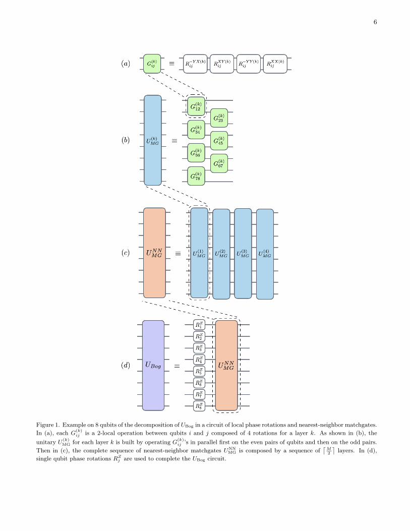
An example of such a circuit known as the fermionic fastFourier transform is described in [44]. In general, theHoffman algorithm [52] can be used to decompose UBog in2M (M − 1) SO (4) rotations between pairs of modes andM SO (2) local phases. In total, these 2M2 −M anglescorrespond to the same number of quantum gates. Usingthe fact that quantum gates can be operated in parallelin a linear chain of qubits, any transformation R can beimplemented in circuit depth 8

⌈M2

⌉+ 1, as detailed in

Figure 1.Since the Hoffman method assumes sequential opera-

tions on each pair of modes, we used an optimal controlscheme [53, 54] in SO (2M) to allow an easy parametriza-tion of gates acting in parallel. This is generally efficienton a classical computer since the matchgates only operateon a much smaller subspace of the full SU

(2M)trans-

formation allowed on M qubits. The transformation Rcan be decomposed in local and nearest-neighbor moderotations such that

R =∏dM2 ek=1

∏µ,ν

∏j∈odd r

µνj,j+1

(θµν(k)j,j+1

)×∏µ,ν

∏j∈even r

µνj,j+1

(θµν(k)j,j+1

)×∏Mj=1 r

ABjj

(θABjj

),

(28)

where µ, ν ∈ A,B and j ∈ 1, . . . ,M. The moderotations are parametrized by the 2M2−M angles θµν(k)

ij

rµνij = e2θµνij hµνij (29)

with SO (2M) Hamiltonians

hµνij = δiµ,jν − δjν,iµ. (30)

The optimal control method maximizes the fidelity func-tion

Φ =1

2MtrR>targetR (Θ)

(31)

using the gradient

∂rµνij

∂θαβkl= 2hµνij r

µνij δαµδβνδkiδlj . (32)

As shown in Figure 1 on a 8-qubit example, this decom-position explicitly translates into a quantum circuit ofsingle qubit phase-rotations

RZj = eiθABii σiz (33)

and nearest-neighbor matchgates

G(k)ij = R

XX(k)ij R

−Y Y (k)ij R

XY (k)ij R

−Y X(k)ij , (34)

where each rotation corresponds to

R−Y X(k)ij = e−iθ

AA(k)ij σiy⊗σ

jx

RXY (k)ij = eiθ

BB(k)ij σix⊗σ

jy

R−Y Y (k)ij = e−iθ

AB(k)ij σiy⊗σ

jy

RXX(k)ij = eiθ

BA(k)ij σix⊗σ

jx .

(35)

Each parallel cycle interleaves gates between even andodd nearest neighbors

U(k)MG =

∏i∈odd

G(k)i,i+1

∏i∈even

G(k)i,i+1 (36)

and there are⌈M2

⌉cycles in total:

UNNMG =

dM2 e∏k=1

U(k)MG. (37)

Finally, the unitary Bogoliubov transformation can becomposed as

UBog = UNNMG

M∏i=1

RZi (38)

and is also a gaussian operation of the form UBog =

ei∑pq τpqγpγq , where τ> = −τ . In the case where the

reference state is a Slater determinant, only number-conserving matchgates are required to prepare the stateand the depth of the circuit would scale as 4

⌈M2

⌉+ 1

(since all θAA(k)ij and θBB(k)

ij are set to zero). It should benoticed that a unitary coupled cluster ansatz truncatedat first order ei(T1(Θ)+T †1 (Θ)) is also a gaussian transfor-mation and can be implemented in the same way as UBog

with no trotterization. In what follows, we introduce aVQE scheme that builds on this observation by introduc-ing non-matchgate variational terms into a gate sequencesimilar to the UBog decomposition.

6

Figure 1. Example on 8 qubits of the decomposition of UBog in a circuit of local phase rotations and nearest-neighbor matchgates.In (a), each G

(k)ij is a 2-local operation between qubits i and j composed of 4 rotations for a layer k. As shown in (b), the

unitary U(k)MG for each layer k is built by operating G

(k)ij ’s in parallel first on the even pairs of qubits and then on the odd pairs.

Then in (c), the complete sequence of nearest-neighbor matchgates UNNMG is composed by a sequence of

⌈M2

⌉layers. In (d),

single qubit phase rotations RZj are used to complete the UBog circuit.

7

2. A low-depth circuit ansatz

The Bogoliubov transformation (38) acts as a changeof basis of the fermionic modes. Therefore, one cansimply follow the VQE protocol [14] to implement theBUCC ansatz (7) and measure the expectation values⟨H⟩

=⟨UBogHU

†Bog

⟩and

⟨N⟩

=⟨UBogNU

†Bog

⟩in the

modified basis to prepare an approximate ground stateof (1). This has the advantage of extending the range ofHamiltonians that can be processed to those with non-number conserving terms (like pairing fields) when com-pared to the traditional unitary coupled cluster ansatz.However, the change of basis may significantly increasethe number of terms that have to be measured. In orderto reduce the number of measurements in the VQE pro-tocol, one can start in the product state (5) and carryout the variational unitary (7) in the quasiparticle basis,followed by an inverse Bogoliubov transformation usingmatchgates and measurement of the expectation valuesof the Hamiltonian (1) and the number operator N in theoriginal fermionic orbital basis. In the quasiparticle basis,we can map the Bogoliubov operators to qubit operatorswith the Jordan-Wigner transformation [7, 55, 56] sincethey follow the canonical anti-commutation relation

β†p = (−1)p−1

(⊗p−1j=1 σz

)⊗ σ+

βp = (−1)p−1

(⊗p−1j=1 σz

)⊗ σ−

(39)

and use the same mapping for Fermionic operators a†pand ap after the Bogoliubov transformation. Still, as-suming that the number of fermionic particles is pro-portional to the number of orbitals, a major caveat ofBUCCSD-like schemes is that the number of variationalparameters will scale as O

(M4). In the Jordan-Wigner

picture, these terms can be implemented with O(M6)

gates [57, 58]. It is expected that near-term quantumprocessor will continue to suffer from error rates thatmake this type of scaling impractical, and therefore morehardware-efficient VQE schemes must be sought [28].

Given that the gate decomposition of UBog can alsoexactly parametrize a BUCCS VQE protocol in linearcircuit depth, we propose using a scheme augmentedwith nearest-neighbor phase coupling σz⊗σz rotations tomimic the effects of the quartic variational terms of T2.Related ideas have already been explored in efficient clas-sical non-gaussian variational methods with great suc-cess [59]. In a loose sense, our scheme is a parametrizedfermionic non-linear optics circuit that does not involveany trotterization of the variational terms. The algo-rithm is illustrated in Figure 2. As a first step, the quasi-particle vacuum (5) is prepared in the Bogoliubov picture

with X =

(0 11 0

)gates acting on each qubits to yield

the state |1〉⊗M in the computational basis. In what fol-lows, we will define a L-cycle ansatz built from nearest-neighbor variational matchgates augmented with σz⊗σz

rotations. The measurement of the expectation valuescan be done in the original basis by applying the inverseBogoliubov transformation U†Bog defined previously.

In a cycle l of the low-depth circuit ansatz (LDCA),the nearest-neighbor matchgates (34) are replaced by

K(k,l)ij

(Θ

(k,l)i,j

)= R

XX(k,l)ij R

−Y Y (k,l)ij

×RZZ(k,l)ij R

XY (k,l)ij R

−Y X(k,l)ij ,

(40)

where the rotations are defined as

R−Y X(k,l)ij = e−iθ

−YX(k,l)ij σiy⊗σ

jx

RXY (k,l)ij = eiθ

XY (k,l)ij σix⊗σ

jy

RZZ(k,l)ij = eiθ

ZZ(k,l)ij σiz⊗σ

jz

R−Y Y (k,l)ij = e−iθ

−Y Y (k,l)ij σiy⊗σ

jy

RXX(k,l)ij = eiθ

XX(k,l)ij σix⊗σ

jx .

(41)

Each layer k applies those variational rotations in parallelfirst on the even pairs and then on the odd pairs such that

U(k,l)VarMG

(Θ(k,l)

)=∏i∈oddK

(k,l)i,i+1

(Θ

(k,l)i,i+1

)×∏i∈evenK

(k,l)i,i+1

(Θ

(k,l)i,i+1

).

(42)

A cycle l is composed of⌈M2

⌉layers such that the vari-

ational ansatz is equivalent to a BUCCS transformationwhen the θZZ(k,l)

ij are equal to zero:

UNN(l)VarMG

(Θ(l)

)=

dM2 e∏k=1

U(k,l)VarMG

(Θ(k,l)

). (43)

Finally, the L cycle are assembled sequentially to formthe complete variational ansatz

UVarMG (Θ) =

L∏l=1

UNN(l)VarMG

(Θ(l)

) M∏i=1

RZi(θZi), (44)

with only one round of variational phase rotations

RZi(θZi)

= eiθZi σ

iz . (45)

The variational state therefore has the form

|Ψ (Θ)〉 = U†BogUVarMG (Θ)

M∏i=1

Xi |0〉⊗M , (46)

where it can be noticed that the L = 0 case is sim-ply equivalent to producing the GHF state. There are

8

5 variational angles per K(k,l)ij and M − 1 of those terms

per layer. Since each cycle has⌈M2

⌉layers, a L-cycle

circuit has 5L (M − 1)⌈M2

⌉+ M variational angles, the

extra term arising from the round of phase rotations.Since gates can be operated in parallel in a linear chainof qubits, the circuit depth is (10L+ 8)

⌈M2

⌉+ 4 when

we account for U†Bog and the initial round of single-qubitX gates (this includes the final single-qubit rotations,Ry(π2 ) or Rx(−π2 ) gates (or equivalent), to measure theterms of the Hamiltonian in the form of Pauli strings).Therefore, this VQE scheme is hardware efficient in thesense that the circuit depth is linear in the number ofqubits. The accuracy can also be systematically im-proved by increasing the number of cycles until eitherconvergence is reached or errors dominate the precisionof the result.

In the following section, we outline an implementationto compute the analytical gradient of the LDCA usingquantum resources, which could be useful during the op-timization procedure in VQE by guiding the search forthe ground state and its energy.

E. Gradient Evaluation for LDCA

When optimizing the ansatz parameters to minimizethe total energy, there may be a need to implement gra-dients depending on the selected optimization procedure.While direct search algorithms are generally more robustto noise than gradient-based approaches, they may re-quire larger numbers of function evaluations [60]. Onthe other hand, numerical implementations of gradientsrely heavily on the step size for accuracy. However, stepsizes that are too small may lead to numerical instabilityand higher sampling cost. In addition, implementation ofstep sizes corresponding to desired accuracy are limitedby experimental errors.

An alternative approach that exhibits high accuracywhile maintaining reasonable computational cost may beto evaluate the gradient directly on the quantum com-puter given that the analytical form of the gradient isavailable. Here we employ a scheme similar to one out-lined in [58] tailored to implement the analytical gradientof the LDCA unitary using an extra qubit and controlledtwo-qubit rotations. Recall the unitary for the com-plete variational ansatz shown in (44), which we calledUV arMG(Θ) parametrized by angles Θ. For this deriva-tion, we will ignore the products of Z-rotations in the def-inition but computing the gradient with respect to theseangles should be more straightforward. These initial Z-rotations are not as "nested" within the LDCA frame-work, so the gradient corresponding to one of such an-gles, say θj , simply involves inserting a controlled-Z gatefollowing the unitary exp(−iθjZ), to the circuit (wherewe use an ancilla qubit as the control qubit). Thus, wewill instead focus on finding the gradients of the term∏Ll=1 U

NNV arMG(Θ(l)), which we will call U

′

V arMG(Θ).

Consider the state Ψ(Θ), prepared by applyingUV arMG(Θ) to |Φ0〉, where |Φ0〉 corresponds to a refer-ence state that does not depend on Θ. Here we wishto compute the derivative of the expectation value ofthe energy E(Θ) = 〈Ψ(Θ)|H|Ψ(Θ)〉 with respect toeach parameter in Θ. We will use the label θ(k,l)

j,n foreach parameter where j refers to the index of the qubitin the register, l to the circuit cycle, k to the circuitlayer, and n to the appropriate Pauli string (in this case,n ∈ −Y X,XY,ZZ,−Y Y,XX). Considering a Hamil-tonian H that is independent of Θ, the derivative withrespect to θ(k,l)

j,n is given by

∂E(Θ)

∂θ(k,l)j,n

= 〈Φ0|U† H∂U

∂θ(k,l)j,n

|Φ0〉+ 〈Φ0|∂U†

∂θ(k)j,n

H U |Φ0〉

(47a)

= i(〈Φ0|U† H V

(k,l)j,n |Φ0〉 − 〈Φ0|V (k,l)†

j,n H U |Φ0〉)

(47b)

= 2 Im(〈Φ0|V (k,l)†

j,n H U |Φ0〉)

(47c)

where the operator V (k,l)j,n (Θ) is nearly identical to the

unitary U′

V arMG except with a string of Pauli ma-trices P k,lj,n inserted after the rotation term R

n(k,l)j,j+1 =

exp(iθk,lj,nPk,lj,n) included in the nearest-neighbor match-

gate term K(k,l)j,j+1 and so on.

To compute the expectation value of the energy, wecan employ the Hamiltonian averaging procedure [25, 61].This involves measuring the expectation value of everyterm in the Hamiltonian and summing over them asshown in (48). Note that each term, which we call Oi, isa product of Pauli matrices obtained by performing theJordan-Wigner or Bravyi-Kitaev transformation on thecorresponding term in the second quantized Hamiltonianfrom (1).

E =∑i hi〈Oi〉. (48)

Substituting (48) into (47c), the gradient can be ex-pressed as:

∂E(Θ)

∂θ(k,l)j,n

= 2∑i hi Im

(〈Φ0|V (k,l)†

j,n (Θ)OiU(Θ)|Φ0〉)(49)

Each of the terms in the sum above can be computedusing the circuit shown in Figure 3. For a practical phys-ical implementation of the analytical gradient, a circuitlayout similar to one highlighted in [62] could be used,in which the control qubit of the gradient circuit is con-nected to all qubits in the register.

In the following section, we numerically benchmarkthe BUCC ansatz and LDCA on small instances of theFermi-Hubbard model and the automerization reactionof cyclobutadiene, where we find that LDCA is able toprepare the exact ground state of those systems.

9

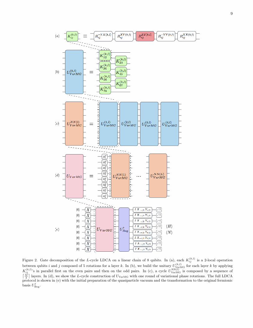
Figure 2. Gate decomposition of the L-cycle LDCA on a linear chain of 8 qubits. In (a), each K(k,l)ij is a 2-local operation

between qubits i and j composed of 5 rotations for a layer k. In (b), we build the unitary U(k,l)VarMG for each layer k by applying

K(k,l)ij ’s in parallel first on the even pairs and then on the odd pairs. In (c), a cycle U

NN(l)VarMG is composed by a sequence of⌈

M2

⌉layers. In (d), we show the L-cycle construction of UVarMG with one round of variational phase rotations. The full LDCA

protocol is shown in (e) with the initial preparation of the quasiparticle vacuum and the transformation to the original fermionicbasis U†

Bog.

10

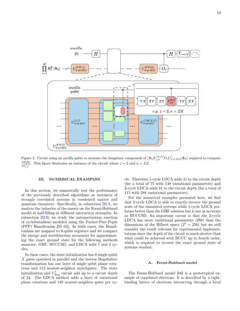
Figure 3. Circuit using an ancilla qubit to measure the imaginary component of 〈Φ0|V (k,l)†j,n OiU

′V arMG|Φ0〉 required to compute

∂E(Θ)

∂θ(k,l)j,n

. This figure illustrates an instance of the circuit where j = 2 and n = ZZ.

III. NUMERICAL EXAMPLES

In this section, we numerically test the performanceof the previously described algorithms on instances ofstrongly correlated systems in condensed matter andquantum chemistry. Specifically, in subsection IIIA, weanalyze the behavior of the ansatz on the Fermi-Hubbardmodel at half-filling at different interaction strengths. Insubsection III B, we study the automerization reactionof cyclobutadiene modeled using the Pariser-Parr-Pople(PPP) Hamiltonian [63–65]. In both cases, the Hamil-tonians are mapped to 8-qubit registers and we comparethe energy and wavefunction accuracies for approximat-ing the exact ground state for the following methodsansatzes: GHF, BUCCSD, and LDCA with 1 and 2 cy-cles.

In these cases, the state initialization has 8 single qubitX gates operated in parallel and the inverse Bogoliubovtransformation has one layer of single qubit phase rota-tions and 112 nearest-neighbor matchgates. The stateinitialization and U†Bog circuit add up to a circuit depthof 34. The LDCA method adds a layer of variationalphase rotations and 140 nearest-neighbor gates per cy-

cle. Therefore 1-cycle LDCA adds 41 to the circuit depth(for a total of 75 with 148 variational parameters) and2-cycle LDCA adds 81 to the circuit depth (for a total of115 with 288 variational parameters).

For the numerical examples presented here, we findthat 2-cycle LDCA is able to exactly recover the groundstate of the simulated systems while 1-cycle LDCA per-forms better than the GHF solution but is not as accurateas BUCCSD. An important caveat is that the 2-cycleLDCA has more variational parameters (288) than thedimensions of the Hilbert space (28 = 256) but we stillconsider the result relevant for experimental implemen-tations since the depth of the circuit is much shorter thanwhat could be achieved with BUCC up to fourth order,which is required to recover the exact ground state ofsystems studied.

A. Fermi-Hubbard model

The Fermi-Hubbard model [66] is a prototypical ex-ample of correlated electrons. It is described by a tight-binding lattice of electrons interacting through a local

11

Coulomb force. The Hamiltonian is given by

HFH = −t∑〈p,q〉

∑σ=↑,↓

(a†pσaqσ + a†qσapσ

)−µ∑p

∑σ=↑,↓

(npσ − 1

2

)+U

∑p

(np↑ − 1

2

) (np↓ − 1

2

),

(50)

where t is the kinetic energy between nearest-neighborsites 〈p, q〉, U is the static Coulomb interaction andµ is the chemical potential. The number operatoris npσ = a†pσaqσ. While the one-dimensional Fermi-Hubbard model can be solved exactly with the Betheansatz [67, 68], the two-dimensional version can only besolved exactly for very specific values of the parametersand a general solution remains elusive. The phase di-agram of the 2D model is known to be very rich andthere are strong arguments that a better understandingof the model could yield the key to explain the physicsof high-temperature cuprate superconductors [69–71].

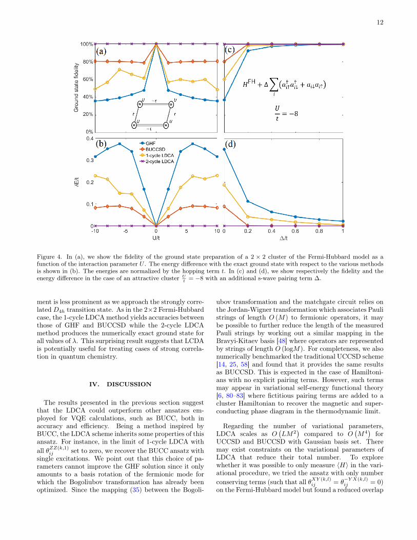
Hybrid quantum-classical methods to systematicallyapproximate the phase diagram of the Fermi-Hubbardmodel in the thermodynamical limit are known [6, 62] butthey require preparing the ground state of a large clusterof the model with an accuracy that cannot be reachedby previously proposed methods [5]. Here, we investi-gate the performance of the ansatz detailed in section IIon an example of a 2 × 2 cluster of the Fermi-Hubbardmodel at half-filling (µ = 0) that can be implemented ona 8-qubit quantum processor. As shown in figure 4, theGHF method performs well for small values of the inter-action strength U

t and exactly describes the tight-bindingcase where the Hamiltonian is quadratic. The BUCCSDansatz offers a significant improvement over the GHF so-lution but fails to reach the exact ground state at stronginteraction strengths. While 1-cycle LDCA offers an in-termediate solution between GHF and BUCCSD, the2-cycle LDCA solution performs surprisingly well as itis able to reach the exact ground state up to numeri-cal accuracy for all values of the interaction strength.In all cases the preparation fidelity |〈Ψ (Θ) |Ψ0〉|2 is di-rectly correlated with the energy difference δE betweenthe prepared state and the exact ground state |Ψ0〉. Wealso show that all methods are able to handle Hamil-tonians with pairing terms by introducing an artificial∆∑i

(a†i↑a

†i↓ + ai↓ai↑

). The accuracy of all methods im-

proves with increasing ∆t as the ground state gets closer

to a fermionic Gaussian state.We also tested a simpler one dimensional cluster of

the Fermi-Hubbard model with 2 sites and found that itwas possible to reach the exact ground state with bothBUCCSD and the 1-cycle LDCA method for all valuesof the parameter U . This is expected for the BUCCSDmethod as this is equivalent to a full configuration inter-action parametrization in this specific case. We do nothave sufficient information to determine the number ofcycles L required by LDCA to reach the ground stateas a function of the cluster size since it would require

much more intense numerics. However, the fact that a2× 1 cluster requires only 1 cycle and that the 2× 2 casereaches the ground state in 2 cycles leave open the pos-sibility that the scaling is not an exponential function ofthe cluster size.

B. Cyclobutadiene

As an example of a quantum chemistry application, westudied the accuracy of the proposed methods in the de-scription of cyclobutadiene automerization. The study ofthis reaction has been particularly challenging for theo-retical chemists due to the strongly correlated characterof the open-shell D4h transition state in contrast withthe weakly correlated character of the closed-shell D2h

ground state (1A1g) [72]. An accurate theoretical treat-ment of the transition state would allow to confirm sev-eral observations about the mechanism, such as the al-leged change in the aromatic character of the moleculebetween its ground and transition states as well as theinvolvement of a tunneling carbon atom in the reaction[72–75]. In addition, it would serve as a confirmation ofthe energy barrier for the automerization, for which ex-perimental reports vary between 1.6 and 12.0 kcal/mol[76].

Although the Hamiltonian for cyclobutadiene can beobtained from a Hartree-Fock or a Complete ActiveSpace (CAS) standard quantum chemistry calculation,we opted to describe the reaction using a Pariser-Parr-Pople (PPP) model Hamiltonian [63–65]. The PPPmodel captures the main physics of π-electron systemssuch as cyclobutadiene and also establishes a direct con-nection to the Fermi-Hubbard Hamiltonian studied in theprevious section. Using this model, the Hamiltonian ofcyclobutadiene can be written as

HPPP =∑i<j tijEij

+∑i Uiniαniβ + Vc

+ 12

∑ij γij(niα + niβ − 1)(njα + njβ − 1),

(51)where Eij =

∑σ=α,β a

†iσajσ + a†jσaiσ, niσ = a†iσaiσ,

and the variables γij are parameterized by the Mataga-Nishimoto formula [77]

γij(rij) =1

1/U + rij. (52)

The tij , U , and Vc parameters were obtained from [78, 79]as a function of the dimensionless reaction coordinate, λ,and the geometries of the ground as well as transitionstates were optimized at this level of theory.

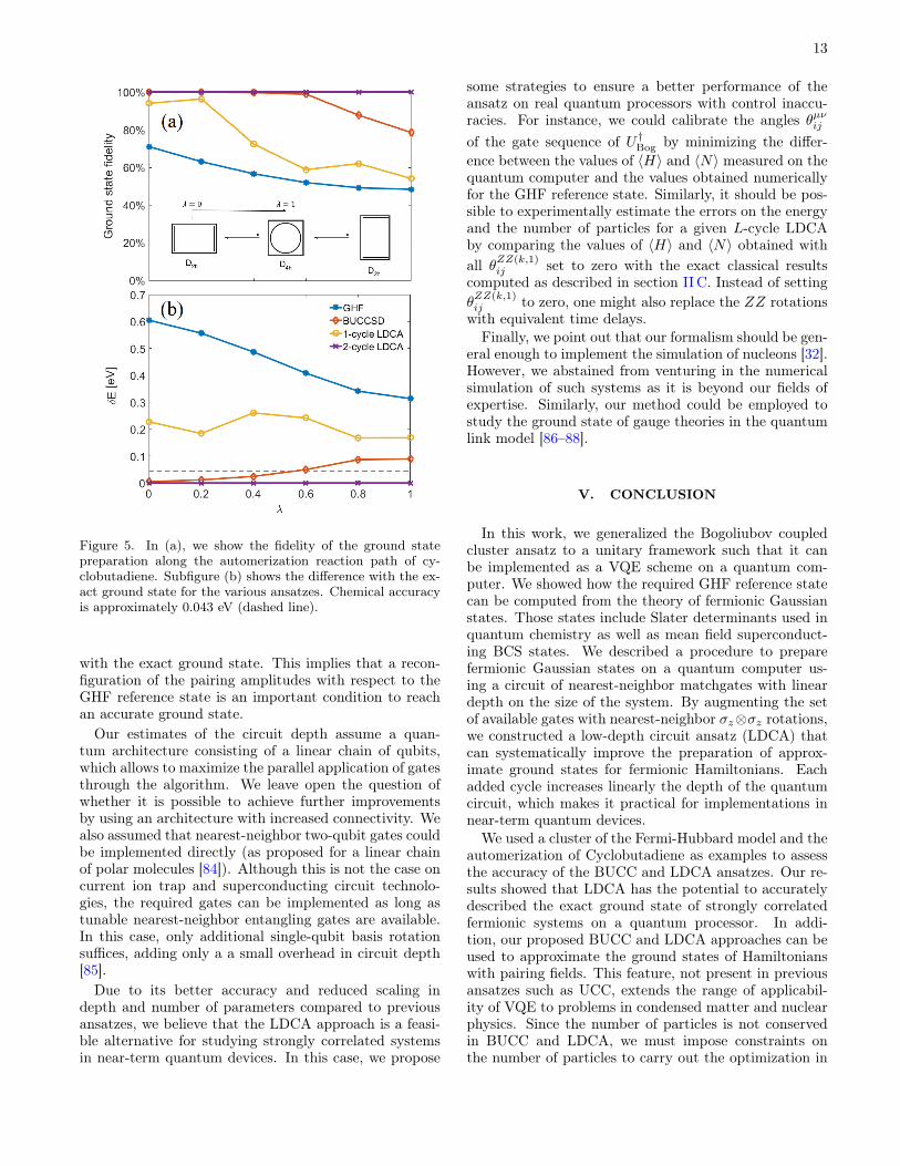
Figure 5 compares the accuracies of different ansatzesfor the cyclobutadiene automerization reaction. Weobserve that GHF ansatz is considerably improved byBUCCSD close to the D2h ground state but the improve-

12

Figure 4. In (a), we show the fidelity of the ground state preparation of a 2 × 2 cluster of the Fermi-Hubbard model as afunction of the interaction parameter U . The energy difference with the exact ground state with respect to the various methodsis shown in (b). The energies are normalized by the hopping term t. In (c) and (d), we show respectively the fidelity and theenergy difference in the case of an attractive cluster U

t= −8 with an additional s-wave pairing term ∆.

ment is less prominent as we approach the strongly corre-latedD4h transition state. As in the 2×2 Fermi-Hubbardcase, the 1-cycle LDCAmethod yields accuracies betweenthose of GHF and BUCCSD while the 2-cycle LDCAmethod produces the numerically exact ground state forall values of λ. This surprising result suggests that LCDAis potentially useful for treating cases of strong correla-tion in quantum chemistry.

IV. DISCUSSION

The results presented in the previous section suggestthat the LDCA could outperform other ansatzes em-ployed for VQE calculations, such as BUCC, both inaccuracy and efficiency. Being a method inspired byBUCC, the LDCA scheme inherits some properties of thisansatz. For instance, in the limit of 1-cycle LDCA withall θZZ(k,1)

ij set to zero, we recover the BUCC ansatz withsingle excitations. We point out that this choice of pa-rameters cannot improve the GHF solution since it onlyamounts to a basis rotation of the fermionic mode forwhich the Bogoliubov transformation has already beenoptimized. Since the mapping (35) between the Bogoli-

ubov transformation and the matchgate circuit relies onthe Jordan-Wigner transformation which associates Paulistrings of length O (M) to fermionic operators, it maybe possible to further reduce the length of the measuredPauli strings by working out a similar mapping in theBravyi-Kitaev basis [48] where operators are representedby strings of length O (logM). For completeness, we alsonumerically benchmarked the traditional UCCSD scheme[14, 25, 58] and found that it provides the same resultsas BUCCSD. This is expected in the case of Hamiltoni-ans with no explicit pairing terms. However, such termsmay appear in variational self-energy functional theory[6, 80–83] where fictitious pairing terms are added to acluster Hamiltonian to recover the magnetic and super-conducting phase diagram in the thermodynamic limit.

Regarding the number of variational parameters,LDCA scales as O

(LM2

)compared to O

(M4)

forUCCSD and BUCCSD with Gaussian basis set. Theremay exist constraints on the variational parameters ofLDCA that reduce their total number. To explorewhether it was possible to only measure 〈H〉 in the vari-ational procedure, we tried the ansatz with only numberconserving terms (such that all θXY (k,l)

ij = θ−Y X(k,l)ij = 0)

on the Fermi-Hubbard model but found a reduced overlap

13

Figure 5. In (a), we show the fidelity of the ground statepreparation along the automerization reaction path of cy-clobutadiene. Subfigure (b) shows the difference with the ex-act ground state for the various ansatzes. Chemical accuracyis approximately 0.043 eV (dashed line).

with the exact ground state. This implies that a recon-figuration of the pairing amplitudes with respect to theGHF reference state is an important condition to reachan accurate ground state.

Our estimates of the circuit depth assume a quan-tum architecture consisting of a linear chain of qubits,which allows to maximize the parallel application of gatesthrough the algorithm. We leave open the question ofwhether it is possible to achieve further improvementsby using an architecture with increased connectivity. Wealso assumed that nearest-neighbor two-qubit gates couldbe implemented directly (as proposed for a linear chainof polar molecules [84]). Although this is not the case oncurrent ion trap and superconducting circuit technolo-gies, the required gates can be implemented as long astunable nearest-neighbor entangling gates are available.In this case, only additional single-qubit basis rotationsuffices, adding only a a small overhead in circuit depth[85].

Due to its better accuracy and reduced scaling indepth and number of parameters compared to previousansatzes, we believe that the LDCA approach is a feasi-ble alternative for studying strongly correlated systemsin near-term quantum devices. In this case, we propose

some strategies to ensure a better performance of theansatz on real quantum processors with control inaccu-racies. For instance, we could calibrate the angles θµνijof the gate sequence of U†Bog by minimizing the differ-ence between the values of 〈H〉 and 〈N〉 measured on thequantum computer and the values obtained numericallyfor the GHF reference state. Similarly, it should be pos-sible to experimentally estimate the errors on the energyand the number of particles for a given L-cycle LDCAby comparing the values of 〈H〉 and 〈N〉 obtained withall θZZ(k,1)

ij set to zero with the exact classical resultscomputed as described in section IIC. Instead of settingθZZ(k,1)ij to zero, one might also replace the ZZ rotationswith equivalent time delays.

Finally, we point out that our formalism should be gen-eral enough to implement the simulation of nucleons [32].However, we abstained from venturing in the numericalsimulation of such systems as it is beyond our fields ofexpertise. Similarly, our method could be employed tostudy the ground state of gauge theories in the quantumlink model [86–88].

V. CONCLUSION

In this work, we generalized the Bogoliubov coupledcluster ansatz to a unitary framework such that it canbe implemented as a VQE scheme on a quantum com-puter. We showed how the required GHF reference statecan be computed from the theory of fermionic Gaussianstates. Those states include Slater determinants used inquantum chemistry as well as mean field superconduct-ing BCS states. We described a procedure to preparefermionic Gaussian states on a quantum computer us-ing a circuit of nearest-neighbor matchgates with lineardepth on the size of the system. By augmenting the setof available gates with nearest-neighbor σz⊗σz rotations,we constructed a low-depth circuit ansatz (LDCA) thatcan systematically improve the preparation of approx-imate ground states for fermionic Hamiltonians. Eachadded cycle increases linearly the depth of the quantumcircuit, which makes it practical for implementations innear-term quantum devices.

We used a cluster of the Fermi-Hubbard model and theautomerization of Cyclobutadiene as examples to assessthe accuracy of the BUCC and LDCA ansatzes. Our re-sults showed that LDCA has the potential to accuratelydescribed the exact ground state of strongly correlatedfermionic systems on a quantum processor. In addi-tion, our proposed BUCC and LDCA approaches can beused to approximate the ground states of Hamiltonianswith pairing fields. This feature, not present in previousansatzes such as UCC, extends the range of applicabil-ity of VQE to problems in condensed matter and nuclearphysics. Since the number of particles is not conservedin BUCC and LDCA, we must impose constraints onthe number of particles to carry out the optimization in

14

the classical computer. Future work will be devoted tobenchmarking the accuracy of the LDCA method for alarger variety of molecular systems and determining thescaling in the number of cycles required to describe theground states of general systems.

ACKNOWLEDGMENTS

We would like to thank Ryan Babbush for helpful dis-cussions. Jonathan Romero and Alán Aspuru-Guzik ac-knowledge the Air Force Office of Scientific Research forsupport under Award: FA9550-12-1-0046. Sukin Sim issupported by the DOE Computational Science GraduateFellowship under grant number DE-FG02-97ER25308.Pierre-Luc Dallaire Demers and Alán Aspuru-Guzik ac-knowledge support from the Vannevar Bush Fellowshipfrom the United States Department of Defense underaward number N00014-16-1-2008 under the Office ofNaval Research.

[1] R. P. Feynman, Int. J. Theor. Phys. 21, 467 (1982).[2] D. S. Abrams and S. Lloyd, Phys. Rev. Lett. 79, 2586

(1997).[3] M. Reiher, N. Wiebe, K. M. Svore, D. Wecker, and

M. Troyer, Proceedings of the National Academy of Sci-ences 114, 7555 (2017).

[4] B. Bauer, D. Wecker, A. J. Millis, M. B. Hastings,and M. Troyer, Phys. Rev. X 6 (2016), 10.1103/phys-revx.6.031045.

[5] D. Wecker, M. B. Hastings, N. Wiebe, B. K. Clark,C. Nayak, and M. Troyer, Phys. Rev. A 92, 062318(2015).

[6] P.-L. Dallaire-Demers and F. K. Wilhelm, Phys. Rev. A93, 032303 (2016).

[7] G. Ortiz, J. E. Gubernatis, E. Knill, and R. Laflamme,Physical Review A 64 (2001), 10.1103/phys-reva.64.022319.

[8] A. Aspuru-Guzik, Science 309, 1704 (2005).[9] I. Kassal, S. P. Jordan, P. J. Love, M. Mohseni, and

A. Aspuru-Guzik, Proceedings of the National Academyof Sciences 105, 18681 (2008).

[10] J. D. Whitfield, J. Biamonte, and A. Aspuru-Guzik,Molecular Physics 109, 735 (2011).

[11] I. Kassal, J. D. Whitfield, A. Perdomo-Ortiz, M.-H.Yung, and A. Aspuru-Guzik, Annu. Rev. Phys. Chem.62, 185 (2011).

[12] L. Veis, J. Višňák, T. Fleig, S. Knecht, T. Saue, L. Viss-cher, and J. Pittner, Physical Review A 85 (2012),10.1103/physreva.85.030304.

[13] U. L. Heras, A. Mezzacapo, L. Lamata, S. Filipp,A. Wallraff, and E. Solano, Phys. Rev. Lett. 112, 200501(2013).

[14] A. Peruzzo, J. McClean, P. Shadbolt, M.-H. Yung, X.-Q.Zhou, P. J. Love, A. Aspuru-Guzik, and J. L. O’Brien,Nat. Commun. 5, 4213 (2014).

[15] R. Barends, L. Lamata, J. Kelly, L. Garcia-Alvarez, A. G.Fowler, A. Megrant, E. Jeffrey, T. C. White, D. Sank,J. Y. Mutus, B. Campbell, Y. Chen, Z. Chen, B. Chiaro,A. Dunsworth, I.-C. Hoi, C. Neill, P. J. J. O’Malley,C. Quintana, P. Roushan, A. Vainsencher, J. Wenner,E. Solano, and J. M. Martinis, Nat. Commun. 6, 7654(2015).

[16] U. L. Heras, L. Garcia-Alvarez, A. Mezzacapo, E. Solano,and L. Lamata, EPJ Quantum Technology 2, 8 (2015).

[17] P. J. J. O’Malley, R. Babbush, I. D. Kivlichan,

J. Romero, J. R. McClean, R. Barends, J. Kelly,P. Roushan, A. Tranter, N. Ding, B. Campbell, Y. Chen,Z. Chen, B. Chiaro, A. Dunsworth, A. G. Fowler, E. Jef-frey, A. Megrant, J. Y. Mutus, C. Neill, C. Quintana,D. Sank, A. Vainsencher, J. Wenner, T. C. White, P. V.Coveney, P. J. Love, H. Neven, A. Aspuru-Guzik, andJ. M. Martinis, Phys. Rev. X 6 (2016), 10.1103/phys-revx.6.031007.

[18] D. Poulin, M. B. Hastings, D. Wecker, N. Wiebe, A. C.Doherty, and M. Troyer, QIC 15, 361 (2015).

[19] R. Babbush, D. W. Berry, I. D. Kivlichan, A. Y. Wei,P. J. Love, and A. Aspuru-Guzik, New J. Phys. 18,033032 (2016).

[20] G. Zhu, Y. Subasi, J. D. Whitfield, and M. Hafezi,(2017), 1707.04760v1.

[21] T. Monz, D. Nigg, E. A. Martinez, M. F. Brandl,P. Schindler, R. Rines, S. X. Wang, I. L. Chuang, andR. Blatt, Science 351, 1068 (2016).

[22] N. M. Linke, D. Maslov, M. Roetteler, S. Debnath,C. Figgatt, K. A. Landsman, K. Wright, and C. Mon-roe, Proceedings of the National Academy of Sciences114, 3305 (2017).

[23] C. Neill, P. Roushan, K. Kechedzhi, S. Boixo, S. V.Isakov, V. Smelyanskiy, R. Barends, B. Burkett,Y. Chen, Z. Chen, B. Chiaro, A. Dunsworth, A. Fowler,B. Foxen, R. Graff, E. Jeffrey, J. Kelly, E. Lucero,A. Megrant, J. Mutus, M. Neeley, C. Quintana, D. Sank,A. Vainsencher, J. Wenner, T. C. White, H. Neven, andJ. M. Martinis, (2017), 1709.06678v1.

[24] D. Wecker, M. B. Hastings, and M. Troyer, “Towardspractical quantum variational algorithms,” (2015).

[25] J. R. McClean, J. Romero, R. Babbush, and A. Aspuru-Guzik, New Journal of Physics 18, 023023 (2016).

[26] K. Temme, S. Bravyi, and J. M. Gambetta, (2017),1612.02058v2.

[27] Y. Li and S. C. Benjamin, Physical Review X 7 (2017),10.1103/physrevx.7.021050.

[28] A. Kandala, A. Mezzacapo, K. Temme, M. Takita,M. Brink, J. M. Chow, and J. M. Gambetta, Nature549, 242 (2017).

[29] R. Babbush, N. Wiebe, J. McClean, J. McClain,H. Neven, and G. K.-L. Chan, (2017), 1706.00023v2.

[30] L. Z. Stolarczyk and H. J. Monkhorst, Mol. Phys. 108,3067 (2010).

[31] Z. Rolik and M. Kállay, The Journal of Chemical Physics

15

141, 134112 (2014).[32] A. Signoracci, T. Duguet, G. Hagen, and

G. R. Jansen, Physical Review C 91 (2015),https://doi.org/10.1103/PhysRevC.91.064320.

[33] N. S. O. Attila Szabo, Modern Quantum Chemistry(Dover Publications Inc., 1996).

[34] G. Rickayzen, Green’s Functions and Condensed Matter(Academic Press, 1991).

[35] D. Senechal, A.-M. Tremblay, and C. Bourbonnais, The-oretical Methods for Strongly Correlated Electrons, CRMSeries in Mathematical Physics (Springer-Verlag NewYork, 2004).

[36] A. J. Leggett, Quantum Liquids (Oxford UniversityPress, 2006).

[37] P. Ring and P. Schuck, The nuclear many-body problem(Springer-Verlag GmbH, 1980).

[38] M. Bender, P.-H. Heenen, and P.-G. Reinhard, Reviewsof Modern Physics 75, 121 (2003).

[39] B. Loiseau and Y. Nogami, Nucl. Phys. B 2, 470 (1967).[40] C. V. Kraus, M. M. Wolf, J. I. Cirac,

and G. Giedke, Phys. Rev. A 79 (2009),https://doi.org/10.1103/PhysRevA.79.012306.

[41] C. V. Kraus and J. I. Cirac, New J. Phys. 12, 113004(2010).

[42] L. N. Cooper, Physical Review 104, 1189 (1956).[43] J. Bardeen, L. N. Cooper, and J. R. Schrieffer, Physical

Review 106, 162 (1957).[44] F. Verstraete, J. I. Cirac, and J. I. Latorre, Phys. Rev.

A 79, 032316 (2009).[45] C. Bloch and A. Messiah, Nuclear Physics 39, 95 (1962).[46] L. G. Valiant, SIAM Journal on Computing 31, 1229

(2002).[47] B. M. Terhal and D. P. DiVincenzo, Phys. Rev. A 65,

032325 (2002).[48] S. B. Bravyi and A. Y. Kitaev, Annals of Physics 298,

210 (2002).[49] R. Jozsa and A. Miyake, Proc. R. Soc. A 464, 3089

(2008).[50] D. J. Brod, Phys. Rev. A 93, 062332 (2016).[51] Z. Jiang, K. J. Sung, K. Kechedzhi, V. N. Smelyanskiy,

and S. Boixo, arXiv preprint arXiv:1711.05395 (2017).[52] D. K. Hoffman, R. C. Raffenetti, and K. Ruedenberg,

Journal of Mathematical Physics 13, 528 (1972).[53] N. Khaneja, T. Reiss, C. Kehlet, T. Schulte-Herbr?ggen,

and S. J. Glaser, Journal of Magnetic Resonance 172,296 (2005).

[54] S. Machnes, U. Sander, S. J. Glaser, P. de Fouquières,A. Gruslys, S. Schirmer, and T. Schulte-Herbr?ggen,Physical Review A 84 (2011), 10.1103/Phys-RevA.84.022305.

[55] P. Jordan and E. Wigner, Z. Phys. 47, 631 (1928).[56] J. T. Seeley, M. J. Richard, and P. J. Love, J. Chem.

Phys. 137, 224109 (2012).[57] M. B. Hastings, D. Wecker, B. Bauer, and M. Troyer,

Quantum Info. Comput. 15 (2015).[58] J. Romero, R. Babbush, J. R. McClean, C. Hempel,

P. Love, and A. Aspuru-Guzik, (2017), 1701.02691v1.[59] T. Shi, E. Demler, and J. I. Cirac, (2017), 1707.05902v1.[60] T. G. Kolda, R. M. Lewis, and V. Torczon, SIAM Rev.

45, 385 (2006).[61] J. R. McClean, R. Babbush, P. J. Love, and A. Aspuru-

Guzik, Journal of Physical Chemistry Letters 5, 4368(2014).

[62] P.-L. Dallaire-Demers and F. K. Wilhelm, Physical Re-view A 94 (2016), 10.1103/physreva.94.062304.

[63] R. Pariser and R. G. Parr, The Journal of ChemicalPhysics 21, 466 (1953).

[64] R. Pariser and R. G. Parr, The Journal of ChemicalPhysics 21, 767 (1953).

[65] J. A. Pople, Transactions of the Faraday Society 49, 1375(1953).

[66] J. Hubbard, Proceedings of the Royal Society of London.Series A, Mathematical and Physical Sciences 276, 238(1963).

[67] E. H. Lieb and F. Y. Wu, Physica A 321, 1 (2003).[68] F. Essler, H. Frahm, F. Gohmann, A. Klumper, and

V. E. Korepin, The One-Dimensional Hubbard Model(Cambridge University Press, 2005).

[69] P. W. Anderson, Science 235, 1196 (1987).[70] A. J. Leggett, Proc. Natl. Acad. Sci. USA 96, 8365

(1999).[71] P. W. Anderson, P. A. Lee, M. Randeria, T. M. Rice,

N. Trivedi, and F. C. Zhang, J Phys. Condens. Matter16, R755 (2004).

[72] P. G. Szalay, T. M?ller, G. Gidofalvi, H. Lischka, andR. Shepard, Chemical Reviews 112, 108 (2012).

[73] B. R. Arnold and J. Michl, Kinetics and Spectroscopy ofCarbenes and Biradicals (Springer Us, 2013).

[74] B. R. Arnold, J. G. Radziszewski, A. Campion, S. S.Perry, and J. Michl, Journal of the American ChemicalSociety 113, 692 (1991).

[75] B. R. Arnold and J. Michl, The Journal of PhysicalChemistry 97, 13348 (1993).

[76] D. W. Whitman and B. K. Carpenter, Journal of theAmerican Chemical Society 104, 6473 (1982).

[77] N. Mataga and K. Nishimoto, Z. phys. Chem 13, 140(1957).

[78] T. G. Schmalz, L. Serrano-Andrés, V. Sauri, M. Merchán,and J. M. Oliva, The Journal of Chemical Physics 135,194103 (2011).

[79] T. G. Schmalz, Croatica Chemica Acta 86, 419 (2013).[80] M. Potthoff, M. Aichhorn, and C. Dahnken, Phys. Rev.

Lett. 91, 206402 (2003).[81] M. Potthoff, Condens. Mat. Phys. 9, 557 (2006).[82] D. Senechal, “An introduction to quantum cluster meth-

ods,” (2008), arXiv:cond-mat.str-el/0806.2690v2 [cond-mat.str-el].

[83] D. Senechal, in High Performance Computing Systemsand Applications (2008).

[84] F. Herrera, Y. Cao, S. Kais, and K. B. Whaley, NewJournal of Physics 16, 075001 (2014).

[85] M. A. Nielsen and I. L. Chuang, Quantum Computationand Quantum Information (Cambridge University Press,2001).

[86] T. Byrnes and Y. Yamamoto, Phys. Rev. A 73 (2006),https://doi.org/10.1103/PhysRevA.73.022328.

[87] E. Zohar and M. Burrello, Phys. Rev. D 91, 054506(2015).

[88] M. Dalmonte and S. Montangero, Contemporary Physics57, 388 (2016).