WRF Physics Options

Acknowledgements:

Slides by Jimy Dudhia (NCAR)

Dr Meral DemirtaşDr Meral DemirtaşTurkish State Meteorological ServiceTurkish State Meteorological Service

Weather Forecasting DepartmentWeather Forecasting Department

WMO, Training Course, 26-30 September 2011WMO, Training Course, 26-30 September 2011Alanya, TurkeyAlanya, Turkey

WRF Physics

• Radiation– Longwave (ra_lw_physics)– Shortwave (ra_sw_physics)

• Surface– Surface layer (sf_sfclay_physics)– Land/water surface (sf_surface_physics)

• PBL (bl_physics)• Cumulus parameterization (cu_physics)• Microphysics (mp_physics)• Turbulence/Diffusion (diff_opt, km_opt)

Radiation

Atmospheric temperature tendency

Surface radiative fluxes

Radiation physics options

• Long-wave radiation options: 6

• Short-wave radiation options: 6

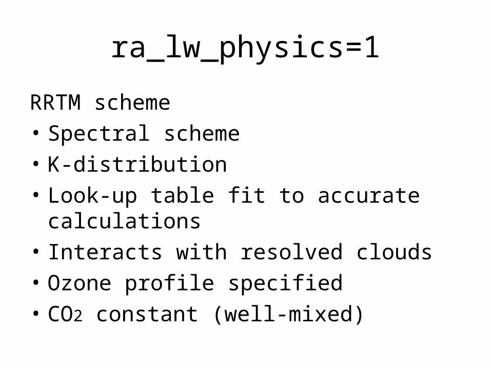
ra_lw_physics=1

RRTM scheme

• Spectral scheme

• K-distribution

• Look-up table fit to accurate calculations

• Interacts with resolved clouds

• Ozone profile specified

• CO2 constant (well-mixed)

ra_lw_physics=3

• CAM3 scheme • Spectral scheme • 8 longwave bands • Look-up table fit to accurate calculations • Interacts with cloud fractions • Can interact with trace gases and aerosols • Ozone profile function of month, latitude • CO2 changes based on year (since V3.1) • Top-of-atmosphere (TOA) and surface

diagnostics for climate ARW only

ra_lw_physics=4

RRTMG longwave scheme (Since V3.1) • Spectral scheme 16 longwave bands (K-distribution) • Look-up table fit to accurate calculations • Interacts with cloud fractions (MCICA, Monte

Carlo Independent Cloud Approximation random overlap method)

• Ozone profile specified • CO2 and trace gases specified • WRF-Chem optical depth • TOA and surface diagnostics for climate

ARW only

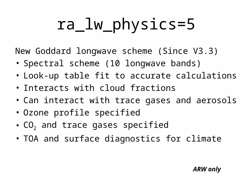
ra_lw_physics=5

New Goddard longwave scheme (Since V3.3) • Spectral scheme (10 longwave bands) • Look-up table fit to accurate calculations • Interacts with cloud fractions • Can interact with trace gases and aerosols • Ozone profile specified

• CO2 and trace gases specified

• TOA and surface diagnostics for climate

ARW only

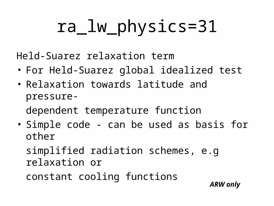
ra_lw_physics=31

Held-Suarez relaxation term • For Held-Suarez global idealized test • Relaxation towards latitude and pressure-

dependent temperature function • Simple code - can be used as basis for other

simplified radiation schemes, e.g relaxation or

constant cooling functions

ARW only

ra_lw_physics=99

GFDL longwave scheme • used in Eta/NMM • Default code is used with Ferrier microphysics

– Remove #define to compile for use without Ferrier

• Spectral scheme from global model • Also uses tables • Interacts with clouds (cloud fraction) • Ozone profile based on season, latitude • CO2 fixed • ra_lw_physics=98 (nearly identical) for HWRF

ra_sw_physics=1

MM5 shortwave (Dudhia)• Simple downward calculation • Clear-sky scattering

– swrad_scat tuning parameter • 1.0 = 10% scattered, 0.5=5%, etc.

– WRF-Chem aerosol effect (PM2.5)

• Water vapor absorption • Cloud albedo and absorption • No ozone effect (model top below 50 hPa OK)

ARW only

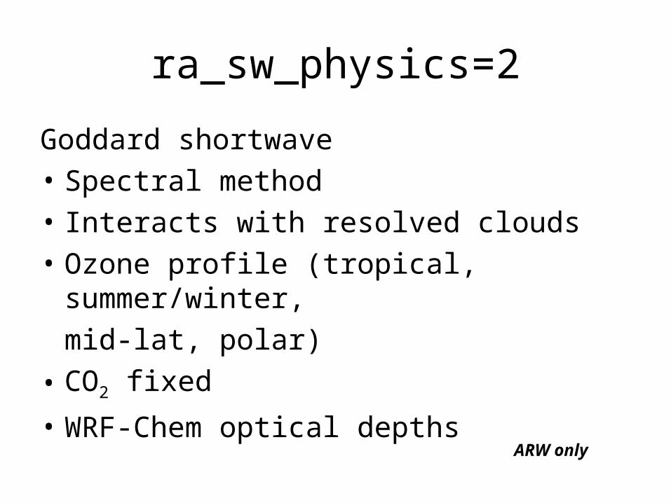
ra_sw_physics=2

Goddard shortwave

• Spectral method

• Interacts with resolved clouds

• Ozone profile (tropical, summer/winter,

mid-lat, polar)

• CO2 fixed

• WRF-Chem optical depths ARW only

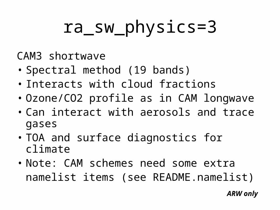
ra_sw_physics=3

CAM3 shortwave • Spectral method (19 bands) • Interacts with cloud fractions • Ozone/CO2 profile as in CAM longwave • Can interact with aerosols and trace gases • TOA and surface diagnostics for climate • Note: CAM schemes need some extra

namelist items (see README.namelist)

ARW only

ra_sw_physics=4

RRTMG shortwave (Since V3.1) • Spectral method (14 bands) • Interacts with cloud fractions (MCICA

method) • Ozone/CO2 profile as in RRTMG longwave • Trace gases specified • WRF-Chem optical depths • TOA and surface diagnostics for climate

ARW only

ra_sw_physics=5

New Goddard shortwave scheme(Since V3.3)

• Spectral scheme (11 shortwave bands) • Look-up table fit to accurate calculations • Interacts with cloud fractions • Ozone profile specified • CO2 and trace gases specified • TOA and surface diagnostics for climate

ARW only

ra_sw_physics=99

GFDL shortwave

• Used in Eta/NMM model

• Default code is used with Ferrier microphysics (see GFDL longwave)

• Ozone/CO2 profile as in GFDL longwave

• Interacts with clouds (and cloud fraction)

• ra_lw_physics=98 (nearly identical) for HWRF

Slope effects on shortwave

• In V3.2 available for all shortwave options • Represents effect of slope on surface solar

flux accounting for diffuse/direct effects • slope_rad=1: activates slope effects - may be

useful for complex topography and grid

lengths < 2 km. • topo_shading=1: shading of neighboring grids by

mountains - may be useful for grid lengths < 1 km.

nrads/nradl

Radiation time-step recommendation– Number of fundamental steps per radiation

call– Operational setting should be 3600/dt– Higher resolution could be used, e.g. 1800/dt– Use nrads=nradl in NMM

NMM only

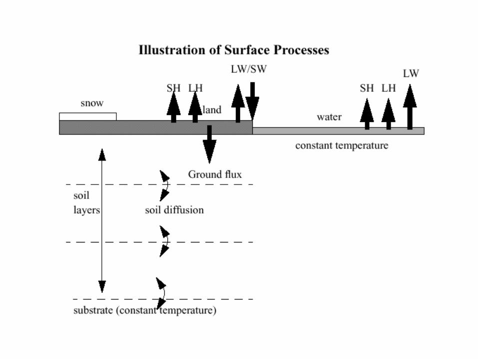
Surface schemes

Surface layer of atmosphere diagnostics (exchange coeffs)

Land Surface: Soil temperature, moisture, snow prediction, sea-ice temperature

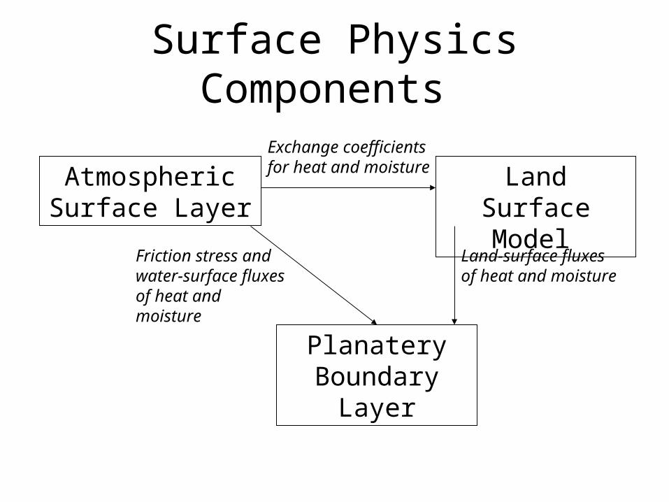
Surface Physics Components

Atmospheric Surface Layer

Land Surface Model

Planatery Boundary Layer

Exchange coefficients for heat and moisture

Land-surface fluxes of heat and moisture

Friction stress and water-surface fluxes of heat and moisture

Surface Fluxes

• Heat, moisture and momentum

H=ρcpu*θ* E=ρu*q*

where

Subscript r is reference level (lowest model level, or 2 m or 10 m) z0 are the roughness lengths.

Roughness Lengths

• Roughness lengths are a measure of the “initial”

length scale of surface eddies, and generally differ for velocity and scalars.

• Roughness length depends on land-use type • Some schemes use smaller roughness length

for heat than for momentum. • For water points roughness length is a function

of surface wind speed.

Exchange Coefficient

• Chs is the exchange coefficient for heat, defined such that

H=ρcp ChsΔθ

It is related to the roughness length and u* by

Surface scheme options

• Surface layer scheme options: 6

• Surface physics options: 3

• Surface urban physics options: 3

sf_sfclay_physics=1

Monin-Obukhov similarity theory• Taken from standard relations used in MM5

MRF PBL• Provides exchange coefficients to surface (land)

scheme• iz0tlnd thermal roughness length options for land

points (0: Original Carlson-Boland, 1: Chen-Zhang) – Chen and Zhang (2009, JGR) modifies Zilitinkevich

method with vegetation height • Should be used with bl_pbl_physics=1 or 99

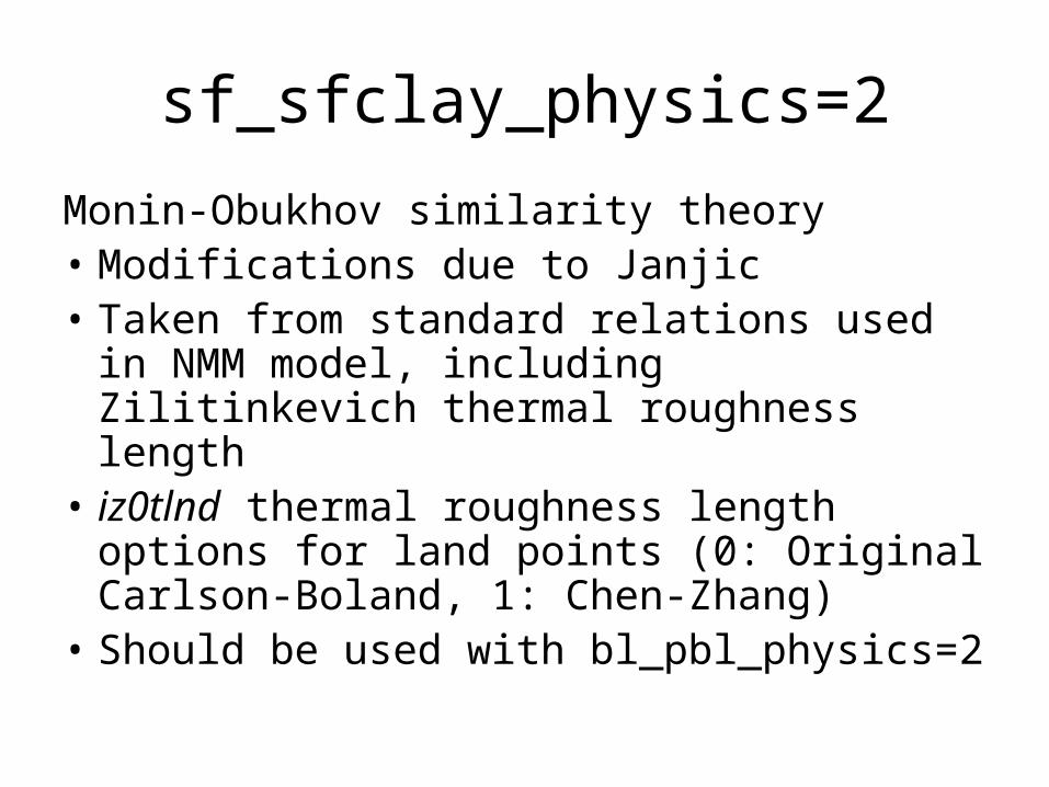
sf_sfclay_physics=2

Monin-Obukhov similarity theory• Modifications due to Janjic• Taken from standard relations used in

NMM model, including Zilitinkevich thermal roughness length

• iz0tlnd thermal roughness length options for land points (0: Original Carlson-Boland, 1: Chen-Zhang)

• Should be used with bl_pbl_physics=2

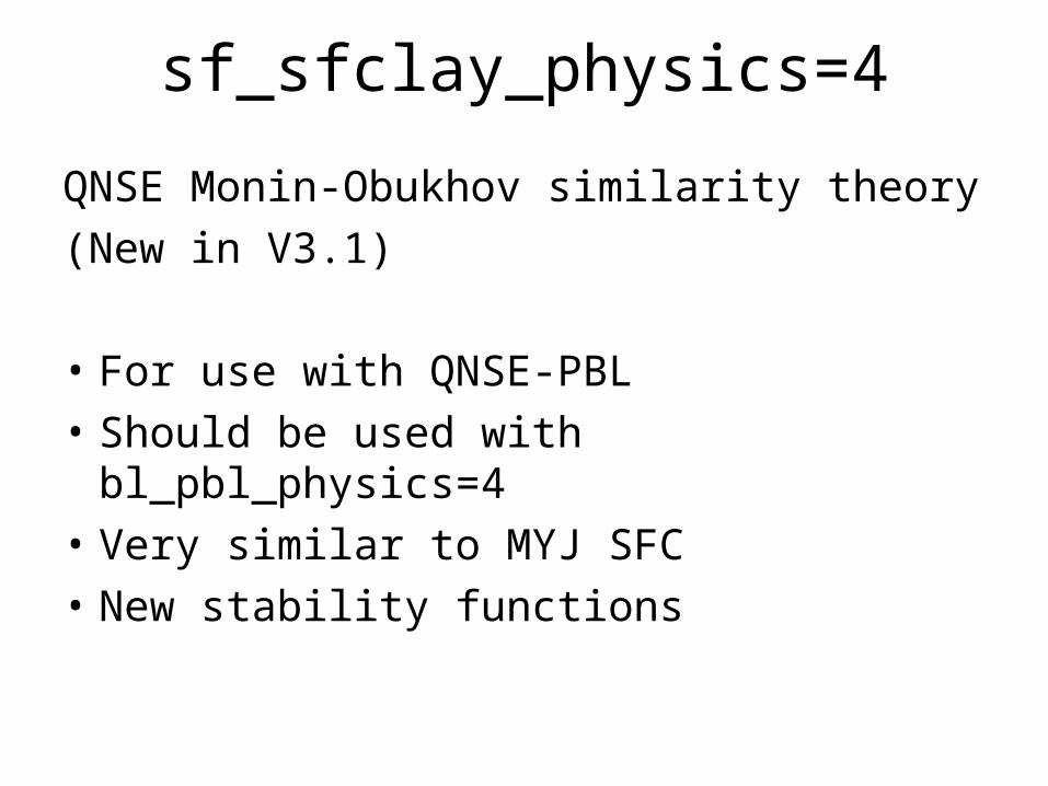
sf_sfclay_physics=4

QNSE Monin-Obukhov similarity theory

(New in V3.1)

• For use with QNSE-PBL

• Should be used with bl_pbl_physics=4

• Very similar to MYJ SFC

• New stability functions

sf_sfclay_physics=5

MYNN Monin-Obukhov similarity theory

(New in V3.1)

• For use with MYNN-PBL

• Should be used with bl_pbl_physics=5

ARW only

sf_sfclay_physics=7

Pleim-Xiu surface layer (EPA)

(New in Version 3 )

• For use with PX LSM and ACM PBL – Should be used with sf_surface_physics=7

and bl_pbl_physics=7

ARW only

sf_sfclay_physics=10

TEMF surface layer (Angevine et al.)

(New in Version 3.3 )

• For use with TEMF PBL – Should be used with bl_pbl_physics=10

ARW only

sf_surface_physics=1

5-layer thermal diffusion model from MM5

• Predict ground temp and soil temps

• Thermal properties depend on land use

• No soil moisture or snow-cover prediction

• Moisture availability based on land-use only

• Provides heat and moisture fluxes for PBL

ARW only

sf_surface_physics=8

RUC Land Surface Model (Smirnova)

• Vegetation effects included

• Predicts soil temperature and soil moisture in six layers

• Multi-layer snow model

• Provides heat and moisture fluxes for PBL

VEGPARM.TBL Text (ASCII) file that has vegetation properties for Noah and RUC LSMs (separate sections in this table)

• 24 USGS categories or 20 MODIS categories (new) from 30” global dataset

• Each type is assigned min/max value of – Albedo – Leaf Area Index – Emissivity – Roughness length

• Other vegetation properties (stomatal resistance etc.) • From 3.1, monthly vegetation fraction determines seasonal

cycle between min and max values in Noah • There is also a SOILPARM.TBL for soil properties in Noah and

RUC

LANDUSE.TBLText (ASCII) file that has land-use properties for 5-layer slab model

(vegetation, urban, water, etc.)

• From Version 3.1 Noah LSM does not use this table 24 USGS categories or 20 MODIS categories (new) from 30” global dataset

• Each type is assigned summer/winter value – Albedo – Emissivity – Roughness length

• Other table properties (thermal inertia, moisture availability, snow albedo effect) are used by 5-layer model

• Also note – Other tables (VEGPARM.TBL, etc.) are used by Noah – RUC LSM uses same table files after Version 3

Initializing LSMs (1)• Noah and RUC LSM require additional fields for

initialization• Soil temperature• Soil moisture• Snow liquid equivalent

• These are in the Grib files, but are not from observations

• They come from “offline” models driven by

observations (rainfall, radiation, surface temperature, humidity wind)

Initializing LSMs (2)• There are consistent model-derived datasets for Noah and RUC

LSMs

– Eta/GFS/AGRMET/NNRP for Noah (although some have limited soil levels available)

– RUC for RUC

• But, resolution of mesoscale land-use means there will be inconsistency in elevation, soil type and vegetation

• This leads to spin-up as adjustments occur in soil temperature and moisture

• This spin-up can only be avoided by running offline model on the same grid (e.g. HRLDAS for Noah)

• Cycling land state between forecasts also helps, but may propagate errors (e.g in rainfall effect on soil moisture)

Planetary Boundary Layer

Boundary layer fluxes (heat, moisture, momentum)

Vertical diffusion

PBL options

• Planatery boundary layer options: 10

bl_pbl_physics=1

YSU PBL scheme (Hong, Noh and Dudhia 2006)

• Parabolic K profile mixing in dry convective boundary layer

• Troen-Mahrt countergradient flux (non-local) • Depth of PBL determined from thermal profile • Explicit treatment of entrainment • Vertical diffusion depends on Ri in free

atmosphere • New stable surface BL mixing using bulk Ri

bl_pbl_physics=2

Mellor-Yamada-Janjic (Eta/NMM) PBL

• 1.5-order, level 2.5, TKE prediction

• Local-K vertical mixing in boundary layer and free atmosphere

• TKE_MYJ is advected by NMM, not by

ARW (yet)

bl_pbl_physics=4

QNSE (Quasi-Normal Scale Elimination) PBL from Galperin and Sukoriansky • 1.5-order, level 2.5, TKE prediction • Local TKE-based vertical mixing in

boundary layer and free atmosphere • New theory for stably stratified case • Mixing length follows MYJ, TKE

production simplified from MYJ

bl_pbl_physics=5 and 6

MYNN (Nakanishi and Niino) PBL • (5)1.5-order, level 2.5, TKE prediction, OR • (6)2nd-order, level 3, TKE, θ’2,q’2 and θ’q’

prediction • Local TKE-based vertical mixing in boundary • layer and free atmosphere • Since V3.1 • TKE advected since V3.3 (output name: QKE)

bl_pbl_physics=7

Asymmetrical Convective Model, Version 2

(ACM2) PBL (Pleim and Chang)

• Blackadar-type thermal mixing upwards

from surface layer • Local mixing downwards • PBL height from critical bulk Richardson

number

ARW only

bl_pbl_physics=8

BouLac PBL (Bougeault and Lacarrère)

(Since V3.1)

• TKE prediction scheme • Designed to work with multi-layer urban model

(BEP)

ARW only

bl_pbl_physics=9

CAM UW PBL (Bretherton and Park, U. Washington)

(New in V3.3)

• TKE prediction scheme • From current CESM climate model

physics • Use with sf_sfclay_physics=2

ARW only

bl_pbl_physics=10

Total Energy - Mass Flux (TEMF) PBL (Angevine et al.) (New in V3.3)

• Total Turbulent Energy (kinetic + potential) prediction scheme

• Includes mass-flux shallow convection

ARW only

bl_pbl_physics=99

MRF PBL scheme (Hong and Pan 1996)

• Non-local-K mixing in dry convective boundary layer

• Depth of PBL determined from critical Ri number

• Vertical diffusion depends on Ri in free atmosphere

ARW only

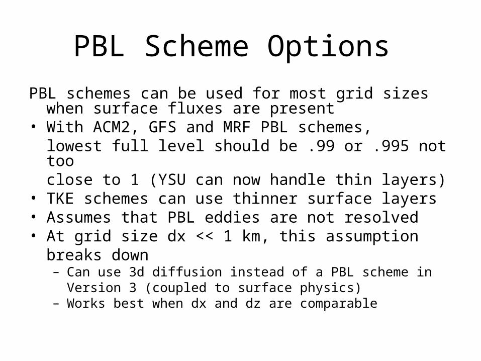
PBL Scheme Options

PBL schemes can be used for most grid sizes when surface fluxes are present

• With ACM2, GFS and MRF PBL schemes, lowest full level should be .99 or .995 not too close to 1 (YSU can now handle thin layers)

• TKE schemes can use thinner surface layers • Assumes that PBL eddies are not resolved • At grid size dx << 1 km, this assumption

breaks down – Can use 3d diffusion instead of a PBL scheme in

Version 3 (coupled to surface physics) – Works best when dx and dz are comparable

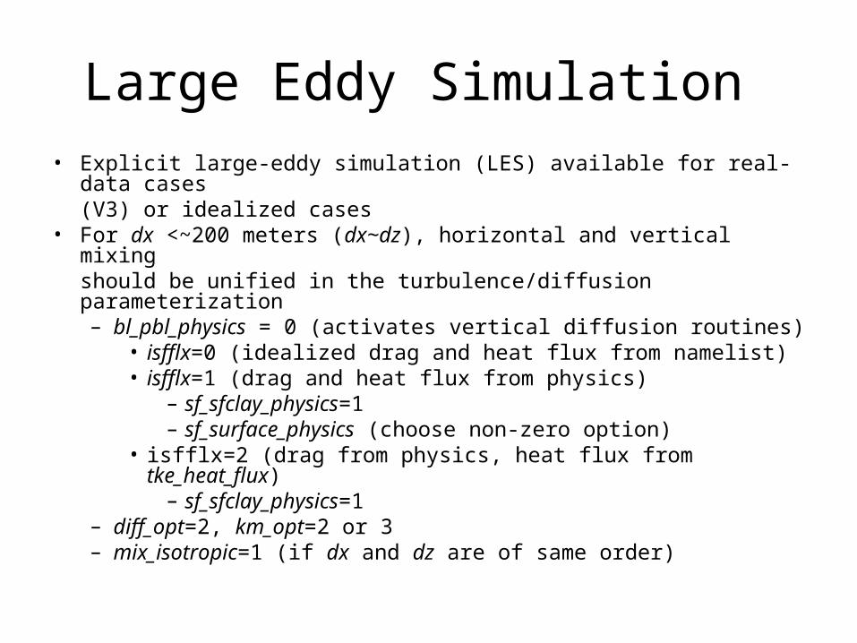
Large Eddy Simulation • Explicit large-eddy simulation (LES) available for real-data cases

(V3) or idealized cases • For dx <~200 meters (dx~dz), horizontal and vertical mixing

should be unified in the turbulence/diffusion parameterization – bl_pbl_physics = 0 (activates vertical diffusion routines)

• isfflx=0 (idealized drag and heat flux from namelist) • isfflx=1 (drag and heat flux from physics)

– sf_sfclay_physics=1 – sf_surface_physics (choose non-zero option)

• isfflx=2 (drag from physics, heat flux from tke_heat_flux) – sf_sfclay_physics=1

– diff_opt=2, km_opt=2 or 3 – mix_isotropic=1 (if dx and dz are of same order)

Gravity Wave Drag

(gwd_opt=1 for ARW, 2 for NMM)

• ARW scheme from Hong et al. (New in V3.1) • Accounts for orographic gravity wave effect

on momentum profile • Extra sub-grid orographic information comes

from geogrid (of WPS)• Probably needed only if all below apply

dx > 10 km • Simulations longer than 5 days • Domains including mountains

Cumulus Parameterization

Atmospheric heat and moisture

cloud tendencies

Surface rainfall

Cumulus scheme options

• Cumulus parameterization options: 8

cu_physics=1

New Kain-Fritsch • As in MM5 and Eta/NMM ensemble version • Includes shallow convection (no downdrafts) • Low-level vertical motion in trigger function • CAPE removal time scale closure • Mass flux type with updrafts and downdrafts, entrainment and

detrainment • Includes cloud, rain, ice, snow detrainment • Clouds persist over convective time scale

(recalculated every convective step in NMM) • Old KF is option 99

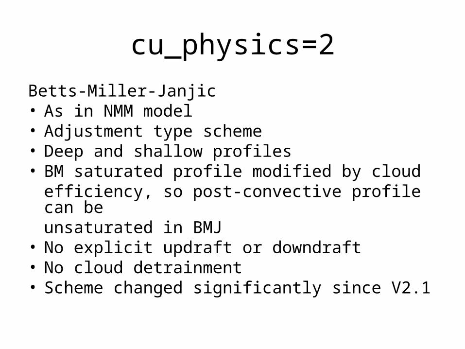
cu_physics=2

Betts-Miller-Janjic• As in NMM model• Adjustment type scheme• Deep and shallow profiles • BM saturated profile modified by cloud

efficiency, so post-convective profile can be unsaturated in BMJ

• No explicit updraft or downdraft • No cloud detrainment • Scheme changed significantly since V2.1

cu_physics=3

Grell-Devenyi Ensemble

• Multiple-closure (CAPE removal, quasi-

equilibrium, moisture convergence, cloud-

base ascent) - 16 mass flux closures • Multi-parameter (maximum cap, precipitation efficiency) -

e.g. 3 cap strengths, 3 efficiencies • Explicit updrafts/downdrafts • Includes cloud and ice detrainment • Mean feedback of ensemble is applied • Weights can be tuned (spatially, temporally)

to optimize scheme (training)

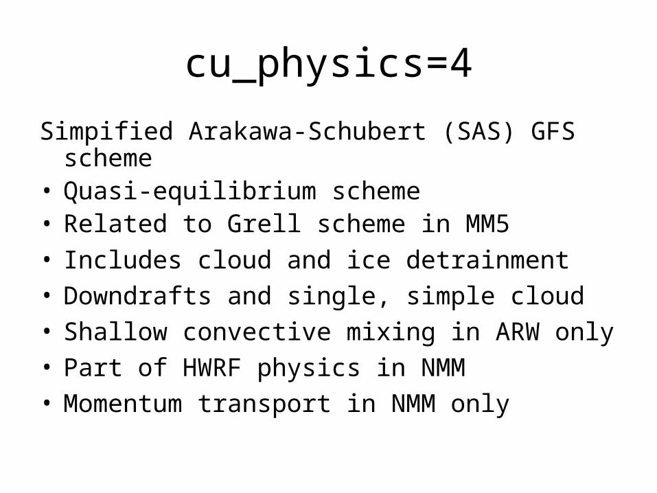
cu_physics=4

Simpified Arakawa-Schubert (SAS) GFS scheme• Quasi-equilibrium scheme• Related to Grell scheme in MM5

• Includes cloud and ice detrainment • Downdrafts and single, simple cloud • Shallow convective mixing in ARW only • Part of HWRF physics in NMM • Momentum transport in NMM only

cu_physics=5

Grell-3D• As GD, but slightly different ensemble • Includes cloud and ice detrainment • Subsidence is spread to neighboring columns

– This makes it more suitable for < 10 km grid size than other options

– cugd_avgdx=1 (default), 3 (spread subsidence) • ishallow=1 option for shallow convection • Mean feedback of ensemble is applied • Weights can be tuned (spatially, temporally) to optimize

scheme (training)

cu_physics=6

Tiedtke scheme (U. Hawaii version) (New in V3.3)

• Mass-flux scheme • CAPE-removal time scale closure • Includes cloud and ice detrainment • Includes shallow convection • Includes momentum transport

cu_physics=7

CAM Zhang-McFarlane scheme

(New in V3.3)• Mass-flux scheme • CAPE-removal time-scale closure • From current CESM climate model physics • Includes cloud and ice detrainment • Includes momentum transport

cu_physics=14

• New Simpified Arakawa-Schubert (NSAS) scheme (New in V3.3 )

• Quasi-equilibrium scheme • Updated from SAS for current NCEP GFS global

model • Includes cloud and ice detrainment • Downdrafts and single, simple cloud • New mass-flux type shallow convection

(changed from SAS) • Momentum transport

shcu_physics=2

CAM UW shallow convection (Bretherton and Park, U. Washington) • To be used with a TKE PBL scheme and a

deep scheme with no shallow convection (e.g. CESM Zhang-McFarlane)

• From current CESM climate model physics • New shallow convection driver in V3.3 • Other options such as Grell ishallow to be

moved here in the future ARW only

cudt

• Time steps between cumulus parameterization calls

• Typical value is 5 minutes

ARW only

Cumulus scheme

Recommendations about use• For dx ≥ 10 km: probably need cumulus scheme• For dx ≤ 3 km: probably do not need scheme

– However, there are cases where the earlier triggering of convection by cumulus schemes help

• For dx=3-10 km, scale separation is a question– No schemes are specifically designed with this range

of scales in mind• Issues with 2-way nesting when physics differs across

nest boundaries (seen in precip field on parent domain) – best to use same physics in both domains or 1-way

nesting

Microphysics

Atmospheric heat and moisture tendencies

Microphysical rates

Surface rainfall

Ferrier

Qi/Qs/Qg

Qv

Qc

Qr

Kessler

WSM3

Lin et al./WSM6

WSM5

Illustration of Microphysics Processes

Microphysics: Single and

Double Moment Schemes • Single-moment schemes have one prediction equation

for mass (kg/kg) per species (Qr, Qs, etc.) with particle size distribution being diagnostic

• Double-moment schemes add a prediction equation for number concentration (#/kg) per double-moment species (Nr, Ns, etc.)

• Double-moment schemes may only be double-moment for a few species

• Double-moment schemes allow for additional processes such as size-sorting during fall-out and sometimes aerosol effects on clouds

Microphysics: Fall terms

• Microphysics schemes handle fall terms for particles (usually everything except cloud water has a fall term)

• For long time-steps (such as mesoscale applications dt ~ 60 s, Vt=5 m/s), drops may fall more than a grid level in a time-step

• This requires splitting the time-step or lagrangian numerical methods to keep the scheme numerically stable

Microphysics scheme options

• Microphysics options: 13

mp_physics=1

Kessler scheme

• Warm rain – no ice

• Idealized microphysics

• Time-split rainfall

mp_physics=2

Purdue Lin et al. scheme

• 5-class microphysics including graupel

• Includes ice sedimentation and time-split fall terms

• Can be used with WRF-Chem aerosols

mp_physics=3

WSM 3-class scheme• From Hong, Dudhia and Chen (2004)• Replaces NCEP3 scheme• 3-class microphysics with ice• Ice processes below 0 deg C• Ice number is function of ice content• Ice sedimentation and time-split fall terms• Semi-lagrangian fall terms in V3.2

mp_physics=4

WSM 5-class scheme• Also from Hong, Dudhia and Chen (2004)• Replaces NCEP5 scheme• 5-class microphysics with ice• Supercooled water and snow melt• Ice sedimentation and time-split fall terms• Semi-lagrangian fall terms in V3.2

mp_physics=14

WSM 5-class scheme

• Version of WSM5 that is double-moment for warm rain processes

• 5-class microphysics with ice

• CCN, and number concentrations of cloud and rain also predicted

ARW only

mp_physics=5

Ferrier (current NAM) scheme• Designed for efficiency

– Advection of total condensate and vapour– Cloud water, rain, & ice (cloud ice, snow/graupel)

from storage arrays – assumes fractions of water & ice within the column are fixed during advection

• Supercooled liquid water & ice melt• Variable density for precipitation ice

(snow/graupel/sleet) – “rime factor”• mp_physics=85 (nearly identical) for HWRF

mp_physics=6

WSM 6-class scheme• From Hong and Lim (2003, JKMS)• 6-class microphysics with graupel• Ice number concentration as in WSM3 and

WSM5• New combined snow/graupel fall speed • Semi-lagrangian fall terms

mp_physics=16

WDM 6-class scheme • Version of WSM6 that is double-moment for

warm rain processes • 6-class microphysics with graupel • CCN, and number concentrations of cloud and

rain also predicted

ARW only

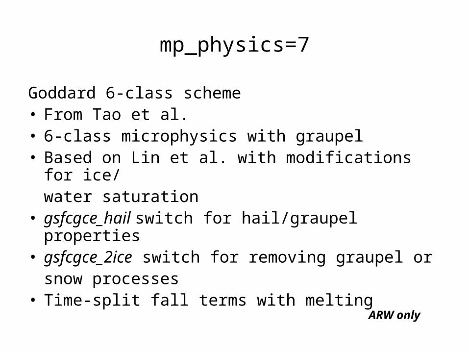
mp_physics=7

Goddard 6-class scheme • From Tao et al. • 6-class microphysics with graupel • Based on Lin et al. with modifications for ice/

water saturation • gsfcgce_hail switch for hail/graupel properties • gsfcgce_2ice switch for removing graupel or

snow processes • Time-split fall terms with melting

ARW only

mp_physics=8

Thompson et al. graupel scheme in V3.1

• Replacement of Thompson et al. (2007)

scheme that was option 8 in V3.0

• 6-class microphysics with graupel

• Ice number concentration also predicted (double-moment ice)

• Time-split fall terms

mp_physics=9

Milbrandt-Yau 2-moment scheme (New in Version 3.2)

• 7-class microphysics with separate graupel and hail

• Number concentrations predicted for all six water/ice species (double-moment) - 12 variables

• Time-split fall terms ARW only

mp_physics=10

Morrison 2-moment scheme

(since Version 3.0)

• 6-class microphysics with graupel • Number concentrations also predicted for ice,

snow, rain, and graupel (double-moment) • Time-split fall terms • Can be used with WRF-Chem aerosols (V3.3)

ARW only

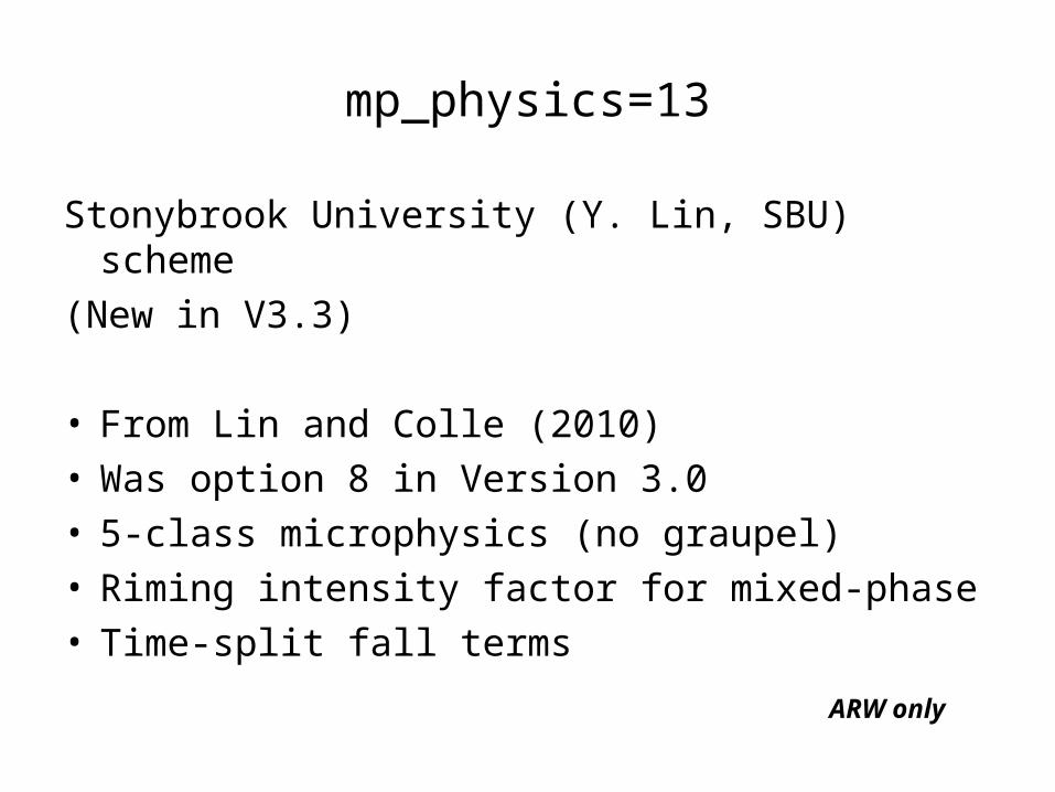
mp_physics=13

Stonybrook University (Y. Lin, SBU) scheme

(New in V3.3)

• From Lin and Colle (2010) • Was option 8 in Version 3.0 • 5-class microphysics (no graupel) • Riming intensity factor for mixed-phase • Time-split fall terms

ARW only

no_mp_heating=1

Turn off heating effect of microphysics

(Since Version 3.0)

• Zeroes out the temperature tendency • Equivalent to no latent heat • Other microphysics processes not affected

ARW only

mp_zero_out

Microphysics switch (also mp_zero_out_thresh)• 1: all values less than threshold set to zero

(except vapor)• 2: as 1 but vapor also limited ≥ 0• Note: this option will not conserve total water

• Not needed when using positive definite

advection • For NMM: recommend mp_zero_out=0

Microphysics Options

Recommendations about choice• Probably not necessary to use a graupel

scheme for dx > 10 km– Updrafts producing graupel not resolved– Cheaper scheme may give similar results

• When resolving individual updrafts, graupel scheme should be used

• All domains use same option

Rainfall Output (1)

• Cumulus and microphysics can be run at the same time

• ARW outputs rainfall accumulations since

simulation start time (0 hr) in mm • RAINC comes from cumulus scheme • RAINNC comes from microphysics scheme • Total is RAINC+RAINNC

– RAINNCV is time-step value – SNOWNC/SNOWNCV are snow sub-set of

RAINC/RAINNCV (also GRAUPELNC, etc.)

ARW only

Rainfall Output (2)

Options for “buckets” • prec_acc_dt (minutes) - accumulates separate prec_acc_c,

prec_acc_nc, snow_acc_nc in each time window (we recommend prec_acc_dt is equal to the

wrf output frequency to avoid confusion) • bucket_mm - separates RAIN(N)C into RAIN(N)C and

I_RAIN(N)C to allow accuracy with large totals such as in multi-year accumulations – Rain=I_RAIN(N)C*bucket_mm + RAIN(N)C – bucket_mm=100 mm is a reasonable bucket value – bucket_J also for CAM and RRTMG radiation budget

terms (1.e9 J/m2 recommended)

ARW only

Physics Interactions

Direct Interactions of Parametrizations

Turbulence/Diffisuion options

• Diffisuion options: 2

• Damping options: 3

Physics Summary and Plans

Acknowledgements: Thanks to presentations of NCAR/MMM Division for providing excellent starting point for this talk.

Thanks for attending….