lable at ScienceDirect

Atmospheric Environment 81 (2013) 421e432

Contents lists avai

Atmospheric Environment

journal homepage: www.elsevier .com/locate/atmosenv

WRF-Chem simulation of NOx and O3 in the L.A. basin during CalNex-2010

Dan Chen a, b, *, 1, Qinbin Li a, b, Jochen Stutz a, b, Yuhao Mao a, Li Zhang a, 2, Olga Pikelnaya a,Jui Yi Tsai a, Christine Haman c, Barry Lefer c, Bernhard Rappenglück c, Sergio L. Alvarez c,J. AndrewNeuman d, James Flynn c, JamesM.Roberts d, JohnB.Nowak e, d, Joost deGouw d, e,John Holloway e, d, Nicholas L. Wagner d, e, Patrick Veres d, e, Steven S. Brown d,Thomas B. Ryerson d, Carsten Warneke d, e, Ilana B. Pollack d, e

a Department of Atmospheric and Oceanic Sciences, University of California, Los Angeles, USAb Joint Institute for Regional Earth System Science and Engineering (JIFRESSE), UCLA, USAc Department of Earth and Atmospheric Science, University of Houston, USAd NOAA Earth System Research Laboratory (ESRL), Chemical Sciences Division, Boulder, CO, USAe Cooperative Institute for Research in Environmental Sciences (CIRES), University of Colorado Boulder, Boulder, CO, USA

h i g h l i g h t s

� NOx emissions and O3 chemistry in the Los Angeles Basin are evaluated.� NOx is overestimated in the baseline scenario (24% reduction relative to NEI’05).� A 45% reduction of NOx emissions relative to NEI’05 significantly improves the comparison of model to observations.� Modeled WeekendeWeekday differences are much smaller, indicating weekend NOx emissions are still overestimated.� Improved understanding of volatile organic compound emissions and photochemical processing on weekdays are needed.

a r t i c l e i n f o

Article history:Received 23 January 2013Received in revised form29 August 2013Accepted 31 August 2013

Keywords:CalNexWRF-Chem evaluationOzoneNOx

L.A. basin

* Corresponding author.E-mail addresses: dchen@ucar.edu, rainycd@gmail

1 Now at: National Center for Atmospheric Researc2 Now at: Department of Mechanical Engineering,

1352-2310/$ e see front matter � 2013 Elsevier Ltd.http://dx.doi.org/10.1016/j.atmosenv.2013.08.064

a b s t r a c t

NOx emissions and O3 chemistry in the Los Angeles (L.A.) Basin during the CalNex-2010 field campaign(MayeJune 2010) have been evaluated by analyzing O3 and NOy (NO, NO2, HNO3, PAN) observations usinga regional air quality model (WRF-Chem). Model simulations were conducted at 4-km spatial resolutionover the basin using the Carbon-Bond Mechanism version Z (CBM-Z) and NOx emissions reduced by 24%relative to 2005 National Emissions Inventory (NEI’05), according to recent state emission statistics(BASE_NOx scenario). In addition, a 22e26% NOx emission reduction from weekday to weekend wasapplied. WRF-Chem reproduced the observed diurnal cycle and day-to-day variations in surface O3, Ox,HNO3 and HCHO (correlation r2 ¼ 0.57 � 0.63; pairs of data n > 400; confidence value p < 0.01) at theCalNex supersite at Caltech but consistently overestimated surface NO and NO2. A 45% reduction of NOx

emissions relative to NEI’05 (LOW_NOx scenario), as suggested by the OMI-NO2 column trend in Cali-fornia over the same period, improved the agreement of modeled NO2, NOx, and O3 with observations onweekdays. Three-dimensional distributions of daytime O3 and NOy were compared with five daytimeNOAA WP-3D flights (three on weekdays and two on weekends) to study the Weekend-to-Weekday(WE-to-WD) effects by using the LOW_NOx scenario. Aircraft data showed a 17.3 ppb O3 increase anda 54% NOy reduction in the boundary layer on weekends relative to weekdays, while modeled WE-to-WDdifferences were much smaller, with a 2.9 ppb O3 increase and 16% NOy reduction only. Model results onweekends underestimated O3 by 23% and overestimated NOy and HNO3 by 40% and 27%, respectively,which may indicate that weekend NOx emissions (45% reduction relative to NEI’05 with a 22e26%reduction on weekends compared to weekdays) were still overestimated in the model. Comparisons ofPAN to HNO3 ratios also indicated that the enhanced photochemistry on weekends was not well

.com (D. Chen).h, Boulder, Colorado, USA.University of Colorado Boulder, Boulder, Colorado, USA.

All rights reserved.

D. Chen et al. / Atmospheric Environment 81 (2013) 421e432422

represented in the model. Although modeled weekday O3 was close to the observations in the boundarylayer, modeled PAN and HNO3 were overestimated by 30% and 22%, respectively, and modeled NOy wasunderestimated by 24% on weekdays. Interpreted as emission ratios, the slopes of volatile organiccompound (VOC) species versus CO concentrations indicated that speciated VOC emissions in the modelwere not accurately represented, impacting the photochemistry in the model. These findings argue forthe need to improve our understanding of VOC emissions and their photochemical processing in themodel.

� 2013 Elsevier Ltd. All rights reserved.

1. Introduction

The Los Angeles (L.A.) basin has been ranked as the mostpollutedmegacity in the U.S. with respect to O3 (The American LungAssociation, 2012). High O3 in the L.A. basin results from theextremely high emission of O3 precursors, nitrogen oxidesNOx ¼ NO þ NO2 and volatile organic compounds (VOC). Over thepast two decades (1985e2005), the total emissions of VOC and NOx

in the South Coast Air Basin (SCAB) have been reduced significantly(California Air Resources Board, CARB, 2012c; data available athttp://www.arb.ca.gov/app/emsinv/emssumcat.php). Althoughdecades of emission reductions have been effective at mitigating O3levels, many monitoring locations in the SCAB are still not inattainment of the National Ambient Air Quality Standard (NAAQS)(www.aqmd.gov).

Regional air quality models are useful tools to study this airpollution problem. Previous modeling studies have revealed thatthe photochemical pollution in the basin is exacerbated by the factthat the high emission intensity area is surrounded by mountains,which tends to trap the air pollution as it is blown eastward by theprevailing westerly winds (e.g. Lu and Turco, 1995, 1996). However,the application of regional models to the L.A. basin is challengingdue to the combined effects of complex terrain-meteorology andhigh emissions in the basin. The challenges and the evaluations ofthe terrain-meteorology simulations using the WRF-Chem modelfor the L.A. basin have been described in an accompanying paper,Chen et al. (2013). The primary goal of the current paper is toevaluate the model capability to simulate the photochemistry inthe basin.

Another motivation for revisiting O3 pollution in the basin is theneed to understand the effect of NOx emissions, which changes interms of the total amounts, major sources and temporal variation.Many studies have observed the recent decrease of NOx emissionsin the U.S. andmost of them show evidence that the decrease is dueto the implementation of NOx control technology in power plants(e.g. Kim et al., 2006, 2009). Fuel-consumption-based calculationsand ambient measurements have also been used to estimateexhaust NOx emissions from mobile sources (e.g. Parrish, 2006;Harley et al. 2005). A 9e10% per year reduction trend was foundduring the 2007e2009 period (McDonald et al., 2012) in the L.A.basin, where mobile sources account for w80% of total NOx emis-sions. In the study of Russell et al. (2010), OMI satellite data andground surface observational data were used to constrain NOx

emissions in the California region. The observed decrease of NO2vertical columns in Los Angeles and the surrounding cities was 9%per year for 2005e2008. Brioude et al. (2011) presented top-downestimates of anthropogenic NOx surface fluxes and found that NOx

emissions were 32 � 10% lower in the L.A. county relative to NEI’05for 2010. However, statistics from the California Air ResourcesBoard (CARB) show a much slower reduction. CARB reports adecrease in total NOx from 2005 to 2010 of around 24% (CARB,2012c; data available at http://www.arb.ca.gov/app/emsinv/emssumcat.php). In addition to the uncertainties of total NOx

emission reductions, observations also showed a large Weekend-

to-Weekday (WE-to-WD) NOx emission reduction, which leads tohigher O3 on weekends (Pollack et al., 2012; Russell et al., 2010).

In this work, we apply theWRF-Chemmodel to simulate O3 andNOy species for selected days in MayeJune 2010 in the L.A. Basinduring the CalNex-2010 intensive field experiment, focusing onthreeweekday daytime flights of the NOAAWP-3D research aircrafton May 4, 14 and 19, and two weekend daytime flights on May 16and June 20. We conducted simulations at 4-km spatial resolutionover the L.A. Basin using the Carbon-Bond Mechanism version Z(CBM-Z). In an accompanying paper (Chen et al., 2013), wedescribed the model configurations and evaluations of meteoro-logical and carbon monoxide (CO) predictions. This study evaluateschemical predictions resulting from two adjusted NOx emissionscenarios. The monitoring database includes CARB stations, surfaceobservations on the campus of the California Institute for Tech-nology (Caltech), and the aircraft data. Chemical species evaluatedin our study include ozone (O3), NOx (¼ NO þ NO2), formaldehyde(HCHO), nitric acid (HNO3) and peroxyacetyl nitrate (PAN).

In this manuscript, we validate the model chemical predictionsthrough comparisons of the modeled surface O3, NOy, NO, NO2, Ox,HCHO and HNO3 mixing ratios with those measured at the Caltechsite. The NOx emission inventory is evaluated by comparing thesimulated O3 and NOx to measurements at 20 CARB surface sites.More definitive conclusions regarding the total NOx emissions,model capabilities and Weekend-to-Weekday (WE-to-WD) effectsare obtained by comparing the model against daytime aircraft ob-servations on weekdays and weekends. The WRF-Chem modeldeficiencies are discussed in the context of these comparisons.

2. Methodology

2.1. WRF-Chem description

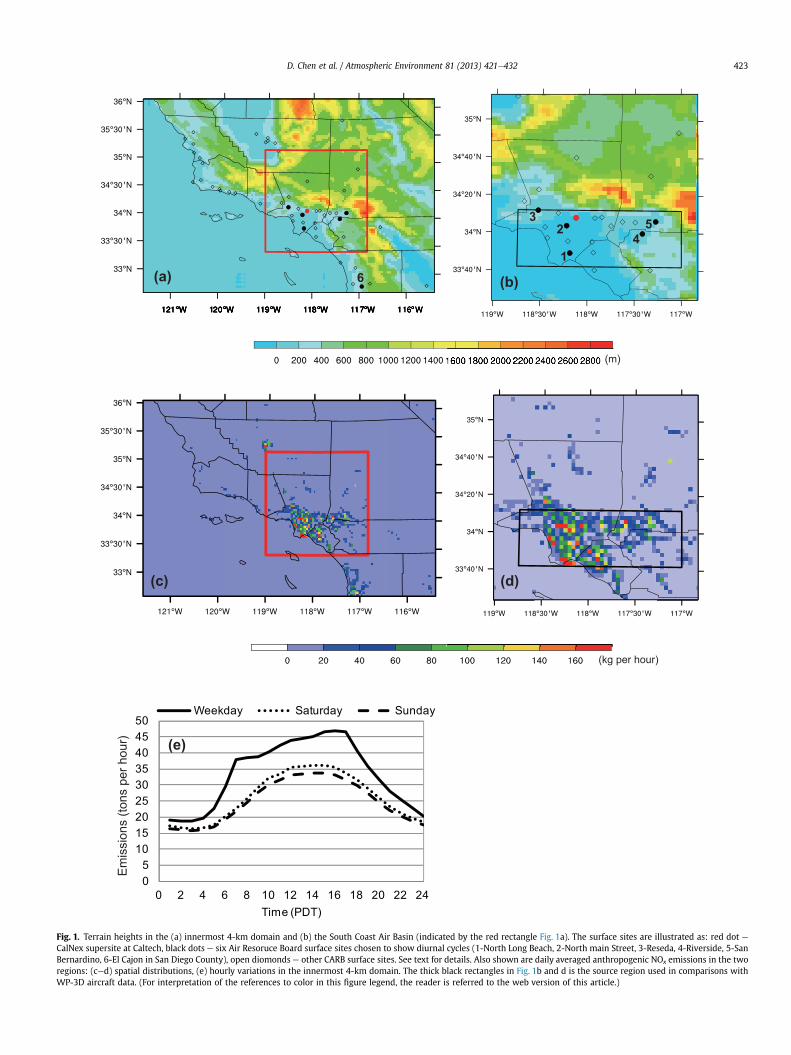
The Weather Research and Forecasting (WRF) model coupledwith online chemistry (WRF-Chem) version 3.1.1 was used in thisstudy (http://ruc.noaa.gov/wrf/WG11/; Grell et al., 2005; Fast et al.,2006). Three nested domains with 36-, 12- and 4- km horizontalresolution cover the regions of the western United States, Californiaand the L.A. basin, respectively (Fig. 1 in Chen et al., 2013). Thetopography in the 4-km domain is shown in Fig. 1a. There are 30vertical layers extending from the surface to 100 hPa, with a finerresolution near the surface.

Initial and lateral boundary conditions (LBC) for meteorologicalvariables were obtained from the North American Regional Rean-alysis (NARR) 32 km 3-hourly data (Mesinger et al., 2006). Lateralboundary conditions of trace gases in the model were taken fromthe averages of mid-latitude aircraft profiles. The simulation periodextended from May 15 to June 15, 2010. The model simulationswere re-initialized at 00:00 UTC every 72 h to mitigate the prob-lems of systematic error growth in long integrations (Lo et al.,2008). The Carbon-Bond Mechanism version Z (CBM-Z) was usedfor the chemical simulations. Further details of the model config-uration can be found in an accompanying paper by Chen et al.(2013).

(m)

(a)(b)

(m)(m)

05

101520253035404550

0 2 4 6 8 10 12 14 16 18 20 22 24Time (PDT)

Weekday Saturday Sunday

(d)(c)

(e)

1

2

3

4

5

6

(kg per hour)

Emis

sion

s (to

ns p

er h

our)

Fig. 1. Terrain heights in the (a) innermost 4-km domain and (b) the South Coast Air Basin (indicated by the red rectangle Fig. 1a). The surface sites are illustrated as: red dot eCalNex supersite at Caltech, black dots e six Air Resoruce Board surface sites chosen to show diurnal cycles (1-North Long Beach, 2-North main Street, 3-Reseda, 4-Riverside, 5-SanBernardino, 6-El Cajon in San Diego County), open diomonds e other CARB surface sites. See text for details. Also shown are daily averaged anthropogenic NOx emissions in the tworegions: (ced) spatial distributions, (e) hourly variations in the innermost 4-km domain. The thick black rectangles in Fig. 1b and d is the source region used in comparisons withWP-3D aircraft data. (For interpretation of the references to color in this figure legend, the reader is referred to the web version of this article.)

D. Chen et al. / Atmospheric Environment 81 (2013) 421e432 423

D. Chen et al. / Atmospheric Environment 81 (2013) 421e432424

The reference anthropogenic emission inventory used in thisstudy was based on the National Emission Inventory 2005 (NEI’05,U.S. EPA, 2010; hereafter referred as NEI’05_REF). The gridded (4-km resolution) and point source hourly emissions files originatedfrom ftp://aftp.fsl.noaa.gov/divisions/taq/emissions_data_2005/.Weekday and weekend emissions were both considered. Specificdetails of the inventory, including the activity data, mobile on-roadand mobile non-road emissions and uncertainties have beendescribed by Kim et al. (2011). The biogenic emissions werecalculated from the Guenther online scheme in the model(Guenther et al., 1993, 1994)

Fig. 1c and d show the spatial distribution of daily averagedanthropogenic NOx emissions over the innermost domain and theSouth Coast Air Basin (SCAB) area. At 4-km resolution, the in-ventory explicitly resolves contributions from several urban centerswith high emission intensities (“hot spots” in Fig.1d): a) cities withhigher levels of urbanization and motorization in the SCAB, such asLong Beach (118.2�W, 33.8�N), Los Angeles (118.4�W, 33.9�N),Irvine (117.8�W, 33.7�N) where the transportation sector contrib-utes 70e85% to the total NOx emissions and up to 50% to the VOCemissions, b) densely populated cities such as Riverside (117.3�W,33.9�N) and San Bernardino (117.3�W, 34.1�N), with multiplesources including heavy industrial manufacturing. The analysis inthis study is mainly focused on the source region, which is definedby the black rectangle in Fig. 1b and d.

Weekend-to-Weekday (WE-to-WD) emission changes are alsoconsidered in the NEI’05_REF. Compared to NOx emissions onweekdays, the emissions on Saturday and Sunday are 22% and 26%lower respectively, due to reduced diesel truck traffic duringweekends (e.g. Dreher et al., 1998; Chinkin et al., 2003; Pollacket al., 2012). In addition, the hourly NOx variations on weekendsalso showa comparatively smaller increase during themorning andafternoon rush hours (Fig. 1e) compared to weekdays. Unlike NOx

emissions, which are dominated by on-road vehicles, VOC emis-sions also had significant contributions from area sources (solvent,paint and other residential sources) in the basin (CARB, 2012c; dataavailable at http://www.arb.ca.gov/app/emsinv/emssumcat.php).In the model, VOC species are lumped into several functionalgroups based on structure and reactivity (Carter, 1994). Weekendemission changes of VOC vary by groups, with the ratios rangingfrom 0.89 to 1.14. The reactivity of the VOC groups is calculatedbased on the reactivity scales of the main compounds (Carter, 2013;data available at http://www.engr.ucr.edu/wcarter/SAPRC/). Theestimated total VOC reactivity R during the weekends is close tothat on weekdays with a 1.02e1.04 weekend/weekday ratio.Overall, the inventories indicate that the NOx/R ratio decreases onweekends in the basin.

The reference emission inventory NEI’05 was developed by EPAbased on a reduced level of effort. Part of this reduced effortinvolved using some NEI 2002 data in the NEI 2005 as surrogatesfor emission data representing 2005, including some emissionsfrom point and nonpoint sources. The on-road mobile sourcesemission estimates were based on 2005 vehicle miles traveled

Table 1Some chemical composition measurements aboard the NOAA WP-3D aircraft during Cal

Chemical species Measurement technique Re

O3, NO, NO2 Chemiluminescence detector (RPo

CO VUV CO Instrument (HHNO3 Chemical Ionization Mass Spectrometry (NHCHO PTR-MS about every 17 s (d

20PAN Chemical Ionization Mass Spectrometry (ZNO, NO2, O3, NO3, N2O5 Cavity Ringdown (D

(VMT) and a 2005 run of the National Mobile Inventory Model(NMIM) representing 2005 level. The use of 2002 data as a surro-gate for the point and nonpoint sources in NEI’05 increased theemission inventory uncertainties in our study. To reflect theemission changes from 2005 to 2010, two emission scenarios weregenerated based on NEI’05_REF by applying scaling factors. In thebaseline case (BASE_NOx), anthropogenic NOx was reduced by 24%according to CARB emission projections (CARB, 2012c; data avail-able at http://www.arb.ca.gov/app/emsinv/emssumcat.php) for theSouth Coast Air Basin. These ratios were applied evenly toweekday,Saturday, and Sunday emission data for each grid box based onNEI’05_REF. In the low NOx case (LOW_NOx), we decreased the NOx

emission by 45% relative to NEI’05_REF, based on the 9% per yearreduction reported by Russell et al. (2010).

2.2. Observations

Surface observations at the Caltech supersite (www.esrl.noaa.gov/csd/projects/calnex/; 34.138 �N, 118.126 �W, 246 m above sealevel -asl) and California Air Resource Board (CARB) sites (Fig. 1b)were used in this study. A detailed description of the Caltech supersite is included in Chen et al. (2013). Observational data at the Cal-tech super site (red dot on Fig. 1b) include 1-min averaged data forO3, NO, andNO2 (for instrument details refer to Lefer et al., 2010), NI-PT-CIMS Instrumentmeasured 1-min HNO3 (Veres et al., 2008), and1-min HCHO using the fluorometric Hantzsch reaction(Rappenglück et al., 2010;Warnekeet al., 2011; 10%uncertainty).Weaveraged the aforementioned data to an hourly temporal resolutionfor comparison with the model hourly outputs. It should be notedthat HCHOwas alsomeasured by theDifferential Optical AbsorptionSpectroscopy (DOAS), which retrieved the average concentrationsalong the light path (a few kilometers). The two HCHOmethods didnot agree quantitatively, which may add some uncertainty to theHCHO comparison (see Warneke et al., 2011 for details).

In addition to the Caltech super site, CARB also measured hourlyO3, NO, NO2 and NOx throughout the L.A. basin. The concentrationsof NO and NOx were measured independently by chem-iluminescence detectors and the concentrations of NO2 werecalculated by subtracting the measured NO from measured NOx

(CARB 2007; report available at http://www.arb.ca.gov/aaqm/qa/qa-manual/vol4/measurement_of_nox.pdf). We chose six of theCARB sites (black dots on Fig. 1b) to show their diurnal cycles in ouranalysis. Three of the sites were in the source region: one coastalsite in Long Beach (33.82 �N, 118.18 �W), near downtown LA onNorth Main Street (34.07 �N, 118.23 �W), and the third in Reseda(34.20 �N, 118.53 �W). Two other sites were in Riverside (34.00 �N,117.41 �W) and in San Bernardino (34.11 �N,117.27 �W) e these twosites are downwind of the concentrated urban source region andgenerally experience the highest 8-h O3 in the basin. The site in SanDiego County (32.79 �N, 116.94 �W) was chosen as a relativelyunpolluted location. Other CARB sites (open diamonds on Fig.1b) inthe SCAB, of which 20 were located in the source region (smallblack rectangles in Fig. 1b and d), were also used for comparisons.

Nex period.

ference Uncertainties

yerson et al., 1999, 2000, 2001, 2003,llack et al., 2010)

1 sigma uncertainty

olloway et al. 2000) 5%euman et al., 2002, 2003) �(15% þ 100ppt)e Gouw et al., 2003; Warneke et al.,03, 2011)

Between 30% at low altitude and100% at high altitude

heng et al., 2011) 20% þ 5 pptvube et al., 2006) 20%

Table 2WRF-Chem simulated (BASE) and observed (OBS) surface chemical species concentrations (O3, NOy, NO, NO2, HCHO, HNO3) at the Caltech super site for May 27-June 15, 2010.Also listed are model biases, standard deviations (S.D.), root mean square error (RMSE) and correlations (r2) between model results and observations. Model results aresimulated by using emission scenario BASE_NOx. Units:ppb (pairs of data n > 400).

Mean S.D Bias BASE-OBS RMSE r2 Daytime meana Nighttime meanb

OBS BASE OBS BASE OBS BASE OBS BASE

O3 36.2 25.6 19.5 18.3 �10.6 12.2 0.63 56.8 47.4 21.6 9.9NOx 21.8 27.7 10.0 13.0 6.1 15.6 0.01 21.6 20.8 19.9 30.8NO 2.4 5.9 4.5 7.3 3.6 7.5 0.07 2.2 5.5 0.8 2.1NO2 13.0 22.3 7.0 10.0 9.3 10.7 0.06 10.6 15.4 15.1 28.9Ox 49.4 47.7 16.8 13.8 �1.7 8.8 0.73 67.5 62.4 36.9 38.6HCHO 1.5 2.4 0.8 0.9 0.9 0.6 0.57 2.1 2.8 1.0 2.0HNO3 3.1 3.0 3.1 2.8 �0.2 1.9 0.63 4.6 5.6 1.8 1.3

a Daytime: 12:00e18:00 PDT.b Nighttime: 22:00e3:00 PDT.

D. Chen et al. / Atmospheric Environment 81 (2013) 421e432 425

The NOAAWP-3D, based out of Ontario, CA, made in situ verticalprofile measurements of a suite of chemical species (http://www.esrl.noaa.gov/csd/projects/calnex/). In this work, we focused onfive flights including three weekday daytime flights on May 4, 14,and 19, and two weekend daytime flights on May 20 and June 20.The selected days were dominated by westerly flow during thedaytime and stagnant conditions during the nighttime. The WRF-Chem model performed well in terms of meteorological pre-dictions during these days (Chen et al., 2013). The flight tracks in theSCAB area (Fig. 1b) are shown in Fig. 3 of Chen et al. (2013). For thepurpose of determining NOx emissions over the L.A. source region,only measurements over land and within the source region (shownby a small black rectangle in Fig. 1b and d) were analyzed. Mea-surements over the Pacific Oceanwere excluded. A partial list of thechemical species measured onboard the aircraft is shown in Table 1.

3. Results and discussions

3.1. Comparisons at surface sites

We evaluated WRF-Chem simulations against surface observa-tions at the Caltech super site and CARB sites. The measurements at

Table 3Same as Table 2, but for surface O3, NOx ¼ NO þ NO2 and Ox ¼ O3þNO2 at CARB sites forBASE_NOx emission scenarios respectively. Units:ppb (pairs of data n > 500).

Mean Bias

OBS LOW BASE LOW e

O3 At single siteNorth Long Beach 31.9 20.3 17.3 �11.6North Main Street 28.9 22.5 17.1 �6.4Reseda 41.0 34.4 31.7 �6.7Riverside 43.8 38.2 32.8 �5.7San Bernadino 36.4 36.8 29.7 0.4El Cajon 33.7 34.4 32.6 0.720 sites AverageNighttime 23.8 13.9 9.4 �9.9Weekday daytime 48.7 49.8 43.0 1.1Weekend daytime 62.7 54.5 51.6 �8.1

NOx At single siteNorth Long Beach 18.9 25.9 37.2 7.0North Main Street 30.9 30.1 45.2 �0.720 sites averageNighttime 14.0 20.3 29.9 6.3Weekday daytime 14.1 12.5 15.5 �1.5Weekend daytime 9.1 9.0 11.3 �0.1

Ox At single siteNorth Long Beach 42.1 36.1 36.8 �6.0North Main Street 46.9 42.7 42.4 �4.3Reseda 51.5 41.4 41.7 �10.1Riverside 53.6 49.2 48.2 �4.4San Bernadino 53.4 49.6 48.0 �3.8El Cajon 41.5 42.8 43.0 1.3

the Caltech super site were compared to simulations with thebaseline emission scenario (BASE_NOx). CARB observations werecompared with model results using two emission scenariosBASE_NOx and LOW_NOx. Modeled and observed hourly concen-trations, model bias, standard deviations (S.D.), root mean squareerror (RMSE) and correlations r2 are listed in Tables 2 and 3. Tovalidate the model performance during the day and night, modeledand observed concentrations for afternoon hours (12:00e18:00PDT) and nighttime hours (22:00e3:00 PDT) are also listed.

Fig. 2 shows the hourly surface O3, NOx, NO, NO2, Ox, HCHO andHNO3 at the Caltech super site for May 27-June 15. Modeled NOx

was calculated as the sum of NO and NO2. Compared to observa-tions, the high O3 levels during May 29e30 were under-predictedby 20e40 ppb by the model, in large part due to deeper thanobserved PBL heights in the model (Fig. 4, Chen et al., 2013) com-bined with the failure of meteorological and O3 simulations ofcorrectly describing the stratospheric intrusion event on May 29th(Langford et al., 2012). After excluding May 29e30, the day-to-dayvariation and diurnal cycle of O3 was well simulated (for May 27eJune 15, correlations r2 ¼ 0.63, pairs of data n > 470, confidence valuep < 0.01). The model slightly underestimated afternoon O3 by9.3 ppb (16%) but severely underestimated nighttime O3 by 11.7 ppb

May 15eJune 8, 2010. Model results are from two simulations with LOW_NOx and

RMSE r2

OBS BASE e OBS LOW BASE LOW BASE

�14.6 12.2 12.2 0.12 0.12�11.8 11.6 11.0 0.57 0.56�9.3 11.4 12.0 0.61 0.57

�11.1 12.5 12.0 0.70 0.71�6.7 13.3 12.6 0.71 0.74�1.1 10.9 10.5 0.42 0.46

�14.3 16.3 18.7 0.10 0.13�5.7 12.4 11.9 0.48 0.51

�11.1 13.2 15.4 0.70 0.64

18.3 21.8 30.2 0.10 0.1014.4 17.6 21.9 0.20 0.19

13.7 13.7 20.5 0.14 0.161.5 9.0 9.6 0.22 0.292.1 7.3 9.8 0.35 0.38

�5.3 7.1 7.4 0.40 0.36�4.5 8.4 8.5 0.61 0.55�9.8 10.1 10.6 0.61 0.57�5.4 12.3 12.5 0.64 0.62�5.4 11.8 12.3 0.69 0.651.5 10.1 10.1 0.45 0.44

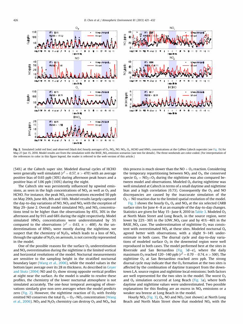
Fig. 2. Simulated (solid red line) and observed (black dot) hourly averages of O3, NOy, NO, NO2, Ox, HCHO and HNO3 concentrations at the CalNex Caltech supersite (see Fig. 1b) forMay 27-Jun 15, 2010. Model results are from the simulation with the BASE_NOx emission scenarios (see text for details). The three weekends are color-coded. (For interpretation ofthe references to color in this figure legend, the reader is referred to the web version of this article.)

D. Chen et al. / Atmospheric Environment 81 (2013) 421e432426

(54%) at the Caltech super site. Modeled diurnal cycles of HCHOwere generally well simulated (r2 ¼ 0.57, n > 470) with an averagepositive bias of 0.65 ppb (30%) during afternoon peak hours and apositive bias of 1.06 ppb (110%) during the night.

The Caltech site was persistently influenced by upwind emis-sions, as seen in the high concentrations of NOx as well as O3 andHCHO. For instance, the peak NOx concentrations exceeded 50 ppbonMay 29th, June 4th, 8th and 14th. Model results largely capturedthe day-to-day variations of NO, NO2 and NOx with the exception ofMay 29eJune 2. Overall model simulated NO2 and NOx concentra-tions tend to be higher than the observations by 45%, 30% in theafternoon and by 91% and 68% during the night respectively. Modelsimulated HNO3 concentrations were underestimated by 5%compared to the observations (r2 ¼ 0.63, n > 400). As the un-derestimations of HNO3 were mostly during the nighttime, wesuspect that the chemistry of N2O5, which leads to a loss of NOxthrough the uptake of N2O5 on aerosols, is not correctly representedin the model.

One of the possible reasons for the surface O3 underestimationand NOx overestimation during the nighttime is the limited verticaland horizontal resolutions of the model. Nocturnal measurementsare sensitive to the sampling height in the stratified nocturnalboundary layer (Wang et al., 2006), while the model values in thebottom layer average over its 28 m thickness. As described in Geyerand Stutz (2004) NO and O3 show strong opposite vertical profilesat night near the surface. As the model is unable to resolve theseprofiles, the chemistry of the lower nocturnal atmosphere is notsimulated accurately. The one-hour temporal averaging of obser-vations similarly give non-zero averages when the model predictszero (Fig. 2). However, the nighttime reaction of O3 with freshlyemitted NO conserves the total Ox ¼ O3þNO2 concentration (Wanget al., 2006). NO3 and N2O5 chemistry can destroy O3 and NOx, but

this process is much slower than the NOþ O3 reaction. Consideringthe temporary repartitioning between NO2 and O3, the conservedspecie Ox ¼ NO2þO3 during the nighttime was also compared be-tween model and observations. Modeled Ox during nighttime waswell simulated at Caltech in terms of a small daytime and nighttimebias and a high correlation (0.73). Consequently the O3 and NOdiscrepancies are caused by the inaccurate simulation of theO3 þ NO reaction due to the limited spatial resolution of the model.

Fig. 3 shows the hourly O3, Ox and NOx at the six selected CARBsurface sites for June 4e8 as an example of the day-to-day changes.Statistics are given for May 15eJune 8, 2010 in Table 3. Modeled O3at North Main Street and Long Beach, in the source region, werelower by 22%e36% in the LOW_NOx case and by 41%e46% in theBASE_NOx case. The underestimation of nighttime O3 was consis-tent with overestimated NOx at these sites. Modeled nocturnal Ox

agreed better with observations, with a slight 9e14% under-estimate in both cases. The diurnal cycle and day-to-day varia-tions of modeled surface O3 in the downwind region were wellreproduced in both cases. The model performed best at the sites inRiverside and San Bernardino (Fig. 3dee), where the dailymaximum O3 reached 120e140 ppb (r2 ¼ 0.70 � 0.74, n > 500). Thenighttime O3 at San Bernardino reached zero ppb. The strongdiurnal cycle may indicate that the O3 formation at the two sites isaffected by the combination of daytime transport from the down-town L.A. source region and nighttime local emissions; both factorsare well represented for the two sites in the model. The worst O3and Ox simulation occurred at Long Beach (Fig. 3a), where bothdaytime and nighttime values were underestimated. Two possibleexplanations for this finding are an excess in NOx emissions or aweaker sea breeze at Long Beach in the model.

Hourly NOx (Fig. 3), Ox, NO and NO2 (not shown) at North LongBeach and North Main Street show that modeled NOx with the

North Long Beach

0

50

100

150

O3 (p

pb

)

CARBLOW_NOxBASE_NOx

Riverside-Rubidoux

0

50

San Bernardino El Cajon

020

40

60

80

100

NO

x (p

pb

)

0

20

40

4 5 6 7 8Jun

4 5 6 7 8Jun

4 5 6 7 8Jun

4 5 6 7 8 9Jun

North Main StreetCARB

4 5 6 7 8Jun

LOW_NOxBASE_NOx

Reseda

100

150

4 5 6 7 8 9Jun

CARBLOW_NOxBASE_NOx

CARBLOW_NOxBASE_NOx

CARBLOW_NOxBASE_NOx

CARBLOW_NOxBASE_NOx

0

50

100

150

Ox (p

pb

)

Fig. 3. Simulated (solid lines) and observed (black dot) hourly averages of O3, NOx and Ox concentrations at six CARB sites: a) North Long Beach, b) North Main Street, c) Reseda, d)Riverside, e) San Bernardino and f) El Cajon (see Fig. 1b for locations) for June 4e8, 2010. Model results from two simulations are shown: red lines eLOW_NOx; blue lines e

BASE_NOx. Units:ppb. (For interpretation of the references to color in this figure legend, the reader is referred to the web version of this article.)

D. Chen et al. / Atmospheric Environment 81 (2013) 421e432 427

LOW_NOx emission scenario (red solid line) agreed better with theobservations (Table 3). Correspondingly, model simulated O3 in thesource region was also improved with a relatively small bias(Table 3). However, nighttime O3 and daytime Ox at Long Beach andNorth Main Street, in the source region, was still severely under-estimated, and modeled NOx at Long Beach was still 37% higher inthe LOW_NOx case.

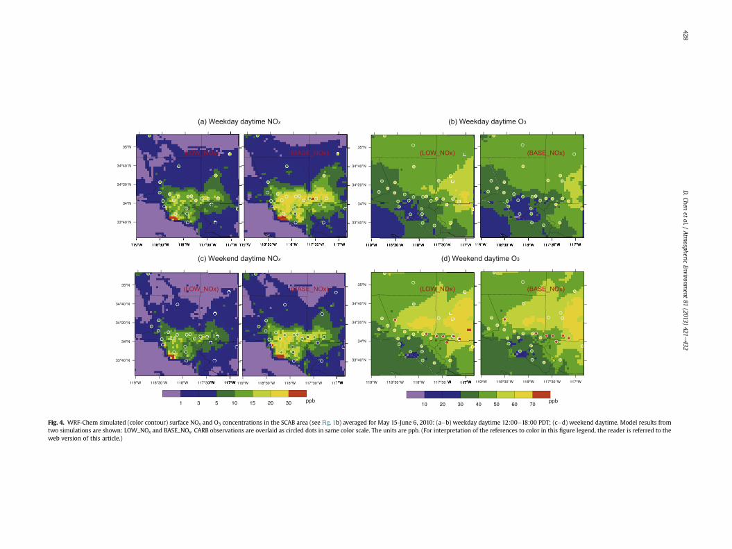
The spatial distributions of model averaged NOx and O3 duringdaytime on weekdays and weekends in the SCAB area (Fig. 1b andd) for May 15-June 8, 2010 are plotted in Fig. 4, to better illustratethe modeled NOxeO3 response to different NOx emissions in thebasin. Daytime values were averaged from 12:00e18:00 PDT for 17weekdays (top panels) and 8 weekend days (bottom panels). O3data on May 29e30 (weekends) were excluded due to knownproblems in the model (details in Section 3.2, Chen et al., 2013).Model simulations were performed with two emission scenariosLOW_NOx and BASE_NOx. The CARB observations (circled dots) areoverlaid for comparisons. Table 3 lists the quantitative model per-formance statistics for NOx and O3 using observations at 20 CARBsites in the source region.

Modeled daytime O3 increased as NOx emission decreased in thebasin, showing that the SCAB is NOx-saturated (e.g. Qin et al., 2004).However, modeled weekend O3 was not as sensitive to NOx emis-sions compared to weekday O3: during weekdays, O3 increased by6.8 ppb in the model with NOx emission changing from BASE_NOx

to LOW_NOx (Table 3), while the modeled O3 increase was only2.9 ppb during weekends. As there is a 22e26% NOx emission

reduction fromweekdays to weekends in the model, it is likely thatmodeled weekend O3 production is less NOx-saturated and that thesystem is shifted towards the crossover point between the NOx-limited and NOx-saturated regimes compared to the case onweekdays. Compared to observations, modeled daytime O3 biaseswere slightly smaller in the LOW_NOx case, both on weekdays andweekends, but still reached �8.1 ppb on weekends (Table 3).

3.2. Weekday-weekend effects

Both model and observations showed Weekend-to-Weekday(WE-to-WD) effects with decreased NOx concentrations andincreased O3 levels during the weekend (Fig. 4). The weekend O3effect in the South Coast Air Basin (SCAB), where daytime surfaceozone concentrations tend to be higher on weekends than onweekdays, has been studied extensively [e.g. Blanchard andTanenbaum, 2003; Chinkin et al., 2003; Fujita et al., 2003; Marrand Harley, 2002b; Qin et al., 2004; Yarwood et al., 2003; Pollacket al., 2012]. Decreased NOx emissions on weekends, with a corre-sponding acceleration of radical chemistry is considered to be themajor cause of increased weekend ozone concentrations [e.g.Blanchard and Tanenbaum, 2003; Fujita et al., 2003; Marr andHarley, 2002a, 2002b; Murphy et al., 2007; Tonse et al., 2008;Yarwood et al., 2003, 2008; Pollack et al., 2012; Warneke et al.,2012].

In addition to surface observations, we selected five flights tolook into O3 and NOx differences three-dimensionally. Model

(a) Weekday daytime NOx

(c) Weekend daytime NOx

(b) Weekday daytime O3

(d) Weekend daytime O3

(LOW_NOx) (BASE_NOx)

(LOW_NOx) (BASE_NOx)

(LOW_NOx) (BASE_NOx)

(LOW_NOx) (BASE_NOx)

Fig. 4. WRF-Chem simulated (color contour) surface NOx and O3 concentrations in the SCAB area (see Fig. 1b) averaged for May 15-June 6, 2010: (aeb) weekday daytime 12:00e18:00 PDT; (ced) weekend daytime. Model results fromtwo simulations are shown: LOW_NOx and BASE_NOx. CARB observations are overlaid as circled dots in same color scale. The units are ppb. (For interpretation of the references to color in this figure legend, the reader is referred to theweb version of this article.)

D.Chen

etal./

Atm

osphericEnvironm

ent81

(2013)421

e432

428

WP-3D

Model

WP-3D

Model

WP-3D

Model

WP-3D

Model

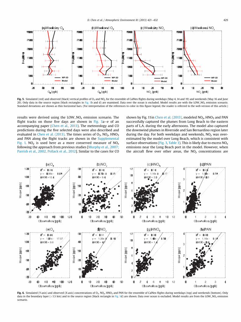
Fig. 5. Simulated (red) and observed (black) vertical profiles of O3 and NOy for the ensemble of CalNex flights during weekdays (May 4, 14 and 19) and weekends (May 16 and June20). Only data in the source region (black rectangles in Fig. 1b and d) are examined. Data over the ocean is excluded. Model results are with the LOW_NOx emission scenario.Standard deviations are shown as thin horizontal bars. (For interpretation of the references to color in this figure legend, the reader is referred to the web version of this article.)

D. Chen et al. / Atmospheric Environment 81 (2013) 421e432 429

results were derived using the LOW_NOx emission scenario. Theflight tracks on those five days are shown in Fig. 3aee of anaccompanying paper (Chen et al., 2013). The meteorology and COpredictions during the five selected days were also described andevaluated in Chen et al. (2013). The times series of O3, NOy, HNO3and PAN along the flight tracks are shown in the SupplementalFig. 1. NOy is used here as a more conserved measure of NOx

following the approach from previous studies [Murphy et al., 2007;Parrish et al., 2002, Pollack et al., 2012]. Similar to the cases for CO

Fig. 6. Simulated (Y-axis) and observed (X-axis) concentrations of O3, NOy, HNO3 and PAN fodata in the boundary layer (<1.5 km) and in the source region (black rectangle in Fig. 1d) ascenario.

shown by Fig. 11in Chen et al. (2013), modeled NOy, HNO3 and PANsuccessfully captured the plumes from Long Beach to the easternparts of L.A. during the early afternoons. The model also capturedthe downwind plumes in Riverside and San Bernardino region laterduring the day. For both weekdays and weekends, NOy was over-estimated by the model over Long Beach, which is consistent withsurface observations (Fig. 3, Table 3). This is likely due to excess NOx

emissions near the Long Beach port in the model. However, whenthe aircraft flew over other areas, the NOy concentrations are

r the ensemble of CalNex flights during weekdays (top) and weekends (bottom). Onlyre shown. Data over ocean is excluded. Model results are from the LOW_NOx emission

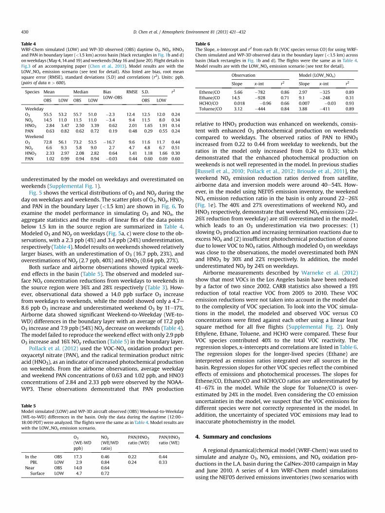
Table 6The Slope, x-Intercept and r2 from each fit (VOC species versus CO) for using WRF-Chem simulated and WP-3D observed data in the boundary layer (<1.5 km) acrossbasin (black rectangles in Fig. 1b and d). The flights were the same as in Table 4.Model results are with the LOW_NOx emission scenario (see text for detail).

Observation Model (LOW_NOx)

Slope x-int r2 Slope x-int r2

Ethene/CO 5.66 �782 0.86 2.97 �325 0.89Ethane/CO 14.5 �928 0.71 9.1 �248 0.31HCHO/CO 0.018 �0.96 0.66 0.007 �0.03 0.93Toluene/CO 3.12 �444 0.84 3.88 �411 0.89

Table 4WRF-Chem simulated (LOW) and WP-3D observed (OBS) daytime O3, NOy, HNO3

and PAN in boundary layer (<1.5 km) across basin (black rectangles in Fig. 1b and d)onweekdays (May 4,14 and 19) andweekends (May 16 and June 20). Flight details inFig.3 of an accompanying paper (Chen et al., 2013). Model results are with theLOW_NOx emission scenario (see text for detail). Also listed are bias, root meansquare error (RMSE), standard deviations (S.D) and correlations (r2). Units: ppb.(pairs of data n > 600).

Species Mean Median BiasLOW-OBS

RMSE S.D. r2

OBS LOW OBS LOW OBS LOW

WeekdayO3 55.5 53.2 55.7 51.0 �2.3 12.4 12.5 12.0 0.24NOy 14.5 11.0 11.5 11.0 �3.4 9.4 11.5 8.0 0.34HNO3 2.84 3.47 2.50 3.39 0.62 2.01 1.65 1.91 0.14PAN 0.63 0.82 0.62 0.72 0.19 0.48 0.29 0.55 0.24WeekendO3 72.8 56.1 73.2 53.5 �16.7 9.6 11.6 11.7 0.44NOy 6.6 9.3 5.8 9.0 2.7 4.7 4.8 6.7 0.51HNO3 2.33 2.97 2.08 2.82 0.64 1.41 1.18 1.66 0.30PAN 1.02 0.99 0.94 0.94 �0.03 0.44 0.60 0.69 0.60

D. Chen et al. / Atmospheric Environment 81 (2013) 421e432430

underestimated by the model on weekdays and overestimated onweekends (Supplemental Fig. 1).

Fig. 5 shows the vertical distributions of O3 and NOy during theday onweekdays and weekends. The scatter plots of O3, NOy, HNO3and PAN in the boundary layer (<1.5 km) are shown in Fig. 6. Toexamine the model performance in simulating O3 and NOx, theaggregate statistics and the results of linear fits of the data pointsbelow 1.5 km in the source region are summarized in Table 4.Modeled O3 and NOy on weekdays (Fig. 5a, c) were close to the ob-servations, with a 2.3 ppb (4%) and 3.4 ppb (24%) underestimation,respectively (Table 4).Model results onweekends showed relativelylarger biases, with an underestimation of O3 (16.7 ppb, 23%), andoverestimations of NOy (2.7 ppb, 40%) and HNO3 (0.64 ppb, 27%).

Both surface and airborne observations showed typical week-end effects in the basin (Table 5). The observed and modeled sur-face NOx concentration reductions from weekdays to weekends inthe source region were 36% and 28% respectively (Table 3). How-ever, observational data showed a 14.0 ppb surface O3 increasefrom weekdays to weekends, while the model showed only a 4.7e8.6 ppb O3 increase and underestimated weekend O3 by 11e17%.Airborne data showed significant Weekend-to-Weekday (WE-to-WD) differences in the boundary layer with an average of 17.2 ppbO3 increase and 7.9 ppb (54%) NOy decrease on weekends (Table 4).Themodel failed to reproduce theweekend effect with only 2.9 ppbO3 increase and 16% NOy reduction (Table 5) in the boundary layer.

Pollack et al. (2012) used the VOC-NOx oxidation product per-oxyacetyl nitrate (PAN), and the radical termination product nitricacid (HNO3), as an indicator of increased photochemical productionon weekends. From the airborne observations, average weekdayand weekend PAN concentrations of 0.63 and 1.02 ppb, and HNO3concentrations of 2.84 and 2.33 ppb were observed by the NOAA-WP3. These observations demonstrated that PAN production

Table 5Model simulated (LOW) and WP-3D aircraft observed (OBS) Weekend-to-Weekday(WE-to-WD) differences in the basin. Only the data during the daytime (12:00e18:00 PDT) were analyzed. The flights were the same as in Table 4. Model results arewith the LOW_NOx emission scenario.

O3

(WE-WDppb)

NOy

(WE/WDratio)

PAN/HNO3

ratio (WD)PAN/HNO3

ratio (WE)

In thePBL

OBS 17.3 0.46 0.22 0.44LOW 2.9 0.84 0.24 0.33

NearSurface

OBS 14.0 0.64LOW 4.7 0.72

relative to HNO3 production was enhanced on weekends, consis-tent with enhanced O3 photochemical production on weekendscompared to weekdays. The observed ratios of PAN to HNO3increased from 0.22 to 0.44 from weekday to weekends, but theratios in the model only increased from 0.24 to 0.33; whichdemonstrated that the enhanced photochemical production onweekends is not well represented in the model. In previous studies[Russell et al., 2010; Pollack et al., 2012; Brioude et al., 2011], theweekend NOx emission reduction ratios derived from satellite,airborne data and inversion models were around 40e54%. How-ever, in the model using NEI’05 emission inventory, the weekendNOx emission reduction ratio in the basin is only around 22e26%(Fig. 1e). The 40% and 27% overestimations of weekend NOy andHNO3 respectively, demonstrate that weekend NOx emissions (22e26% reduction fromweekday) are still overestimated in the model,which leads to an O3 underestimation via two processes: (1)slowing O3 production and increasing termination reactions due toexcess NOx and (2) insufficient photochemical production of ozonedue to lower VOC to NOx ratios. Although modeled O3 onweekdayswas close to the observations, the model overestimated both PANand HNO3 by 30% and 22% respectively. In addition, the modelunderestimated NOy by 24% on weekdays.

Airborne measurements described by Warneke et al. (2012)show that most VOCs in the Los Angeles basin have been reducedby a factor of two since 2002. CARB statistics also showed a 19%reduction of total reactive VOC from 2005 to 2010. These VOCemission reductions were not taken into account in the model dueto the complexity of VOC speciation. To look into the VOC simula-tions in the model, the modeled and observed VOC versus COconcentrations were fitted against each other using a linear leastsquare method for all five flights (Supplemental Fig. 2). OnlyEthylene, Ethane, Toluene, and HCHO were compared. These fourVOC species contributed 40% to the total VOC reactivity. Theregression slopes, x-intercepts and correlations are listed in Table 6.The regression slopes for the longer-lived species (Ethane) areinterpreted as emission ratios integrated over all sources in thebasin. Regression slopes for other VOC species reflect the combinedeffects of emissions and photochemical processes. The slopes forEthene/CO, Ethane/CO and HCHO/CO ratios are underestimated by41e67% in the model. While the slope for Toluene/CO is over-estimated by 24% in the model. Even considering the CO emissionuncertainties in the model, we suspect that the VOC emissions fordifferent species were not correctly represented in the model. Inaddition, the uncertainty of speciated VOC emissions may lead toinaccurate photochemistry in the model.

4. Summary and conclusions

A regional dynamical/chemical model (WRF-Chem) was used tosimulate and analyze O3, NOx emissions, and NOx oxidation pro-ductions in the L.A. basin during the CalNex-2010 campaign in Mayand June 2010. A series of 4 km WRF-Chem model simulationsusing the NEI’05 derived emissions inventories (two scenarios with

D. Chen et al. / Atmospheric Environment 81 (2013) 421e432 431

NOx emissions reduced by 24% and 45% relative to NEI’05) werecompared with in-situ aircraft measurements and surface obser-vations to evaluate the NOx emission inventory, model perfor-mance, and to study the Weekday-to-Weekend effects in the basin.

Comparisons to surface observations at the Caltech super siteand 20 CARB sites showed that the model reproduced the diurnalcycle and day-to-day variations in surface O3, HCHO and HNO3(pairs of data n > 400, confidence value p < 0.01, correlationsr2 ¼ 0.57w0.63). A 24% NOx emission reduction relative to NEI’05(BASE_NOx) led to a model overestimation of NOx in the sourceregion and underestimation O3 in the basin. A 45% reduction of NOx

emissions relative to NEI’05 (LOW_NOx scenario), as suggested bythe OMI-NO2 column trend in California over the same period(Russell et al., 2010), slightly improved model comparisons ofdaytime NOx and O3 in the source region. By changing the NOx

emission reduction from 24% to 45% relative to NEI’05, O3 increasedby 6.8 ppb and 2.9 ppb on weekdays and weekends respectively inthe model, which indicates that the O3 production in the basin isNOx-saturated. The relatively smaller O3 increase onweekends mayindicate that modeled weekend O3 production is shifted to be lessNOx-saturated compared to weekdays.

Twenty-five days of surface observations at 20 CARB sites (17weekdays and8weekends) andfive daytimeWP-3Dflights (three onweekday and two on weekend) observations were compared to themodel results (theLOW_NOxcase) to examineWeekend-to-Weekday(WE-to-WD) effects. Observations showed a 14.0e17.3 ppb O3 in-crease and a 36%e54% NOx reductions in the boundary layer onweekends. The modeled WE-to-WD difference was much smallerthan the observationswith a small 2.9 ppb O3 increase and a 16%NOx

reduction. Modeled O3 on weekdays was close to the observations,but was underestimated by 23% onweekends. Consistently, modeledNOy was overestimated by 40% onweekends and underestimated onweekdays in the basin. Those model biases showed that the 22e26%WE-to-WDdifferences in NOx emissionwere not large enough in themodel and weekend NOx emissions were still overestimated in themodel. As an indicator of enhanced photochemistry, the increasedweekend ratio of PAN to HNO3 was much smaller in the modelcompared to the observations. In addition, modeled HNO3 and PANwere overestimated by 22e30% on weekdays. Those model biasesdemonstrate that the enhanced photochemistry (increasing PANproduction and decreasing termination radicals) from weekdays toweekends was not well represented in the model. These findingsargue for the need for a better understanding of both the NOx andVOC emissions, as well as the chemistry scheme in the model.

Acknowledgments

The authors would like to thank Caltech for providing the siteand CARB for the infrastructure at the site. The author is grateful toStu McKeen and Si-wan Kim for providing the emission inventoryand helping set up the model. Thanks are also given to Ken Aikin atNOAA for providing theWP-3Dmeteorological data. This study wasfunded by the NOAA Global Atmospheric Composition and ClimateProgram.

Appendix A. Supplementary data

Supplementary data related to this article can be found at http://dx.doi.org/10.1016/j.atmosenv.2013.08.064.

References

American Lung Association, 2012. State of the Air Report available at: http://www.stateoftheair.org/2012/city-rankings/most-polluted-cities.html (accessed29.05.12.).

Blanchard, C.L., Tanenbaum, S.J., 2003. Differences between weekday and weekendair pollutant levels in southern California. J. Air Waste Manage. 53, 816e828.

Brioude, J., Kim, S.W., Angevine, W.M., Frost, G.J., Lee, S.H., McKeen, S.A., Trainer, M.,Fehsenfeld, F.C., Holloway, J.S., Ryerson, T.B., Williams, E.J., Petron, G., Fast, J.D.,2011. Top-down estimate of anthropogenic emission inventories and theirinterannual variability in Houston using a mesoscale inverse modeling tech-nique. J. Geophys. Res-atmos. 116. http://dx.doi.org/10.1029/2011jd016215.

California Air Resource Board, 2012c. 2009 Almanac Emission Projection Data. Dataavailable at: http://www.arb.ca.gov/app/emsinv/emssumcat.php (accessed Nov2011.).

Carter, W.P.L., 2013. 2003. VOC Reactivity Data. Data available at: http://www.engr.ucr.edu/wcarter/reactdat.htm (accessed Jun 2013.).

Carter, W.P.L., 1994. Development of ozone reactivity scales for volatile organic-compounds. J. Air Waste Manage. 44, 881e899.

Chen, D., Li, Q., Fovell, R., Li, Z., Stutz, J., Mao, Y., Zhang, L., Pikelnaya, O., Tsai, J.Y.,Sergio, A.L., Rappenglück, B., Haman, C., Lefer, B., de Gouw, J., Holloway, J.,Murakami, J., Ryerson, T., 2013. WRF-chem Simulation of Meteorology and COin the Los Angeles Basin During CalNex-2010 (in preparation).

Chinkin, L.R., Coe, D.L., Funk, T.H., Hafner, H.R., Roberts, P.T., Ryan, P.A., Lawson, D.R.,2003. Weekday versus weekend activity patterns for ozone precursor emissionsin California’s South Coast Air Basin. J. Air Waste Manage. 53, 829e843.

de Gouw, J.A., Goldan, P.D., Warneke, C., Kuster, W.C., Roberts, J.M., Marchewka, M.,Bertman, S.B., Pszenny, A.A.P., Keene, W.C., 2003. Validation of proton transferreaction-mass spectrometry (PTR-MS) measurements of gas-phase organiccompounds in the atmosphere during the New England Air Quality Study(NEAQS) in 2002. J. Geophys. Res-atmos. 108, 4682. http://dx.doi.org/10.1029/2003jd003863.

Dreher, D.B., Harley, R.A., 1998. A fuel-based inventory for heavy-duty diesel truckemissions. J. Air Waste Manage. 48, 352e358.

Dube, W.P., Brown, S.S., Osthoff, H.D., Nunley, M.R., Ciciora, S.J., Paris, M.W.,McLaughlin, R.J., Ravishankara, A.R., 2006. Aircraft instrument for simultaneous,in situ measurement of NO3 and N2O5 via pulsed cavity ring-down spectros-copy. Rev. Sci. Instrum. 77, 034101. http://dx.doi.org/10.1063/1.2176058.

Fast, J.D., Gustafson, W.I., Easter, R.C., Zaveri, R.A., Barnard, J.C., Chapman, E.G.,Grell, G.A., Peckham, S.E., 2006. Evolution of ozone, particulates, and aerosoldirect radiative forcing in the vicinity of Houston using a fully coupledmeteorology-chemistry-aerosol model. J. Geophys. Res-atmos. 111, D21305.http://dx.doi.org/10.1029/2005jd006721.

Fujita, E.M., Campbell, D.E., Zielinska, B., Sagebiel, J.C., Bowen, J.L., Goliff, W.S.,Stockwell, W.R., Lawson, D.R., 2003. Diurnal and weekday variations in thesource contributions of ozone precursors in California’s South Coast Air Basin.J. Air Waste Manage. 53, 844e863.

Geyer, A., Stutz, J., 2004. Vertical profiles of NO3, N2O5, O-3, and NOx in thenocturnal boundary layer: 2. Model studies on the altitude dependence ofcomposition and chemistry (vol. 109, art no D16399, 2004). J. Geophys. Res-atmos. 109. http://dx.doi.org/10.1029/2004jd005217.

Grell, G.A., Peckham, S.E., Schmitz, R., McKeen, S.A., Frost, G., Skamarock, W.C.,Eder, B., 2005. Fully coupled “online” chemistry within the WRF model. Atmos.Environ. 39, 6957e6975.

Guenther, A.B., Zimmerman, P.R., Harley, P.C., Monson, R.K., Fall, R., 1993. Isopreneand monoterpene emission rate variability: model evaluations and sensitivityanalyses. J. Geophys. Res. 98, D7. http://dx.doi.org/10.1029/93JD00527.

Guenther, A.B., Zimmerman, P., Wildermuth, M., 1994. Natural volatile organiccompound emission rate estimates for US woodland landscapes. Atmos. Envi-ron. 28, 1197e1210.

Harley, R.A., Marr, L.C., Lehner, J.K., Giddings, S.N., 2005. Changes in motor vehicleemissions on diurnal to decadal time scales and effects on atmosphericcomposition. Environ. Sci. Technol. 39, 5356e5362. http://dx.doi.org/10.1021/Es048172þ.

Holloway, J.S., Jakoubek, R.O., Parrish, D.D., Gerbig, C., Volz-Thomas, A.,Schmitgen, S., Fried, A., Wert, B., Henry Jr., B., Drummond, J.R., 2000. Airborneintercomparison of vacuum ultraviolet fluorescence and tunable diode laserabsorption measurements of tropospheric carbon monoxide. J. Geophys. Res-atmos. 105, 24251e24261.

Kim, S.W., Heckel, A., McKeen, S.A., Frost, G.J., Hsie, E.Y., Trainer, M.K., Richter, A.,Burrows, J.P., Peckham, S.E., Grell, G.A., 2006. Satellite-observed US power plantNOx emission reductions and their impact on air quality. Geophys. Res. Lett. 33,L22812. http://dx.doi.org/10.1029/2006gl027749.

Kim, S.W., Heckel, A., Frost, G.J., Richter, A., Gleason, J., Burrows, J.P., McKeen, S.,Hsie, E.Y., Granier, C., Trainer, M., 2009. NO2 columns in the western UnitedStates observed from space and simulated by a regional chemistry model andtheir implications for NOx emissions. J. Geophys. Res-atmos 114, D11301. http://dx.doi.org/10.1029/2008jd011343.

Kim, S.W., McKeen, S.A., Frost, G.J., Lee, S.H., Trainer, M., Richter, A., Angevine, W.M.,Atlas, E., Bianco, L., Boersma, K.F., Brioude, J., Burrows, J.P., de Gouw, J., Fried, A.,Gleason, J., Hilboll, A., Mellqvist, J., Peischl, J., Richter, D., Rivera, C., Ryerson, T.,Hekkert, S.T.L., Walega, J., Warneke, C., Weibring, P., Williams, E., 2011. Evalu-ations of NOx and highly reactive VOC emission inventories in Texas and theirimplications for ozone plume simulations during the Texas air quality study2006. Atmos. Chem. Phys. 11, 11361e11386. http://dx.doi.org/10.5194/acp-11-11361-2011.

Langford, A.O., Brioude, J., Cooper, O.R., Senff, C.J., Alvarez, R.J., Hardesty, R.M.,Johnson, B.J., Oltmans, S.J., 2012. Stratospheric influence on surface ozone in theLos Angeles area during late spring and early summer of 2010. J. Geophys. Res-atmos. 117, D00v06. http://dx.doi.org/10.1029/2011jd016766.

D. Chen et al. / Atmospheric Environment 81 (2013) 421e432432

Lefer, B., Rappengluck, B., Flynn, J., Haman, C., 2010. Photochemical and meteoro-logical relationships during the Texas-II Radical and Aerosol MeasurementProject (TRAMP). Atmos. Environ. 44, 4005e4013.

Lo, J.C.F., Yang, Z.L., Pielke, R.A., 2008. Assessment of three dynamical climatedownscaling methods using the Weather Research and Forecasting (WRF)model. J. Geophys. Res-atmos. 113, D09112. http://dx.doi.org/10.1029/2007jd009216.

Lu, R., Turco, R.P., 1995. Air pollutant transport in a coastal environment .2. 3-dimensional simulations over Los-Angeles basin. Atmos. Environ. 29,1499e1518.

Lu, R., Turco, R.P., 1996. Ozone distributions over the Los Angeles basin: three-dimensional simulations with the SMOGmodel. Atmos. Environ. 30, 4155e4176.

Marr, L.C., Harley, R.A., 2002a. Modeling the effect of weekday-weekend differencesin motor vehicle emissions on photochemical air pollution in central California.Environ. Sci. Technol. 36, 4099e4106. http://dx.doi.org/10.1021/Es020629x.

Marr, L.C., Harley, R.A., 2002b. Spectral analysis of weekday-weekend differences inambient ozone, nitrogen oxide, and non-methane hydrocarbon time series inCalifornia. Atmos. Environ. 36, 2327e2335.

McDonald, B.C., Dallmann, T.R., Martin, E.W., Harley, R.A., 2012. Long-term trends innitrogen oxide emissions from motor vehicles at national, state, and air basinscales. J. Geophys. Res-atmos. 117. http://dx.doi.org/10.1029/2012jd018304.

Mesinger, F., DiMego, G., Kalnay, E., Mitchell, K., Shafran, P.C., Ebisuzaki, W., Jovic, D.,Woollen, J., Rogers, E., Berbery, E.H., Ek,M.B., Fan,Y.,Grumbine,R.,Higgins,W., Li,H.,Lin, Y., Manikin, G., Parrish, D., Shi, W., 2006. North American regional reanalysis.B Am. Meteorol. Soc. 87, 343e360. http://dx.doi.org/10.1175/Bams-87-3-343.

Murphy, J.G., Day, D.A., Cleary, P.A., Wooldridge, P.J., Millet, D.B., Goldstein, A.H.,Cohen, R.C., 2007. The weekend effect within and downwind of Sacramento -Part 1: observations of ozone, nitrogen oxides, and VOC reactivity. Atmos.Chem. Phys. 7, 5327e5339.

Neuman, J.A., Huey, L.G., Dissly, R.W., Fehsenfeld, F.C., Flocke, F., Holecek, J.C.,Holloway, J.S., Hubler, G., Jakoubek, R., Nicks, D.K., Parrish, D.D., Ryerson, T.B.,Sueper, D.T., Weinheimer, A.J., 2002. Fast-response airborne in situ measure-ments of HNO3 during the Texas 2000 air quality study. J. Geophys. Res-atmos.107, 4436. http://dx.doi.org/10.1029/2001jd001437.

Neuman, J.A., Ryerson, T.B., Huey, L.G., Jakoubek, R., Nowak, J.B., Simons, C.,Fehsenfeld, F.C., 2003. Calibration and evaluation of nitric acid and ammoniapermeation tubes by UV optical absorption. Environ. Sci. Technol. 37, 2975e2981. http://dx.doi.org/10.1021/Es0264221.

Parrish, D.D., Trainer, M., Hereid, D., Williams, E.J., Olszyna, K.J., Harley, R.A.,Meagher, J.F., Fehsenfeld, F.C., 2002. Decadal change in carbon monoxide tonitrogen oxide ratio in US vehicular emissions. J. Geophys. Res-atmos. 107.http://dx.doi.org/10.1029/2001jc000720.

Parrish, D.D., 2006. Critical evaluation of US on-road vehicle emission inventories.Atmos. Environ. 40, 2288e2300. http://dx.doi.org/10.1016/j.atmosenv.2005.11.033.

Pollack, I.B., Lerner, B.M., Ryerson, T.B., 2010. Evaluation of ultraviolet light-emittingdiodes for detection of atmospheric NO2 by photolysis e chemiluminescence.J Atmos Chem 65, 111e125.

Pollack, I.B., Ryerson, T.B., Trainer, M., Parrish, D.D., Andrews, A.E., Atlas, E.L.,Blake, D.R., Brown, S.S., Commane, R., Daube, B.C., de Gouw, J.A., Dube, W.P.,Flynn, J., Frost, G.J., Gilman, J.B., Grossberg, N., Holloway, J.S., Kofler, J., Kort, E.A.,Kuster, W.C., Lang, P.M., Lefer, B., Lueb, R.A., Neuman, J.A., Nowak, J.B.,Novelli, P.C., Peischl, J., Perring, A.E., Roberts, J.M., Santoni, G., Schwarz, J.P.,Spackman, J.R., Wagner, N.L., Warneke, C., Washenfelder, R.A., Wofsy, S.C.,Xiang, B., 2012. Airborne and ground-based observations of a weekend effect inozone, precursors, and oxidation products in the California South Coast AirBasin. J. Geophys. Res-atmos. 117. http://dx.doi.org/10.1029/2011jd016772.

Qin, Y., Tonnesen, G.S., Wang, Z., 2004. Weekend/weekday differences of ozone,NOx, CO, VOCs, PM10 and the light scatter during ozone season in southernCalifornia. Atmos. Environ. 38, 3069e3087. http://dx.doi.org/10.1016/j.atmosenv.2004.01.035.

Rappenglück, B., Dasgupta, P.K., Leuchner, M., Li, Q., Luke, W., 2010. Formaldehydeand its relation to CO, PAN, and SO2 in the Houston-Galveston airshed. Atmos.Chem. Phys. 10, 2413e2424.

Russell, A.R., Valin, L.C., Bucsela, E.J., Wenig, M.O., Cohen, R.C., 2010. Space-basedconstraints on spatial and temporal patterns of NOx emissions in California,2005e2008. Environ. Sci. Technol. 44, 3608e3615. http://dx.doi.org/10.1021/Es903451j.

Ryerson, T.B., Huey, L.G., Knapp, K., Neuman, J.A., Parrish, D.D., Sueper, D.T.,Fehsenfeld, F.C., 1999. Design and initial characterization of an inlet for gas-phase NOy measurements from aircraft. J. Geophys. Res-atmos. 104, 5483e5492.

Ryerson, T.B., Williams, E.J., Fehsenfeld, F.C., 2000. An efficient photolysis systemfor fast-response NO2 measurements. J. Geophys. Res-atmos. 105, 26447e26461.

Ryerson, T.B., Trainer, M., Holloway, J.S., Parrish, D.D., Huey, L.G., Sueper, D.T.,Frost, G.J., Donnelly, S.G., Schauffler, S., Atlas, E.L., Kuster, W.C., Goldan, P.D.,Hubler, G., Meagher, J.F., Fehsenfeld, F.C., 2001. Observations of ozone formationin power plant plumes and implications for ozone control strategies. Science292, 719e723.

Ryerson, T.B., Trainer, M., Angevine, W.M., Brock, C.A., Dissly, R.W., Fehsenfeld, F.C.,Frost, G.J., Goldan, P.D., Holloway, J.S., Hubler, G., Jakoubek, R.O., Kuster, W.C.,Neuman, J.A., Nicks, D.K., Parrish, D.D., Roberts, J.M., Sueper, D.T., 2003. Effect ofpetrochemical industrial emissions of reactive alkenes and NOx on troposphericozone formation in Houston, Texas. J. Geophys. Res-atmos. 108, 4249. http://dx.doi.org/10.1029/2002jd003070.

Tonse, S.R., Brown, N.J., Harley, R.A., Jinc, L., 2008. A process-analysis based study ofthe ozone weekend effect. Atmos. Environ. 42, 7728e7736. http://dx.doi.org/10.1016/j.atmosenv.2008.05.061.

U.S. Environmental Protection Agency, 2010. Technical Support Document: Prepa-ration of Emissions Inventories for the Version 4, 2005-based Platform. Office ofAir Quality Planning and Standards, Air Quality Assessment Division, p. 73available at: http://www.epa.gov/airtransport/pdfs/2005_emissions_tsd_07jul2010.pdf (accessed Nov 2011).

Veres, P., Roberts, J.M., Warneke, C., Welsh-Bon, D., Zahniser, M., Herndon, S., Fall, R.,de Gouw, J., 2008. Development of negative-ion proton-transfer chemical-ionization mass spectrometry (NI-PT-CIMS) for the measurement of gas-phase organic acids in the atmosphere. Int. J. Mass Spectrom. 274, 48e55.http://dx.doi.org/10.1016/j.ijms.2008.04.032.

Wang, S., Ackermann, R., Stutz, J., 2006. Vertical profiles of O3 and NOx chemistry inthe polluted nocturnal boundary layer in Phoenix, AZ: I. Field observations bylong-path DOAS. Atmos. Chem. Phys. 6, 2671e2693.

Warneke, C., De Gouw, J.A., Kuster, W.C., Goldan, P.D., Fall, R., 2003. Validation ofatmospheric VOC measurements by proton-transfer-reaction mass spectrom-etry using a gas-chromatographic preseparation method. Environ. Sci. Technol.37, 2494e2501. http://dx.doi.org/10.1021/Es026266i.

Warneke, C., Veres, P., Holloway, J.S., Stutz, J., Tsai, C., Alvarez, S., Rappenglueck, B.,Fehsenfeld, F.C., Graus, M., Gilman, J.B., de Gouw, J.A., 2011. Airborne formal-dehyde measurements using PTR-MS: calibration, humidity dependence, inter-comparison and initial results. Atmos. Meas. Tech. 4, 2345e2358. http://dx.doi.org/10.5194/amt-4-2345-2011.

Warneke, C., de Gouw, J.A., Holloway, J.S., Peischl, J., Ryerson, T.B., Atlas, E., Blake, D.,Trainer, M., Parrish, D.D., 2012. Multiyear trends in volatile organic compoundsin Los Angeles, California: five decades of decreasing emissions. J. Geophys. Res-atmos. 117. http://dx.doi.org/10.1029/2012jd017899.

Yarwood, G., Stoeckenius, T.E., Heiken, J.G., Dunker, A.M., 2003. Modeling weekday/weekend Los Angeles region for 1997. J. Air Waste Manage. 53, 864e875.

Yarwood, G., Grant, J., Koo, B., Dunker, A.M., 2008. Modeling weekday toweekend changes in emissions and ozone in the Los Angeles basin for 1997and 2010. Atmos. Environ. 42, 3765e3779. http://dx.doi.org/10.1016/j.atmosenv.2007.12.074.

Zheng, W., Flocke, F.M., Tyndall, G.S., Swanson, A., Orlando, J.J., Roberts, J.M.,Huey, L.G., Tanner, D.J., 2011. Characterization of a thermal decompositionchemical ionization mass spectrometer for the measurement of peroxy acylnitrates (PANs) in the atmosphere. Atmos. Chem. Phys. 11, 6529e6547. http://dx.doi.org/10.5194/acp-11-6529-2011.