WORKING PAPERS SERIES

WP02-11

Aggregation and Memory of Models of Changing Volatility

Paolo Zaffaroni

Aggregation and memory ofmodels of changing volatility

Paolo Za!aroni !

Banca d’ Italia

August 2001

Abstract

In this paper we study the e!ect of contemporaneous aggregation ofan arbitrarily large number of processes featuring dynamic conditionalheteroskedasticity with short memory when heterogeneity across unitsis allowed for. We look at the memory properties of the limit aggre-gate. General, necessary, conditions for long memory are derived.More specific results relative to certain stochastic volatility modelsare also developed, providing some examples of how long memoryvolatility can be obtained by aggregation.

JEL classification: C43Keywords: stochastic volatility, contemporaneous aggregation, long memory.

!Address correspondence:Servizio Studi, Banca d’Italia, Via Nazionale 91, 00184 Roma Italy, tel. + 39 06 47924178, fax. + 39 06 4792 3723, email zaffaroni.paolo@insedia.interbusiness.it

1 Introduction

Contemporaneous aggregation, in the sense of averaging across units, of sta-tionary heterogeneous autoregressive moving average (ARMA) processes canlead to a limit stationary process displaying long memory, in the sense offeaturing non summable autocovariance function, when the number of unitsgrows to infinity (see Robinson (1978) and Granger (1980)).

Relatively recent research in empirical finance indicates that the longmemory paradigm represents a valid description of the dependence of volatil-ity of financial asset returns (see Ding, Granger, and Engle (1993), Grangerand Ding (1996) and Andersen and Bollerslev (1997) among others). In moststudies the time series of stock indexes has been used, such as the Standard& Poor’s 500, to support this empirical evidence, naturally suggesting thatthe aggregation mechanism could be the ultimate source of long memory inthe volatility of portfolio returns.

The strong analogies of the generalized autoregressive conditionally het-eroskedasticity (GARCH) model of Bollerslev (1986) with ARMA naturallysuggests that arithmetic averaging of an arbitrary large number of hetero-geneous GARCH could lead to long memory ARCH, namely the ARCH(")with long memory parameterizations (see Robinson (1991) and Baillie, Boller-slev, and Mikkelsen (1996)). It turns out that under particular ‘singularity’conditions on the GARCH coe!cients, yielding perfect negative covariationbetween the latter, the squared limit aggregate is characterized by an hyper-bolically decaying autocovariance function (acf) yet summable, a situationof ‘quasi’ long memory (see Ding and Granger (1996) and Leipus and Viano(1999)). A closer analysis shows that the result is quite disappointing though.Under no conditions long memory, in the sense of non-summable acf of thesquared aggregate (hereafter long memory for brevity), could be obtainedby aggregation of GARCH. Moreover the acf of the squared limit aggregatedecays exponentially fast in general, except when the above mentioned ‘sin-gularity’ condition holds. Third, the limit aggregate is not ARCH("). (SeeZa"aroni (2000) for details.) This is the outcome of the severe parametricstructure of GARCH processes by which finiteness of moments defines a re-gion for the GARCH parameters which varies with the order of the moment.In particular, the larger is the order of the moment the smaller is this ‘sta-tionary’ region. For example, for ARCH(1) with unit variance innovationsthe autoregressive parameter region for bounded second moment is the in-

1

terval (0, 1) and for bounded fourth moment is (0, 1/#

3), strictly includedin (0, 1). We will refer to this outcome as the fourth-moment restriction.

In this paper we study the memory implications of the aggregation mech-anism in a wider perspective. GARCH by no means represent the onlysuccessful way to describe dynamic conditional heteroskedasticity and othernonlinear time series models have been nowadays popular in fitting financialasset returns such as stochastic volatility (SV) models (see Ghysels, Harvey,and Renault (1996) for a complete survey). In contrast to ARCH-type mod-els SV models are characterized by a latent state variable determining thedynamics of the volatility of the return process. This feature induces a greatdeal of issues related to estimation of SV models. However, as we are not con-cerned here with estimation and filtering, it would be convenient to studythe aggregation mechanism within a large class of volatility models whichnests both ARCH-type and SV-type models. With this respect, a convenientapproach is given by the class of the square root stochastic autoregressivevolatility (SR-SARV) models, introduced by Andersen (1994) and general-ized by Meddahi and Renault (1996). A unified analysis of SV models is alsodeveloped in Robinson (1999) who provides an asymptotic expansion for theacf of a large class of SV models just requiring Gaussian innovations. Thisclass excludes many ARCH-type models, including GARCH.

For the case of a finite number of units n, aggregation of GARCH hasbeen analyzed by Nijman and Sentana (1996) and generalized by Meddahiand Renault (1996) to aggregation of SR-SARV. These results establish theconditions under which the aggregate maintains the same parametric struc-ture of the micro units. In contrast, the main focus of this paper is to char-acterize the conditions under which the aggregate displays di"erent featuresfrom the ones of the micro units, such as long memory, by letting n$".

First, we derive a set of necessary conditions for long memory with respectto the SR-SARV class. The first finding is that a necessary condition for longmemory is that the micro units must be su!ciently cross-sectionally corre-lated. For instance, aggregation of independent and identically distributed(i.i.d.) cross-sectionally units yields under mild conditions a Gaussian noiselimit, a case of no-memory. Second, we provide a necessary condition suchthat the fourth-moment restriction does not arise. Many volatility modelsused nowadays in empirical finance happen to violate such condition. Theseconditions are not su!cient, though, for long memory. In fact, we then fo-cus on three particular models, all belonging to the SR-SARV class. The

2

models are the exponential SV model of Taylor (1986), a linear SV and thenonlinear moving average model (nonlinear MA) of Robinson and Za"aroni(1998). For all cases we assume that the innovations are common acrossunits, yielding highly cross-correlated units. Moreover, for the three mod-els the fourth-moment restrictions is not binding. Therefore, the necessaryconditions for long memory are satisfied. However, these models deliver verydi"erent outcomes in terms of aggregation. In fact, a further, importantfeature of the aggregation mechanism emerges, meaning the shape of thenonlinearity specific to the model. This determines the minimal conditionsrequired for existence and strict stationarity of the limit aggregate which caninfluence the possibility of long memory. These conditions are expressed interms of the shape of the cross-sectional distribution of the parameters of themicro processes. It turns out that for both the exponential SV and linear SVthe strict stationarity conditions rule out long memory. In particular, thelong memory SV models of Harvey (1998), Comte and Renault (1998) andBreidt, Crato, and de Lima P. (1998) cannot be obtained by aggregation ofshort memory exponential SV. However, whereas for the exponential SV theacf will always decay exponentially fast, the limit aggregate of linear SV canexhibit hyperbolically decaying acf. In contrast aggregation of short memorynonlinear MA can yield a limit aggregate displaying long memory, with a nonsummable acf of the squares or, equivalently, an unbounded spectral densityof the squares at frequency zero. In particular, the long memory nonlinearMA of Robinson and Za"aroni (1998) is obtained through aggregation ofshort memory nonlinear MA.

This paper proceeds as follows. Section 2 develops a set of necessaryconditions for long memory with respect the SR-SARV class. Section 3 fo-cuses on the three models above described, exponential SV, linear SV andnonlinear MA. Concluding remarks are in section 4. The results are statedin propositions whose proofs are reported in the final appendix.

2 Some general results

Let us first recall the simplest definition of SR-SARV model. SummarizingMeddahi and Renault (1996, Definition 3.1) a stationary square integrableprocess {xt} is called a SR-SARV(1) process with respect to the increasingfiltration Jt if xt is Jt-adapted, E(xt | Jt!1) = 0 and var(xt | Jt!1) := ft!1

3

satisfyingft = ! + "ft!1 + vt, (1)

with the sequence {vt} satisfying E(vt | Jt!1) = 0. ! and " are constantnon-negative coe!cients with " < 1. This implies Ex2

t <".In order to study the impact of aggregation over an arbitrarily large

number of units, we assume that at each point in time we observe n unitsxi,t (1 % i % n), each parameterized as a SR-SARV(1), with coe!cients !i, "i

being i.i.d. random draws from a joint distribution such that "i < 1 almostsurely (a.s). The xi,t represent random coe!cients SR-SARV.

We now establish two set of conditions which, independently, rule outthe possibility of long memory. The violation of such conditions would thenrepresent necessary conditions for inducing long memory. We first considerthe impact of the assumed degree of cross-sectional dependence across unitsfor the xi,t.

Proposition 2.1 Assume the xi,t are i.i.d. across units. When

E(x2i,t) =: #2 <", (2)

then1#n

n!

i=1

xi,t $d Xt, as n$",

where the Xt are N(0, #2) distributed, mutually independent, and$d denotesconvergence in the sense of the finite dimensional distribution.

Remarks.(a) Under i.i.d. xi,t, the limit aggregate features no memory.(b) Proposition 2.1 could be extended to the case of cross-sectionally depen-dent xi,t as long as the central limit theorem (CLT) holds, as e.g. for manycases of association (see Esary, Proschan, and Walkup (1967)).(c) Asymptotic normality follows by i.i.d.-ness and the bounded second mo-ment assumption. Then, mutual independence of the limit aggregate followsby the martingale di"erence assumption, which represents the key assump-tion, and normality.(d) Condition (2)

#2 = E!i

1& "i<",

4

can fail when !i and "i are random variables, even if "i < 1 a.s. For instance,this happens (see Lippi and Za"aroni (1998, Lemma 1)) when !i and "i areindependent one another and "i is absolutely continuous with density

f!("i) ' c (1& "i)", as "i $ 1! (3)

for real &1 < $ % 0, where ' denotes asymptotic equivalence (a(x) ' b(x)as x$ x0 when a(x)/b(x)$ 1 as x$ x0).

When (2) fails, a result analog to Proposition 2.1 holds. For this, we needto assume that the SR-SARV admits a solution so that xt can be written asa nonlinear moving average

xt = utf(%t!1, %t!2, ..., %1; !, ") + utg(%0, %!1, ...; !, "), (4)

for suitable functions f(·, .., ·; !, "), g(·, .., ·; !, ") such that g(0, ..., 0; !, ") =0, where {ut, %t} denote a bivariate sequence satisfying

"ut

%t

#

' i.i.d.

""00

#

,

"1 #u#

#u# #2#

##

. (5)

The ut and %t can be perfectly correlated, including case ut = %t. Existenceof the solution (4) for xt is not implied by the definition of SR-SARV butrequires stronger conditions. This is shown in four examples below.

Set the conditional model, allowing for heterogeneity, equal to

xi,t := ui,t f(%i,t!1, %i,t!2, ..., %i,1; !i, "i),

for sequences {ui,t, %i,t} satisfying (5) for each i and i.i.d. across units.When #2

t := Ef 2(%i,t!1, ..., %i,1; !i, "i) <" for any t <" and i.i.d.-ness,

1#n

n!

i=1

xi,t $d Xt as n$", (6)

where the Xt are N(0, #2t ) distributed, mutually uncorrelated and #2

t con-verges to #2 or diverges to infinity, as t $ ", depending on whether (2)holds or fails.Example 1 (Za"aroni 2000). The ARCH(1)

xt = ut

$µ + &x2

t!1

% 12 (7)

5

belongs to the SR-SARV(1) class setting ! = µ, " = & and

vt = & (u2t & 1)ft!1.

When (2) holds then Proposition 2.1 applies. When (2) fails, setting %t = ut

and

xi,t = ui,t !12i

&

't!1!

k=0

"ki

k(

j=1

u2i,t!j

)

*

12

,

(6) holds with

#2t = E

"

!i1& "t

i

1& "i

#

.

Example 2. The simplest version of SR-SARV(1) is the linear SV, givenby

xt = ut

+ft!1 (8)

andft = µ + &ft!1 + %t, (9)

where&' % %t <" a.s. (10)

for some constant 0 < ' % µ < " ensuring ft ( 0 a.s. Finally ut and %t areassumed mutually independent, implying #u# = 0. This rules out the possi-bility that linear SV nests GARCH(1, 1) although the former admits a weakGARCH(1, 1) representation (see Meddahi and Renault (1996, Proposition2.7)) when further assuming E(u3

t ) = 0. Proposition 2.1 applies when (2)holds setting ! = µ, " = & and vt = %t. In contrast, when the latter fails, set

xi,t = ui,t

"

!i1& "t!1

i

1& "i+

t!2!

k=0

"ki %i,t!k!1

# 12

.

Then (6) holds with

#2t = E

"

!i1& "t!1

i

1& "i

#

.

Example 3. The nonlinear moving average model, henceforth nonlinearMA, introduced by Robinson and Za"aroni (1998), given in its simplest for-mulation by

xt = ut ("!

k=1

&k%t!k), (11)

6

with |& |< 1, belongs to the SR-SARV(1). Define the stationary AR(1)

ht = &ht!1 + %t. (12)

Then consider (1) setting ft = &2h2t with

vt = &2(%2t & #2

# ) + 2&3%tht!1

and ! = &2#2# , " = &2. When (2) holds, then Proposition 2.1 applies whereas

when the former fails set

xi,t = ui,t

"t!1!

k=1

&ki %i,t!k

#

and (6) holds with

#2t = E

"

!i1& "t!1

i

1& "i

#

.

Example 4. The exponential SV(1) of Taylor (1986)

xt = ute12ht!1 , (13)

with ht defined in (12) and

Gaussian %t, (14)

belongs to the SR-SARV(") class (see Meddahi and Renault (1996, section6) for details). Gaussianity of the %t suggested the standard denomination ofmodel (12)-(13) as log normal SV.

Again, when (2) holds then Proposition 2.1 applies whereas when theformer fails, setting

xi,t = ui,t exp

"1

2

t!2!

k=0

&ki %i,t!k!1

#

,

(6) holds with

#2t = E exp

"#2

#

2

1& &t!1i

1& &i

#

.

We shall now evaluate the fourth-moment restriction.

7

Proposition 2.2 LetE(x4

t | Jt!1) = c f 2t!1

for some 0 < c <" and the vt be strictly stationary with

E(v2t | Jt!1) = gt!1 + ( f 2

t!1, (15)

for real ( ( 0 and a Jt-measurable function gt satisfying Egt < " for any0 < " < 1. Then

"2 + ( < 1

represents the necessary condition for Ex4t <".

Remarks.(a) Assuming heterogeneity, Proposition 2.2 implies that when (i ( c$ > 0a.s. for some constant c$, the possibility of long memory by aggregation willalways be ruled out. In fact, the key feature which characterizes the memoryof the volatility of the limit aggregate is the behaviour of E"k

i as k $ ".Covariance stationary levels requires 0 % "i < 1 a.s. and

E"ki ' c k!(b+1) as k $"

under (3) by Lemma 2. Therefore, a sequence of hyperbolic decaying coe!-cients is obtained as a by-product of aggregation, representing the ultimatesource of long memory. However, when requiring stationarity of the condi-tional variance, then 0 % "i < (1 & c$)

12 a.s. and the support of the "i is

strictly included in [0, 1) for 0 < c$ < 1. Under these conditions

E"ki ' c

$(1& c$)

12

%kk!(b+1) = O(ak) as k $"

for some 0 < a < 1 by Lemma 2. Therefore, condition c$ > 0 imparts theexponential behaviour of the E"k

i which in turn gives rise to short memoryof the limit aggregate.(b) In most cases

gt = c + c# ft,

for constants 0 % c, c# <". Note that Egt <" for any 0 < " < 1 rules outthe case of gt being an a!ne function of f 2

t .Example 1 (cont.). For ARCH(1)

E(v2t | Jt!1) = "2 E(u2

t & 1)2f 2t!1,

8

and (15) holds with ( = "2E(u2t & 1)2 and gt = 0. Long memory by aggre-

gation is ruled out for ARCH (see Za"aroni (2000, Theorem 4) for details).Example 2 (cont.). For linear SV

E(v2t | Jt!1) = Ev2

t = #2# ,

and (15) holds with ( = 0 and constant gt. In this case boundedness of thefourth moment does not imply any restrictions of the parameter space.Example 3 (cont.). For nonlinear MA, assuming for simplicity’s sake E%3

t =0,

E(vt | Jt!1) = &4var(%2t ) + 4&4 #2

# ft!1,

and (15) holds with ( = 0 and gt being an a!ne function of ft. Again,boundedness of the fourth moment does not require any restrictions of theparameter space.Example 4 (cont.). For exponential SV(1) it can be easily seen that noparameter space restriction arises when imposing bounded fourth moment,given Gaussianity of the variance innovation %t. By direct calculations

Ex2t = exp(

#2#

2

1

1& &2)

and

Ex4t = Eu4

t exp(2 #2#

1

1& &2),

and for both cases boundedness requires | & |< 1.To formally establish within to the SR-SARV framework the distribution

of the limit aggregate, and therefore to determine its memory properties,many additional assumptions are required which would greatly restrict thegenerality of the approach. For this reason, in the next section, we ratherstudy the e"ect of aggregation for the three specific SV models defined inExamples 2,3 and 4, all belonging to the SR-SARV class, and explore thepossibility of long memory in details.

3 Some particular results

In this section we study in more detail the outcome of aggregation, charac-terizing the limit of

Xn,t :=1

n

n!xi,t

9

as n $ ". We focus on three models for the xi,t: exponential SV, linearSV and nonlinear MA. These models all belong to the SR-SARV class anddo not satisfy the conditions of Proposition 2.2 which yield the boundedfourth moment restriction. We allow for a su!ciently strong degree of cross-sectional dependence of the heterogeneous units so that Propositions 2.1does not apply. In fact, we show that for any of the three model, the limitaggregate will not be normally distributed but conveys the basic feature ofa volatility model, uncorrelatedness in levels with dependence in squares.

As previously indicated, it will be assumed that the micro parametersgoverning the xi,t are i.i.d. draws from some distribution. This will suitablydescribe a framework made of an arbitrarily large number of heterogeneousunits. All of the models we consider share the same parameter &i whichexpresses the memory of the volatility of the xi,t. It will be assumed that&i < 1 a.s. so that the xi,t are covariance stationary with probability one. Aparametric specification of the cross-sectional distribution of the parametersis not required and we rely on milder assumptions which define only thelocal behaviour of the cross-sectional distribution of the &i around unity.Hereafter, let c define a bounded constant, not necessarily the same, and 'asymptotic equivalence. Let " be a finite positive constant.

Assumption A("). The &i are i.i.d. draws with an absolutely continuousdistribution with support [0, ") and density

f(&) ' c L(1

" & &) (" & &)" e

! !("!#2) , as & $ "!, (16)

for real ) ( 0 and $ > &1 and slowly varying function L(·).Remarks.(a) Assumption A(") includes a large class of parametric specifications off(&) as particular cases. Simple examples are the uniform distribution, forL(·) = 1 and ) = $ = 0, and the Beta distribution, for L(·) = 1 and ) = 0.(b) When ) = 0 (16) becomes

f(&) ' c L(1

" & &) (" & &)" as & $ "!, (17)

and $ > &1 ensures integrability.(c) When ) > 0 f(&) has a zero of exponential order at " and

f(&) = O ((" & &)c) = o(1) as & $ "!

10

for any c > 0 and $ > &".(d) The case of no-heterogeneity across parameters, such as &i = &, repre-sents a particular case of our setting and will not be discussed.

Finally the following is required.

Assumption B. The {ut, %t} satisfy (5) with

E u4t <", E %4

t <".

3.1 Exponential SV

Assume that the xi,t are described by (12) and (13). We now derive thelimit of Xn,t in mean square. Under A("), with " % 1, the xi,t are strictlystationary, ergodic and, by Gaussianity of the %t, covariance stationary. Thefollowing result is based on the Hermite expansion of Xn,t in function of theHermite polynomials Hm(·) (m = 0, 1, ..) defined by

Hm(s)*(s) =1#2+

,

R(it)m*(t)e!istdt s ) R,

where *(·) denotes the standard normal density function and i is the complexunit (i2 = &1).

Proposition 3.1 Assume A("), B and (14).(i) When " < 1 or " = 1, ) > #2

# /4

Xn,t $2 Xt as n$"

where $r denotes convergence in r-th mean and

Xt := ut

"!

r=0

-##

2

.r

Nr(t& 1), (18)

with

Nr(t) :="!

i0,..,ir=1i0+...+ir=r

1 i1+...+r ir=r

1

0!i0 ...r!ir

11

*"$!

1j1 %=... %=1ji1 %=... %=rj1 %=... %=rjir

,(1j1+..+1ji1 )+2(2j1+..+2ji2 )+...+r(rj1+..+rjir )

*i1(

h1=1

H1(%t!1jh1)...

ir(

hr=1

Hr(%t!rjhr),

where/$

aj0 = 1 (a = 1, ..., r), %t := %t/## and, for real k ( 0,

,k := E exp(#2

#

8

1

(1& &2i )

)&ki ,

Under the above conditions

| Xt |<" a.s.

and the Xt are both strictly and weakly stationary and ergodic.(ii) When " < 1 or " = 1, ) > #2

# /2 the X2t are covariance stationary. Under

these conditions

cov(X2t , X2

t+h) = O(ch) as h$",

for some 0 < c < 1.

Remarks.(a) Exponential SV do not exhibit the fourth-moment restriction, formalizedin Proposition 2.2, allowing " = 1. However the X2

t display short mem-ory, with an exponentially decaying acf, for any possible shape of the cross-sectional distribution of the &i. This rules out the the possibility of obtaininglong memory exponential SV by aggregation of heterogeneous short memoryexponential SV. The reason for this is that the exponential function char-acterizing (13) requires a compensation e"ect in terms of the behaviour off(&). The latter must in fact decay exponentially fast toward zero as & $ 1!,requiring ) > 0. When ) = 0 the |Xn,t | diverge to infinity in probability.(b) No distributional assumption is required for the ut so that the xi,t neednot be conditionally Gaussian.(c) The Hermite expansion was permitted by the Gaussianity assumption forthe %t. This could be relaxed and use the more general expansion in terms ofAppell polynomials (see Giraitis and Surgailis (1986)). The analysis would bemore involved, given that Appell polynomials are in general non-orthogonal

12

(unlike Hermite polynomials) but the same restrictions in terms of shape ofthe coe!cients’ cross-sectional distribution f(&) are likely to arise.(d) This result could be easily extended to the case of aggregation of expo-nential GARCH(1) (see Nelson (1991)), the one-shock analog to exponentialSV. In this case %t = g(ut) for some smooth function g(·) known as the news-impact-curve, a simple case of which is g(ut) = ut. More in general, thedegree of asymmetry of the model plays no role in terms of the memory ofthe limit aggregate.(e) The asymptotic behaviour of Xn,t is prominently di"erent from the oneof the geometric mean aggregate

Gn,t := ut

"n(

i=1

e12hi,t!1

# 1n

. (19)

It turns out that | Gn,t | represents a very mild lower bound for | Xn,t |.In fact, when ) = 0 and (17) holds, the limit of Xn,t is not well-defined,being unbounded in probability, whereas Gn,t might still have a well-defined,strictly stationary, limit. For this purpose, simply note that

Gn,t = ut exp(1

2 n

n!

i=1

1

1& &iL%t!1),

(L denotes the lag operator: L %t = %t!1), and the aggregation results de-veloped for linear ARMA models applies to the exponent in (· ) brackets.This was noted in Andersen and Bollerslev (1997). When " = 1, ) = 0 and$ > &1/2

Gn,t $p ute12

/"j=0

%j #t!j!1 =: Gt as n$",

$p denoting convergence in probability, as 1/n/n

i=1 hi,t converges in mean-square to the linear stationary process

/"j=0 'j %t!j (see Lippi and Za"aroni

(1998, Theorem 9)), with

'k := E&ki ' c k!("+1) as k $" (20)

by Lemma 2. Long memory is obtained when $ < 0. Gt is a semiparametricgeneralization of the long memory SV model of Harvey (1998).

13

3.2 Linear SV

Assume that the xi,t satisfy (8) and (9). Assume that the µi are i.i.d. draws,mutually independent from the &i, with 0 < cµ % µi < " a.s., for somepositive constant cµ > 0, and E(µi) <". The following re-parameterizationis useful. Setting

+i := µi & ',

with 0 % +i <", and-t := ln( ' + %t ),

with support (&",") under (10), yields

fi,t =+i

1& &i+

"!

k=0

&ki e

&t!k . (21)

By this re-parameterization both terms on the right hand side of (21) arenon-negative. Existence of the second moment (and in general of the rthmoment) of the %t implies a suitable restriction on the shape of distributionof the -t but we will not make this explicit.

Proposition 3.2 Assume A("), B and (10).There exist processes {Xn,t, Xn,t, t ) Z} such that

min[Xn,t, Xn,t] % Xn,t % max[Xn,t, Xn,t] a.s., (22)

satisfying the following.(i) When " < 1 or " = 1, ) > 0 or " = 1, ) = 0, $ > &1/2 for Xn,t and" = 1, ) = 0, $ > &1/2 for Xn,t:

Xn,t $1 X t, Xn,t $1 X t as n$", (23)

setting

X t := ut

"

E2-

+i

1& &i

. 12

+"!

k=0

'2k2e&t!k

# 12

, (24)

X t := ut

"

E-

+i

1& &i

. 12

+"!

k=0

' k2e

12&t!k

#

.

14

Under the above conditions the {X t, X t} satisfy

| X t |<", | X t |<" a.s.

and are both weakly and strictly stationary and ergodic.(ii) When " < 1 or " = 1, ) > 0 the X2

t and X2t are covariance stationary

with

cov(X2t , X

2t+h) = O(ch), cov(X

2t , X

2t+h) = O(ch) as h$"

for some 0 < c < 1.When " = 1, ) = 0 the X2

t , for $ > &1/2, and the X2t , for $ > 0, are

covariance stationary with

cov(X2t , X

2t+h) ' ch!2("+1), cov(X

2t , X

2t+h) ' c h!("+1) as h$".

Remarks.(a) Linear SV represent another case where, despite the fourth moment re-striction is not binding and thus " = 1 is feasible, long memory is ruled out.The non-negativity constraint represents the key factor ruling the degree ofmemory of the limit aggregate. Note that the acf of the squared limit ag-gregate decays hyperbolically when " = 1 although fast enough to achievesummability.(b) No distributional assumption on the the volatility innovations %t was im-posed. In fact, thanks to the simple structure of (21), we have characterizedthe limit of the ‘envelope’ processes {Xn,t, Xn,t}, rather than looking directlyat the limit of Xn,t. The latter would be highly involved, as Proposition 3.1indicates for the case of exponential SV, besides requiring distributional as-sumptions. This route was not permitted for the exponential SV problemof section 3.1. In fact, finding envelope processes well approximating thestatistical properties of the limit aggregate seems unfeasible for exponentialSV, due to the severe nonlinearity of the exponential function (cf. remark(e) to Proposition 3.1).(c) Meddahi and Renault (1996, Theorem 4.1) show that aggregation of linearSV, for finite n, maintains the parametric structure yielding a higher-orderlinear SV. In contrast, it turns out that the limit aggregate, as n $", willnot belong to the SR-SARV class. In fact,

'k ' c "k k!"+1 as k $"

15

when ) = 0 by Lemma 2. Therefore, due to the hyperbolic factor, the 'k

cannot be obtained as the coe!cients in the expansion of the ratio of finiteorder rational polynomials in the lag operator.(d) It easily follows that when $ > 0

1

n

n!

i=1

fi,t $1 E+i

1& &i+

"!

k=0

'ke&t!k as n$".

This implies summability of the 'k ruling out long memory of the limit ag-gregate variance. The complication of Proposition 3.2 arises from the factthat it characterizes the limit aggregate of the observables xi,t rather thanthe limit aggregate of the fi,t.

3.3 Nonlinear MA

Assume that the xi,t are described by (11).

Proposition 3.3 Assume A("), B.(i) When " < 1 or " = 1, )> 0 or " = 1, ) = 0, $ > &1/2

Xn,t $2 Xt as n$"

with

Xt := ut

&

'"!

j=1

'j%t!j!1

)

* . (25)

Under the above conditions

| Xt |<" a.s.

and Xt is both strictly and weakly stationary and ergodic.(ii) Under the above conditions the X2

t are covariance stationary.When " < 1 or " = 1, )> 0

cov(X2t , X2

t+h) = O(ch) as u$",

for some 0 < c < 1.When " = 1, ) = 0

cov(X2t , X2

t+h) ' c h!4"!2 as u$".

16

Remarks.(a) When " = 1, ) = 0 the acf of the squared limit aggregate decays at anhyperbolic rate and long memory is achieved when &1/2 < $ < &1/4. When$ > &1/4 the acf of the squared limit aggregate will be summable althoughit still decays hyperbolically.(b) The limit aggregate (25) is precisely the long memory nonlinear MAintroduced by Robinson and Za"aroni (1998) and Proposition 3.3 representsa sound rationalization for this model.(c) The assumption of independence between the ut and the %t is irrelevantfor the result. One can consider the case %t = ut and (25) expresses the(one-shock) long memory nonlinear MA of Robinson and Za"aroni (1997).

4 Concluding comments

We analyze the outcome of contemporaneous aggregation of heterogeneousSV models, when the cross-sectional dimension gets arbitrarily large. Somegeneral results are obtained, in the sense of necessary conditions for longmemory. These conditions are not su!cient though. In fact, we focuson three, well known, SV models which satisfy these necessary conditions.Long memory is ruled out when aggregating exponential SV and permittedwhen aggregating nonlinear MA. Linear SV represent an intermediate casewhich allows ‘quasi’ long memory, in the sense of hyperbolically decaying yetsummable acf of the limit squares. The key feature driving the results isthe shape of the cross-sectional distribution of the micro coe!cients, in turndefined by the specific form of the model nonlinearity.

The Xn,t could be interpreted as the return portfolio of n heterogeneousassets with return xi,t, each modeled as a SV model. Therefore, this pa-per obtains the statistical properties of the return portfolio, based on anarbitrary large number of assets. Alternatively, Xn,t could represent the re-turn of a single asset, such as a single stock return or a foreign exchangerate return. In this case Xn,t can be viewed as the arithmetic average of nheterogeneous components xi,t, each characterized by a di"erent degree ofpersistence of their conditional variance, as suggested in Ding and Granger(1996). Alternatively, many equilibrium models of speculative trading as-

17

sume that observed asset prices are average of traders’ reservation priceswith the single asset return implicitly defined as an aggregate (see Tauchenand Pitts (1983)).

Our results still applies when a number m (m < n) of units exhibitsdi"erent properties from the ones assumed here as long as these units arebounded a.s. and represent a degenerate fraction of units (1/m + m/n $ 0a.s. for n $ "). Under these conditions, the aggregate properties will beentirely determined by the non-degenerate fraction of units described by theour assumptions.

Several generalizations are possible. Among many, aggregation of continuous-time SV, higher-order SV and models with a time-varying conditional mean.These generalizations could be obtained by a suitable extension of our frame-work. Several of the conditions for long memory and, more in general, forexistence of the limit aggregate of the models here considered, provides a richset of testable implications on which developing empirical applications.

AppendixWe recall that c denotes an arbitrary positive constant not necessarily thesame, the symbol ' denotes asymptotic equivalence and P (A), 1A, respec-tively, the probability and the indicator function of any event A. FinallyEn(·), varn(·) define the expectation and the variance operator conditionalon the random coe!cients µi, &i (1 % i % n).

Lemma 1 Let z be a random variable (r.v.) with support [0, 1] and density

g(z) ' c exp(& )

(1& z)) as z $ 1!,

for real 0 < ) <". Then

E(zk) ' c k!12 (1 + ))!ke!k(1+'/2) as k $".

Proof. All the equivalence below hold for k $". Then

E(zk) ' c, 1

0xk exp(& )

(1& x))dx = c

, "

1t!(k+2)(t& 1)ke!'tdt

= c #(k + 1)e!!2 W!(k+1),0.5()(k + 1)),

by the change of variable t = 1/(1 & x) and using Gradshteyn and Ryzhik(1994, # 3.383-4), where #(·) denote the Gamma function and W(,µ(·) the

18

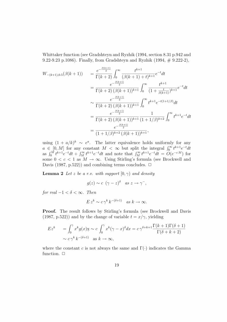
Whittaker function (see Gradshteyn and Ryzhik (1994, section 8.31 p.942 and9.22-9.23 p.1086). Finally, from Gradshteyn and Ryzhik (1994, # 9.222-2),

W!(k+1),0.5()(k + 1)) =e!

!(k+1)2

#(k + 2)

, "

0

tk+1

()(k + 1) + t)k+1e!tdt

=e!

!(k+1)2

#(k + 2) ()(k + 1))k+1

, "

0

tk+1

(1 + t'(k+1))

k+1e!tdt

' e!!(k+1)

2

#(k + 2) ()(k + 1))k+1

, "

0tk+1e!t(1+1/')dt

=e!

!(k+1)2

#(k + 2) ()(k + 1))k+1

1

(1 + 1/))k+2

, "

0tk+1e!tdt

=e!

!(k+1)2

(1 + 1/))k+2 ()(k + 1))k+1,

using (1 + a/k)k ' ea. The latter equivalence holds uniformly for anya ) [0, M ] for any constant M < " but split the integral

0"0 tk+1e!tdt

as0 M0 tk+1e!tdt +

0"M tk+1e!tdt and note that

0"M tk+1e!tdt = O(e!c M) for

some 0 < c < 1 as M $ ". Using Stirling’s formula (see Brockwell andDavis (1987, p.522)) and combining terms concludes. !

Lemma 2 Let z be a r.v. with support [0, ") and density

g(z) ' c (" & z)" as z $ "!,

for real &1 < $ <". Then

E zk ' c "k k!("+1) as k $".

Proof. The result follows by Stirling’s formula (see Brockwell and Davis(1987, p.522)) and by the change of variable t = x/", yielding

Ezk =, !

0xkg(x)x. ' c

, !

0xk(" & x)"dx = c ""+k+1 #(k + 1)#($ + 1)

#($ + k + 2)

' c "k k!("+1) as k $",

where the constant c is not always the same and #(·) indicates the Gammafunction. !

19

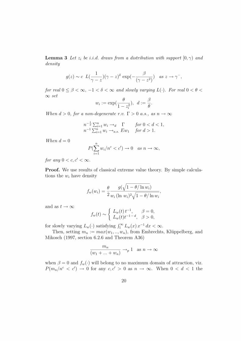
Lemma 3 Let zi be i.i.d. draws from a distribution with support [0, ") anddensity

g(z) ' c L(1

" & z)(" & z)" exp(& )

(" & z2)) as z $ "!,

for real 0 % ) < ", &1 < $ < " and slowly varying L(·). For real 0 < . <" set

wi := exp(.

1& z2i

), d :=)

..

When d > 0, for a non-degenerate r.v. # > 0 a.s., as n$"

n!1d

/ni=1 wi $d # for 0 < d < 1,

n!1 /ni=1 wi $a.s. Ew1 for d > 1.

When d = 0

P (n!

i=1

wi/nc < c#)$ 0 as n$",

for any 0 < c, c# <".

Proof. We use results of classical extreme value theory. By simple calcula-tions the wi have density

fw(wi) =.

2

g(+

1& ./ ln wi)

wi (ln wi)2+

1& ./ ln wi

,

and as t$"fw(t) '

1Lw(t) t!1, ) = 0,Lw(t)t!1! d, ) > 0,

for slowly varying Lw(·) satisfying0"1 Lw(x) x!1 dx <".

Then, setting mn := max(w1, .., wn), from Embrechts, Kluppelberg, andMikosch (1997, section 6.2.6 and Theorem A36)

mn

(w1 + ... + wn)$p 1 as n$"

when ) = 0 and fw(·) will belong to no maximum domain of attraction, viz.P (mn/nc < c#) $ 0 for any c, c# > 0 as n $ ". When 0 < d < 1 the

20

distribution of the wi belongs to the domain of attraction of # and Feller(1966, Theorem IX.8.1) applies. Finally, when d > 1 the wi have boundedfirst moment so by i.i.d.-ness the ergodic theorem applies. !

Proof of Proposition 2.1. Given the i.i.d.ness and bounded variance ofthe xi,t the Lindeberg-Levy CLT applies, as n$". Moreover, for any n bythe martingale di"erence property

covn(1

n12

n!

i=1

xi,t,1

n12

n!

i=1

xi,t+u) = 0 for any u += 0. !

Proof of Proposition 2.2. Ex4t < " when Ef 2

t!1 < ". Evaluating theexpectation of

f 2t = !2 + "2f 2

t!1 + v2t + 2!"ft!1 + 2!vt + 2"ft!1vt,

given Jt!1, yields

E(f 2t | Jt!1) = !2 + ("2 + ()f 2

t!1 + 2!"ft!1 + gt!1.

By Stout (1974, Theorem 3.5.8) the ft are strictly stationary yielding Ef 2t =

Ef 2t!1 when they are finite. Then collect terms and use the law of iterated

expectations. !

Proof of Proposition 3.1. (i) Any instantaneous transformation of a nor-mally distributed r.v. g(Z), where Z is Gaussian, could be expanded in termsof Hermite polynomials when E g(Z)2 < " (see Hannan (1970)). Hence,given

"(

k=0

En e)ki #t!k = e

$2%

2(1!#2i) <" a.s.,

expanding the exp(&ki %t!k/2) yields

Xn,t = ut

"!

mj=0

j=0,1,..

-##

2

./"j=0

mj 12"

j=0 mj!,/"

j=0jmj

"(

j=0

Hmj(%t!j!1), (26)

setting

,k :=1

n

n!

i=1

exp(#2

#

8

1

(1& &2i )

)&ki , k = 0, 1, ...

21

When " = 1, ) > #2# /4 the ,k are finite and the law of iterated logarithm

(LIL) for i.i.d. variates (see Stout (1974, Corollary 5.2.1)) applies yielding

| ,k & ,k |= O

&

' .12k

n12

(ln ln(n .k))12

)

* a.s. for k $", (27)

setting

.k := E exp(#2

#

4

1

(1& &2i )

)&2ki

bounded by assumption for any k ( 0.By the independence of the %t and the orthogonality of the Hermite poly-

nomials

cov

&

'"(

j=0

Hmj(%t!j!1),"(

h=0

Hnh(%t!h!1)

)

* ="(

j=0

$(nj, mj)mj!&"(

j=0

$(nj, 0)$(mj, 0),

where $(·, ·) is the Kronecker delta. Thus,

En(Xn,t &Xt)2 =

"!

mj,nj=0

j=0,1,...

(##

2)/"

j=0(mj+nj) 1

2"j=0 mj!nj!

*

(,/"j=0

jmj& ,/"

j=0jmj

)(,/"j=0

jnj& ,/"

j=0jnj

)*

cov

&

'"(

j=0

Hmj(%t!j!1),"(

j=0

Hnj(%t!j!1)

)

*

= O

&

33'ln ln n

n

"!

mj=0

j=0,1,...

(##

2)2

/"j=0

mj1

2"j=0 mj!

c/"

j=0jmj

)

44*

= O

"ln ln n

nexp(

#2#

4(1& c))

#

,

for some 0 < c = c(b, #2# ) < 1 using Lemma 1.

The nonlinear moving average representation (18) of Xt follows replacing,k with ,k in (26) and re-arranging terms, given the equivalence

"!

m1,...,mq=0m1+...+mq=q

1

m1!...mq!=

"!

n0,...,nq=0n0+...+nq=q1n1+...qnq=q

1

0!n0 ...q!nq

q!

n0!...nq!.

22

We show covariance stationarity of the Xt. By Schwarz inequality

En X2n,t =

1

n2

n!

i=1

En ehi,t!1 +1

n4

n!

i%=j=1

En e0.5(hi,t!1+hj,t!1) (28)

% 1

n2

n!

i=1

En ehi,t!1 +

"1

n

n!

i=1

(En ehi,t!1)12

#2

. (29)

By Lemma 3 En(X2n,t) diverges to infinity in probability at rate n2(

$2%

4!!2) when) < #2

# /4. In fact, the first term on the right hand side of (28) and the secondterm on the right hand side of (29) have the same asymptotic behaviour,

diverging at rate n2($2

%4!!2). This follows considering that given any r.v. Z

with distribution tail regularly varying with index &c (c ( 0) (see Embrechts,Kluppelberg, and Mikosch (1997, Appendix A3.1)) then Z

12 has distribution

tail regularly varying with index &2c. Similarly, En X2n,t converges a.s. to

EX2n,t <" when ) > #2

# /4. Finally, by Lemma 3, En X2n,t $d # as n$" ,

when ) = #2# /4 for a non-degenerate r.v. #. Strict stationarity and ergodicity

follows by using Stout (1974, Theorem 3.5.8) and Royden (1980, Proposition5 and Theorem 3) to (18).(ii) Let us focus for simplicity’s sake on case " = 1. Case " < 1 easily follows.By Schwarz inequality

En X4n,t

=Eu4

t

n4

n!

i=1

En e2 hi,t!1 +Eu4

t

n4

n!

i#=j #=a#=b=1

En e0.5(hi,t!1+hj,t!1+ha,t!1+hb,t!1) (30)

% Eu4t

n4

n!

i=1

En e2 hi,t!1 + Eu4t

"1

n

n!

i=1

(En e2 hi,t!1)14

#4

. (31)

By the same arguments used in part (i) one gets that EnX4n,t converges to

a bounded constant when ) > #2# /2, diverges to infinity in probability at

rate n2(*2% /'!2) when ) < #2

# /2 and converges to a non-degenerate r.v. when) = #2

# /2.Let us deal with the acf. By the cumulants’ theorem (see Leonov and Shiryaev(1959))

covn(X2n,t, X

2n,t+h) =

1

n4

n!

a,b,c,d=1

e$2

%8

/h!1

k=0()k

c +)kd)2

"!

k=0

e$2

%8

/k!1

j=0()j

a+)jb+)j+h

c +)j+hd )2

23

*5e

$2%8 ()k

a+)kb +)k+h

c +)k+hd )2 & e

$2%8 ()k

a+)kb )2e

$2%8 ()k+h

c +)k+hd )2

6

*e$2

%8

/"j=k+1

()ja+)j

b)2

e$2

%8

/"j=k+1

()j+hc +)j+h

d )2 ,

for any integer h > 0, using

cov(m(

i=1

Ci,m(

i=1

Di) =m!

k=1

k!1(

j=1

E(CjDj)cov(Ck, Dk)E(m(

j=k+1

Cj)E(m(

j=k+1

Dj),

which holds for any sequence of independent bivariate r.vs {Ci, Di} withECi Di <". Re-arranging terms yields

covn(X2n,t, X

2n,t+h) =

1

n4

n!

a,b,c,d=1

e$2

%8

/"j=0

[()ja+)j

b)2+()j

c+)jd)2]

*"!

k=0

e$2

%4

/k!1

j=0()j

a+)jb)()

j+hc +)j+h

d )5e

$2%4 ()k

a+)kb )()k+h

c +)k+hd ) & 1

6

% 1

n4

n!

a,b,c,d=1

e$2

%8

/"j=0

()ja+)j

b+)jc+)j

d)2"!

k=0

5e

$2%4 ()k

a+)kb )()k+h

c +)k+hd ) & 1

6.

Note that covn(X2n,t, X

2n,t+h) is non-negative. Expanding the exponential

term in [ · ] brackets

covn(X2n,t, X

2n,t+h) =

"!

k=0

"!

r=1

(#2

#

4)r 1

r!

*&

' 1

n4

n!

a,b,c,d=1

e$2

%8

/"j=0

()ja+)j

b+)jc+)j

d)2 (&ka + &k

b )r (&k+h

c + &k+hd )r

)

* .

Using(a + b + c + d)2 < 4(a2 + b2 + c2 + d2),

which holds for any real a, b, c, d except for case a=b=c=d, when ) > #2# /2,

we can find a 0 < c <" such that

E covn(X2n,t, X

2n,t+h)

= O-, 1

0

, 1

0

, 1

0

, 1

0(&k

a + &kb )

r(&k+hc + &k+h

d )re!c( 1

1!#a+ 1

1!#b+ 1

1!#c+ 1

1!#d)d&ad&bd&cd&d

..

24

Expanding the two binomial terms and using Lemma 1 repeatedly yields, forsome 0 < c < 1,

E covn(X2n,t, X

2n,t+h) = O(

"!

r=1

#2r#

r!

chr

1& c2r) = O(e*2

% ch &1 ) = O(ch) as h$". !

Proof of Proposition 3.2. From generalizations of Minkowski’s inequality(see Hardy, Littlewood, and Polya (1964, Theorems 24 and 25)), for anysequence ai,j (i = 1, . . . , j = 1, . . . , n) one obtains:

&

'"!

i=0

(1

n

n!

j=1

(ai,j)12 )2

)

*

12

% 1

n

n!

j=1

" "!

i=0

ai,j

# 12

%&

'"!

i=0

1

n

n!

j=1

(ai,j)12

)

* , (32)

yielding (22) with

Xn,t := ut

&

'"

1

n

n!

i=1

-+i

1& &i

. 12

#2

+"!

k=0

'2k2e&t!k

)

*

12

,

Xn,t := ut

"1

n

n!

i=1

-+i

1& &i

. 12

+"!

k=0

' k2e

12&t!k

#

,

setting

'k :=1

n

n!

i=1

&ki .

(i) Let us initially focus on Xn,t. Let us focus on case " = 1, ) = 0 forsimplicity’s sake. The other cases easily follows. We show that En |Xn,t &X t |= o(1) as n$". Consider

|Xn,t&X t |%|ut |"77777

1

n

n!

i=1

-+i

1& &i

. 12

& E-

+i

1& &i

. 12

77777 +"!

k=0

| 'k & 'k | e12&t!k

#

.

(33)

When $ > &1/2 then E+12i /(1 & &i)

12 < " by Lippi and Za"aroni (1998,

Lemma 1) and using the LIL for i.i.d. variates one gets for the first term onthe right hand side of (33)

777771

n

n!

i=1

-+

1& &i

. 12

& E-

+

1& &i

. 12

77777 = O

"

(ln ln n

n)

12

#

a.s.

25

For the second term on the right hand side of (33), setting /k := E ek&t forreal k, consider

"!

k=0

| ' k2& ' k

2| e

12&t

= / 12

"!

k=0

| ' k2& ' k

2| +

"!

k=0

| ' k2& ' k

2| (e

12&t & / 1

2). (34)

Let us focus on the first term on the right hand side of (34). By the LIL fori.i.d. variates, for real k

'k & 'k ' 212 var

12 (&k

i )ln ln(n var(&k

i ))

n

12

a.s. for n$". (35)

When ) > 0 by Lemma 1 var12 (&

k2i ) % E

12 (&k

i ) = O(ck) as k $ " for some0 < c < 1 and thus the result easily follows. When ) = 0 then by Lemma 2

var(&ki ) ' E(&2k

i ) ' c k!("+1) as k $" and summability of var12 (&

k2i ) is not

guaranteed anymore. We consider the following truncating argument. Forarbitrary s <"

/ 12

"!

k=0

| ' k2& ' k

2|= / 1

2

s!

k=0

| ' k2& ' k

2| +/ 1

2

"!

k=s+1

| ' k2& ' k

2| .

For the first term above

s!

k=0

| ' k2& ' k

2|= O

"

(ln ln n

n)

12

#

a.s. n$"

by (35) and for the second term

"!

k=s+1

| ' k2& ' k

2|%

"!

k=s+1

' k2

+"!

k=s+1

' k2

(36)

=1

n

n!

i=1

&(s+1)

2i

1& &12i

+"!

k=s+1

' k2

= O

&

3'E&

(s+1)2

i

1& &i+

"!

k=s+1

' k2

)

4* a.s. for n$". (37)

26

By Lippi and Za"aroni (1998, Lemma 1) and Lemma 2 it easily follows thatboth terms on the right hand side of (37) are well defined when $ > 0.Moreover both are O(s!") which can be made arbitrarily small by choosings large enough.

Let us deal with the second term on the right hand side of (34). Notethat {e 1

2&t & / 12} is an i.i.d. sequence with zero mean and finite variance. By

the same truncating argument just used, for arbitrary s,

"!

k=0

| ' k2& ' k

2| (e

&t!k2 & / 1

2)

=s!

k=0

| ' k2& ' k

2| (e

&t!k2 & / 1

2) +

"!

k=s+1

| ' k2& ' k

2| (e

12&t!k & / 1

2).

For the first term above

varn(s!

k=0

| ' k2& ' k

2| (e

12&t!k & / 1

2))

= var(e12&t)

s!

k=0

$' k

2& ' k

2

%2= O

"ln ln n

n

#

a.s. for n$".

For the second term, using var(A&B) % (+

var(A) ++

var(B))2 for any r.vsA, B with finite variance ,

varn("!

k=s+1

| ' k2& ' k

2| (e

12&t!k & / 1

2))

= O

&

3'1

n2

n!

i,j=1

&(s+1)

2i &

(s+1)2

j

1& (&i &j)12

+"!

k=s+1

'2k2

)

4*

= O

&

3'E&

(s+1)2

i &(s+1)

2j

1& (&i &j)12

+"!

k=s+1

'2k2

)

4* a.s. for n$". (38)

Both terms on the left hand side of (38) are well defined when $ > &1/2. Infact

1

n2

n!

i,j=1

&ki &k

j

1& (&i &j)12

% 2

n2

n!

i,j=1

&ki &k

j

1& &i &j%

"1

n

n!

i=1

&ki

(1& &i)12

#2

,

27

since (1 & &i&j)2 ( (1 & &2i )(1 & &2

j ). Boundedness follows by Lippi andZa"aroni (1998, Lemma 1). Secondly,

/"k=s+1 '2

k2

is summable for $ > &1/2

by Lemma 2. Both terms are O(s!2 ") and can be made arbitrarily for s largeenough.

Combining terms, convergence in first mean of Xn,t to X t occurs when$ > 0. Boundedness of the X t follows re-writing

X t = ut

"

E-

+i

1& &i

. 12

+ / 12

"!

k=0

' k2

+"!

k=0

' k2(e

12&t!k & / 1

2)

#

. (39)

Then/"

k=0 ' k2

<" when $ > 0 and | /"k=0 ' k

2(e

12&t!k & / 1

2) |<" a.s. when

$ > &1/2 given independence and finite variance of the {e 12&t & / 1

2} and

/"k=0 '2

k2

< " by Billingsley (1986, Theorem 22.6). Strict stationarity and

ergodicity follows by Stout (1974, Theorem 3.5.8). Finally it easily followsthat covariance stationarity for both levels and squares requires

/"k=0 ' k

2<"

and thus $ > 0.The same results apply for Xn,t when

/"k=1 '2

k < " which requires $ >&1/2.(ii) When " < 1 or " = 1, ) > 0, then 'k = O(ck) as k $ " for some0 < c < 1 and the result easily follows. When " = 1, ) = 0 easy calculationsshow that EX

4t <" requires

/"k=0 'k <" and thus $ > 0. Moreover

cov(X2t , X

2t+h)

' c!

k=0

' k2' (k+h)

2+ c#(

!

k=0

' k2' (k+h)

2)2 + c##

!

k=0

'2k2'2

(k+h)2

as h$",

and by"!

k=0

'2k2'2

(k+h)2

= O(maxk>h/2

'2k2),

the first terms on the right hand side above dominates yielding

cov(X2t , X

2t+h) ' c

"!

k=0

' k2' (k+h)

2' c#'h

2' c## h!("+1) as h$"

by (20) and summability of the 'k. Along the same lines, it follows thatcovariance stationarity of the X2

t requires/"

k=1 '2k2

<" and thus $ > &1/2,

28

yielding

cov(X2t , X

2t+h) ' c

"!

k=1

'2k2'2

(k+h)2

' c#'2h2' c## h!2("+1) as h$".!

Proof of Proposition 3.3. Adapting the arguments developed in part (i)of the proof of Proposition 3.2 above to

En(Xn,t &Xt)2 = #2

#

"!

k=1

('k & 'k)2 ,

part (i) follows. The limit aggregate coincides with the long memory nonlin-ear MA of Robinson and Za"aroni (1998) who establish the memory prop-erties of part (ii), given the asymptotic behaviour of the 'j characterized inLemma 1 and 2. !

References

Andersen, T. (1994): “Stochastic autoregressive volatility: a frameworkfor volatility modelling,” Mathematical Finance, 4/2, 75–102.

Andersen, T., and T. Bollerslev (1997): “Heterogeneous informationarrivals and return volatility dynamics: uncovering the long-run in highfrequency returns,” Journal of Finance, 52, 975–1005.

Baillie, R. T., T. Bollerslev, and H. O. A. Mikkelsen(1996): “Fractionally integrated generalized autoregressive conditionalheteroskedasticity,” Journal of Econometrics, 74/1, 3–30.

Billingsley, P. (1986): Probability and Measure. New York: Wiley, secondedn.

Bollerslev, T. (1986): “Generalized autoregressive conditional het-eroskedasticity,” Journal of Econometrics, 31, 302–327.

Breidt, F., N. Crato, and de Lima P. (1998): “Modelling long-memorystochastic volatility,” Journal of Econometrics, 73, 325–334.

Brockwell, P., and R. Davis (1987): Time series: theory and methods.New York: Springer-Verlag.

29

Comte, F., and E. Renault (1998): “Long memory in continuous-timestochastic volatility models,” Mathematical Finance, 8/4, 291–323.

Ding, Z., and C. Granger (1996): “Modeling volatility persistence ofspeculative returns: a new approach,” Journal of Econometrics, 73, 185–215.

Ding, Z., C. W. J. Granger, and R. F. Engle (1993): “A long memoryproperty of stock market and a new model,” Journal of Empirical Finance,1, 83–106.

Embrechts, P., C. Kluppelberg, and T. Mikosch (1997): Modellingextremal events in insurance and finance. Berlin: Springer.

Esary, J., F. Proschan, and D. Walkup (1967): “Association of ran-dom variables with applications,” Annals of Mathematical Statistics, 38,1466–1474.

Feller, W. (1966): An introduction to probability theory and its applica-tions, vol. II. New York: Wiley.

Ghysels, E., A. Harvey, and E. Renault (1996): “Stochastic Volatil-ity,” in Statistical methods of finance. Handbook of Statistics, ed. byG. Maddala,and C. Rao, vol. 14, pp. 119–191. Amsterdam; New Yorkand Oxford: Elsevier, North Holland.

Giraitis, L., and D. Surgailis (1986): “Multivariate Appell polynomialsand the central limit theorem,” in Dependence in probability and Statistics,ed. by M. Taqqu,and A. Eberlein. Birkhauser.

Gradshteyn, I., and I. Ryzhik (1994): Table of integrals, series andproducts. San Diego: Academic Press, 5 edn.

Granger, C. (1980): “Long memory relationships and the aggregation ofdynamic models,” Journal of Econometrics, 14, 227–238.

Granger, C. W. J., and Z. Ding (1996): “Varieties of long memorymodels,” Journal of Econometrics, 73, 61–77.

Hannan, E. (1970): Multiple time series. New York: Wiley.

30

Hardy, G., J. Littlewood, and G. Polya (1964): Inequalities. Cam-bridge (UK): Cambridge University Press.

Harvey, A. (1998): “Long memory in stochastic volatility,” in Forecastingvolatility in financial markets, ed. by J. Knight,and S. Satchell. London:Butterworth-Heineman, forthcoming.

Leipus, R., and M. Viano (1999): “Aggregation in ARCH models,”Preprint.

Leonov, V., and A. Shiryaev (1959): “On a method of calculation ofsemi-invariants,” Theory of Probability Applications, 4, 319–329.

Lippi, M., and P. Zaffaroni (1998): “Aggregation of simple linear dy-namics: exact asymptotic results,” Econometrics Discussion Paper 350,STICERD-LSE.

Meddahi, N., and E. Renault (1996): “Aggregation and marginalizationof GARCH and Stochastic Volatility models,” Preprint.

Nelson, D. (1991): “Conditional heteroscedasticity in asset pricing: a newapproach,” Econometrica, 59, 347–370.

Nijman, T., and E. Sentana (1996): “Marginalization and contempora-neous aggregation in multivariate GARCH processes,” Journal of Econo-metrics, 71, 71–87.

Robinson, P. M. (1978): “Statistical inference for a random coe!cientautoregressive model,” Scandinavian Journal of Statistics, 5, 163–168.

Robinson, P. M. (1991): “Testing for strong serial correlation and dy-namic conditional heteroskedasticity in multiple regression,” Journal ofEconometrics, 47, 67–84.

Robinson, P. M. (1999): “The memory of stochastic volatility models,”Preprint.

Robinson, P. M., and P. Zaffaroni (1997): “Modelling nonlinearity andlong memory in time series,” in Nonlinear Dynamics and Time Series, ed.by C. Cutler,and D. Kaplan. Providence (NJ): American MathematicalSociety.

31

Robinson, P. M., and P. Zaffaroni (1998): “Nonlinear time series withlong memory: a model for stochastic volatility,” Journal of Statistical Plan-ning and Inference, 68, 359–371.

Royden, H. (1980): Real analysis. London: Macmillan.

Stout, W. (1974): Almost sure convergence. Academic Press.

Tauchen, G., and M. Pitts (1983): “The price variability volume rela-tionship on speculative markets,” Econometrica, 51, 485–505.

Taylor, S. (1986): Modelling Financial Time Series. Chichester (UK): Wi-ley.

Zaffaroni, P. (2000): “Contemporaneous aggregation of GARCH pro-cesses,” Econometrics Discussion Paper 383, STICERD-LSE.

32

!!"#$%&'()*)+#,(,+#%+,(

(

List of other working papers:

2002

1. Paolo Zaffaroni, Gaussian inference on Certain Long-Range Dependent Volatility Models, WP02-12

2. Paolo Zaffaroni, Aggregation and Memory of Models of Changing Volatility, WP02-11 3. Jerry Coakley, Ana-Maria Fuertes and Andrew Wood, Reinterpreting the Real Exchange Rate

- Yield Diffential Nexus, WP02-10 4. Gordon Gemmill and Dylan Thomas , Noise Training, Costly Arbitrage and Asset Prices:

evidence from closed-end funds, WP02-09 5. Gordon Gemmill, Testing Merton's Model for Credit Spreads on Zero-Coupon Bonds, WP02-

08 6. George Christodoulakis and Steve Satchell, On th Evolution of Global Style Factors in the

MSCI Universe of Assets, WP02-07 7. George Christodoulakis, Sharp Style Analysis in the MSCI Sector Portfolios: A Monte Caro

Integration Approach, WP02-06 8. George Christodoulakis, Generating Composite Volatility Forecasts with Random Factor

Betas, WP02-05 9. Claudia Riveiro and Nick Webber, Valuing Path Dependent Options in the Variance-Gamma

Model by Monte Carlo with a Gamma Bridge, WP02-04 10. Christian Pedersen and Soosung Hwang, On Empirical Risk Measurement with Asymmetric

Returns Data, WP02-03 11. Roy Batchelor and Ismail Orgakcioglu, Event-related GARCH: the impact of stock dividends

in Turkey, WP02-02 12. George Albanis and Roy Batchelor, Combining Heterogeneous Classifiers for Stock Selection,

WP02-01

2001

1. Soosung Hwang and Steve Satchell , GARCH Model with Cross-sectional Volatility; GARCHX Models, WP01-16

2. Soosung Hwang and Steve Satchell, Tracking Error: Ex-Ante versus Ex-Post Measures, WP01-15

3. Soosung Hwang and Steve Satchell, The Asset Allocation Decision in a Loss Aversion World, WP01-14

4. Soosung Hwang and Mark Salmon, An Analysis of Performance Measures Using Copulae, WP01-13

5. Soosung Hwang and Mark Salmon, A New Measure of Herding and Empirical Evidence, WP01-12

6. Richard Lewin and Steve Satchell, The Derivation of New Model of Equity Duration, WP01-11

7. Massimiliano Marcellino and Mark Salmon, Robust Decision Theory and the Lucas Critique, WP01-10

8. Jerry Coakley, Ana-Maria Fuertes and Maria-Teresa Perez, Numerical Issues in Threshold Autoregressive Modelling of Time Series, WP01-09

9. Jerry Coakley, Ana-Maria Fuertes and Ron Smith, Small Sample Properties of Panel Time-series Estimators with I(1) Errors, WP01-08

10. Jerry Coakley and Ana-Maria Fuertes, The Felsdtein-Horioka Puzzle is Not as Bad as You Think, WP01-07

11. Jerry Coakley and Ana-Maria Fuertes, Rethinking the Forward Premium Puzzle in a Non-linear Framework, WP01-06

12. George Christodoulakis, Co-Volatility and Correlation Clustering: A Multivariate Correlated ARCH Framework, WP01-05

13. Frank Critchley, Paul Marriott and Mark Salmon, On Preferred Point Geometry in Statistics, WP01-04

14. Eric Bouyé and Nicolas Gaussel and Mark Salmon, Investigating Dynamic Dependence Using Copulae, WP01-03

15. Eric Bouyé, Multivariate Extremes at Work for Portfolio Risk Measurement, WP01-02 16. Erick Bouyé, Vado Durrleman, Ashkan Nikeghbali, Gael Riboulet and Thierry Roncalli,

Copulas: an Open Field for Risk Management, WP01-01

2000

1. Soosung Hwang and Steve Satchell , Valuing Information Using Utility Functions, WP00-06 2. Soosung Hwang, Properties of Cross-sectional Volatility, WP00-05 3. Soosung Hwang and Steve Satchell, Calculating the Miss-specification in Beta from Using a

Proxy for the Market Portfolio, WP00-04 4. Laun Middleton and Stephen Satchell, Deriving the APT when the Number of Factors is

Unknown, WP00-03 5. George A. Christodoulakis and Steve Satchell, Evolving Systems of Financial Returns: Auto-

Regressive Conditional Beta, WP00-02 6. Christian S. Pedersen and Stephen Satchell, Evaluating the Performance of Nearest

Neighbour Algorithms when Forecasting US Industry Returns, WP00-01

1999

1. Yin-Wong Cheung, Menzie Chinn and Ian Marsh, How do UK-Based Foreign Exchange Dealers Think Their Market Operates?, WP99-21

2. Soosung Hwang, John Knight and Stephen Satchell, Forecasting Volatility using LINEX Loss Functions, WP99-20

3. Soosung Hwang and Steve Satchell, Improved Testing for the Efficiency of Asset Pricing Theories in Linear Factor Models, WP99-19

4. Soosung Hwang and Stephen Satchell, The Disappearance of Style in the US Equity Market, WP99-18

5. Soosung Hwang and Stephen Satchell, Modelling Emerging Market Risk Premia Using Higher Moments, WP99-17

6. Soosung Hwang and Stephen Satchell, Market Risk and the Concept of Fundamental Volatility: Measuring Volatility Across Asset and Derivative Markets and Testing for the Impact of Derivatives Markets on Financial Markets, WP99-16

7. Soosung Hwang, The Effects of Systematic Sampling and Temporal Aggregation on Discrete Time Long Memory Processes and their Finite Sample Properties, WP99-15

8. Ronald MacDonald and Ian Marsh, Currency Spillovers and Tri-Polarity: a Simultaneous Model of the US Dollar, German Mark and Japanese Yen, WP99-14

9. Robert Hillman, Forecasting Inflation with a Non-linear Output Gap Model, WP99-13 10. Robert Hillman and Mark Salmon , From Market Micro-structure to Macro Fundamentals: is

there Predictability in the Dollar-Deutsche Mark Exchange Rate?, WP99-12 11. Renzo Avesani, Giampiero Gallo and Mark Salmon, On the Evolution of Credibility and

Flexible Exchange Rate Target Zones, WP99-11 12. Paul Marriott and Mark Salmon, An Introduction to Differential Geometry in Econometrics,

WP99-10 13. Mark Dixon, Anthony Ledford and Paul Marriott, Finite Sample Inference for Extreme Value

Distributions, WP99-09 14. Ian Marsh and David Power, A Panel-Based Investigation into the Relationship Between

Stock Prices and Dividends, WP99-08 15. Ian Marsh, An Analysis of the Performance of European Foreign Exchange Forecasters,

WP99-07 16. Frank Critchley, Paul Marriott and Mark Salmon, An Elementary Account of Amari's Expected

Geometry, WP99-06 17. Demos Tambakis and Anne-Sophie Van Royen, Bootstrap Predictability of Daily Exchange

Rates in ARMA Models, WP99-05 18. Christopher Neely and Paul Weller, Technical Analysis and Central Bank Intervention, WP99-

04 19. Christopher Neely and Paul Weller, Predictability in International Asset Returns: A Re-

examination, WP99-03

20. Christopher Neely and Paul Weller, Intraday Technical Trading in the Foreign Exchange Market, WP99-02

21. Anthony Hall, Soosung Hwang and Stephen Satchell, Using Bayesian Variable Selection Methods to Choose Style Factors in Global Stock Return Models, WP99-01

1998

1. Soosung Hwang and Stephen Satchell, Implied Volatility Forecasting: A Compaison of Different Procedures Including Fractionally Integrated Models with Applications to UK Equity Options, WP98-05

2. Roy Batchelor and David Peel, Rationality Testing under Asymmetric Loss, WP98-04 3. Roy Batchelor, Forecasting T-Bill Yields: Accuracy versus Profitability, WP98-03 4. Adam Kurpiel and Thierry Roncalli , Option Hedging with Stochastic Volatility, WP98-02 5. Adam Kurpiel and Thierry Roncalli, Hopscotch Methods for Two State Financial Models,

WP98-01